Application of Minimal Cut Sets Algorithm to theOptimization of Plasmid and Recombinant Protein

Production

Tiago Filipe dos Santos Roseiro

Thesis to obtain the Master of Science Degree in

Biological Engineering

Supervisor(s)

Prof. Isabel Cristina de Almeida Pereira da RochaProf. Duarte Miguel De França Teixeira dos Prazeres

Examination CommitteeChairperson: Prof. Gabriel António Amaro Monteiro

Supervisor: Prof. Isabel Cristina de Almeida Pereira da RochaMember of the Committee: Dr. Sara Alexandra Gomes Correia

November 2018

Acknowledgments/Agradecimentos

First and foremost, I would like to thank my thesis supervisors Prof. Miguel Prazeres andProf. Isabel Rocha for the time spent and valuable guidance and support. Their advice wasextremely important throughout this project.

I want to take this opportunity to express my gratitude to Prof. Miguel Rocha and hiswhole lab for welcoming in their work and facilities during my stay in Braga. I want to give aspecial note to Vitor Vieira, for being extremely supportive and taking the time to teach methroughout this process. This research project would not have been finished successfully withouthis continuous support and readily available assistance (even when I was back in Lisbon). Onanother special note, I would like to thank Ana Sofia Ferreira for her last minute, but extremelyvaluable and crucial help, in this thesis. Without her, this project would not have the samequality.

I would like to gratefully acknowledge to all my friends that have been part of this 5-yearjourney. To my friends and colleagues Adriana and Catia, I could not ask for better peopleto spend these 5 years working and laughing together. I wish you the best in your next newjourneys. This one was truly amazing. To my Biodanish friends (Cat, Danylo, Goncalo, Ines,Joana, Susana e Tomas) it was amazing and a pleasure to meet you all and, I hope we all meetagain in a near future. I would like to give a special word to David and Cat, for their amazingsupport throughout this work. You guys were always there for me and I can not thank youenough for that.

Finalmente, gostaria de agradecer a minha familia, por tudo o que abdicaram e fizeram pormim para ser a pessoa que sou hoje. Obrigado a todos!

i

ii

Abstract

Recombinant proteins (e.g. biopharmaceuticals, food processing enzymes, etc) are increas-ingly becoming more relevant in Biotechnology and Pharmaceutical industries. Current ap-proaches for microbial strain optimization for industrial purposes rely heavily on modern SystemsBiology. Regarding in silico methods, the most prominent currently comprise constraint-basedmodelling of cell metabolism, from central carbon metabolism to genome-scale models. Suchapproaches are used to solve metabolic engineering problems to fulfill an industrial objectiveand can be divided into phenotype prediction and pathway analysis (PA) methods. Unlike phe-notype prediction, PA methods try to provide a more unbiased perspective but heavily dependon the complexity and scale of the model.

The aim of this work is to apply a PA method (minimal cut sets) to the optimization ofplasmid and recombinant protein production. For this purpose, a novel implementation of anefficient algorithm for enumeration of minimal cut sets developed by Vieira (2015) was used.

The case study selected is based on a work performed by Pandey et al. (2018) and it involvesinterferon gamma production. Using an E. coli central metabolism model and a genome-scalemodel, different MCS enumeration problems were developed, for which knockout strategies weredetermined. An exploratory data analysis (principal component analysis and hierarchical clus-tering analysis) of the solutions was performed to select a few knockout sets for further analysis.The latter was performed to study the flux distributions and highlight different mechanismsof plasmid and/or product synthesis. From these analysis, it was possible to conclude thatdeletion of genes pgi, pck and udhA/ptnAB seem promising to increase in vivo plasmid and/orrecombinant protein production. In addition, a further detailed analysis regarding genome-scalemodelling would be beneficial to corroborate the results and add new knockout suggestions.

Keywords: Recombinant proteins; Constraint-based metabolic modelling; Flux balanceanalysis; Metabolic engineering; Pathway analysis; Minimal cut sets

iii

iv

Resumo

As proteınas recombinantes sao cada vez mais relevantes nas industrias biotecnologicas efarmaceuticas no que diz respeito, por exemplo, a agentes terapeuticos e a producao de enzimasimportantes ao processamento alimentar.

As abordagens atuais para a otimizacao de estripes microbianas para fins industriais recorremextensamente ao pensamento moderno da biologia de sistemas. Relativamente aos metodos insilico, estes usam, entre outros, modelos matematicos baseados em restricoes do metabolismocelular, desde metabolismo central a modelos de escala genomica. Tais abordagens sao usadaspara resolver problemas de engenharia metabolica para cumprir um objetivo industrial e podemser divididas em metodos de previsao de fenotipos e de analise de vias metabolicas (AVM). Aocontrario da previsao de fenotipos, os metodos de AVM tentam fornecer uma perspetiva maisimparcial, mas sao dependentes da complexidade e da escala dos modelos metabolicos.

Com este trabalho, o objetivo e aplicar um metodo AVM (minimal cut sets - MCS) naotimizacao da producao de plasmıdeos e proteınas recombinantes. Para tal, utilizou-se uma novaimplementacao de um algoritmo eficiente para a enumeracao de minimal cut sets, desenvolvidapor Vieira (2015), num caso de estudo.

Este caso de estudo e baseado num trabalho realizado por Pandey et al. (2018) e envolvea producao de interferao gama. Usando um modelo de metabolismo central e um modelo aescala genomica de E. coli, foram desenvolvidos diferentes problemas de enumeracao de MCS,para os quais foram determinadas estrategias de delecao. Uma analise exploratoria de dados(analise de componentes principais e analise de clusters de metodos hierarquicos) das solucoes foirealizada para selecionar alguns conjuntos de delecoes para posterior analise. Esta ultima analisefoi realizada com o intuito de estudar as distribuicoes de fluxo e destacar diferentes padroes emecanismos de sıntese de plasmıdeos e/ou produtos.

A partir destas analises, foi possıvel concluir que delecao dos genes pgi, pck e udhA/ptnAB po-dem ser uma aposta promissora para aumentar a producao in vivo de plasmıdeos e/ou proteınasrecombinantes. Adicionalmente, uma analise mais detalhada utilizando modelos a escala genom-ica seria benefica para corroborar os resultados encontrados e sugerir novos knockouts.

Palavras-Chave: Proteinas recombinantes; Modelacao metabolica com base em re-stricoes; Flux balance analysis; Engenharia metabolica; Analise de vias metabolicas; Minimalcut sets

v

vi

Contents

List of Figures ix

List of Tables xi

List of Acronyms xiii

1 Introduction 11.1 Recombinant Proteins . . . . . . . . . . . . . . . . . . . . . . . . . . . . . . . . . 11.2 Systems Biology . . . . . . . . . . . . . . . . . . . . . . . . . . . . . . . . . . . . 21.3 Metabolic Networks . . . . . . . . . . . . . . . . . . . . . . . . . . . . . . . . . . 3

1.3.1 Stoichiometric Matrix . . . . . . . . . . . . . . . . . . . . . . . . . . . . . 51.3.2 Genome-scale Metabolic Models . . . . . . . . . . . . . . . . . . . . . . . 61.3.3 Mathematical Modelling Approaches . . . . . . . . . . . . . . . . . . . . . 7

1.4 Phenotype Prediction . . . . . . . . . . . . . . . . . . . . . . . . . . . . . . . . . 111.4.1 Flux Balance Analysis . . . . . . . . . . . . . . . . . . . . . . . . . . . . . 111.4.2 Flux Variability Analysis . . . . . . . . . . . . . . . . . . . . . . . . . . . 121.4.3 Parsimonious Enzyme Usage FBA . . . . . . . . . . . . . . . . . . . . . . 13

1.5 Pathway Analysis . . . . . . . . . . . . . . . . . . . . . . . . . . . . . . . . . . . . 131.5.1 Nullspace Analysis . . . . . . . . . . . . . . . . . . . . . . . . . . . . . . . 131.5.2 Convex Analysis . . . . . . . . . . . . . . . . . . . . . . . . . . . . . . . . 141.5.3 Elementary Flux Modes . . . . . . . . . . . . . . . . . . . . . . . . . . . . 151.5.4 Minimal Cut Sets . . . . . . . . . . . . . . . . . . . . . . . . . . . . . . . . 16

1.6 Motivation and Objectives . . . . . . . . . . . . . . . . . . . . . . . . . . . . . . . 18

2 Materials and Methods 212.1 Metabolic Models . . . . . . . . . . . . . . . . . . . . . . . . . . . . . . . . . . . . 21

2.1.1 Central Metabolism Model . . . . . . . . . . . . . . . . . . . . . . . . . . 212.1.2 Genome-scale Model . . . . . . . . . . . . . . . . . . . . . . . . . . . . . . 222.1.3 Model Formulations . . . . . . . . . . . . . . . . . . . . . . . . . . . . . . 22

2.2 Cellular Constraints . . . . . . . . . . . . . . . . . . . . . . . . . . . . . . . . . . 262.3 Enumeration Algorithm . . . . . . . . . . . . . . . . . . . . . . . . . . . . . . . . 262.4 Statistical Methods . . . . . . . . . . . . . . . . . . . . . . . . . . . . . . . . . . . 28

2.4.1 Principal Component Analysis . . . . . . . . . . . . . . . . . . . . . . . . 282.4.2 Cluster Analysis . . . . . . . . . . . . . . . . . . . . . . . . . . . . . . . . 28

2.5 Tools and Software . . . . . . . . . . . . . . . . . . . . . . . . . . . . . . . . . . . 302.5.1 The R Programming Language . . . . . . . . . . . . . . . . . . . . . . . . 30

vii

2.5.2 MATLAB . . . . . . . . . . . . . . . . . . . . . . . . . . . . . . . . . . . . 312.5.3 The Java Programming Language . . . . . . . . . . . . . . . . . . . . . . 31

3 Results and Discussion 333.1 Central Metabolism Model . . . . . . . . . . . . . . . . . . . . . . . . . . . . . . 33

3.1.1 Data Processing . . . . . . . . . . . . . . . . . . . . . . . . . . . . . . . . 333.1.2 Exploratory Data Analysis . . . . . . . . . . . . . . . . . . . . . . . . . . 343.1.3 Detailed Network Analysis . . . . . . . . . . . . . . . . . . . . . . . . . . 49

3.2 Genome-scale Model . . . . . . . . . . . . . . . . . . . . . . . . . . . . . . . . . . 603.2.1 Data Processing . . . . . . . . . . . . . . . . . . . . . . . . . . . . . . . . 613.2.2 Exploratory Data Analysis . . . . . . . . . . . . . . . . . . . . . . . . . . 61

4 Conclusions 694.1 Future Work . . . . . . . . . . . . . . . . . . . . . . . . . . . . . . . . . . . . . . 70

Bibliography 71

A Central Metabolism Model Reaction and Metabolite Lists 79

B Biomolecules Composition 86

C Hierarchical Clustering Analysis 88

viii

List of Figures

1.1 Systems biology research cycle . . . . . . . . . . . . . . . . . . . . . . . . . . . . 31.2 Typical bioreaction network of E.coli central carbon metabolism. . . . . . . . . . 41.3 Toy example of a simplified metabolic network of a microorganism. . . . . . . . . 51.4 Six fields and number of studies for E. coli metabolic GSMs until 2013. . . . . . 71.5 Cellular networks mathematical modelling approaches. . . . . . . . . . . . . . . . 81.6 Mathematical modelling: scope and interactions. . . . . . . . . . . . . . . . . . . 81.7 Principles of the stoichiometric modeling framework. . . . . . . . . . . . . . . . . 111.8 The conceptual basis of a FBA problem. . . . . . . . . . . . . . . . . . . . . . . . 121.9 Representation of a pointed convex polyhedral cone for a metabolic network. . . 141.10 Simple example of a biochemical network and its elementary flux modes. . . . . . 161.11 Biochemical network for MCS example. . . . . . . . . . . . . . . . . . . . . . . . 171.12 Elementary modes and minimal cut sets . . . . . . . . . . . . . . . . . . . . . . . 17

2.1 Generic pipeline for enumerating MCSs. . . . . . . . . . . . . . . . . . . . . . . . 272.2 Representation of the agglomerative and the divisive HCA approach. . . . . . . . 30

3.1 Model CMM A Exploratory data analysis results . . . . . . . . . . . . . . . . . . 363.2 Model CMM B Exploratory data analysis results. . . . . . . . . . . . . . . . . . . 393.3 Model CMM C Exploratory data analysis results. . . . . . . . . . . . . . . . . . . 443.4 Model CMM D Exploratory data analysis results. . . . . . . . . . . . . . . . . . . 483.5 MCS1 metabolic flux distribution within central carbon metabolism of E. coli. . 513.6 MCS2 metabolic flux distribution within central carbon metabolism of E. coli. . 543.7 MCS3 metabolic flux distribution within central carbon metabolism of E. coli. . 583.8 Model GSM B Exploratory data analysis. . . . . . . . . . . . . . . . . . . . . . . 623.9 Model GSM C Exploratory data analysis results. . . . . . . . . . . . . . . . . . . 65

C.1 Model CMM A HCA full dendrogram. . . . . . . . . . . . . . . . . . . . . . . . . 89C.2 Model CMM B HCA full dendrogram. . . . . . . . . . . . . . . . . . . . . . . . . 90C.3 Model CMM C HCA full dendrogram. . . . . . . . . . . . . . . . . . . . . . . . . 91C.4 Model GSM B HCA full dendrogram. . . . . . . . . . . . . . . . . . . . . . . . . 92C.5 Model GSM C HCA full dendrogram. . . . . . . . . . . . . . . . . . . . . . . . . 93

ix

x

List of Tables

1.1 Examples of some therapeutically relevant proteins produced by recombinantDNA technology. . . . . . . . . . . . . . . . . . . . . . . . . . . . . . . . . . . . . 1

1.2 Evolution of GSMs of E. coli regarding date and version of model release. . . . . 6

2.1 Model configuration key and main aspects summary . . . . . . . . . . . . . . . . 242.2 Problem configuration key and main aspects summary . . . . . . . . . . . . . . . 252.3 Cellular constraints applied to all the simulations and models used throughout

this work. . . . . . . . . . . . . . . . . . . . . . . . . . . . . . . . . . . . . . . . . 26

3.1 Biologically relevant reactions that were filtered in the CMM data processing step. 343.2 Model CMM A Summary of the suggested knockouts. . . . . . . . . . . . . . . . 353.3 Model CMM A top ten most targeted reactions for knockouts in the overall so-

lutions set (#KO). . . . . . . . . . . . . . . . . . . . . . . . . . . . . . . . . . . . 383.4 Model CMM B Summary of the suggested knockouts. . . . . . . . . . . . . . . . 403.5 Model CMM B top ten most targeted reactions for knockouts in the overall solu-

tions set (#KO). . . . . . . . . . . . . . . . . . . . . . . . . . . . . . . . . . . . . 423.6 Model CMM C Summary of the suggested knockouts. . . . . . . . . . . . . . . . 433.7 Model CMM C top ten most targeted reactions for knockouts in the overall solu-

tions set (#KO). . . . . . . . . . . . . . . . . . . . . . . . . . . . . . . . . . . . . 463.8 Model CMM D Summary of the suggested knockouts. . . . . . . . . . . . . . . . 473.9 Model CMM D top most targeted reactions for knockouts in the overall solutions

set (#KO). . . . . . . . . . . . . . . . . . . . . . . . . . . . . . . . . . . . . . . . 493.10 Model GSM B Summary of the total number of solutions gathered. . . . . . . . . 623.11 Model GSM B top ten most targeted reactions for knockouts in the overall solu-

tions set (#KO). . . . . . . . . . . . . . . . . . . . . . . . . . . . . . . . . . . . . 643.12 Model GSM C Summary of the total number of solutions gathered. . . . . . . . . 653.13 Model GSM C top ten most targeted reactions for knockouts in the overall solu-

tions set (#KO). . . . . . . . . . . . . . . . . . . . . . . . . . . . . . . . . . . . . 67

A.1 List of reactions and respective abbreviations used in the central metabolismmodel network. . . . . . . . . . . . . . . . . . . . . . . . . . . . . . . . . . . . . . 79

A.2 List of metabolites and respective abbreviations used in the central metabolismmodel network. . . . . . . . . . . . . . . . . . . . . . . . . . . . . . . . . . . . . . 83

B.1 Nucleotide composition of pET28a(+) sequence. . . . . . . . . . . . . . . . . . . 86

xi

B.2 Amino acid composition of human interferon gamma fused to an hexa-histidineaffinity tag. . . . . . . . . . . . . . . . . . . . . . . . . . . . . . . . . . . . . . . . 87

B.3 Amino acid composition of plasmid resistance marker phosphotransferase. . . . . 88

xii

List of Acronyms

ATPM Maintenance ATP

BPCY Biomass-product Coupled Yield

CBM Constraint-based Modelling

cMCS Constrained Minimal Cut Set

CMM Central Metabolism Model

COBRA Constraint-based Reconstruction and Analysis

DNA Deoxyribonucleic Acid

dNTP Deoxyribonucleotide Triphosphate

ED Entner-Doudoroff

EFM Elementary Flux Mode

ES Enzyme Subset

FBA Flux Balance Analysis

FVA Flux Variability Analysis

GSM Genome-scale Model

GUI Graphical User Interface

HCA Hierchichal Clustering Analysis

IDE Integrated Development Environment

IFG1 Insulin-like Growth Factor 1

IFNγ Interferon (gamma)

LP Linear Programming

MCS Minimal Cut Set

MFA Metabolic Flux Analysis

xiii

MW Molecular Weight

NGS Next-generation Sequencing

PA Pathway Analysis

PC Principal Component

PCA Principal Component Analysis

pFBA Parsimonious Enzyme Usage FBA

PPP Pentose Phosphate Pathway

PTS Phosphotransferase System

SBML Systems Biology Markup Language

TCA Tricarboxylic Acid

WT Wild-type

xiv

Chapter 1

Introduction

In this Chapter, some biological and computational background knowledge and general def-initions regarding the topics addressed in this thesis are presented.

1.1 Recombinant Proteins

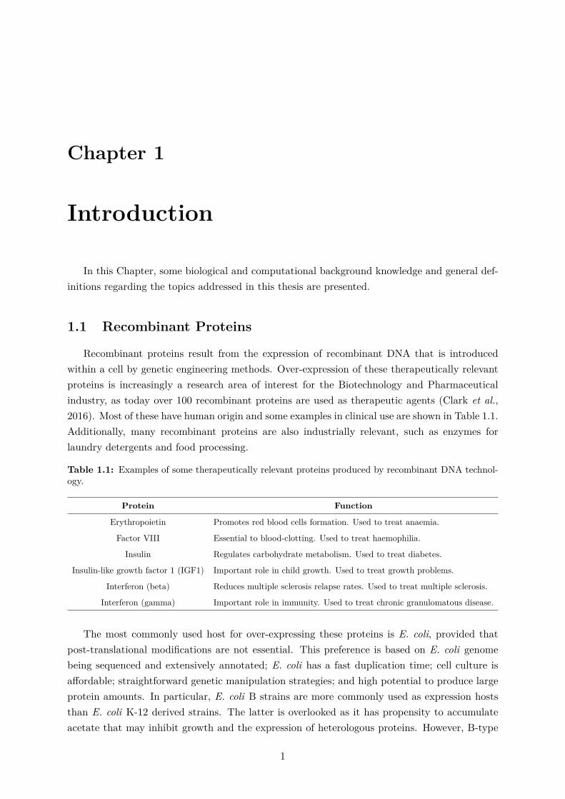
Recombinant proteins result from the expression of recombinant DNA that is introducedwithin a cell by genetic engineering methods. Over-expression of these therapeutically relevantproteins is increasingly a research area of interest for the Biotechnology and Pharmaceuticalindustry, as today over 100 recombinant proteins are used as therapeutic agents (Clark et al.,2016). Most of these have human origin and some examples in clinical use are shown in Table 1.1.Additionally, many recombinant proteins are also industrially relevant, such as enzymes forlaundry detergents and food processing.

Table 1.1: Examples of some therapeutically relevant proteins produced by recombinant DNA technol-ogy.

Protein Function

Erythropoietin Promotes red blood cells formation. Used to treat anaemia.

Factor VIII Essential to blood-clotting. Used to treat haemophilia.

Insulin Regulates carbohydrate metabolism. Used to treat diabetes.

Insulin-like growth factor 1 (IGF1) Important role in child growth. Used to treat growth problems.

Interferon (beta) Reduces multiple sclerosis relapse rates. Used to treat multiple sclerosis.

Interferon (gamma) Important role in immunity. Used to treat chronic granulomatous disease.

The most commonly used host for over-expressing these proteins is E. coli, provided thatpost-translational modifications are not essential. This preference is based on E. coli genomebeing sequenced and extensively annotated; E. coli has a fast duplication time; cell culture isaffordable; straightforward genetic manipulation strategies; and high potential to produce largeprotein amounts. In particular, E. coli B strains are more commonly used as expression hoststhan E. coli K-12 derived strains. The latter is overlooked as it has propensity to accumulateacetate that may inhibit growth and the expression of heterologous proteins. However, B-type

1

strains have shown, for example, plasmid loss that completely arrests protein production and, asa result, non-B strains have gathered a lot of interest in recent years (Liu et al., 2005; Waegemanet al., 2015).

In addition to host-related problems, expressing these recombinant proteins at large-scale hasits own obstacles such as, a high copy number of plasmids may lead to an increased metabolicburden, reducing host growth and often increasing plasmid instability (Liu et al., 2015).

To improve the performance and yield of an expression host one can either manipulate itsgrowth environment or alter its genetic architecture (using mutations and/or gene regulations).These changes may show effects on metabolic network flexibility, flux reaction efficiency andtranscriptional regulation towards a desired product. One of the most common approachestested by researchers to enhance and create an optimized microbial cell factory is to delete oradd genes (Liu et al., 2015; Pandey et al., 2018).

With classical strain optimization methods, new microbial factories were developed based onthe generation of mutants and selection of strains that have desirable phenotypic characteris-tics. These mutants were created by inducing random mutations through chemicals, radiation ortransposons. Then, in a screening test, these mutants would grow in desired conditions and thosethat survived would be further optimized in new conditions or used for the purpose. However,in the start of the 21st century, with the development of systems biology and synthetic biologytowards utilizing cellular network models combined with mathematical methods, metabolic engi-neering rationale had shifted. New computational methods, such as flux balance analysis (FBA)and constraint-based modelling (CBM), emerged and gave birth to a metabolic engineering erawhere strain optimization is first performed in silico and then tested in vivo. Instead of randomlyscreening numerous mutants, computational metabolic engineering is becoming increasingly amore direct and straightforward approach, that is continuously being improved throughout theyears by the addition of new levels of complexity to the networks, as well as development of newmethods and algorithms (Yang et al., 2007).

1.2 Systems Biology

Systems biology is an interdisciplinary field that studies biological systems by describing theinteractions within a system, instead of explaining individual mechanisms (Kirschner, 2005). In amore traditional perspective, biological studies follow a reductionist approach in which individualcomponents of a living system are studied separately. This partitioning method requires a greatworkload amount of analysis and integration - specially with new generation technologies thatpresent high throughputs - that could only be accomplished by innovative computational tools.Consequently, in the 21st century, there has been a shift towards an holistic and integrativemethodology that has evolved not only from the reductionistic problem of dealing with burstinginformations harnessed by high-throughput technologies, but also from lines of work that aimto study functional states of multiple components interactions simultaneously(Palsson, 2000;Westerhoff & Palsson, 2004).

Systems biologists utilize mathematical modelling methods to analyze biological interac-tions represented in different types of networks such as metabolic, transcriptional regulation

2

and signal transduction pathways to understand biological behaviour as a whole rather thancompartmentalized. This field is becoming increasingly significant together with the improve-ment and development of high-throughput technologies and its objective is to enable the studyof biological systems using the maximum amount of information possible at different levels ofcell processes (Widlak, 2013). From cellular activities and metabolism to diagnosis and treat-ment of diseases, these are just some possible applications that can benefit from such approach(Raman & Chandra, 2009). In addition, other biotechnological fields such as genetic therapiesand metabolic engineering can benefit immensely from systematic researches such as the onepresented in this thesis. A schematic systems biology research cycle comprising main steps isdepicted in Figure 1.1.

Figure 1.1: Systems biology research cycle. A new hypothesis is formulated and undergoes experimentaldesign. From the lab experiments new data is generated and a model is constructed. From the latter thehypothesis is evaluated and reformulated and the process restarts until the model explains the data atmaximum extent. From these cycles, new software and technologies may be developed. (From Instituteof Systems Biology, 2018)

1.3 Metabolic Networks

Metabolic networks combine different levels of information in biological systems and describerelationships between metabolites and enzymes in a set of biochemical reactions (Castrillo et al.,2013). Each reaction has key properties that are characterized as follows (Szallasi et al., 2010):

• Stoichiometry: Specifies the molar ratios in which compounds participating in a reactionare consumed or produced. By convention, the stoichiometric coefficient of a compound ispositive if it is produced when the reaction proceeds in its forward direction, and negativeotherwise.

3

• Reversibility: In theory, all reactions are thermodynamically reversible. However, somecan be considered irreversible due to their nearly unidirectionality. This information canbe helpful in constructing accurate metabolic networks.

• Enzymes: Most biochemical reactions are characterized by the participation of an enzymethat facilitates or enables a reaction to proceed. Defining these enzymes allows correlatingbetween network properties and features of the genome encoding those enzymes.

• Kinetics: Describes the dynamics based on the reaction mechanism and enzyme prop-erties. These are defined by rate laws, which are mathematical expressions that describereaction rates as a function of metabolite concentration and specific enzymatic kineticparameters.

A metabolic network can be depicted as a graph where proteins/enzymes, that are edges ofthe network, interact with metabolites (nodes). An example of a metabolic network for centralcarbon flow in E. coli is given in Figure 1.2.

Figure 1.2: Typical bioreaction network of E.coli central carbon metabolism. Arrows indicate theassumed reaction reversibility. Fluxes to biomass building blocks are indicated by solid arrows (FromEmmerling et al., 2002).

The edges usually report an irreversible flux characterized by a uni-directional arrow (v2 inFigure 1.2). Reversible reactions constitute two fluxes in opposite directions and are representedby a bi-directional arrow (v1 in Figure 1.2). Intracellular reactions are edges that connect twogroups of nodes (reactants and products), whereas exchange reactions only need one node withthe edge connecting with the extracellular environment (Chalancon et al., 2013).

4

Overall, metabolic networks play a critical role in numerous studies as this approach canprovide the underlying reactions controlling all the physicochemical states of a cell in largescales.

1.3.1 Stoichiometric Matrix

The stoichiometric matrix, S, is essential to the mathematical representation of metabolicnetworks. It represents each metabolite as a row and each reaction as a column, where thenumerical elements correspond to stoichiometric coefficients. This means that an (i, j) elementrepresents the stoichiometric coefficients of metabolite i taking part in reaction j (Resendis-Antonio, 2013). Each entry depends on the role of metabolites in the reaction as follows:

Sij =

a, number of molecules of i produced in reaction j

−a, number of molecules of i consumed in reaction j

0, if metabolite i does not take part in reaction j

Given a set of reactions, this matrix is constructed in a straightforward manner. As anexample, Figure 1.3 shows the S matrix for a toy example with 10 metabolites and 8 reactions.

Figure 1.3: Toy example of a simplified metabolic network of a microorganism. The microorganismtakes up metabolite A and produces Biomass, products D and E. On the right side, the correspond-ing stoichiometric matrix S, with rows corresponding to metabolites and columns to reactions (FromHanemaaijer et al., 2015).

From this example, exchange reactions with the environment can be represented with internalmetabolites that belong to the metabolic network (A, B, C, D, E, ATP, Biomass) and externalmetabolites that are considered pools or sources of internal metabolites (A out, D out, E out).

If the same compound exists in multiple cellular compartments (for instance, ATP beingpresent in cytosol and mitochondria in eukaryotes), it must be treated as a different metabolitefor each compartment, meaning it must be given a separate row in the matrix (Becker et al.,2007).

5

1.3.2 Genome-scale Metabolic Models

Metabolic models studies were initially restricted to small networks that only representedthe central cell metabolism. One of the earliest studies to systematically analyze E. coli utilizeda simplified constraint based model of acetate overflow (Majewski & Domach, 1990). Subse-quent pre-genome-scale studies scaled-up to include reactions involved in central carbohydratemetabolism, amino acid and nucleotide synthesis to evaluate the biocatalyst production poten-tial. As high-throughput sequencing methods became readily available, aligned with annotatedcontent of E. coli in databases and detailed biochemical reviews, the information added tometabolic networks increased significantly (Baumler et al., 2011). This expansion led to incor-poration into a single systemic model of novel subsystems such as fatty acid synthesis, alternatecarbon metabolism or cell wall synthesis, improving and promoting the metabolic reconstruc-tions to the genome scale, ultimately leading to the reconstruction of genome-scale metabolicmodels (GSMs).

Genome-scale metabolic models have been reconstructed for over 150 organisms so far, in-cluding E. coli (Feist et al., 2009). These reconstructions allow useful predictive calculationsto be performed with high detail. GSMs of E. coli have existed for nearly twenty years as thefirst was released in 2000 by Palsson & Edwards, and this model continues to be expanded andupdated today (McCloskey et al., 2013). It accounts for the products of 660 metabolic genes,and has 627 reactions and 438 metabolites. It includes a biomass reaction based on the measuredcomponents of E. coli biomass that can be used to simulate growth (Edwards & Palsson, 2000).Table 1.2 highlights key events in the evolution of GSMs of E. coli.

Table 1.2: Evolution of GSMs of E. coli regarding date and version of model release. In addition, thenumber of model genes, metabolites and reactions is reported.

Date Version Model Genes Metabolites Reactions Reference

11/05/2000 iJ660 660 438 627 Edwards & Palsson

04/09/2003 iJR904 904 625 931 Reed et al.

28/06/2007 iAF1260 1260 1039 2077 Feist et al.

07/01/2011 iCA1273 1273 1111 2477 Archer et al.

13/10/2011 iJO1366 1366 1136 2251 Orth et al.

GSMs can be applied to study, for instance, evolutionary processes, interspecies interactionsand metabolic engineering problems (McCloskey et al., 2013). Amidst these, metabolic engi-neering problems are some of the most studied using genome-scale models. This field tries todesign new cells by using mathematical and experimental tools in metabolic analysis and mod-ification. Thus, a systematic modelling can help shed some light into the complex nature ofcellular metabolism and improve traditional methods for genetic engineering (e.g. random mu-tagenesis and screening for better phenotypes) by predicting cellular phenotypes from a systemslevel before in vivo implementation (Zhang & Hua, 2016; Yilmaz & Walhout, 2017). Figure 1.4illustrates six fields and number of studies using E. coli metabolic GSMs until 2013. Since then,these numbers have seen an increase.

6

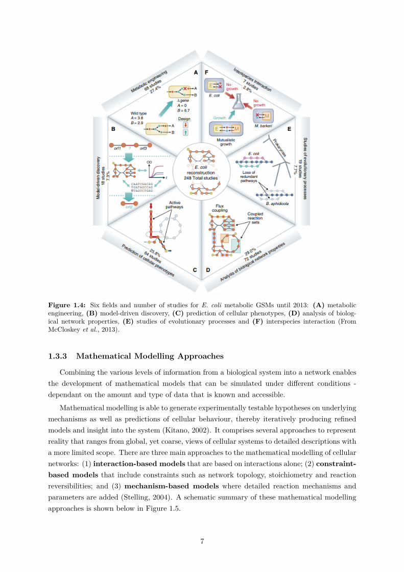
Figure 1.4: Six fields and number of studies for E. coli metabolic GSMs until 2013: (A) metabolicengineering, (B) model-driven discovery, (C) prediction of cellular phenotypes, (D) analysis of biolog-ical network properties, (E) studies of evolutionary processes and (F) interspecies interaction (FromMcCloskey et al., 2013).

1.3.3 Mathematical Modelling Approaches

Combining the various levels of information from a biological system into a network enablesthe development of mathematical models that can be simulated under different conditions -dependant on the amount and type of data that is known and accessible.

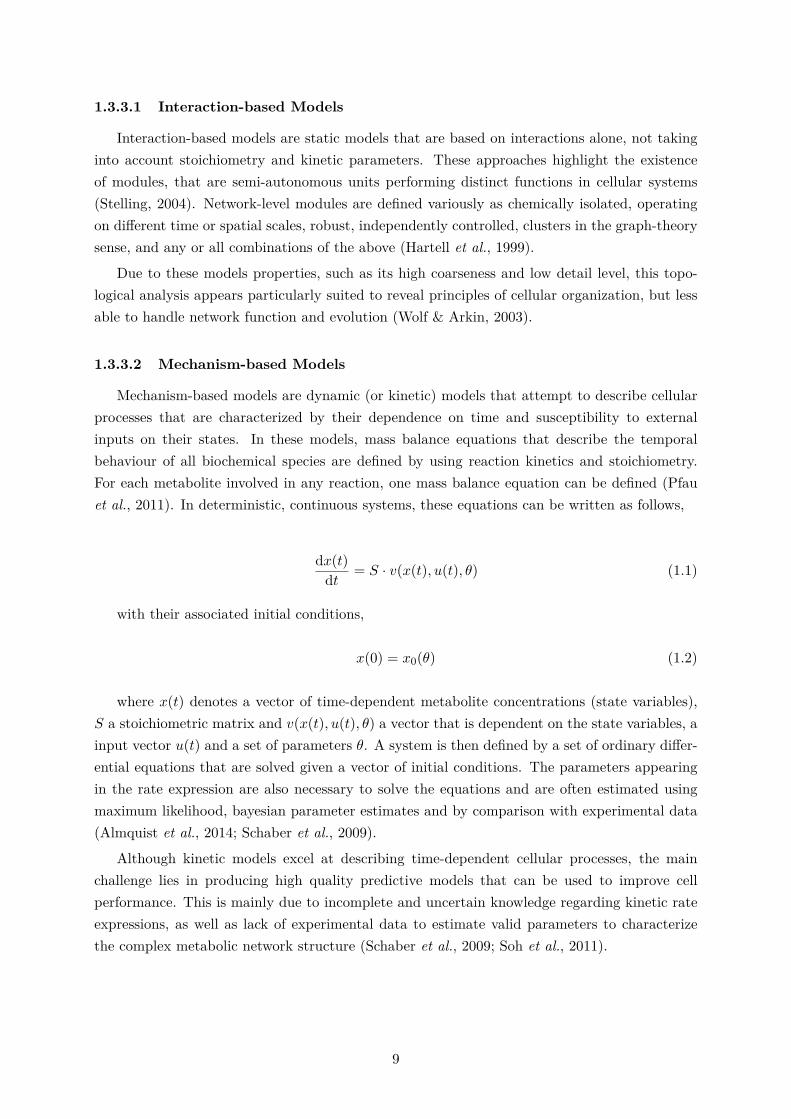
Mathematical modelling is able to generate experimentally testable hypotheses on underlyingmechanisms as well as predictions of cellular behaviour, thereby iteratively producing refinedmodels and insight into the system (Kitano, 2002). It comprises several approaches to representreality that ranges from global, yet coarse, views of cellular systems to detailed descriptions witha more limited scope. There are three main approaches to the mathematical modelling of cellularnetworks: (1) interaction-based models that are based on interactions alone; (2) constraint-based models that include constraints such as network topology, stoichiometry and reactionreversibilities; and (3) mechanism-based models where detailed reaction mechanisms andparameters are added (Stelling, 2004). A schematic summary of these mathematical modellingapproaches is shown below in Figure 1.5.

7

Figure 1.5: Cellular networks mathematical modelling approaches. In the top row, some key features ofeach method are presented. Schemes in the bottom row illustrate typical analysis results, namely (a) hubs(red circles) in a scale-free interaction network, (b) the cone of admissible flux distributions in a metabolicnetwork constructed from the metabolic pathways (edges), and (c) dynamics in the concentrations ofcellular components along time (From Stelling, 2004).

These methods will be discussed in the following subsections at a detailed level. Nevertheless,it is important to keep in mind that none of the approaches have the capability to cover the entirenetwork complexity while maintaining a high level of detail and accuracy. However, mechanism-based modelling is the most obvious candidate for achieving a system-wide understanding; yet,it is not possible to scale to a complete genomic level (Figure 1.6).

Figure 1.6: Mathematical modelling: scope and interactions. The three methods of modelling ap-proaches are positioned according to the achievable degree of detail and accuracy, and the typical net-work sizes they can handle (network complexity). Black arrows refer to possible interactions. The greenvertical arrow indicates the desirable progress towards genome-scale, mechanism-based models that allowfor a system-level understanding from the genotype. Boxes and arrows in light colours visualize thecontributions from all three approaches (From Stelling, 2004).

8

1.3.3.1 Interaction-based Models

Interaction-based models are static models that are based on interactions alone, not takinginto account stoichiometry and kinetic parameters. These approaches highlight the existenceof modules, that are semi-autonomous units performing distinct functions in cellular systems(Stelling, 2004). Network-level modules are defined variously as chemically isolated, operatingon different time or spatial scales, robust, independently controlled, clusters in the graph-theorysense, and any or all combinations of the above (Hartell et al., 1999).

Due to these models properties, such as its high coarseness and low detail level, this topo-logical analysis appears particularly suited to reveal principles of cellular organization, but lessable to handle network function and evolution (Wolf & Arkin, 2003).

1.3.3.2 Mechanism-based Models

Mechanism-based models are dynamic (or kinetic) models that attempt to describe cellularprocesses that are characterized by their dependence on time and susceptibility to externalinputs on their states. In these models, mass balance equations that describe the temporalbehaviour of all biochemical species are defined by using reaction kinetics and stoichiometry.For each metabolite involved in any reaction, one mass balance equation can be defined (Pfauet al., 2011). In deterministic, continuous systems, these equations can be written as follows,

dx(t)dt = S · v(x(t), u(t), θ) (1.1)

with their associated initial conditions,

x(0) = x0(θ) (1.2)

where x(t) denotes a vector of time-dependent metabolite concentrations (state variables),S a stoichiometric matrix and v(x(t), u(t), θ) a vector that is dependent on the state variables, ainput vector u(t) and a set of parameters θ. A system is then defined by a set of ordinary differ-ential equations that are solved given a vector of initial conditions. The parameters appearingin the rate expression are also necessary to solve the equations and are often estimated usingmaximum likelihood, bayesian parameter estimates and by comparison with experimental data(Almquist et al., 2014; Schaber et al., 2009).

Although kinetic models excel at describing time-dependent cellular processes, the mainchallenge lies in producing high quality predictive models that can be used to improve cellperformance. This is mainly due to incomplete and uncertain knowledge regarding kinetic rateexpressions, as well as lack of experimental data to estimate valid parameters to characterizethe complex metabolic network structure (Schaber et al., 2009; Soh et al., 2011).

9

1.3.3.3 Constraint-based Models

Constraint-based Models (CBMs) are static models where reactions stoichiometry and re-versibility constraints are added to the network topology. This deals with the lack of kineticinformation as these characteristics are largely available for metabolic networks (Szallasi et al.,2010).

CBMs core idea is to incorporate physicochemical and biological constraints that limit theoverall network behaviour and possible flux patterns confining the cellular phenotype to a set offeasible states (Orth et al., 2010). Metabolism usually involves fast reactions and high turnoverof substances. Therefore, it is assumed that, in longer time scales, metabolite concentrationis stable meaning that the rates at which a metabolite is produced and/or consumed becomeconstant over time. This generates an assumption that the system is time-invariant and insteady-state (Szallasi et al., 2010). Applying this assumption to Equation 1.1 leads to:

dx(t)dt = 0 (1.3)

and therefore,

S · v = 0 (1.4)

where v is no longer dependent on u(t) and θ as it is in Equation 1.1 as these models donot account for kinetic rates. One trivial solution to this equation is v = 0 that representsthermodynamic equilibrium. However, one is looking for the remaining non-obvious solutions.Given a stoichiometric matrix S with m×n dimensions, usually there are more reactions n thanthe number m of internal metabolites. Consequently, this system will be undetermined (m ≤ n)and all possible solutions are contained in a vector space called the null-space (or kernel) of S.Any point in this space can be described by a vector v ∈ Rn which is called a solution or fluxdistribution (Orth et al., 2010).

Moreover, additional constraints can be added that are expressed by linear equations orinequalities. Regarding reaction capacity, one can define a range of acceptable flux values foreach reaction. This is done by adding a upper bound ubi and a lower bound lbi to a reaction i,which will impose a maximum and minimum value, respectively.

lbi ≤ vi ≤ ubi (1.5)

Capacities can also be translated in reaction reversibilities. If a reaction i is consideredirreversible then lbi ≥ 0, whereas if lbi < 0 the reaction is reversible. When there is no knowledgein regards to capacities the reaction rates limits are set to ±∞.

It is important to note that, if there is exact knowledge and measurements mi of a flux

10

rate then vi = mi. This allows a reduction of degrees of freedom and, consequently reducesthe solution space (Szallai et al., 2010). An overall representation of CBMs is presented inFigure 1.7.

Figure 1.7: Principles of the stoichiometric modeling framework. Given a metabolic network, themass balance around each intracellular metabolite can be mathematically represented with an ordinarydifferential equation. If we do not consider intracellular dynamics, the mass balances can be described bya homogeneous system of linear equations. Other constraints can be also incorporated to further restrictthe space of feasible flux states of cells (Adapted from Estrada, 2010).

1.4 Phenotype Prediction

1.4.1 Flux Balance Analysis

Flux Balance Analysis (FBA) is a widely used phenotype prediction method to study bio-chemical networks. It calculates the flow of metabolites through a metabolic network, findingbiologically relevant solutions whether by predicting the growth rate of an organism or themaximum production of a biotechonologically relevant product (Orth et al., 2010).

To formulate a FBA problem, the first step is to mathematically represent the metabolicnetwork. This is done by constructing a stoichiometric matrix that imposes constraints on theflow of metabolites through the network. Furthermore, additional constraints are added such asinequalities that impose boundaries in the system. Lastly, a linear objective function is requiredto solve the FBA problem. The latter function is defined by choosing a relevant biologicalobjective in the study (Orth et al., 2010). For example, in the case of growth prediction, theobjective is biomass production, whereas in the case of product prediction, the objective is thereaction that produces it. Mathematically, an objective function is used to quantitatively definehow much each reaction contributes to the phenotype and can be formulated as

Z = cTv (1.6)

where c is the coefficient vector that defines the contributing weight of each flux in theobjective function (Pfau et al., 2011).

11

The metabolic network mathematical representation together with the objective define asystem of linear equations, whose optimization problem can be generally solved using linearprogramming (LP) (Szallasi et al., 2010). The general formulation for a simple FBA optimizationproblem is given as follows:

maxv

Z = f(v)

s.t. S · v = 0

lbi ≤ vi ≤ ubi

(1.7)

A summary representation of a FBA problem characterization is given below in Figure 1.8.

Figure 1.8: The conceptual basis of a FBA problem. With no constraints, the flux distributions maylie at any point in the solution space. When constraints are imposed by the stoichiometry matrix S andby the lower and upper bounds it defines an allowable solution space. Finally, through optimization ofan objective function, a single optimal flux distribution can be determined that lies on the edge of theallowable solution space (From Orth et al., 2010).

1.4.2 Flux Variability Analysis

The optimal solution to a FBA problem is rarely unique as there are other equally optimalexisting solutions in the solution space. Flux variability analysis (FVA) is a derivative fromFBA that aims to identify maximum and minimum fluxes through a reaction given an objectivevalue, returning flux boundaries for each reaction.

Each flux is maximized and minimized and these objective values correspond to the truereaction limits in the metabolic network. Each reaction flux is computed using a double linearprogramming problem, meaning there is a maximization and a subsequent minimization, andthese values correspond to the flux range in the metabolic network,

min/maxv

vi

s.t. S · v = 0

lbi ≤ vi ≤ ubi

(1.8)

where vi is the solution space for a reaction where vmax and vmin are calculated, containingthe maximum and minimum feasible flux values, respectively (Gudmundsson & Thiele, 2010).

Reactions that present a low flux variability are more likely to be of a higher importanceto the organism. Thus, FVA can be a promising technique for identifying important reactionsand/or pathways in the model (Muller & Bockmayr, 2013).

12

1.4.3 Parsimonious Enzyme Usage FBA

Parsimonious enzyme usage FBA (pFBA) is a derivative from FBA where a second layerof optimization criteria is added making it a bilevel linear programming problem. It relieson the minimization of gene-associated protein cost while maintaining optimal growth. ThepFBA optima represents set of genes associated with maximum growth as well as minimum-fluxsolutions, thereby predicting the most stoichiometrically efficient pathways.

This approach finds a flux distribution with minimum absolute values among the alterna-tive optima, assuming that the cell attempts to achieve the selected objective function whileallocating the minimum amount of resources (i.e. minimal enzyme usage).

1.5 Pathway Analysis

Pathway Analysis methods (PA), in contrast to methods such as FBA, are able to identify allmetabolic flux vectors without imposing any objective function. Instead, they characterize thecomplete space of admissible steady-state flux distributions by functional/structural units alter-nately to searching specific flux vectors. Thus, PA attempts to provide an unbiased perspectiveof the theoretical limits of the network as a whole.

1.5.1 Nullspace Analysis

The nullspace is characterized by the kernel matrix K containing columns of linearly inde-pendent vectors that satisfy the condition given by Equation 1.4. Each column from this matrixis a basis vector that generates the complete solution space (Pfau et al., 2011). From linearalgebra rank-nullity theorem, it is possible to find the number of columns by determining thenullity of K using Equation 1.9.

nullity(S) = n− rank(S) (1.9)

where n is the number of reactions in the system. Additionally, any flux distribution validfor Equation 1.4 can be constructed through linear combination of the columns from K,

r = K · b (1.10)

where b is a vector with the weight of each column in K.

Analysing the K matrix one can retrieve important information such as blocked reactionsand enzyme subsets. Blocked reactions can be identified if their corresponding row i in K isa zero row. This is helpful since these reactions hardly have any function in the system andmay be removed for practical reasons. Enzyme subsets (ES) (or coupled/correlated reaction set)are set of reactions that must operate together with a fixed reaction rate ratio. These can beidentified from the null space matrix as the corresponding rows in K of a set of reactions from

13

the same ES can only differ by a scalar factor α,

vi = α · r, i = 1, ..., n (1.11)

where vi is the reaction rate vector for reaction i. These reactions are therefore linearlydependent (Szallasi et al., 2010).

In nullspace analysis, thermodynamic constraints are not applied and thus, it is necessaryto be careful when aiming for biologically relevant results as some proprieties, such as reactionreversibilities, are unconstrained and may be transgressed.

1.5.2 Convex Analysis

In convex analysis, contrarily to nullspace analysis, in addition to steady-state assumption,thermodynamic constraints are applied and the space of feasible flux distributions can be definedas follows,

P = {v ∈ Rn : S · v = 0 ; I · v ≥ 0} (1.12)

where S is a m× n stoichiometric matrix, v a possible solution in the admissible space andI a diagonal n× n matrix with I ii = 1 if the flux i is irreversible (otherwise is 0).

This is a subset of the nullspace of S and in geometrical terms, this space of admissible fluxdistributions P , is a pointed convex polyhedral cone. This cone has a finite number of edgesand is located in the positive orthant Rn

+. By being convex, any vector within the cone (feasiblesolution) can be generated by non-negative linear combination of the vectors that generatedthe cone (which correspond to its edges) (Llaneras & Pico, 2010; Klamt et al., 2017). A visualexample of a convex polyhedral cone is given below in Figure 1.9.

Figure 1.9: Representation of a pointed convex polyhedral cone for a metabolic network with threereactions (V1, V2 and V3). The admissible solution space (highlighted in grey) has positive or nullreaction rates since it is strictly in the positive orthant R3

+. The edges (E1-E5) define the cone and canbe used to describe any feasible flux distribution through linear combination. The cone basis representsthe optimal solution space, obtained when using constraint-based approaches (Adapted from Papin etal., 2002).

14

1.5.3 Elementary Flux Modes

Elementary Flux Modes (EFM) are flux distributions that are calculated by solving Equa-tion 1.4 in conjunction with thermodynamic feasibility (Equation 1.12) and non-decomposabilityconstraints. The support function supp(v) provides a set of reaction indices from v with thecondition that a reaction i can only be a part of supp(v) if it has a nonzero flux value (vi 6= 0).Any elementary mode e is unique and minimal, in the sense that no reaction carrying a fluxcan be removed without violating the solving conditions. If a set of reactions constitutes anEMF then it fulfills the following proprieties (Schuster & Hilgetag, 1994; Schilling et al., 2000;Schuster et al., 2002):

• Pseudo steady state: According to Equation 1.4, no metabolite is consumed or producedin the overall stoichiometry. Hence, EFMs must belong to the nullspace of S.

• Feasibility: All fluxes have to be thermodynamically feasible and abide to their reactionreversibility. Hence, formally it requires that all rates vi ≥ 0 if reaction i ∈ irrev.

• Non-decomposability: This is the central property of EFMs and states that these fluxdistributions (or modes) represent the minimal functional units in a network. Hence, noreaction with a non-null flux value can be deleted from it, while still yielding a valid fluxpattern. This feature is also known as genetic independence as this condition implies thatthe participating enzymes in one pathway are not a subset in another pathway.

• If e is an elementary flux mode, so is any f = k · e with k > 0.

• Every valid flux distribution v can be generated through linear combinations of supportvectors that describe EFMs and/or scalars. These define the relative weight of each EFMin the flux distribution vector.

• Considering a set E of EFMs and a flux distribution vector v defined by Equation 1.13where w is a vector with the relative weight of each EFM. If the EFMs in E are valid,supp(E) can not contain reaction indices that are not already contained in supp(v).

v = w · E ; w ∈ R|E|0+ (1.13)

In sum, each EFM can be defined as a unique, minimal set of reactions that support steadystate operation of a metabolic network with irreversible reactions to proceed in appropriate di-rections (Trinh et al., 2009). Thus, EFMs can be interpreted as the most elementary pathwaysof a metabolic system and are capable of providing concise information about the metabolic net-work, because they describe the possible (simplest) modes of operation of a system (Zanghelliniet al., 2013). The EFMs for a simple reaction network are shown in Figure 1.10.

15

Figure 1.10: Simple example of a biochemical network and its elementary flux modes. The networkconsists of three metabolites (A, B and C), three internal reactions and three exchange reactions (a),and there are four elementary modes (b). The flux directionality is represented by black arrows, whereasreactions that do not have flux are represented by blue arrows. (Adapted from Papin et al., 2004)

In the model, an EFM includes at least one input and one output that can be called netconversion. Identifying all the EFMs present in a model can be useful to identify which net con-version has the highest efficiency and which products are formed under each substrate. Similarly,EFMs performing undesired net conversions can also be identified (Pfau et al., 2011; Zanghelliniet al., 2013). For instance, from the biochemical network from Figure 1.10, one can see thatEFM2 and EFM4 have metabolite B as a product but what differs is the substrate, being A andC, respectively. This may be an indicator that this metabolic network is more robust when itcomes to produce metabolite B.

Some of the most interesting applications of EFM analysis in Metabolic Engineering are:(1) identifying all range of possibles substrates and products, as well as finding ideal pathwaysto essentially modify and improve a desired metabolic capability (Szallasi et al., 2010); (2)establishing the relative importance of a given reaction in a pathway. The higher number ofEFMs that have the same reaction involved, the higher the likelihood of that reaction beinga critical element to the metabolic system (Schuster & Hilgetag, 1994); and (3) measuringa pathway robustness through quantification. The number of EFMs that perform a given netconversion can be used as estimator to the pathway robustness (Szallasi et al., 2010).

1.5.4 Minimal Cut Sets

Minimal Cut Sets (MCS) are a complementary concept to EFMs. A cut set is a set of reac-tions that need to be removed to inactivate a specified target reaction or, in another perspective,reactions whose deletions leads to network failure (considering a target reaction). A cut set be-comes a MCS and is minimal in the sense that removing any subset of it from the network isnot sufficient to maintain the target reaction inactivation. This means that by removing onereaction from the MCS prevents it from being a cut set anymore (Klamt & Gilles, 2004; Clark& Verwoerd, 2012).

16

To illustrate the MCS concept, consider the example network shown in Figure 1.11.

Figure 1.11: Biochemical network example. The network consists of six metabolites (A, B, C, D, Eand X) and nine reactions (R1, R2, R3, R4, R5, R6, R7, R8 and R9) (Adapted from Klamt & Gilles etal., 2004).

Assuming that one wants to block the production of metabolite X, a trivial solution is tocut the target reaction (R9 ) itself. However, it is not a biological reasonable strategy as R9 isan exchange flux (pseudo-reaction) and, therefore, might not have the corresponding genes tobe candidates for deletion. To find all MCSs that block R9, the minimal set of reactions thatdisable all EFMs must be found (Klamt & Gilles, 2004; Klamt, 2006). The set of EFMs andMCSs that block R9 in the network depicted in Figure 1.11 are in Figure 1.12.

Figure 1.12: Elementary modes and minimal cut sets that block R9 from the network in Figure 1.11.Elementary flux modes that carry flux through R9 are highlighted in grey. (Adapted from Klamt &Gilles et al., 2004).

17

Another example is MCS5, where R5 and R8 are deleted. This cut set is sufficient enoughto prevent production of X. Moreover, removing only R5 or only R8 will allow the flux togo through R9 again. Thus, this cut is a MCS because no subset of {R5,R8} would be asubset anymore. If there was a new subset, one would have a sub-optimal cut set instead ofa minimal cut set. Additionally, MCS2 is the only cut set with one reaction (apart from thetrivial solution). This could be an excellent suitable candidate since it seems to be essential tosynthesize metabolite X (Klamt & Gilles, 2004; Klamt, 2006).

In a Metabolic Engineering context, MCSs are useful to predict sets of genes which shouldbe knocked out in order to inactivate a particular metabolic reaction based on the smallest setof reactions to achieve this goal. Alternatively, in a scenario where a given metabolite is desiredto be produced it is feasible to calculate the MCS using additional constraints (Klamt & Gilles,2004; Clark & Verwoerd, 2012).

A limitation to using MCSs is that they might disable not only undesired reactions but alsodesired functions. For instance, one MCS may block the synthesis of an undesired product, whileat the same time removing the substrate uptake for a reaction where a metabolite of interest isbeing produced. To account for the need of keeping some reactions/EFMs intact, the conceptof constrainted MCS (cMCS) can be introduced. Formally, a set of desired EFMs , D, is definedalongside a set of undesired modes (target), T. An admissible MCS is reached when all targetmodes T are hit, while preserving a minimum number n of desired EFMs. This results in a setof reactions ready to be deleted from the network and that are still guaranteed to provide thedesired functionalities (Hadicke & Klamt, 2011).

1.6 Motivation and Objectives

This thesis has its starting grounds on a previous study done by Pandey et al. (2018). In thisstudy, an E. coli type K-12 phosphoglucose isomerase (∆pgi) mutant strain was transformed witha plasmid coding for IFNγ and tested for its expression capabilities, plasmid copy number andmRNA coding for IFNγ number. In addition, a detailed network comprising 100 metabolites and114 reactions of the central carbon metabolism of this strain was constructed. Then, elementarymode analysis was performed to check flux efficiency from pgi mutation and it was predictedthat the mutant would have a higher efficiency towards plasmid and protein synthesis. Thishypothesis was corroborated experimentally as there was a 3.0-fold increase in IFNγ in the ∆pgimutant.

At the same time, in a work done by Vieira (2015), a generic pipeline for enumerationof minimal cut sets in stoichiometric metabolic models (based on MCSEnumerator algorithm(Kamp & Klamt, 2014)) was implemented and validated. These types of algorithms are relevantin this work as they enable the possibility to enumerate knockouts in a more efficient andsimplified manner. Without these methods, enumerating MCSs would be very demanding andwould require high computation power even to compute lower sized knockout solutions.

Bearing this in mind and combining these two works together, the main objective of thisthesis is to apply minimal cut sets algorithm to find solutions for the optimal and efficient plasmid

18

and recombinant protein production. In the present work, IFNγ was used as the recombinantprotein to apply the MCS algorithm developed by Vieira (2015). IFNγ is a dimerized solublecytokine that plays a critical role in innate and adaptive immunity against mainly viral infections.Besides its ability to inhibit viral replication, IFNγ plays a big role in the immune system withits immunostimulatory and immunomodulatory effects. As a therapeutic agent, this proteincan be used to treat chronic granulomatous disease, that is a condition in which cells of theimmunity system have difficulty forming superoxide radical to kill certain pathogens.

Furthermore, the central carbon metabolic network developed by Pandey (2018) and agenome-scale E. coli K-12 metabolic network were used. To these models, plasmid, recom-binant protein and resistance marker production reactions were formulated in four differentways and added. Then, different MCS enumeration problem formulations were constructed andapplied to these models.

Lastly, all the results from both models were analysed with the objectives of: (1) corrob-orating the findings from Pandey et al. (2018) that E. coli pgi mutant increases plasmid andrecombinant protein production flux efficiency; and (2) identifying a possible new knockout orset of new knockouts strategies that would lead to a more optimal and efficient plasmid and/orrecombinant protein production and that are biologically relevant and feasible.

19

20

Chapter 2

Materials and Methods

In this Chapter, the methodology used in the practical part of this work is described. Em-phasis on the framework and mathematical algorithms is added.

2.1 Metabolic Models

All metabolic models that were used to perform simulations and their characteristics aredetailed in the following sections.

2.1.1 Central Metabolism Model

The Central Metabolism Model (CMM) used throughout this work has its foundation in amodel constructed by Pandey et al., 2018. It is a small detailed network of the E.coli centralcarbon metabolic pathway. This network comprises 100 metabolites and 114 reactions (AppendixA), where 9 are exchange and 17 are reversible (the remainder are internal and irreversiblereactions). From the list of metabolites, only seven are considered external, those being glucose,ammonium, phosphate, oxygen, carbon dioxide, ethanol and acetate. Glucose is consideredthe sole carbon source whose cell uptake is done via the phosphotransferase system (PTS).Simultaneously, ethanol and acetate are the overflow metabolites secreted that are produced bythe cell to balance the NADH/NAD+ pool and obtain extra ATP under high carbon sourceuptake rate or low oxygen availability, which is normal during batch growth. Once secreted,these metabolites can be consumed back, thus the glyoxylate cycle, gluconeogenesis and Entner-Doudoroff (ED) pathways were added. The synthesis of nucleotides and amino acids, essentialto biomass production, were also included separately. As for transhydrogenase activity, E.coli isknown for having two transhydrogenases, that are represented in this network by two reactionswith a cost of 0.25 mole ATP per mole of produced NADH. Regarding energy balance, on theone hand, maintenance energy requirements were addressed by including an ATP hydrolysisreaction. On the other hand, for ATP regeneration via oxidative phosphorylation, both NADHand FADH were considered separately with a yield of 2 and 1 mole of ATP on one mole ofNADH and FADH, respectively. Furthermore, biomass pseudo reaction was constructed withamino acids, nucleotides, lipids and other requirements. Recombinant proteins and plasmids

21

were synthesized using amino acids and nucleotides, respectively, accounting energy expenditures(further details in Section 2.1.3 - Model Formulations).

2.1.2 Genome-scale Model

The Genome-scale model (GSM) used throughout this work was iJO1366, whose reconstruc-tion was done by Orth et al., 2011. It is an extremely detailed network that is representativeof the E. coli K-12 MG1655 metabolism and that was expanded from a previous model, theiAF1260. The updated version of this network was obtained from BiGG Models databaseand presently accounts for 1367 associated genes, 2585 metabolic reactions and 1805 metabo-lites. Unlike CMM, these metabolites and reactions can be compartmentalized in cytoplasmic,periplasmic or extracellular, adding another level of complexity. Additionally, this model has 39subsystems, from which alanine and membrane lipid metabolism to glycolysis/gluconeogenesisand tricarboxylic acid (TCA) cycle, are just some examples. Recombinant proteins and plas-mids synthesis were added to the model using amino acids and nucleotides, respectively, andaccounting energy expenditures that are further detailed in the following Section 2.1.3.

2.1.3 Model Formulations

In model formulations, the objective was to construct stoichiometric reactions for the syn-thesis of a plasmid, its resistance marker and a recombinant protein. Additionally, differentprotein producing metabolic networks and ways to formulate the enumeration problems weredeveloped.

Recombinant Protein

Regarding the recombinant protein synthesis, the selected model protein for this work was thehuman interferon gamma (IFNγ) as studied by Pandey et al., 2018. This synthesis reaction wasincluded by quantifying the per mole amino acid requirement for the His-tagged IFNγ (AppendixB) and assuming 4.3 ATPs per peptide bond as it is, approximately, the necessary energy tocondensate two amino acids. Protein primary sequence and composition is available at NCBIdatabase reference sequence number NP 000610.2 (Interferon gamma precursor [homo sapiens])and to this sequence, a 6 histidines His-tag was added to perform stoichiometric computations,consistent with the protein produced experimentally by Pandey et al.(2018).

Plasmid

For plasmid synthesis, the selected model plasmid for this work was the pET28a vectorsystem from Novagen as used by Pandey et al., 2018. This synthesis reaction was included byquantifying the per mole deoxyribonucleotide triphosphate (dNTP) requirement for the pET28a-IFNγ system (considering the His-tag) (Appendix B). The necessary energy to condensate twodNTPs was assumed to be approximately 1.36 ATPs per nucleotide bond. Plasmid primarysequence and composition is available at Addgene database and to this sequence, a nucleotidic

22

IFNγ sequence that is available at NCBI database accession reference AB451324.1 was addedto perform stoichiometric computations.

Resistance Marker

A resistance marker synthesis reaction was added based on the plasmid antibiotic resistance.The pET28-a vector system presents a kanamycin resistance marker and thus a reaction wasincluded quantifying the per mole amino acid requirement for the production of the enzyme thatconfers resistance to kanamycin (aminoglycoside O-phosphotransferase APH(3’)-Ia). The energyexpenditures were assumed to be 4.3 ATPs per peptide bond and the primary sequence andcomposition of this phosphotransferase was obtained from NCBI database reference sequencenumber WP 000018329 (aminoglycoside O-phosphotransferase APH(3’)-Ia [Bacteria] (kanR)).

Model Configurations

In addition to the metabolic reactions present in the models, different ways to balance theequations of plasmid and/or IFNγ synthesis were considered, giving rise to different ways torepresent the E. coli K12 system. In total 4 different balance equation formulations were createdand all the changes to both models (CMM and GSM) were done in MATLAB using COBRAToolbox.

The base model is the simplest and comprises only a reaction to account for plasmid syn-thesis. It does not contain in its stoichiometric matrix any information regarding IFNγ andphosphotransferase. Thus, this model is built on an assumption that plasmid and recombinantprotein production are directly proportional, meaning that the more plasmids there are, themore recombinant proteins will be translated from those plasmids at a given time. Equation 2.1represents, without adequate stoichiometry, the reaction added to this model.

∑pET28a-IFNγ dNTPs + ATP→ Plasmid + ADP + Pi (2.1)

Moreover, another level of detail was added to the previous base model. A IFNγ synthesisreaction was added and is independent from the plasmid reaction. This model treats bothplasmid and recombinant protein as uncorrelated entities. From this model, it can be interestingto visualize the flux to one product or another since their monomers’ origin is metabolicallydistinct. The following Equation 2.2 represents the new reaction added.

∑IFNγ amino acids + ATP→ IFNγ + ADP + Pi (2.2)

For the third model, a resistance marker synthesis reaction was joined to the previous model.This reaction is independent from the plasmid and IFNγ reaction, only relying on its primaryamino acid sequence as precursors. All the entities are uncorrelated and independent from eachother. From this model, it can be interesting to investigate how the system behaves and what

23

options are available when constraints are imposed.

∑Phosphotransferase amino acids + ATP→ Phosphotransferase + ADP + Pi (2.3)

Regarding the fourth and last model, a different approach was investigated. In this model,all the reactions are correlated with each other, meaning that IFNγ and phosphotransferase pro-duction are directly dependent on plasmid availability. In turn, plasmid availability is dependenton dNTPs as described in Equation 2.1. In addition, IFNγ and phosphotransferase depend onamino acids availability as described in Equations 2.2 and 2.3, respectively. Hence, for this pur-pose, and since there is not available information on ratios such as recombinant protein formedper plasmid, it was assumed that 1 mole of plasmids would give rise to 1 mole of IFNγ and 1mole of phosphotransferase, as represented by Equation 2.4.

1 Plasmid pET28a → 1 IFNγ + 1 Phosphotransferase (2.4)

From a biological standpoint this is the closest to reality since there is a correlation betweenproducts. However, from a computational point of view, it may not work as intended as it ismetabolically heavy for the network to mathematically allocate all these fluxes while maintainingbiomass growth. Table 2.1 summarizes all the models previously described, as well as a key thatwill be used throughout this work to simplify the analysis when referring to each model.

Table 2.1: Model configuration key and main aspects summary based on the previously describedbalance equations.

Model Equations Comment

A Eq. 2.1 Plasmid production. Base model with simplest configuration.

BEq. 2.1

Eq. 2.2Plasmid and IFNγ production. Independent reactions.

C

Eq. 2.1

Eq. 2.2

Eq. 2.3

Plasmid, IFNγ and phosphotransferase production. Independent reactions.

D Eq. 2.4 IFNγ and phosphotransferase production dependent on plasmid availability.

24

Problem Configurations

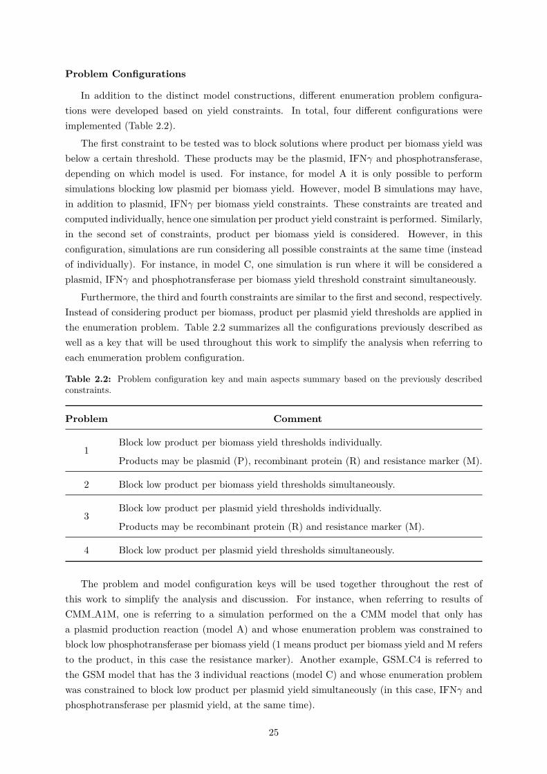
In addition to the distinct model constructions, different enumeration problem configura-tions were developed based on yield constraints. In total, four different configurations wereimplemented (Table 2.2).

The first constraint to be tested was to block solutions where product per biomass yield wasbelow a certain threshold. These products may be the plasmid, IFNγ and phosphotransferase,depending on which model is used. For instance, for model A it is only possible to performsimulations blocking low plasmid per biomass yield. However, model B simulations may have,in addition to plasmid, IFNγ per biomass yield constraints. These constraints are treated andcomputed individually, hence one simulation per product yield constraint is performed. Similarly,in the second set of constraints, product per biomass yield is considered. However, in thisconfiguration, simulations are run considering all possible constraints at the same time (insteadof individually). For instance, in model C, one simulation is run where it will be considered aplasmid, IFNγ and phosphotransferase per biomass yield threshold constraint simultaneously.

Furthermore, the third and fourth constraints are similar to the first and second, respectively.Instead of considering product per biomass, product per plasmid yield thresholds are applied inthe enumeration problem. Table 2.2 summarizes all the configurations previously described aswell as a key that will be used throughout this work to simplify the analysis when referring toeach enumeration problem configuration.

Table 2.2: Problem configuration key and main aspects summary based on the previously describedconstraints.

Problem Comment

1Block low product per biomass yield thresholds individually.

Products may be plasmid (P), recombinant protein (R) and resistance marker (M).

2 Block low product per biomass yield thresholds simultaneously.

3Block low product per plasmid yield thresholds individually.

Products may be recombinant protein (R) and resistance marker (M).

4 Block low product per plasmid yield thresholds simultaneously.

The problem and model configuration keys will be used together throughout the rest ofthis work to simplify the analysis and discussion. For instance, when referring to results ofCMM A1M, one is referring to a simulation performed on the a CMM model that only hasa plasmid production reaction (model A) and whose enumeration problem was constrained toblock low phosphotransferase per biomass yield (1 means product per biomass yield and M refersto the product, in this case the resistance marker). Another example, GSM C4 is referred tothe GSM model that has the 3 individual reactions (model C) and whose enumeration problemwas constrained to block low product per plasmid yield simultaneously (in this case, IFNγ andphosphotransferase per plasmid yield, at the same time).

25

2.2 Cellular Constraints

To solve MCS and FBA problems, biological or physiochemical cellular constraints need tobe added to limit the solution space to achieve desirable phenotypes. As the main objective wasto evaluate the system behaviour, most cellular constraints are not extremely strict. Glucosemaximum uptake rate was set to 1000 mmol/g ·h as well as the maximum oxygen consumptionrate. These bounds do not have any physiological and biological meaning. However, this way,the model has more freedom to use its main substrate sources and it is possible to evaluatewhether producing a by-product (recombinant protein, for instance) is viable with cell growth.Moreover, the upper and lower bounds on cellular maintenance energy (ATPM reaction) wereleft at the empirical default of 8.39 mmol/g · h (Orth et al., 2010). In addition to the previousconstraints, a minimum biomass and product per substrate yield threshold were added. Notdesiring to constraint too much the problem formulation, these values were both set to 0.0001.These cellular constraints were maintained in all simulations in this work and are presented insummary in Table 2.3.

Table 2.3: Cellular constraints applied to all the simulations and models used throughout this work.

ConstraintValue

(mmol/g · h)Comment

Glucose 1000 Glucose maximum uptake rate set to not constraint too much the system

Oxygen 1000 Oxygen maximum uptake rate set to not constraint too much the system

Maintenance 8.39 ATPM reaction set to empirical value as requirement cell maintenance.

Biomass 0.0001 Biomass reaction minimum threshold

Product/Glucose 0.0001 Product per substrate minimum yield threshold

To perform FBA and pFBA simulations, the maximization of biomass growth was the electedobjective function as it is the most commonly used biological optimization goal.

2.3 Enumeration Algorithm

To compute the MCS/cMCS enumeration problems, a method developed by Vieira (2015)was provided. In this work, Vieira implemented in Java programming language a library con-taining routines for MCS enumeration that can be used from small networks to genome-scalemetabolic models. In this context, the pipeline constructed by Vieira and incorporating fourmain steps is depicted in Figure 2.1.

26

Figure 2.1: Generic pipeline for enumerating MCSs featured in Vieira (2015) work (From Vieira, 2015).

• Model setup: In this step, the model is imported and unbounded fluxes are removed toimprove numerical stability. In addition, pseudo-reactions are identified as they will notbe part of the solutions.

• Pre-processing: This steps aims to improve computational speed by reducing the net-work complexity. It is accomplished by removing blocked reactions that are found throughflux variability analysis (FVA) and network compression by lumping correlated reactions.This compression is based on the enzyme subset concept from nullspace analysis, whereeach enzyme subset is considered a single reaction.

• Problem setup: In this step, the enumeration problem is assembled and validated beforecontinuing. A group of desired and undesired phenotypes is constructed based on fluxbounds (acting as capacity constraints) and yield constraints (that forces the ratio betweentwo fluxes to a threshold). After defining the phenotypic space, problem feasibility isassessed.

• Enumeration: In this last step, the proper formulation is built in the pre-processed modeland solved. The K-shortest algorithm is used to compute the EFMs (Figueiredo et al.,2009) and the MCSEnumerator algorithm to enumerate the MCSs (Kamp & Klamt, 2014).Then, the MCSs are checked for feasibility in the desired conditions. Finally, solutions aredecompressed with simple combinatorics and MCSs that do not belong to the desiredphenotypic space are discarded, leaving only cMCSs.

The provided problem formulation script was modified, using Eclipse software, to accommo-date the desirable phenotypes for this work described in the previous sections.

27

2.4 Statistical Methods

2.4.1 Principal Component Analysis

Principal component analysis (PCA) is an unsupervised learning method that aims to reducethe high dimensionality of a dataset while retaining its variation, patterns and trends. Thisdimensionality reduction is achieved by defining new variables that are a linear combination ofthe original ones and, geometrically, are the orthogonal projection - the principal components(PC). It is done as such that the first PC has the largest possible variance (accounting for as muchof the variability in the data) and each succeeding component in turn has the highest variancepossible under the constraint that it is orthogonal to the preceding components (Ringner, 2008).

Firstly, the data may require some processing, such as its centralization and standardization,taking into consideration that PCA is sensitive to the relative scaling of the original variables.Then, a correlation matrix is computed, containing the correlation values between all pairsof variables. From this matrix, the eigenvectors and eigenvalues can be extracted, describingthe directions of patterns in data and the variance explained by these directions, respectively.Eigenvectors correspond then to the principal components and the eigenvalues to the varianceeach component explains (Smith, 2002; Ringner, 2008).

PCA is useful and very common in biology as it helps reduce the high dimensionality in,for instance, NGS data where the number of samples is significantly lower than the number offeatures (genes or transcripts). The samples can then be plotted according to their projectiononto each of the components, allowing the visualization of possible patterns and groups containedin it.

In this work, PCA was used with the purpose of searching for patterns in reaction fluxesand to group similar solutions, ultimately to reduce the solution pool size. Principal componentanalysis was implemented in R using the function PCA from the FactoMineR package (Hussonet al., 2017).

2.4.2 Cluster Analysis

Cluster analysis (or clustering) is an unsupervised learning methodology which means thereare no predefined data labels or classes. The main goal of these methods is to group a set ofobjects in such way that objects in the same group (called clusters) are more similar to each otherthan to those in other clusters. The similarity/dissimilarity is a key component in clustering asit is the main controlling factor when grouping data and it is typically expressed in terms ofdistance. For such calculations, a distance metric is required and it is chosen according to thefeatures and type of data available. The most popular metrics are the Manhattan and Euclideandistances that calculate the distance between data points as given by Equations 2.5 and 2.6 ,respectively (Rokach & Maimon, 2005).

d(i, j) =∣∣xi1 − xj1

∣∣+ ∣∣xi2 − xj2∣∣+ ...+

∣∣xip − xjp

∣∣ (2.5)

28

d(i, j) =√∣∣xi1 − xj1

∣∣2 +∣∣xi2 − xj2

∣∣2 + ...+∣∣xip − xjp

∣∣2 (2.6)

The appropriate clustering algorithm and parameter settings (including distance function,a density threshold or the number of expected clusters) depend on the data set and intendeduse. As such, cluster analysis is rather an iterative process of knowledge discovery and it isoften necessary to modify data preprocessing and model parameters until the results achieve thedesired properties.

Hierarchical Cluster Analysis

Hierarchical cluster analysis (HCA) is a method which seeks to build a hierarchy whereclusters have subclusters that are organized in a tree, and each node (clusters) is the union of itschildren (subclusters). It can fall into two categories: the agglomerative and divisive approach.

The agglomerative clustering methods are the most used and work in a ”bottom-up” manner.That is, each object is initially considered a single-element cluster (leafs) and at each step ofthe algorithm the two most similar clusters are merged into one single big cluster (nodes). Thisprocedure is iterated until a stopping criteria is met or all elements are joined in one single cluster(root). This allows the construction of a nested grouping of patterns, usually represented in adendrogram (Gan et al., 2007).

On the other hand, divisive clustering methods are essentially the inverse process of anagglomerative technique and work in a ”top-down” manner. In this case, at the start, all objectsare included in one single cluster (root). At each step of iteration, the most heterogeneous clusteris divided into two (nodes). This process is iterated until each object has its own single-elementcluster (leafs) (Gan et al., 2007).

In this type of clustering the clusters of a higher hierarchy level encompass all the objectsthat belong to the merged clusters from the lower level, which means that when an object isassigned to a certain cluster it is not possible to reassigned to another cluster. In Figure 2.2 thetwo HCA approaches described above are represented (Rokach & Maimon, 2005).

To compute the dissimilarity between two clusters of observations there are three popularmethods:

• Single linkage: It computes all pairwise dissimilarities between elements in cluster Aand elements in cluster B, and considers the smallest of these dissimilarities as a linkagecriteria.

min{d(x, y) : x ∈ A, y ∈ B} (2.7)

• Complete linkage: It computes all pairwise dissimilarities between elements in clusterA and elements in cluster B, and considers the maximum value of these dissimilarities asthe distance between the two clusters.

max{d(x, y) : x ∈ A, y ∈ B} (2.8)

29

• Average linkage: It computes all pairwise dissimilarities between elements in cluster Aand elements in cluster B, and considers the average of these dissimilarities as the distancebetween the two clusters. It is an in between to the last two methods.

1|A| · |B|

∑x∈A

∑y∈B

d(x, y) (2.9)

Hierarchical algorithms are suitable for dataset with arbitrary shape and is advantageous asit outputs a hierarchy, that is a structure that can be more informative cluster-wise when com-parison to unstructured sets of flat clusters returned in other algorithms. However, it presentshigh inability to adjust decisions, given the impossibility of reassigning the objects to differentclusters after their assignment. It is also very sensitive to outliers and is not suitable for verylarge datasets (Santini, 2016).

Figure 2.2: Representation of the agglomerative and the divisive HCA approach.

2.5 Tools and Software

2.5.1 The R Programming Language

All the analytical work described throughout this thesis was implemented in R programminglanguage, a free software environment for statistical computing and graphics. R provides agrand variety of not only statistical methods but also good graphical visualization and can beeasily extended using a wide range of available packages, thereby facilitating data analysis andvisualization (R Development Core Team, 2011). In order to run R, a user-friendly environment,RStudio, that is an integrated development environment (IDE) was used.

The main majority of graphics and data visualization displayed throughout this work weregenerated through the ggplot function from the ggplot2 package available for R (Wickham, 2009).

30

2.5.2 MATLAB

MATrix LABoratory (MATLAB) is a computing environment and programming languagefor algorithm development, data analysis, visualization and numerical computation. It allowsmatrix calculations, plotting of functions and data, creation of graphical user interfaces (GUI)and algorithms that can be implemented or used from a vast library of pre-built toolboxes.In addition, it is possible to interface with programs developed in different languages (C/C++,Java R©, .NET, Python, SQL, Hadoop and Microsoft R© Excel R©) which makes it possible to harnessthe unique strengths of each language for various purposes.

Throughout this work, MATLAB was used to manipulate and construct all the metabolicmodels that were simulated. All these changes were achieved using the COBRA Toolbox(Heirendt et al., 2018).

2.5.2.1 The COBRA Toolbox

The COnstraint-Based Reconstruction and Analysis (COBRA) Toolbox is a set of methodsand utilities integrated as a form of software package to provide easy access to core COBRAmethodologies. It provides methods for quantitative prediction of cellular phenotype and multi-cellular biochemical networks with constraint-based modelling. It implements an extended andcomprehensive collection of modelling methods, from reconstruction and model generation toprediction and analysis methods. The openCOBRA project has been developing, starting withtools for MATLAB that are currently at their third version (The COBRA Toolboox v3.0) andthat have been expanding to Python (COBRApy) and Julia (COBRA.jl) modules (Heirendt etal., 2018).

The COBRA Toolbox for MATLAB was used to deal with the model reconstruction andrefinement. This toolbox offers the processing of SBML (Systems Biology Markup Language)files of metabolic networks, as well as the capability of reading and writing. Model manipulationfunctions such as addReaction and addMetabolite were commonly used to add information tothe network regarding the synthesis of plasmids or recombinant proteins. Some functions werecalled to export the new models; however, this toolbox was not used to apply any phenotypeprediction or analysis algorithm.

2.5.3 The Java Programming Language

In order to run the Java scripts to perform flux distributions simulations (pFBA and FVA)and apply the necessary problem formulation modifications, a user-friendly integrated develop-ment environment (IDE), Eclipse, was used. This software contains a base workspace with anextensive plug-in system for further customization. It is primarily used to develop Java applica-tions but may be also used with other programming languages. For this work, Eclipse Oxygenversion, released on June 2017, was used.

31

32

Chapter 3

Results and Discussion

In this Chapter, the main results generated with the different models are presented, analyzedand discussed. Regarding the Central Metabolism Models (CMM), an exploratory data analysiswas performed with the aim of finding a small number of solutions for a further detailed networkanalysis. For the Genome-scale Model (GSM), only an exploratory data analysis was performedin order to evaluate differences comparing to the smaller model.

3.1 Central Metabolism Model

3.1.1 Data Processing

Data were generated for each enumeration problem (combinatorial model and problem con-figurations) as previously described in Chapter 2. A maximum knockout size of 5 was allowedand all the solutions were stored as sets of strings encoding reactions. For each generated solu-tion, a pFBA flux distribution was computed and stored in a matrix where each row is a solutionand each column encodes a reaction. Hence, each matrix entry represents a flux value for a givenreaction in a particular set of knockouts (solution).

Before analysing the data, a pre-processing step was performed in order to help reducing datahigh dimensionality. In this step, some solutions were filtered based on their set of knockouts.On one hand, solutions that were biologically irrelevant were removed. These are solutionsthat comprise one or more reactions regarding: (1) production, such as biomass, plasmid,recombinant protein and resistance marker reactions that are the objective of this work makingtheir removal meaningless; (2) energy, such as ATP maintenance and synthesis reactions thatare essential to cell survival; and (3) transport such as glucose exchange reaction that is assuredby the PTS system and are also vital to cells. Table 3.1 summarizes all the reactions that weretargets of this filtration step.

On the other hand, solutions that were computationally irrelevant were removed. These wereselected based on biomass-product coupled yields (BPCY) and combined reaction flux values,depending on each model and formulation available. For instance, it can be considered that,solutions whose BPCY was above zero or solutions that present a flux different from zero in

33

plasmid and recombinant protein reactions, at the same time, are the ones to be kept for furtheranalysis.

These filtration steps were applied to each model and formulation. After processing, eachformulation data corresponding to a model was concatenated and analyzed simultaneously.

Table 3.1: Biologically relevant reactions that were filtered in the CMM data processing step. Solutions(set of knockouts) that comprised one or more of these reactions were removed from further analysis.

Reaction Description

R BiomassProduction Biomass production reaction

R PlasmidProduction Plasmid production reaction

R RecProduction Recombinant protein production reaction

R ResProduction Resistance marker production reaction

R ATPM ATP Maintenance reaction

R ATPS1 ATP Synthesis reaction (NADH related)

R ATPS2 ATP Synthesis reaction (FADH2 related)

R PTS Glucose transport system

3.1.2 Exploratory Data Analysis

In order to understand the main characteristics of the data, some exploratory data analysismethods were applied. A Principal Component Analysis (PCA) was performed after data fil-tration and standardization with the objective of evaluating the main source of data variation.In addition, a hierarchical cluster analysis (HCA) was performed with the aim of reducing thesolution pool by grouping solutions that present different sets of knockouts reactions but showsimilar phenotypes. These methods were applied on the pFBA flux distribution data.

In the next Sections, these methods’ results will be presented and discussed for all the fourmodels, and each model with all its possible problem configurations.

3.1.2.1 Model A

Model A takes only into consideration the plasmid production reaction. Consequently, thereis only one way to compose the enumeration problem, which is by constraining low plasmidproduction per biomass yields (formulation 1P). From the initial 723 different solutions obtainedfor this problem, only 8.2% remained for further analysis after the processing step. Table 3.2summarizes the number of suggested knockouts in a solution (MCS Size) and the amount ofsolutions that have that size.

34

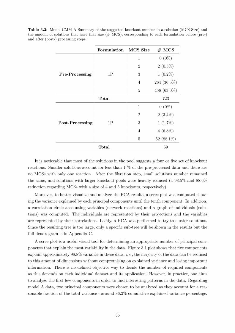
Table 3.2: Model CMM A Summary of the suggested knockout number in a solution (MCS Size) andthe amount of solutions that have that size (# MCS), corresponding to each formulation before (pre-)and after (post-) processing steps.

Formulation MCS Size # MCS

Pre-Processing 1P

1 0 (0%)

2 2 (0.3%)

3 1 (0.2%)

4 264 (36.5%)

5 456 (63.0%)

Total 723

Post-Processing 1P

1 0 (0%)

2 2 (3.4%)

3 1 (1.7%)

4 4 (6.8%)

5 52 (88.1%)

Total 59

It is noticeable that most of the solutions in the pool suggests a four or five set of knockoutreactions. Smaller solutions account for less than 1 % of the pre-processed data and there areno MCSs with only one reaction. After the filtration step, small solutions number remainedthe same, and solutions with larger knockout pools were heavily reduced (a 98.5% and 88.6%reduction regarding MCSs with a size of 4 and 5 knockouts, respectively).

Moreover, to better visualize and analyze the PCA results, a scree plot was computed show-ing the variance explained by each principal components until the tenth component. In addition,a correlation circle accounting variables (network reactions) and a graph of individuals (solu-tions) was computed. The individuals are represented by their projections and the variablesare represented by their correlations. Lastly, a HCA was performed to try to cluster solutions.Since the resulting tree is too large, only a specific sub-tree will be shown in the results but thefull dendrogram is in Appendix C.

A scree plot is a useful visual tool for determining an appropriate number of principal com-ponents that explain the most variability in the data. Figure 3.1 plot shows that five componentsexplain approximately 98.8% variance in these data, i.e., the majority of the data can be reducedto this amount of dimensions without compromising on explained variance and losing importantinformation. There is no defined objective way to decide the number of required componentsas this depends on each individual dataset and its application. However, in practice, one aimsto analyze the first few components in order to find interesting patterns in the data. Regardingmodel A data, two principal components were chosen to be analyzed as they account for a rea-sonable fraction of the total variance - around 86.2% cumulative explained variance percentage.

35

●

●

●

●● ● ● ● ● ●

64.8%

21.4%

8.2%3.4%1% 0.9%0.2%0% 0% 0%0

20

40

60

1 2 3 4 5 6 7 8 9 10Principal Components

Perce

ntag

e of e

xplai

ned

varia

nces

(%)

A)

R_GLUTS

R_NH3(e)R_UDPK

R_ASPOX

R_GLC(e)

R_PGM

R_FAS4R_PPI

R_PSP

R_UMPK

−1.0

−0.5

0.0

0.5

1.0

−1.0 −0.5 0.0 0.5 1.0Principal Component 1

Pri

nci

pal

Com

pon

ent

2

B)

WTsol_708sol_707sol_173sol_483sol_480sol_476sol_478sol_0sol_3sol_719sol_482sol_172sol_499sol_351sol_720sol_711sol_709sol_710

051015 Dendrogram Height

C)

−10

0

10

−5 0 5 10 15Principal Component 1

Pri

nci

pal

Com

pon

ent

2

D)

Figure 3.1: Model CMM A Exploratory data analysis results: A) Scree plot percentage of explainedvariances (%) in each principal component (up to a total of ten PCs); B) Correlation circle correlationbetween the top 10 variables contributing to the PCs and the first and second principal components; C)Dendrogram hierarchical cluster analysis performed using single linkage method and euclidean distancemetric. The sub-tree was obtained by a cut done at a dendrogram height equal to 15; D) Individualsgraph data projection coordinates in the first two principal components: CMM A1P.

A correlation plot gives the variables direction vectors and helps describing the strengthof relationship between two variables. A correlation coefficient ranges from -1 to +1, where+1 indicates a perfect positive linear relationship, and -1 a perfect negative linear relationship.Variables which have little contribution to a direction have almost zero weight. Drawing thisplot may contribute to understand, in general, which variables have positive and negative impacton the principal components. Strongly related variables, will be positively correlated, and inthis plot, will appear near each other. Meanwhile, negatively correlated variables will appeardiagonally opposite to each other. If two variables are unrelated, they will appear orthogonal toeach other. Additionally, the length of an arrow represents how well it explains the distributionof the data. A variable with a long arrow means it is better represented in the principal com-ponents. Figure 3.1 correlation circle shows the top ten contributing variables to the fist andsecond dimensions. From this plot, all arrows have a similar length, so the parameters contributeequally. Moreover, nine out of ten variables are strongly positively correlated, whereas R PGMis negatively correlated. The latter, corresponds to a reaction in gluconeogenesis where glucose-6-phosphate is transformed back to glucose for energy reservation. In this way, it is valid thatthis variable is negatively correlated as the remaining reactions are mostly essential to nucleotide

36

synthesis, where there is a high energy and substrate consumption, in contrast to R PGM whoseobjective is completely the opposite. Furthermore, some of the positively correlated reactionsconcern amino acid synthesis such as R PSP (serine synthesis) and R ASPOX (aspartate syn-thesis). Even though in this model there is not a reaction accounting for recombinant proteinproduction, these amino acids are essential for the pseudo biomass reaction. Additionally, theseare also fundamental early precursors in nucleotide synthesis for the plasmid production (serineis involved in MetTHF synthesis and aspartate in PRAIC synthesis). Overall, these top con-tributing variables show that there is high variation in reactions concerning nucleotide synthesiswhich is consequently related to plasmid production.

The individuals graph, also known as score plot, is a projection of the data scores intoprincipal components and it is used for finding and interpreting relationships between individ-uals/observations. It can be used to assess the data structure and detect clusters, outliers,and trends. Groupings of data on the plot may indicate two or more separate distributionsin the data. In this model, there is only one possible enumeration problem and, thus PCA isnot as helpful in pattern visualization as there are not any separations to be made. AlthoughPCA does not compute which solutions belong together, since to do that clustering methodsare needed, it can still give a good visualization of how individual solutions are grouped. Forinstance, from this score plot it is possible to say that an amount of solutions are very closelygrouped (highlighted by the strong pink coloured circle in the left, resulting of solution overlap-ping) and that contribute exclusively to the first dimension. These solutions may be a possiblecluster that could reduce the solution pool as they may represent the same phenotype. In thisgroup, most of the solutions have a MCS length of 5, where 4 suggested knockouts remain thesame (R TRANSH2, R ACK, R ADH and R SDH ) and the last reaction is different for eachsolution. These reactions are tightly related to overflow metabolites that are secreted by cells tobalance NADH/NAD+ and obtain ATP (R ACK for acetate and R ADH for ethanol), as wellas other cell mechanisms to balance reducing power such as R TRANSH2 for NADPH/NADHand R SDH for FADH2. In addition, these solutions have a similar phenotype to a smallersuggested 2 knockout solutions (R TRANSH2 and R PDH ) and, thus it may be an interestingtarget for a further detailed analysis to study and explain how a similar phenotype is achievedby deleting 2 reactions instead of 5.

A dendrogram is a tree diagram used to illustrate the arrangement of the clusters producedby hierarchical clustering, which is useful to find correlated groups. The horizontal axis of adendrogram represents the distance or dissimilarity between clusters, whereas the vertical axisrepresents the objects and clusters. Each joining (fusion) of two clusters is represented on thegraph by the splitting of a horizontal line into two horizontal lines. The horizontal positionof the split, shown by a short vertical bar, gives the distance (dissimilarity) between the twoclusters. Furthermore, cutting a dendrogram at a certain level/height gives a set of clusters.Thus, depending at which height the cut is done, one can have variable cluster numbers. There isno definitive height at which a dendrogram should be cut as the resulting hierarchical structure iscontext-dependent. Figure 3.1 shows a sub-tree that was obtained by cutting the full dendrogramat a height equal to 15. This tree was computed using single linkage method and euclideandistance as the metric distance. Since the main objective behind our HCA is to find solutions

37

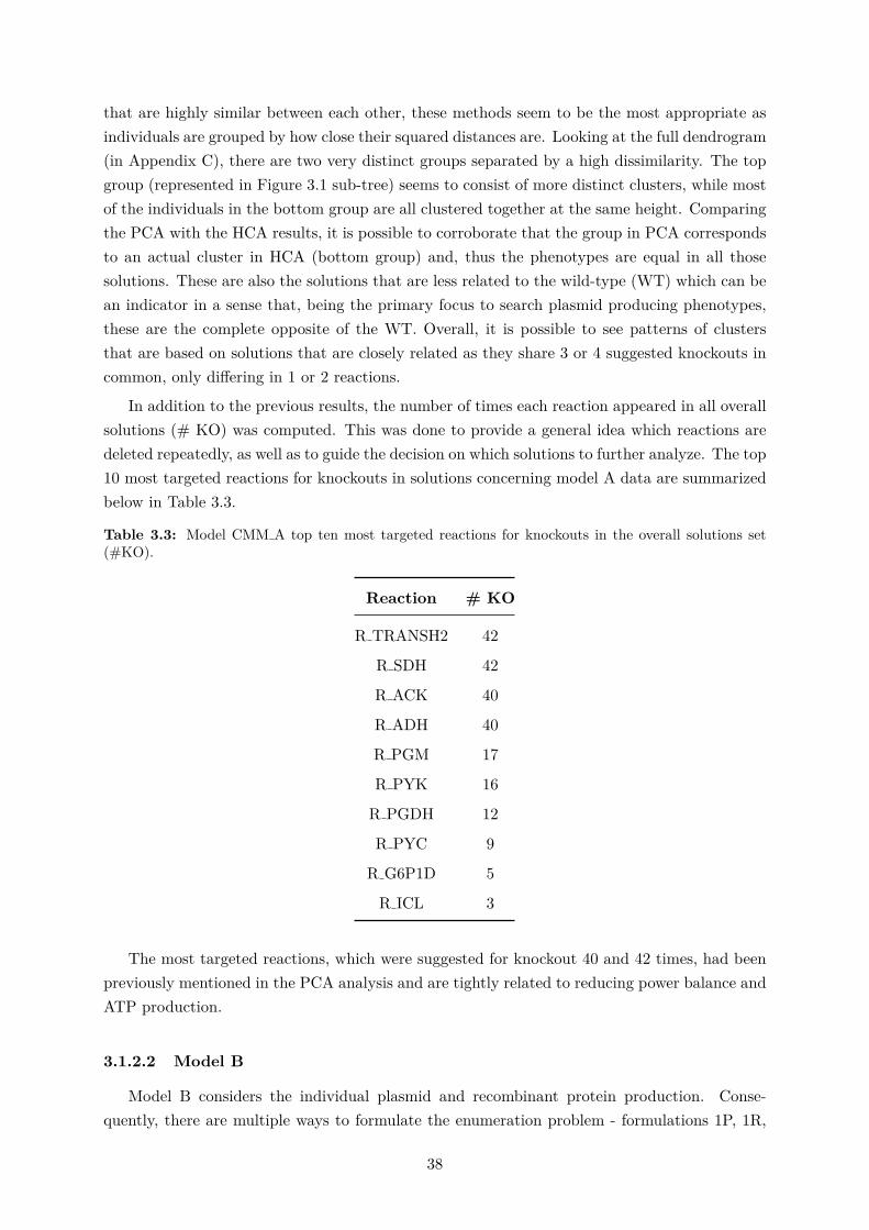
that are highly similar between each other, these methods seem to be the most appropriate asindividuals are grouped by how close their squared distances are. Looking at the full dendrogram(in Appendix C), there are two very distinct groups separated by a high dissimilarity. The topgroup (represented in Figure 3.1 sub-tree) seems to consist of more distinct clusters, while mostof the individuals in the bottom group are all clustered together at the same height. Comparingthe PCA with the HCA results, it is possible to corroborate that the group in PCA correspondsto an actual cluster in HCA (bottom group) and, thus the phenotypes are equal in all thosesolutions. These are also the solutions that are less related to the wild-type (WT) which can bean indicator in a sense that, being the primary focus to search plasmid producing phenotypes,these are the complete opposite of the WT. Overall, it is possible to see patterns of clustersthat are based on solutions that are closely related as they share 3 or 4 suggested knockouts incommon, only differing in 1 or 2 reactions.

In addition to the previous results, the number of times each reaction appeared in all overallsolutions (# KO) was computed. This was done to provide a general idea which reactions aredeleted repeatedly, as well as to guide the decision on which solutions to further analyze. The top10 most targeted reactions for knockouts in solutions concerning model A data are summarizedbelow in Table 3.3.

Table 3.3: Model CMM A top ten most targeted reactions for knockouts in the overall solutions set(#KO).

Reaction # KO

R TRANSH2 42

R SDH 42

R ACK 40

R ADH 40

R PGM 17

R PYK 16

R PGDH 12

R PYC 9

R G6P1D 5

R ICL 3

The most targeted reactions, which were suggested for knockout 40 and 42 times, had beenpreviously mentioned in the PCA analysis and are tightly related to reducing power balance andATP production.

3.1.2.2 Model B

Model B considers the individual plasmid and recombinant protein production. Conse-quently, there are multiple ways to formulate the enumeration problem - formulations 1P, 1R,

38

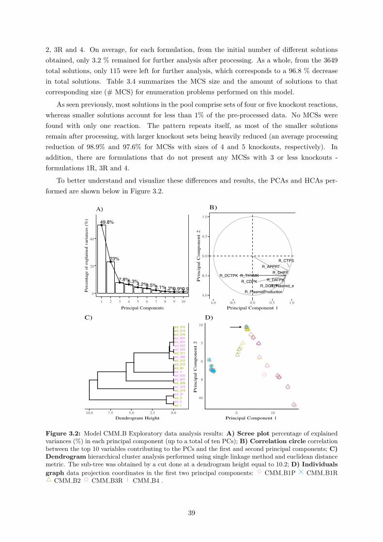
2, 3R and 4. On average, for each formulation, from the initial number of different solutionsobtained, only 3.2 % remained for further analysis after processing. As a whole, from the 3649total solutions, only 115 were left for further analysis, which corresponds to a 96.8 % decreasein total solutions. Table 3.4 summarizes the MCS size and the amount of solutions to thatcorresponding size (# MCS) for enumeration problems performed on this model.

As seen previously, most solutions in the pool comprise sets of four or five knockout reactions,whereas smaller solutions account for less than 1% of the pre-processed data. No MCSs werefound with only one reaction. The pattern repeats itself, as most of the smaller solutionsremain after processing, with larger knockout sets being heavily reduced (an average processingreduction of 98.9% and 97.6% for MCSs with sizes of 4 and 5 knockouts, respectively). Inaddition, there are formulations that do not present any MCSs with 3 or less knockouts -formulations 1R, 3R and 4.

To better understand and visualize these differences and results, the PCAs and HCAs per-formed are shown below in Figure 3.2.

●

●

●●

● ●●

● ● ●

49.8%

23%

7.8%6.3%4.2%3.5%2.1%1.2%0.9%0.9%0

20

40

1 2 3 4 5 6 7 8 9 10

Principal Components

Perce

ntage of

exp

lained

varia

nces

(%

)

A)

R_THYMKR_DHFR

R_CDPKR_DCTPK

R_DATPKR_DGTPKR_Plasmid_e

R_PlasmidProduction

R_APPRTR_CTPS

�1.0

�0.5

0.0

0.5

1.0

�1.0 �0.5 0.0 0.5 1.0Principal Component 1

Pri

nci

pal

Com

pon

ent

2

B)

sol_1sol_2sol_3sol_31sol_313sol_343sol_309sol_820sol_628sol_4sol_60sol_310sol_312sol_486sol_311sol_629sol_632sol_631sol_630sol_316sol_314sol_315

0.02.55.07.510.0 Dendrogram Height

C)

�10

�5

0

5

10

0 10Principal Component 1

Pri

nci

pal

Com

pon

ent

2

D)

Figure 3.2: Model CMM B Exploratory data analysis results: A) Scree plot percentage of explainedvariances (%) in each principal component (up to a total of ten PCs); B) Correlation circle correlationbetween the top 10 variables contributing to the PCs and the first and second principal components; C)Dendrogram hierarchical cluster analysis performed using single linkage method and euclidean distancemetric. The sub-tree was obtained by a cut done at a dendrogram height equal to 10.2; D) Individualsgraph data projection coordinates in the first two principal components: CMM B1P CMM B1R

CMM B2 CMM B3R CMM B4 .

39

Table 3.4: Model CMM B Summary of the suggested knockout number in a solution (MCS Size) andthe amount of solutions that have that size (# MCS), corresponding to each formulation before (pre-)and after (post-) processing steps.

Formulation MCS Size # MCS

Pre-Processing 1P

1 0 (0%)

2 3 (0.3%)

3 1 (0.1%)

4 186 (21.7%)

5 669 (77.9%)

Total 859

Pre-Processing 1R

1 0 (0%)

2 0 (0%)

3 0 (0%)

4 128 (20%)

5 501 (80%)

Total 629

Pre-Processing 2

1 0 (0%)

2 3 (0.3%)

3 1 (0.1%)

4 196 (21.7%)

5 703 (77.9%)

Total 903

Pre-Processing 3R

1 0 (0%)

2 0 (0%)

3 0 (0%)

4 128 (20%)

5 501 (80%)

Total 629

Pre-Processing 4

1 0 (0%)

2 0 (0%)

3 0 (0%)

4 128 (20%)

5 128 (20%)

Total 629

Formulation MCS Size # MCS

Post-Processing 1P

1 0 (0%)

2 1 (5%)

3 1 (5%)

4 2 (10%)

5 16 (80%)

Total 20

Post-Processing 1R

1 0 (0%)

2 0 (0%)

3 0 (0%)

4 2 (10%)

5 18 (90%)

Total 20

Post-Processing 2

1 0 (0%)

2 1 (2.8%)

3 1 (2.8%)

4 9 (25.7%)

5 24 (68.7%)

Total 35

Post-Processing 3R

1 0 (0%)

2 0 (0%)

3 0 (0%)

4 2 (10%)

5 18 (90%)

Total 20

Post-Processing 4

1 0 (0%)

2 0 (0%)

3 0 (0%)

4 2 (10%)

5 18 (90%)

Total 20

From the scree plot it is possible to compute that at least seven principal components arenecessary to explain approximately 97.0 % variance in these data. In comparison to the previousmodel, at least two more dimensions are required to achieve almost the same variance percentage,meaning that, by introducing the recombinant protein reaction in the model, more contrast anddivergence was included. Concerning model B data, two principal components were chosen tobe analyzed as they account for 72.8 % of cumulative explained variance percentage. Althoughthis value is 13.4 % lower than the previous model, it still considers a reasonable amount ofexplained variance in just two dimensions. This also corroborates that the IFNγ production

40

reaction introduced more variation in the system.

From the correlation circle, it is possible to visualize that all top ten contributing variablesshare the same amount of contribution to the components as their arrows present the same length(equal to the correlation circle radius, which is equal to one). Furthermore, all ten variables arein the negative side of component 2 and positive side of component 1 but are strongly positivelycorrelated with each other. Two interesting reactions that contribute to this variance are theones related to plasmid production (R PlasmidProduction and R Plasmid e). By adding therecombinant protein production reaction, it seems that producing a plasmid became extremelyvariable and perhaps dependant on precursors availability, now that the cell may require aminoacids for IFNγ production. The remaining reactions are mostly related to nucleotide synthesis.Four of these account for deoxyribonucleotide triphosphate (dNTPs) synthesis which are theprecursors for plasmid production (R DCTPK, R THYMK, R DGTPK and R DATPK thatcorrespond to the dCTP, dTTP, dGTP and dATP synthesis, respectively). The remaining vari-ables concern other precursors necessary for dNTP synthesis. The only outlier is R DHFR thatbelongs to the one carbon units family but, nevertheless, produces an important compound fornucleotide synthesis reactions (THF). Overall, by introducing the recombinant protein produc-tion, all top contributing variables are related with plasmid production and nucleotide synthesisand, thus it is expected that these reactions present a strong positive correlation.

As far as the individuals graph is concerned, this analysis shows that there is a clear sepa-ration between most solutions from formulations 1P and 2, in contrast to formulations 1R, 3Rand 4. In addition, a point in space is clearly seen that has all possible formulations overlapped(highlighted by the arrow in Figure 3.2). This point naturally corresponds to the WTs for eachformulation as it presents always the same phenotype. The data points that are completelyon top of each other suggest a very strong grouping of equal phenotypes. In fact, all the solu-tions for these three enumerations are exactly the same, meaning that they can be treated asone, having a total of 60 different solutions that can be reduced to 20 solutions that explainthe exact same phenotype. Most of these solutions identify a reaction that concerns to reducingpower (R TRANSH2 ) in addition to combinations of reactions from the pentose phosphate path-way (PPP) that are knocked out at different stages (R 6PGDH, R TALA1, R R5P1, R TKT1,R G1D and R GLUCK ). Moreover, regarding the other two formulations, some solutions maybe grouped but there is more variety in these formulations. In addition, a few of these solutionsare closely related to the WTs phenotype.

From the full HCA dendrogram (in Appendix C) it is possible to corroborate that there isa complete separation based on dissimilarity for the previously mentioned PCA groups. In thiscase it is harder to find an evident cut-off height that can be helpful to separate different clustersas there are plenty of options at many heights. Nevertheless, it is possible to at least isolate agroup as shown in Figure 3.2 sub-tree where a cut-off of 10.2 was applied. It is also available tosee which solutions are closer to the WT phenotype and which ones are not. Overall, this HCAis helpful to visualize the solutions group separation as well as understand that the inclusionof the recombinant protein added a level of variation in the system that is shown by the newmultiple ways to cluster all the solutions.

41

Moreover, the top ten targeted reactions for suggested knockouts in model B data solutionset are given below by Table 3.5.

Table 3.5: Model CMM B top ten most targeted reactions for knockouts in the overall solutions set(#KO).

Reaction # KO

R TRANSH2 77

R PGM 60

R 6PGDH 58

R PYK 38

R PGI 32

R PGDH 27

R G1D // R GLUCK 23

R R5PI // R TALA2 // R TKT1 22

R PFK 20

R PYC 19

Once more R TRANSH2 is the most suggested knockout in the solution set. Top KOs arereactions concerning glycolysis and gluconeogenesis. Furthermore, some also concern the PPPand the sole reaction representing the Entner Doudoroff (ED) pathway (R PGDH ) is present.In general, all these reactions belong to bacterial primary metabolism and to pathways whosegoal is to catabolize glucose to pyruvic acid.

3.1.2.3 Model C

Model C considers the individual plasmid, recombinant protein and resistance marker pro-duction, and thus there are multiple ways to formulate the enumeration problem- formulations1P, 1 R, 1M, 2, 3R, 3M and 4. On average, for each formulation, from the initial number ofdifferent solutions, only 2.5 % prevailed for further analysis in the post-processing steps. As awhole, from a total of 2770 solutions, only 76 remained for further analysis, which correspondsapproximately to a 97.3 % total solutions decrease. Table 3.6 summarizes the MCS size andthe amount of solutions correspondent to that size for all enumeration problems performed onmodel C.

42

Table 3.6: Model CMM C Summary of the suggested knockout number in a solution (MCS Size) andthe amount of solutions that have that size (# MCS), corresponding to each formulation before (pre-)and after (post-) processing steps.

Formulation MCS Size # MCS

Pre-Processing 1P

1 0 (0%)

2 3 (0.4%)

3 1 (0.1%)

4 186 (23.5%)

5 601(76%)

Total 791

Pre-Processing 1R

1 0 (0%)

2 0 (0%)

3 0 (0%)

4 2 (0.7%)

5 268 (99.3%)

Total 270

Pre-Processing 1M

1 0 (0%)

2 0 (0%)

3 0 (0%)

4 0 (0%)

5 319 (100%)

Total 319

Pre-Processing 2

1 0 (0%)

2 3 (0.5%)

3 1 (0.2%)

4 196 (34.3%)

5 371 (65%)

Total 571

Pre-Processing 3R

1 0 (0%)

2 0 (0%)

3 0 (0%)

4 2 (0,7%)

5 268 (99.3%)

Total 270

Pre-Processing 3M

1 0 (0%)

2 0 (0%)

3 0 (0%)

4 0 (0%)

5 319 (100%)

Total 319

Pre-Processing 4

1 0 (0%)

2 0 (0%)

3 0 (0%)

4 2 (0.9%)

5 228 (99.1%)

Total 230

Formulation MCS Size # MCS

Post-Processing 1P

1 0 (0%)

2 1 (5%)

3 1 (5%)

4 2 (10%)

5 15(80%)

Total 19

Post-Processing 1R

1 0 (0%)

2 0 (0%)

3 0 (0%)

4 2 (100%)

5 0 (0%)

Total 2

Post-Processing 1M

1 0 (0%)

2 0 (0%)

3 0 (0%)

4 0 (0%)

5 0 (0%)

Total 0

Post-Processing 2

1 0 (0%)

2 1 (3%)

3 1 (3%)

4 9 (25.7%)

5 24 (68.3%)

Total 35

Post-Processing 3R

1 0 (0%)

2 0 (0%)

3 0 (0%)

4 2 (100%)

5 0 (0%)

Total 2

Post-Processing 3M

1 0 (0%)

2 0 (0%)

3 0 (0%)

4 0 (0%)

5 0(0%)

Total 0

Post-Processing 4

1 0 (0%)

2 0 (0%)

3 0 (0%)

4 0 (0%)

5 18 (100%)

Total 18

43

Again, large solutions prevailed over smaller solutions (1, 2 and 3 knockouts), which accountfor about 1% or less of the pre-processed data. No MCSs with one reaction were identified.Larger knockout solutions were reduced with an average processing reduction of 99.0 % and97.5 % for MCSs with size of 4 and 5 deletions, respectively. Some formulations do not presentsolutions with 3 and 4 knockouts or below - formulations 1R, 1M, 3R,3M, 4. Interestingly,some formulations regarding resistance marker production did not survive the processing steps(formulations 1M and 3M). In addition, formulations for the recombinant protein lost 99.3 % oftheir solutions, where only 2 remained. Overall, with the resistance marker introduction fewersolutions were computed and got through the processing steps.

●

●

●

●●

● ● ● ● ●

46.8%

25.4%

9.3%6.5%5.3%

2.1%1.8%1.3%0.8%0.3%0

10

20

30

40

50

1 2 3 4 5 6 7 8 9 10Principal Components

Perce

ntag

e of e

xplai

ned

varia

nces

(%)

A)

R_GUAKR_I5MPDH

R_CTPS R_APPRT

R_UMPK R_ASPCMT

R_DHFRR_THYMK

R_CDPK R_DCTPK

−1.0

−0.5

0.0

0.5

1.0

−1.0 −0.5 0.0 0.5 1.0Principal Component 1

Pri

nci

pal

Com

pon

ent

2

B)

sol_2sol_11sol_3sol_31sol_220sol_677sol_217sol_1931sol_678sol_101sol_149sol_218sol_221sol_676sol_219sol_682sol_681sol_680sol_679sol_236sol_234sol_235

0.02.55.07.510.0 Dendrogram Height

C)

−5

0

5

−10 0 10Principal Component 1

Pri

nci

pal

Com

pon

ent

2

D)

Figure 3.3: Model CMM C Exploratory data analysis results: A) Scree plot percentage of explainedvariances (%) in each principal component (up to a total of ten PCs); B) Correlation circle correlationbetween the top 10 variables contributing to the PCs and the first and second principal components; C)Dendrogram hierarchical cluster analysis performed using single linkage method and euclidean distancemetric. The sub-tree was obtained by a cut done at a dendrogram height equal to 10; D) Individualsgraph data projection coordinates in the first two principal components: CMM C1P CMM C1R

CMM C2 CMM C3R CMM C4 .

The scree plot shows that a minimum of seven principal components are required to explainapproximately 97.2 % variance in this data, which is nearly equal to the previous model screeplot. Regarding this model data, two principal components were once more chosen to be analyzedand account for 72.2 % of cumulative explained variance, which is a reasonable amount of

44

explained variation in a two dimensional space. This value is similar to the previous one,which may be indicative that, by adding the resistance marker production reaction, there wasnot a major shift and introduction of divergence. This may happen as the resistance markeris essentially another protein to be produced and, thus, the amino acids required for the IFNγproduction are the same needed for the resistance marker production, but in different quantities.Comparing to model A, models B and C have a less gap difference as their core dissimilarity relieson one protein production reaction (and not plasmid, where nucleotides are involved instead ofamino acids).

Analyzing the correlation circle, it is possible to state that, again, all top ten variables equallycontribute to the components as they show equivalent arrow length. All these reactions are inthe positive side of the second principal component and the negative side of the first compo-nent, and demonstrate a strong positive correlation among each other. In comparison to theprevious model, it is interesting to note that, with the addition of the resistance marker produc-tion, the reactions regarding plasmid production are no longer on the top contributing variables.Nevertheless, nine out of ten variables belong to the nucleotide synthesis family. Two of theseare related with plasmid production precursors (R DCTPK and R THYMK that correspondto dCTP and dTTP synthesis, respectively) and the remaining are related to other precursorsnecessary for dNTP synthesis. The former being reactions with respect to nucleoside monophos-phate (R ASPCMT for UMP synthesis), nucleoside diphosphate (R GUAK and R UMPK forGDP and UDP synthesis, respectively) and nucleoside triphosphate (R CDPK and R CTPS forCTP synthesis). Again, the only outlier corresponds to R DHFR that belongs to the one carbonunits family but, nevertheless is important in nucleotide synthesis. Overall, the main differencesbetween this model and the previous rely on the plasmid production reactions. Regardless,on both models, nucleotidic synthesis reactions are heavily represented as the top contributingvariables to variance.

Concerning the individuals graph, a similar pattern to the one analyzed previously canbe observed, where there is a clear separation between formulations 1P and 2, in contrast toformulations 1R, 3R and 4. There is also a point in space that has many possible formulationsoverlapped and that corresponds to the WTs. All overlapping data points suggest a stronggrouping of equal phenotypes as usual, and may be confirmed through HCA. The few solutionsfrom formulations 1R and 3R are, in fact, equal to each other which means they can be treatedas unique solutions. A noticeable difference comparing to model B is that formulation 4 hasits own independent grouping. Nevertheless, these solutions demonstrate similar behaviour tomodel B solutions where most have a reaction that concerns reducing power (R TRANSH2 )with combinations of PPP reactions (R 6PGDH, R TALA1, R R5P1, R TKT1, R G1D andR GLUCK ) and glycolysis/gluconeogenesis reactions (R PGI, R PGM, R PFK and R ENO).Furthermore, regarding the remaining two formulations, there is less grouping and more solutionvariety and these are the solutions more closely related to the WTs.

From the full HCA dendrogram (in Appendix C) it is possible to corroborate the separationvisualized on the score plot. Once more, it is harder to find an evident cut-off height that canbe helpful to separate different clusters as there are plenty of options. Regardless, it is possibleto isolate four main groups as seen in the full dendrogram colour labelling. Overall, the addition

45

of the phosphotransferase production did not add too much variation in the system as before.The grouping is very closely related to Model B results and there are not many new options orsolutions from this metabolic model.

Lastly, the top ten contributing knockouts concerning the overall model C solutions is sum-marized below in Table 3.7.

Table 3.7: Model CMM C top ten most targeted reactions for knockouts in the overall solutions set(#KO).

Reaction # KO

R PGM 48

R TRANHS2 39

R PYK 38

R PGDH 27

R 6PGDH 22

R PYC 19

R PGI 18

R MTHFT // R SDH 16

R G1D // R G6P1D // R GLUCK //

R R5PI // R TALA2 // R TKT110

R ENO // R PFK 8

These statistics are very similar to the previous ones (from model B) with just some smallerdifferences regarding knockout order. Nevertheless, it is interesting to note that R TRANSH2is still on top of the list. Overall, practically all reactions belong to a pathway that metabolizesglucose to pyruvic acid, with the exception that R MTHFT and R SDH belong to the onecarbon unit and TCA cycle family, respectively.

3.1.2.4 Model D

In Model D, plasmid and resistance marker productions are dependent on plasmid availabilityand, thus only one formulation was computed (formulation 1R). A major difference in theenumeration problem for this model is that it was allowed a MCS size of 8 knockouts as therewere not many solutions for smaller sized MCSs. From the initial 29 different solutions obtainedfor this problem, only 27.6 % remained for further analysis after processing steps. Table 3.8summarizes the number of knockouts in a solution and the number of solutions that have thatsize.

46

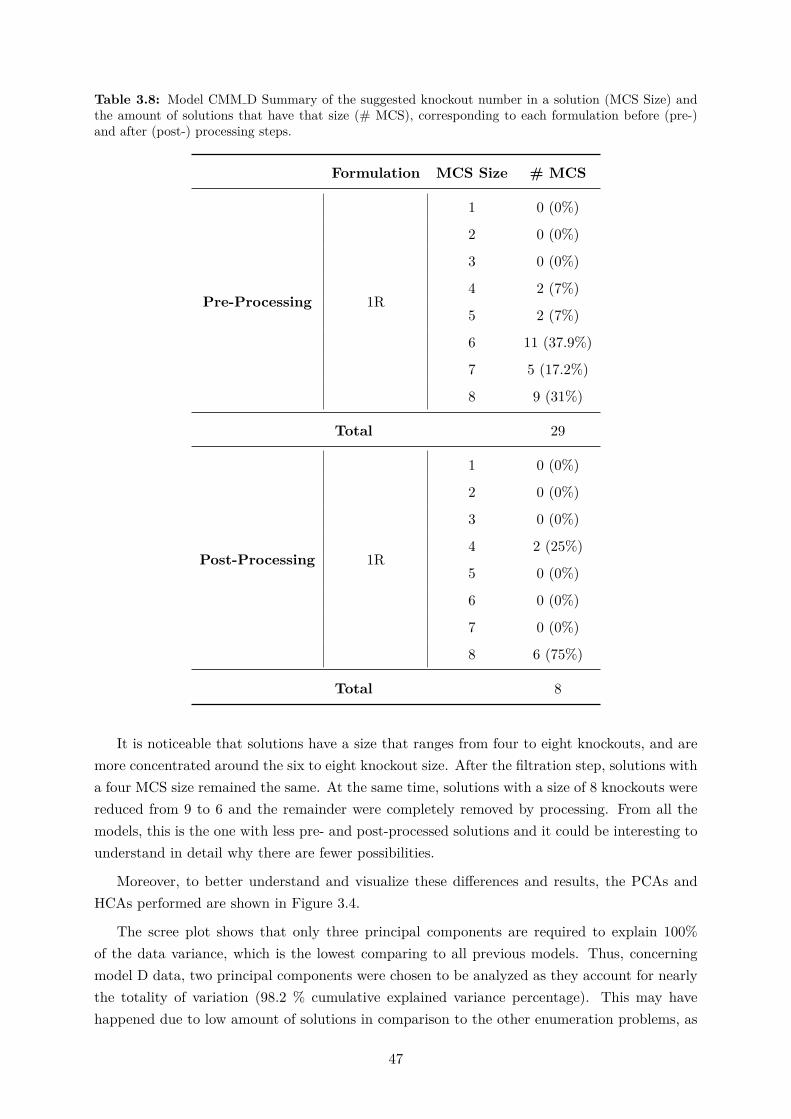
Table 3.8: Model CMM D Summary of the suggested knockout number in a solution (MCS Size) andthe amount of solutions that have that size (# MCS), corresponding to each formulation before (pre-)and after (post-) processing steps.

Formulation MCS Size # MCS

Pre-Processing 1R

1 0 (0%)

2 0 (0%)

3 0 (0%)

4 2 (7%)

5 2 (7%)

6 11 (37.9%)

7 5 (17.2%)

8 9 (31%)

Total 29

Post-Processing 1R

1 0 (0%)

2 0 (0%)

3 0 (0%)

4 2 (25%)

5 0 (0%)

6 0 (0%)

7 0 (0%)

8 6 (75%)

Total 8

It is noticeable that solutions have a size that ranges from four to eight knockouts, and aremore concentrated around the six to eight knockout size. After the filtration step, solutions witha four MCS size remained the same. At the same time, solutions with a size of 8 knockouts werereduced from 9 to 6 and the remainder were completely removed by processing. From all themodels, this is the one with less pre- and post-processed solutions and it could be interesting tounderstand in detail why there are fewer possibilities.

Moreover, to better understand and visualize these differences and results, the PCAs andHCAs performed are shown in Figure 3.4.

The scree plot shows that only three principal components are required to explain 100%of the data variance, which is the lowest comparing to all previous models. Thus, concerningmodel D data, two principal components were chosen to be analyzed as they account for nearlythe totality of variation (98.2 % cumulative explained variance percentage). This may havehappened due to low amount of solutions in comparison to the other enumeration problems, as

47

well as these solutions being possibly closely related regarding their variables (reaction fluxes)which will translate in low variation.

●

●

●● ● ● ● ●

60.1%

38.1%

1.8% 0% 0% 0% 0% 0%0

20

40

60

1 2 3 4 5 6 7 8Principal Components

Perce

ntag

e of e

xplai

ned

varia

nces

(%)

A)

R_ASPOX

R_HISDH

R_UMPK

R_ASPCMT

R_FAS4

R_ASPAS

R_FUM

R_CHORM

R_Protein_e

R_RecProduction

−1.0

−0.5

0.0

0.5

1.0

−1.0 −0.5 0.0 0.5 1.0Principal Component 1

Pri

nci

pal

Com

pon

ent

2

B)

WT

sol_0

sol_1

sol_22

sol_20

sol_21

sol_28

sol_26

sol_27

0510152025 Dendrogram Height

C)

−10

−5

0

5

−20 −15 −10 −5 0 5Principal Component 1

Pri

nci

pal

Com

pon

ent

2 D)

Figure 3.4: Model CMM D Exploratory data analysis results: A) Scree plot percentage of explainedvariances (%) in each principal component (up to a total of ten PCs); B) Correlation circle correlationbetween the top 10 variables contributing to the PCs and the first and second principal components; C)Dendrogram hierarchical cluster analysis performed using single linkage method and euclidean distancemetric. The sub-tree was obtained by a cut done at a dendrogram height equal to 15; D) Individualsgraph data projection coordinates in the first two principal components: CMM D1R.

Concerning the correlation circle, from all the models, this is the one that shows more di-versity. All top ten variables contribute equally to the components as previously stated andare separated in mainly three groups. The first group comprises R FAS4, R ASPCMT andR UMPK, which are reactions that are related to nucleotide synthesis. Furthermore, a secondgroup comprises the reactions R FUM, R CHORM, R ASPAS, R HISDH, R RecProduction andR Protein e. Contrarily to the previous group, these reactions are all related to amino acid syn-thesis, mainly histidine, aspartate and aromatic families. These two groups share a 180 degreewhich means that they are negatively correlated. In solutions, when amino acids are being pro-duced, it negatively influences nucleotide synthesis and vice-versa. This can be problematic sincein this model recombinant protein production is completely dependent on plasmid availability.The last group is composed only by R ASPOX which accounts for asparagine synthesis. Thisarrow is nearly orthogonal to the remaining vectors which implies that it does not have a strong

48

correlation to both groups. This result may be interesting as this reaction is tightly connectedwith R ASPAS and, therefore requires further flux analysis.

Furthermore, from the score plot and dendrogram it is possible to observe three distinctclusters. In sol 0 and sol 1 group, the MCS size is equal to 4 knock outs, where 3 arecontained in both solutions (R PEPCK, R TRANSH2, R PGI ) as the only difference lies onR GLUCK/R G1D. Moreover, for the middle and top clusters, the size increases to 8 knock-outs and these solutions share always six reactions in common (R 6PGDH, R PYK, R PGM,R MAL1, R MAL2 and R G6P1D) and the variation lies in PPP reactions R TALA2, R R5PIand R TKT1. The solutions from this model can be easily clustered for further analysis whichis an advantage in comparison to the previous models. However, eight knockout solutions maybe too much to apply in a biological setting and thus, lower knock out reactions that presentthe same phenotype may be prioritized. Regardless, in the next Section 3.1.3 the core criteriabehind which solutions are chosen for further detailed analysis will be described.

Lastly, since model D has fewer solutions, all the targeted reactions for knockouts concerningmodel D data are summarized below in Table 3.9.

Table 3.9: Model CMM D top most targeted reactions for knockouts in the overall solutions set (#KO).

Reaction # KO

R 6PGDH // R G6P1D // R MAL1 //

R MAL2 // R PGM // R PYK6

R PGI 5

R PFK 3

R PEPCK // R R5PI // R TALA2 //

R TKT1 // R TRANSH22

R G1D // R GLUCK 1

For model D targeted reactions, the pattern repeats itself where most reactions belong toglycolysis, ED or PPP. In this case, R TRANSH2 is not on top of list and the ’outliers’ fromthis group are R MAL1 and R MAL2 that correspond to malic enzymes from the TCA cycle.

3.1.3 Detailed Network Analysis

In order to understand and find solutions that could be possible candidates for testing invivo, a more detailed network analysis based on the pFBA fluxes was performed. For this, thefirst step was to identify two to three solutions that could be strong candidates based on whatwas explored in previous exploratory data analysis. The core idea is to compare the mutant fluxpattern to the WT and try to understand where is the carbon source being allocated and whatdifferences there are that seem relevant in a biological context. To find these solutions, a set ofselection criteria was applied as follows: (1) biomass growth reaction with a positive non-zeroflux; (2) priority to solutions with number of knockouts as low as possible; (3) avoid solutions

49

whose suggested knockouts are transport and exchange reactions; (4) priority to solutions thatare highly represented in the MCS pool; and (5) if possible, allow some variability regardingsuggested reactions pathways (for instance, a 2 KO solution with a reaction from fatty acidsynthesis and one from glycolysis). These sets of criteria were all applied, with no specific orderbut rather in a way that it is possible to make a weighted and conscious decision.

That being said, the first MCS analyzed comprises the reactions R PGI and R ENO (MCS1).This solution appears in enumeration problems CMM A1P, B1P, B2, C1P and C2. Moreover,this MCS follows most selection criteria and, in addition, is a good solution to compare to theprevious work done by Pandey et al. (2018) as it suggests pgi knockout. These simulationresults are presented in Figure 3.5, which displays a representation of the E. coli central carbonmetabolism.

In this solution, by knocking-out these two reactions in the model, it was possible to produceplasmid with a 4.36 BPCY, while keeping the growth rate at 34.1% of the parental strain. Inregard to the pgi knockout, since this reaction is a common node for different glucose catabolismpathways, its inactivation is particularly relevant for studying metabolic behaviour as carbonflux is redirected towards the PP pathway and/or the ED pathway. This flux rerouteing hasa profound impact in redox balance where transhydrogenases have a critical role (Canonacoet al., 2001). Moreover, concerning the eno knockout, this reaction is the penultimate step ofglycolysis and catalyzes the reversible reaction between 2-phospho-D-glycerate and PEP. It isalso a relevant reaction to study as it has an important role in gluconeogenesis. Regardingthe latter knockout, there is a lack of experimental 13C-fluxomics data, which can difficult thedouble knockout mutant flux distribution analysis (Long & Antoniewicz, 2014).

From the simulated flux distribution, it is possible to indicate that practically all glucoseflux is redirected to the ED pathway and that there is not reallocation towards the oxidative PPpathway. In previous 13C-MFA studies of a pgi-knockout strain it was experimentally determinedthat the PP pathway was the major route for glucose metabolism, providing a high NADPHsource. Nevertheless, the ED pathway was also actively catalyzing a minor fraction of glucose inboth wild-type and mutant strains (Hua et al.,2003; Fischer & Sauer, 2003). Although this singlepgi-knockout MFA experimental results do not match the predicted pFBA flux distributions, itis important to take into consideration that our simulations concern a double knockout. Thus,the eno-knockout may present an important role in flux redirection. It is possible that, in ourMCS simulation, a carbon flux allocation priority is shifted towards ED pathway as it is a moredirect way to obtain T3P readily available to subsequently produce, for instance, serine familyamino acids.

Moreover, in a study performed by Canonaco and Sauer it was shown that pgi inactivationled to a drastically reduction in maximum growth rate from 0.74 to 0.16 h-1. In this mutant,an accumulation of NADPH due to an insufficient re-oxidation was also observed. The deficitobserved in the growth rate was partly recovered by overexpressing the soluble transhydrogenaseUdhA. Since this enzyme is responsible for converting NADPH into NADH, there is a probabilitythat the growth recovery was due to the restored redox balance. In a cell, the redox balance ismainly described by the ratios between NAD+/NADH and NADP+/NADPH.

50

MCS1 - {R PGI; R ENO}

Figure 3.5: MCS1 metabolic flux distribution within central carbon metabolism of E. coli wild-type(top values) and ∆pgi∆eno double knockout mutant (bottom values). Fluxes are given relative to thespecific glucose consumption rate of 100 mmol/g · h and are expressed as the net fluxes. Knocked-outreactions are highlighted by a red cross and respective reaction name. Reactions from the mutant pFBAdistributions that did not present flux were highlighted with red. Arrows indicate the directions of theproposed metabolic model (negative fluxes correspond to the inverse reaction). For abbreviations anddetailed reactions, vide Appendix A.

51

These molecules participate in oxidation-reduction reactions and are specialized in carryinghigh-energy electrons and hydrogens, while transferring them to different sets of molecules.The main difference between these two molecules lies in NADH being mostly used in catabolicpathways and NADPH in anabolic pathways. Concerning catabolic reactions, NAD+ serves asan oxidizing agent and is reduced to NADH whereas, in anabolic reactions, NADPH serves asa reducing agent and provides high-energy electron being reduced to NADP+. The differenceof a single phosphate group has no effect in both molecules redox properties; however, it helpsenzymes distinguish these substrates. This is important so that both catabolic and anabolicpathways can be independently regulated, preventing futile metabolic cycles (Alberts et al.,2002; Berg et al., 2002). Considering Canonaco and Sauer experimental results, the fact that inour simulation the PP pathway is inactive can represent an advantage to the cell, since preventsexcessive NADPH accumulation and a potential redox unbalance. However, the cell still requiresa NADPH source to support anabolic metabolism.

When the PPP is inactive, NADPH production can potentially be achieved by three differentroutes in E. coli : (1) the NADPH dependent malic enzyme; (2) the membrane-bound tran-shydrogenase PntAB; and (3) the soluble transhydrogenase UdhA (Canonaco et al., 2001). Thefirst hypothesis is not feasible as our double-knockout pFBA flux distributions (in Figure 3.5)show that the reactions regarding malic enzymes are inactive (reaction R MAL1 and R MAL2 ).This is supported by experimental evidence that demonstrates that in pgi-knockout strains thereis no malic enzyme activity(Canonaco et al., 2001). Additionally, the behavior observed in thissingle knockout is expectable to be seen in the double mutant. Concerning options 2 and 3, inour metabolic network, these re-oxidation mechanisms are represented as two distinct reactions(R TRANSH1 and R TRANSH2 ). From our results, it is possible to see that the flux towardsR TRANSH1, which generates NADPH from NADH, is one of the highest. In fact, this tran-shydrogenase activation is our main NADPH source as it accounts for 78% of total NADPHpool. The remaining 22% are solely allocated from 5,10-methenyltetrahydrofolate (MeTHF)production reaction (R MTHFD), since there is no carbon flux directed towards the oxidativebranch of PP pathway.

Since in the flux distribution of the pgi and eno double knockout mutant, the NADPHavailability is dependent on NADH pool, it is important to understand its source. In oursimulation, NADH accumulation is mostly originated via TCA cycle (31.7 %) and via glycolyticpathway (30.5 %). Comparing with the WT simulation, an increment in the TCA cycle fluxis observed which can explain NADH availability in the mutant. In particular, the flux in theconversion of malate into oxaloacetate is increased by 15-fold, providing a good NADH source.Contrarily to what was observed in the simulations with the WT strain, the glyoxylate shunt fluxwas activated in this double mutant. This is corroborated by some findings in a study performedby Usui et al. . The authors reported a sequential increment in the flux through the glyoxylateshunt as the phosphoglucose isomerase was successively down-expressed until it was completelyknocked-out. It is known that in E. coli, the glyoxylate shunt is utilized mainly for the supplyof oxaloacetate to the TCA cycle via malate by using isocitrate and acetyl-CoA (Kondrashovet al., 2006). Thus, the activation of the glyoxylate shunt in the mutant strain increases malateavailability, which in its turn is converted to oxaloacetate releasing NADH. That being said,

52

probably in this simulation, the glyoxylate shunt activation is essential to provide: (1) extraNADH to fulfill the NADPH requirements of the cell; and (2) oxaloacetate, that is an importantprecursor to a large family of amino acids, some of which are required in the nucleotide synthesis(such as L-aspartate).

This solution was generated in the model that only contemplates plasmid production, thus itis important to understand the flux allocation into nucleotide synthesis. The metabolite ribose5-phosphate (R5P) of the PP pathway is the common building block in the de novo purine andpyrimidine synthesis pathways (Moffatt & Ashihara, 2003). In our simulation, this metabolite isgenerated by a reverse path through the non-oxidative PP pathway branch starting from the T3Pgenerated in the ED pathway. From R5P, the flux is then directed towards PRPP, a commonprecursor to nucleotide synthesis (Moffatt & Ashihara, 2003). In the pFBA simulation resultsfrom the mutant, the flux increases in the previously described reactions with a consequent in-crement in nucleotide synthesis. Comparing with the WT flux values, there is an average 27-foldincrease in the flux towards dNTPs synthesis reactions. In addition to nucleotide synthesis, en-ergy expenditure concerning nucleotidic bonding needs to be taken into consideration (Equation2.1). This means that, in our simulations, the flux of ATP must match this nucleotide synthesisincrement to lead to a higher plasmid production. From the double mutant knockout pFBAresults, it is possible to conclude that the TCA cycle operates predominantly for ATP generationby producing NADH that goes through oxidative phosphorylation. This is corroborated by themodel reactions regarding oxidative phosphorylation (R ATPS1 and R ATPS2 that are NADHand FADH2 dependent, respectively) accounting for approximately 88.1% of ATP generationflux. In particular, it is interesting to note that in the WT, FADH2 production via TCA cycleis non-existent, whereas in the mutant it becomes an important energy source. Additionally, inthe double knockout mutant, since the glycolytic pathway is mostly inactive, it provides only11.4% of the energy source to the system.

Overall, this MCS is helpful in corroborating the findings by Pandey et al. even if theflux distribution does not fully match the experimental results. Nevertheless, it is necessaryto take into consideration that our results are based on pgi and eno knockouts, instead ofsingle knockout mutants. In spite of that, our double mutant did improve in silico plasmidproduction. However, it would be interesting to compare this simulation with experimentaldata from 13C-MFA of single eno-knockout strains as well as double pgi and eno knockoutstrains to confirm, for instance, if the flux is preferably allocated towards ED pathway and howit impacts NADH/NADPH pool availability. In addition, contingent on the results from thesingle and/or double knockouts, it could be interesting to study the soluble transhydrogenaseUdhA expression with the purpose to verify and corroborate its kinetic limitations in cell growth,plasmid and/or recombinant protein production.

Moreover, a second MCS was analyzed in detail that comprises reactions R PGM, R G6P1D,R PYK and R PYC. This solution appears in enumeration problems CMM B1P, B2, C1P andC2. Moreover, this MCS matches most selection criteria and, from all the solutions in all models,is the one that presents the highest BPCY (regarding plasmid production). Additionally, thesuggested knockouts show a reasonable variability regarding their role in the metabolism. Thesesimulation results are presented in Figure 3.6.

53

MCS2 - {R PGM; R G6P1D; R PYK; R PYC}

Figure 3.6: MCS2 metabolic flux distribution within central carbon metabolism of E. coli wild-type(top values) and ∆pgm/agp∆pykA/pykF∆zwf∆ppc quadruple knockout mutant (bottom values). Fluxesare given relative to the specific glucose consumption rate of 100 mmol/g · h and are expressed as thenet fluxes. Knocked-out reactions are highlighted by a red cross and respective reaction name. Reactionsfrom the mutant pFBA distributions that did not show flux were highlighted with red. Arrows indicatethe directions of the proposed metabolic model (negative fluxes correspond to the inverse reaction). Forabbreviations and detailed reactions, vide Appendix A.

54

In this solution, by knocking-out these four reactions in the model, it was possible to produceplasmid with a 5.23 BPCY, while keeping the growth rate at 49.8% of the WT strain. However,there was no flux going through the recombinant protein and resistance marker productionreactions. In these models (B and C), the plasmid, resistance marker and recombinant proteinsynthesis share common precursors. Thus, by optimizing the flux through one of these products,the increasing required pool of precursors will limit the synthesis of the remaining reactions. Forthis reason, it is rather difficult to obtain solutions where production of 2 or 3 of these productstake place at the same time.

The inactivated reactions from this MCS comprise two reactions from glycolysis and gluco-neogenesis, namely R PGM and R PYK that are encoded by genes pgm/agp and pykA/pykF,respectively. In addition, R G6P1D is the first step in the oxidative PP pathway, catalyzed bythe enzyme glucose-6-phosphate 1-dehydrogenase that is encoded by gene zwf, and R PYC thatis an anaplerotic reaction whose catalytic enzyme is encoded by the ppc gene.

Accordingly to the flux distribution shown in Figure 3.6, the pgm/agp and zwf inactivation,led to a rewire of the flux towards glycolysis in comparison to the previous simulation results.Additionally, the oxidative PP Pathway and ED pathway had no flux. In 13C-MFA studiesof zwf -knockout strains, it was revealed that the disruption of glucose 6-phosphate dehydro-genase was counteracted by local rerouting via the glycolysis. Additionally, the authors haveshown that the mutant strain synthesized the PPP-derived compounds independently from theoxidative branch by directing the carbon flow from glycolysis into the reversed non-oxidativePPP branch. Thus, it indicates that the glycolytic metabolites triose 3-phosphate and fructose-6-phosphate compensated the lack of E4P and R5P (Hua et al., 2003; Nicolas et al., 2007).Regarding pgm/agp-knockout, there is a lack of biological fluxomics data, which can difficult theinterpretation of their role and behavior in our quadruple-knockout mutant.

Considering the data retrieved from the literature, the redirection of all carbon flux towardsglycolysis, avoiding the oxidative PP pathway, can result in a NADPH shortage - an essen-tial cofactor for anabolic metabolism (Nicolas et al., 2007). Thus, the zwf -knockout strainsmust have a coping mechanism tightly related to transhydrogenases and NADP(+)-dependentenzymes. Zhao et al., concluded that, as a response to this unbalance, the cell would useNADP(+)-dependent isocitrate dehydrogenase. This enzyme catalyzes the conversion of isoci-trate into 2-oxoglutarate while producing the majority of NADPH. However, the action of thissingle enzyme is not sufficient to fulfil the NADPH cellular requirements, thus activating otherenzymes such as transhydrogenases and NADP(+)-dependent malic enzyme is required. In ourmetabolic model, the reaction catalyzed by NADP(+)-dependent isocitrate dehydrogenase isnot represented, which may explain some discrepancies observed between experimental dataand simulation results. Similarly to what was observed in the MCS1 simulation, the source ofNADPH is a consequence of the flux going through R TRANSH1, that is responsible in convert-ing NADH to NADPH. In fact, this transhydrogenase activation is responsible for approximately82.5% of NADPH pool, while the remaining percentage is due to 5,10-methenyltetrahydrofolateproduction reaction (R MTHFD). Additionally, it was observed that the reactions catalyzed bythe malic enzymes have no flux. These enzymes catalyze NADH and NADPH production byconverting malate into pyruvate. In our simulation results, there is a high pyruvate accumula-

55

tion, derived from the PTS system (R PTS). This system is a distinct method used by bacteriafor sugar (namely glucose) uptake where the source of energy comes from PEP. For each moleculeof glucose that enters the cell, a molecule of pyruvate is produced. Thus, it is expected that it isnot necessary to overproduce pyruvate by using the malic enzymes. Instead, in our simulation,malate is converted into oxaloacetate releasing NADH that is later converted into NADPH bytranshydrogenases (R TRANSH1 ). Nevertheless, despite our results not showing evidence ofmalic enzyme activity, experimental evidence demonstrates that zwf -knockout strains allocated3% of their total carbon flux towards malic enzyme pathway (Zhao et al., 2004).

Moreover, focusing on pykA and pykF mutants, a study by Fischer and Sauer shows thatthe metabolic bypass of pyruvate kinase knockout is done via PEP carboxylase (ppc) and malicenzyme as the mutants exhibit lower fractions of oxaloacetate originated through the TCA cycleand higher fractions of pyruvate originated from malate. In addition to the R PYC anapleroticreaction, it was demonstrated a depletion of Pfk (R PFK ) by the accumulated PEP. Eventhough these genes are knocked out, PEP can still be converted to pyruvate through PTSand, in the pyk mutants, the ATP level from aerobic respiration is not significantly affected invivo (Zhu & Shimizu, 2005). Another important finding concerns excess NADPH produced bythe pyk-knockouts mutants, which is similar to pgi-knockouts strains that tend to overproduceNADPH and convert the excess NADPH into NADH using transhydrogenases (Toya et al., 2010).However, in both simulation and experimental data, the zwf mutant activates the reversednon-oxidative PP pathway and no flux passes through the oxidative portion, thereby avoidingNADPH accumulation.

Furthermore, it was previously mentioned that pykA and pykF mutants would increase PEPcarboxylase (R PYC ) activity as it was a metabolic bypass for PEP metabolism. However, inour MCS solution, this enzyme is also inactivated so it is important to understand the effectson the metabolism. Evidences from a study done by Fong et al. reveal that, in ppc mutants,the normally repressed glyoxylate replaced the anaplerotic function of PEP carboxylase. Eventhough, in different studies regarding single knockouts of zwf and pyk mutants, the glyoxylatepathway is inactive and negligible, in the simulation results from MCS2 this reaction is activated.This may be due to PEP carboxylase anaplerotic role substitution, as well as additional NADHproduction that may be converted to NADPH via transhydrogenases. This mechanism is similarwith what is previously observed in MCS1 solution, where NADH pool is originated from theTCA cycle, representing a flux increment between 3 and 13-fold in the reactions constitutingthis cycle when compared with the WT results. In particular, the flux of the conversion frommalate to oxaloacetate suffered a 13-fold increment, due to glyoxylate shunt activation, whichincreased the malate pool. Additionally, oxaloacetate is an amino acids precursor and is tightlyinvolved in nucleotide synthesis and consequent plasmid accumulation. Thus, this bypass is alsoimportant as it is the only source to indirectly produce oxaloacetate in our metabolic model.

Regarding nucleotide synthesis, it was observed a similar behavior to the previous resultsfrom MCS1. The flux starts from T3P and F6P and goes through the non-oxidative PP pathwayuntil R5P is formed, which is then converted to PRPP (a common precursor to the nucleotidesynthesis). Comparing to the WT pFBA results, it is possible to conclude that the flux towardsdNTPS synthesis reactions is increased 22 to 23-fold. Considering Equation 2.1, to concomitantly

56

increase the production of plasmid, an increment in the ATP pool is also required. Similarly,from these results it is possible to conclude that the TCA cycle operates predominantly forATP generation by producing NADH that goes through oxidative phosphorylation. This is cor-roborated by the model reactions regarding oxidative phosphorylation R ATPS1 and R ATPS2accounting for approximately 66.3 % of ATP generation. In particular, comparing the mutantto the WT, FADH2 production plays a relevant role in energy source as its reaction net flux in-creases from 0.0 to 34.4. Nevertheless, it is important to note that, in comparison to MCS1, thissimulation shows that one third of the ATP is also generated from glycolysis, as this pathwayis not blocked.

In summary, in this quadruple-knockout the main goal seems to be to redirect flux as muchas possible from G6P onwards and towards the glycolytic pathway. It is a solution that presentssimilar pFBA results to the previous one, however it has its differences. Namely, the carbonflux blockage towards the oxidative PP pathway (induced by the zwf deletion) that preventsNADPH overproduction, which is proven to be a limiting step towards growth and productionin other mutants, such as single pgi-knockout strains. Additionally, these simulation resultsmay be useful to explain some biological phenomena such as the glyoxylate shunt activation byanalyzing the ppc and pyk mutants synergy. Overall, it would be interesting to possibly combinesome of the findings from this MCS with the previous results, in order to construct a biologicalrelevant and well supported MCS. In addition, having more biological data on more than singleknockouts would be also useful to understand the metabolism and how the carbon flux is shifted.

Furthermore, a third and final MCS was analyzed in detail and comprises reactions R PEPCK,R TRANSH2, R PGI and R GLUCK. This solution appears in enumeration problems CMM B1R,B3R, B4, C1R and C3. Moreover, this MCS matches most selection criteria. Contrarily to theprevious MCS1 and MCS2, this solution has flux going through recombinant protein productionreaction, instead of plasmid production. Additionally, the suggested knockouts show a reason-able variability regarding their role in the metabolism. These simulations results are presentedin Figure 3.7 in an E. coli central carbon metabolism representation.

In this solution, by knocking-out these four reactions in the model, it was possible to pro-duce IFNγ with a 1.30 BPCY, while keeping the growth rate at a 14.6% of the parental strain.However, there was no flux going through the plasmid and phosphotransferase production reac-tions. This is due to the fact that this solution was originated from a formulation problem thatconsiders recombinant protein production optimization. Hence, it is rather difficult to obtainsolutions where production of 2 or 3 of these products take place at the same time.

The inactivated reactions from this solution comprise a reaction from glycolysis R PGI that isencoded by pgi gene; a reaction concerning an anaplerotic pathway (R PEPCK ) that is encodedby pck gene; a step in gluconate metabolism catalyzed by the enzyme gluconokinase (R GLUCK )that is encoded by genes idnK or gntK ; and a reaction regarding NADH regenerating throughNADPH (R TRANSH2 ), that is catalyzed by a transhydrogenase which is encoded by pntABor udhA genes.

57

MCS3 - {R PEPCK; R TRANSH2; R PGI; R GLUCK}

Figure 3.7: MCS3 metabolic flux distribution within central carbon metabolism of E. coli wild-type (topvalues) and ∆pck∆pgi∆pntAB/udhA∆idnK/gntK quadruple knockout mutant (bottom values). Fluxesare given relative to the specific glucose consumption rate of 100 mmol/g · h and are expressed as thenet fluxes. Knocked-out reactions are highlighted by a red cross and respective reaction name. Reactionsfrom the mutant pFBA distributions that did not show flux were highlighted with red. Arrows indicatethe directions of the proposed metabolic model (negative fluxes correspond to the inverse reaction). Forabbreviations and detailed reactions, vide Appendix A.

58

According to the flux distributions in Figure 3.7, the pgi and idnK/gntK inactivation led to arewire of the carbon flux towards the ED and PP pathways. Considering these pathways, therewas a 74.8% carbon allocation towards oxidative branch of PP pathway, while the remaining fluxwas redirected towards ED pathway. These predicted pFBA flux distributions are in accordancewith previous 13C-MFA studies of a pgi-knockout strain, where it was experimentally validatedthat the PP pathway was the major route for glucose metabolism after knocking-out pgi gene. Inaddition, these experimental studies proved that the ED pathway was also actively catalyzing aminor glucose fraction (Fischer & Sauer, 2003). Regarding idnK/gntK -knockout, there is a lackof biological fluxomics data, which can difficult the interpretation of its role in our quadruple-knockout mutant. Nevertheless, in our simulation results, it seems that this knockout mostlyreinforces the carbon flux redirection towards PP and ED pathways.

Considering our quadruple-knockout mutant pFBA flux distributions, there is a high NADPHproduction due to a flux allocation towards the PP pathway. Nearly 97.8% of NADPH isproduced in this pathway, while the remaining 2.2% are from 5,10-methenyltetrahydrofolate(MeTHF) production reaction (R MTHFD). NADPH is an important cofactor for anabolic re-actions. To increase recombinant protein production, a concomitant increment in amino acidspool is also required. Consequently, to produce these amino acids, a higher NADPH pool isnecessary. In our simulations, the conversion of NADPH into NADH, catalyzed by reactionR TRANSH2, is knocked out. This way, all NADPH generated through the PP pathway can beallocated towards biosynthetic pathways (such as amino acids precursors synthesis). However,experimental data retrieved from literature shows that carbon flux redirection to PP pathwayleads to an accumulation of NADPH due to an insufficient re-oxidation (Canonaco et al., 2001).This accumulation led to a reduction in growth rate that was later partly recovered by overex-pressing the soluble transhydrogenase UdhA. This enzyme is responsible for converting NADPHinto NADH, hence there is a probability that growth recovery was due to the restored redoxbalance, as previously described in MCS1. In our metabolic model, this mechanism is inacti-vated (R TRANSH2 ) and thus, our model is unable to re-oxidize NADPH through this reactionthat is catalyzed by transhydrogenase. Therefore, our simulation results may not correspondto a feasible biological state. Since pgi-knockouts were experimentally proven to accumulateNADPH, it is probable that a double pntAB/udhA and pgi-knockout is not able to strive ingrowth. Nevertheless, according to the amino acid synthesis requirements (Appendix B), andsince we want to improve plasmid and recombinant protein production, it is understandablethat the suggested knockouts try to increase cofactors pool such as NADPH. Hence, this so-lution could be a suggestion to test in vivo, as accumulated NADPH could be induced andredirected towards biosynthetic pathways.

Furthermore, in our simulation results, the flux is then directed towards the bottom half partof glycolysis and towards the TCA cycle. It is important to note in Figure 3.7 that the reactioninterconverting F6P and T3P shows a higher amount of net flux in comparison to the remainingreactions. This is due to a futile cycle in this interconversion. It can be considered that the realflux is given by the subtraction of fluxes and, thus this reaction is preferably going in the forwarddirection. Entering an interrupted TCA cycle, in comparison to the WT, there is an incrementon flux towards alpha-ketoglutarate formation (aKG) that is completely rewired towards glu-

59

tamic acid amino acids family production with no further conversion into SucCoa. Additionally,this increment towards aKG is accompanied by glyoxylate shunt activation. This activationleads to a flux re-allocation towards malate and succinate leading to a higher accumulationof oxaloacetate that is a precursor to aspartic acid amino acids family. Hence, both of thesemechanisms are essential to accumulate important biosynthetic precursors towards recombinantprotein production. This is also corroborated by the PEP carboxykinase knockout (R PEPCK )as it prevents oxaloacetate decarboxylation into PEP, increasing even more its availability tothe synthesis of these precursors. The results from an experimental study performed by Yanget al., (2003), proved that pck-inactivation led to glyoxylate shunt activation to participate inanaplerosis and replenish the TCA cycle. Hence, the experimental results from the literaturesupport the flux distributions obtained in our simulations.

Regarding IFNγ synthesis, most of the fluxes directed towards amino acids synthesis are in-creased when comparing with the WT simulation results. Comparing with the WT flux values,there is an average 1.5 to 2-fold increase through many amino acid synthesis reactions. Thesereactions are related to amino acids whose demand differs a lot from biomass to recombinantprotein production. Some examples of these amino acids are lysine, serine, phenylalanine, histi-dine and leucine. In addition to amino acids synthesis, energy expenditure concerning peptidicbonding needs to be considered. This means that, in our simulation, the flux of ATP mustfollow this amino acid synthesis increment to effectively lead to a higher recombinant proteinproduction. From the quadruple mutant knockout simulation results, it is possible to concludethat ATP generation is predominantly provided by oxidative phosphorylation as it accounts for74.2% of the energy source (reactions R ATPS1 and R ATPS2 that are NADH and FADH2

dependent, respectively). The NADH required for aerobic respiration is mostly provided byglycolysis (64.5%), while some is produced from the TCA cycle (27.0%). Moreover, FADH2

production is exclusively a result of succinate dehydrogenase activity in the TCA cycle.

Overall, in this quadruple-knockout the flux is redirected towards PP pathway with conse-quent NADPH accumulation due to transhydrogenase inactivation. Additionally, in comparisonto the WT simulation results, the higher flux through TCA cycle increases the amino acidssynthesis precursors such as oxaloacetate and alpha-ketoglutarate. From experimental data inthe literature, the in vivo application of these results probably will affect the maximum growthbut enhance plasmid and recombinant protein production.

3.2 Genome-scale Model

The GSM used to generate results was iJO136, whose reconstruction was done by Orth etal., 2011. The updated version of this model comprises 1367 associated genes, 2585 metabolicreactions and 1805 metabolites. In comparison to the CMM model, these metabolites andreactions can be compartmentalized, which is translated in another level of complexity and newtype of reactions, such as transport reactions.

60

3.2.1 Data Processing

All data were attempted to be generated for each formulation problem as previously describedin Chapter 2. However, formulations 2 and 4 will not be included in the GSM results as therewere not enough computational resources to generate them. A maximum knockout size of 6 wasallowed for each problem and all the solutions were stored as sets of strings encoding reactions.Equal to the CMM data generation, for each solution a pFBA flux distribution was computedand stored in a matrix.

Before analysing the data, a pre-processing step was performed to help reduce the number ofsolutions. In this case, a less broaden solution removal criterion was applied as the computationalrelevance was taken more into consideration than the biological one. Primarily, all solutionsthat were found and that were incompatible with the previously defined cellular constraintswere automatically removed. In conjunction with this, solutions whose production occurred ina mandatory way coupled to 99 % of biomass were kept. Essentially, it was verified if all cellularconstraints were followed and if the minimum product flux, with biomass growth fixed at 99%of its maximum value, was greater than zero.

For each model and formulation these filtration steps were applied. After processing, eachformulation data corresponding to a model was concatenated and analysed simultaneously. In-terestingly, it is important to note that model A (regarding plasmid production only) and modelD (a more complex model correlating all entities) did not have any solutions that remainedafter this processing step and, thus will not be mentioned in the following and further dataanalysis. As this genome-scale network comprises more reactions and alternative pathways thatmay result in different ways to metabolize glucose, possible explanations lie on flux allocation.For instance, a possible hypothesis is that the GSM has a high number of pathway alternativesto nucleotide metabolism and is not able to make it essential in order to produce the plasmid,unless a considerable amount of knockouts are introduced. Another possibility relies on energyand the possible fact that the cell is not able to produce enough ATP to be used in the nucleotidesynthesis pathway.

3.2.2 Exploratory Data Analysis

3.2.2.1 Model B

For model B possible enumeration problems, all formulations presented results. However,the solutions regarding plasmid production formulation (1P) did not survive the filtration step.On one hand, regarding 1R formulation, from an initial 1503 solutions, 195 remained for furtheranalysis which corresponds approximately to 13% of the initial pool. On the other hand, for 3Rformulation, from an initial higher solution number of 34 739, only 17 remained, correspondingto 0.049% of the initial pool, which makes it an extremely diluted solution pool comparing tothe previous formulation. Overall, accounting for all formulations, from a total of 37501 initialsolutions, only 0.57% (212) made it through the filtration process, which may be beneficial forfurther analysis. Table 3.10 summarizes the total number of solutions in each formulation forall enumeration problems performed on model B data.

61

Table 3.10: Model GSM B Summary of the total number of solutions gathered (#Solutions), corre-sponding to each formulation before (pre-) and after (post-) processing steps.

Formulation #Solutions

Pre-Processing1P

1 259

Post-Processing 0

Pre-Processing1R

1 503

Post-Processing 195

Pre-Processing3R

34 739

Post-Processing 17

From the post-processed set of 212 solutions there were a total of 15, 18 and 179 MCSs witha size of 4,5 and 6 suggested knockouts, respectively. Moreover, PCA and HCA were performedand the computed results for this set of solutions are shown below in Figure 3.8.

●

●

●

● ● ● ● ● ● ●

60.5%

15.1%

5.5%3% 2.2%1.6%1.4%1.3%1.1%0.9%

0

20

40

60

1 2 3 4 5 6 7 8 9 10Principal Components

Perce

ntag

e of e

xplai

ned

varia

nces

(%)

A)

R_METAT

R_GLUPRT

R_NADK

R_GTPCIR_DNTPPA

R_DHNPA2rR_DNMPPA

R_HPPK2 R_DHPS2

R_DHFS

−1.0

−0.5

0.0

0.5

1.0

−1.0 −0.5 0.0 0.5 1.0Principal Component 1

Pri

nci

pal

Com

pon

ent

2

B)

sol_9

sol_14

sol_13

sol_10

sol_11

sol_12

010203040 Dendrogram Height

C)

−20

−10

0

10

0 25 50 75Principal Component 1

Pri

nci

pal

Com

pon

ent

2

D)

Figure 3.8: Model GSM B Exploratory data analysis results: A) Scree plot percentage of explainedvariances (%) in each principal component (up to a total of ten PCs); B) Correlation circle correlationbetween the top 10 variables contributing to the PCs and the first and second principal components; C)Dendrogram hierarchical cluster analysis performed using single linkage method and euclidean distancemetric. The sub-tree was obtained by a cut done at a dendrogram height equal to 50; D) Individualsgraph data projection coordinates in the first two principal components: GSM B3R GSM B1R .

62

From the scree plot is it possible to conclude that ten principal components are requiredto explain 92.6 % variance in these data, which is a lower percentage and higher dimensionsrequired comparing to all previous CMM models. Nevertheless, if two principal components arechosen to represent the data, these account for 75.6 % of cumulative explained variance whichis a reasonable amount of variation in two dimensions and is comparable to previous models.Therefore, concerning model B data, this was the amount of principal components chosen forfurther PCA analysis.

Moving to the correlation circle, it is possible to visualize that all top ten contributingvariables share the same amount of contribution as their arrows share equal length. All tenvariables are in the positive side of the first principal component and negative side of principalcomponent 2, and demonstrate a strong positive correlation between each other. Moreover,seven out of ten variables correspond to reactions that belong to folate biosynthesis pathway(R DHFS, R DHPS2, R DNTPPA, R DHNPA2, R HPPK2, R GTPCI and R DNMPPA) atdifferent stages. Most of these reactions intervene in the synthesis of tetrahydrofolate, which isa cofactor in many reactions regarding, especially, de novo synthesis of purine and pyrimidinenucleotides and some amino acids interconversion, such as serine to glycine. The remainderreactions concern a NAD+ kinase (R NADK ), which accounts for NAD+ phosphorylation intoNADP+, which is an essential coenzyme that is reduced to NADPH primarily by the PP pathwayto provide reducing power in biosynthetic processes such as fatty acid biosynthesis and nucleotidesynthesis; a reaction regarding the conversion of PRPP into 5-phosphoribosyl-1-amine (PRA)using the ammonia group from the glutamine chain (R GLUPRT ) that is the committing step inde novo purine nucleotide synthesis; and S-adenosylmethionine synthesis reaction (R METAT )that is an important methyl and propylamino donor in polyamine biosynthesis. Overall, thetop contributing variables are concerning nucleotidic synthesis as previously described for thecorrelation plots from CMM models, with the difference that in this case, most of the reactionsintervene in reducing power balance and folate synthesis intermediates.

Analyzing the individuals graph it is possible to see a separation between solutions fromformulations 1R and 3R, meaning that there may be a different phenotype between these twoformulations. It is also possible to note that GSM B3R solutions are more clustered, whereasthe remaining are more dispersed and show less of a pattern. This is also possible to corroboratefrom the full HCA dendrogram (in Appendix C), where it is possible to conclude that there isa high dissimilarity between solutions as there is a very high possible number of single clusters.Overall, in comparison to CMM, GSM has a higher number of reactions, thus there is additionallevels of variability and more metabolism options which result in a high number of differentsolutions and phenotypes. This makes it harder to find a pattern and group solutions together,which was expected for the genome-scale model. Nevertheless, it is also important to note thatcomparing both models CMM B and GSM B, the suggested reactions for deletion in the MCSs(Table 3.11) are completely different from each other, which may be a suggestion that there areimportant alternative pathways that are not represented in CMM.

For model B it is possible to note that half of the most targeted reactions concern exchangeor transport reactions (identified by the tex or tpp in the end) and that R Htex is present inall 212 solutions. The remaining concern pyruvate reactions R PFL and R PDH, that regulate

63

the aerobic and anaerobic glucose metabolism, respectively, by converting pyruvate to acetyl-CoA. Additionally, there are malate related reactions R MDH, R MOX that correspond tothe malate transformation into oxaloacetate by different means and with different cofactors toaccept electrons and protons; and R SPODM that is and important oxidative stress mechanismreaction.

Table 3.11: Model GSM B top ten most targeted reactions for knockouts in the overall solutions set(#KO).

Reaction # KO

R Htex 212

R CO2tpp 158

R PFL 126

R MOX 63

R SPODM 63

R FE2tex 62

R FE3tex 62

R FEROpp 61

R MDH 57

R PDH 27

3.2.2.2 Model C

For model C possible enumeration problems, some formulations did not present any resultsand only formulation 1R prevailed with solutions after the processing step. For the latter, froman initial set of 11 917 solutions, only 56 remained for further analysis after the filtration stepwhich corresponds approximately to a 99.5% reduction. As a whole, comprising all formulations,from a total of 83 453 solutions, only a small percentage of 0.067% made it through the filtrationprocess, making it a very diluted solution pool, which may be beneficial for further analysis.Table 3.12 summarizes the total number of solutions in each formulation for all enumerationproblems performed on model C that had results.

From the post-processed set of solutions it is also important to note that, all were MCSswith a size equal to 6. Unfortunately, there were not any lower sized solutions. Moreover, aPCA and HCA were performed and the computed results for this set of solutions are show inFigure 3.9.

64

Table 3.12: Model GSM C Summary of the total number of solutions gathered (#Solutions), corre-sponding to each formulation before (pre-) and after (post-) processing steps.

Formulation #Solutions

Pre-Processing1P

35 768

Post-Processing 0

Pre-Processing1R

11 917

Post-Processing 56

Pre-Processing3R

35 768

Post-Processing 0

●

● ●● ● ● ● ● ● ●

84.6%

5% 4.2%1.7%1.1%0.6%0.5%0.5%0.4%0.3%0

25

50

75

1 2 3 4 5 6 7 8 9 10Principal Components

Perce

ntag

e of e

xplai

ned

varia

nces

(%)

A)

R_FADRx

R_ACOAD1f

R_ACOAD2f

R_ECOAH2R_ECOAH1

R_HACD1R_HACD2

R_ACACT2r

R_ACACT1r

R_EX_hxa(e)

−1.0

−0.5

0.0

0.5

1.0

−1.0 −0.5 0.0 0.5 1.0Principal Component 1

Pri

nci

pal

Com

pon

ent

2

B)

sol_157

sol_161

sol_125

sol_162

sol_80

sol_49

sol_78

sol_74

sol_79

sol_150

sol_135

sol_97

sol_148

sol_139

sol_141

sol_231

sol_177

sol_228

0102030 Dendrogram Height

C)

−4

0

4

8

−10 0 10 20 30Principal Component 1

Pri

nci

pal

Com

pon

ent

2

D)

Figure 3.9: Model GSM C Exploratory data analysis results: A) Scree plot percentage of explainedvariances (%) in each principal component (up to a total of ten PCs); B) Correlation circle correlationbetween the top 10 variables contributing to the PCs and the first and second principal components; C)Dendrogram hierarchical cluster analysis performed using single linkage method and euclidean distancemetric. The sub-tree was obtained by a cut done at a dendrogram height equal to 50; D) Individualsgraph data projection coordinates in the first two principal components: GSM C1R.

65

From the scree plot is it possible to conclude that five principal components are required toexplain 96.6 % variance in these data, which is comparable to previous results. Interestingly,a single component accounts for 84.6 % of the explained variance which means that there is avery high degree of correlation between variables, or between at least two variables while theothers show a much smaller dispersion. Geometrically, this translates in samples laying on aline in the space defined by the reactions. Concerning this model data analysis, two principalscomponents were chosen to present the data as they account for 89.6 % of cumulative explainedvariance which is a reasonable amount.

As far as the correlation circle is concerned, all top tens variables equally contribute to thecomponents as they show equivalent arrow length. Most of these reactions are in the negativeside of principal component 1 and positive side of component 2, where only two variables show theopposite behaviour. These two groups of variables present a 180 degree angle, meaning that theyare strongly negatively correlated. In comparison to the previous model, it is interesting to notethat, with the addition of the resistance marker production, folate synthesis related reactionsare no longer part of the top contributing variables. Instead, most reactions concern fatty acidmetabolism, more specifically beta-oxidation, which is a process by which fatty acid moleculesare broken down to generate acetyl-CoA that will enter the TCA cycle and produce energy downthe line. These reactions concern mainly acyl-CoA dehydrogenation and hydration reactions thatyield shortened fatty acids each cycle until acetyl-CoA is formed. Additionally, there is a reactionregarding FAD reductase (R FADRx) that catalyses the conversion between FADH2 and FAD,which is extremely important in restoring FAD pool, that is a necessary cofactor for acyl-CoAdehydrogenation. Interestingly, even though these reactions are all positively correlated to fattyacid synthesis, there is the R ACOAD1f and R ACOAD2f group that is shown to be negativelycorrelated and could be an interesting target for further analysis. Overall, the top contributingvariables concern fatty acid metabolism reactions which can be a new perspective as thesevariables did not show up in previous results.

Furthermore, from the score plot it is possible to identify four different groups inside thesame formulation. These solutions that are grouped together can be described by a unique linearcombination of the reaction variables and demonstrate some symmetry between each other. Thissymmetry means that the data may be symmetric around its center. These overlapping pointssuggest a possible equal phenotype among them as they share in common many reactions, thusits similarity. For instance, reaction R Htex is common to all solutions. Moreover, most of thereactions that were suggested for removal are exchange and transportation reactions (R O2tex,R H2Stex, R Htex, R ETOHtex, among others). Overall, there are four different patterns thatcould be analysed are shaped by combinations of reactions regarding mainly metabolite exchangeand transport as well as some central carbon metabolism reactions, such as R MDH (malatedehydrogenase), R MOX (malate oxidase) and R PFL (pyruvate formate lyase).

From the full HCA dendrogram (in Appendix C) it is possible to corroborate, from the scoreplot visualization, that there is separation in data points. A four cluster separation is not asevident but, at least a minimum of two or three main clusters may be delimited. It is interestingto note that the bottom half of the dendrogram shows larger, lesser and defined clusters, whereasthe top half demonstrates higher entropy and more dissimilarity between solutions resulting in

66

less defined and higher amount of clusters.

Lastly, the top ten contributing knockouts concerning model C solutions are summarizedbelow in Table 3.13.

Table 3.13: Model GSM C top ten most targeted reactions for knockouts in the overall solutions set(#KO).

Reaction # KO

R Htex 56

R O2tex 38

R MDH 24

R MOX 24

R H2St1pp 19

R H2Stex 19

R PFL 18

R ACALD 14

R ACALDtex 12

R ACALDtpp 12

For model C most targeted reactions it is possible to note that, as previously seen, half ofthem concern exchange or transport reactions and that R Htex is present in all 56 solutions.The remaining concern malate and pyruvate metabolism reactions as described in model B.The only difference lies on this model having R ACALD as a top ten target, which correspondsto acetaldehyde dehydrogenase (an important enzyme in alcohol metabolism). Overall, theGSM models rely and suggest much more knocking out exchange and transport reactions ofmetabolites that are important to the cell growth and metabolism. With that in mind, fora further detailed analysis, it would definitely need to be considered which solutions could bebiologically relevant and not just part of the model and how mathematically formulated themodel is. For instance, it would be interesting to remove solutions that account transportreactions in the data processing step as these are often essential and difficult to geneticallymanipulate in in vivo experiments.

67

68

Chapter 4

Conclusions

The work developed in this thesis was set out with the aim of applying a minimal cut setenumeration algorithm to find solutions for optimal and efficient plasmid and/or recombinantprotein production (IFNγ in our case study). To accomplish this, a central carbon metabolismand genome-scale E. coli K-12 metabolic networks were used to perform simulations. To thesemodels, a set of different ways to produce these compounds were added. In addition, differ-ent problem configurations were performed and, in the end, all results were concatenated andanalyzed.

Concerning the central metabolism model results, from the exploratory data analysis, itwas possible to observe a pattern regarding different formulations in most data for each model.Additionally, it was also possible to cluster some of the solutions that presented different knock-outs but similar phenotypes, thus reducing the solutions pool size. From this analysis and apreviously defined criteria, three solutions that were well represented were chosen for a furtherdetailed analysis.

From the three examples solutions highlighted in the detailed network analysis section, aclear distinction between carbon flux allocations could be made. The choice of the first solution,MCS1, had as main goal to corroborate the findings from Pandey et al. (2018) that E. coli pgimutant increased plasmid and recombinant protein production efficiency. This solution was agood candidate as it had a pgi knockout and suggested only one additional reaction for deletion(eno knockout). Even though the pFBA flux distribution did not fully match the findings byPandey et al., possibly due to the eno knockout effect in our double mutant, it was helpfulto corroborate that plasmid production efficiency increased. Moreover, regarding MCS2 andMCS3, the main objective in the analysis was to identify a possible new knockout or set ofknockout strategies that could lead to optimal production and seem biologically relevant andfeasible. Accounting for all information collected in the pFBA flux distributions and experimen-tal single-knockout studies some considerations can be made. E. coli pgi knockouts are provento rewire carbon flux towards PP pathway which leads to a higher NADPH production (animportant cofactor in anabolism). By knocking out the transhydrogenase activity, the inter-conversion between NADPH and NADH becomes blocked, resulting in NADPH accumulation.This metabolite pool can then be used to produce the necessary precursors for plasmid andrecombinant protein production in higher quantities. Thus, a possible knockout to test in vivo

69

is transhydrogenases udhA or ptnAB genes. Even though, transhydrogenase inactivation wasproven to affect cell growth, the NADPH accumulation may be beneficial to produce higherplasmid and recombinant protein yields. Moreover, another knockout that, from the detailedanalysis, could be beneficial towards plasmid and protein production is PEP carboxykinase genepck knockout. This may lead to a glyoxylate shunt activation and oxaloacetate accumulation (animportant amino acid precursor) without compromising too much on maximum biomass growth.Overall, the genes pgi, pck and udhA/ptnAB seem promising to increase in vivo plasmid and/orrecombinant protein production.

Regarding methodology, it can be concluded that from all model configurations, model A hasmore results with the lowest number of KOs. Nevertheless, models B and C also showed a goodnumber of feasible KO suggestions. However, model D was the worst performing configurationwhen concerning to numbers of solutions and KOs. This may be due to the inability to prop-erly balance the ratio between plasmid, recombinant protein and resistance marker production.Hence, from all configurations, having a single reaction accounting for plasmid and/or plasmidproduction seem to perform the best, depending on the production objective.

Concerning the genome-scale model, from the exploratory data analysis, it was possible tosee that the suggested knockouts are completely different from the central carbon model ones.Additionally, most of the solutions were concerning exchange and transportation reactions. Ina genome-scale model, there are more alternative pathways to where glucose focus may beredirected. When trying to force plasmid or recombinant production, there are more possiblepathways that should be inactivated. As such, exchange and transportation reactions are a wayto easily shut down these pathways to disrupt the balance in the system. However, these solutionsare hardly applicable in vivo and thus, a further analysis would be helpful in understanding asto why these reactions were suggested to be knocked out.

4.1 Future Work

This work lacks a more detailed analysis regarding the genome-scale model, which could bringnew insights not only to corroborate findings in the small model solutions, but also new setsof possible feasible knockouts. The production of other biotechonologically relevant productscould also be a target of study, not only to draw conclusions regarding their flux allocationmechanisms but to explore new possible solutions. Finally, this work can be helpful in choosinga knockout or set of knockouts and, thus experimental validation and testing of this solutionswould complement this work.

70

Bibliography

Alberts, B., Johnson, A., and Lewis, J. (2002). Molecular Biology of the Cell. 4th edition. NewYork: Garland Science.

Almquist, J., Cvijovic, M., Hatzimanikatis, V., and Nielsen, J. (2014). Kinetic models in indus-trial biotechnology - Improving cell factory performance. Metabolic Engineering, 24:38–60.

Archer, C. T., Kim, J. F., Jeong, H., Park, J. H., Vickers, C. E., Lee, S. Y., and Nielsen, L. K.(2011). The genome sequence of E. coli W ( ATCC 9637 ): comparative genome analysis andan improved genome-scale reconstruction of E. coli . BMC Genomics, 12:9.

Baumler, D. J., Peplinski, R. G., Reed, J. L., Glasner, J. D., and Perna, N. T. (2011). Theevolution of metabolic networks of E. coli. BMC Systems Biology, 5(1):182.

Becker, S. A., Feist, A. M., Mo, M. L., Hannum, G., Palsson, B. Ø., and Herrgard, M. J. (2007).Quantitative prediction of cellular metabolism with constraint-based models : the COBRAToolbox. Nature Protocols, 2(3):727–738.

Berg, J., Tymockzo, J., and Stryer, L. (2002). Biochemistry. 5th edition. New York: W HFreeman.

Canonaco, F., Hess, T. A., Heri, S., Wang, T., Szyperski, T., and Y, U. S. (2001). Metabolicflux response to phosphoglucose isomerase knock-out in Escherichia coli and impact of over-expression of the soluble transhydrogenase UdhA. FEMS Microbiology Letters, 204:247–252.

Castrillo, J. I., Pir, P., and Oliver, S. G. (2013). Yeast Systems Biology : Towards a SystemsUnderstanding of Regulation of Eukaryotic Networks in Complex Diseases and Biotechnology.Elsevier Inc., Cambridge.

Chalancon, G., Kruse, K., and Babu, M. M. (2013). Metabolic networks , structure and dynam-ics. In Encyclopedia of Systems Biology, volume 44, pages 1263–1267. Springer InternationalPublishing, New York City.

Clark, D. P. and Pazdernik, N. J. (2015). Recombinant Proteins. In Biotechnology : Applyingthe Genetic Revolution, pages 335 – 363.

Clark, S. T. and Verwoerd, W. S. (2012). Minimal Cut Sets and the Use of Failure Modes inMetabolic Networks. Metabolites, 2:567–595.

71

Edwards, J. S. and Palsson, B. O. (2000). The Escherichia coli MG1655 in silico metabolicgenotype : Its definition , characteristics , and capabilities. PNAS, 97(10):5528–5533.

Emmerling, M., Dauner, M., Ponti, A., Fiaux, J., Hochuli, M., Szyperski, T., Wu, K., Bailey,J. E., and Sauer, U. (2002). Metabolic Flux Responses to Pyruvate Kinase Knockout inEscherichia coli. Journal of Bacteriology, 184(1):152–164.

Estrada, F. L. (2010). Interval and Possibilistic Methods for Constraint-Based Metabolic Models.PhD thesis, Universidad Politecnica de Valencia, Spain.

Feist, A. M., Henry, C. S., Reed, J. L., Krummenacker, M., Joyce, A. R., Karp, P. D., Broadbelt,L. J., Hatzimanikatis, V., and Palsson, B. Ø. (2007). A genome-scale metabolic reconstruc-tion for Escherichia coli K-12 MG1655 that accounts for 1260 ORFs and thermodynamicinformation. Molecular Systems Biology, 3(121):1–18.

Feist, Adam M., Herrgard, Markus J., Thiele, Ines, Reed, Jennie L. and Palsson, BernhardØ. (2009). Available predictive genome-scale metabolic network reconstructions. http://

systemsbiology.ucsd.edu/InSilicoOrganisms/OtherOrganisms.

Figueiredo, L. F. D., Podhorski, A., Rubio, A., Kaleta, C., Beasley, J. E., Schuster, S., Planes,F. J., and Biology, C. (2009). Computing the shortest elementary flux modes in genome-scalemetabolic networks. Bioinformatics, 25(23):3158–3165.

Fischer, E. and Sauer, U. (2003). Metabolic flux profiling of Escherichia coli mutants in centralcarbon metabolism using GC-MS. FEBS, 270:880–891.

Fong, S. S., Nanchen, A., Palsson, B. O., and Sauer, U. (2006). Latent Pathway Activation andIncreased Pathway Capacity Enable Escherichia coli Adaptation to Loss of Key MetabolicEnzymes. Journal of Biological Chemistry, 281(12):8024–8033.

Glaser, P. (2004). Mathematical models in microbial systems biology. Current Opinion inMicrobiology, 7:513–518.

Gonzalez, J. E., Long, C. P., and Antoniewicz, M. R. (2016). Comprehensive analysis of glucoseand xylose metabolism in Escherichia coli under aerobic and anaerobic conditions by 13Cmetabolic flux analysis. Metabolic Engineering.

Goodall, E. C. A., Robinson, A., Johnston, I. G., Jabbari, S., Turner, K. A., Lund, P. A., Cole,J. A., and Henderson, R. (2018). The Essential Genome of Escherichia coli K-12. mBio,9(1):1–18.

Gudmundsson, S. and Thiele, I. (2010). Computationally efficient flux variability analysis. BMCBioinformatics, 11(1):489.

Hanemaaijer, M., Roling, W. F. M., Olivier, B. G., Khandelwal, R. A., Teusink, B., and Brugge-man, F. J. (2015). Systems modeling approaches for microbial community studies: frommetagenomics to inference of the community structure. Frontiers in Microbiology, 6:213.

72

Hartwell, L. H., Hopfield, J. J., Leibler, S., and Murray, A. W. (1999). From molecular tomodular cell biology. Nature, 402:47–52.

Hilgetag, S. S. C. and Fell, J. H. W. D. A. (2002). Reaction routes in biochemical reactionsystems : Algebraic properties , validated calculation procedure and example from nucleotidemetabolism. Mathematical Biology, 45:153–181.

Hua, Q., Yang, C., Baba, T., Mori, H., and Shimizu, K. (2003). Responses of the CentralMetabolism in Escherichia coli to Phosphoglucose Isomerase and Glucose-6-Phosphate Dehy-drogenase Knockouts. Journal of Bacteriology, 185(24):7053–7067.

Husson, F., Josse, J., Le, S., and Mazet, J. (2016). FactoMineR: Multivariate Exploratory DataAnalysis and Data Mining.

Kamp, A. V. and Klamt, S. (2014). Enumeration of Smallest Intervention Strategies in Genome-Scale Metabolic Networks. PLoS Computational Biology, 10(01).

Kiefer, P., Letisse, F., Kro, J., Soucaille, P., Wittmann, C., and Lindley, N. D. P. (2007).Response of the central metabolism of Escherichia coli to modified expression of the geneencoding the glucose-6-phosphate dehydrogenase. FEBS Letters, 581:3771–3776.

Kirschner, M. W. (2005). The Meaning of Systems Biology. Cell, 121:503–504.

Kitano, H. (2002). Computational systems biology. Nature, 420:206–210.

Klamt, S. (2006). Generalized concept of minimal cut sets in biochemical networks. BioSystems,83:233–247.

Klamt, S. and Gilles, E. D. (2004). Minimal cut sets in biochemical reaction networks. Bioin-formatics, 20(2):226–234.

Klamt, S., Regensburger, G., Gerstl, M. P., Jungreuthmayer, C., Schuster, S., Mahadevan,R., and Mu, S. (2017). From elementary flux modes to elementary flux vectors : Metabolicpathway analysis with arbitrary linear flux constraints. PLoS Computational Biology, 13(4):1–22.

Klamt, S. and Stelling, J. (2003). Two approaches for metabolic pathway analysis ?. TRENDSin Biotechnology, 21(2):64–69.

Klipp, J. S. W. L. E. (2009). Nested uncertainties in biochemical models. IET Systems Biology,3(1):1–9.

Kondrashov, F. A., Koonin, E. V., Morgunov, I. G., Finogenova, T. V., and Kondrashova, M. N.(2006). Evolution of glyoxylate cycle enzymes in Metazoa : evidence of multiple horizontaltransfer events and pseudogene formation. Biology Direct, 1:31.

Lewis, N. E., Hixson, K. K., Conrad, T. M., Lerman, J. A., Charusanti, P., Polpitiya, A. D.,Adkins, J. N., Smith, R. D., Schramm, G., Purvine, S. O., Lopez-ferrer, D., Weitz, K. K.,Eils, R., Ko, R., and Palsson, B. Ø. (2010). Omic data from evolved E. coli are consistentwith computed optimal growth from genome-scale models. Molecular Systems Biology, 6:390.

73

Liu, M., Feng, X., Ding, Y., Zhao, G., Liu, H., and Xian, M. (2015). Metabolic engineering ofEscherichia coli to improve recombinant protein production. Applied Microbiology Biotech-nology.

Llaneras, F. (2010). Which Metabolic Pathways Generate and Characterize the Flux Space ? AComparison among Elementary Modes , Extreme Pathways and Minimal Generators. Journalof Biomedicine and Biotechnology, 2010.

Long, C. P. and Antoniewicz, M. R. (2014). Metabolic flux analysis of Escherichia coli knockouts: lessons from the Keio collection and future outlook. Current Opinion in Biotechnology,28:127–133.

Macqueen, J. (1967). Some Methods for Classification and Analysis of Multivariate Observations.Math. Statist. and Prob., 1:281–297.

Maia, P., Rocha, M., and Rocha, I. (2016). In Silico Constraint-Based Strain OptimizationMethods : the Quest for Optimal Cell Factories. Microbiology and Molecular Biology Reviews,80(1):45–67.

Majewski, R. A. (1990). Simple Constrained-Optimization View of Acetate Overflow in E. coli.Biotechnology and Bioengineering, 35:732–738.

Mccloskey, D., Palsson, B. Ø., and Feist, A. M. (2013). Basic and applied uses of genome-scalemetabolic network reconstructions of Escherichia coli. Molecular Systems Biology, 9(661):1–15.

Moffatt, B. A. and Ashihara, H. (2002). Purine and Pyrimidine Nucleotide Synthesis andMetabolism. In The Arabidopsis Book / American Society of Plant Biologists, number 1.

Mu, A. C. and Bockmayr, A. (2013). Systems biology Fast thermodynamically constrained fluxvariability analysis. Bioinformatics, pages 1–7.

Murarka, A., Clomburg, J. M., Gonzalez, R., and Gonzalez, R. (2010). Metabolic flux analysisof wild-type Escherichia coli and mutants deficient in pyruvate-dissimilating enzymes duringthe fermentative metabolism of glucuronate. Microbiology, 156:1860–1872.

Ng, C. Y., Preciat, G., Zagare, A., Chan, S. H. J., Aurich, M. K., Assal, D. C. E., Valcarcel, L. V.,Apaolaza, I., and Ghaderi, S. (2018). Creation and analysis of biochemical constraint-basedmodels: the COBRA Toolbox v3.0. Nature Protocols, 2(3):727–738.

Oliver, H. and Klamt, S. (2011). Computing complex metabolic intervention strategies usingconstrained minimal cut sets. Metabolic Engineering, 13:204–213.

Orth, J. D., Conrad, T. M., Na, J., Lerman, J. A., Nam, H., Feist, A. M., and Palsson, B. Ø.(2011). A comprehensive genome-scale reconstruction of Escherichia coli metabolism. Molec-ular Systems Biology, 7(535):1–9.

Orth, J. D., Fleming, R. M. T., and Palsson, B. Ø. (2010a). Reconstruction and Use of MicrobialMetabolic Networks: the Core Escherichia coli Metabolic Model as an Educational Guide.EcoSalPlus.

74

Orth, J. D., Thiele, I., and Palsson, B. Ø. (2010b). What is flux balance analysis ? NatureBiotechnology, 28(3):245–248.

Palsson, B. (2000). The challenges of in silico biology. Nature, 18:1147–1150.

Palsson, B. (2006). Systems Biology: Properties of Reconstructed Networks. Cambridge Univer-sity Press, 1st edition.

Pandey, R., Kumar, N., Monteiro, G. A., Dasu, V., and Prazeres, D. M. F. (2018). Re-engineering of an Escherichia coli K-12 strain for the efficient production of recombinanthuman Interferon Gamma. Enzyme and Microbial Technology, 117(May):23–31.

Papin, J. A., Price, N. D., and Palsson, B. Ø. (2002). Extreme Pathway Lengths and ReactionParticipation in Genome-Scale Metabolic Networks. Genome Research, 12:1889–1900.

Papin, J. A., Stelling, J., Price, N. D., Klamt, S., Schuster, S., and Palsson, B. O. (2004). Com-parison of network-based pathway analysis methods. TRENDS in Biotechnology, 22(8):400–405.

Pfau, T., Christian, N., and Ebenho, O. (2011). Systems approaches to modelling pathways andnetworks. Briefings in Functional Genomics, 10(5):266–279.

R Development Core Team (2011). R: A Language and Environment for Statistical Computing.

Raman, K. and Chandra, N. (2009). Flux balance analysis of biological systems : applicationsand challenges. Briefings in Bioinformatics, 10(4):435–449.

Reed, J. L., Vo, T. D., Schilling, C. H., and Palsson, B. O. (2003). An expanded genome-scalemodel of Escherichia coli K-12 ( i JR904 GSM / GPR ). Genome Biology, 4(9):1–12.

Ringner, M. (2008). What is principal component analysis ?. Nature Biotechnology, 26(3):303–304.

Rokach, L. and Maimon, O. (2005). Clustering Methods. In Data Mining and KnowledgeDiscovery Handbook, pages 321–352.

Ruckerbauer, D. E., Hanscho, M., and Jungreuthmayer, C. (2013). Elementary flux modes in anutshell : Properties , calculation and applications. Biotechnology Journal, 8:1–8.

Sariyar, B. and Ozde, F. (2005). Metabolic flux analysis of recombinant protein overproductionin Escherichia coli. Biochemical Engineering Journal, 22:167–195.

Schilling, C. H., Letsher, D., and Palsson, B. Ø. (2000). Theory for the Systemic Definitionof Metabolic Pathways and their use in Interpreting Metabolic Function from a Pathway-Oriented Perspective. Journal Theoritical Biology, 203:229–248.

Schilling, C. H., Schuster, S., and Palsson, B. O. (1999). Metabolic Pathway Analysis : BasicConcepts and Scientific Applications in the Post-genomic Era. Biotechnol. Prog., 15:296–303.

Schuster, S. and Hlgetag, C. (1994). On Elementary Flux Modes in Biochemical ReactionSystems At Steady State. Journal of Biological Systems, 2(2):165–182.

75

Smith, L. I. (2002). A tutorial on Principal Components Analysis Introduction.

Soh, K. C., Miskovic, L., and Hatzimanikatis, V. (2012). From network models to network re-sponses: integration of thermodynamic and kinetic properties of yeast genome-scale metabolicnetowrks. FEMS Yeast Research, 12:129–143.

Springi, T. G. and Wold, F. (1971). The Purification and Characterization of Escherichia coliEnolase. Journal of Biological Chemistry, 246(22):6797–6802.

Systems Biology Institute (2018). What is Systems Biology. https://systemsbiology.org/

about/what-is-systems-biology/.

Szallasi, Z., Stelling, J., and Periwal, V. (2010). System Modeling in Cellular Biology: FromConcepts to Nuts and Bolts. The MIT Press.

T. Trihn, C., Wlaschin, A., and Srienc, F. (2010). Elementary Mode Analysis: A UsefulMetabolic Pathway Analysis Tool for Characterizing Celullar Metabolism. Applied Micro-biology, 81(5):813–826.

Toya, Y., Nobuyoshi, I., Nakahigashi, K., Hirasawa, T., Tomita, M., Soga, T., and Shimizu, K.(2010). C-Metabolic Flux Analysis for Batch Culture of Escherichia coli and Its pyk and pgiGene Knockout Mutants Based on Mass Isotopomer Distribution of Intracellular Metabolites.Biotechnol. Prog., 26(4):975–992.

Usui, Y., Hirasawa, T., Furusawa, C., Shirai, T., and Yamamoto, N. (2012). Investigatingthe effects of perturbations to pgi and eno gene expression on central carbon metabolism inEscherichia coli using C metabolic flux analysis. Microbial Cell Factories, 11:87.

Vieira, J. (2015). Development of pathway analysis based algorithms for strain optimization.PhD thesis, Universidade do Minho, Portugal.

Waegeman, H., Lausnay, S. D., Beauprez, J., and Maertens, J. (2013). Increasing recombinantprotein production in Escherichia coli K12 through metabolic engineering. New Biotechnology,30(2):255–261.

Westerhoff, H. V. and Palsson, B. O. (2004). The evolution of molecular biology into systemsbiology. Nature Biotechnology, 22(10):1249–1252.

Wickham, H. (2009). ggplot2 - Elegant graphics for data analysis.

Widlak, W. (2013). High-Throughput Technologies in Molecular Biology. In Molecular Biology,pages 139–153.

Wolf, D. M. and Arkin, A. P. (2003). Motifs , modules and games in bacteria. Current Opinionin Microbiology, 6:125–134.

Yang, C., Hua, Q., Baba, T., Mori, H., and Shimizu, K. (2003). Analysis of Escherichia coliAnaplerotic Metabolism and Its Regulation Mechanisms From the Metabolic Responses toAltered Dilution Rates and Phosphoenolpyruvate Carboxykinase Knockout. Biotechnologyand Bioengineering, 84(2):129–144.

76

Yang, S.-t., Liu, X., and Zhang, Y. (2007). Chapter 4 . Metabolic Engineering: Applications,Methods, and Challenges. In Bioprocessing for Value-Added Products and Renewable Re-sources, pages 73–118.

Yilmaz, L. S. and Walhout, A. J. M. (2017). Metabolic network modeling with model organisms.Current Opinion in Chemical Biology, 36:32–39.

Zhang, C. and Hua, Q. (2016). Applications of Genome-Scale Metabolic Models in Biotechnologyand Systems Medicine. Frontiers in Physiology, 6:413.

Zhao, J., Baba, T., Mori, H., and Shimizu, K. (2004). Effect of zwf gene knockout on themetabolism of Escherichia coli grown on glucose or acetate. Metabolic Engineering, 6:164–174.

Zhu, J. and Shimizu, K. (2005). Effect of a single-gene knockout on the metabolic regula-tion in Escherichia coli for D -lactate production under microaerobic condition. MetabolicEngineering, 7:104–115.

77

78

Appendix A

Central Metabolism Model Reaction

and Metabolite ListsTable A.1: List of reactions and respective abbreviations used in the central metabolism model network.Adapted from supplementary data in Pandey et al. (2018).

AbbreviationReactionGroup

Reaction

PTS

Glycolysisand Glucogenesis

Glc+PEP −→ G6P+PyrPGM G6P −→ Glc+PiPGI G6P ←→ F6PPFK F6P+ATP −→ 2 T3P+ADPFBA 2 T3P −→ F6P + Pi

G3PD T3P+ADP+Pi ←→ PG3+ATP+NADHENO PG3←→PEPPYK PEP+ADP−→Pyr+ATPPYC PEP+CO2−→OA

PEPCK OA+ATP−→PEP+CO2 +ADP+PiPDH Pyr−→AcCoA+CO2 +NADH

G6P1D

PentosePhosphatePathway

G6P−→Gluc6P+NADPHG1D Glc−→Gluc+NADH

GLUCK Gluc+ATP−→Gluc6P+ADP6PGDH Gluc6P−→R5P+CO2+NADPHRP3E R5P←→Xyl5PR5PI R5P←→Rib5PTKT1 Xyl5P+Rib5P←→S7P+T3PTALA1 Xyl5P+E4P←→F6P+T3PTALA2 T3P+S7P←→F6P+E4P

ADH OverflowMetabolism

AcCoA+NADH←→EthACK AcCoA+ADP+Pi←→ Ac+ATP

79

Table A.1 continued from previous page

Abbreviation Reaction group Reaction

PGDHEntner Doudoroff

PathwayGluc6P−→Pyr+T3P

ICL Glyoxylate Cycle AcCoA+ ICit−→Mal+Suc

MAL1 MalicEnzymes

Mal−→Pyr+CO2 +NADHMAL2 Mal−→Pyr+CO2 +NADPH

CS

TCACycle

AcCoA+OA−→CitACONT Cit−→ICitICDH ICit−→αKG+CO2+NADHAKGD αKG−→SucCoA+CO2+NADH

SUCOAS SucCoA+Pi+ADP←→Suc+ATPSDH Suc−→Fum+FADH2FUM Fum−→MalMDH Mal−→OA+NADH

PSP SerineFamily

Amino Acids

PG3+Glu−→Ser+αKG+NADH+PiGHMT Ser+THF−→Gly+MetTHFSTAC Ser+AcCoA+H2S−→Cys+Ac

ALATAAlanineFamily

Amino Acids

Pyr+Glu−→Ala+αKGKAR 2Pyr+NADPH−→Kval

VALTA Kval+Glu−→Val+αKGLEUDH Kval+AcCoA+Glu−→Leu+αKG+NADH+CO2

RPPK HistidineFamily

Amino Acids

R5P+ATP−→PRPP+AMP

HISDHPRPP+ATP+Gln−→His+PRAIC+αKG+2Ppi+2NADH+Pi

ASPOX

Aspartic AcidFamily

Amino Acids

OA+Glu−→Asp+αKGASPAS Asp+Gln+ATP−→Asn+Glu+AMP+PpiASPK Asp+ATP+NADPH−→AspSa+ADP+Pi

DHDPS AspSa+Pyr−→DCDHDPR DC+NADPH−→TetTHPS Tet+AcCoA+Glu−→Ac+αKG+mDAP

DAPDC mDAP−→Lys+CO2HOMD AspSa+NADPH−→HSer

HOMSK Hser+ATP−→Thr+ADP+PiTHRDH α Thr+Pyr+NADPH+Glu−→Ile+αKG+NH3 +CO2

HOMSTAcCoA+Cys+HSer+H2S+MTHF−→Met+Pyr+2Ac+NH3+THF

80

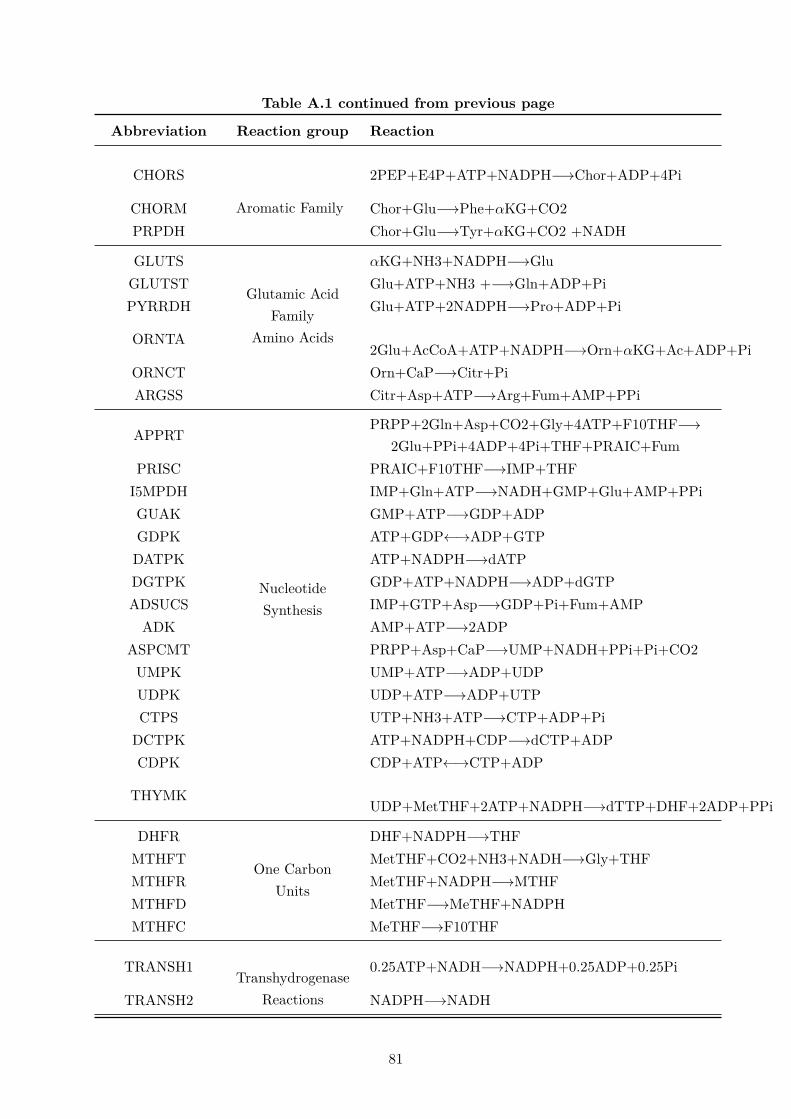
Table A.1 continued from previous page

Abbreviation Reaction group Reaction

CHORS

Aromatic Family

2PEP+E4P+ATP+NADPH−→Chor+ADP+4Pi

CHORM Chor+Glu−→Phe+αKG+CO2PRPDH Chor+Glu−→Tyr+αKG+CO2 +NADH

GLUTS

Glutamic AcidFamily

Amino Acids

αKG+NH3+NADPH−→GluGLUTST Glu+ATP+NH3 +−→Gln+ADP+PiPYRRDH Glu+ATP+2NADPH−→Pro+ADP+Pi

ORNTA2Glu+AcCoA+ATP+NADPH−→Orn+αKG+Ac+ADP+Pi

ORNCT Orn+CaP−→Citr+PiARGSS Citr+Asp+ATP−→Arg+Fum+AMP+PPi

APPRT

NucleotideSynthesis

PRPP+2Gln+Asp+CO2+Gly+4ATP+F10THF−→2Glu+PPi+4ADP+4Pi+THF+PRAIC+Fum

PRISC PRAIC+F10THF−→IMP+THFI5MPDH IMP+Gln+ATP−→NADH+GMP+Glu+AMP+PPiGUAK GMP+ATP−→GDP+ADPGDPK ATP+GDP←→ADP+GTP

DATPK ATP+NADPH−→dATPDGTPK GDP+ATP+NADPH−→ADP+dGTPADSUCS IMP+GTP+Asp−→GDP+Pi+Fum+AMP

ADK AMP+ATP−→2ADPASPCMT PRPP+Asp+CaP−→UMP+NADH+PPi+Pi+CO2

UMPK UMP+ATP−→ADP+UDPUDPK UDP+ATP−→ADP+UTPCTPS UTP+NH3+ATP−→CTP+ADP+Pi

DCTPK ATP+NADPH+CDP−→dCTP+ADPCDPK CDP+ATP←→CTP+ADP

THYMKUDP+MetTHF+2ATP+NADPH−→dTTP+DHF+2ADP+PPi

DHFR

One CarbonUnits

DHF+NADPH−→THFMTHFT MetTHF+CO2+NH3+NADH−→Gly+THFMTHFR MetTHF+NADPH−→MTHFMTHFD MetTHF−→MeTHF+NADPHMTHFC MeTHF−→F10THF

TRANSH1Transhydrogenase

Reactions

0.25ATP+NADH−→NADPH+0.25ADP+0.25Pi

TRANSH2 NADPH−→NADH

81

Table A.1 continued from previous page

Abbreviation Reaction group Reaction

ATPS1 ElectronTransport

NADH+0.5O2++2ADP+2Pi−→2ATPATPS2 FADH2+ADP+Pi+0.5O2−→ATP

GL3PD

Fatty AcidSynthesis

T3P+NADPH−→GL3P

FAS17 AcCoA + 6 ATP + 12 NADPH −→ C14:0 + 6ADP + 6 Pi

FAS27 AcCoA + 6 ATP + 11 NADPH −→ C14:0 + 6ADP + 6 Pi

FAS38.2 AcCoA + 7.2 ATP + 14 NADPH −→ FA+ 7.2ADP + 7.2 Pi

FAS4 2 ATP + CO2 + Gln −→ CaP + Glu + 2 ADP + Pi

GLUTT

Other BiomassComponents

F6P + Gln + AcCoA + UTP −→ UDPNAG + Glu+ PPi

GLCNACS PEP + NADPH + UDPNAG −→ UDPNAM + PiCMPKDOS RL5P + PEP + CTP −→ CMPKDO + PPi + 2 Pi

PPDSDCSer + CTP + ATP −→ CDPEtN + ADP + PPi+CO2

PGM2 G6P −→ G1PUTPG1PUT UTP + G1P −→ UDPGlc + PPi

BiomassProduc-tion

Biomass

0.594 Ala + 0.198 Arg + 0.143 Asn + 0.284 Asp +0.060 Cys + 0.272 Gln + 0.367 Glu + 0.495 Gly +0.086 His + 0.288 Ile + 0.368 Leu + 0.342 Lys +0.118 Met + 0.059 Orn + 0.175 Pro + 0.304 Ser +0.239 Thr + 0.335 Val +0.17 Phe + 0.13 Tyr + 0.05Trp + 0.136 UTP + 0.126 CTP + 0.203 GTP +0.0246 dATP + 0.0254 dGTP + 0.0254 dCTP +0.0246 dTTP + 0.083 GL3P + 0.0238 C14:0 +0.0238 C14:1 + 0.15 FA + 0.095 UDPNAG + 0.095UDPNAM + 0.111 UDPGlc + 0.154 + G1P+ 0.0235CMPKDO + 0.0235 CDPEtN + 22.738 ATP −→ 1gBiomass + 22.738 ADP + 22.738 Pi

ATPM Maintenance ATP−→ADP+Pi

CO2 e

TransportReactions

CO2←→expNH3 e Imp←→NH3H2S e 2ATP+4NADPH−→AMP+ADP+H2S+PPi+PiPPI PPi−→2PiPi e Imp←→Pi

82

Table A.1 continued from previous page

Abbreviation Reaction group Reaction

AA eSer+PRPP+Gln+Chor−→Trp+Glu+CO2+Pyr+T3P+Ppi

GLC e Imp−→GlcO2 e Imp−→O2

ETH e Eth−→expAC e Ac−→exp

Biomass eBiomassSynthesis

Biomass−→exp

Table A.2: List of metabolites and respective abbreviations used in the central metabolism modelnetwork. Adapted from supplementary data in Pandey et al. (2018).

Abbreviation Metabolite

Ac AcetateAcCoA Acetyl coenzyme AActn AcetoinADP Adenosine 5’ -diphosphateAla L-Alanine

AMP Adenosine 5’-monophosphateArg L-ArginineAsn L-AsparagineAsp L-Aspartate

AspSa Aspartate semialdehydeATP Adenosine 5’-triphosphateC14:0 Myristic acidC14:1 Hydroxymyristic acidCaP Carbamoyl-phosphateCDP Cytidine 5’-diphosphate

CDPEtN CDP-ethanolamineCit CitrateCitr CitrulineChor ChorismateCMP Cytidine 5’-monophosphate

CMPKDO CMP-3-deoxy-D-manno-octulosonic acidCO2 Carbon dioxideCTP Cytidine 5’-triphosphateCys L-Cysteine

dATP 2’ -Deoxy-ATPdCTP 2’ -Deoxy-CTP

83

Table A.2 continued from previous page

Abbreviation Metabolite

dGTP 2’ -Deoxy-GTPdTTP 2’ -Deoxy-TTP

DC L,2,3 dihydrodipicolinateDHF 7,8-DihydrofolateE4P Erythrose 4-phosphateEth Ethanol

F10THF N10 -Formyl-THFF6P Fructose 6-phosphate

FADH Flavine adenine dinucleotide (reduced)Fum FumarateG1P Glucose 1-phosphateG6P Glucose 6-phosphateGDP Guanosine 5’-diphosphateGL3P Glycerol 5’-phosphateGlc GlucoseGln L-GlutamineGlu L-GlutamateGluc Gluconate

Gluc6P Gluconate 6-phosphateGlx GlyoxylateGly L-Glycine

GMP Guanosine 5’-monophosphateGTP Guanosine 5’-triphosphateH2S Hydrogen sulfideHis L-Histidine

HSer HomoserineICit IsocitrateIle L-Isoleucine

IMP Inosine monophosphateaKG a-ketoglutarateKval KetovalineLeu L-LeucineLys L-LysineMal Malate

mDAP meso-DiaminopimelateMet L-Methionine

MeTHF N5-N10-methenyl-THFMetTHF N5-N10-methylene-THFMTHF N5-methyl-THFNADH Nicotinamide adenine dinucleotide (reduced)

84

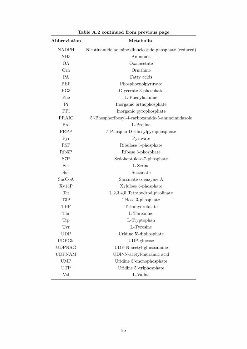
Table A.2 continued from previous page

Abbreviation Metabolite

NADPH Nicotinamide adenine dinucleotide phosphate (reduced)NH3 AmmoniaOA OxalacetateOrn OrnithinePA Fatty acids

PEP PhosphoenolpyruvatePG3 Glycerate 3-phosphatePhe L-PhenylalaninePi Inorganic orthophosphate

PPi Inorganic pyrophosphatePRAIC 5’-Phosphoribosyl-4-carboxamide-5-aminoimidazole

Pro L-ProlinePRPP 5-Phospho-D-ribosylpyrophosphate

Pyr PyruvateR5P Ribulose 5-phosphate

Rib5P Ribose 5-phosphateS7P Sedoheptulose-7-phosphateSer L-SerineSuc Succinate

SucCoA Succinate coenzyme AXy15P Xylulose 5-phosphate

Tet L,2,3,4,5 TetrahydrodipicolinateT3P Triose 3-phosphateTHF TetrahydrofolateThr L-ThreonineTrp L-TryptophanTyr L-Tyrosine

UDP Uridine 5’-diphosphateUDPGlc UDP-glucose

UDPNAG UDP-N-acetyl-glucosamineUDPNAM UDP-N-acetyl-muramic acid

UMP Uridine 5’-monophosphateUTP Uridine 5’-triphosphateVal L-Valine

85

Appendix B

Biomolecules Composition

Table B.1: Nucleotide composition of pET28a(+) sequence (that already accounts for the resistance marker sequence) added to IFNγ nucleotidic sequence(NCBI database reference sequence number AB451324.1).

Nucleotide Code MW (g/mol) # in pET28a # pET28a dS % Nucleotidic MW in pET28a (g/mol) mmole/g pET28a

dATP A 331.2 1 446 2 892 24.63 957 830.4 0.7591

dTTP T 322.2 1 395 2 790 23.76 898 938 0.7324

dGTP G 347.2 1 551 3 102 26.42 1 077 014.4 0.8143

dCTP C 307.2 1 478 2 956 25.18 9 08 083.2 0.7759

Total 5 870 11 740 100 3809630

86

Table B.2: Amino acid composition of human interferon gamma fused to an hexa-histidine affinity tag (NCBI database reference sequence number NP 000610.2- Interferon gamma precursor [homo sapiens]).

Amino acid (AA) Code MW (g/mol) MW - MW(H2O) # in IFNγ % AA MW in IFNγ (g/mol) mmole/g IFNγ

Alanine A 89.09 71.08 10 5.29 710.80 0.4587

Arginine R 174.19 156.18 9 4.76 1405.62 0.4128

Asparagine N 132.11 114.10 10 5.29 1141.00 0.4587

Aspartic Acid D 133.10 115.09 10 5.29 1150.90 0.4587

Cysteine C 121.15 103.14 3 1.59 309.42 0.1376

Glutamic acid E 147.13 129.12 9 4.76 1162.08 0.4128

Glutamine Q 146.14 128.13 10 5.29 1281.30 0.4587

Glycine G 75.06 57.05 10 5.29 570.50 0.4587

Histidine H 155.15 137.14 9 4.76 1234.26 0.4128

Isoleucine I 131.17 113.16 9 4.76 1018.44 0.4128

Leucine L 131.17 113.16 15 7.94 1697.40 0.6880

Lysine K 146.18 128.17 21 11.11 2691.57 0.9633

Methionine M 149.20 131.19 7 3.70 918.33 0.3211

Phenylalanine F 165.19 147.18 11 5.82 1618.98 0.5046

Proline P 115.13 97.12 3 1.59 291.36 0.1376

Serine S 105.09 87.08 19 10.05 1654.52 0.8715

Threonine T 119.12 101.11 6 3.17 606.66 0.2752

Typtophan W 204.22 186.21 1 0.53 186.21 0.0459

Tyrosine Y 181.19 163.18 7 3.70 1142.26 0.3211

Valine V 117.14 99.13 10 5.29 991.3 0.4587

Total 189 100 21800.92

87

Table B.3: Amino acid composition of plasmid resistance marker phosphotransferase (NCBI database reference sequence number WP 000018329 - aminoglycosideO-phosphotransferase APH(3’)-Ia [Bacteria] (kanR)).

Amino acid (AA) Code MW (g/mol) MW - MW(H2O) # in kanR % AA MW in kanR (g/mol) mmole/g kanR

Alanine A 89.09 71.08 15 5.54 1066.20 0.4842

Arginine R 174.19 156.18 16 5.90 2498.88 0.5165

Asparagine N 132.11 114.10 15 5.54 1711.50 0.4842

Aspartic Acid D 133.10 115.09 25 9.23 2877.25 0.8070

Cysteine C 121.15 103.14 5 1.85 515.70 0.1614

Glutamic acid E 147.13 129.12 13 4.80 1678.56 0.4196

Glutamine Q 146.14 128.13 10 3.69 1281.30 0.3228

Glycine G 75.06 57.05 17 6.27 969.85 0.5488

Histidine H 155.15 137.14 7 2.58 959.98 0.2260

Isoleucine I 131.17 113.16 13 4.80 1471.08 0.4196

Leucine L 131.17 113.16 29 10.70 3281.64 0.9361

Lysine K 146.18 128.17 12 4.43 1538.04 0.3874

Methionine M 149.20 131.19 8 2.95 1049.52 0.2582

Phenylalanine F 165.19 147.18 16 5.90 2354.88 0.5165

Proline P 115.13 97.12 15 5.54 1456.80 0.4842

Serine S 105.09 87.08 16 5.90 1393.28 0.5165

Threonine T 119.12 101.11 10 3.69 1011.10 0.3228

Typtophan W 204.22 186.21 6 2.21 1117.26 0.1937

Tyrosine Y 181.19 163.18 7 2.58 1142.26 0.2260

Valine V 117.14 99.13 16 5.90 1586.08 0.5165

Total 271 100 30979.17

88

Appendix C

Hierarchical Clustering Analysis

sol_394sol_344sol_83sol_84sol_1sol_304sol_303sol_302sol_301sol_300sol_299sol_298sol_297sol_296sol_295sol_294sol_293sol_292sol_291sol_290sol_289sol_288sol_287sol_286sol_285sol_284sol_283sol_282sol_280sol_279sol_278sol_277sol_276sol_275sol_274sol_273sol_272sol_271sol_270sol_268sol_269WTsol_708sol_707sol_173sol_483sol_480sol_476sol_478sol_0sol_3sol_719sol_482sol_172sol_499sol_351sol_720sol_711sol_709sol_710

05101520 Dendrogram Height

Figure C.1: Model CMM A HCA full dendrogram obtained using single linage with Euclidean distance.The colour in solution labelling refers to the colours used for the respective enumeration problems.

89

sol_271sol_1sol_2sol_3sol_31sol_313sol_343sol_309sol_820sol_628sol_4sol_60sol_310sol_312sol_486sol_311sol_629sol_632sol_631sol_630sol_316sol_314sol_315sol_213sol_139WT1WT2WT3WTWT4sol_516sol_419sol_465sol_337sol_239sol_262sol_327sol_608sol_519sol_518sol_7sol_454sol_453sol_61sol_376sol_378sol_610sol_616sol_614sol_612sol_384sol_380sol_382sol_375sol_95sol_163sol_16sol_17sol_111sol_112sol_103sol_102sol_1011sol_1001sol_100sol_101sol_458sol_457sol_456sol_4471sol_4461sol_4451sol_447sol_445sol_446sol_292sol_291sol_290sol_5342sol_5332sol_5321sol_534sol_532sol_533sol_507sol_506sol_505sol_504sol_503sol_502sol_3961sol_3951sol_3941sol_3931sol_3921sol_3911sol_396sol_395sol_394sol_393sol_391sol_392sol_538sol_537sol_5341sol_5331sol_5621sol_5611sol_5581sol_5571sol_562sol_561sol_557sol_558sol_536sol_535sol_5601sol_5591sol_559sol_560

01020 Dendrogram Height

Figure C.2: Model CMM B HCA full dendrogram obtained using single linage with Euclidean distance.The colour in solution labelling refers to the colours used for the respective enumeration problems.

90

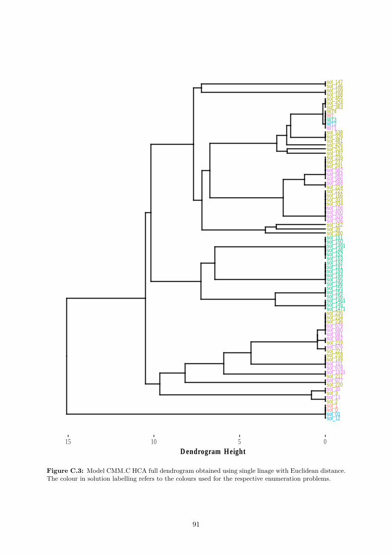
sol_12sol_01sol_0sol_1sol_2sol_11sol_3sol_31sol_220sol_677sol_217sol_1931sol_678sol_101sol_149sol_218sol_221sol_676sol_219sol_682sol_681sol_680sol_679sol_236sol_234sol_235sol_1471sol_145sol_1461sol_156sol_154sol_155sol_196sol_195sol_194sol_193sol_191sol_192sol_153sol_152sol_148sol_1491sol_150sol_151sol_280sol_39sol_162sol_536sol_535sol_400sol_106sol_334sol_333sol_166sol_222sol_224sol_588sol_586sol_584sol_582sol_241sol_237sol_239sol_197sol_514sol_426sol_481sol_329sol_538WT1WT2WT3WTWT4sol_363sol_424sol_455sol_108sol_109sol_146sol_147

051015 Dendrogram Height

Figure C.3: Model CMM C HCA full dendrogram obtained using single linage with Euclidean distance.The colour in solution labelling refers to the colours used for the respective enumeration problems.

91

sol_9sol_14sol_13sol_10sol_11sol_12sol_0sol_3sol_6sol_1sol_2sol_4sol_7sol_5sol_8sol_96sol_143sol_109sol_110sol_136sol_149sol_78sol_172sol_173sol_144sol_145sol_132sol_130sol_131sol_147sol_133sol_146sol_154sol_155sol_150sol_151sol_190sol_86sol_87sol_189sol_187sol_188sol_74sol_35sol_36sol_27sol_28sol_33sol_34sol_181sol_182sol_183sol_184sol_185sol_186sol_37sol_38sol_29sol_30sol_31sol_32sol_103sol_64sol_40sol_104sol_39sol_63sol_41sol_62sol_105sol_82sol_148sol_510sol_23sol_810sol_1110sol_22sol_410sol_710sol_1010sol_21sol_310sol_610sol_910sol_73sol_75sol_91sol_92sol_210sol_01sol_195sol_99sol_97sol_98sol_137sol_138sol_79sol_80sol_174sol_175sol_162sol_163sol_191sol_192sol_81sol_139sol_176sol_164sol_193sol_158sol_156sol_157sol_1310sol_1210sol_1410sol_18sol_56sol_1610sol_59sol_1510sol_17sol_58sol_60sol_19sol_55sol_20sol_57sol_169sol_170sol_121sol_141sol_142sol_178sol_179sol_129sol_180sol_115sol_113sol_114sol_128sol_126sol_127sol_125sol_123sol_124sol_50sol_48sol_49sol_72sol_70sol_71sol_44sol_42sol_43sol_118sol_116sol_117sol_47sol_45sol_46sol_69sol_67sol_68sol_122sol_171sol_120sol_166sol_177sol_161sol_51sol_140sol_84sol_66sol_85sol_89sol_153sol_167sol_88sol_90sol_168sol_65sol_83sol_152sol_94sol_100sol_102sol_52sol_95sol_93sol_101sol_53sol_54sol_24sol_76sol_25sol_160sol_26sol_77sol_107sol_106sol_108sol_135sol_159sol_165sol_194sol_61sol_134sol_119sol_111sol_112sol_15sol_16

0255075100 Dendrogram Height

Figure C.4: Model GSM B HCA full dendrogram obtained using single linage with Euclidean distance.The colour in solution labelling refers to the colours used for the respective enumeration problems.

92

sol_100sol_101sol_129sol_128sol_126sol_127sol_136sol_137sol_218sol_217sol_215sol_216sol_226sol_227sol_192sol_191sol_188sol_187sol_186sol_185sol_182sol_184sol_193sol_190sol_183sol_189sol_206sol_205sol_202sol_201sol_200sol_199sol_196sol_198sol_207sol_204sol_197sol_203sol_157sol_161sol_125sol_162sol_80sol_49sol_78sol_74sol_79sol_150sol_135sol_97sol_148sol_139sol_141sol_231sol_177sol_228

0255075100 Dendrogram Height

Figure C.5: Model GSM C HCA full dendrogram obtained using single linage with Euclidean distance.The colour in solution labelling refers to the colours used for the respective enumeration problems.

93