application of design-of-experiment methods and …bilicz/research/phd/phd_bilicz_pres.pdf ·...
TRANSCRIPT

Motivation,framework andobjectives
Eddy-Current Testing
Surrogate Modeling &Design-of-Experiments
Research goals
Optimization-basedinversion
Expected Improvement
Simple illustration
ENDE examples
Conclusions
Surrogate modelingby functional kriging
Adaptive sampling
Simple illustration
ENDE examples
Conclusions
Output space-filling
Adaptive sampling
Simple illustration
ENDE examples
Conclusions
Perspectives
Application of
Design-of-Experiment Methods and Surrogate Models in
Electromagnetic Nondestructive Evaluation
PhD Defense, 30 May 2011
Sándor BILICZ
“Co-tutelle” thesis
Advisors:
Marc LAMBERT and Szabolcs GYIMÓTHY
Département de Recherche en ÉlectromagnétismeLaboratoire des Signaux et Systèmes
UMR8506 (CNRS-SUPELEC-Univ Paris Sud 11)
Department of Broadband Infocommunications and Electromagnetic TheoryBudapest University of Technology and Economics
1 / 38

Motivation,framework andobjectives
Eddy-Current Testing
Surrogate Modeling &Design-of-Experiments
Research goals
Optimization-basedinversion
Expected Improvement
Simple illustration
ENDE examples
Conclusions
Surrogate modelingby functional kriging
Adaptive sampling
Simple illustration
ENDE examples
Conclusions
Output space-filling
Adaptive sampling
Simple illustration
ENDE examples
Conclusions
Perspectives
Outline
Introduction & framework
Electromagnetic Nondestructive Evaluation – illustrativeexample
Surrogate Modeling and Design-of-Experiments – some generaltools
Research goals
The backbone of the work: three independent approaches
Self-consistent entities
Same illustrative examples
Perspectives
2 / 38
Motivation,framework andobjectives
Eddy-Current Testing
Surrogate Modeling &Design-of-Experiments
Research goals
Optimization-basedinversion
Expected Improvement
Simple illustration
ENDE examples
Conclusions
Surrogate modelingby functional kriging
Adaptive sampling
Simple illustration
ENDE examples
Conclusions
Output space-filling
Adaptive sampling
Simple illustration
ENDE examples
Conclusions
Perspectives
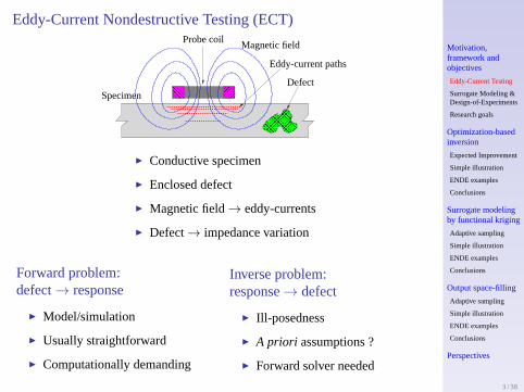
Eddy-Current Nondestructive Testing (ECT)
Probe coil
SpecimenDefect
Magnetic field
Eddy-current paths
Conductive specimen
Enclosed defect
Magnetic field→ eddy-currents
Defect→ impedance variation
Forward problem:defect→ response
Model/simulation
Usually straightforward
Computationally demanding
Inverse problem:response→ defect
Ill-posedness
A priori assumptions ?
Forward solver needed
3 / 38
Motivation,framework andobjectives
Eddy-Current Testing
Surrogate Modeling &Design-of-Experiments
Research goals
Optimization-basedinversion
Expected Improvement
Simple illustration
ENDE examples
Conclusions
Surrogate modelingby functional kriging
Adaptive sampling
Simple illustration
ENDE examples
Conclusions
Output space-filling
Adaptive sampling
Simple illustration
ENDE examples
Conclusions
Perspectives
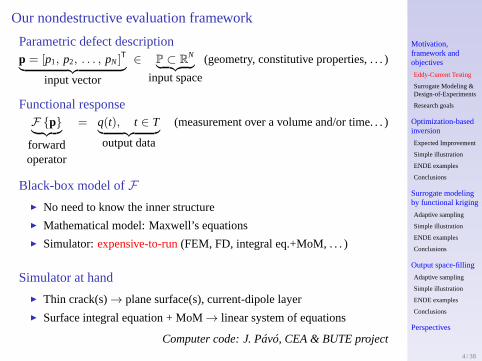
Our nondestructive evaluation framework
Parametric defect descriptionp = [p1, p2, . . . , pN]
T
︸ ︷︷ ︸input vector
∈ P ⊂ RN
︸ ︷︷ ︸input space
(geometry, constitutive properties, . . . )
Functional responseF p︸ ︷︷ ︸
forwardoperator
= q(t), t ∈ T︸ ︷︷ ︸output data
(measurement over a volume and/or time. . . )
Black-box model ofF
No need to know the inner structure Mathematical model: Maxwell’s equations Simulator:expensive-to-run(FEM, FD, integral eq.+MoM, . . . )
Simulator at hand
Thin crack(s)→ plane surface(s), current-dipole layer
Surface integral equation + MoM→ linear system of equations
Computer code: J. Pávó, CEA & BUTE project4 / 38
Motivation,framework andobjectives
Eddy-Current Testing
Surrogate Modeling &Design-of-Experiments
Research goals
Optimization-basedinversion
Expected Improvement
Simple illustration
ENDE examples
Conclusions
Surrogate modelingby functional kriging
Adaptive sampling
Simple illustration
ENDE examples
Conclusions
Output space-filling
Adaptive sampling
Simple illustration
ENDE examples
Conclusions
Perspectives
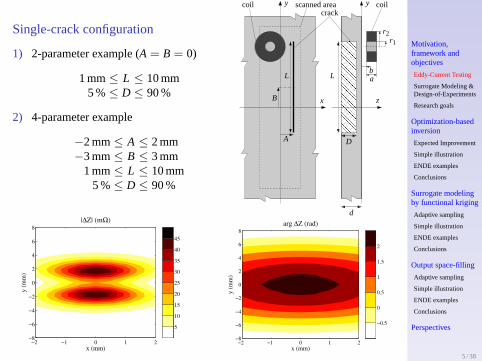
Single-crack configuration
1) 2-parameter example (A = B = 0)
1 mm≤ L ≤ 10 mm5 %≤ D ≤ 90 %
2) 4-parameter example
−2 mm≤ A ≤ 2 mm−3 mm≤ B ≤ 3 mm
1 mm≤ L ≤ 10 mm5 %≤ D ≤ 90 %
r1
r2
ba
x
yy
z
L L
DA
B
d
coilcoilcrack
scanned area
|∆Z| (mΩ)
x (mm)
y (
mm
)
−2 −1 0 1 2−8
−6
−4
−2
0
2
4
6
8
5
10
15
20
25
30
35
40
45
arg ∆Z (rad)
x (mm)
y (
mm
)
−2 −1 0 1 2−8
−6
−4
−2
0
2
4
6
8
−0.5
0
0.5
1
1.5
2
5 / 38

Motivation,framework andobjectives
Eddy-Current Testing
Surrogate Modeling &Design-of-Experiments
Research goals
Optimization-basedinversion
Expected Improvement
Simple illustration
ENDE examples
Conclusions
Surrogate modelingby functional kriging
Adaptive sampling
Simple illustration
ENDE examples
Conclusions
Output space-filling
Adaptive sampling
Simple illustration
ENDE examples
Conclusions
Perspectives
Double-crack configuration
3) 6-parameter example (D1 = D2 = 40 %)
−1 mm≤ A ≤ 1 mm0.25 mm≤ h ≤ 2 mm−3 mm≤ B1,B2 ≤ 3 mm
1 mm≤ L1, L2 ≤ 10 mm
4) 8-parameter example
−1 mm≤ A ≤ 1 mm0.25 mm≤ h ≤ 2 mm−3 mm≤ B1,B2 ≤ 3 mm
1 mm≤ L1, L2 ≤ 10 mm5 %≤ D1,D2 ≤ 80 %
r1
r2
ba
x
yy
zA
d
L1L1
D1
h
B1
L2L2
D2
B2
coilcoilcrack
scanned area
|∆Z| (mΩ)
x (mm)
y (
mm
)
−2 −1 0 1 2−8
−6
−4
−2
0
2
4
6
8
10
20
30
40
50
60
70
80
90
100
arg ∆Z (rad)
x (mm)
y (
mm
)
−2 −1 0 1 2−8
−6
−4
−2
0
2
4
6
8
0
0.2
0.4
0.6
0.8
1
1.2
1.4
1.6
1.8
6 / 38

Motivation,framework andobjectives
Eddy-Current Testing
Surrogate Modeling &Design-of-Experiments
Research goals
Optimization-basedinversion
Expected Improvement
Simple illustration
ENDE examples
Conclusions
Surrogate modelingby functional kriging
Adaptive sampling
Simple illustration
ENDE examples
Conclusions
Output space-filling
Adaptive sampling
Simple illustration
ENDE examples
Conclusions
Perspectives
Surrogate Modeling (SM) and Design-of-Experiments (DoE)
“Expensive” true modelF
SurrogateModeling
−−−−−−−−−→ Approximate modelF Reducing computational complexity
(CPU, memory, price of commercial code, . . . )
Often interpolation supported by some pre-computed results
Fp1, Fp2, . . . , Fpn −→ Fp
Criterion: “small error” using “few” samples
Choice ofp1, p2, . . . , pn −→ Design-of-Experiments Systematically performing observations for a specific purpose
n = ? Error = ?
“Real” experiments / computer simulations
Classical methods (pi )
Model-oriented methods (pi , F )
Adaptive methods (pi , F , Fpi )
7 / 38

Motivation,framework andobjectives
Eddy-Current Testing
Surrogate Modeling &Design-of-Experiments
Research goals
Optimization-basedinversion
Expected Improvement
Simple illustration
ENDE examples
Conclusions
Surrogate modelingby functional kriging
Adaptive sampling
Simple illustration
ENDE examples
Conclusions
Output space-filling
Adaptive sampling
Simple illustration
ENDE examples
Conclusions
Perspectives
Sampling by means of classical Design-of-Experiments
Goals
filling “well” P by the samplesp1, p2, . . . , pn
representing “well” the effect of each coordinate ofP
. . .
Examples
Full-Factorial (FF) design:K levels inN dimensions:n = KN
Latin Hypercube (LH) design:n intervals along each axis→ n points
8 / 38
Motivation,framework andobjectives
Eddy-Current Testing
Surrogate Modeling &Design-of-Experiments
Research goals
Optimization-basedinversion
Expected Improvement
Simple illustration
ENDE examples
Conclusions
Surrogate modelingby functional kriging
Adaptive sampling
Simple illustration
ENDE examples
Conclusions
Output space-filling
Adaptive sampling
Simple illustration
ENDE examples
Conclusions
Perspectives
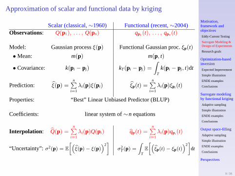
Approximation of scalar and functional data by kriging
Scalar (classical,∼1960) Functional (recent,∼2004)Observations: Q(p1), . . . , Q(pn) qp1(t), . . . , qpn(t)
Model: Gaussian processξ(p) Functional Gaussian proc.ξp(t)
• Mean: m(p) m(p, t)
• Covariance: k(pi − pj) kT(pi − pj) =
∫
Tk(pi − pj , t)dt
Prediction: ξ(p) =n∑
i=1λi(p)ξ(pi) ξp(t) =
n∑i=1
λi(p)ξpi (t)
Properties: “Best” Linear Unbiased Predictor (BLUP)
Coefficients: linear system of∼n equations
Interpolation : Q(p) =n∑
i=1λi(p)Q(pi) qp(t) =
n∑i=1
λi(p)qpi (t)
“Uncertainty”: σ2(p) = E
[(ξ(p)− ξ(p)
)2]
σ2T(p) =
∫
TE
[(ξp(t)− ξp(t)
)2]
dt
9 / 38

Motivation,framework andobjectives
Eddy-Current Testing
Surrogate Modeling &Design-of-Experiments
Research goals
Optimization-basedinversion
Expected Improvement
Simple illustration
ENDE examples
Conclusions
Surrogate modelingby functional kriging
Adaptive sampling
Simple illustration
ENDE examples
Conclusions
Output space-filling
Adaptive sampling
Simple illustration
ENDE examples
Conclusions
Perspectives
Choice of the covariance
Parametric covariance model: the Matérn function
k(h |σ20, ν) = σ
20(2√ν h)ν Kν(2
√ν h)
2ν−1Γ(ν), h =
√√√√ N∑k=1
(p(k)
i − p(k)j
ρi
)2
Variance:σ20
Smoothness:ν
Scaling factors:ρ1, ρ2, . . . , ρN →anisotropic distance
more. . .
0 0.2 0.4 0.6 0.8 10
0.2
0.4
0.6
0.8
1
ν = 0.25
ν = 1
ν = 4
hρ (ρ = 0.25)
k(h)
Estimation of the parameters:
(Restricted) Maximum Likelihood
Cross-Validation
Numerical implementation (partly) by E. Vazquez, Supélec10 / 38
Motivation,framework andobjectives
Eddy-Current Testing
Surrogate Modeling &Design-of-Experiments
Research goals
Optimization-basedinversion
Expected Improvement
Simple illustration
ENDE examples
Conclusions
Surrogate modelingby functional kriging
Adaptive sampling
Simple illustration
ENDE examples
Conclusions
Output space-filling
Adaptive sampling
Simple illustration
ENDE examples
Conclusions
Perspectives
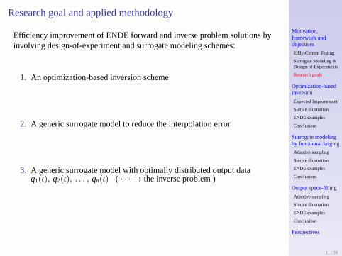
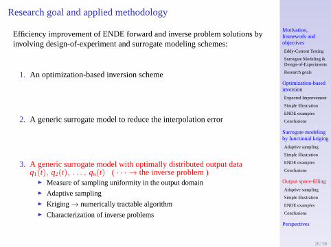
Research goal and applied methodology
Efficiency improvement of ENDE forward and inverse problem solutions byinvolving design-of-experiment and surrogate modeling schemes:
1. An optimization-based inversion scheme
2. A generic surrogate model to reduce the interpolation error
3. A generic surrogate model with optimally distributed output dataq1(t), q2(t), . . . , qn(t) ( · · · → the inverse problem )
11 / 38
Motivation,framework andobjectives
Eddy-Current Testing
Surrogate Modeling &Design-of-Experiments
Research goals
Optimization-basedinversion
Expected Improvement
Simple illustration
ENDE examples
Conclusions
Surrogate modelingby functional kriging
Adaptive sampling
Simple illustration
ENDE examples
Conclusions
Output space-filling
Adaptive sampling
Simple illustration
ENDE examples
Conclusions
Perspectives
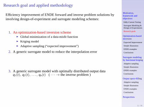
Research goal and applied methodology
Efficiency improvement of ENDE forward and inverse problem solutions byinvolving design-of-experiment and surrogate modeling schemes:
1. An optimization-based inversion scheme Global minimization of a data-misfit function Kriging model Adaptive sampling (“expected improvement”)
2. A generic surrogate model to reduce the interpolation error
3. A generic surrogate model with optimally distributed output dataq1(t), q2(t), . . . , qn(t) ( · · · → the inverse problem )
11 / 38

Motivation,framework andobjectives
Eddy-Current Testing
Surrogate Modeling &Design-of-Experiments
Research goals
Optimization-basedinversion
Expected Improvement
Simple illustration
ENDE examples
Conclusions
Surrogate modelingby functional kriging
Adaptive sampling
Simple illustration
ENDE examples
Conclusions
Output space-filling
Adaptive sampling
Simple illustration
ENDE examples
Conclusions
Perspectives
Optimization-based inversion
Measured data:q(t)
Parametric model:q(t) = Fp Data-misfit→ objective function:Q(p) = ‖q(t)−Fp‖ The regularized inverse problem:
p⋆ = arg minp∈P
Q(p)
Simulator
Measurement Strategy
q(t)
Fpp
Q(p)
Challenges:Q(p) expensive-to-evaluate
might be multimodal
−→ “Efficient Global Optimization”
kriging model (Surrogate Model)
sequential sampling (DoE)
12 / 38

Motivation,framework andobjectives
Eddy-Current Testing
Surrogate Modeling &Design-of-Experiments
Research goals
Optimization-basedinversion
Expected Improvement
Simple illustration
ENDE examples
Conclusions
Surrogate modelingby functional kriging
Adaptive sampling
Simple illustration
ENDE examples
Conclusions
Output space-filling
Adaptive sampling
Simple illustration
ENDE examples
Conclusions
Perspectives
The “Expected Improvement” sampling criterion
Sequential sampling for the solution of
p⋆ = arg minp∈P
Q(p), p1, p2, p3, . . . p⋆
0. Initial observations:Q(p1), Q(p2), . . . , Q(pn)
1. Qmin = min[Q(p1), . . . , Q(pn)
]
2. Kriging prediction:ξ(p) ∈ N(
Q(p), σ2(p))
(normally distributed)
Improvement atp by evaluatingQ there:I(p) = Qmin − ξ(p)
“Expected Improvement” atp:
η(p) := E
[I(p)
∣∣∣ I(p) > 0]
closed-form expression available
3. The next evaluation:pn+1 = arg max
p∈Pη(p)
4. Update the model withQ(pn+1). UNTIL the stopping criterion is met,increasen := n+ 1 and GOTO step1.
13 / 38

Motivation,framework andobjectives
Eddy-Current Testing
Surrogate Modeling &Design-of-Experiments
Research goals
Optimization-basedinversion
Expected Improvement
Simple illustration
ENDE examples
Conclusions
Surrogate modelingby functional kriging
Adaptive sampling
Simple illustration
ENDE examples
Conclusions
Output space-filling
Adaptive sampling
Simple illustration
ENDE examples
Conclusions
Perspectives
A simple illustrationHigh expected improvement:
Low Q(p) : “promising” p
High σ2(p) : “unexplored”p ⇒ Balanced local/global search
14 / 38

Motivation,framework andobjectives
Eddy-Current Testing
Surrogate Modeling &Design-of-Experiments
Research goals
Optimization-basedinversion
Expected Improvement
Simple illustration
ENDE examples
Conclusions
Surrogate modelingby functional kriging
Adaptive sampling
Simple illustration
ENDE examples
Conclusions
Output space-filling
Adaptive sampling
Simple illustration
ENDE examples
Conclusions
Perspectives
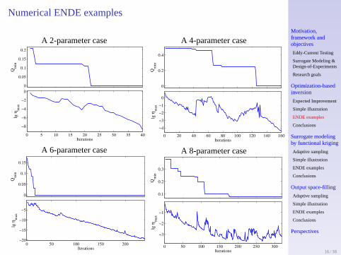
Numerical ENDE examples Normalized misfit function:Q(p) =
‖q(t)−Fp‖‖q(t)‖
Synthetic data ( ) Initial samples (N ): Latin Hypercube design Sequential sampling (• ) until n = nmax
N 2 4 6 8ninit 10 40 60 80nmax 40 160 240 320
A 2-parameter example (L = 2.5 mm,D = 75 %)
15 / 38
Motivation,framework andobjectives
Eddy-Current Testing
Surrogate Modeling &Design-of-Experiments
Research goals
Optimization-basedinversion
Expected Improvement
Simple illustration
ENDE examples
Conclusions
Surrogate modelingby functional kriging
Adaptive sampling
Simple illustration
ENDE examples
Conclusions
Output space-filling
Adaptive sampling
Simple illustration
ENDE examples
Conclusions
Perspectives
Numerical ENDE examples
A 2-parameter case
0
0.05
0.1
0.15
0.2
Qm
in
0 5 10 15 20 25 30 35 40
−8
−6
−4
−2
0
Iterations
lg η
max
A 6-parameter case
0
0.05
0.1
0.15
Qm
in
0 50 100 150 200−20
−15
−10
−5
Iterations
lg η
max
A 4-parameter case
0
0.2
0.4
Qm
in
0 20 40 60 80 100 120 140 160
−4
−3
−2
−1
0
Iterations
lg η
max
A 8-parameter case
0.1
0.2
0.3
Qm
in
0 50 100 150 200 250 300
−3
−2
−1
Iterations
lg η
max
16 / 38

Motivation,framework andobjectives
Eddy-Current Testing
Surrogate Modeling &Design-of-Experiments
Research goals
Optimization-basedinversion
Expected Improvement
Simple illustration
ENDE examples
Conclusions
Surrogate modelingby functional kriging
Adaptive sampling
Simple illustration
ENDE examples
Conclusions
Output space-filling
Adaptive sampling
Simple illustration
ENDE examples
Conclusions
Perspectives
Conclusions
Pros
Usually “few” iterations F is black-box→ generalization Gradient-free Implementation:
→ access to the precision ofdefect reconstruction
Cons
Not always few iterations Initial design ? Stopping criteria ? Gradient-free “Curse-of-Dimensionality”
Covariance parameters Exponential increase ofP
Perspectives
Gradient available: improved kriging model / stopping criterion
Combined stopping criteria (n, Qmin, ηmax)
Two-stage optimization
Related articleS. Bilicz, E. Vazquez, M. Lambert, Sz. Gyimóthy, and J. Pávó,“Characterization of a 3D defect using the Expected Improvement algorithm,”COMPEL, 28(4), pp. 851-864, 2009.
17 / 38
Motivation,framework andobjectives
Eddy-Current Testing
Surrogate Modeling &Design-of-Experiments
Research goals
Optimization-basedinversion
Expected Improvement
Simple illustration
ENDE examples
Conclusions
Surrogate modelingby functional kriging
Adaptive sampling
Simple illustration
ENDE examples
Conclusions
Output space-filling
Adaptive sampling
Simple illustration
ENDE examples
Conclusions
Perspectives
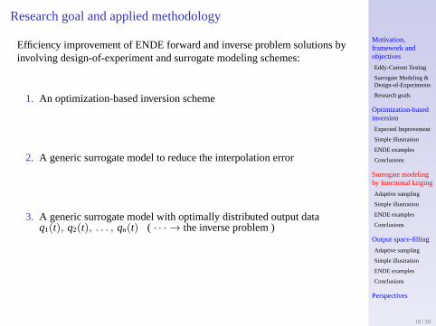
Research goal and applied methodology
Efficiency improvement of ENDE forward and inverse problem solutions byinvolving design-of-experiment and surrogate modeling schemes:
1. An optimization-based inversion scheme
2. A generic surrogate model to reduce the interpolation error
3. A generic surrogate model with optimally distributed output dataq1(t), q2(t), . . . , qn(t) ( · · · → the inverse problem )
18 / 38

Motivation,framework andobjectives
Eddy-Current Testing
Surrogate Modeling &Design-of-Experiments
Research goals
Optimization-basedinversion
Expected Improvement
Simple illustration
ENDE examples
Conclusions
Surrogate modelingby functional kriging
Adaptive sampling
Simple illustration
ENDE examples
Conclusions
Output space-filling
Adaptive sampling
Simple illustration
ENDE examples
Conclusions
Perspectives
Research goal and applied methodology
Efficiency improvement of ENDE forward and inverse problem solutions byinvolving design-of-experiment and surrogate modeling schemes:
1. An optimization-based inversion scheme
2. A generic surrogate model to reduce the interpolation error Functional kriging model ofF Error estimation in a statistical framework Adaptive sampling
3. A generic surrogate model with optimally distributed output dataq1(t), q2(t), . . . , qn(t) ( · · · → the inverse problem )
18 / 38

Motivation,framework andobjectives
Eddy-Current Testing
Surrogate Modeling &Design-of-Experiments
Research goals
Optimization-basedinversion
Expected Improvement
Simple illustration
ENDE examples
Conclusions
Surrogate modelingby functional kriging
Adaptive sampling
Simple illustration
ENDE examples
Conclusions
Output space-filling
Adaptive sampling
Simple illustration
ENDE examples
Conclusions
Perspectives
Interpolation-based generic surrogate modeling
A 2-stage approach
1. Database:Dn =(p1, q1(t)) , . . . , (pn, qn(t))
, qi(t) = Fpi
time-consuming, performed onlyonceby “experts”
2. Interpolation:Fp ≃ Fp, ∀p ∈ P and Fpi ≡ Fpi, ∀pi
“real-time”, performed by the“end-user”
Properties
Error: ε(p) = ‖Fp − Fp‖,
with a function norm, e.g.:‖·‖ ≡√
1|T|
∫
T
| · |2dt
General purpose→ general criteria forε(p) all overP :
εmax = maxp∈P
ε(p), εRMS =
√1|P|
∫
p∈P
ε2(p)dp, . . .
Reducedn, as far as possible
19 / 38
Motivation,framework andobjectives
Eddy-Current Testing
Surrogate Modeling &Design-of-Experiments
Research goals
Optimization-basedinversion
Expected Improvement
Simple illustration
ENDE examples
Conclusions
Surrogate modelingby functional kriging
Adaptive sampling
Simple illustration
ENDE examples
Conclusions
Output space-filling
Adaptive sampling
Simple illustration
ENDE examples
Conclusions
Perspectives
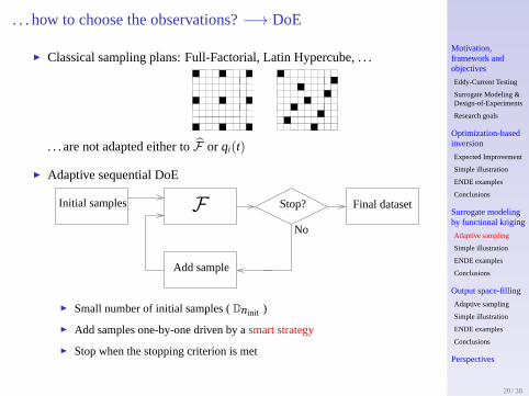
. . . how to choose the observations?−→ DoE
Classical sampling plans: Full-Factorial, Latin Hypercube, . . .
. . . are not adapted either toF or qi(t)
Adaptive sequential DoE
Initial samples F
Add sample
No
Stop? Final dataset
Small number of initial samples (Dninit )
Add samples one-by-one driven by asmart strategy
Stop when the stopping criterion is met
20 / 38

Motivation,framework andobjectives
Eddy-Current Testing
Surrogate Modeling &Design-of-Experiments
Research goals
Optimization-basedinversion
Expected Improvement
Simple illustration
ENDE examples
Conclusions
Surrogate modelingby functional kriging
Adaptive sampling
Simple illustration
ENDE examples
Conclusions
Output space-filling
Adaptive sampling
Simple illustration
ENDE examples
Conclusions
Perspectives
Sequential sampling strategy:p1, p2, . . . , pn → pn+1 =???
Implicit formulas
pn+1 = arg minp∈P
[ε(n+1)max
], pn+1 = arg min
p∈P
[ε(n+1)RMS
], . . .
Towards realizable explicit approximations
pn+1 = arg maxp∈P
[ε(n)(p)
]still computationally intractable. . .
Variance-driven sampling: Kriging (trace) varianceσ2
T(p) ∼ interpolation errorε(p)
Use the “jackknife-variance”σ2T,Jack(p)
more. . .
Naive sampling:
pn+1 = arg maxp∈P
[σ2
T,Jack(p)]
Two-factor product (heuristic):
pn+1 = arg maxp∈P
[σ2
T,Jack(p)︸ ︷︷ ︸“adaptivity”
factor
× mini=1,2,...,n
‖p − pi‖
︸ ︷︷ ︸input space-filling
]
21 / 38

Motivation,framework andobjectives
Eddy-Current Testing
Surrogate Modeling &Design-of-Experiments
Research goals
Optimization-basedinversion
Expected Improvement
Simple illustration
ENDE examples
Conclusions
Surrogate modelingby functional kriging
Adaptive sampling
Simple illustration
ENDE examples
Conclusions
Output space-filling
Adaptive sampling
Simple illustration
ENDE examples
Conclusions
Perspectives
A simple illustration:R 7→ R polynomial function (not functional kriging)
Auxiliary function: Q(p) = σ2T,Jack(p)× min
i=1,2,...,n‖p− pi‖
22 / 38

Motivation,framework andobjectives
Eddy-Current Testing
Surrogate Modeling &Design-of-Experiments
Research goals
Optimization-basedinversion
Expected Improvement
Simple illustration
ENDE examples
Conclusions
Surrogate modelingby functional kriging
Adaptive sampling
Simple illustration
ENDE examples
Conclusions
Output space-filling
Adaptive sampling
Simple illustration
ENDE examples
Conclusions
Perspectives
Numerical ENDE examples
Initial samples: a classical input space-filling (Fractional-Factorial)
Stopping criterion:n = nmax
Comparisons:
Adaptive sampling +functional kriging
1 2 3 4 5 6 7 8 9 105
20
40
55
75
90
L (mm)
D(%
)
Full-factorial sampling +multilinear interpolator
1 2 3 4 5 6 7 8 9 105
20
40
55
75
90
L (mm)
D(%
)Full-factorial sampling +
functional kriging
1 2 3 4 5 6 7 8 9 105
20
40
55
75
90
2
4
6
8
10
L (mm)D
(%)
ε(p) is evaluated at a finite number of test points
εmax andεRMS are approximately computed
23 / 38

Motivation,framework andobjectives
Eddy-Current Testing
Surrogate Modeling &Design-of-Experiments
Research goals
Optimization-basedinversion
Expected Improvement
Simple illustration
ENDE examples
Conclusions
Surrogate modelingby functional kriging
Adaptive sampling
Simple illustration
ENDE examples
Conclusions
Output space-filling
Adaptive sampling
Simple illustration
ENDE examples
Conclusions
Perspectives
The 2-parameter example
9 16 25 360
5
10
15
20
25
30
Samples
εm
ax (
mΩ
)
Kriging full−fact.
Kriging adaptive
Multilinear
9 16 25 360
1
2
3
4
5
6
7
8
9
Samples
εR
MS (
mΩ
)
Kriging full−fact.
Kriging adaptive
Multilinear
The 4-parameter example
81 144 2565
10
15
20
25
30
35
Samples
εm
ax (
mΩ
)
Kriging full−fact.
Kriging adaptive I
Kriging adaptive II
Multilinear
81 144 2562
3
4
5
6
7
8
9
10
Samples
εR
MS (
mΩ
)
Kriging full−fact.
Kriging adaptive I
Kriging adaptive II
Multilinear
24 / 38
Motivation,framework andobjectives
Eddy-Current Testing
Surrogate Modeling &Design-of-Experiments
Research goals
Optimization-basedinversion
Expected Improvement
Simple illustration
ENDE examples
Conclusions
Surrogate modelingby functional kriging
Adaptive sampling
Simple illustration
ENDE examples
Conclusions
Output space-filling
Adaptive sampling
Simple illustration
ENDE examples
Conclusions
Perspectives
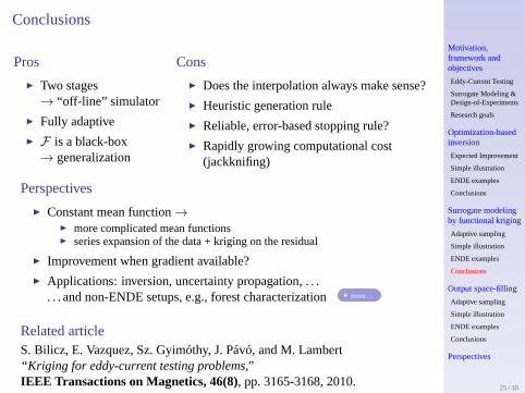
Conclusions
Pros
Two stages→ “off-line” simulator
Fully adaptive
F is a black-box→ generalization
Cons
Does the interpolation always make sense?
Heuristic generation rule
Reliable, error-based stopping rule?
Rapidly growing computational cost(jackknifing)
Perspectives
Constant mean function→ more complicated mean functions series expansion of the data + kriging on the residual
Improvement when gradient available?
Applications: inversion, uncertainty propagation, . . .. . . and non-ENDE setups, e.g., forest characterizationmore. . .
Related articleS. Bilicz, E. Vazquez, Sz. Gyimóthy, J. Pávó, and M. Lambert“Kriging for eddy-current testing problems,”IEEE Transactions on Magnetics, 46(8), pp. 3165-3168, 2010.
25 / 38

Motivation,framework andobjectives
Eddy-Current Testing
Surrogate Modeling &Design-of-Experiments
Research goals
Optimization-basedinversion
Expected Improvement
Simple illustration
ENDE examples
Conclusions
Surrogate modelingby functional kriging
Adaptive sampling
Simple illustration
ENDE examples
Conclusions
Output space-filling
Adaptive sampling
Simple illustration
ENDE examples
Conclusions
Perspectives
Research goal and applied methodology
Efficiency improvement of ENDE forward and inverse problem solutions byinvolving design-of-experiment and surrogate modeling schemes:
1. An optimization-based inversion scheme
2. A generic surrogate model to reduce the interpolation error
3. A generic surrogate model with optimally distributed output dataq1(t), q2(t), . . . , qn(t) ( · · · → the inverse problem )
26 / 38
Motivation,framework andobjectives
Eddy-Current Testing
Surrogate Modeling &Design-of-Experiments
Research goals
Optimization-basedinversion
Expected Improvement
Simple illustration
ENDE examples
Conclusions
Surrogate modelingby functional kriging
Adaptive sampling
Simple illustration
ENDE examples
Conclusions
Output space-filling
Adaptive sampling
Simple illustration
ENDE examples
Conclusions
Perspectives
Research goal and applied methodology
Efficiency improvement of ENDE forward and inverse problem solutions byinvolving design-of-experiment and surrogate modeling schemes:
1. An optimization-based inversion scheme
2. A generic surrogate model to reduce the interpolation error
3. A generic surrogate model with optimally distributed output dataq1(t), q2(t), . . . , qn(t) ( · · · → the inverse problem )
Measure of sampling uniformity in the output domain Adaptive sampling Kriging → numerically tractable algorithm Characterization of inverse problems
26 / 38

Motivation,framework andobjectives
Eddy-Current Testing
Surrogate Modeling &Design-of-Experiments
Research goals
Optimization-basedinversion
Expected Improvement
Simple illustration
ENDE examples
Conclusions
Surrogate modelingby functional kriging
Adaptive sampling
Simple illustration
ENDE examples
Conclusions
Output space-filling
Adaptive sampling
Simple illustration
ENDE examples
Conclusions
Perspectives
Spaces, sampling, space-filling
RN ⊃ P︸︷︷︸inputspace
∋ p 7→ Fp = q(t) ∈ Q︸︷︷︸outputspace
⊂ L2(T)
SamplingDn =
(p1, q1(t)) , (p2, q2(t)) , . . . , (pn, qn(t))
, qi(t) = Fpi
a discrete representation ofF
Repartition of samples inP andQ → properties of representation
Input space-filling: classical DoE (Full-factorial, Latin hypercube, . .. )
Output space-filling: adaptive DoE Criteria forq1(t), q2(t), . . . , qn(t)
Inherently more difficult (F : P 7→ Q )
Iterative / incremental realization
Our proposal: a combined use of two distance-based criteria
27 / 38

Motivation,framework andobjectives
Eddy-Current Testing
Surrogate Modeling &Design-of-Experiments
Research goals
Optimization-basedinversion
Expected Improvement
Simple illustration
ENDE examples
Conclusions
Surrogate modelingby functional kriging
Adaptive sampling
Simple illustration
ENDE examples
Conclusions
Output space-filling
Adaptive sampling
Simple illustration
ENDE examples
Conclusions
Perspectives
Output space-filling. . . How and why?
Our criteria forq1(t), q2(t), . . . , qn(t)
1. Fill the wholeQ: maxq(t)∈Q
[min
i‖q(t)− qi(t)‖
]< ∆
2. With evenly spaced samples:max
i
[minj 6=i
‖qi(t)− qj(t)‖]
mini
[minj 6=i
‖qi(t)− qj(t)‖] = 1
Expected benefits of such output space-filling databases
Addressing the inverse problem:
Higher precision due to the better describedQ
“Meta-information” from the structure of such database
→ Characterization of the inverse problem
28 / 38
Motivation,framework andobjectives
Eddy-Current Testing
Surrogate Modeling &Design-of-Experiments
Research goals
Optimization-basedinversion
Expected Improvement
Simple illustration
ENDE examples
Conclusions
Surrogate modelingby functional kriging
Adaptive sampling
Simple illustration
ENDE examples
Conclusions
Output space-filling
Adaptive sampling
Simple illustration
ENDE examples
Conclusions
Perspectives
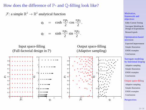
How does the difference ofP- andQ-filling look like?
F : a simpleR2 → R2 analytical function
q1 = coshπp1
2cos
πp2
2,
q2 = sinhπp1
2sin
πp2
2.
Input space-filling(Full-factorial design inP)
0 0.5 10
0.1
0.2
0.3
0.4
0.5
0.6
0.7
0.8
0.9
1
0 1 2 30
0.5
1
1.5
2
2.5
p1
p 2
q1
q 2
Output space-filling(Adaptive sampling)
0 0.5 10
0.1
0.2
0.3
0.4
0.5
0.6
0.7
0.8
0.9
1
0 1 2 30
0.5
1
1.5
2
2.5
p1
p 2
q1
q 2
29 / 38
Motivation,framework andobjectives
Eddy-Current Testing
Surrogate Modeling &Design-of-Experiments
Research goals
Optimization-basedinversion
Expected Improvement
Simple illustration
ENDE examples
Conclusions
Surrogate modelingby functional kriging
Adaptive sampling
Simple illustration
ENDE examples
Conclusions
Output space-filling
Adaptive sampling
Simple illustration
ENDE examples
Conclusions
Perspectives
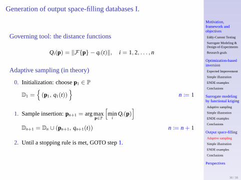
Generation of output space-filling databases I.
Governing tool: the distance functions
Qi(p) = ‖Fp − qi(t)‖, i = 1, 2, . . . , n
Adaptive sampling (in theory)
0. Initialization: choosep1 ∈ P
D1 =(p1, q1(t))
n := 1
1. Sample insertion:pn+1 = arg maxp∈P
[min
iQi(p)
]
Dn+1 = Dn ∪ (pn+1, qn+1(t)) n := n+ 1
2. Until a stopping rule is met, GOTO step1.
30 / 38
Motivation,framework andobjectives
Eddy-Current Testing
Surrogate Modeling &Design-of-Experiments
Research goals
Optimization-basedinversion
Expected Improvement
Simple illustration
ENDE examples
Conclusions
Surrogate modelingby functional kriging
Adaptive sampling
Simple illustration
ENDE examples
Conclusions
Output space-filling
Adaptive sampling
Simple illustration
ENDE examples
Conclusions
Perspectives
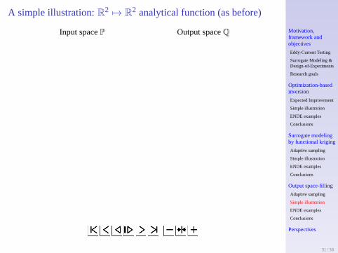
A simple illustration:R27→ R2 analytical function (as before)
Input spaceP Output spaceQ
31 / 38

Motivation,framework andobjectives
Eddy-Current Testing
Surrogate Modeling &Design-of-Experiments
Research goals
Optimization-basedinversion
Expected Improvement
Simple illustration
ENDE examples
Conclusions
Surrogate modelingby functional kriging
Adaptive sampling
Simple illustration
ENDE examples
Conclusions
Output space-filling
Adaptive sampling
Simple illustration
ENDE examples
Conclusions
Perspectives
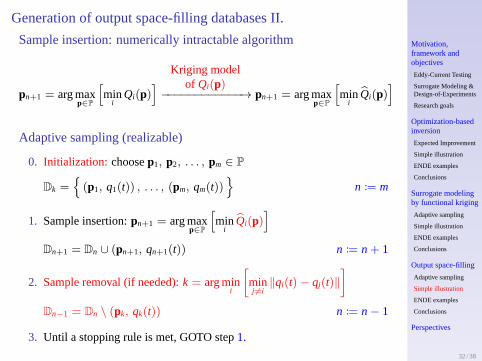
Generation of output space-filling databases II.
Sample insertion: numerically intractable algorithm
pn+1 = arg maxp∈P
[min
iQi(p)
]Kriging model
of Qi(p)−−−−−−−−−−−−→ pn+1 = arg maxp∈P
[min
iQi(p)
]
Adaptive sampling (realizable)
0. Initialization: choosep1, p2, . . . , pm ∈ P
Dk =(p1, q1(t)) , . . . , (pm, qm(t))
n := m
1. Sample insertion:pn+1 = arg maxp∈P
[min
iQi(p)
]
Dn+1 = Dn ∪ (pn+1, qn+1(t)) n := n+ 1
2. Sample removal (if needed):k = arg mini
[minj 6=i
‖qi(t)− qj(t)‖]
Dn−1 = Dn \ (pk, qk(t)) n := n− 1
3. Until a stopping rule is met, GOTO step1.
32 / 38
Motivation,framework andobjectives
Eddy-Current Testing
Surrogate Modeling &Design-of-Experiments
Research goals
Optimization-basedinversion
Expected Improvement
Simple illustration
ENDE examples
Conclusions
Surrogate modelingby functional kriging
Adaptive sampling
Simple illustration
ENDE examples
Conclusions
Output space-filling
Adaptive sampling
Simple illustration
ENDE examples
Conclusions
Perspectives
Generation of output space-filling databases II.
Sample insertion: numerically intractable algorithm
pn+1 = arg maxp∈P
[min
iQi(p)
]Kriging model
of Qi(p)−−−−−−−−−−−−→ pn+1 = arg maxp∈P
[min
iQi(p)
]
Adaptive sampling (realizable)
0. Initialization: choosep1, p2, . . . , pm ∈ P
Dk =(p1, q1(t)) , . . . , (pm, qm(t))
n := m
1. Sample insertion:pn+1 = arg maxp∈P
[min
iQi(p)
]
Dn+1 = Dn ∪ (pn+1, qn+1(t)) n := n+ 1
2. Sample removal (if needed):k = arg mini
[minj 6=i
‖qi(t)− qj(t)‖]
Dn−1 = Dn \ (pk, qk(t)) n := n− 1
3. Until a stopping rule is met, GOTO step1.
32 / 38

Motivation,framework andobjectives
Eddy-Current Testing
Surrogate Modeling &Design-of-Experiments
Research goals
Optimization-basedinversion
Expected Improvement
Simple illustration
ENDE examples
Conclusions
Surrogate modelingby functional kriging
Adaptive sampling
Simple illustration
ENDE examples
Conclusions
Output space-filling
Adaptive sampling
Simple illustration
ENDE examples
Conclusions
Perspectives
The sampling algorithm
Kriging prediction
Initial observationsStart
N
New observation
Remove?Stop?End
N
Remove sample
Initial observations: classical input space-filling
Sample removal: in every second cycle (other rules can also be applied)
Stopping rule:n = nmax
33 / 38

Motivation,framework andobjectives
Eddy-Current Testing
Surrogate Modeling &Design-of-Experiments
Research goals
Optimization-basedinversion
Expected Improvement
Simple illustration
ENDE examples
Conclusions
Surrogate modelingby functional kriging
Adaptive sampling
Simple illustration
ENDE examples
Conclusions
Output space-filling
Adaptive sampling
Simple illustration
ENDE examples
Conclusions
Perspectives
Illustration via ENDE examples I. :Visualization of the output data inL2(T)
Multidimensional scaling (MDS):q1(t), . . . , qn(t) → π1, . . . , πn ∈ R2,
such that‖qi(t)− qj(t)‖ ≃ ‖πi − πj‖, ∀i, j
Input samples
L (mm)
D (
%)
1 2 3 4 5 6 7 8 9 105
20
40
55
75
90
L (mm)
D (
%)
1 2 3 4 5 6 7 8 9 105
20
40
55
75
90
Output samples by MDS
−20 0 20 40 60 80−15
−10
−5
0
5
10
15
π1 (mΩ)
π2 (
mΩ
)
−40 −20 0 20 40 60−15
−10
−5
0
5
10
π1 (mΩ)
π2 (
mΩ
)
34 / 38
Motivation,framework andobjectives
Eddy-Current Testing
Surrogate Modeling &Design-of-Experiments
Research goals
Optimization-basedinversion
Expected Improvement
Simple illustration
ENDE examples
Conclusions
Surrogate modelingby functional kriging
Adaptive sampling
Simple illustration
ENDE examples
Conclusions
Output space-filling
Adaptive sampling
Simple illustration
ENDE examples
Conclusions
Perspectives
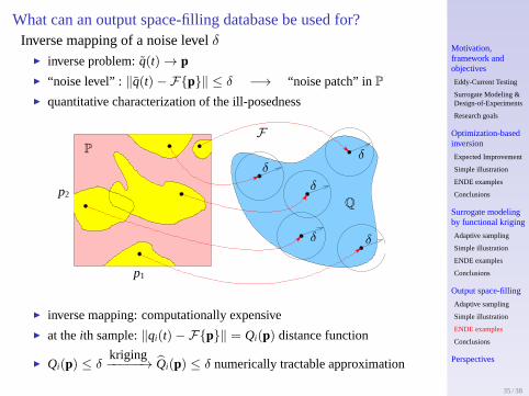
What can an output space-filling database be used for?Inverse mapping of a noise levelδ
inverse problem:q(t) → p “noise level” :‖q(t)−Fp‖ ≤ δ −→ “noise patch” inP
quantitative characterization of the ill-posedness
P
Q
δδ
δ
δ
δ
p1
p2
F
inverse mapping: computationally expensive
at theith sample:‖qi(t)−Fp‖ = Qi(p) distance function
Qi(p) ≤ δkriging−−−−−→ Qi(p) ≤ δ numerically tractable approximation
35 / 38

Motivation,framework andobjectives
Eddy-Current Testing
Surrogate Modeling &Design-of-Experiments
Research goals
Optimization-basedinversion
Expected Improvement
Simple illustration
ENDE examples
Conclusions
Surrogate modelingby functional kriging
Adaptive sampling
Simple illustration
ENDE examples
Conclusions
Output space-filling
Adaptive sampling
Simple illustration
ENDE examples
Conclusions
Perspectives
Illustration via ENDE examples II. : Noise level mappingThe 2-parameter example, output space-filling databases
9 samples,δ = 1 mΩ
L (mm)
D (
%)
1 1.5 2 2.5 3 3.5 4 4.5 5 5.5 6 6.5 7 7.5 8 8.5 9 9.5 105
10
15
20
25
30
35
40
45
50
55
60
65
70
75
80
85
90
9 samples,δ = 3 mΩ
L (mm)
D (
%)
1 1.5 2 2.5 3 3.5 4 4.5 5 5.5 6 6.5 7 7.5 8 8.5 9 9.5 105
10
15
20
25
30
35
40
45
50
55
60
65
70
75
80
85
90
36 samples,δ = 1 mΩ
L (mm)
D (
%)
1 1.5 2 2.5 3 3.5 4 4.5 5 5.5 6 6.5 7 7.5 8 8.5 9 9.5 105
10
15
20
25
30
35
40
45
50
55
60
65
70
75
80
85
90
36 samples,δ = 3 mΩ
L (mm)
D (
%)
1 1.5 2 2.5 3 3.5 4 4.5 5 5.5 6 6.5 7 7.5 8 8.5 9 9.5 105
10
15
20
25
30
35
40
45
50
55
60
65
70
75
80
85
90
36 / 38

Motivation,framework andobjectives
Eddy-Current Testing
Surrogate Modeling &Design-of-Experiments
Research goals
Optimization-basedinversion
Expected Improvement
Simple illustration
ENDE examples
Conclusions
Surrogate modelingby functional kriging
Adaptive sampling
Simple illustration
ENDE examples
Conclusions
Output space-filling
Adaptive sampling
Simple illustration
ENDE examples
Conclusions
Perspectives
Conclusions
Database generation
New adaptive DoE scheme: output space-filling
Samplingdistance functions−−−−−−−−−−−−−→ optimization task
Numerical burdenkriging−−−−−→ tractable algorithm
Inverse mapping
Tools involved in the database generation
Ill-posedness quantitatively accessible
Limitation: “Curse of Dimensionality”Perspectives
Other norms inQ
“Density estimation”→ inhomogeneous distance measure inP
Related articleS. Bilicz, M. Lambert and Sz. Gyimóthy“Kriging-based generation of optimal databases as forward and inverse surro-gate models,”Inverse Problems, 26(7), p. 074012, 2010.
37 / 38
Motivation,framework andobjectives
Eddy-Current Testing
Surrogate Modeling &Design-of-Experiments
Research goals
Optimization-basedinversion
Expected Improvement
Simple illustration
ENDE examples
Conclusions
Surrogate modelingby functional kriging
Adaptive sampling
Simple illustration
ENDE examples
Conclusions
Output space-filling
Adaptive sampling
Simple illustration
ENDE examples
Conclusions
Perspectives
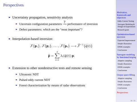
Perspectives
Uncertainty propagation, sensitivity analysis
Uncertain configuration parameters?−→ performance of inversion
Defect parameters: which are the “most important”?
Interpolation-based inversion:
Fp1, Fp2, . . . , Fpn −→ F−1q(t)
p =
n∑
i=1
λi(q(t)) pi
Extension to other nondestructive tests and remote sensing
Ultrasonic NDT
Pulsed eddy current NDT
Forest characterization by means of radar observations
38 / 38
Motivation,framework andobjectives
Eddy-Current Testing
Surrogate Modeling &Design-of-Experiments
Research goals
Optimization-basedinversion
Expected Improvement
Simple illustration
ENDE examples
Conclusions
Surrogate modelingby functional kriging
Adaptive sampling
Simple illustration
ENDE examples
Conclusions
Output space-filling
Adaptive sampling
Simple illustration
ENDE examples
Conclusions
Perspectives
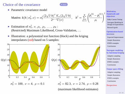
Choice of the covariance back
Parametric covariance model
Matérn:k(h |σ20, ν) = σ
20(2√ν h)ν Kν(2
√ν h)
2ν−1Γ(ν), h2 =
N∑k=1
(p(k)
i − p(k)j
ρi
)2
Estimation ofσ20, ν, ρ1, ρ2, . . . , ρN :
(Restricted) Maximum Likelihood, Cross-Validation, . . .
Illustration: a polynomial test function (black) and the kriginginterpolators (red) based on 5 samples:
0 0.2 0.4 0.6 0.8 10
5
10
15
20
25
30
p
Q(p)
σ20 = 100, ν = 4, ρ = 0.1
0 0.2 0.4 0.6 0.8 10
5
10
15
20
25
30
p
Q(p)
σ20 = 82.3, ν = 2.74, ρ = 0.28
(maximum likelihood estimates)39 / 38
Motivation,framework andobjectives
Eddy-Current Testing
Surrogate Modeling &Design-of-Experiments
Research goals
Optimization-basedinversion
Expected Improvement
Simple illustration
ENDE examples
Conclusions
Surrogate modelingby functional kriging
Adaptive sampling
Simple illustration
ENDE examples
Conclusions
Output space-filling
Adaptive sampling
Simple illustration
ENDE examples
Conclusions
Perspectives
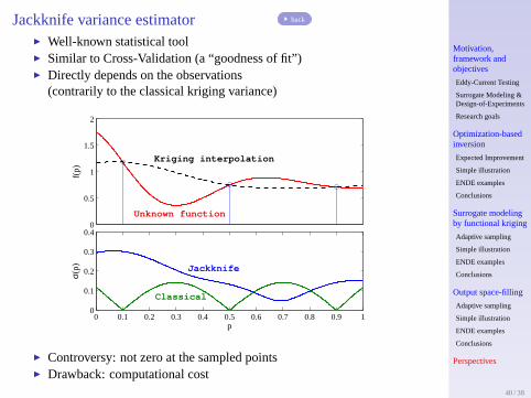
Jackknife variance estimator back
Well-known statistical tool Similar to Cross-Validation (a “goodness of fit”) Directly depends on the observations
(contrarily to the classical kriging variance)
0
0.5
1
1.5
2
f(p)
0 0.1 0.2 0.3 0.4 0.5 0.6 0.7 0.8 0.9 10
0.1
0.2
0.3
0.4
p
σ(p) Jackknife
Unknown function
Classical
Kriging interpolation
Controversy: not zero at the sampled points Drawback: computational cost
40 / 38
Motivation,framework andobjectives
Eddy-Current Testing
Surrogate Modeling &Design-of-Experiments
Research goals
Optimization-basedinversion
Expected Improvement
Simple illustration
ENDE examples
Conclusions
Surrogate modelingby functional kriging
Adaptive sampling
Simple illustration
ENDE examples
Conclusions
Output space-filling
Adaptive sampling
Simple illustration
ENDE examples
Conclusions
Perspectives
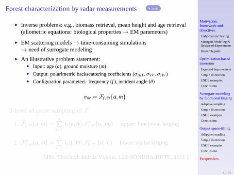
Forest characterization by radar measurementsback
Inverse problems: e.g., biomass retrieval, mean height and age retrieval(allometric equations: biological properties→ EM parameters)
EM scattering models→ time-consuming simulations→ need of surrogate modeling
An illustrative problem statement: Input: age (a), ground moisture (m) Output: polarimetric backscattering coefficients (σHH , σVV, σHV) Configuration parameters: frequency (f ), incident angle (θ)
σuv = Ff ,Θa,m
2-level adaptive sampling ofF
1. Ff ,Θa,m =n∑
i=1λi(a,m)FS
f ,Θai ,mi upper: functional kriging
2. FSf ,Θa,m =
k∑j=1
λj(f ,Θ)Ffj ,Θja,m lower: scalar kriging
[MSc. Thesis ofAndrásVASKÓ, L2S-SONDRA-BUTE, 2011.]
41 / 38

Motivation,framework andobjectives
Eddy-Current Testing
Surrogate Modeling &Design-of-Experiments
Research goals
Optimization-basedinversion
Expected Improvement
Simple illustration
ENDE examples
Conclusions
Surrogate modelingby functional kriging
Adaptive sampling
Simple illustration
ENDE examples
Conclusions
Output space-filling
Adaptive sampling
Simple illustration
ENDE examples
Conclusions
Perspectives
Age
Mois
ture
10 20 30 40 500.1
0.2
0.3
0.4
0.5
0.6
0.7
VV (σ = −28.2 dB)
Age
Mois
ture
10 20 30 40 500.1
0.2
0.3
0.4
0.5
0.6
0.7
VH (σ = −57.0 dB)
Age
Mois
ture
10 20 30 40 500.1
0.2
0.3
0.4
0.5
0.6
0.7
HH (σ = −20.6 dB)
Age
Mois
ture
10 20 30 40 500.1
0.2
0.3
0.4
0.5
0.6
0.7
Combined polarizations
Error maps for(a = 40, mv = 0.25), frequency bandwidth=[1000, 2000] MHz and incidenceangle range=[59, 61]. Black area: error less than 1 dB, dark grey: error between 1 dB and 2 dB,
light grey: between 2 dB and 3 dB. back 42 / 38