International Journal of Computer Applications (0975 – 8887)

Volume 101– No.5, September 2014

39

Application of Adaptive Neuro-Fuzzy Inference System

in High Strength Concrete

Behnam Vakhshouri

PhD candidate CBIR

University of Technology Sydney

Shami Nejadi Senior Lecturer

CBIR University of Technology Sydney

ABSTRACT

Abstract: Adaptive Neuro-Fuzzy Inference System is growing

to predict nonlinear behaviour of construction materials.

However due to wide variety of parameters in this type of

artificial intelligent machine, selecting the proper optimization

methods together with the best fitting membership functions

strongly affect the accuracy of prediction. In this study the non-

linear relation between splitting tensile strength and modulus of

elasticity with compressive strength of high strength concrete is

modelled and the effect of different effective parameters of

Adaptive Neuro-Fuzzy Inference System is investigated on

these models.

To specify the best arrangements of parameters in the System

to utilize in high strength concrete properties, different

combinations of optimization methods and membership

functions in the Sugeno system have been applied on more than

300 previously conducted experimental datasets. Both the grid

partition and sub-clustering methods have been applied to

models and compared to get the best combination of

parameters.

Keywords ANFIS, High strength concrete, Compressive strength,

Splitting tensile strength, Modulus of Elasticity

1. INTRODUCTION High Strength Concrete (HSC) is an especial type of concrete

to use in modern construction projects mostly in tall buildings

and towers to reduce the cumulative weight of the structure.

Application of HSC for tall buildings began in the 1970s,

primarily in the U.S.A. Use of HSC continues to spread,

particularly in the Far East and Middle East [1]. The definition

of high-strength concrete has changed over the years [2]. In the

1950s, concrete with a compressive strength (CS) of 5000 psi

(34 MPa) was considered HSC [1]. American Concrete

Institute (ACI), committee 363-92 selected 6000 psi (41 MPa)

as a lower strength limit for HSC [2]. Nowadays, due to

advances in concrete technology, it is possible to reach high

levels of CS and new classes of strength are introduced in

recent classifications in different design codes. While HSC in

ACI 363.2R has a specified CS of 8000 psi (55 MPa) or

greater, ACI 211.4R-08 specified CS equal to or less than 6000

psi (41 MPa) for normal strength concrete [3].

Accurate prediction of mechanical characteristics of hardened

concrete is almost the basic stage in design and evaluation of

reinforced concrete structures. In conjunction with the

traditional methods including destructive and non-destructive

tests and empirical relations to predict mechanical properties of

concrete, artificial intelligent based modelling methods have

been applied to simulate non-linear and complex behaviour of

various properties of construction materials in the recent years.

For ANFIS based soft sensor models, when

estimation/prediction accuracy is concerned, it is assumed that

both the data used to train the model and the testing data to

make estimations are free of errors (Klein and Rosin, 1999),

but rarely a dataset is without error (Jassar et al., 2009). Several

studies have investigated the effect of data errors on the outputs

of computer based models. Bansel et al. (1993) studied the

effect of errors in test data on predictions made by neural

network and linear regression models [4].

2. MATERIALS Almost all mechanical properties of concrete could be

estimated by the most important structural property of

concrete, CS. Selected mechanical properties of HSC in this

study include Splitting Tensile Strength (STS), Modulus of

Elasticity (MOE) and CS that are essential in all type of design

and evaluation of HSC structures. This study considers MOE

and STS as input and CS as output in ANFIS model. More than

100 sets of experimental studies in the last 15 years has been

collected from Giaccio and Zerbino(1998) [5], Jin-Kuen and

Sang-Hun (1999) [6], Shannag (2000) [7], Ajdukiewicz and

Kliszczewicz (2002) [8], Jin-Keun et al. (2004) [9],

Bissonnette et al. (2007) [10], Almeida et al. (2008) [11], Pablo

(2008) [12], Yin, J. et al. (2010) [13], K. M. Ng et al. (2010)

[14], Ozbay et al. (2011) [15], Parra et al. (2011) [16], Das and

Chatterjee (2012) [17], Ranaivomanana et al. (2013) [18].

To include wide range of experimental data in the model, lower

and upper limit of CS for HSC is selected 400 MPa and 1000

MPa respectively. Table 1, represents the range of collected

experimental mechanical properties for HSC in this study.

Table 1. Statistical values of mechanical properties of

HSC in this study

Mechanical

property

Min.

value

Max.

value Average

MOE (GPa) 21.3 49.9 38.37

STS (MPa) 2.28 7.4 4.33

CS (MPa) 40.4 98.8 57.01

Artificial intelligent model in ANFIS trains and compiles data

to establish a fuzzy logic between input and output values. To

validate the accuracy of the logic, it should be tested by some

other data from the experiments. To develop this model in

ANFIS, 240 datasets from the total of 305 datasets (79%) of

HSC mechanical properties, are considered as training data and

the remaining 21% as testing the data. To have similar

distribution of data in training and testing process, data is

classified in 6 equivalent groups of CS as indicated in table 21.

Then testing data have been selected based on percentage

weight of each group.

International Journal of Computer Applications (0975 – 8887)

Volume 101– No.5, September 2014

40

Table 2. Classification of data and number of selected testing data in each class

CS (MPa) 40–50 50-60 60–70 70–80 80-90 90-100

Percentage in all data 48 24 6 10 8 4

Number of testing data 10 5 1 2 2 1

3. ARTIFICIAL INTELLIGENT

BASED MODELS AND ANDIS To implement the fuzzy logic technique to a real application,

the following three steps are required:

1. Fuzzification: converts classical data or crisp data into

fuzzy data or Membership Functions (MFs)

2. Fuzzy Inference process: combines MFs with the control

rules to derive the fuzzy output

3. Defuzzification: returns a defuzzified value out, of a

MF positioned at associated variable value x using one of

several defuzzification strategies, according to the

argument type.

Fuzzy systems, Artificial Neural Network (ANN), adaptive

network-based inference, neuro-fuzzy and genetic fuzzy

systems are types of new generation of simulation and

modelling methods called artificial intelligent-based

modelling methods that is applicable in all fields of science. In

the field of civil and material engineering, it has been applied

to simulate non-linear and complex behaviour for various

properties of construction materials in recent years [21].

Fuzzy systems, is particularly useful in the engineering

applications where classical approaches fail or they are too

complicated to be used. ANFIS is a class of adaptive networks

which has the advantages of ANN and linguistic

interpretability of Fuzzy Inference Systems (FIS) [2, 19].

Application of ANFIS was first proposed by Jang (1993) [20]

used ANFIS to predict the CS of high performance

conventional concrete from fresh concrete properties.

Sadrmomtazi et al. (2013) [21] applied ANFIS analysis to

study the relation between CS of lightweight concrete and

mixing proportion.

3.1 Variables in ANFIS model ANFIS utilizes different variables including normalization

method, trial step quantity and various data classification

methods to achieve the minimum error between predicted

values and real data. Number and type of MF, type of output

MF, optimization method (hybrid or back propagation) and

the number of epochs are five important adjustments in

ANFIS to reach the most effective model with minimum

errors. This paper studies the effect of these adjustments and

their subdivisions in different combinations to develop new

ANFIS models and compare the results. For this purpose, all

possible combinations of these adjustments are applied to

unique sets of training and testing data.

3.2 Fuzzy rule-based inference system Mamdani and Tagaki-Sugeno fuzzy architectures are two

basic and well-known fuzzy rule-based inference systems in

artificial intelligent based modelling [22] that are mainly

different in the way to generate crisp output from the fuzzy

inputs [23] and linear or constant type of output MF [22].

Sugeno FIS uses weighted average to compute the crisp

output, while Mamdani FIS uses the technique of

defuzzification of a fuzzy output [23, 24].

Mamdani FIS has interpretable and intuitive nature of the rule

base and is widely used in decision support application and

studying human input [22], while Sugeno FIS is more

compact and computationally efficient representation and is

well suited to mathematical analysis.

Sugeno FIS lends itself to the use of optimization and

adaptive techniques for constructing fuzzy models and works

well with linear techniques (e.g., Proportional-Integral-

Derivative (PID) control). These adaptive techniques can be

used to customize the MFs so that the fuzzy system best

models the data. It also has guaranteed continuity of the

output surface [25]. Therefore considering these abilities and

advantages of Sugeno FIS especially in mathematical and

design systems, all models in this study are developed based

on the Sugeno FIS system.

3.3 Optimization methods ANFIS applies two optimization methods for FIS training.

First method is Hybrid Optimization Method (HOM) that is

default method in ANFIS and uses combination of least

squares and back-propagation to optimize the predicted

relations. The second method is known as back-propa (Back-

Propagation) Method (BPM). ANFIS performs the training

operation on the given real input and output data based on

error tolerance to create a training stopping criterion, which is

related to the error size. When the training data error remains

within this tolerance, the training will stop. Both type of

optimization methods are utilized in this study.

3.4 Membership functions Generally, fuzzification involves two processes; deriving the

MFs for input and output variables and representing them with

linguistic variables. Fuzzy algorithm categorises the

information entering a system and assigns values that

represent the degree of membership or degree of truth in those

categories. In fuzzy logic, degree of truth as an extension

of valuation is presented by MFs associated with terms that

appear in the antecedents or consequent of rules.

By applying MF in fuzzy system that is similar to

generalization of the indicator function in classical sets, a

fuzzy system allows members to have a smooth boundary

rather than classical sets.

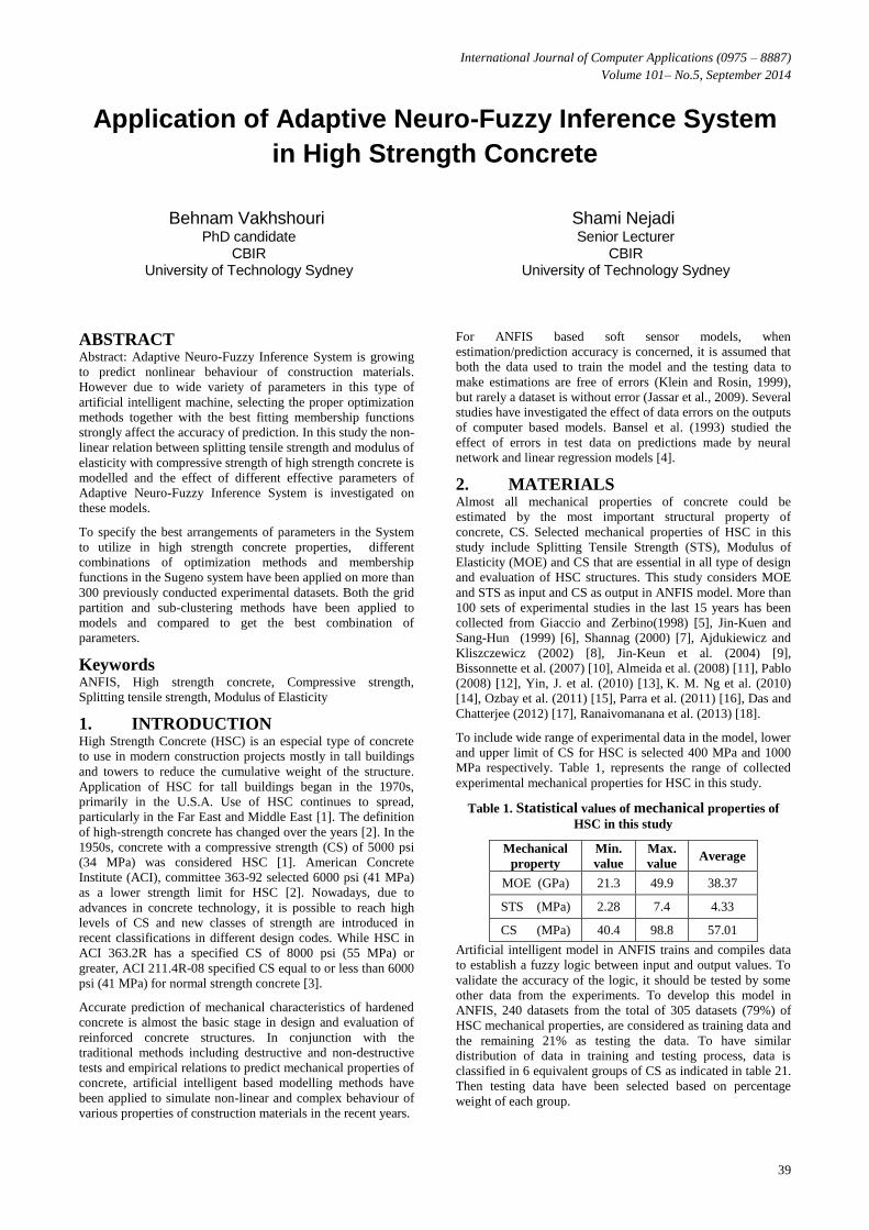
In practice, MFs can have multiple different types. Fig. 1

shows the mathematical model and distribution shape of 8

types of the MF including trimf, trapmf, gbellmf, gaussmf,

gauss2mf, pimf, dsigmf and psigmf that have been used in this

study. In addition there are other types of MF like S-curve,

and Z- shape that could be used in practical studies of fuzzy

systems. The MF choice is the subjective aspect of fuzzy

logic; it allows the desired values to be interpreted

appropriately. The exact type and shape of MF to apply in

each actual application depends on the purpose of the study

and parameters defining the uncertainty distribution function.

Relations between input uncertainty and MFs may be

estimated analytically [26]. For those systems that need

significant dynamic variation in a short period of time, a

triangular or trapezoidal waveform should be utilized. For

International Journal of Computer Applications (0975 – 8887)

Volume 101– No.5, September 2014

41

those system that need very high control accuracy, a Gaussian

or S-curve waveform may be selected. In the case of concrete

material properties [21] used the bell-shaped MF in the

ANFIS models.

3.5 Output membership function As mentioned before, there is just a constant MF available in

Mamdani FIS, but Sugeno architecture uses either linear or

constant type of output for MF. Therefore the Sugeno FIS

uses optimization techniques to find best parameters to fit data

instead of trying to do it heuristically. The present study

applies and compares both types of linear and constant output

MFs in combination with various optimization methods and

different numbers of epochs.

trimf- Triangular-

shaped MF

trapmf- Trapezoidal-

shaped MF

gbellmf- Generalized

bell-shaped MF

gaussmf – Gaussian

curve MF

gauss2mf- Gaussian

combination MF pimf- Π-shaped MF

dsigmf- Difference between

two sigmoidal functions MF

psigmf- product of

two sigmoidal MF

Fig. 1 – Shape and mathematical equations of utilized MF types

4. DEVELOPING ANFIS MODELS

IN MECHANICAL PROPERTIES OF

HSC Mechanical properties of HSC from different experimental

studies since 1998 have been collected. More than three

hundred datasets including STS, MOE and corresponding CS

at the age of 28 days are implemented in ANFIS neuro-fuzzy

system. CS is known as the most important characteristic of

concrete particularly in HSC and generally most of

mechanical properties of concrete like flexural strength, direct

tensile strength, STS and MOE are stated in terms of CS in

design codes, scientific and engineering references. In other

words, CS is a common characteristic between mechanical

properties of concrete. Consequently according to if-then rule

in Eq. (1), STS and MOE are considered as input data to give

CS as output.

Eq. (1)

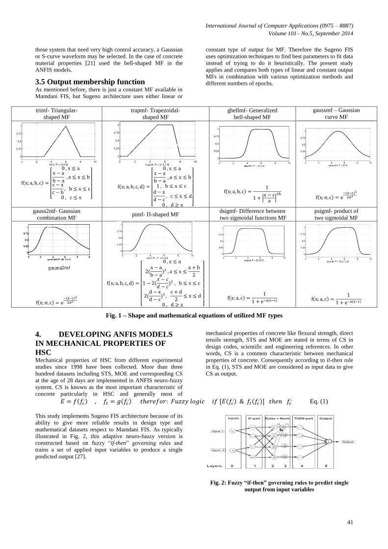
This study implements Sugeno FIS architecture because of its

ability to give more reliable results in design type and

mathematical datasets respect to Mamdani FIS. As typically

illustrated in Fig. 2, this adaptive neuro-fuuzy version is

constructed based on fuzzy “if-then” governing rules and

trains a set of applied input variables to produce a single

predicted output [27].

Fig. 2: Fuzzy “if-then” governing rules to predict single

output from input variables

International Journal of Computer Applications (0975 – 8887)

Volume 101– No.5, September 2014

42

Both hybrid and back-propagation neural network method of

optimization in six layers are integrated in the model to

remember experimental data pertaining to MOE and STS versus

28 days CS relationship of experimental investigations since

1998. The entire dataset of mechanical properties of HSC in

this study are 305 datasets that are referred to 240 datasets

(79%) as training data and 65 datasets (21%) as testing data.

After successful training, further testing data (not included in

training data) are applied to see how the ANFIS behaves for

known data. The testing data, evaluates the generalization

capability of the FIS at each epoch. In both training and

testing, ANFIS shows the error size which reflects the how

compatible the mapping function is [28]. The error size

computes the discrepancy between the network’s actual output

and a desired output.

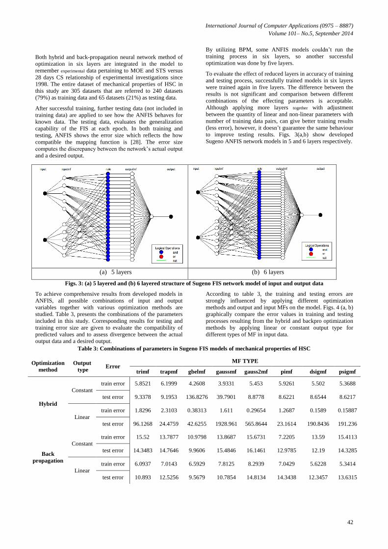
By utilizing BPM, some ANFIS models couldn’t run the

training process in six layers, so another successful

optimization was done by five layers.

To evaluate the effect of reduced layers in accuracy of training

and testing process, successfully trained models in six layers

were trained again in five layers. The difference between the

results is not significant and comparison between different

combinations of the effecting parameters is acceptable.

Although applying more layers together with adjustment

between the quantity of linear and non-linear parameters with

number of training data pairs, can give better training results

(less error), however, it doesn’t guarantee the same behaviour

to improve testing results. Figs. 3(a,b) show developed

Sugeno ANFIS network models in 5 and 6 layers respectively.

(a) 5 layers (b) 6 layers

Figs. 3: (a) 5 layered and (b) 6 layered structure of Sugeno FIS network model of input and output data

To achieve comprehensive results from developed models in

ANFIS, all possible combinations of input and output

variables together with various optimization methods are

studied. Table 3, presents the combinations of the parameters

included in this study. Corresponding results for testing and

training error size are given to evaluate the compatibility of

predicted values and to assess divergence between the actual

output data and a desired output.

According to table 3, the training and testing errors are

strongly influenced by applying different optimization

methods and output and input MFs on the model. Figs. 4 (a, b)

graphically compare the error values in training and testing

processes resulting from the hybrid and backpro optimization

methods by applying linear or constant output type for

different types of MF in input data.

Table 3: Combinations of parameters in Sugeno FIS models of mechanical properties of HSC

Optimization

method

Output

type Error

MF TYPE

trimf trapmf gbelmf gaussmf gauss2mf pimf dsigmf psigmf

Hybrid

Constant

train error 5.8521 6.1999 4.2608 3.9331 5.453 5.9261 5.502 5.3688

test error 9.3378 9.1953 136.8276 39.7901 8.8778 8.6221 8.6544 8.6217

Linear

train error 1.8296 2.3103 0.38313 1.611 0.29654 1.2687 0.1589 0.15887

test error 96.1268 24.4759 42.6255 1928.961 565.8644 23.1614 190.8436 191.236

Back

propagation

Constant train error 15.52 13.7877 10.9798 13.8687 15.6731 7.2205 13.59 15.4113

test error 14.3483 14.7646 9.9606 15.4846 16.1461 12.9785 12.19 14.3285

Linear

train error 6.0937 7.0143 6.5929 7.8125 8.2939 7.0429 5.6228 5.3414

test error 10.893 12.5256 9.5679 10.7854 14.8134 14.3438 12.3457 13.6315

International Journal of Computer Applications (0975 – 8887)

Volume 101– No.5, September 2014

43

It should be noted that unique values of actual input and

output data from the investigated mechanical properties of

HSC are implemented in all combinations, so comparing the

results is pretty reasonable and reliable. According to Fig.

4(a), the best compatible mapping function in training is

achieved from the HOM with linear output type and psigmf

input MF. While utilizing the BPM with constant output value

and gauss2mf input MF gives the biggest value of deviation.

In general, hybrid-linear provides more compatible mapping

than hybrid-constant, backpro-linear and backpro-constant

method which are in lower levels of compatibility in training

process.

According to Fig. 4(b), the best compatible mapping function

in testing is achieved from HOM with constant output type

and pimf input MF. While, utilizing the hybrid method with

linear output type and gaussmf input MF gives the largest

value of divergence. Generally, hybrid-constant, backpro-

linear and backpro-constant provide similar levels of

compatibility in mapping; conversely, hybrid-constant is

completely different and gives the worst predictions of testing.

Figs. 5 (a, b, c, d) shows the most and least compatibility

results for training and testing of developed models in ANFIS

as mentioned previously.

As general criterion in ANFIS models, the less testing error

gives more reliable predictions, but according to table 3, while

training and testing errors are not in the same level. It could be

mentioned that models with testing error close or up to two

times value of training error, are reasonable to be considered

for output values.

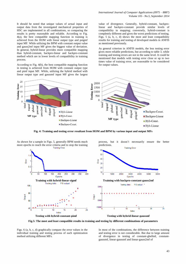
Fig. 4: Training and testing error resultant from HOM and BPM by various input and output MFs

As shown for a sample in Figs. 5, generally BPM needs much

more epochs to reach the error criteria and to stop the training

process, but it doesn’t necessarily ensure the better

predictions.

Training with hybrid-linear-sigmf Training with backpro-constant-gauss2mf

Testing with hybrid-constant-pimf Testing with hybrid-linear-gaussmf

Fig.5: The most and least compatible results in training and testing by different combinations of parameters

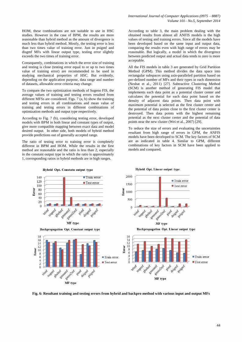
Figs. 6 (a, b, c, d) graphically compare the error values in the

individual training and testing process of each optimization

method utilizing different MFs.

In most of the combinations, the difference between training

and testing error is not considerable. But due to large amount

of divergence in testing of constant-gbellmf, constant-

gaussmf, linear-gaussmf and linear-gauss2mf of

International Journal of Computer Applications (0975 – 8887)

Volume 101– No.5, September 2014

44

HOM, these combinations are not suitable to use in HSC

studies. However in the case of BPM, the results are more

reasonable than hybrid method as the amount of divergence is

much less than hybrid method. Mostly, the testing error is less

than two times value of training error. Just in psigmf and

disgmf MFs with linear output type, testing error slightly

exceeds the two times of training error.

Consequently, combinations in which the error size of training

and testing is close (testing error equal to or up to two times

value of training error) are recommended to be used in

studying mechanical properties of HSC. But evidently,

depending on the application purpose, data range and number

of datasets, allowable error criteria may change.

To compare the two optimization methods of Sugeno FIS, the

average values of training and testing errors resulted from

different MFSs are considered. Figs. 7 (a, b) show the training

and testing errors in all combinations and mean value of

training and testing errors in different combinations of

optimization methods and output type respectively.

According to Fig. 7 (b), considering testing error, developed

models with BPM in both linear and constant types of output,

give more compatible mapping between exact data and model

desired output. In other side, both models of hybrid method

provide predictions out of generally accepted range.

The ratio of testing error to training error is completely

different in BPM and HOM. While the results in the first

method are reasonable and the ratio is less than 2, especially

in the constant output type in which the ratio is approximately

1, corresponding ratios in hybrid methods are in high ranges.

According to table 3, the main problem dealing with the

obtained results from almost all ANFIS models is the high

values of testing and training errors. Since all the models have

been developed based on the same input and output data,

comparing the results even with high range of errors may be

reasonable. But logically, a model in which the divergence

between predicted output and actual data tends to zero is more

acceptable.

All the FIS models in table 3 are generated by Grid Partition

Method (GPM). This method divides the data space into

rectangular subspaces using axis-paralleled partition based on

pre-defined number of MFs and their types in each dimension

(Neshat et al., 2011) [27]. Subtractive Clustering Method

(SCM) is another method of generating FIS model that

implements each data point as a potential cluster center and

calculates the potential for each data point based on the

density of adjacent data points. Then data point with

maximum potential is selected as the first cluster center and

the potential of data points close to the first cluster center is

destroyed. Then data points with the highest remaining

potential as the next cluster center and the potential of data

points near the new cluster (Wei et al., 2007) [29].

To reduce the size of errors and evaluating the uncertainties

resultant from high range of errors in GPM, the ANFIS

models have been developed to SCM. The key factors of SCM

are as indicated in table 4. Similar to GPM, different

combinations of key factors in SCM have been applied to

models and compared.

Fig. 6: Resultant training and testing errors from hybrid and backpro method with various input and output MFs

International Journal of Computer Applications (0975 – 8887)

Volume 101– No.5, September 2014

45

(a) (b)

Fig. 7: a) Comparative diagram of individual exact training and testing errors in different MFs and b) comparative diagram

between mean values of all MFs in two types of optimization

Default values of IR, SF, AR and RR in ANFIS are 0.5, 1.25,

0.5 and 0.15 respectively. Different combinations of these

factors give completely different training and testing errors.

To evaluate the effect of each factor in training and testing of

implemented data for HSC properties, keeping constant the

values of the 3 corresponding factors, various values of each

individual factor were studied. For example, to evaluate the

effect of IR, different models were developed with changing

value of IR with constant values of SF, AR and RR. Figs. 8 (a,

b, c and d) show the effect of each factor in training and

testing errors of ANFIS models.

Table 4: Key factors of Subtractive Clustering method to

generate FIS models

Factor Function

Influential

Radius (IR) Directly affect the clustering result

Squash factor

(SF)

Used to multiple the given radii values to

squash the potential of outlying points to

be considered as part of that cluster

Accept Ratio

(AR)

Sets the potential as a fraction of the

potential of the fiirst cluster center and

above which a data point will be accepted

as a cluster center

Reject Ratio

(RR)

Sets the potential as a fraction of the first

cluster center and below which a data

point will be rejected as a cluster center.

-5

0

5

10

15

20

25

30

35

40

0 0.2 0.4 0.6 0.8 1

Err

or

Range of Influence

Train error

Test error

0

5

10

15

20

25

30

0 0.2 0.4 0.6 0.8 1 1.2 1.4 1.6

Err

or

Squash Factor

Train error

Test error

(a) (b)

0

2

4

6

8

10

12

14

0 0.2 0.4 0.6 0.8 1

Err

or

Accept Ratio

Train error

Test error

0

2

4

6

8

10

0 0.2 0.4 0.6 0.8 1

Err

or

Reject Ratio

Train error

Test error

(c) (d)

Figs. 8: Effect of a) IR, b) SF, c) AR and d) RR in compatibility of developed models with actual data

International Journal of Computer Applications (0975 – 8887)

Volume 101– No.5, September 2014

46

According to Figs. 8 (a, b, c and d), RI and SF have similar

effects on developed models, while AR and RR behave

similarly. Considering default values of ANFIS for SF, AR

and RR, the error range of training and testing has sever

fluctuations for RI <0.5 and tend to be stable after IR>0.5.

The least error (best compatibility) for testing could be

achieved by IR around 0.5, however the best compatibility of

training error is issued from IR about zero. Other diagrams

could give similar conclusions for training and testing error

size of models. Advantage of these individual diagrams of

factors is to enable designer to choose best combinations for

different applications and goals. However, to have

comprehensive comparison database, different combinations

of these factors are included in models and the results are

presented in table 5. Fig. 9 compares the results from table 5.

According to Fig.9, the difference in error sizes from various

combinations of coefficients in table 5 is not considerable and

majority of errors are less than 10. In combination 3 with

equal coefficients, BPM gives the maximum error size both in

testing and training process and according to Fig. 8a, gives a

high level of testing error in combination 13. While hybrid

method gives the maximum testing error size in combination

10 with default values of ANFIS.

5. RECOMMENDATIONS AND

CONCLUSIONS Adaptive Neuro-Fuzzy Inference System (ANFIS) models

was developed utilizing more than 300 datasets of previously

conducted experiments on mechanical properties of HSC to

investigated the predict CS from STS and MOE.

Comparing the Mamdani and Sugeno FIS architectures in

ANFIS, the Sugeno FIS was selected to apply on models.

Both methods of grid partition and sub-clustering were

applied to generate the models. All possible arrangements of

different types of optimization methods, input and output MFs

in grid partition method have been considered. Individual

effect of each factor in sub-clustering method investigated and

30 combinations of these factors to achieve the best

compatibility between actual and predicted values of output

data have been performed.

Default values in ANFIS for both grid partition and sub-

clustering don’t guarantee the accuracy of predicted output

values.

In general, hybrid-linear provides more compatible mapping

than hybrid-constant, backpro-linear and backpro-constant

method which are in lower levels of compatibility in training

process.

- Considering mean value of error of all combinations in

training and testing, both models of hybrid method provide

predictions out of generally accepted range.

RI and SF have similar effects on developed models, while

AR and RR behave similarly.

The combinations in which the error size of testing is close to

training error, (up to twice value) are recommended to be used

in studying mechanical properties of HSC. However,

regarding the study goal, parameters include, range and

number of datasets, allowable error criteria may change.

Table 5: Different combinations of SCM factors to achieve the best compatibility between actual and predicated output data

RI SF AR RR Train error Test error Train error Test error

1 0.1 0.1 0.1 0.1 0.079057 10.7871 1.3441 11.139

2 0.2 0.2 0.2 0.2 0.37837 65.63 171.9405 125.4327

3 0.3 0.3 0.3 0.3 2.385 38.717 31513 15787

4 0.5 0.5 0.5 0.5 6.8151 8.5082 6.5166 8.3276

5 0.50 1.25 0.50 0.15 7.9993 8.5222 8.2224 8.13

6 0.40 1.25 0.50 0.15 5.7485 59.4575 6.143 24.47

7 0.30 1.25 0.50 0.15 5.1829 10.4982 5.4437 6.9088

8 0.20 1.25 0.50 0.15 4.362 23.3443 4.6183 8.8283

9 0.10 1.25 0.50 0.15 0.079057 10.5453 1.049 12.7126

10 0.50 1.25 0.50 0.10 6.891 594575 7.5618 8.4724

11 0.40 1.25 0.50 0.10 5.3585 7.4856 5.4594 16.0323

12 0.30 1.25 0.50 0.10 5.1829 10.4982 5.3895 7.1057

13 0.20 1.25 0.50 0.10 2.8404 32.2165 5719.1888 5719.0301

14 0.10 1.25 0.50 0.10 0.079057 10.5453 0.98461 12.7644

15 0.50 0.85 0.50 0.15 5.7935 7.2018 6.6061 8.9627

16 0.50 0.90 0.50 0.15 5.7935 7.2018 6.6061 8.9627

17 0.4 1 0.4 0.1 4.6893 8.8516 5.1066 7.9642

18 0.3 1 0.3 0.05 3.7816 21.6565 27.0156 35.2149

19 0.2 0.9 0.2 0.05 0.96361 26.8212 1.1062 19.8803

20 0.6 1.15 0.1 0.1 6.8567 7.7563 7.0954 9.1198

21 0.8 0.8 0.2 0.2 7.1996 7.4159 8.1147 8.262

22 0.2 0.2 0.8 0.8 7.2225 7.3259 6.4234 7.1726

23 0.50 1.25 0.40 0.15 7.9993 8.5222 8.1967 8.2423

24 0.50 1.25 0.30 0.15 7.9993 8.5222 8.1967 8.2423

25 0.50 1.25 0.20 0.15 7.9993 8.5222 8.1967 8.2423

26 0.50 1.25 0.10 0.15 5.7141 7.3396 6.7377 8.8877

27 0.50 1.15 0.50 0.15 6.8289 7.1216 7.5115 8.1572

28 0.50 1.05 0.50 0.15 6.6835 7.5287 7.5284 8.7259

29 0.50 1.00 0.50 0.15 5.7935 7.2018 6.5912 9.0539

30 0.50 0.95 0.50 0.15 5.7935 7.2018 6.5842 9.1069

sub clustering coefficents Hybrid method Backpro method

International Journal of Computer Applications (0975 – 8887)

Volume 101– No.5, September 2014

47

0

1000

2000

3000

4000

5000

6000

7000

8000

9000

10000

1 2 3 4 5 6 7 8 9

10

11

12

13

14

15

16

17

18

19

20

21

22

23

24

25

26

27

28

29

30E

rro

r si

ze i

n d

iffe

ren

t a

rra

ngem

ents

Arrangements of Sub-clustering factors in table 5

Hybrid method Train error

Hybrid method Test error

Backpro method Train error

Backpro method Test error

Fig. 9: Comparing the error size of training and testing in different combinations of factors in Sub-Clustering

method

6. REFERENCES [1] ACI-363-10, Report on High-Strength Concrete,

Reported by ACI Committee 363, 1st printing, March

2010

[2] Ghosh S.K. (2004), High strength concrete in U.S codes

and standards, XIV Congreso Nacional de Ingeniería

Estructural, Acapulco, Gro

[3] ACI 211.4R-08, (2008), Guide for Selecting Proportions

for High-Strength Concrete Using Portland Cement and

Other Cementitious Materials”, Reported by ACI

Committee 211

[4] S. Jassar, Z. Liao, Ashrae, L. Zhao (2009), Impact of

Data Quality on Predictive Accuracy of ANFIS based

Soft Sensor Models, Proceedings of the World Congress

on Engineering and Computer Science 2009 Vol II

WCECS 2009, October 20-22, San Francisco, USA

[5] Giaccio G. and Zerbino R. (1998), Failure Mechanism of

Concrete, Advanced Cement Based Materials, Volume

7(2), March 1998, pp. 41–48

[6] Kim Jin-Kuen and Han Sang-Hun (1999), Mechanical

Properties of Self-Flowing Concrete, ACI Special

Publication, vol. 172 pp. 637-652

[7] Shannag M.J. (2000), High strength concrete containing

natural pozzolan and silica fume, Cement & Concrete

Composites, vol. 22, pp.399-406

[8] Ajdukiewicz A. and Kliszczewicz A.(2002), Influence of

recycled aggregates on mechanical properties of

HS/HPC, Cement & Concrete Composites 24, pp.269–

279

[9] Kim J. Keun; Lee Y., Yi, S. Tae (2004), Fracture

characteristics of concrete at early ages, Cement and

Concrete Research vol. 34 issue 3. pp. 507-519

[10] Bissonnette B., Pigeon M. and Vaysburd Alexander M.

(2007), Tensile Creep of Concrete: Study of Its

Sensitivity to Basic Parameters, ACI Materials Journal,

V. 104, No. 4, July-August

[11] Almeida Filho F. M., Barragan B. E., Casas J. R., and

Eldebs A. L. H. C. (2008), Variability of the bond and

mechanical properties of self-compacting concrete,

IBRACON structures and materials journal, Volume 1,

Number 1,pp. 31–57

[12] Angel Perez J. Pablo (2008), Effect of slag cement on

drying shrinkage of concrete, thesis submitted in

conformity with the requirements for the degree of

Master of Applied Science, September 2008, University

of Toronto.

[13] Yin, J., Chi, Y., Gong, S., and Zou, W. (2010), Research

and Application of Recycled Aggregate Concrete, Paving

Materials and Pavement Analysis, GeoShanghai 2010

International Conference, Shanghai, Chinapp. June 3-5,

pp:162-168, 10.1061/41104(377)19

[14] Ng K. M., Tam C. M. and Tam V. W. Y. (2010),

Studying the production process and mechanical

properties of reactive powder concrete: a Hong Kong

study, Magazine of Concrete Research, Volume 62, Issue

9, pp. 647 –654

[15] Ozbay E., Gesoglu M., Guneyisi E. (2011), Transport

properties based multi-objective mix proportioning

optimization of high performance concretes, Materials

and Structures 44:139–154

[16] Parra C., Valcuende M., Gomez F. (2011), Splitting

tensile strength and modulus of elasticity of self-

compacting concrete, Construction and Building

Materials 25, 201–207

[17] Das D., Chatterjee A. (2012), A comparison of hardened

properties of fly-ash-based self-compacting concrete and

normally compacted concrete under different curing

conditions, Magazine of Concrete Research, Volume 64,

Issue 2 Volume 64, Issue 2, , pages 129 – 141

[18] Ranaivomanana N., Multon S., Turatsinze A. (2013),

Tensile, compressive and flexural basic creep of concrete

at different stress levels, Cement and Concrete Research

52 1–10

[19] Joelianto E., Rahmat B. (2008), Adaptive Neuro Fuzzy

Inference System (ANFIS) with Error Backpropagation

Algorithm using Mapping Function, International journal

of artificial intelligence, Volume 1, Number A08

[20] Ozel C., (2011), prediction of compressive strength of

concrete from volume ratio and Bingham parameters

International Journal of Computer Applications (0975 – 8887)

Volume 101– No.5, September 2014

48

using adaptive neuro-fuzzy inference system(Anfis) and

data mining, Int. J. Physical sciences, Vol. 6(31),

pp.7078-7094

[21] Sadrmomtazi, J. Sobhani, M.A. Mirgozar

(2013),Modeling compressive strength of EPS

lightweight concrete using regression, neural network

and ANFIS, Construction and Building Materials 42, pp.

205–216

[22] Chai Y., Jia L. and Zhang Z. (2009), Mamdani Model

based Adaptive Neural Fuzzy Inference System and its

Application, International Journal of Information and

Mathematical Sciences, 5:1

[23] Kaur A., Kaur Amrit (2012), Comparison of Mamdani-

Type and Sugeno-Type Fuzzy Inference Systems for Air

Conditioning System, International Journal of Soft

Computing and Engineering (IJSCE), Volume-2, Issue-2

[24] Naderloo L., Alimardani R., Omid M., Sarmadian F.,

Javadikia P., Torabi M. Y., Alimardani F. (2012),

Application of ANFIS to predict crop yield based on

different energy inputs, Measurement 45, 1406–1413

[25] Takagi T. and Sugeno M. (1985), Fuzzy identification of

systems and its applications to modeling and control,

IEEE Trans. Syst., Man, Cybern, 15:116–132

[26] Duch W. (2004), Uncertainty of data, fuzzy membership

functions, and multi-layer perceptrons, IEEE Transaction

on neural networks, vol. XX, No. YY, 2004-1

[27] Neshat M., Adeli A., Masoumi A., sargolzae M., (2011),

A Comparative Study on ANFIS and Fuzzy Expert

System Models for Concrete Mix Design, IJCSI

International Journal of Computer Science Issues, Vol. 8,

Issue 3, No. 2

[28] Rezazadeh shirdar M., Nilashi M., Bagherifard K.,

Ibrahim O., Izman S., Moradifard H., Jamshidi N., Mehdi

Barisamy (2011),Application of ANFIS system in

prediction of machining parameter, Journal of

Theoretical and Applied Information Technology, Vol.

33 No.1

[29] Wei M., Bai B., Sung A. H., Liu Q., Wang J., Cather M.

E. (2007), Predicting injection profiles using ANFIS,

Information Sciences 177,pp. 4445–4461

IJCATM : www.ijcaonline.org