Appliance Electrical Consumption Modelling at Scaleusing Smart Meter Data

D.M. Murraya,∗, L. Stankovica, V. Stankovica, N.D. Espinoza-Oriasb

aDepartment of Electronic and Electrical Engineering, University of Strathclyde, 204George St., Glasgow, United Kingdom

bNestle Research Center, Nestec S.A., Vers-Chez-Les-Blanc, 1000 Lausanne 26, Switzerland

Abstract

The food industry is one of the world’s largest contributors to carbon emissions,

due to energy consumption throughout the food life cycle. This paper is focused

on the residential consumption phase of the food life cycle assessment (LCA),

i.e., energy consumption during home cooking. Specifically, while much effort

has been placed on improving appliance energy efficiency, appliance models used

in various applications, including the food LCA, are not updated regularly. This

process is hindered by the fact that the cooking appliance models are either very

cumbersome, requiring knowledge of parameters which are difficult to obtain or

dependent on manufacturers’ data which do not always reflect variable cooking

behaviour of the general public. This paper proposes a methodology for gen-

erating accurate appliance models from energy consumption data, obtained by

smart meters that are becoming widely available worldwide, without detailed

knowledge of additional parameters such as food being prepared, mass of food,

etc. Furthermore, the proposed models, due to the nature of smart meter data,

are built incorporating actual usage patterns reflecting specific cooking practice.

We validate our results from large, geographically spread energy datasets and

demonstrate, as a case study, the impact of up-to-date models in the consump-

tion phase of food LCA.

∗Corresponding authorEmail addresses: david.murray@strath.ac.uk (D.M. Murray ),

lina.stankovic@strath.ac.uk (L. Stankovic), vladimir.stankovic@strath.ac.uk(V. Stankovic), NamyDaniela.EspinozaOrias@rdls.nestle.com (N.D. Espinoza-Orias)

Preprint submitted to Cleaner Production March 15, 2018

Keywords: Appliance modelling, Appliance usage, Energy savings, Life cycle

assessment

1. Introduction

The food industry worldwide accounts for a significant fraction of carbon

emissions. For example, in the United Kingdom (UK) alone, the food industry

is responsible for about 14% of the energy consumption of the entire industry

sector, equivalent to 7 million tonnes of carbon emissions per year [1]. The food

Life Cycle Assessment (LCA) estimates material and energy input and output

at all stages of the food product’s life cycle − from acquisition of raw materials,

production, processing, and packaging, to consumer use, and waste/recycling.

For many food products, including ready meals, domestic cooking takes up a

significant fraction of the total energy consumption of the product’s LCA [2], [3],

[4]. Although the energy consumption of domestic cooking in developed coun-

tries has decreased by 31% from 1991 to 2008 [3], mainly due to improved energy

efficiency of cooking appliances, cooking and beverage preparation in domestic

settings still consume a substantial amount of energy, or approximately 7Mega

Joule (MJ)/Kilogram (kg) [5, 6]. For example, according to [7], in the United

States, domestic cooking accounts for 8-16% (equivalent to 6.9×108 Giga Joule

per year) of the total national annual energy consumption [8]. Similarly, the

report on Energy Consumption and Efficiency Trends in the European Union

(EU) [9] estimates the energy consumption for ovens and hobs in private house-

holds in the EU-27 to be approximately 60 Tera-Watt hour (TWh) and states

that for cooking appliances, there is still potential for energy savings. The situ-

ation is worse in many developing countries, where cooking consumes up to 90%

of the overall residential energy consumption [10, 11], and it is mainly based on

non-renewable energy.

Jungbluth [12] provides an early inventory of data for cooking at home using

various appliances, so that food LCA studies can accurately quantify the food

preparation stage. Sensitivity analysis of efficiency (ratio of energy input to

2

energy output) shows that the type of vessels used, type of electrical appliance

used (grill, oven, microwave oven, cast iron plate, induction stove), and the

preparation method, have a large influence, resulting in the conclusion that there

are large differences between efficiencies. Lakshmi et al. [13] tested different

methods to cook rice in a microwave with different power levels, including the

influence of soaking the rice prior to cooking. It was concluded that an electric

rice-cooker is more energy efficient despite a longer cooking time compared to

the microwave, but microwave cooking is as energy efficient as using a pressure

cooker. A similar study on energy efficiency of cooking rice is presented in Das

et al. [14], but only an electric rice cooker and a pressure cooker are tested.

Zufia and Arana [15] carried out the LCA of an industrially cooked dish,

namely cooked tuna with tomato sauce, to assess the environmental impact of

the production and distribution. However, the electricity consumed at home by

a microwave for heating the ready meal is not considered. Calderon et al. [16]

model the microwave consumption using its power rating, and focus on LCA

of a canned ready meal, a stew product based on cooked pulses and pork meat

cuts, highlighting subsystems with the highest environmental loads, concluding

that 11% of the total energy consumption in the product life cycle is attributed

to the domestic level. More recently, in [17], environmental burdens of the same

dish at four production scales is considered, including canned food (reheated at

home), the restaurant (cooked and heated in a traditional way and served), and

the home-made dish with electricity consumption at household level estimated

from electrical appliance specifications.

Oberascher et al. [18] highlight the variability of behaviour of consumers in

using electrical appliances at the domestic level and provides empirical data on

electricity consumption for a number of cooking processes, including heating

water, baking potatoes and boiling eggs, concluding that the energy consump-

tion of the microwave for heating water is lower than stove with a pot with and

without a lid, but higher than kettle. Experiments conducted by Vattenfall [19]

show that using the most energy efficient appliance in the kitchen for a specific

cooking job is undoubtedly an effective way of lowering energy consumption.

3

However, Fechner shows differences of up to 50% in energy consumption when

six chefs all cooked the same meal with the same equipment (cited as per [20]),

which agrees with the findings of DeMerchant [21]. Kemna [22] expects no fur-

ther energy-saving potential possible for electric ovens from 2010 to 2020 from a

purely technical design point of view; however, with a change to more sustain-

able consumer behaviour, the additional potential for energy savings is expected

to be about 10% [22].

The literature survey above demonstrates a clear need to capture the effect of

different cooking styles, and consequently variable appliance usage, and explore

the impact of the consumer phase, particularly at domestic level, in food LCA

studies. This requires wider studies that can only be enabled via accurate

and scalable models for computing the energy aspect of end-user cooking at

home, and not relying on appliance manufacturer’s specifications to estimate

the consumption.

To this end, in [4], general models for quantifying energy consumption related

to the food preparation in private households are proposed, including frying,

boiling, oven roasting and microwave cooking. This is achieved via appliance

load modelling, through exhaustive tests in laboratory conditions using different

appliances and cooking settings. However, the models generated require a large

number of variables to be known, such as type of food, its mass, the evaporation

mass of food, which is not possible at scale. Similarly, the modelling of the

combined oven in a restaurant setting, proposed recently in [23], also includes a

large number of parameters which are not approachable at scale. Industrial scale

applications already have a number of studies conducted, which model industrial

versions of household appliances, such as modelling the cooking properties of

industrial bread ovens [24]. These, however, are very specific to the industry in

question and therefore non transferable methodologies are applied.

This paper is inspired by some of the work done over a decade ago [4], and

the appliance modelling performed, albeit in a different context, e.g., [25] where

lines of best fit are applied for each setting of washing machines and [26] that use

online survey, in-home study and laboratory experiments to assess the energy

4

consumption of refrigerators. This paper proposes a methodology for generating

general appliance models in a scalable manner to quantify energy consumption

related to the usage of cooking appliances at domestic level. Specifically, our

research hypothesis is that only smart meter data, comprising active power mea-

surements with at least 60 second sampling in a similar format to the UK Smart

Metering Equipment Technical Specifications v2(SMETS2) [27], is sufficient for

building accurate major cooking appliance models. To prove our hypothesis,

the paper draws upon load profiling, appliance mining and user activities assess-

ment methodologies related to energy demand literature [28, 29]. For example,

in [28], smart meter data is used to assess energy efficiency and sustainability

of electric kettle usage. In [29], energy demand of different energy consuming

domestic activities such as cooking and laundering is quantified. Load profiles

of 11 major domestic appliances is studied in [30] showing that the majority of

cooking load profiles are single state even when there may be large variation

during the operation of the appliance.

While the proposed methodology is generic to all cooking appliances, in this

paper, for ease of understanding, the methodology is illustrated on two electric

cooking appliances with wide ownership in most countries, namely the electric

oven and microwave. According to [31], almost 70% of households with ovens

in England have electric ovens and just under 30% have gas ovens. Thus, in

our study we chose to focus only on electrical appliances as they have a market

dominance and the eventual move away from fossil fuels should increase the

ownership of electrical appliances.

The appliance models proposed have a two-fold advantage over existing mod-

els: (i) models reflect current, more energy efficient and wider capacity appli-

ances and (ii) models are not reliant on parameters that are difficult to estimate

by non-specialists in large field studies. The proposed models are validated with

existing literature, as well as on large electrical measurements datasets where

electrical consumption of the two appliances in question was recorded. Further-

more, in order to demonstrate applicability and impact on food LCA, a case

study is provided where figures for the microwave oven and electric oven are

5

calculated for frozen ready meals and compared with recent LCA for the same

food [32].

Note that smart meter data is now abundant for many countries allowing

for many different applications such as non-intrusive load monitoring (NILM)

(see [33] and [29] and references therein), consumption forecasting, demand re-

sponse, load scheduling and energy saving feedback. Currently, there are many

smart meter datasets openly accessible from different countries, providing do-

mestic consumption patterns for geographically specific locations [34–37]. The

proposed models can facilitate usage of these existing datasets to study sustain-

ability in geographically spread households, e.g., by quantifying energy wastage

and efficiencies due to different cooking appliances and practices.

The paper is organised as follows: Section 2 briefly reviews relevant appli-

ance energy consumption models, Section 3 provides an overview of the proposed

methodology and details of the field study carried out to build the appliance

models, Section 4 describes the proposed models for oven and microwave, Sec-

tion 5 shows the results of validating the proposed models on large-scale datasets

and Section 7 presents a food LCA case study showing the viability of the pro-

posed models. Section 8 concludes the work and highlights opportunities for

future work.

2. Existing Energy Consumption Models

In this section, existing models for the microwave and electric oven are re-

viewed for quantifying energy consumption related to food preparation in the

domestic sector. Both appliances have some functionality overlap, but use com-

pletely different heating methods.

The state-of-the-art microwave (MW) energy consumption model [4] requires

knowledge of the food being cooked as well as water content, infeasible to collect

at scale. It is given by:

EMW [MJ ] = (mfood × Telev × cp + (mevap × eew))/etotmw, (1)

6

where the following parameters are required:

mfood = mass of product (in grams [g])

telev = difference in food temperature (in Celsius degrees [oC])

cp = heat capacity of the food product [MJ/(g×oC)]

mevap = mass of water evaporated [g]

eew = 2.26×10−3 [MJ / g water evaporated]

etotmw = esupport × etrans × emagn × emwcoup

esupport = 0.95 (efficiency for fan & lamp & controls)

etrans = 0.86 (efficiency for transformation)

emagn = 0.73 (efficiency for the magnetron)

emwcoup = 0.57 + 3.8×10−4 ×mfood (for 200 < mfood < 1000g)

emwcoup = 0.95(for mfood > 1000g).

A similar microwave model is used in [13]. We note that other studies, briefly

reviewed in Section 1, such as [18], [17], [16], [13], rely on heuristic measurements

in laboratory conditions, or focus on preparation of particular dishes, or rely on

power rating of the appliances and cooking recipes with the risky, and sometimes

wrong assumption, that they will be followed.

The model for oven, validated in [4] using 23-59 litre ovens and data supplied

by The Swedish Consumer Agency (http://www.konsumentverket.se) which had

oven volumes ranging between 18-65 litres, is given by:

EOV EN (MJ) = Ehu × V × T + Emt × V × T × t

+ Ehp ×mtot ×∆T + 2.26×10−3 ×mwevap

+ 3.34×10−4 ×mfrozen.

(2)

The model requires the following input parameters:

7

Ehu = 2.0 ∗ 10−4

Energy for heating one litre of oven volume. [(MJ/(litre×oC))]

V = volume of the oven in [litres]

T = temperature the oven is heated to (−20oC start temp)[oC]

Emt = 4.2 ∗ 10−6

Energy for maintaining a certain oven temperature in

one litre for one minute [MJ/(litre×minutes)]

t = time for cooking (excluding preheating) [minutes]

mtot = mass of product [g]

mwevap = mass of water evaporated [g]

mfrozen = mass of the product if frozen [g]

ehp = heat capacity of the food product [MJ/(kg×oC)].

Obviously, many of these parameters cannot be easily collected during a field

study, since collecting some of these parameters requires information or devices

not widely available, such as scales, thermometer, heat capacity of foods etc.

Furthermore, the collection is often timely, cumbersome, expensive and cannot

be expected to be conducted at scale by untrained volunteers in field studies.

Thus, to the best of our knowledge, scalable appliance consumption models,

suitable to estimate accurate energy consumption that captures varied cooking

styles in a longitudinal study, is missing.

3. Methodology

Our aim is to provide models which can be easily applied to numerous ex-

isting smart meter energy datasets (see [35] for partial list) or used in large

longitudinal consumer and energy studies, where information may be lacking

with regards to specialised knowledge such as cooking settings, food tempera-

ture, appliance makes and models. Our research hypothesis is that by using only

8

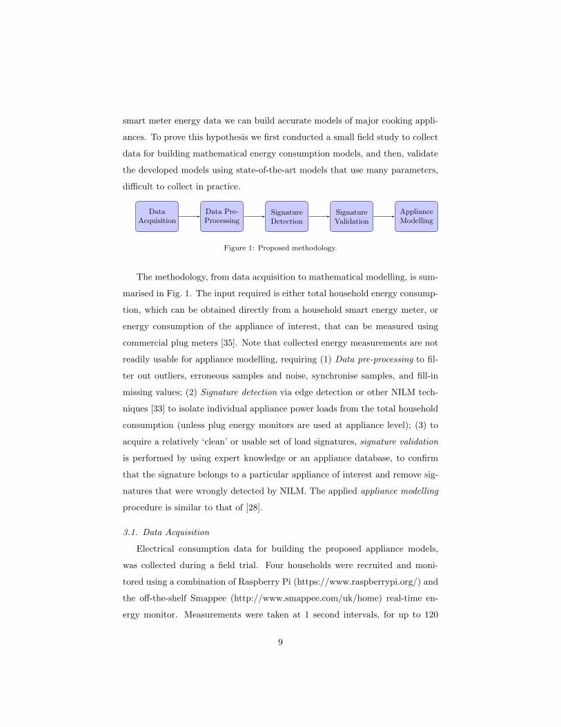
smart meter energy data we can build accurate models of major cooking appli-

ances. To prove this hypothesis we first conducted a small field study to collect

data for building mathematical energy consumption models, and then, validate

the developed models using state-of-the-art models that use many parameters,

difficult to collect in practice.

DataAcquisition

Data Pre-Processing

SignatureDetection

SignatureValidation

ApplianceModelling

Figure 1: Proposed methodology.

The methodology, from data acquisition to mathematical modelling, is sum-

marised in Fig. 1. The input required is either total household energy consump-

tion, which can be obtained directly from a household smart energy meter, or

energy consumption of the appliance of interest, that can be measured using

commercial plug meters [35]. Note that collected energy measurements are not

readily usable for appliance modelling, requiring (1) Data pre-processing to fil-

ter out outliers, erroneous samples and noise, synchronise samples, and fill-in

missing values; (2) Signature detection via edge detection or other NILM tech-

niques [33] to isolate individual appliance power loads from the total household

consumption (unless plug energy monitors are used at appliance level); (3) to

acquire a relatively ‘clean’ or usable set of load signatures, signature validation

is performed by using expert knowledge or an appliance database, to confirm

that the signature belongs to a particular appliance of interest and remove sig-

natures that were wrongly detected by NILM. The applied appliance modelling

procedure is similar to that of [28].

3.1. Data Acquisition

Electrical consumption data for building the proposed appliance models,

was collected during a field trial. Four households were recruited and moni-

tored using a combination of Raspberry Pi (https://www.raspberrypi.org/) and

the off-the-shelf Smappee (http://www.smappee.com/uk/home) real-time en-

ergy monitor. Measurements were taken at 1 second intervals, for up to 120

9

days. At the beginning of the study, all four households filled an Appliance

Usage Survey containing information about appliance ownership and general

patterns of appliance usage, again for the purposes of signature validation. The

survey confirmed that all houses owned a microwave and all but one was likely

to use it daily; ovens are most likely to be used in the afternoon and evenings.

In addition, for the purposes of validation, time diaries were also kept by

household participants, including recording the start time of each appliance use

along with settings of the appliance in use. Recorded start times in time diaries

are in general accurate to around 1-2 minutes of the actual usage time. It was

found that the recording of the recipe or type of food prepared using an electrical

appliance did not affect the energy consumption in a significant way and thus

did not affect the appliance consumption models.

3.2. Data Pre-processing

The first step is making sure the measurements are suitable for use by fil-

tering out outliers and erroneous measurements, including spikes, following a

similar methodology to [35].

The second step is synchronisation of readings. Raw data generally does

not have a uniform sampling rate and therefore isolating appliance signatures

becomes more complex when varying time frequencies are involved. Re-sampling

timestamped data to one second intervals helps to achieve this uniformity; each

sample is rounded to the nearest second (in this case removing the millisecond

component). Once this is completed, forward filling using a previous sample fills

any gaps which have arisen. Forward filling however should be limited (in our

case we chose 2 seconds) to avoid skewing electrical signatures. These methods

are generic regardless of the data source.

3.3. Signature Detection and Validation

Smart meters measure only the household’s total energy consumption. To

use smart meter data for appliance load modelling, it is necessary to isolate

10

appliance usage, which is commonly done via NILM [33]. For this study, we

develop a simple, supervised, edge-detection based method given in Algorithm 1.

The input to the algorithm are smart meter active power readings col-

lected at time t, powt in Watts (W), which are used to calculate edges, as

∆powt = powt − powt−1, defined as difference in power value between sequen-

tial timestamps. An edge could be either a rising or a falling edge: a RisingEdge

is a positive change in power (e.g., when an appliance is switched on or goes to

a high consuming state) and a FallingEdge is a negative change in power (e.g.,

an appliance going to a low consuming state or is switched off).

The appliance metadata are data gathered from time diaries and individual

appliance monitoring (IAM); these include instantaneous maximum and mini-

mum observed power draw for the appliance of interest (powmin and powmax)

and time durations (durmin and durmax), and the number of states. Since the

power draw of the appliances of interest oscillates between high power state

(e.g., heating state) and low power state (maintaining the heat), to avoid pick-

ing up low power state as switching off the appliance (that is, as a FallingEdge),

we also estimate switching time as the time between an appliance going to a low

power state (where it may appear to be off) before returning to a high powered

state.

After all candidate RisingEdge and FallingEdge are detected, each RisingEdge

is matched with the closest in time FallingEdge if the time duration between

these two edges is within the acceptable limits, that is, between durmin and

durmax, minimum and maximum appliance operation time duration observed

from the Appliance metadata. Next, by comparing the time difference between

the rising and falling edges with switching time, a check is performed to ensure

that the FallingEdge is not due to appliance transiting to a low power state.

11

Input : Data(Time(t), Power(powt)), Appliance Metadata

Load Appliance Metadata:

Minimum & Maximum Time Duration (durmin; durmax) ;

Minimum & Maximum Power (powmin; powmax);

switching time;

Output: Time Duration tsecs & Energy Consumption Eapp

RisingEdge = , FallingEdge = , Edges = , Signature = ;

for (t, powt) in Data do

Calculate: ∆powt = powt − powt−1 ;

Store: RisingEdge(t, |∆powt|) IF powmin ≤ ∆powt ≤ powmax;

Store: FallingEdge(t, |∆powt|) IF -powmax ≤ ∆powt ≤ -powmin;

end

i=0;

for tRE in RisingEdge do

for tFE in FallingEdge do

if durmin ≤ tFE − tRE ≤ durmax then

Store: Edges(tRE ,∆powRE), (tFE ,∆powFE);

Calculate:

Eappi= (∆powRE + ∆powFE)× (tFE − tRE)/(2× 106) ;

i = i + 1 ;

end

end

end

for (tRE , tFE) in Edges do

if |tFE − tRE+1| ≤ switching time then

(tFE ,∆powFE) = (tFE+1,∆powFE+1) ;

Calculate: EappFE= EappFE

+ EappFE+1;

if tFE+1 − tRE ≤ durmax then

Store: Signature(tFE ,∆powFE , tRE ,∆powRE , EappFE) ;

end

end

end

for (tFE , tRE) in Signature do

Calculate Duration as: tsecs[sec]=tFE-tRE ;

end

Algorithm 1: Signature Detection Pseudocode. The MatLab code

is available at https://github.com/David-Murray/MatLab-Appliance_

EdgeDetection.

12

The proposed edge detection algorithm is limited by multiple simultaneous

appliance uses and appliances with similar-valued consumption and duration.

More sophisticated NILM methods can be used to provide higher disaggregation

accuracy [33, 34, 38].

Algorithm 1 is run for each appliance of interest separately, and it returns

the time duration and energy consumption of each detected appliance-of-interest

use. To ensure that none of these detected uses comes from another appliance

with similar load, or with multiple appliances being switched on/off at the

same time, for each paired output Rising/Falling edge, we perform check with

time diary or IAM measurements, if available, or validate it against known

appliance signatures, e.g., [39], to check if they fall within a valid range of

values (e.g., similar consumption, duration, time of day). This is done to ensure

that incorrectly disaggregated signatures are not used for the modelling stage.

All correct, labelled appliance signatures, namely the duration tsecs[sec] and

energy consumption (Eapp[MJ ]) per use, are then fed to the Appliance Mod-

elling stage in Section 4 where app refers to the appliance being modelled, e.g.,

MW for microwave.

4. Appliance Modelling

In this section, we perform curve fitting on the processed and cleaned energy

measurements, namely time duration and energy consumption, to construct gen-

eralised models of appliance consumption based only on information gathered

from smart energy meters as described in Section 3 and are widely available in

numerous existing smart meter datasets that have been made public (see Table

1 in [35]). Note that other parameters such as temperature, food weight etc.,

which are difficult to gather during a large-scale longitudinal energy and con-

sumer studies, are excluded. Resulting mathematical models for the microwave

and the oven are presented next.

13

4.1. Microwave Consumption Model

The microwave’s power consumption over time is pulsed as microwaves are

typically run at either 100% power, or variations on this at 20% intervals (20, 40,

60, 80%). To develop a model, the time duration (tsecs) and energy consump-

tion (EMW ) values were obtained using the Signature Detection algorithm (i.e.,

Algorithm 1) as explained in Section 3.3. The other two parameters used in the

model are: powerwatts, that is, the rated magnetron power of the microwave,

obtained from the appliance manual or information labels of the respective mi-

crowaves, which is fixed for each microwave; and settingpercentage, which denotes

the power setting of the microwave (e.g., 60% of powerwatts), as set by the con-

sumer per run and, for the purpose of model development, was obtained from

time diaries.

Following curve fitting on the output of Section 3.3, which isolated 584 valid

microwave signatures, the following mathematical linear model for the consumed

energy is obtained:

EMW (MJ) = (0.0010899× tsecs) + (powerwatts × 5.8681×10−6). (3)

It should be noted that the above microwave model is limited by the availabil-

ity of consumption data, and thus it is inadvertently biased towards the tested

microwaves, which ranged between 700W and 900W. Reduced power band set-

tings, e.g., 80% of 700W (560W), will be estimated well while, 60% of 700W

will be over estimated. To reduce errors of predicting lower powered microwaves

and, as such give a better overall range, 700W uses were weighted appropriately

to help improve model predictions. This resulted in a more accurate quadratic

microwave model, given in equation below:

14

EMW (MJ)Quadratic = (0.0015893× powerwatts)

+ (−1.4823× settingpercentage)

+ (0.0001032× tsecs)

+ (0.0020663× (powerwatts × settingpercentage))

+ (−9.9386e− 08× (powerwatts × tsecs))

+ (0.0012324× (settingpercentage × tsecs))

+ (−2.237e− 06× (power2watts))

+ (0.018915× (setting2percentage))

+ (−5.1134e− 07× (t2secs)).

(4)

Compared to the previous linear model, this quadratic model incorporates

the power percentage setting (settingpercentage) of the microwave as a variable

(e.g., 60%, 80%). Note that, in contrast to previous models (see Section 2),

our model predicts the amount of consumed energy EMW based purely on the

duration tsecs, power rating powerWatts (which is a fixed parameter for each

microwave, e.g., 900, 800W, etc.), and settingpercentage of the microwave, which

can be easily recorded. Alternatively, the model can predict microwave setting,

based on the measured EMW and tsecs, that is, purely from the Algorithm 1’s

output.

We first validate our proposed model visually by comparing the predicted

energy consumption values from the model with actual energy consumption

values, as shown in Figure 2. Six distinct power settings were used in the time

diaries gathered, resulting in powerwatts × settingpercentage consumption bands

of 900W, 800W, 700W, 560W, 420W, and 280W of which, there were 28, 6,

148, 185, 208, 9 uses, respectively. The normalised root mean squared error

(NRMSE), calculated using Eq(7), for these 6 settings is 0.44, 0.15, 0.002, 0.04,

0.05, and 0.04, respectively.

It can be seen from Figure 2, that the Predictions from the quadratic model

show a very good fit with the actual measurements for all power settings, includ-

15

ing the 900W setting that shows the highest NRMSE. Therefore, we conclude

that the NRMSE between actual measurements and predicted values from the

model of the microwave of around 0.5 is acceptable.

0 50 100 150 200 250 300

Duration

(Seconds)

0

0.05

0.1

0.15

0.2

0.25

0.3

0.35

0.4

Co

nsu

mp

tio

n

(MJ)

Microwave Consumption vs Duration

900W

800W

700W

560W

420W

280W

Predictions

Figure 2: Detected microwave consumptions and predicted values using the proposed

quadratic model Eq. 4.

Furthermore, Table 1 shows how our model output compares to that of the

state of the art [4], described in Section 2. As in [4], the ratio, measured as the

predicted energy usage from the model divided by the measured energy usage,

is used for assessing the accuracy, i.e., the results closer to 1 indicate better

prediction. The better performing method is highlighted in green.

Microwave Power Duration (mins/secs) Son. Model Prediction Our Model Our Model (Quad) Son. Measured Ratio Son. Ratio Our Ratio Our (Quad)

750 3/5 0.23 0.21 0.23 0.22 1.05 0.95 1.09

750 3/5 0.20 0.21 0.23 0.22 0.91 0.95 1.09

800 2/53 0.25 0.19 0.23 0.22 1.14 0.86 1.05

700 3/18 0.25 0.22 0.23 0.22 1.14 1 1.05

750 4/30 0.37 0.30 0.32 0.32 1.16 0.94 1.00

750 4/30 0.28 0.30 0.32 0.32 0.88 0.94 1.00

800 3/0 0.28 0.20 0.23 0.22 1.27 0.90 1.09

700 4/0 0.28 0.27 0.27 0.25 1.12 1.08 1.08

Table 1: Comparison of the model prediction of Sonesson [4] (abbreviated to Son.) and our

proposed linear Eq. 3 & quadratic model Eq. 4 using the values recorded by [4] given in [MJ].

We can see that the proposed quadratic model is more accurate than the

proposed linear model and benchmark model of [4]. This confirms that knowl-

16

edge of the food being prepared does not impact the consumption phase of the

microwave in a significant manner.

In [16], it claimed that an 800W rated microwave at 100% for approx 8 min-

utes consumes 0.1kWh (0.36 MJ). Using our linear model the same microwave

would be expected to consume 0.1394kWh (0.5 MJ), and our quadratic model

would be consuming 0.1919kWh (0.69 MJ).

4.2. Oven Consumption Model

Oven-baking is still one of the most used cooking practices in Europe, with

electric ovens present in most homes [4, 23]. The oven operates in two stages: (i)

preheating/restoring heat, when the oven typically draws a constant power load,

and (ii) maintaining heat. The set temperature, type and amount of food being

baked, affects only the time the oven will be in each of the two states. Within

this section, to build a model, the time duration (tsecs) and energy consumption

(EOven) were obtained from the edge detection algorithm (i.e., Algorithm 1) as

described in Section 3.3; the set temperature (tempOven) of the oven has been

obtained from time diaries, or if this is not available, estimated based on the

initial preheating duration, which is close to linear for each oven.

Most cooking recipes require the oven to be pre-heated to a set temperature.

During this phase, the oven door is usually kept shut meaning that the time to

reach temperature will be linear with the assumption that the oven is in good

working order and condition. The cooking phase may consist of door openings

as food is introduced and later checked or taken out. When the door is opened

the oven will lose temperature and require another heating stage to return to the

set temperature. Different oven settings produce different signatures; however,

they still retain the general heating/maintenance cycle with adjusted timings.

In our models we assume that the door is not opened frequently or unnecessarily

and that only one dish is added for the cooking stage. Note that the model is

limited by the available oven data, that is, we expect that the model will not

accurately represent very large (≥ 80 litres) or very small ovens (≤ 50 litres).

In developing a scalable model for the oven load, we start from the Sonesson

17

model given by Eq.(2) and attempt to remove dependency of the model on

parameters that are difficult to acquire.

First, using the data collected from smart meters (see Subsection 3.1) we

estimate two static parameters of Eq.(2) - Ehu and Emt. As the values reported

in [4] were set back in 2003, our obtained estimates differ from Eq.(2) due to

the newer and more energy efficient oven designs. This situation further moti-

vates our proposal for appliance modelling methodologies that can be updated

regularly, without significant effort and cost.

In our field study, the 58-litre oven is the oldest and worst performing from an

energy point of view. The average energy values given by Eq.(2) for V = 58 litre

oven, for energy needed for heating and maintaining the heat, respectively, are

Ehu = 2.0×10−4 [MJ/(litre×oC)] and Emt = 4.3×10−6 [MJ/(litre×minutes)].

Our experiments show that this value should be lowered to around

1.1055×10−4[MJ/(litre×oC)] for Ehu. Our recommendation is to increase

slightly the Emt value from Eq.( 2) to 1.7288×10−5[MJ/(litre×minutes)] due

to the increase in the size of oven cavities. Table 2 summarises the mean and

variance of the values obtained from our models from the detailed field study of

two ovens, where the combined average is the recommended value for Ehu and

Emt.

Volume (Litre)Ehu Emt

Mean Variance Mean Variance

58 1.2905×10−04 1.6243×10−10 2.1575×10−05 2.3426×10−11

74 8.0806×10−05 1.6753×10−10 1.0398×10−05 1.0288×10−11

Combined Avg. 1.1055×10−04 1.7288×10−05

Table 2: Experimentally obtained values for the energy needed for heating and maintaining

the heat, for the two ovens in the study.

Table 2 is an update to the model of [4] described in Section 2; however

the large number of variables that need to be known hamper using the model

18

in large-scale studies. Instead, we propose the following scalable model, if the

oven volume is unknown:

EOven[MJ ] = (0.0037372×tempOven[oC]) + (0.0011084×tsecs[s]). (5)

The difference in the volume of the oven causes variations resulting in an

NRMSE between predicted and actual values of 0.25, as calculated by Eq.(7).

We conclude that volume is important for estimating power consumption, espe-

cially with the current large variation in oven volumes on the market. A revised

model that incorporates time duration, set temperature and oven volume is

given by the following equation:

EOven[MJ ] =

(−0.064859×V [Litre])

+ (0.028626×tempOven[oC])

+ (0.00094777×tsecs[sec]).

(6)

With the addition of the Volume (V ) component, Eq. (6) has a reduced

NRMSE of 0.19 when compared to Eq.(5). Fig. 3 shows the validation results for

the energy consumption vs. operation time for the two ovens, this time showing

a much better agreement between the predicted values from the revised model

from Eq.(6) and the actual measured values. Therefore, we define an acceptable

value for NRMSE between actual measurements and predicted values from the

model of the oven to be around 0.3.

19

0 500 1000 1500 2000 2500 3000 3500 4000 4500 5000

Duration

(Seconds)

0

1

2

3

4

5

6

7C

on

su

mp

tio

n

(MJ)

Oven Consumption vs Prediction Models

Measured

Model Incl. Volume

Model Excl. Volume

Figure 3: Oven Total Energy Consumption against time: actual (black circles) vs. Predicted

(red diamond & blue circle).

5. Model validation using publicly available datasets

To further validate our models at scale and investigate the effect of variability

of consumer behaviour, as reported in Oberascher et al. [18], on the proposed ap-

pliance models, we use data from several publicly available datasets, including:

(a) REFIT dataset [35], that comprises aggregate readings and individual appli-

ance power consumption from 20 UK households taken over a period of 2 years

where householders were going about their normal day-to-day routines under no

test conditions; (b) eco dataset from Switzerland [36]; (c) REDD dataset from

the United States [40]. The datasets were chosen to validate against geographic

variability in appliance type ownership and patterns of use, and experiments

were conducted over hundreds of uses for statistical accuracy.

We use NRMSE as a measure of the error. NRMSE was chosen as large errors

are more heavily weighted than Mean Absolute Error (MAE); this is desirable,

as a lower NRMSE shows that the model is less prone to inaccurate estima-

tions and therefore when performing LCA or yearly consumption estimates the

model is proven to be a reliable guide. The NRMSE captures the error in the

models predicted consumption against the actual measured consumption, and

20

was calculated as:

NRMSE =1

1N

∑Ni=1 Eappmeasuredi

√∑Ni=1(Eappmodeli

− Eappmeasuredi)2

N(7)

where Eappmodeliand Eappmeasuredi

denote the energy consumption estimated by

the model and measured, during the i-th use, respectively, of the appliance in

question (microwave or oven), and N is the number of appliance uses detected

in the dataset.

5.1. Microwave

Table 3 shows the NRMSE results for microwave from the REFIT dataset

where microwave model, i.e., its power rating, is known. Note that, in the

REFIT dataset, the readings were collected at 6-8 sec interval. At the time of the

REFIT study, the measurements were made with a less accurate electricity meter

than the one used to build our model, and this resulted in higher acquisition

noise and synchronization issues. Out of 20 households monitored, the make

and model number of 7 microwaves were collected during the REFIT study,

which means that the output power, i.e., powerwatt, for these seven microwaves

was known. Table 4 shows the equivalent results for eco and REDD datasets,

where the make and model of the microwaves are unknown.

The small NRMSE values for all microwaves in both Tables 3 and 4 (below

the acceptable boundary of 0.5) confirm that the proposed microwave model

of Eq. (4) accurately estimates the energy consumption without any knowledge

about the type of food being cooked or the food temperature, and also that

the proposed model is accurate even with variable consumer behaviour across

different households and countries. NRMSE was only large for Houses 9 and 17

due to high level of noise in the dataset and many loads running in parallel.

21

REFIT House Known Power [W] Uses NRMSE

House 3 1000 611 0.28

House 4 700 1395 0.35

House 5 1000 2442 0.47

House 8 1000 1429 0.27

House 9 700 146 0.53

House 17 850 715 0.55

House 20 800 755 0.36

Table 3: Model (Eq. 4) NRMSE when predicted for 7 microwaves from the REFIT dataset,

where output power is known. House numbers correspond to the numbers in the REFIT

dataset. Known Power refers to the known power rating of the microwave, i.e., powerwatt is

known.

House Estimated Power [W] Uses NRMSE

REDD-H1 700 278 0.25

REDD-H2 900 46 0.34

REDD-H3 900 46 0.27

ECO-H4 700 812 0.31

ECO-H5 700 59 0.33

Table 4: Model (Eq. 4) NRMSE when predicted for microwaves from eco and REDD datasets.

House numbers correspond to the numbers in the REDD and Eco datasets. Estimated Power

refers to the guessed power rating of the appliance, i.e., powerwatt is assumed based on the

measurements.

22

0 50 100 150 200 250 300

Duration

(Seconds)

0

0.05

0.1

0.15

0.2

0.25

0.3

0.35

0.4

0.45C

on

su

mp

tio

n

(MJ)

Prediction (Quadratic Model) for REDD House 1

RDDH1

700W

700W@40%

Figure 4: Prediction of microwave from REDD House 1, where powerWatts and

settingpercentage is unknown. The consumed power is predicted using the quadratic model

Eq. (4). The actual readings are denoted by RDDH1.

Fig. 4 shows energy consumption vs. duration for REDD House 1 - mea-

sured values (in black) and predicted consumption using the proposed quadratic

model (Eq. 4). It can be seen that the model estimates the load measurements

accurately, despite the fact that power rating powerwatt is unknown. Assum-

ing a 700W power setting (taken from Table 4) at 100% and 40% (280W) the

NRMSE for the house drops from 0.25 to 0.17.

5.2. Oven

The proposed oven model is validated using the REDD dataset, which in-

cludes an oven monitored at plug level (no disaggregation needed) and the RE-

FIT dataset, where oven uses were extracted from the aggregate data using the

methodology described in Section 3.3. Fig. 5 shows the energy consumption vs.

time duration, for House 1 from the REDD dataset and Houses 1 and 10 from

the REFIT dataset. Oven make and model for both datasets are unknown, as is

the target temperature. Consumption measurements obtained from three ovens

with 53 uses using the aforementioned datasets are plotted using red markers.

The proposed model, Eq. (6), showing prediction consumption values, is plot-

ted for the following parameters: volumes (Litre) of 56, 65, and 74, and target

23

temperatures of 160oC and 180oC.

Figure 5: Oven predictions using the proposed model and reference model [12] for House 1

from REDD (RDD) dataset and Houses 1 and 10 from REFIT (RFT) dataset.

It can be observed that the actual measurements (RDDH1, RFTH10, RFTH1)

fall within the predicted consumption using our model for four different oven

volume and temperature combinations (where values are specified by Vol for

Volume given in Litres and Temp for Temperature given in oC). Visually Fig. 5

confirms that the models are accurate and that knowledge of the type of food

being prepared does not impact on the accuracy of the model. The model is

especially accurate when the duration is up to 45 mins. A lower accuracy of the

model for durations greater than an hour is probably due to a lower tempera-

ture setting used, or the oven door being opened too many times, resulting in

an NRMSE of 0.2868, 0.5208, 0.3260, and 0.2873, for the four cases shown in

Fig. 5, respectively, because the temperature and volume for the oven measure-

ments are unknown so cannot be matched to each usage scenario. We also show

how the actual measurements compare with those predicted by the reference

model of [12] from 1997, shown as dotted lines in Fig. 5. As expected, the latter

model (Jungbluth) overestimates the actual consumption, predicting it in the

range 0.132 MJ/min to 0.234 MJ/min. We can conclude that ovens now come

with better efficiencies and that models need to be updated regularly to reflect

24

contemporary ownership.

6. Limitations of the study and threats to the validity of results

In this section, we summarise two limitations of the proposed models, namely

detection of appliance signatures from the smart meter aggregate load intro-

duced in Section 3.3, and availability of appliance models used for model gen-

eration in Sections 4.1 and 4.2.

Algorithm 1, proposed in Section 3.3, uses edge detection to isolate usages of

appliances of interest (i.e., oven and microwave). The edge detection algorithm

is limited by multiple simultaneous appliance uses and appliances with similar-

valued consumption and duration. Appliance uses in these circumstances are

excluded from modelling due to uncertainty. More sophisticated NILM methods

can be used to provide higher disaggregation accuracy [33, 34, 38]. Alternatively,

individual appliance power measurement sensors can be used to directly measure

power consumption of the appliances of interest.

Secondly, limitations arise from the availability of appliance models, namely

microwaves and ovens in our case. Indeed, the microwave model, proposed in

Section 4.1, is limited by the availability of consumption data, and thus it is

inadvertently biased towards the microwaves used in the study, which ranged

between 700W and 900W. Therefore, the accuracy of the model is expected to

be lower for microwaves rated at greater than 1000W. Similarly, the oven model,

proposed in Section 4.2, is limited by the available ovens used in the study, that

is, we expect that the model will not accurately represent very large (≥ 80 litres)

or very small ovens (≤ 50 litres). At the time of the study, we endeavoured to

include most commonly available microwave power ratings and oven volumes in

the market. Models proposed in the study are validated on publicly available,

recent (to reflect contemporary appliance ownership) UK, Swiss and USA smart

meter datasets in Section 5 resulting in very good accuracy. The oven model is

especially accurate when the duration of use is up to 45 minutes.

25

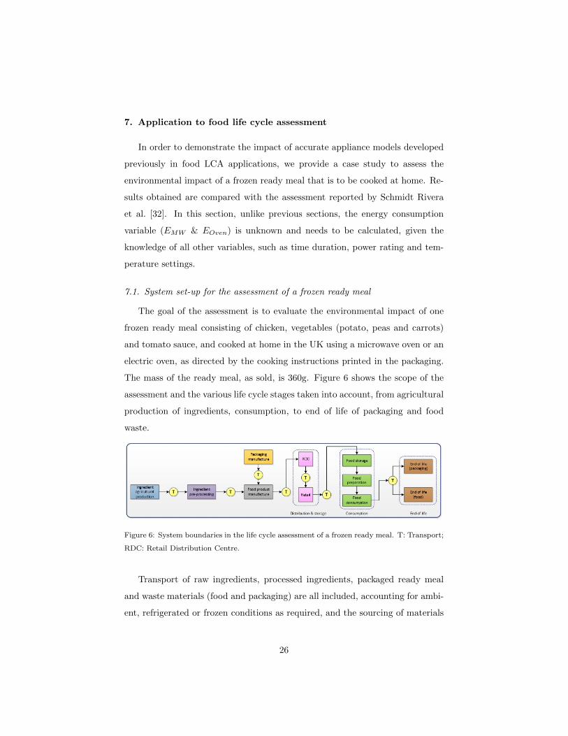
7. Application to food life cycle assessment

In order to demonstrate the impact of accurate appliance models developed

previously in food LCA applications, we provide a case study to assess the

environmental impact of a frozen ready meal that is to be cooked at home. Re-

sults obtained are compared with the assessment reported by Schmidt Rivera

et al. [32]. In this section, unlike previous sections, the energy consumption

variable (EMW & EOven) is unknown and needs to be calculated, given the

knowledge of all other variables, such as time duration, power rating and tem-

perature settings.

7.1. System set-up for the assessment of a frozen ready meal

The goal of the assessment is to evaluate the environmental impact of one

frozen ready meal consisting of chicken, vegetables (potato, peas and carrots)

and tomato sauce, and cooked at home in the UK using a microwave oven or an

electric oven, as directed by the cooking instructions printed in the packaging.

The mass of the ready meal, as sold, is 360g. Figure 6 shows the scope of the

assessment and the various life cycle stages taken into account, from agricultural

production of ingredients, consumption, to end of life of packaging and food

waste.

Figure 6: System boundaries in the life cycle assessment of a frozen ready meal. T: Transport;

RDC: Retail Distribution Centre.

Transport of raw ingredients, processed ingredients, packaged ready meal

and waste materials (food and packaging) are all included, accounting for ambi-

ent, refrigerated or frozen conditions as required, and the sourcing of materials

26

(local, regional or imported). Primary, secondary and tertiary packaging of

the ready meal is included. Food waste along the value chain as well as post-

consumer waste is also taken into account.

In particular, cooking of the frozen ready meal is modelled as detailed in

Table 5, for six scenarios considered in this assessment. The home cooking

stage is modelled using three different sources of data: the appliance models

proposed in the paper, the World Food LCA Database (WFLDB) [41], and the

energy consumption models by a microwave oven and an electric oven developed

by Jungbluth [12] and used in [32].

Scenario Appliance Cooking Parameters Appliance model Energy Consumption [MJ] Source

1 Electric oven 200oC for 40min 0.183 MJ/min(Heat up + maintenance) 7.32 [12][32]

2 Electric oven 200oC for 40min, Oven volume: 67Litre Eq. (6) 3.65 This paper

3 Electric oven 10min preheat, 200oC for 40min Oven calculator of WFLDB (Heat up + maintenance) 2.16 + 1.44 = 3.6 [41]

4 Microwave oven 9min 0.0435 MJ/min 1.41 [12][32]

5 Microwave oven 800W for 9min Eq. (4) 0.56 This paper

6 Microwave oven 800W for 9min 0.088 MJ/min (standby & heating) 0.79 [41]

Table 5: Description of home cooking of one frozen ready meal. Six different scenarios are

considered: 3 with electric oven and 3 with microwave.

The precise details of the inputs to the life cycle inventory of the study

are detailed in [32] and were reproduced here (quantities, distances, cooking

instructions, etc.). Background life cycle inventories (LCI), as shown in Table

6, are taken from publicly available databases: ecoinvent v.3.3 (SCLCI, 2016)

and World Food LCA Database [41], and further detailed in [32]. The energy

sources are regionalised for the elements considered key in this study, namely

pre-processing of vegetables in the UK, manufacturing of ready meals in the UK,

and use of the microwave oven in the UK. The other inputs contain electricity

at either a European level or at global level. Two environmental impact indi-

cators are evaluated: (1) greenhouse gas emissions [42] and (2) abiotic resource

depletion - fossil fuels (CML, 2014) [43], which provide a suitable overview of

the environmental impacts arising from energy consumption. The assessment

was carried out using the specialised LCA software SimaPro, v. 8.3 [44].

27

Lif

ecy

cle

stag

eIn

pu

tL

ife

cycl

ein

vent

ory

(LC

I)d

atas

etU

nit

s

Ingr

edie

ntag

ricu

ltu

ral

pro

du

ctio

nC

hic

ken

(Bra

zil)

Ch

icke

n,

fres

hm

eat,

atsl

augh

terh

ouse

(WF

LD

B3.

3)/B

RU

kg

Car

rots

(UK

)C

arro

t,at

farm

(WF

LD

B3.

3)/N

LU

kg

Pea

s(U

K)

Pro

tein

peaD

E|

pro

du

ctio

n|A

lloc

Rec

,U

,ec

oinv

ent,

v.3.

3kg

Pot

ato

(UK

)P

otat

o,at

farm

(WF

LD

B3.

3)/U

AU

kg

On

ion

(UK

)O

nio

n,

atfa

rm(W

FL

DB

3.3)

/NL

Ukg

Tom

ato

pas

te,

30B

rix,

(UK

Imp

ort)

Tom

ato

pas

te,

30B

rix,

atp

lant

(WF

LD

B3.

3)/G

LO

Ukg

Sod

ium

chlo

rid

eS

odiu

mch

lori

de,

pow

derG

LO|

mar

ket

for|A

lloc

Rec

,U

,ec

oinv

ent,

v.3.

3kg

Su

nflo

wer

oil

Su

nflo

wer

oil,

atoi

lm

ill(W

FL

DB

3.3)

/GL

OU

kg

Ingr

edie

ntp

re-p

roce

ssin

gP

re-p

roce

ssin

gof

vege

tab

les

Ele

ctri

city

,m

ediu

mvo

ltag

eG

B|

mar

ket

for|A

lloc

Rec

,U

,ec

oinv

ent,

v.3.

3kW

h

Tap

wat

er(E

uro

pe

w/o

Sw

itze

rlan

d)|

mar

ket

for|A

lloc

Rec

,U

,ec

oinv

ent,

v.3.

3l

Hea

t,ce

ntra

lor

smal

l-sc

ale,

nat

ura

lga

sR

oW|

hea

tp

rod

uct

ion

,

nat

ura

lga

s,at

boi

ler

atm

osp

her

icn

on-m

odu

lati

ng<

100k

W|A

lloc

Rec

,U

,ec

oinv

ent,

v.3.

3kW

h

Die

sel,

bu

rned

inag

ricu

ltu

ral

mac

hin

eryG

LO|

mar

ket

for

die

sel,

bu

rned

inag

ricu

ltu

ral

mac

hin

ery|A

lloc

Rec

,U

,ec

oinv

ent,

v.3.

3kW

h

Foo

dp

rod

uct

man

ufa

ctu

reM

anu

fact

ure

ofre

ady

mea

lE

lect

rici

ty,

med

ium

volt

ageG

B|

mar

ket

for|A

lloc

Rec

,U

,ec

oinv

ent,

v.3.

3kW

h

Tap

wat

er(E

uro

pe

w/o

Sw

itze

rlan

d)|

mar

ket

for|A

lloc

Rec

,U

,ec

oinv

ent,

v.3.

3l

Hea

t,ce

ntra

lor

smal

l-sc

ale,

nat

ura

lga

sR

oW|

hea

tp

rod

uct

ion

,

nat

ura

lga

s,at

boi

ler

atm

osp

her

icn

on-m

odu

lati

ng<

100k

W|A

lloc

Rec

,U

,ec

oinv

ent,

v.3.

3kW

h

Ch

loro

difl

uor

omet

han

eG

LO|

mar

ket

for|A

lloc

Rec

,U

,ec

oinv

ent,

v.3.

3m

g

Was

tew

ater

from

pot

ato

star

chp

rod

uct

ionG

LO|

mar

ket

for|A

lloc

Rec

,U

,ec

oinv

ent,

v.3.

3l

Pac

kagi

ng

man

ufa

ctu

reM

anu

fact

ure

ofp

rim

ary,

seco

nd

ary

Pol

yeth

ylen

e,lo

wd

ensi

ty,

gran

ula

teR

oW|

pro

du

ctio

n|A

lloc

Rec

,U

,ec

oinv

ent,

v.3.

3kg

and

tert

iary

pac

kagi

ng

Ext

rusi

on,

pla

stic

filmR

oW|

pro

du

ctio

n|A

lloc

Rec

,U

,ec

oinv

ent,

v.3.

3kg

Pol

yeth

ylen

ete

rep

hth

alat

e,gr

anu

late

,am

orp

hou

sR

oW|

pro

du

ctio

n|A

lloc

Rec

,U

,ec

oinv

ent,

v.3.

3kg

Th

erm

ofor

min

g,w

ith

cale

nd

erin

gR

oW|

pro

du

ctio

n|A

lloc

Rec

,U

,ec

oinv

ent,

v.3.

3kg

Sol

idb

leac

hed

boa

rdR

oW|

pro

du

ctio

n|A

lloc

Rec

,U

,ec

oinv

ent,

v.3.

3kg

Cor

ruga

ted

boa

rdb

oxR

oW|

pro

du

ctio

n|A

lloc

Rec

,U

,ec

oinv

ent,

v.3.

3kg

EU

R-fl

atp

alle

tG

LO|

mar

ket

for|A

lloc

Rec

,U

,ec

oinv

ent,

v.3.

3kg

Reg

ion

alD

istr

ibu

tion

Cen

ter

(RD

C)

Fro

zen

stor

age

ofre

ady

mea

lat

RD

CF

roze

nst

orag

e,at

RD

C,

OE

FR

etai

lgu

idan

ce,

(EU

),O

rgan

izat

ion

Env

iron

men

tal

Foo

tpri

nt

Cat

egor

yru

les

for

Ret

ail,

2015

,ec

oinv

ent,

v.3.

3,A

lloc

.by

recy

cled

cont

ent

l×d

ay

Ret

ail

Fro

zen

stor

age

-re

ady

mea

l(s

up

erm

arke

t)S

tora

ge,

incl

osed

free

zer,

atre

tail

(WF

LD

B3.

3)/R

ER

Ul×

day

Foo

dst

orag

eF

roze

nst

orag

e-

read

ym

eal

(hom

efr

eeze

r)S

tora

ge,

infr

eeze

r,at

hom

e(W

FL

DB

3.3)

/RE

RU

l×d

ay

Foo

dp

rep

arat

ion

Mic

row

ave

oven

oper

atio

nE

lect

rici

ty,

low

volt

ageG

B|

mar

ket

for|A

lloc

Rec

,U

,ec

oinv

ent,

v.3.

3kW

h

En

dof

life

(pac

kagi

ng)

Lan

dfil

lof

was

tep

last

icp

acka

gin

gW

aste

pla

stic

,m

ixtu

re(E

uro

pe

w/o

Sw

itze

rlan

d)|

trea

tmen

tof

was

tep

last

ic,

mix

ture

,sa

nit

ary

lan

dfil

l|A

lloc.

Rec

.,U

,ec

oinv

ent,

v.3.

3kg

Lan

dfil

lof

was

teca

rdb

oard

pac

kagi

ng

Was

tep

aper

boa

rdE

uro

pe

wit

hou

tS

wit

zerl

and|

trea

tmen

tof

was

tep

aper

boa

rd,

san

itar

yla

nd

fill|A

lloc

Rec

,U

,ec

oinv

ent,

v.3.

3kg

En

dof

life

(foo

d)

Lan

dfil

lof

pos

t-co

nsu

mp

tion

food

was

teM

un

icip

also

lidw

asteR

oW|

trea

tmen

tof

,sa

nit

ary

lan

dfil

l|A

lloc

Rec

,U

,ec

oinv

ent,

v.3.

3kg

Tra

nsp

ort

Fre

ight

(sea

,fr

ozen

con

dit

ion

s)T

ran

spor

t,fr

eigh

t,se

a,tr

anso

cean

icsh

ipw

ith

reef

er,

free

zin

gG

LO|

pro

cess

ing|A

lloc

Rec

,U

,ec

oinv

ent,

v.3.

3t×

km

Fre

ight

(roa

d,

froz

enco

nd

itio

ns)

Tra

nsp

ort,

frei

ght,

lorr

yw

ith

refr

iger

atio

nm

ach

ine,

free

zin

gG

LO|

mar

ket

for|A

lloc

Rec

,U

,ec

oinv

ent,

v.3.

3t×

km

Fre

ight

(roa

d,

amb

ient

con

dit

ion

s)T

ran

spor

t,fr

eigh

t,lo

rry

16-3

2m

etri

cto

n,

EU

RO

4G

LO|

mar

ket

for|A

lloc

Rec

,U

,ec

oinv

ent,

v.3.

3t×

km

Was

te(r

oad

)M

un

icip

alw

aste

colle

ctio

nse

rvic

eby

21m

etri

cto

nlo

rryR

oW|

mar

ket

for

mu

nic

ipal

was

teco

llect

ion

serv

ice

by21

met

ric

ton

lorr

y|A

lloc

Rec

,U

,ec

oinv

ent,

v.3.

3t×

km

Tab

le6:

Back

gro

un

dof

Lif

eC

ycl

eIn

ven

tori

esu

sed

inth

isst

ud

y.

28

7.2. Results

Figs. 7 and 8 present the environmental impacts of the scenarios modelling

the life cycle of the frozen ready meal. In turn, Tables 7 and 8 summarise the

relative contributions of each life cycle stage to the overall results.

Life cycle stage Scenario 1 Scenario 2 Scenario 3 Scenario 4 Scenario 5 Scenario 6

Ingredients 31.8% 39.8% 37.2% 46.9% 50.3% 48.5%

Pre-Processing 0.8% 1.0% 0.9% 1.2% 1.2% 1.2%

Manufacture 15.6% 19.4% 18.2% 22.9% 24.6% 23.7%

Packaging 5.2% 6.4% 6.0% 7.6% 8.2% 7.9%

Distribution & storage 4.1% 5.2% 4.8% 6.1% 6.6% 6.3%

Consumption 39.8% 24.8% 29.6% 11.3% 4.8% 8.2%

End of life (EOL) 2.7% 3.4% 3.2% 4.0% 4.3% 4.2%

Table 7: Relative contribution of life cycle stages to overall results for greenhouse gas emis-

sions.

Life cycle stage Scenario 1 Scenario 2 Scenario 3 Scenario 4 Scenario 5 Scenario 6

Ingredients 16.8% 22.1% 20.7% 27.3% 30.0% 28.8%

Pre-Processing 1.1% 1.4% 1.3% 1.7% 1.9% 1.8%

Manufacture 19.1% 25.1% 23.5% 31.0% 34.1% 32.6%

Packaging 10.6% 13.9% 13.0% 17.2% 18.9% 18.1%

Distribution & storage 4.4% 5.8% 5.5% 7.2% 7.9% 7.6%

Consumption 47.6% 31.2% 35.5% 14.9% 6.5% 10.5%

End of life (EOL) 0.3% 0.5% 0.4% 0.6% 0.6% 0.6%

Table 8: Relative contribution of life cycle stages to overall results for abiotic resource depletion

− fossil fuels.

7.2.1. Greenhouse gas (GHG) emissions

The results, presented in Table 7 and Fig. 7, show that microwaving the

frozen meal is associated with lower greenhouse gas emissions than cooking it in

an electric oven, irrespective of the model used to represent the operation of the

appliance. As can be seen from Fig. 7 (Consumption phase), Scenario 1, which

uses the model of [12], shows results 14% to 20% higher (3.4 kg CO2−equivalent

(eq) per frozen ready meal) than Scenarios 2 and 3, which use models proposed

29

in this paper and the World Food LCA Database [41], respectively. This can

be attributed to the fact that the latter models, especially the proposed model,

represent more recent and more energy efficient oven technology. Similar results

are observed for Scenarios 4 to 6 (2.1 − 2.3 kg CO2−eq per frozen ready meal),

where microwaving is the cooking option.

The life cycle stage contributing the most to the overall results varies de-

pending on the cooking method and the model used to represent the operation

of the appliances. Except for Scenario 1 where the consumption stage is the

largest contributor, in Scenarios 2 and 3 the consumption stage is the second

contributor. Similarly, for microwaving scenarios − except for Scenario 4 where

the consumption phase is the third largest contributor, in Scenarios 5 and 6,

the consumption stage using microwave is the 4th or 5th largest contributor.

7.2.2. Abiotic resource depletion (ARD) - fossil fuels

In the case of ARD - fossil fuels, the overall results, shown in Table 8 and

Fig. 8, follow a pattern similar to the one observed for the GHG emissions.

However, the stages contributing the most to the results follow a different order.

Scenario 1 continues to show the highest results for the option of cooking with

an electric oven (32.3 MJ per frozen ready meal); this is between 19% and

24% higher than Scenarios 2 and 3. The option of microwaving, represented by

Scenarios 4 to 6, shows again similar results (18.1 MJ − 19.9 MJ). The largest

contributor to the overall results for the option of cooking with an electric

oven continues to be the consumption stage (ranging between 31% to 48%),

the second largest contributor is now the manufacturing stage (19% to 25%)

and the ingredients stage comes in the third place (17% to 22%). When the

microwaving option is assessed, it is the manufacturing stage which takes the

first place (31% to 34%), whereas the ingredients stage is second (27% to 30%)

and the packaging stage is third (17% to 19%). These different rankings can be

explained by the fact that this environmental impact indicator focuses on fossil

fuels employed in the generation of electricity for the UK grid, fuel fed to boilers

in the manufacturing plant, or as raw material in the production of packaging

30

materials (plastic tray, plastic lid, shrinking film).

Figure 7: Greenhouse gas emissions associated with the life cycle of a frozen ready meal.

Scenarios 1 to 3 model home cooking using an electric oven; Scenarios 4 to 6 model home

cooking using a microwave oven. See Table 5.

31

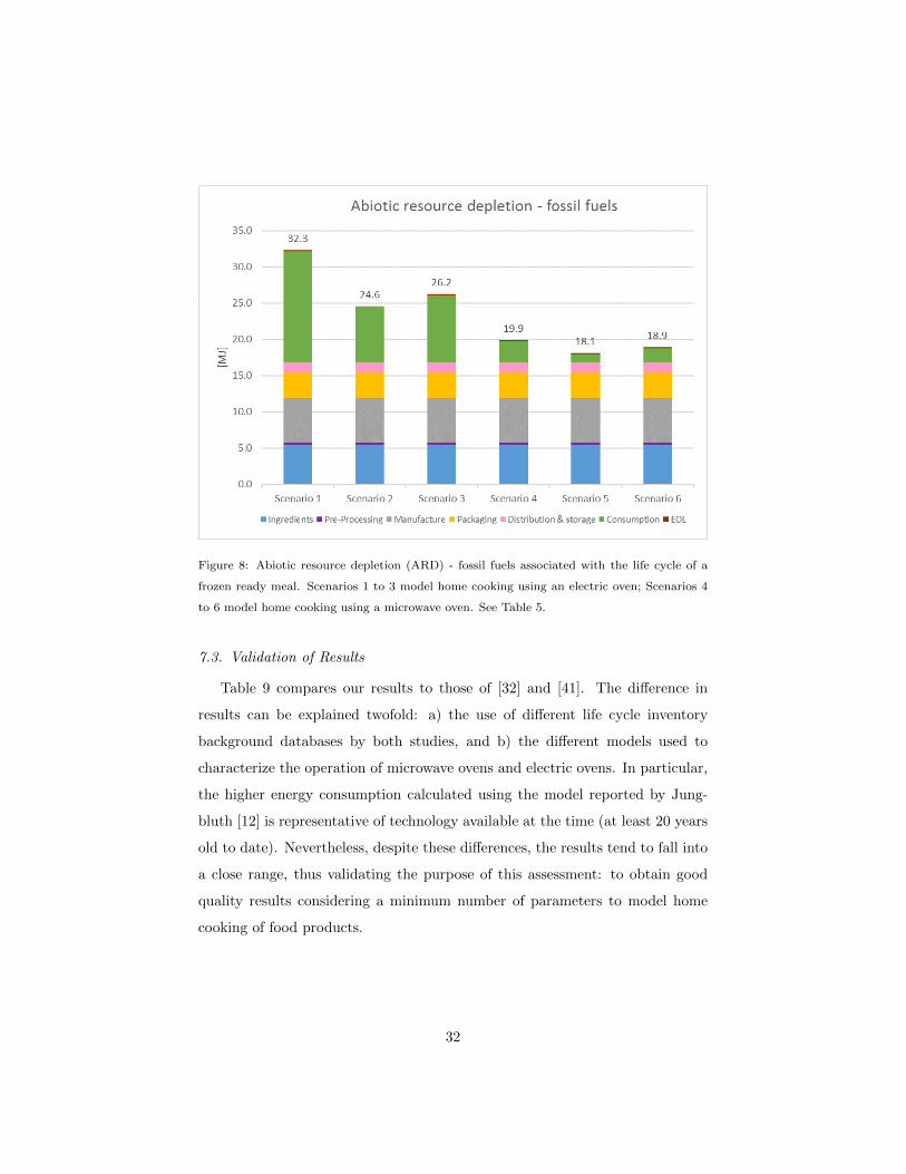
Figure 8: Abiotic resource depletion (ARD) - fossil fuels associated with the life cycle of a

frozen ready meal. Scenarios 1 to 3 model home cooking using an electric oven; Scenarios 4

to 6 model home cooking using a microwave oven. See Table 5.

7.3. Validation of Results

Table 9 compares our results to those of [32] and [41]. The difference in

results can be explained twofold: a) the use of different life cycle inventory

background databases by both studies, and b) the different models used to

characterize the operation of microwave ovens and electric ovens. In particular,

the higher energy consumption calculated using the model reported by Jung-

bluth [12] is representative of technology available at the time (at least 20 years

old to date). Nevertheless, despite these differences, the results tend to fall into

a close range, thus validating the purpose of this assessment: to obtain good

quality results considering a minimum number of parameters to model home

cooking of food products.

32

Scenario Cooking Method

GHG emissions(kg CO2-eq/frozen ready meal)

Abiotic resource depletionfossil fuels

(MJ/frozen ready meal)

OverallConsumption

Stage OverallConsumption

Stage

1

ElectricOven

3.4 1.4 32.3 15.4

2 2.7 0.7 24.6 7.7

3 2.9 0.9 26.2 9.3

RM-8 3.6 1.4 34.0 19.7

4

MicrowaveOven

2.3 0.3 19.9 3.0

5 2.3 0.3 19.9 3.0

6 2.2 0.2 18.9 2.0

RM-7 2.4 0.2 17.7 2.7

Table 9: Environmental impacts associated with a frozen ready meal. Comparison of results

using the proposed model and the model of Schmidt Rivera et al. [32]. RM-8 and RM-7 refer

to two scenarios studied in [32] (see Table 15 in [32]).

8. Conclusion

The conclusions drawn from validating our proposed models in large, geo-

graphically spread datasets, and demonstration in the Food LCA, confirm our

hypothesis that by using only smart meter energy data, without resorting to

other, difficult to obtain, parameters, such as food type, temperature, and

weight, we can build accurate energy consumption models of major cooking

appliances. In Section 4 the models for electric microwaves and ovens were gen-

erated from real consumption data, that implicitly incorporate user behaviour

in usage of the appliances, contrary to relying on manufacturer’s assumptions on

how the appliances should be used and their resulting models. As user behaviour

can impact the amount of energy an appliance consumes, by proposing a model

which uses consumption data from (and is validated on) real homes (unlike pre-

vious studies which have used laboratory tests which do not take into account

inefficient and unusual use cases), we show that, although human behaviour

can cause variations at scale, it is possible to account for this via mathemati-

cal models generated from actual consumer usage data, which can be updated

33

and scaled easily. In Section 5 we demonstrate that the proposed mathematical

models are suitable to estimate appliance energy usage and are generally more

accurate than previous models, reflecting recent trends in market availability

and ownership of more efficient cooking appliances, and possibly more energy-

efficient approaches in cooking practices by households. As these trends will

continue, it is necessary to have a scalable approach to large-scale food LCA as

well as other large longitudinal consumer and energy studies, where information

may be lacking with regards to specialised knowledge such as cooking settings,

food temperature and weight, appliance makes and models. In Section 7, where

the proposed models are compared with other state-of-the-art models used in

the Consumption of Food LCA, we show that our models fall within a close

range of contemporary energy efficient appliance technology consumption com-

pared to non-scalable models proposed 20 years ago. Furthermore, we show that

the Consumption phase of Food LCA is a significant contributor to greenhouse

emissions and abiotic resource depletion. Therefore, the need arises to develop

and update appliance consumption models on a regular basis and at relative

low cost to reflect new technology. In turn, these models provide data that

can satisfy LCA data quality requirements on time-related coverage, technology

coverage, precision and representativeness.

The applicability of the proposed methodology for developing scalable ap-

pliance models from pervasive smart meter data embedding user behaviour is

wide and goes beyond Food LCA. Indeed, from an energy-efficiency perspec-

tive, targeted energy feedback can be provided on consumers appliance usage

habits and activities [29] leading to informed energy savings programmes and

retrofit strategies for replacing appliances. Appliance manufacturers can get a

better understanding of the actual consumption of appliances by customers and

hence improve appliance design and life expectancy and consumption phase of

appliance LCA. In relation to this, our study can augment consumer studies

to identify habits and practices towards appliance repair and second-hand pur-

chases, such as [45], and help meet targets within the waste policy framework.

Furthermore, these models support environmental evaluation of appliances, thus

34

enabling recommendations for the development of eco-design regulations in the

EU, e.g., see [46].

Acknowledgements

This project was partly supported by Nestec S.A and carried out at the

University of Strathclyde.

Bibliography

[1] B. Note, BNCK06 : Kettle trends (2006).

[2] G. Edwards-Jones, K. Plassmann, E. H. York, B. Hounsome, D. L. Jones,

L. Mila i Canals, Vulnerability of exporting nations to the development of

a carbon label in the United Kingdom, Environmental Science and Policy

12 (4) (2009) 479–490. doi:10.1016/j.envsci.2008.10.005.

[3] C. Thim, Domestic Appliances, in: H.-J. Bullinger (Ed.), Technology

Guide, Principles ??? Applications ??? Trends, Springer US, 2009, pp.

458–461. doi:10.1007/978-3-540-88546-7.

[4] U. Sonesson, H. Janestad, B. Raaholt, Energy for Preparation and Storing

of Food - Models for calculation of energy use for cooking and cold storage

in households, no. 709, 2003.

[5] T. J. Hager, R. Morawicki, Energy consumption during cooking in the

residential sector of developed nations: A review, Food Policy 40 (2013)

54–63. doi:10.1016/j.foodpol.2013.02.003.

URL http://dx.doi.org/10.1016/j.foodpol.2013.02.003

[6] C. E. Dutilh, K. J. Kramer, Energy Consumption in the Food Chain, AM-

BIO: A Journal of the Human Environmentdoi:10.1579/0044-7447-29.

2.98.

35

[7] A. D. Cuellar, M. E. Webber, An updated estimate for energy use in U.S.

food production and policy implications, in: Proceedings of the ASME 4th

International Conference on Energy Sustainability, Vol. 1, 2010, pp. 35–44.

doi:10.1115/ES2010-90179.

[8] M. C. Heller, G. Keoleian, Life cycle-based sustainability indicators for

assessment of the U.S. food system, Report - Center for Sustainable Sys-

tems, School of Natural Resources and Environment, University of Michi-

gan (CSS00-04) (2000) 59 pp.

[9] P. Bertoldi, B. Atanasiu, Electricity consumption and efficiency trends in

the enlarged European Union - Status Report 2009, 2009.

[10] International Energy Agency, World Energy Outlook 2006, World Energy

Outlookdoi:10.1787/weo-2006-en.

URL http://books.google.com/books?hl=en&lr=&id=

JAcuHqDnI6gC&oi=fnd&pg=PA3&dq=World+Energy+Outlook+

2006&ots=NCadW-C961&sig=5wr-ct_hWTzqi4Rlwo8Gl8L6Ax0

[11] D. K. De, N. M. Shawhatsu, N. N. De, M. I. Ajaeroh, Energy-efficient

cooking methods, Energy Efficiency 6 (1) (2013) 163–175. doi:10.1007/

s12053-012-9173-7.

[12] N. Jungbluth, Life-Cycle-Assessment for Stoves and Ovens (1997) 1–52.

[13] S. Lakshmi, A. Chakkaravarthi, R. Subramanian, V. Singh, Energy con-

sumption in microwave cooking of rice and its comparison with other do-

mestic appliances, Journal of Food Engineering 78 (2) (2007) 715–722.

doi:10.1016/j.jfoodeng.2005.11.011.

[14] T. Das, R. Subramanian, A. Chakkaravarthi, V. Singh, S. Z. Ali, P. K.

Bordoloi, Energy conservation in domestic rice cooking, Journal of Food

Engineering 75 (2) (2006) 156–166. doi:10.1016/j.jfoodeng.2005.04.

005.

36

[15] J. Zufia, L. Arana, Life cycle assessment to eco-design food products: in-

dustrial cooked dish case study, Journal of Cleaner Production 16 (17)

(2008) 1915–1921. doi:10.1016/j.jclepro.2008.01.010.

[16] L. A. Calderon, L. Iglesias, A. Laca, M. Herrero, M. Dıaz, The utility of Life

Cycle Assessment in the ready meal food industry, Resources, Conserva-

tion and Recycling 54 (12) (2010) 1196–1207. doi:10.1016/j.resconrec.

2010.03.015.

[17] L. A. Calderon, M. Herrero, A. Laca, M. Dıaz, Environmental impact

of a traditional cooked dish at four different manufacturing scales: from

ready meal industry and catering company to traditional restaurant and

homemade, International Journal of Life Cycle Assessment (2017) 1–

13doi:10.1007/s11367-017-1326-7.

[18] C. Oberascher, R. Stamminger, C. Pakula, Energy efficiency in daily food

preparation, International Journal of Consumer Studies 35 (2) (2011) 201–

211. doi:10.1111/j.1470-6431.2010.00963.x.

[19] Vattenfall, Energiesparen macht Spaß und spart Geld, Tech. rep. (2008).

[20] G. Wood, M. Newborough, Dynamic energy-consumption indicators for do-

mestic appliances: Environment, behaviour and design, Energy and Build-

ings 35 (8) (2003) 821–841. doi:10.1016/S0378-7788(02)00241-4.

[21] E. A. DeMerchant, User’s Influence on Energy Consumption with Cooking

Systems Using Electricity, Virginia Polytechnic Institute and State Univer-

sity (1997) 1–155.

URL http://hdl.handle.net/10919/29838

[22] R. Kemna, Energy Consumption of Domestic Appliances in European

Households, Tech. rep. (2010).

[23] F. Burlon, Energy Efficiency of Combined Ovens, in: Energy Procedia,

Vol. 82, Elsevier B.V., 2015, pp. 986–993. doi:10.1016/j.egypro.2015.

11.856.

37

[24] D. Papasidero, S. Pierucci, F. Manenti, Energy optimization of bread

baking process undergoing quality constraints, Energy 116 (2016) 1–6.

doi:10.1016/j.energy.2016.06.046.

URL http://dx.doi.org/10.1016/j.energy.2016.06.046

[25] A. Milani, C. Camarda, L. Savoldi, A simplified model for the electrical

energy consumption of washing machines, Journal of Building Engineering

2 (2015) 69–76. doi:10.1016/j.jobe.2015.04.007.

URL http://dx.doi.org/10.1016/j.jobe.2015.04.007

[26] J. Geppert, Modelling of domestic refrigerators’ energy consumption under

real life conditions in Europe (2011) 145.

[27] P. Jason, I. Cooper, Smart metering implementation programme govern-

ment response to the consultation on the second version of the smart me-

tering equipment technical specifications part 1 (January) (2013) 14.

[28] D. Murray, J. Liao, L. Stankovic, V. Stankovic, Understanding usage

patterns of electric kettle and energy saving potential, Applied Energy 171

(2016) 231–242. doi:10.1016/j.apenergy.2016.03.038.

URL http://www.sciencedirect.com/science/article/pii/

S0306261916303579

[29] L. Stankovic, V. Stankovic, J. Liao, C. Wilson, Measuring the energy in-

tensity of domestic activities from smart meter data, Applied Energy 183

(2016) 1565–1580. doi:10.1016/j.apenergy.2016.09.087.

URL http://dx.doi.org/10.1016/j.apenergy.2016.09.087

[30] M. Pipattanasomporn, M. Kuzlu, S. Rahman, Y. Teklu, Load Profiles of

Selected Major Household Appliances and Their Demand Response Oppor-

tunities 5 (2) (2014) 742–750.

[31] J. Riley, J. Hulme, Report 9: Domestic appliances, cooking & cooling

equipment, Tech. rep., BRE, Department of Energy and Climate Change

(DECC) (2013).

38

[32] X. C. Schmidt Rivera, N. Espinoza Orias, A. Azapagic, Life cycle envi-

ronmental impacts of convenience food: Comparison of ready and home-

made meals, Journal of Cleaner Production 73 (2014) (2014) 294–309.

doi:10.1016/j.jclepro.2014.01.008.

URL http://dx.doi.org/10.1016/j.jclepro.2014.01.008

[33] B. Zhao, L. Stankovic, V. Stankovic, On a Training-Less Solution for Non-

Intrusive Appliance Load Monitoring Using Graph Signal Processing, IEEE

Access 4 (2016) 1784–1799. doi:10.1109/ACCESS.2016.2557460.

[34] J. Kelly, W. Knottenbelt, The UK-DALE dataset, domestic appliance-level

electricity demand and whole-house demand from five UK homes., Scientific

data 2 (2015) 150007. arXiv:1404.0284, doi:10.1038/sdata.2015.7.

URL http://arxiv.org/abs/1404.0284

[35] D. Murray, L. Stankovic, V. Stankovic, An electrical load measurements

dataset of United Kingdom households from a two-year longitudinal study

4463 (2016) 1–12. doi:10.1038/sdata.2016.122.

[36] C. Beckel, W. Kleiminger, R. Cicchetti, T. Staake, S. Santini, The ECO

Data Set and the Performance of Non-Intrusive Load Monitoring Algo-

rithms, Proceedings of the 1st ACM Conference on Embedded Systems for

Energy-Efficient Buildings (2014) 80—-89doi:10.1145/2674061.2674064.

[37] N. Batra, M. Gulati, A. Singh, M. B. Srivastava, It’s Different: In-

sights into home energy consumption in India, Proceedings of the 5th

ACM Workshop on Embedded Systems For Energy-Efficient Buildings -

BuildSys’13 (November) (2013) 1–8. doi:10.1145/2528282.2528293.

URL http://dl.acm.org/citation.cfm?doid=2528282.2528293

[38] K. He, L. Stankovic, J. Liao, V. Stankovic, Non-Intrusive Load Disaggre-

gation using Graph Signal Processing, IEEE Transactions on Smart Grid

3053 (c) (2016) 1–1. doi:10.1109/TSG.2016.2598872.

URL http://ieeexplore.ieee.org/document/7539273/

39

[39] H. Altrabalsi, V. Stankovic, J. Liao, L. Stankovic, Low-complexity energy

disaggregation using appliance load modelling, AIMS Energy 4 (1) (2016)

1–21. doi:10.3934/energy.2016.1.1.

[40] J. Z. Kolter, M. J. Johnson, REDD : A Public Data Set for Energy

Disaggregation Research, SustKDD workshop xxxxx (1) (2011) 1–6.

URL http://users.cis.fiu.edu/~lzhen001/activities/

KDD2011Program/workshops/WKS10/doc/SustKDD3.pdf

[41] X. Bengosa, T. Nemecek, V. Rossi, J. Lansche, S. Humbert, P. Mouron,

World Food LCA Database (August).

[42] Intergovernmental Panel on Climate Change, Climate change 2013: The

physical science basis, CLIMATE CHANGE 2013 - They Physical Science

Basis.

[43] L. van Oers, CML-IA Characterisation Factors, Tech. rep.

URL http://cml.leiden.edu/software/data-cmlia.html

[44] P. Sustainability, SimaPro Life Cycle Assessment software (2016).

[45] V. Perez-Belis, M. Braulio-Gonzalo, P. Juan, M. D. Bovea, Consumer at-

titude towards the repair and the second-hand purchase of small house-

hold electrical and electronic equipment. A Spanish case study, Journal of

Cleaner Production 158 (2017) 261–275. doi:10.1016/j.jclepro.2017.

04.143.

[46] A. Gallego-Schmid, H. K. Jeswani, J. M. F. Mendoza, A. Azapagic, Life

cycle environmental evaluation of kettles: Recommendations for the de-

velopment of eco-design regulations in the European Union, Science of the

Total Environment 625 (2018) 135–146. doi:10.1016/j.scitotenv.2017.

12.262.

URL https://doi.org/10.1016/j.scitotenv.2017.12.262

40