appendix m: wetland value assessment … iii atchafalaya...marsh (more open water conditions) was...
TRANSCRIPT

APPENDIX M:
Wetland Value Assessment (WVA) Model Report

Volume III – Convey Atchafalaya River Water to Northern Terrebonne Marshes and Multipurpose
Operation of Houma Navigation Lock – Appendix M – Wetland Value Assessment (WVA)
M-2
Volume III
APPENDIX M:
Wetland Value Assessment (WVA) Model Report
Table of Contents
1.0 Wetland Value Assessment Model .......................................................................... 3 2.0 Wetland Acreage Projections ................................................................................... 5
2.1 PREDICTING NET WETLAND BENEFITS OF MARSH CREATION MEASURES (E.G. TERRACING AND MARSH BERM MEASURES) ...................................................................... 6 2.2 PREDICTING NET WETLAND BENEFITS OF MARSH NOURISHMENT MEASURES (E.G. MEASURE CD7) ................................................................................................................ 8 2.3 PREDICTING NET WETLAND BENEFITS OF SHORELINE PROTECTION MEASURES (E.G. MEASURE WO2) ............................................................................................................. 10 2.4 PREDICTING WETLAND BENEFITS OF FRESHWATER INTRODUCTIONS ...................... 12
3.0 Wetland Acreage Predictions under Increased SLR Scenarios ............................. 16 4.0 Literature Cited ...................................................................................................... 17
Annexes Annex 1 FWS Comments on WVA Certification Annex 2 SAND2 Model Verification Annex 3 Quantifying Benefits of Freshwater Flow Diversion to Coastal Marshes:
Theory and Applications Annex 4 SAND2 and WVA Data Summary Tables

Volume III – Convey Atchafalaya River Water to Northern Terrebonne Marshes and Multipurpose
Operation of Houma Navigation Lock – Appendix M – Wetland Value Assessment (WVA)
M-3
Methodology for Determining Environmental Benefits 1.0 Wetland Value Assessment Model
The HET/PDT agreed that use of the Wetland Value Assessment (WVA) methodology would be most appropriate given the tight feasibility study schedule. The Wetland Value Assessment (WVA) model was developed under the Coastal Wetlands Planning, Protection, and Restoration program for determining benefits of proposed coastal wetland restoration projects. The 2009 version was used to assess benefits for diversions and other features proposed under this project. Further information on this model may be obtained from the U.S. Fish and Wildlife Service’s Lafayette Louisiana Ecological Services Field Office (Phone: 337-291-3101). The WVA is similar to the U.S. Fish and Wildlife Service’s Habitat Evaluation Procedures (HEP) in that habitat quality and quantity are measured for baseline conditions and predicted for future without-project and future with-project conditions. Separate models were used for cypress-tupelo swamp, fresh/intermediate marsh, brackish marsh, and saline marsh. Instead of the species-based approach of HEP, each WVA model utilizes an assemblage of variables considered important to the suitability of that habitat type for supporting a diversity of fish and wildlife species. As with HEP, the WVA allows for a numeric comparison of each future condition and provides a quantitative estimate of project-related impacts to fish and wildlife resources. The WVA models operate under the assumption that optimal conditions for fish and wildlife habitat within a given coastal wetland type can be characterized, and that existing or predicted conditions can be compared to that optimum to provide an index of habitat quality. Habitat quality is estimated and expressed through the use of a mathematical model developed specifically for each wetland type. Each model consists of: 1) a list of variables that are considered important in characterizing fish and wildlife habitat; 2) a Suitability Index graph for each variable, which defines the assumed relationship between habitat quality (Suitability Index) and different variable values; and 3) a mathematical formula that combines the Suitability Indices for each variable into a single value for wetland habitat quality, termed the Habitat Suitability Index (HSI). The WVA models assess the suitability of each habitat type for providing resting, foraging, breeding, and nursery habitat to a diverse assemblage of fish and wildlife species. This standardized, multi-species, habitat-based methodology facilitates the assessment of project-induced impacts on fish and wildlife resources. HSI values are determined for each target year. Target years, determined by the model user, represent when significant changes in habitat quality or quantity were expected during the 50-year period of analysis, under future with-project and future without-project conditions. In this study, target years of 0, 1, 10, and 50 are evaluated. The product of an HSI value and the acreage of available habitat for a given target year is known as the Habitat Unit (HU). The HU is the basic unit for measuring project effects on fish and wildlife habitat. Future HUs change according to changes in habitat quality
Volume III – Convey Atchafalaya River Water to Northern Terrebonne Marshes and Multipurpose
Operation of Houma Navigation Lock – Appendix M – Wetland Value Assessment (WVA)
M-4
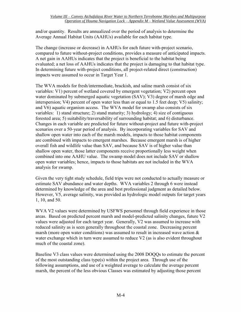
and/or quantity. Results are annualized over the period of analysis to determine the Average Annual Habitat Units (AAHUs) available for each habitat type. The change (increase or decrease) in AAHUs for each future with-project scenario, compared to future without-project conditions, provides a measure of anticipated impacts. A net gain in AAHUs indicates that the project is beneficial to the habitat being evaluated; a net loss of AAHUs indicates that the project is damaging to that habitat type. In determining future with-project conditions, all project-related direct (construction) impacts were assumed to occur in Target Year 1. The WVA models for fresh/intermediate, brackish, and saline marsh consist of six variables: V1) percent of wetland covered by emergent vegetation; V2) percent open water dominated by submerged aquatic vegetation (SAV); V3) degree of marsh edge and interspersion; V4) percent of open water less than or equal to 1.5 feet deep; V5) salinity; and V6) aquatic organism access. The WVA model for swamp also consists of six variables: 1) stand structure; 2) stand maturity; 3) hydrology; 4) size of contiguous forested area; 5) suitability/traversability of surrounding habitat; and 6) disturbance. Changes in each variable are predicted for future without-project and future with-project scenarios over a 50-year period of analysis. By incorporating variables for SAV and shallow open water into each of the marsh models, impacts to those habitat components are combined with impacts to emergent marshes. Because emergent marsh is of higher overall fish and wildlife value than SAV, and because SAV is of higher value than shallow open water, those latter components receive proportionally less weight when combined into one AAHU value. The swamp model does not include SAV or shallow open water variables; hence, impacts to those habitats are not included in the WVA analysis for swamp. Given the very tight study schedule, field trips were not conducted to actually measure or estimate SAV abundance and water depths. WVA variables 2 through 6 were instead determined by knowledge of the area and best professional judgment as detailed below. However, V5, average salinity, was provided as hydrologic model outputs for target years 1, 10, and 50. WVA V2 values were determined by USFWS personnel through field experience in those areas. Based on predicted percent marsh and model-predicted salinity changes, future V2 values were adjusted for each target year. Generally, V2 was assumed to increase with reduced salinity as is seen generally throughout the coastal zone. Decreasing percent marsh (more open water conditions) was assumed to result in increased wave action & water exchange which in turn were assumed to reduce V2 (as is also evident throughout much of the coastal zone). Baseline V3 class values were determined using the 2008 DOQQs to estimate the percent of the most outstanding class type(s) within the project area. Through use of the following assumptions, and use of a weighted average to calculate the average percent marsh, the percent of the less obvious Classes was estimated by adjusting those percent
Volume III – Convey Atchafalaya River Water to Northern Terrebonne Marshes and Multipurpose
Operation of Houma Navigation Lock – Appendix M – Wetland Value Assessment (WVA)
M-5
Class types until the resulting average percent marsh equaled that predicted for that given target year using the marsh loss prediction methods:
V3 Class 1 assumed to represent 90% marsh V3 Class 2 assumed to represent 75% marsh V3 Class 3 assumed to represent 50% marsh V3 Class 4 assumed to represent 25% marsh V3 Class 5 assumed to represent 10% marsh Average percent marsh = (0.95* %class1) + (0.75* %class2) + (0.50 * %class3) +(0.25 * %class4) + (0.10 * %class5)
Future V3 values were estimated by adjusting baseline percent class values to reflect anticipated wetland loss processes (e.g. loss due primarily to shoreline erosion, loss due to break-up of interior marshes). Those values were adjusted so that the weighted average percent marsh equaled that predicted for that given target year using the marsh loss prediction methods.
Baseline V4 values were estimated by USFWS personnel based on field experience. Given that interior break-up usually results in conversion of marsh to shallow water initially and then later to deeper water, FWOP and FWP V4 values were assumed to change roughly in proportion to decreases in V1. Baseline V5 values were provided by hydraulic model results, as were future FWOP and FWP V5 values. Hydraulic modeling was used to predict FWOP and FWP average monthly salinities from one or more representative locations within each wetland receiving area. Using those monthly salinities, average annual salinities were then calculated for each wetland receiving area and used as input into the WVA. V6 values remained fixed at 1.0 for all measures. Where canal plugs were evaluated, typically V6 would be adjusted to reflect reduced fisheries access. That was not done for the ARTM evaluations for the following reasons:
a) The proposed plugs were on man-made canals deemed to have caused significant adverse hydrologic modifications harmful to area wetlands and because those canals resulted in artificially increased fisheries access.
b) Other natural and man-made waterways are available to provide fisheries access. Use of typical V6 values for canal plugs would result in little or no project benefits, implying that perceived impacts to fisheries access would supersede and preclude virtually all hydrologic restoration efforts and specifically measures designed to correct major canal-induced hydrologic alternations. 2.0 Wetland Acreage Projections
The estimates of FWP and FWOP marsh acreages required for variable V1 in the WVA are the most important variable and the most difficult variable to determine. Described
Volume III – Convey Atchafalaya River Water to Northern Terrebonne Marshes and Multipurpose
Operation of Houma Navigation Lock – Appendix M – Wetland Value Assessment (WVA)
M-6
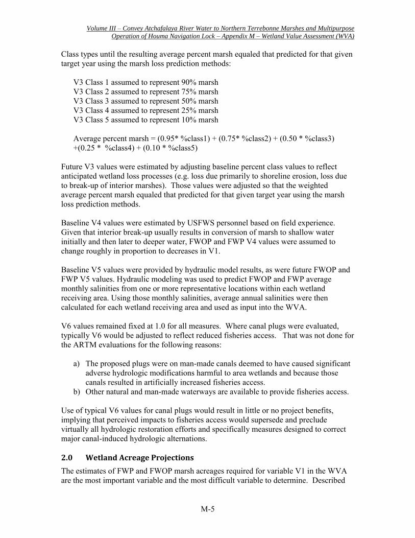
below are the models and methods used to determine those marsh acreages for various types of measures analyzed in this study and the methods for predicted benefits of the proposed project alternatives. Wetland acreage data (1985 through 2008) was obtained from the USGS for each of the study area subunits. Future-without-project (FWOP) subunit wetland acreages were determined via a linear trendline through those data (Figure 1). Where applicable, annual net acreage benefits associated with pre-existing or soon to be constructed restoration projects were added to the subunit FWOP acreages to obtain revised FWOP subunit acreages. Figure 1. Actual and predicted acreage for the G2,G3,G6 subunit.
2.1 Predicting Net Wetland Benefits of Marsh Creation Measures (e.g. terracing and
marsh berm measures)
A mathematical model or formula was developed to calculate net marsh creation project benefits (net acres = future-with project acres minus future without project acres; see Annex 4 for calculated acres of benefit from marsh creation measures). Formula inputs include: 1. Created acres – The number of acres of open water filled to create marsh 2. Year constructed – The year in which the marsh creation project is built 3. Loss rate (ac/yr) – The number of created marsh acres being lost each year 4. Subsidence – Corps subsidence rate (ft/century)
10,000
12,000
14,000
16,000
18,000
20,000
22,000
24,000
26,000
28,000
30,000
1980
1990
2000
2010
2020
2030
2040
2050
2060
2070
Wetl
an
d A
cre
s

Volume III – Convey Atchafalaya River Water to Northern Terrebonne Marshes and Multipurpose
Operation of Houma Navigation Lock – Appendix M – Wetland Value Assessment (WVA)
M-7
5. FWP year benefits loss rate reverts – The year in which the reduced post-construction loss rate reverts to the pre-construction or baseline rate.
Model Assumptions: The created marsh loss rate is initially 50% of the loss rate of existing surrounding areas provided post-construction submergence (SLR + subsidence) is less than 10 inches (McGinnis 1997). The 50% loss rate reduction is a consensus assumption of agency and academic personnel based on known processes. The general consensus is that this assumption provides a conservative benefit estimate, provided the project is correctly engineered and constructed. With relative sea level rise, accretion must occur for marshes to survive. Over time, as the created marsh surface subsides and new accretion occurs, the plants lose contact with the mechanically deposited material. It is assumed that when the rooting depth of 10 inches is no longer in contact with the deposited soil, the marsh soil matrix is like that of the surrounding natural marsh, and, hence, it would be lost at the rate of the natural marshes. For marshes created in year 2016, this rate change would occur in year 2040 under the low sea level rise scenario, in year 2037 under the medium sea level rise scenario, and in year 2031 under the high sea level rise scenario.
Excel Model Formula: =IF(year>=FWP year benefits loss rate reverts,previous acres+FWP loss rate*2,IF(year<build year,0,IF(year>=build year,IF(created acres+(loss rate*(year-build year))<0,0,created acres+(loss rate*(year-build year))))))
Model Function (See Figure 2): a) If present year is greater than the year when loss rate reverts to background rate,
the loss rate will be doubled b) If the present year is less than the construction year, then acreage is equal to zero. c) If present year is equal to year constructed, then the created acres are equal to the
net benefits. d) If the present year is greater than year constructed, then net benefits equals
previous years’ acres minus the loss rate.
Volume III – Convey Atchafalaya River Water to Northern Terrebonne Marshes and Multipurpose
Operation of Houma Navigation Lock – Appendix M – Wetland Value Assessment (WVA)
M-8
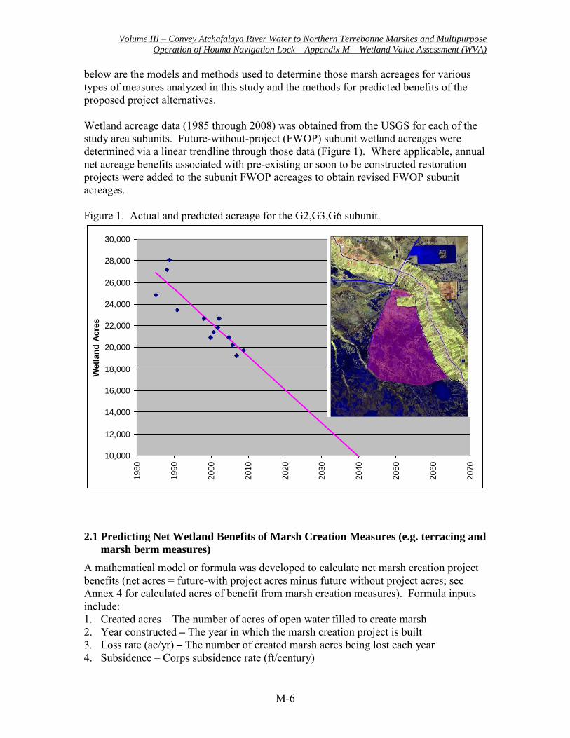
Figure 2. Marsh Creation net benefits, FWOP acres, and FWP acres in relation to time. Acres are added to existing marsh acres in the FWP. The loss rate for the FWOP acres and the created acres will be added together for the FWP acres. After the FWOP acres reach zero, remaining acres will be lost at the loss rate for the created acres.
2.2 Predicting Net Wetland Benefits of Marsh Nourishment Measures (e.g. measure
CD7)
A mathematical model or formula was developed to calculate net marsh nourishment project benefits (net acres = future-with project acres minus future without project acres; see Annex 4 for calculated acres of benefit from marsh nourishment measures). Formula inputs include: 1. Total Acres Nourished – Total area of the project 2. Construction year – The year in which the marsh nourishment project is built. 3. Net annual benefit (ac/yr) – The land loss rate for the nourished area (50% of the
FWOP rate) 4. FWOP zero – The year when the FWOP marsh acreage has reached zero. 5. Subsidence – Corps subsidence rate (ft/century) 6. FWP year benefits loss rate reverts – The year in which the FWP reduced loss rate
reverts to the pre-project rates.
Marsh Creation
-1000
0
1000
2000
3000
4000
5000
6000
2000 2020 2040 2060 2080 2100 2120 2140 2160 2180 2200
Year
Ac
res
-200
0
200
400
600
800
1000
Ne
t B
en
efi
t A
cre
s FWOP
FWP
FWOP w/med SLR
FWP w/med SLR
benefits
benefits w/ med SLR
Volume III – Convey Atchafalaya River Water to Northern Terrebonne Marshes and Multipurpose
Operation of Houma Navigation Lock – Appendix M – Wetland Value Assessment (WVA)
M-9
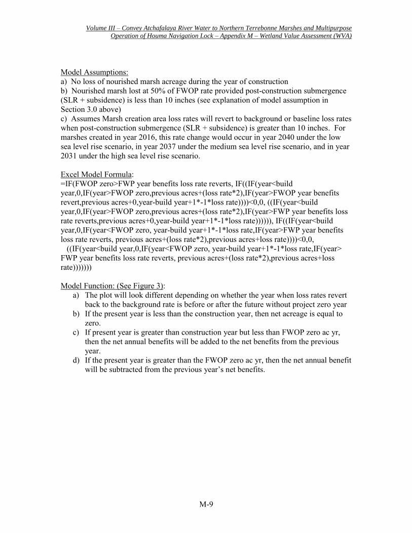
Model Assumptions: a) No loss of nourished marsh acreage during the year of construction b) Nourished marsh lost at 50% of FWOP rate provided post-construction submergence (SLR + subsidence) is less than 10 inches (see explanation of model assumption in Section 3.0 above) c) Assumes Marsh creation area loss rates will revert to background or baseline loss rates when post-construction submergence (SLR + subsidence) is greater than 10 inches. For marshes created in year 2016, this rate change would occur in year 2040 under the low sea level rise scenario, in year 2037 under the medium sea level rise scenario, and in year 2031 under the high sea level rise scenario.
Excel Model Formula: =IF(FWOP zero>FWP year benefits loss rate reverts, IF((IF(year<build year,0,IF(year>FWOP zero,previous acres+(loss rate*2),IF(year>FWOP year benefits revert,previous acres+0,year-build year+1*-1*loss rate))))<0,0, ((IF(year<build year,0,IF(year>FWOP zero,previous acres+(loss rate*2),IF(year>FWP year benefits loss rate reverts,previous acres+0,year-build year+1*-1*loss rate)))))), IF((IF(year<build year,0,IF(year<FWOP zero, year-build year+1*-1*loss rate,IF(year>FWP year benefits loss rate reverts, previous acres+(loss rate*2),previous acres+loss rate))))<0,0, ((IF(year<build year,0,IF(year<FWOP zero, year-build year+1*-1*loss rate,IF(year> FWP year benefits loss rate reverts, previous acres+(loss rate*2),previous acres+loss rate)))))))
Model Function: (See Figure 3): a) The plot will look different depending on whether the year when loss rates revert
back to the background rate is before or after the future without project zero year b) If the present year is less than the construction year, then net acreage is equal to
zero. c) If present year is greater than construction year but less than FWOP zero ac yr,
then the net annual benefits will be added to the net benefits from the previous year.
d) If the present year is greater than the FWOP zero ac yr, then the net annual benefit will be subtracted from the previous year’s net benefits.
Volume III – Convey Atchafalaya River Water to Northern Terrebonne Marshes and Multipurpose
Operation of Houma Navigation Lock – Appendix M – Wetland Value Assessment (WVA)
M-10
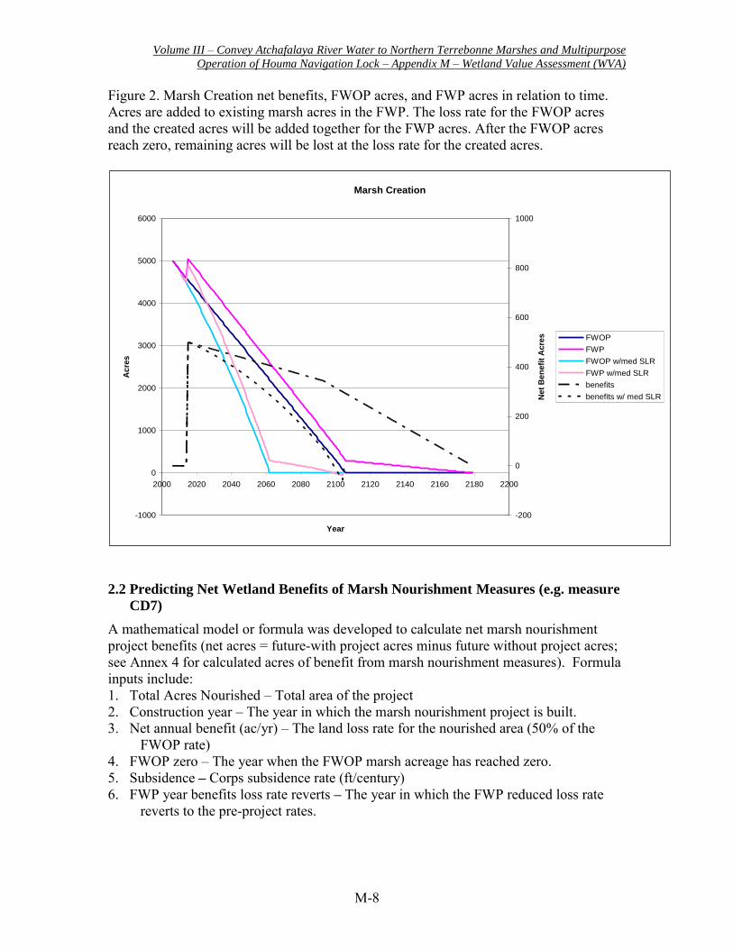
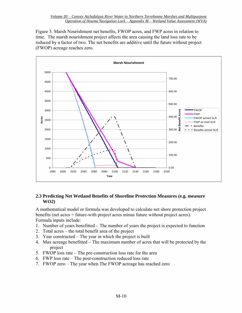
Figure 3. Marsh Nourishment net benefits, FWOP acres, and FWP acres in relation to time. The marsh nourishment project affects the area causing the land loss rate to be reduced by a factor of two. The net benefits are additive until the future without project (FWOP) acreage reaches zero.
2.3 Predicting Net Wetland Benefits of Shoreline Protection Measures (e.g. measure
WO2)
A mathematical model or formula was developed to calculate net shore protection project benefits (net acres = future-with project acres minus future without project acres). Formula inputs include: 1. Number of years benefitted – The number of years the project is expected to function 2. Total acres – the total benefit area of the project 3. Year constructed – The year in which the project is built 4. Max acreage benefitted – The maximum number of acres that will be protected by the
project 5. FWOP loss rate – The pre-construction loss rate for the area 6. FWP loss rate – The post-construction reduced loss rate 7. FWOP zero – The year when The FWOP acreage has reached zero
Marsh Nourishment
0
500
1000
1500
2000
2500
3000
3500
4000
4500
5000
1980 2000 2020 2040 2060 2080 2100 2120 2140 2160 2180 2200
Year
Acre
s
0.00
100.00
200.00
300.00
400.00
500.00
600.00
700.00
Net
Ben
efi
t A
cre
s FWOP
FWP
FWOP w/med SLR
FWP w/ med SLR
Benefits
Benefits w/med SLR

Volume III – Convey Atchafalaya River Water to Northern Terrebonne Marshes and Multipurpose
Operation of Houma Navigation Lock – Appendix M – Wetland Value Assessment (WVA)
M-11
Model Assumptions: a) Assumes no loss during the year of construction b) Assumes 100% reduction in loss rate for as long as the project is maintained. Foreshore armor dikes protecting bank-side marshes have been effective in not only halting bank erosion, but in some cases trapping suspended sediment and promoting accretion between the dike and the existing bank (e.g. CWPPRA project ME-09). Assuming that the foreshore dike is properly engineered and maintained, and that all marsh loss was caused by mechanical wave action, the assumption was made that such a feature would halt bank erosion. c) Projects will be maintained for 50 years d) No effects from sea level rise assuming the project is maintained to accommodate changes in sea level
Excel Model Formula: =IF(IF(year<build year,0,IF(year-build year< # years benefit,((-FWOP loss rate+FWP loss rate)*(year-build year)-(FWOP loss rate-FWP loss rate)), (IF(year>FWOP zero,previous acres+FWOP loss rate,Max acreage benefit calculated))))<0,0,IF(year<build year,0,IF(year-build year<# years benefit,((-FWOP project loss rate+FWP loss rate)*(year-build year)-(FWOP loss rate-FWP loss rate)),(IF(year>FWOP zero,previous acres+FWOP loss rate,Max acreage benefit calculated))))) Model Function (See Figure 4):
a) If the present year is less than the construction year, then net benefit acreage is equal to zero.
b) If present year is greater than construction year but less than FWOP zero ac yr, then the FWP land loss rate will be reduced for the number of years benefitted.
c) If the present year is greater than the FWOP zero ac yr, then the FWOP annual loss will be subtracted from the previous year’s net benefits.
Volume III – Convey Atchafalaya River Water to Northern Terrebonne Marshes and Multipurpose
Operation of Houma Navigation Lock – Appendix M – Wetland Value Assessment (WVA)
M-12
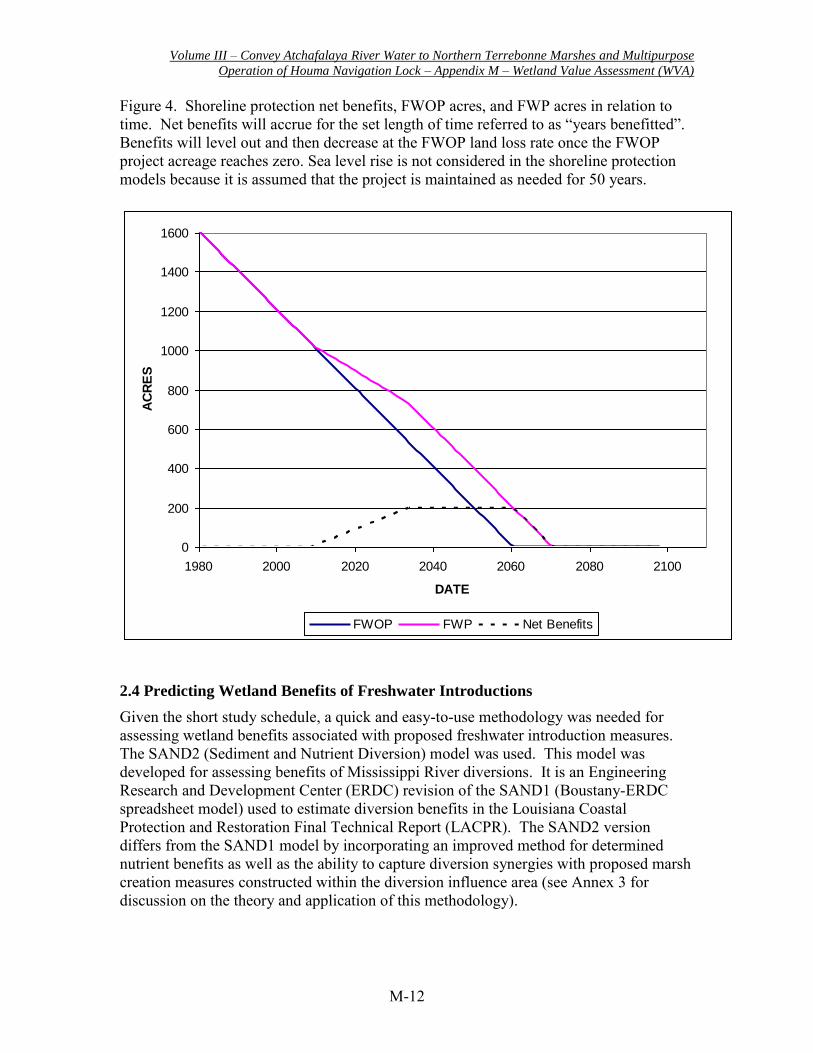
Figure 4. Shoreline protection net benefits, FWOP acres, and FWP acres in relation to time. Net benefits will accrue for the set length of time referred to as “years benefitted”. Benefits will level out and then decrease at the FWOP land loss rate once the FWOP project acreage reaches zero. Sea level rise is not considered in the shoreline protection models because it is assumed that the project is maintained as needed for 50 years.
2.4 Predicting Wetland Benefits of Freshwater Introductions
Given the short study schedule, a quick and easy-to-use methodology was needed for assessing wetland benefits associated with proposed freshwater introduction measures. The SAND2 (Sediment and Nutrient Diversion) model was used. This model was developed for assessing benefits of Mississippi River diversions. It is an Engineering Research and Development Center (ERDC) revision of the SAND1 (Boustany-ERDC spreadsheet model) used to estimate diversion benefits in the Louisiana Coastal Protection and Restoration Final Technical Report (LACPR). The SAND2 version differs from the SAND1 model by incorporating an improved method for determined nutrient benefits as well as the ability to capture diversion synergies with proposed marsh creation measures constructed within the diversion influence area (see Annex 3 for discussion on the theory and application of this methodology).
0
200
400
600
800
1000
1200
1400
1600
1980 2000 2020 2040 2060 2080 2100
DATE
AC
RE
S
FWOP FWP Net Benefits
Volume III – Convey Atchafalaya River Water to Northern Terrebonne Marshes and Multipurpose
Operation of Houma Navigation Lock – Appendix M – Wetland Value Assessment (WVA)
M-13
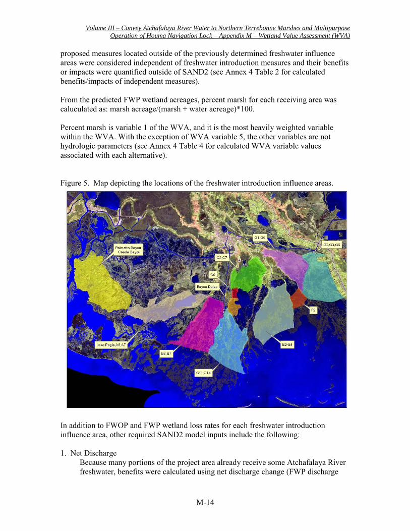
Given the uncertainties regarding future subsidence rate changes, sea-level rise changes, and many other factors that might affect future wetland loss rates over the project life, there is considerable uncertainty regarding the accuracy of the predicted freshwater introduction benefits. Annex 2 below provides results of model verification conducted on the SAND2 model for other freshwater diversion projects, demonstrating its utility in predicting project benefits. It should be noted, however, that these projects involved the diversion of both freshwater and sediment. No examples of freshwater introduction without sediment are available to verify the application of the SAND2 model for nutrient-only situations such as the ARTM study. However, the SAND2 model does provide an objective means for comparing alternative measures and plans as conducted in the ARTM study. Utilizing the predicted FWOP wetland acreage as a basis, the SAND2 model computes FWP acreages by adding benefit acres generated through 2 pathways: sediment and nutrient inputs. The nutrient (nitrogen introduction) benefits (in acres) are calculated as the grams of nitrogen introduced annually (less nitrogen lost through denitrification and export), divided by the grams of nitrogen incorporated in the annual production of the subject wetland type, per acre. Throughout the project area, it was assumed that suspended sediment concentrations were minimal and would not provide land-building benefits. Therefore, the sediment concentration input was set to zero and no benefits were predicted through sediment accretion or land-building. The SAND2 model is used to determine freshwater introduction benefits on a predetermined freshwater introduction influence area. Ideally, hydrologic modeling would be used to determine the extent of the influence area. Given the short study schedule, there was insufficient time for this approach. Instead, a total of 11 separate influence areas were identified based on knowledge of the area, area hydrology, and best professional judgment (Figure 5). The hydraulic model was used to provide predicted FWP and FWOP flows at a number of predetermined points throughout the study area. Those points were established at locations where freshwater inflows entered the predetermined influence areas. Based on model predicted FWOP and FWP flows, net monthly freshwater increase or decrease was calculated for each wetland receiving area. Using observed FWOP wetland acreages for each receiving area, the SAND2 model was run using the calculated net monthly freshwater input changes, together with the monthly nutrient load of those inflows, to compute FWP wetland acreages (see Annex 4 Table 1 for SAND 2 calculated FWP wetland acreages for each receiving area). Indirect effects of outfall management measures were captured in the hydraulic model-generated net discharges used to predict wetland acreage via the SAND2 model, and model-generated salinities (used as variable 5 in the WVA marsh models). Benefits associated with marsh creation measures located within the freshwater input influence areas were incorporated into the benefits generated by the SAND2 model as the nutrient additions associated with freshwater inputs were assumed to reduce both the loss rates of existing natural marshes and the created marshes. Similarly, wetland impacts associated with channel enlargements were in most cases also incorporated into SAND2 model results. If not, those impacts were quantified independently of the SAND2 modeling. All
Volume III – Convey Atchafalaya River Water to Northern Terrebonne Marshes and Multipurpose
Operation of Houma Navigation Lock – Appendix M – Wetland Value Assessment (WVA)
M-14
proposed measures located outside of the previously determined freshwater influence areas were considered independent of freshwater introduction measures and their benefits or impacts were quantified outside of SAND2 (see Annex 4 Table 2 for calculated benefits/impacts of independent measures). From the predicted FWP wetland acreages, percent marsh for each receiving area was caluculated as: marsh acreage/(marsh + water acreage)*100. Percent marsh is variable 1 of the WVA, and it is the most heavily weighted variable within the WVA. With the exception of WVA variable 5, the other variables are not hydrologic parameters (see Annex 4 Table 4 for calculated WVA variable values associated with each alternative). Figure 5. Map depicting the locations of the freshwater introduction influence areas.
In addition to FWOP and FWP wetland loss rates for each freshwater introduction influence area, other required SAND2 model inputs include the following: 1. Net Discharge
Because many portions of the project area already receive some Atchafalaya River freshwater, benefits were calculated using net discharge change (FWP discharge
Volume III – Convey Atchafalaya River Water to Northern Terrebonne Marshes and Multipurpose
Operation of Houma Navigation Lock – Appendix M – Wetland Value Assessment (WVA)
M-15
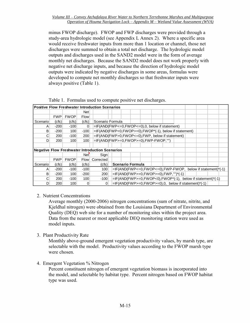
minus FWOP discharge). FWOP and FWP discharges were provided through a study-area hydrologic model (see Appendix L Annex 2). Where a specific area would receive freshwater inputs from more than 1 location or channel, those net discharges were summed to obtain a total net discharge. The hydrologic model outputs and discharges used in the SAND2 model were in the form of average monthly net discharges. Because the SAND2 model does not work properly with negative net discharge inputs, and because the direction of hydrologic model outputs were indicated by negative discharges in some areas, formulas were developed to compute net monthly discharges so that freshwater inputs were always positive (Table 1).
Table 1. Formulas used to compute positive net discharges.
2. Nutrient Concentrations Average monthly (2000-2006) nitrogen concentrations (sum of nitrate, nitrite, and Kjeldhal nitrogen) were obtained from the Louisiana Department of Environmental Quality (DEQ) web site for a number of monitoring sites within the project area. Data from the nearest or most applicable DEQ monitoring station were used as model inputs.
3. Plant Productivity Rate
Monthly above-ground emergent vegetation productivity values, by marsh type, are selectable with the model. Productivity values according to the FWOP marsh type were chosen.
4. Emergent Vegetation % Nitrogen
Percent constituent nitrogen of emergent vegetation biomass is incorporated into the model, and selectable by habitat type. Percent nitrogen based on FWOP habitat type was used.
Net
FWP FWOP Flow
Scenario (cfs) (cfs) (cfs) Scenario Formula
A -200 -100 0 =IF(AND(FWP<=0,FWOP<=0),0, below if statement)
B -200 100 -100 =IF(AND(FWP<0,FWOP>=0),FWOP*(-1), below if statement)
C 200 -100 200 =IF(AND(FWP>0,FWOP<=0),FWP, below if statement)
D 200 100 100 =IF(AND(FWP>=0,FWOP>=0),FWP-FWOP,"")
Net
FWP FWOP Flow Corrected
Scenario (cfs) (cfs) (cfs) Scenario Formula
A -200 -100 -100 =IF(AND(FWP<=0,FWOP<=0),FWP-FWOP, below if statement)*(-1)
B -200 100 -200 =IF(AND(FWP>=0,FWOP>=0),FWP,"")*(-1)
C 200 -100 100 =IF(AND(FWP>=0,FWOP<0),FWOP*(-1), below if statement)*(-1)
D 200 100 0 =IF(AND(FWP>=0,FWOP>=0),0, below if statement)*(-1)
-100
0
Sign
(cfs)
Positive Flow Freshwater Introduction Scenarios
Negative Flow Freshwater Introduction Scenarios
100
200

Volume III – Convey Atchafalaya River Water to Northern Terrebonne Marshes and Multipurpose
Operation of Houma Navigation Lock – Appendix M – Wetland Value Assessment (WVA)
M-16
5. Denitrification Rate A literature reported value of 21g/m2/yr was used (Delaune and Jugsujinda 2003). Denitrification was assumed to reduce the amount of introduced nitrogen available for uptake by emergent wetland vegetation.
6. Marsh Creation Acreage Where marsh creation or terracing projects were proposed within a freshwater introduction influence area, the created acreage was supplied as a SAND2 model input at target year 1 (TY1) so that freshwater introduction benefits would apply to those created acreages and/or terraces.
The SAND2 model requires input of FWOP and FWP wetland loss rates, plus initial marsh and water acreages of the receiving area. FWOP target year 0 (TY0) acreages (year 2015) were determined via application of a linear trendline as described above.
The SAND2 model was developed to allow input of up to 3 different FWOP and 3 different FWP loss rates. Because Coastal Wetland Planning and Protection, and Restoration Act (CWPPRA) projects have a 20-yr project life, implementation of CWPPRA projects within the study area may cause FWOP loss rates to change several times. If several CWPPRA projects occur within a subunit, they may result in more than 3 FWOP loss rate changes over the analysis period. In other freshwater introduction areas, FWP marsh creation or other project measures also resulted in wetland loss rate changes. Whenever there were more than 3 loss rate changes over the modeled evaluation period, a weighted average was utilized to combine similar loss rate periods so that there would be no more than 3 loss rates per evaluation period. FWP loss rates were assumed to equal the FWOP loss rates except where marsh creation, terrace creation, or other FWP measures would be constructed within the freshwater introduction evaluation area. Under those conditions, FWP loss rates would differ from FWOP loss rates. To calculate area FWP loss rates, the net benefits of the individual measures were added to the FWOP acres to obtain FWP area acreage, without freshwater introduction effects. Loss rates are calculated as Acres TY(x-1) – Acres TY(x). The SAND2 model reports FWOP, FWP, and net acres. Because a model flaw was discovered in the computation of some FWOP acreages, the resulting net acreages would not be correct. Therefore instead of using the output net acres, the FWP acres were used and compared to the FWOP acres generated from the linear trendlines as discussed earlier.
3.0 Wetland Acreage Predictions under Increased SLR Scenarios
As described above, linear trendlines (through the 1985 to 2008 wetland acreages obtained from the USGS) were used to determine baseline wetland loss rates for each
Volume III – Convey Atchafalaya River Water to Northern Terrebonne Marshes and Multipurpose
Operation of Houma Navigation Lock – Appendix M – Wetland Value Assessment (WVA)
M-17
project area subunit. Those rates incorporate an assumed static sea level rise (SLR) rate of 2.28 mm/yr. Those baseline loss rates were used as a basis for calculating wetland loss rates under increased SLR scenarios. Water level rise data from the Grand Isle and Eugene Island gages was used to determine that the baseline (year 2004) relative sea level rise (RSLR) equals 11.15 mm/yr. This gage-derived RSLR rate was then reduced by the average study area back-marsh accretion value of 10.2 mm/yr to calculate a baseline accretion-adjusted RSLR rate of 0.95 mm/yr. By adding predicted eustatic sea level rise (SLR) estimates provided by the Corps, future RSLR rates were determined annually for the medium and high SLR scenarios. According to Corps estimates, increased SLR rates begin to occur in 2005. Likewise, wetland loss rates begin accelerating in 2005. To calculate future wetland loss rates under the medium and high SLR scenarios, the baseline wetland loss rate, in acres lost per year, was multiplied by the year X submergence rate ratio (i.e., Accretion-adjusted RSLR Year X/Baseline Accretion-adjusted RSLR Rate from 2004). In this manner, wetland loss rates were calculated for every year of the 50-year project life. Because of accelerating SLR, the wetland loss rates increase every year under the medium and high SLR scenarios. Given that the SAND2 model can incorporate only 3 different loss rates, the 50-year project life was split evenly into 3 periods and an average loss rate was determined for each period. All wetland acreage predictions under the medium and high SLR scenarios used the average loss rates from those 3 periods. In addition to using those increased wetland loss rates, the average water depth input to the SAND2 model was increased to reflect increased water depths. Given that the medium SLR scenario would result in approximately a 6-inch water level increase by TY25, the baseline average water was increased by 0.5 feet. Similarly, the baseline average water depth was increased by 1.0 feet under the High SLR scenario. 4.0 Literature Cited
Delaune, R.D. and A. Jugsujinda. 2003. Denitrification potential in a Louisiana wetland receiving diverted Mississippi River water. Chemistry and Ecology. Vol. 16, Issue 6, pages 411-418.
McGinnis, T.E. II. 1997. Factors of soil strength and shoreline movement in a Louisiana coastal marsh. MS Thesis, University of Southwestern Louisiana, Lafayette, LA.
Snedden, G.A., J.E. Cable, C. Swarzenski, and E. Swenson. 2006. Sediment discharge into a subsiding Louisiana deltaic estuary through a Mississippi River diversion. Estuarine, Coastal and Shelf Science (2006), doi:10.1016/j.ecss.2006.06.035.
Volume III – Convey Atchafalaya River Water to Northern Terrebonne Marshes and Multipurpose
Operation of Houma Navigation Lock – Appendix M – Wetland Value Assessment (WVA)
Annex 1
FWS Comments on WVA Model Certification
FWS Comments on WVA Model Certification Relative to the LCA Convey
Atchafalaya River Water to Northern Terrebonne Marshes (ARTM) Project
February 10, 2010
General FWS Comments: The deadline for completion of LCA project evaluations preceded the resolution of issues raised through the WVA model certification process. Hence, this LCA project had to utilize the un-certified WVA models evaluated in the certification process.
Comment #1: Starting the SI curves for all variables at 0.1 is problematic because even
habitat with no ecological value appears to have some ecological value.
FWS Response: Habitats with no ecological value were excluded from the project area. The project area consists of marsh and associated open water habitat. Even areas consisting of 100% open water have habitat value to many species of fish and wildlife. Hence, an SI of 0.1 is not inappropriate for 100% open water.
Comment #2: Justification for assigning variable weights needs to be provided.
FWS response: Agree. In the development of the WVA models in the early 1990s, variable weighting began with the assumption that certain variables (V1, V2, and V6) were the most important in determining habitat quality and should contribute the greatest amount to the overall Habitat Suitability Index (HIS) value. V1 was deemed as the most important as vegetated marsh is the backbone of the coastal ecosystem. Therefore, those 3 variables were grouped in a term which would allow them to contribute the most to the HSI value. Variables weights were then determined via variable-Suitability Index (SI)- HSI sensitivity tests which involved carefully investigating the effect of each variable onthe HSI. In most instances, it was the best professional judgment of the model developers to determine the final variable weights. Variable weights were not modified for the WVA models utilized for the ARTM Project as model modification was not considered by the Habitat Evaluation Team (HET). The WVA models used are those which were reviewed by the certification panel.
Comment #3: The number of target years should be increased to improve the predictive
ability of the models given that changes are often non-linear.
FWS Response: In some instances, greater precision/accuracy can be achieved by increasing the number of target years. The HET was not of the opinion that increasing the
Volume III – Convey Atchafalaya River Water to Northern Terrebonne Marshes and Multipurpose
Operation of Houma Navigation Lock – Appendix M – Wetland Value Assessment (WVA)
number of target years would improve the accuracy of the benefits assessment. In addition, very short study deadlines required the use of a simplified approach. Comment #4: In the spreadsheet for the marsh models, open water and emergent marsh
AAHUs are incorrectly combined and should be added rather than taking the weighted
arithmetic mean (model issue).
FWS Response: The manner in which marsh and open water AAHUs are combined is standard procedure for the WVA marsh models and was not modified by the HET. The WVA marsh models were developed to provide a higher weighting to marsh benefits as opposed to benefits resulting from the enhancement of open water habitat. This was incorporated to ensure that benefits to wetlands clearly provide the driving force behind project benefits. The HET was not of the opinion that the AAHUs are incorrectly combined.
Comment #6: Sea level is an important phenomenon and relative sea level rise and
climate change should be included in the models. FWS Response: Variable 1 (% marsh) is determined by extrapolating wetland loss rates derived from the past 10 to 20 years using land-water data for the study area. It is assumed that those loss rates are heavily influenced by relative sea level rise. FWS developed a methodology for modifying those baseline wetland loss rates to reflect impacts of future increased sea level rise. That methodology was incorporated in the projections of future without-project and future with-project for the Recommended Plan (RP).
Comment # 10: For some model variables, policy decisions appear to supersede what is
known about the ecology and hydrology of the relationships.
FWS Response: That is correct. CWPPRA program policy did require that some variable habitat relationships, particularly Variable 1 (% emergent marsh), be altered to coincide with program objectives. An adjustment was made in the original WVA development to provide greater benefits to projects which increase emergent marsh, even to a 100% marsh condition. Although not entirely ecologically correct, given Louisiana’s coastal wetland loss crisis, an area of 100% marsh will in the future likely degrade to a more optimal land/water ratio. Hence, a philosophy has arisen that more benefits will accrue over time if an area can be restored to 100% marsh, than to a lesser percentage.
Comment #11: The spreadsheets for the models as created are likely to lead to errors in
maintenance and use.
Volume III – Convey Atchafalaya River Water to Northern Terrebonne Marshes and Multipurpose
Operation of Houma Navigation Lock – Appendix M – Wetland Value Assessment (WVA)
FWS Response: Study deadlines did not allow time for a redesign of current WVA spreadsheets. The HET did review the WVA spreadsheets to reduce the likelihood of errors.
Comment #12: Several inaccuracies were identified in the model spreadsheets that
should be corrected (spreadsheet issue).
FWS Response: Spreadsheet errors indicated in the certification panel’s comments do not impact the models used for the ARTM WVAs. Comment # 15: The WVA method should be expanded to handle risk and uncertainty in
areas exposed to episodic events.
FWS Response: Effects of past episodic events are included in the time period selected to obtain the wetland acreage data used to determine wetland loss rates. Generally, more episodic events are included in longer time periods. However, the WVA user community generally prefers to use shorter, more recent, 10 to 20 year time periods to capture the anticipated reduced loss rates as it is believed losses of that magnitude will continue into the future. Use of longer time periods is avoided because the higher loss rates which occurred during the 1950s through the 1970s, due to oil and gas development and/or other factors, are not expected to occur in the future. Comment # 16: The WVA methodology should be updated, taking into account new
sources of GIS data, LIDAR, and other new data sources, as well as computer simulation
and visualization tools.
FWS Response: Since its inception, the WVA methodology has been continually modified and improved. Currently, the calculation of wetland loss rates from USGS GIS data has evolved from using acreages at the endpoint years of the most recent 10 to 20 year period, to the use of a linear trendline derived from 8 to 12 acreages obtained over that 10 to 20 year period. These and other innovations, however, are outside of the actual WVA methodology, but can be used to improve accuracy and repeatability. Comment #18: The use of the geometric mean may be more appropriate than the
arithmetic mean to derive some HSIs. Provide scientific basis for the decision to use one
over the other.
FWS Response: Such matters were beyond the purview of the ARTM HET and study deadlines did not allow time for a review of issues such as geometric vs. arithmetic means. The HET was of the opinion that the means, whether geometric or arithmetic, as per the current WVA models were satisfactory for this evaluation.
Volume III – Convey Atchafalaya River Water to Northern Terrebonne Marshes and Multipurpose
Operation of Houma Navigation Lock – Appendix M – Wetland Value Assessment (WVA)
Comment #20: The geographic boundaries/domain of the models is unclear.
FWS Response: The WVA models were developed for application in coastal Louisiana. Therefore, the HET was of the opinion that they were suitable for this project evaluation as the study area is within the Louisiana coastal zone. Comment # 21: An explicit statement should be provided regarding the minimum area to
which the models can be applied.
FWS Response: Minimum area requirements were not an issue for WVA use on the ARTM Project as the study area is approximately 1,100 square miles.
Volume III – Convey Atchafalaya River Water to Northern Terrebonne Marshes and Multipurpose
Operation of Houma Navigation Lock – Appendix M – Wetland Value Assessment (WVA)
Annex 2
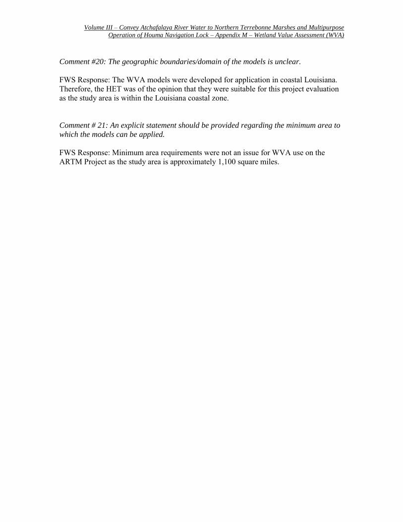
SAND2 Model Verification Verification of the SAND2 model was conducted by simulating the effects of the freshwater diversions (siphons) at Naomi and West Pointe a la Hache, both of which began operating in 1993 (Figure A), and the larger Caernarvon Freshwater Diversion Project, which began operating in 1991. Figure A. Locations of the diversions simulated using the SAND2 model.
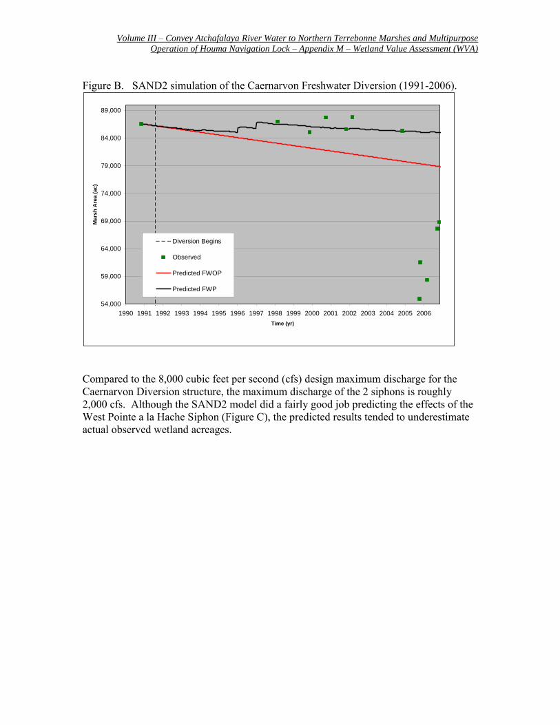
Daily discharge information from each of these diversions was used as input into the SAND2 model. Wetland acreages from the respective influence areas, from 1956 to 1990 were used to determine pre-diversion wetland loss rates. The SAND2 model was then used to predict post-operation wetland acreages. Those predicted acreages were then compared to post-operation observed wetland acreages to verify model results. The SAND2 model did a reasonably good job forecasting Caernarvon benefits until 2005 when Hurricane Katrina caused severe marsh loss in the influence area. Because the model does not incorporate effects of major storm impacts, the model-predicted acreages differed dramatically from observed acreages following Katrina (Figure B).
Volume III – Convey Atchafalaya River Water to Northern Terrebonne Marshes and Multipurpose
Operation of Houma Navigation Lock – Appendix M – Wetland Value Assessment (WVA)
Figure B. SAND2 simulation of the Caernarvon Freshwater Diversion (1991-2006).
Compared to the 8,000 cubic feet per second (cfs) design maximum discharge for the Caernarvon Diversion structure, the maximum discharge of the 2 siphons is roughly 2,000 cfs. Although the SAND2 model did a fairly good job predicting the effects of the West Pointe a la Hache Siphon (Figure C), the predicted results tended to underestimate actual observed wetland acreages.
54,000
59,000
64,000
69,000
74,000
79,000
84,000
89,000
1990 1991 1992 1993 1994 1995 1996 1997 1998 1999 2000 2001 2002 2003 2004 2005 2006
Time (yr)
Mars
h A
rea
(a
c)
Diversion Begins
Observed
Predicted FWOP
Predicted FWP

Volume III – Convey Atchafalaya River Water to Northern Terrebonne Marshes and Multipurpose
Operation of Houma Navigation Lock – Appendix M – Wetland Value Assessment (WVA)
Figure C. SAND2 simulation of the West Pointe a la Hache Siphon (1993-2007).
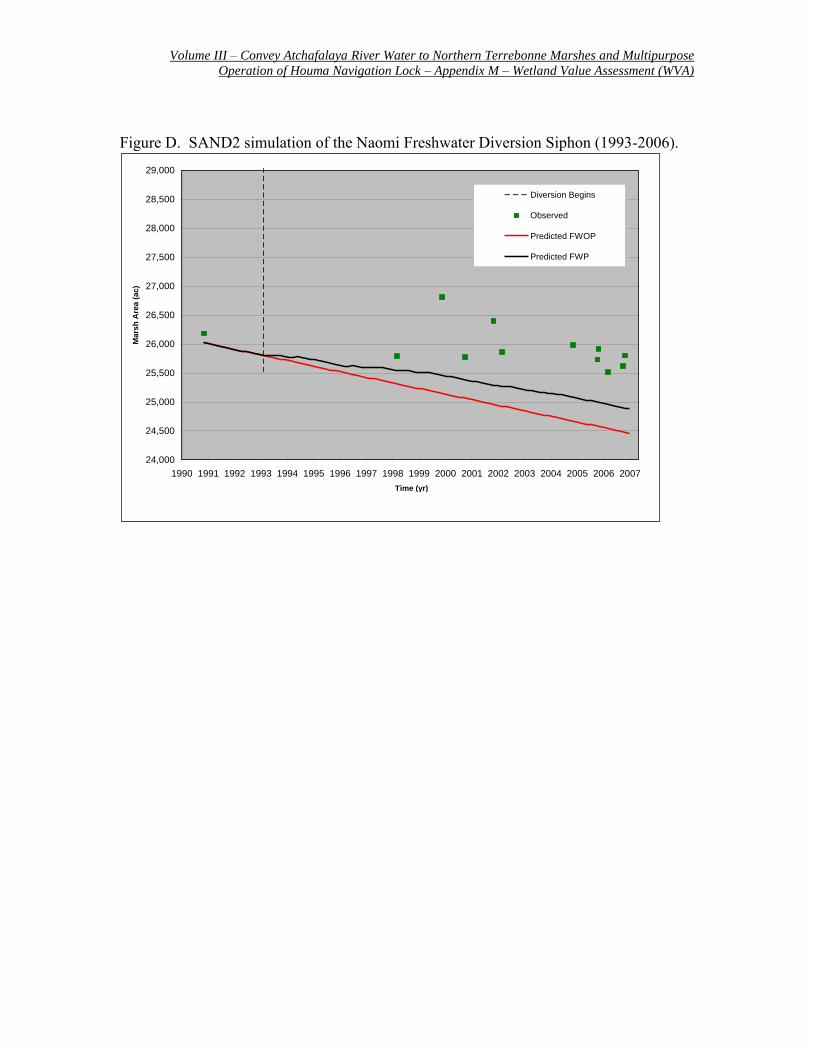
Likewise, the SAND2 results also underestimated wetland acreage in the area influenced by the Naomi Freshwater Diversion Siphon (Figure D). The underestimate for the Naomi Siphon may be related in part to the large and relatively deep open water included within the siphon’s influence area. Exclusion of this area, or a reduction in the influence area size, may have improved the accuracy of model results. This issue highlights the influence of project area selection on model results. Ideally, a hydrologic model or other systematic method to determining the project area (diversion influence area) is needed to achieve the best model results. Unfortunately, there was not sufficient time to conduct model runs to determine the potential ARTM diversion influence areas for each freshwater introduction measure. Instead, influence area polygons were determined using best professional judgment. The SAND2 verification work, and other work with the SAND2 model indicates that it is most applicable in interior marsh systems. When applied to open bays or large lakes, it appears to substantially overestimate land-building. This may be related to resuspension and export of deposited sediments, a process that the model does not address. The ARTM measures, however, are all generally interior locations which are handled well by the SAND2 model. Unfortunately, no examples of freshwater introductions without sediment are available to verify the application of the SAND2 model for nutrient-only situations.
2,000
3,000
4,000
5,000
6,000
7,000
8,000
9,000
10,000
11,000
12,000
13,000
14,000
1990 1991 1992 1993 1994 1995 1996 1997 1998 1999 2000 2001 2002 2003 2004 2005 2006 2007
Time (yr)
Mars
h A
rea
(a
c)
Diversion Begins
Observed
Predicted FWOP
Predicted FWP
Volume III – Convey Atchafalaya River Water to Northern Terrebonne Marshes and Multipurpose
Operation of Houma Navigation Lock – Appendix M – Wetland Value Assessment (WVA)
Figure D. SAND2 simulation of the Naomi Freshwater Diversion Siphon (1993-2006).
24,000
24,500
25,000
25,500
26,000
26,500
27,000
27,500
28,000
28,500
29,000
1990 1991 1992 1993 1994 1995 1996 1997 1998 1999 2000 2001 2002 2003 2004 2005 2006 2007
Time (yr)
Mars
h A
rea
(a
c)
Diversion Begins
Observed
Predicted FWOP
Predicted FWP

Volume III – Convey Atchafalaya River Water to Northern Terrebonne Marshes and Multipurpose
Operation of Houma Navigation Lock – Appendix M – Wetland Value Assessment (WVA)
Annex 3. Quantifying Benefits of Freshwater Flow Diversion to Coastal Marshes:
Theory and Applications.
Quantifying Benefits of Freshwater Flow Diversion to Coastal Marshes: Theorya and Applicationsb
S. Kyle McKay1, J. Craig Fischenich2, S. Jarrell Smith3, and Ronald Paille4
1U.S. Army Engineer Research and Development Center (ERDC) Environmental Laboratory 187 Oglethorpe Ave. Apt. B Athens, Georgia, 30606 Email: [email protected] 2U.S. Army Engineer Research and Development Center (ERDC) Environmental Laboratory 3909 Halls Ferry Rd. Vicksburg, Mississippi, 39180 Email: [email protected] 3U.S. Army Engineer Research and Development Center (ERDC) Coastal and Hydraulics Laboratory 3909 Halls Ferry Rd. Vicksburg, Mississippi, 39180 Email: [email protected] 4U.S. Fish and Wildlife Service 646 Cajundome Boulevard, Suite 400 Lafayette, Louisiana 70506 Email: [email protected] Keywords: wetland, Louisiana, accretion, uncertainty, organic, inorganic, coastal restoration, operation,
Abstract The combination of relative sea level rise and river/marsh disconnection has created a deficit of available soil and accompanying land loss in a large portion of coastal Louisiana. The U.S. Congress recently charged the U.S. Army Corps of Engineers, State of Louisiana, and other federal and local agencies with restoring the coastal wetlands of Louisiana and Mississippi. Many alternative combinations of restoration measures have been proposed, and assessment of the advantages and disadvantages of these efforts must be made to determine the optimal design. One technique being applied for coastal restoration is the reconnection of rivers to coastal marshes through flow diversions.
a Based on material from McKay, S.K., J.C. Fischenich, and S.J. Smith. (2008). “Quantifying Benefits of Flow Diversion to Coastal Marshes. I: Theory.” In draft for submission to Ecological Engineering. b Based on material from McKay, S.K., J.C. Fischenich, and R. Paille. (2008). “Quantifying Benefits of Flow Diversion to Coastal Marshes. II: Application to Louisiana Coastal Protection and Restoration.” In draft for submission to Ecological Engineering.
1
Freshwater flow diversions offer significant nutrient and sediment inputs to marshes that induce both organic and inorganic accumulation of soil. Boustany (2007) presented a screening level model for assessing both the nutrient and sediment benefits of flow diversion over long time scales. This paper has presented the adaptation of Boustany’s (2007) model to include daily variation in sediment processes in order to optimize diversion structure design and operation. The model was verified using an existing diversion to prove the ability of the model to track land evolution associated with flow diversion. This paper also demonstrates the application of the model to diversion operational and structural optimization.
Introduction In the fall of 2005, Hurricanes Katrina and Rita awakened the United States public to the natural protection that coastal wetlands provide in reducing of the effects of hurricanes on coastal communities. In response to these catastrophic events, the U.S. Congress directed the U.S. Army Corps of Engineers (USACE) to “conduct a comprehensive hurricane protection analysis and design…to develop and present a full range of flood control, coastal restoration, and hurricane protection measures” (USACE, 2006). This paper focuses on interagency efforts to assess and weigh benefits of coastal restoration via freshwater flow diversion. The paper will focus on the development and adaptation of a screening level model to quantify the benefits of flow diversion to coastal marshes and will describe the assessment of various diversion operational and structural scenarios.
Coastal Marsh Accretion and Flow Diversion The tidal marshes of coastal Louisiana are receding at alarming rates as high as 115 km2/yr (Barras et al., 1994). Submergence of these valuable ecological assets (Figure 1) was once counteracted by vertical accretion due to the addition of freshwater, nutrient, and mineral inputs from riverine environments; however, eustatic sea level rise (ESLR) and basin subsidence now exceed the current rate of vertical accretion, and coastal marshes have been disconnected from their freshwater and sediment sources, distributary channels of the Mississippi and Atchafalya Rivers. ESLR has been attributed to global increase in ocean volume and has been estimated as 1.0-2.4 mm/yr (Church et al., 2001). Subsidence of the Mississippi delta has been attributed to multiple factors, namely: regional isostasy, faulting, sediment consolidation, and soil dewatering (Dokka et al., 2006). Previous researchers identified other potential sources of subsidence as groundwater and petroleum extraction (Morton et al., 2002); however, Dokka et al. (2006) renounce these hypotheses as unlikely due to the relative lack of groundwater extraction from the highly saltwater intruded groundwater table of most of southern Louisiana and the lack of coincidence between petroleum extraction and subsidence. The synergy of ESLR and basin subsidence has created an apparent local change in sea level known as Relative Sea Level Rise (RSLR) that has been measured in the Mississippi Delta at rates as high as 10 mm/yr (Snedden et al., 2007). In addition to RSLR, the disconnection of coastal marshes from their sediment and nutrient source is equally disconcerting. Over geologic time scales, large-scale delta lobe switching has lead to alternating episodes of delta building and redistribution of sediment
2
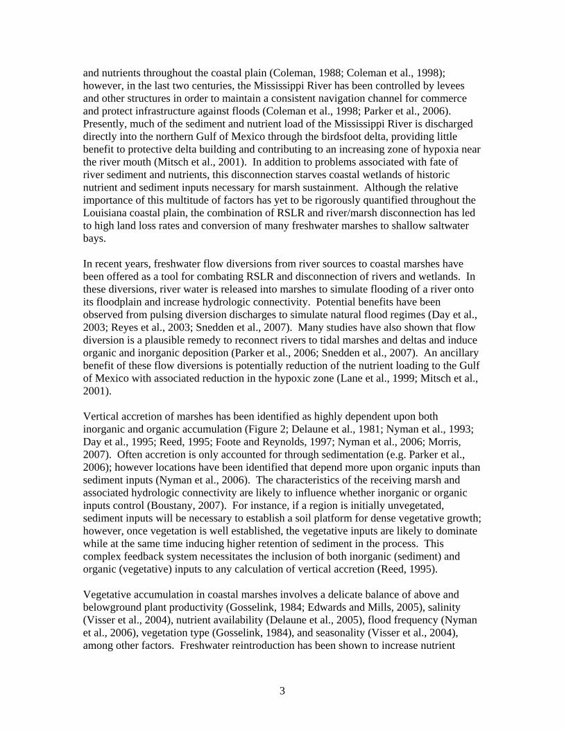
and nutrients throughout the coastal plain (Coleman, 1988; Coleman et al., 1998); however, in the last two centuries, the Mississippi River has been controlled by levees and other structures in order to maintain a consistent navigation channel for commerce and protect infrastructure against floods (Coleman et al., 1998; Parker et al., 2006). Presently, much of the sediment and nutrient load of the Mississippi River is discharged directly into the northern Gulf of Mexico through the birdsfoot delta, providing little benefit to protective delta building and contributing to an increasing zone of hypoxia near the river mouth (Mitsch et al., 2001). In addition to problems associated with fate of river sediment and nutrients, this disconnection starves coastal wetlands of historic nutrient and sediment inputs necessary for marsh sustainment. Although the relative importance of this multitude of factors has yet to be rigorously quantified throughout the Louisiana coastal plain, the combination of RSLR and river/marsh disconnection has led to high land loss rates and conversion of many freshwater marshes to shallow saltwater bays. In recent years, freshwater flow diversions from river sources to coastal marshes have been offered as a tool for combating RSLR and disconnection of rivers and wetlands. In these diversions, river water is released into marshes to simulate flooding of a river onto its floodplain and increase hydrologic connectivity. Potential benefits have been observed from pulsing diversion discharges to simulate natural flood regimes (Day et al., 2003; Reyes et al., 2003; Snedden et al., 2007). Many studies have also shown that flow diversion is a plausible remedy to reconnect rivers to tidal marshes and deltas and induce organic and inorganic deposition (Parker et al., 2006; Snedden et al., 2007). An ancillary benefit of these flow diversions is potentially reduction of the nutrient loading to the Gulf of Mexico with associated reduction in the hypoxic zone (Lane et al., 1999; Mitsch et al., 2001). Vertical accretion of marshes has been identified as highly dependent upon both inorganic and organic accumulation (Figure 2; Delaune et al., 1981; Nyman et al., 1993; Day et al., 1995; Reed, 1995; Foote and Reynolds, 1997; Nyman et al., 2006; Morris, 2007). Often accretion is only accounted for through sedimentation (e.g. Parker et al., 2006); however locations have been identified that depend more upon organic inputs than sediment inputs (Nyman et al., 2006). The characteristics of the receiving marsh and associated hydrologic connectivity are likely to influence whether inorganic or organic inputs control (Boustany, 2007). For instance, if a region is initially unvegetated, sediment inputs will be necessary to establish a soil platform for dense vegetative growth; however, once vegetation is well established, the vegetative inputs are likely to dominate while at the same time inducing higher retention of sediment in the process. This complex feedback system necessitates the inclusion of both inorganic (sediment) and organic (vegetative) inputs to any calculation of vertical accretion (Reed, 1995). Vegetative accumulation in coastal marshes involves a delicate balance of above and belowground plant productivity (Gosselink, 1984; Edwards and Mills, 2005), salinity (Visser et al., 2004), nutrient availability (Delaune et al., 2005), flood frequency (Nyman et al., 2006), vegetation type (Gosselink, 1984), and seasonality (Visser et al., 2004), among other factors. Freshwater reintroduction has been shown to increase nutrient
3
inputs to coastal marshes (Lane et al., 1999) and stimulate growth in these ecosystems (Cardoch et al., 2002), further causing vegetative inputs to contribute to accretion. In coastal Louisiana most marshes are nutrient limited (Nyman et al., 1990; Delaune et al., 2005), so the introduction of limiting nutrients such as nitrogen and phosphorous from flow diversion is a topic of great importance when considering flow diversion alternatives and benefits (Lane et al., 1999; Hyfield, 2004; Hyfield, 2008); however, excessive nutrient loading to coastal wetlands could potentially induce harmful water quality effects such as eutrophication (Delaune et al., 2005) or stimulation of invasive plant species (Carter and Bernard, 2007), so diversion of flow to coastal wetlands must be carefully balanced and planned. The accretion of sediment on coastal marshes and deltas has also been studied extensively (Stumpf, 1983; Wang, 1997; Rybczyk and Cahoon, 2002; Reyes et al., 2003; Parker et al., 2006; Snedden et al., 2007). Relevant sedimentation processes have been identified as sediment loading from floods/diversions (Reed, 1995; Parker et al., 2006), sediment settling properties (Stumpf, 1983; Soulsby, 1997; Winterwerp and van Kesteren, 2004), tidal erosion (Stumpf, 1983; Wang et al., 1997), wind and storm induced erosion and deposition (Wang, 1997), sediment export through canals and bayous (Wang, 1997; Baustian and Turner, 2006), and vegetation induced settling (Gleason et al., 1979; Stumpf, 1983; Reed, 1995; Leonard and Luther, 1995). Although flow diversions have proved useful for combating coastal land loss, the optimization of flow diversion locations and operation has been difficult due to the complexity in data needs of a coupled ecological and hydrodynamic model (Reyes et al., 2003; Delaune et al., 2003; Snedden et al., 2007). These complexities encourage the development of a simple, screening-level model that includes the effects of vegetation and sediment dynamics and allows for straightforward examination and optimization of flow diversion feasibility and operational benefits.
Boustany (2007) Landscape Evolution Model Boustany (2007) developed a composite nutrient and sediment model to assess the feasibility of flow diversions and screen diversion alternatives under the Coastal Wetland Planning, Protection, and Restoration Act (CWPPRA; Boustany, Personal Communication). This model, herein referred to as the Boustany Model (BM), presents all benefits of flow diversion in terms of marsh area by assuming all nutrient and sediment benefits additive to the existing area and land change rate:
sedinutii AAAA ++=+ δ1 Equation 1 Where Ai is the marsh area at time i, δnut is the fractional change in land area due to RSLR and river-marsh disconnection (value may be positive or negative) that has been adjusted to account for the benefits associated with nutrient addition, and Ased is the area benefit of sediment addition. The BM was developed to compare long term relative benefits of many flow diversion locations and was implemented with an annual time step to provide quick estimates of the potential benefits of diversions. The BM is sufficient for quick estimation of flow
4
diversion benefits and initial screening of alternatives, but the LACPR program required greater temporal resolution in order to assess not only the relative benefits of diversion locations, but also the effects of diversion structure type, diversion operational regimes, and hydrologic variability. Ideally a detailed two- or three-dimensional model coupling nutrient and sediment processes would be used to account for the complex mechanisms governing coastal marsh accretion (Reyes et al., 2000; Dortch et al., 2007); however, the vast number of alternatives and short time scale of the LACPR report to Congress precluded development of such models for every alternative and marsh. As such, the BM was adapted to include processes deemed most critical to LACPR alternatives analysis. The following sections provide further details of the nutrient and sediment models implemented in the landscape evolution calculations, but the two major adaptations of the BM were:
• High temporal variability in sediment processes encouraged the refinement of the temporal resolution of the sediment model to include daily impacts of the diversion on the marsh.
• In order to maintain model simplicity, the BM required estimation of a number of parameters to account for nutrient and sediment processes (e.g. sediment retention and average annual suspended sediment concentration). The adaptation of the model has also included the calculation of many of these inputs in order to account for temporal variance, reduce data requirements, and minimize potential input errors.
Nutrient Benefits Nutrient addition to coastal marshes has proven to be a source of vegetation stimulation and strengthening and biomass creation (Deegan et al., 2007). Boustany (2007) proposes a model that accounts for the ability of nutrients to stimulate vegetation to better resist erosional processes. This model determines the percent of the vegetated area that is strengthened from nutrient addition. This parameter is found by examining the annual nutrient requirements of the marsh relative to the nutrients loaded to the marsh. The nutrients required by the marsh for vegetative growth are assumed to be the mass of the nutrients held in plant biomass. This quantity may be assessed by examining the rate of biomass production (annual primary productivity, Pr) and the percent of biomass containing these nutrients (γ). Since most Louisiana coastal marshes are nitrogen or phosphorous limited, Boustany proposes that the total concentration of nitrogen and phosphorous (TNP) be used to account for nutrient benefits.
TNPrreq PLR γ= Equation 2 Where LRreq is the marsh required nutrient loading rate [ML-2T-1], Pr is primary productivity [ML-2T-1], and γTNP is the percent of plant biomass containing nitrogen and phosphorous [1]. The nutrient loading rate of the diversion to plant biomass, LRdiv, may be calculated from the volumetric discharge of water to the marsh from the diversion, Qdiv [L3T-1], the
5
concentration of nutrients in the source water, Csource [ML-3], the retention rate of nutrients in plant biomass, Rnut [1], and the vegetated marsh area, Aveg [L2].
nutveg
sourcedivdiv R
ACQ
LR =
Equation 3 In addition to nutrient loading from the diversion, there is ambient nutrient loading to the marsh from other ongoing processes (e.g. atmospheric deposition, stormwater runoff, current plant decomposition, denitrification, etc.). These processes will be accounted for by a loading rate for background sources, LRbackground. The net loading of nutrients to the marsh, LRnet, is therefore the sum of the background and diversion loading rates.
backgrounddivnet LRLRLR += Equation 4 From knowledge of the loading rates applied, LRnet, and required, LRreq, one may obtain the fraction of wetlands sustained by nutrient addition, Es.
req
nets LR
LRE =
Equation 5 In this model, nutrients are assumed to be unable to freely construct land; however, they can reduce the loss rate by strengthening vegetated areas against erosion. This assumption produces conservative estimates of the organically-induced benefits of the diversion. For instance, in an environment with a low land loss rate, according to the model, the diversion could potentially reduce the land loss to zero; however, no land gain would be associated with organic inputs. The percentage of wetland sustained by nutrient addition serves as a reduction ratio to the land loss rate in the form of Equation 6.
( )⎩⎨⎧
≥<−
=1011
s
ssnut ForE
ForEEδδ
Equation 6 Where δ is the land change rate prior to the diversion and δnut is the nutrient adjusted land change rate.
Sediment Benefits The accumulation of diverted sediments is determined by a sediment budgeting model utilizing the input concentration of sediment from the source water and calculated hydrodynamics of the system to determine the quantity of diverted sediment retained in the marsh. As previously specified, the BM implemented sedimentation calculations on an annual timescale, and while this assumption is reasonable for preliminary screening of alternatives, further refinement is necessary for more detailed analyses of flow diversion benefits. The sediment model implemented herein relies on calculation of sediment inputs and sediment settling theory on a daily timescale over a single representative year and reapplies that year throughout the proposed project life cycle.
Sediment Input In order to minimize costs and maximize benefits of flow diversion in coastal Louisiana, diversion structures often withdraw water from one of the region’s major rivers (e.g.
6
Mississippi, Atchafalya, Calcasieu). These rivers are located throughout the coastal plain, carry large water and sediment loads, and serve as a virtually infinite source of diversion resources. River discharge and suspended sediment concentration have often been shown to be positively correlated (Mossa, 1996; Snedden et al., 2007). The relationship between discharge and sediment load may be determined by analytical and partially analytical models (e.g. Meyer-Peter Muller, Einstein, Yang; Richardson et al., 2001) or by empirical models for a given set of observed discharge and sediment concentration values (Mossa, 1996; Snedden et al., 2007). In coastal Louisiana, there exists enough recorded sediment discharge data to generate empirical models of sediment concentration for some of the major rivers of the region. For this analysis, a power function was found to provide enough resolution in sediment concentration variation (Equation 7). Table 1 presents a number of sediment ratings of this form for coastal Louisiana.
21,
ariverrivers QaQ =
Equation 7 Where Qs,river is sediment load (ton/da), Qriver is river discharge (cfs), a1 is a dimensional coefficient, and a2 is a dimensionless coefficient. From this sediment rating, flow-averaged suspended sediment concentration of the river, Criver, may be
calculated ⎟⎠⎞
⎜⎝⎛ =
river
riversriver Q
QC , and transformed to the desired units.
Regardless of the model defining this relationship, the sediment concentration has been shown to be highly dependent upon discharge; therefore, in order to capture the temporal variance in sediment discharge through a diversion, the sediment concentration must vary with river discharge at an appropriate time scale (Snedden et al., 2007). For the purposes of this analysis, daily variation in discharge provides sufficient temporal resolution for accurate calculation of sediment loading to marshes by diversions. One of the purposes for adapting the BM is the desire to examine relative diversion structure operation. In order to do this, daily estimates of diversion discharge are also required. These daily diversion discharges, Qdiv, are combined with the daily predictions of river suspended sediment concentration, Criver, to determine the mass loading rate of sediment to the marsh, Qs,div (Equation 8). This increase in temporal resolution allows for examination of diversion discharge operation such that sediment benefits may be maximized by coinciding diversion discharges with periods of high river suspended sediment concentration.
riverdivdivs CQQ =, Equation 8
Sediment Retention After sediment laden water has been diverted to a coastal wetland, a portion of the sediment load is expected to settle from suspension and deposit. Sediment that remains in suspension is then subject to being transported outside the system boundaries. Sediment retention defines the fraction of diverted sediments retained within the coastal wetland.
7
Retention is dependent upon system properties such as: wetland geometry, diversion discharge, tidal velocities (Stumpf, 1983), wind and storm events (Wang, 1997), settling velocity of diverted sediments (Soulsby, 1997; Winterwerp and van Kesteren, 2004), vegetation coverage (Stumpf, 1983), and canal-induced sediment import/export (Wang, 1997). The approach taken by Boustany (2007) is to apply retention factors estimated for other sites (e.g. Wax Lake Outlet) or allow the analyst to choose a retention factor based on knowledge of the receiving area and best professional judgment. Building upon the suggestion of Stumpf (1983), an alternative to this approach is to use a simple calculation which includes effects of wetland geometry, sediment properties, and flow hydrodynamics at the site. The effects of vegetation and channels are ignored in this analysis in order to maintain model simplicity; however, vegetation would likely increase roughness, reduce turbulence, and induce greater sediment deposition leading to conservatively low estimates of sediment retention, while the influence of channels may serve as pathways to sediment export and thus produce non-conservatively high estimates of sediment retention. Consider suspended sediments in a water body. The time required for a given particle to settle from the water surface to the bed is given as:
effsWHT
,
=
Equation 9 Where T is the time required for sediment to completely settle, H is the local depth, and Ws,eff is the effective settling velocity of a specific sediment class. As the particle settles, it is also transported by tidal and diversion currents, so the distance traveled by the particle is:
effsdivdiv W
HUTUX,
==
Equation 10 Where U is the diversion induced mean velocity. As the averaging timescale of the model is greater than the tidal period and net tidal flow is zero, Equation 10 neglects the influence of tidal velocities, and the net displacement of water within the marsh is described by the diversion flow. For this analysis the wetland is assumed to have rectangular planform and cross-sectional geometries described by the average length (L), width (B), and depth (H). The fraction of sediment retained in the wetland then becomes a function of wetland length relative to transport distance prior to full deposition of the sediment fraction in question (Stumpf, 1983). If all diverted sediment is retained within the system, the retention factor is 1. Since this analysis takes a macroscopic view of the total sediment retained in the system and location of deposit is not considered, the retention factor becomes 1 if the length of the wetland is greater than the transport length, and the retention of a given sediment particle class, Rj, may be expressed as:
⎟⎠⎞
⎜⎝⎛= 1,min
XLR j
8

Equation 11 Due to variation in fall velocity with sediment size, coarse particles may be retained while fines are flushed from the system; therefore, the combined retention of the entire grain size distribution must be made. Retention over all sediment classes may be expressed as:
∑= jjT fRR Equation 12 Where RT is the combined total retention factor and fj is the mass fraction associated with each sediment class.
Fall Velocity A key element of the sediment budgeting model presented is the calculation of the effective fall velocity of a given sediment size class, which is a function of the fall velocity of that sediment in a static body of water, Ws, and the turbulence of the flow. Fall velocity of sediment is dependent upon both sediment properties (shape, size, density, concentration, ability to flocculate) and fluid properties (viscosity, density, temperature, salinity). In the natural environment, turbulence is generated by flow over the sediment bed. The presence of turbulence acts to vertically mix suspended sediments, which reduces the effective settling velocity of suspended particles. The steady-state vertical flux balance at a point in the water column is given by:
0=+dzdCKCW zs
Equation 13 Where C is the suspended sediment concentration, Kz is the vertical diffusivity, and z is the vertical distance from the bed. For the purposes of this tool to estimate retention, it is convenient to combine the terms in Equation 13 to define an effective settling velocity (Equation 14).
dzdCKCWCW zseffs +=,
Equation 14 Vertical diffusivity varies with turbulent intensity and height above the bed. Rouse proposes that diffusivity varies parabolically with height above the bed in the form (Richardson et al., 2001):
⎟⎠⎞
⎜⎝⎛ −=
HzzuK z 1*κ
Equation 15 Where κ is the von Karman constant (~0.4) and u* is the total friction velocity (a measure of turbulent intensity). Given the sediment flux balance in Equation 13, the vertical concentration profile is:
b
a
aa zH
zHzzCC
−
⎟⎟⎠
⎞⎜⎜⎝
⎛−−
=
Equation 16
9
Where b is the Rouse parameter ⎟⎠⎞⎜
⎝⎛ =
*uWb s
κ and za is a reference height above the bed
with a known sediment condition, Ca. The turbulent shear velocity is estimated from the depth-averaged velocity by the logarithmic boundary layer (law of the wall) (Kundu, 1990).
⎟⎟⎟
⎠
⎞
⎜⎜⎜
⎝
⎛=
0
*
3lnz
HUu κ
Equation 17 Where U is the daily mean wetland velocity with both tidal and diversion related components and z0 is the hydraulic roughness length. For the diurnal tidal cycle of coastal Louisiana, the tide is assumed to have approximately sinusoidal periodicity. The mean instantaneous wetland velocity can then be determined by considering both tidal and diversion components (Figure 3).
ωω sinsin max,max, tidediv
tidedivi UHBQ
UUU +=+=
Equation 18 Where Ui is the instantaneous mean velocity with tidal and diversion components and Umax,tide is the maximum tidal velocity (or tidal amplitude), and ω is tide phase. For the use in the flow diversion model, the velocity is integrated over the tidal cycle (0 to 2π) to obtain the daily mean velocity, U.
( ) ( ) ( )( ){ }012max,201 coscos2cos221 ωωωωωωπ
+−+−−= tidediv UUU ( )
Equation 19
Where ω0 is the tide phase at zero up-crossing ⎟⎠
⎞⎜⎝
⎛⎟⎠⎞
⎜⎝⎛−= −
tide
divU
Umax,
10 sinω , ω1 is the tide
phase at zero down-crossing ( )01 ωπω −= , and ω2 is the completed tidal phase ( )πωω 202 += (Figure 3). In order to estimate the shear velocity, the hydraulic roughness must also be estimated from local sediment grain size, form roughness, and vegetative coverage. In this analysis, a lumped parameter accounting for both grain size and form roughness is implemented based on marsh surface character (Table 2). Vegetative roughness is incredibly important in coastal marshes where emergent plants are encountered throughout the marsh, and although basing this parameter on bed material ignores the effects of vegetation, this will provide an estimate of sediment settling in open water and will therefore provide conservative estimates of settling in vegetated or partially vegetated marsh.
10
Combining Equation 13 – Equation 17, one may obtain an expression for the effective settling velocity of sediment in coastal marshes.
( ) ⎟⎟⎠
⎞⎜⎜⎝
⎛
−⎟⎠⎞
⎜⎝⎛
−⎟⎟⎠
⎞⎜⎜⎝
⎛ −−=
−−−
2
1
, zHH
zHz
zzH
bKWWbb
a
azseffs
Equation 20 For incorporation into the flow diversion model, vertical mixing has been computed at a height above the bed equal to 1/10 of water depth ( )10
Hz = and za is approximated as
1/100 of the depth ( )100Hza = . These values provide an estimate of the settling velocity
of particles very near the bed that are assumed to settle. Insertion of these relations into Equation 20 yields:
( ) ⎟⎠⎞
⎜⎝⎛
⎟⎠⎞
⎜⎝⎛−=
−−−
HbKWW
bb
zseffs81.0
9199
1
,
Equation 21 Where HuK z *009.0 κ= .
Net Sediment Benefit By accounting for sediment loading to the marsh and sediment retention within the marsh, the mass loading rate of sediment retained in the marsh may be determined by:
Tdivsnets RQQ ,, = Equation 22 Where Qs,net is the net mass loading rate of sediment to the marsh. This loading rate may then be used to calculate the net aerial sediment benefit due to flow diversion, Ased, for a given time period.
bd
netssed H
dtQA
ρ,=
Equation 23 Where dt is the time step (da) and ρbd is the average bulk density of the receiving area. Bulk density in coastal marshes varies significantly with depth due to sediment consolidation. For our analysis, we assumed that the bulk density was a depth averaged value based on the depth of marsh being filled with sediment (i.e. flow depth, H). Bulk density profiles were obtained from literature (Nyman et al., 1990; Nyman et al., 1993; Delaune et al., 2003) and available data (Michael Channel, personal communication).
Application: Caernarvon Diversion and Breton Sound Estuary In order to verify the ability of the model to account for landscape evolution due to flow diversion, the model was applied to an existing diversion structure and marsh, the Caernarvon Diversion to Upper Breton Sound Estuary (Figure 4). The Caernarvon Diversion is located on the east bank of the Mississippi River at river mile 81.5 (131.2 km) (approximately 12.5 river miles (20.1 km) downstream of New Orleans) and
11
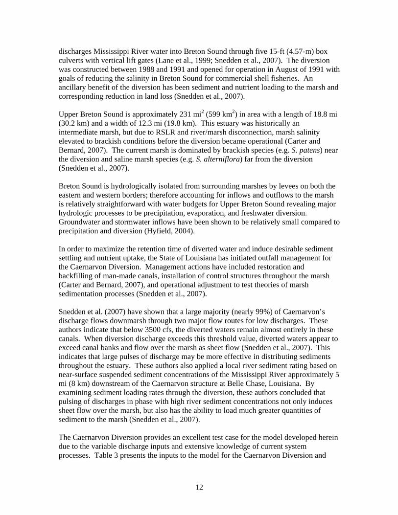
discharges Mississippi River water into Breton Sound through five 15-ft (4.57-m) box culverts with vertical lift gates (Lane et al., 1999; Snedden et al., 2007). The diversion was constructed between 1988 and 1991 and opened for operation in August of 1991 with goals of reducing the salinity in Breton Sound for commercial shell fisheries. An ancillary benefit of the diversion has been sediment and nutrient loading to the marsh and corresponding reduction in land loss (Snedden et al., 2007). Upper Breton Sound is approximately 231 mi2 (599 km2) in area with a length of 18.8 mi (30.2 km) and a width of 12.3 mi (19.8 km). This estuary was historically an intermediate marsh, but due to RSLR and river/marsh disconnection, marsh salinity elevated to brackish conditions before the diversion became operational (Carter and Bernard, 2007). The current marsh is dominated by brackish species (e.g. S. patens) near the diversion and saline marsh species (e.g. S. alterniflora) far from the diversion (Snedden et al., 2007). Breton Sound is hydrologically isolated from surrounding marshes by levees on both the eastern and western borders; therefore accounting for inflows and outflows to the marsh is relatively straightforward with water budgets for Upper Breton Sound revealing major hydrologic processes to be precipitation, evaporation, and freshwater diversion. Groundwater and stormwater inflows have been shown to be relatively small compared to precipitation and diversion (Hyfield, 2004). In order to maximize the retention time of diverted water and induce desirable sediment settling and nutrient uptake, the State of Louisiana has initiated outfall management for the Caernarvon Diversion. Management actions have included restoration and backfilling of man-made canals, installation of control structures throughout the marsh (Carter and Bernard, 2007), and operational adjustment to test theories of marsh sedimentation processes (Snedden et al., 2007). Snedden et al. (2007) have shown that a large majority (nearly 99%) of Caernarvon’s discharge flows downmarsh through two major flow routes for low discharges. These authors indicate that below 3500 cfs, the diverted waters remain almost entirely in these canals. When diversion discharge exceeds this threshold value, diverted waters appear to exceed canal banks and flow over the marsh as sheet flow (Snedden et al., 2007). This indicates that large pulses of discharge may be more effective in distributing sediments throughout the estuary. These authors also applied a local river sediment rating based on near-surface suspended sediment concentrations of the Mississippi River approximately 5 mi (8 km) downstream of the Caernarvon structure at Belle Chase, Louisiana. By examining sediment loading rates through the diversion, these authors concluded that pulsing of discharges in phase with high river sediment concentrations not only induces sheet flow over the marsh, but also has the ability to load much greater quantities of sediment to the marsh (Snedden et al., 2007). The Caernarvon Diversion provides an excellent test case for the model developed herein due to the variable discharge inputs and extensive knowledge of current system processes. Table 3 presents the inputs to the model for the Caernarvon Diversion and
12
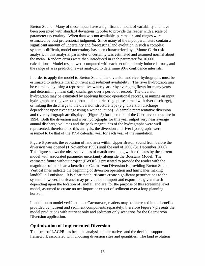
Breton Sound. Many of these inputs have a significant amount of variability and have been presented with standard deviations in order to provide the reader with a scale of parameter uncertainty. When data was not available, parameters and ranges were estimated by best professional judgment. Since many of the input parameters contain a significant amount of uncertainty and forecasting land evolution in such a complex system is difficult, model uncertainty has been characterized by a Monte Carlo risk analysis. In this analysis, parameter uncertainty was estimated and assumed normal about the mean. Random errors were then introduced in each parameter for 10,000 calculations. Model results were computed with each set of randomly induced errors, and the range of area predictions was analyzed to determine 90% confidence intervals. In order to apply the model to Breton Sound, the diversion and river hydrographs must be estimated to indicate marsh nutrient and sediment availability. The river hydrograph may be estimated by using a representative water year or by averaging flows for many years and determining mean daily discharges over a period of record. The diversion hydrograph may be estimated by applying historic operational records, assuming an input hydrograph, testing various operational theories (e.g. pulses timed with river discharge), or linking the discharge to the diversion structure type (e.g. diversion discharge dependence upon river stage using a weir equation). A sample representative diversion and river hydrograph are displayed (Figure 5) for operation of the Caernarvon structure in 1994. Both the diversion and river hydrographs for this year output very near average annual discharge volumes and the peak magnitudes of the hydrographs were well represented; therefore, for this analysis, the diversion and river hydrographs were assumed to be that of the 1994 calendar year for each year of the simulation. Figure 6 presents the evolution of land area within Upper Breton Sound from before the diversion was opened (1 November 1990) until the end of 2006 (31 December 2006). This figure shows the observed values of marsh area along with estimates by the current model with associated parameter uncertainty alongside the Boustany Model. The estimated future without project (FWOP) is presented to provide the reader with the magnitude of marsh area benefit the Caernarvon Diversion is providing Breton Sound. Vertical lines indicate the beginning of diversion operation and hurricanes making landfall in Louisiana. It is clear that hurricanes create significant perturbations to the system; however, hurricanes may provide both import and export to a given marsh depending upon the location of landfall and are, for the purpose of this screening level model, assumed to create no net import or export of sediment over a long planning horizon. In addition to model verification at Caernarvon, readers may be interested in the benefits provided by nutrient and sediment components separately; therefore Figure 7 presents the model predictions with nutrient only and sediment only scenarios for the Caernarvon Diversion application.
Optimization of Implemented Diversion The focus of LACPR has been the analysis of alternatives and the decision support framework associated with choosing diversion sites and quantities. The land evolution
13
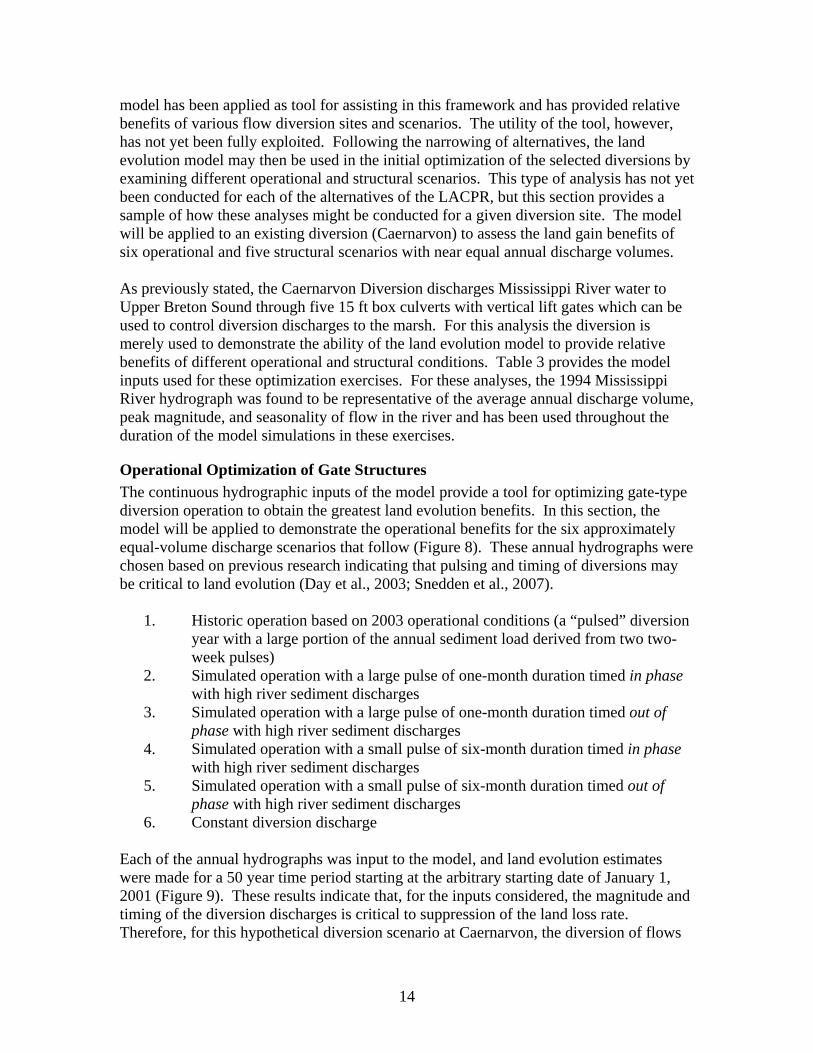
model has been applied as tool for assisting in this framework and has provided relative benefits of various flow diversion sites and scenarios. The utility of the tool, however, has not yet been fully exploited. Following the narrowing of alternatives, the land evolution model may then be used in the initial optimization of the selected diversions by examining different operational and structural scenarios. This type of analysis has not yet been conducted for each of the alternatives of the LACPR, but this section provides a sample of how these analyses might be conducted for a given diversion site. The model will be applied to an existing diversion (Caernarvon) to assess the land gain benefits of six operational and five structural scenarios with near equal annual discharge volumes. As previously stated, the Caernarvon Diversion discharges Mississippi River water to Upper Breton Sound through five 15 ft box culverts with vertical lift gates which can be used to control diversion discharges to the marsh. For this analysis the diversion is merely used to demonstrate the ability of the land evolution model to provide relative benefits of different operational and structural conditions. Table 3 provides the model inputs used for these optimization exercises. For these analyses, the 1994 Mississippi River hydrograph was found to be representative of the average annual discharge volume, peak magnitude, and seasonality of flow in the river and has been used throughout the duration of the model simulations in these exercises.
Operational Optimization of Gate Structures The continuous hydrographic inputs of the model provide a tool for optimizing gate-type diversion operation to obtain the greatest land evolution benefits. In this section, the model will be applied to demonstrate the operational benefits for the six approximately equal-volume discharge scenarios that follow (Figure 8). These annual hydrographs were chosen based on previous research indicating that pulsing and timing of diversions may be critical to land evolution (Day et al., 2003; Snedden et al., 2007).
1. Historic operation based on 2003 operational conditions (a “pulsed” diversion year with a large portion of the annual sediment load derived from two two-week pulses)
2. Simulated operation with a large pulse of one-month duration timed in phase with high river sediment discharges
3. Simulated operation with a large pulse of one-month duration timed out of phase with high river sediment discharges
4. Simulated operation with a small pulse of six-month duration timed in phase with high river sediment discharges
5. Simulated operation with a small pulse of six-month duration timed out of phase with high river sediment discharges
6. Constant diversion discharge Each of the annual hydrographs was input to the model, and land evolution estimates were made for a 50 year time period starting at the arbitrary starting date of January 1, 2001 (Figure 9). These results indicate that, for the inputs considered, the magnitude and timing of the diversion discharges is critical to suppression of the land loss rate. Therefore, for this hypothetical diversion scenario at Caernarvon, the diversion of flows
14

could be altered to be in phase with high river sediment discharges and should occur from later winter to early summer (February – June). These periods of high sediment discharge may not, however, align with other project goals of a given diversion (e.g. reduction of salinity for maintenance of commercial fisheries). This analysis indicates a time period over which the greatest land evolution benefits may be obtained, and diversion operation may be optimized within that timeframe to include multiple project goals.
Structure Selection Not only will operational considerations impact diversion benefits, but structure type will also have a drastic impact on the selection and operation of a given diversion. For instance, a gate-type structure (such as the one at Caernarvon) may be controlled to achieve the desired water and sediment discharges, but the cost and maintenance may be high. Whereas a broad-crested weir may have low cost, but control of diversion discharges is relatively minimal. A siphon is a third common diversion structure that may require significant maintenance and operational effort, but the suspended sediment concentration of the diverted water may be higher and the size gradation of the sediment diverted may be significantly larger inducing more land gain on both accounts. This section will demonstrate the ability of the model to assess land evolution by applying the model to the Caernarvon Diversion for the following five hypothetical structural scenarios:
1. Gate structure with pulsed operation based on the 2003 hydrograph 2. 100-ft wide broad-crested weir 3. 200-ft wide broad-crested weir structure 4. 1 – 15 ft siphon with a single short duration (113 day) discharge event 5. 1 – 6 ft siphon with continuous operation throughout the year
The weir structures have been assumed to behave as theoretical broad-crested weirs (Equation 24) and the discharge was determined based on the Mississippi River stage for the representative hydrograph (1994). The weir elevations were adjusted to produce annual discharge volumes approximately equal to the average annual diversion discharge volume from 1991-2006.
( ) 2/3weirriverweirweirdiv zzBCQ −=
Equation 24 Where Cweir is a weir coefficient (~4.37 ft0.5/s), BBweir is the width of the weir (ft), zriver is the elevation of the river for a given flow rate (ft), zweir is the elevation of the weir (ft) (White, 2003). In order to calculate the discharge of the diversion by siphoning, Bernoulli’s equation was implemented (Equation 25). Frictional losses in the pipe were assumed negligible due to the qualitative nature of this analysis. As with the weir, the marsh elevation was optimized to produce annual discharge volumes approximately equal to the average annual diversion discharge volume from 1991-2006. Figure 10 presents diversion discharge hydrographs for the five scenarios considered.
15
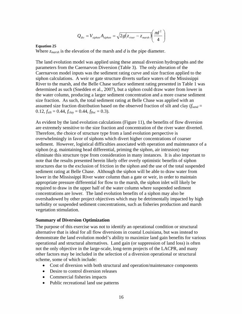
( ) ⎟⎟⎠
⎞⎜⎜⎝
⎛−==
42
2dzzgAVQ marshriversiphonsiphondivπ
Equation 25 Where zmarsh is the elevation of the marsh and d is the pipe diameter. The land evolution model was applied using these annual diversion hydrographs and the parameters from the Caernarvon Diversion (Table 3). The only alteration of the Caernarvon model inputs was the sediment rating curve and size fraction applied to the siphon calculations. A weir or gate structure diverts surface waters of the Mississippi River to the marsh, and the Belle Chase surface sediment rating presented in Table 1 was determined as such (Snedden et al., 2007), but a siphon could draw water from lower in the water column, producing a larger sediment concentration and a more coarse sediment size fraction. As such, the total sediment rating at Belle Chase was applied with an assumed size fraction distribution based on the observed fraction of silt and clay (fsand = 0.12, fsilt = 0.44, fclay = 0.44, ffloc = 0.3). As evident by the land evolution calculations (Figure 11), the benefits of flow diversion are extremely sensitive to the size fraction and concentration of the river water diverted. Therefore, the choice of structure type from a land evolution perspective is overwhelmingly in favor of siphons which divert higher concentrations of coarser sediment. However, logistical difficulties associated with operation and maintenance of a siphon (e.g. maintaining head differential, priming the siphon, air intrusion) may eliminate this structure type from consideration in many instances. It is also important to note that the results presented herein likely offer overly optimistic benefits of siphon structures due to the exclusion of friction in the siphon and the use of the total suspended sediment rating at Belle Chase. Although the siphon will be able to draw water from lower in the Mississippi River water column than a gate or weir, in order to maintain appropriate pressure differential for flow to the marsh, the siphon inlet will likely be required to draw in the upper half of the water column where suspended sediment concentrations are lower. The land evolution benefits of a siphon may also be overshadowed by other project objectives which may be detrimentally impacted by high turbidity or suspended sediment concentrations, such as fisheries production and marsh vegetation stimulation.
Summary of Diversion Optimization The purpose of this exercise was not to identify an operational condition or structural alternative that is ideal for all flow diversions in coastal Louisiana, but was instead to demonstrate the land evolution model’s ability to maximize land gain benefits for various operational and structural alternatives. Land gain (or suppression of land loss) is often not the only objective in the large-scale, long-term projects of the LACPR, and many other factors may be included in the selection of a diversion operational or structural scheme, some of which include:
• Cost of diversion with both structural and operation/maintenance components • Desire to control diversion releases • Commercial fisheries impacts • Public recreational land use patterns
16
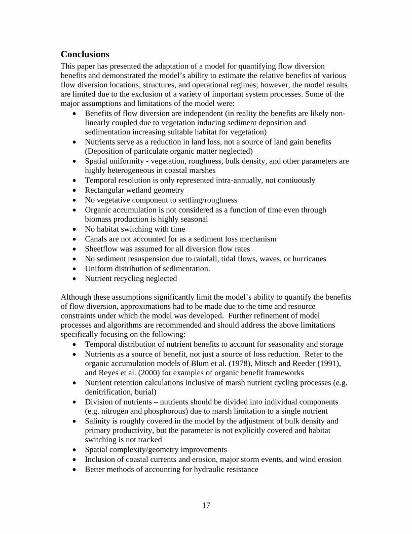
Conclusions This paper has presented the adaptation of a model for quantifying flow diversion benefits and demonstrated the model’s ability to estimate the relative benefits of various flow diversion locations, structures, and operational regimes; however, the model results are limited due to the exclusion of a variety of important system processes. Some of the major assumptions and limitations of the model were:
• Benefits of flow diversion are independent (in reality the benefits are likely non-linearly coupled due to vegetation inducing sediment deposition and sedimentation increasing suitable habitat for vegetation)
• Nutrients serve as a reduction in land loss, not a source of land gain benefits (Deposition of particulate organic matter neglected)
• Spatial uniformity - vegetation, roughness, bulk density, and other parameters are highly heterogeneous in coastal marshes
• Temporal resolution is only represented intra-annually, not contiuously • Rectangular wetland geometry • No vegetative component to settling/roughness • Organic accumulation is not considered as a function of time even through
biomass production is highly seasonal • No habitat switching with time • Canals are not accounted for as a sediment loss mechanism • Sheetflow was assumed for all diversion flow rates • No sediment resuspension due to rainfall, tidal flows, waves, or hurricanes • Uniform distribution of sedimentation. • Nutrient recycling neglected
Although these assumptions significantly limit the model’s ability to quantify the benefits of flow diversion, approximations had to be made due to the time and resource constraints under which the model was developed. Further refinement of model processes and algorithms are recommended and should address the above limitations specifically focusing on the following:
• Temporal distribution of nutrient benefits to account for seasonality and storage • Nutrients as a source of benefit, not just a source of loss reduction. Refer to the
organic accumulation models of Blum et al. (1978), Mitsch and Reeder (1991), and Reyes et al. (2000) for examples of organic benefit frameworks
• Nutrient retention calculations inclusive of marsh nutrient cycling processes (e.g. denitrification, burial)
• Division of nutrients – nutrients should be divided into individual components (e.g. nitrogen and phosphorous) due to marsh limitation to a single nutrient
• Salinity is roughly covered in the model by the adjustment of bulk density and primary productivity, but the parameter is not explicitly covered and habitat switching is not tracked
• Spatial complexity/geometry improvements • Inclusion of coastal currents and erosion, major storm events, and wind erosion • Better methods of accounting for hydraulic resistance
17
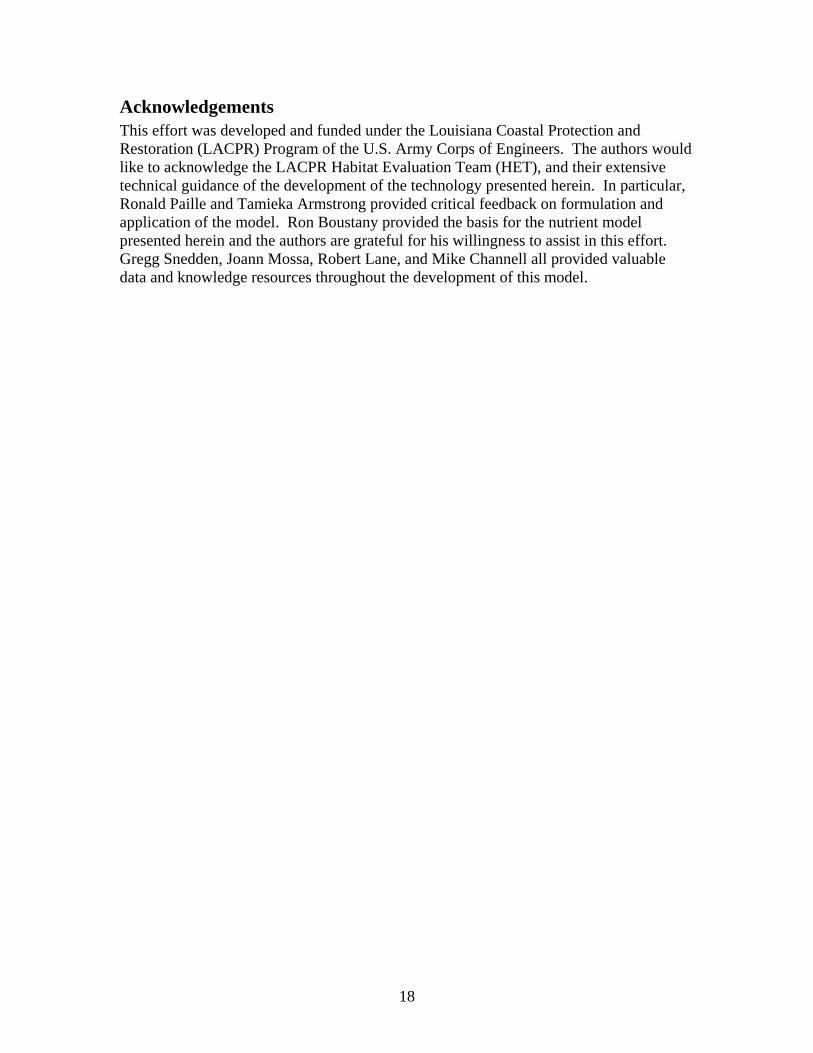
Acknowledgements This effort was developed and funded under the Louisiana Coastal Protection and Restoration (LACPR) Program of the U.S. Army Corps of Engineers. The authors would like to acknowledge the LACPR Habitat Evaluation Team (HET), and their extensive technical guidance of the development of the technology presented herein. In particular, Ronald Paille and Tamieka Armstrong provided critical feedback on formulation and application of the model. Ron Boustany provided the basis for the nutrient model presented herein and the authors are grateful for his willingness to assist in this effort. Gregg Snedden, Joann Mossa, Robert Lane, and Mike Channell all provided valuable data and knowledge resources throughout the development of this model.
18
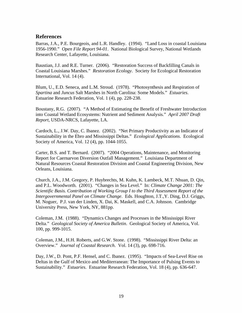
References Barras, J.A., P.E. Bourgeois, and L.R. Handley. (1994). “Land Loss in coastal Louisiana 1956-1990.” Open File Report 94-01. National Biological Survey, National Wetlands Research Center, Lafayette, Louisiana. Baustian, J.J. and R.E. Turner. (2006). “Restoration Success of Backfilling Canals in Coastal Louisiana Marshes.” Restoration Ecology. Society for Ecological Restoration International, Vol. 14 (4). Blum, U., E.D. Seneca, and L.M. Stroud. (1978). “Photosynthesis and Respiration of Spartina and Juncus Salt Marshes in North Carolina: Some Models.” Estuaries. Estuarine Research Federation, Vol. 1 (4), pp. 228-238. Boustany, R.G. (2007). “A Method of Estimating the Benefit of Freshwater Introduction into Coastal Wetland Ecosystems: Nutrient and Sediment Analysis.” April 2007 Draft Report, USDA-NRCS, Lafayette, LA. Cardoch, L., J.W. Day, C. Ibanez. (2002). “Net Primary Productivity as an Indicator of Sustainability in the Ebro and Mississippi Deltas.” Ecological Applications. Ecological Society of America, Vol. 12 (4), pp. 1044-1055. Carter, B.S. and T. Bernard. (2007). “2004 Operations, Maintenance, and Monitoring Report for Caernarvon Diversion Outfall Management.” Louisiana Department of Natural Resources Coastal Restoration Division and Coastal Engineering Division, New Orleans, Louisiana. Church, J.A., J.M. Gregory, P. Huybrechts, M. Kuhn, K. Lambeck, M.T. Nhuan, D. Qin, and P.L. Woodworth. (2001). “Changes in Sea Level.” In: Climate Change 2001: The Scientific Basis. Contribution of Working Group I to the Third Assessment Report of the Intergovernmental Panel on Climate Change. Eds. Houghton, J.T.,Y. Ding, D.J. Griggs, M. Noguer, P.J. van der Linden, X. Dai, K. Maskell, and C.A. Johnson. Cambridge University Press, New York, NY, 881pp. Coleman, J.M. (1988). “Dynamics Changes and Processes in the Mississippi River Delta.” Geological Society of America Bulletin. Geological Society of America, Vol. 100, pp. 999-1015. Coleman, J.M., H.H. Roberts, and G.W. Stone. (1998). “Mississippi River Delta: an Overview.” Journal of Coastal Research. Vol. 14 (3), pp. 698-716. Day, J.W., D. Pont, P.F. Hensel, and C. Ibanez. (1995). “Impacts of Sea-Level Rise on Deltas in the Gulf of Mexico and Mediterranean: The Importance of Pulsing Events to Sustainability.” Estuaries. Estuarine Research Federation, Vol. 18 (4), pp. 636-647.
19
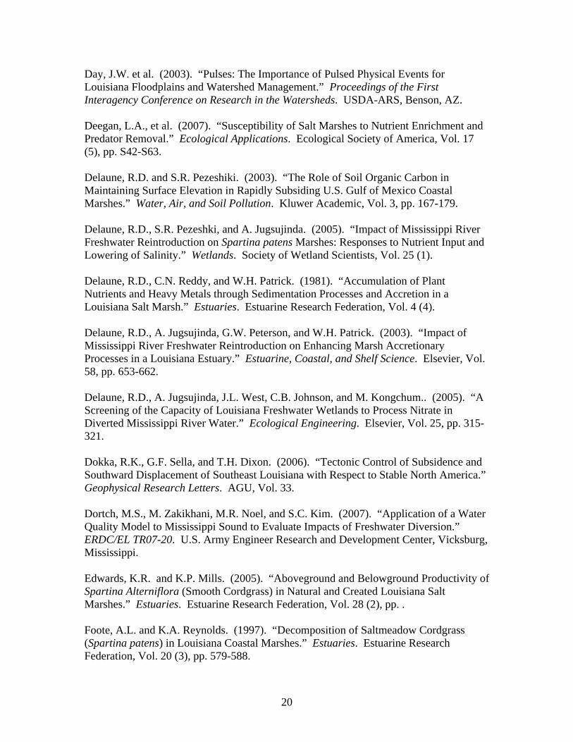
Day, J.W. et al. (2003). “Pulses: The Importance of Pulsed Physical Events for Louisiana Floodplains and Watershed Management.” Proceedings of the First Interagency Conference on Research in the Watersheds. USDA-ARS, Benson, AZ. Deegan, L.A., et al. (2007). “Susceptibility of Salt Marshes to Nutrient Enrichment and Predator Removal.” Ecological Applications. Ecological Society of America, Vol. 17 (5), pp. S42-S63. Delaune, R.D. and S.R. Pezeshiki. (2003). “The Role of Soil Organic Carbon in Maintaining Surface Elevation in Rapidly Subsiding U.S. Gulf of Mexico Coastal Marshes.” Water, Air, and Soil Pollution. Kluwer Academic, Vol. 3, pp. 167-179. Delaune, R.D., S.R. Pezeshki, and A. Jugsujinda. (2005). “Impact of Mississippi River Freshwater Reintroduction on Spartina patens Marshes: Responses to Nutrient Input and Lowering of Salinity.” Wetlands. Society of Wetland Scientists, Vol. 25 (1). Delaune, R.D., C.N. Reddy, and W.H. Patrick. (1981). “Accumulation of Plant Nutrients and Heavy Metals through Sedimentation Processes and Accretion in a Louisiana Salt Marsh.” Estuaries. Estuarine Research Federation, Vol. 4 (4). Delaune, R.D., A. Jugsujinda, G.W. Peterson, and W.H. Patrick. (2003). “Impact of Mississippi River Freshwater Reintroduction on Enhancing Marsh Accretionary Processes in a Louisiana Estuary.” Estuarine, Coastal, and Shelf Science. Elsevier, Vol. 58, pp. 653-662. Delaune, R.D., A. Jugsujinda, J.L. West, C.B. Johnson, and M. Kongchum.. (2005). “A Screening of the Capacity of Louisiana Freshwater Wetlands to Process Nitrate in Diverted Mississippi River Water.” Ecological Engineering. Elsevier, Vol. 25, pp. 315-321. Dokka, R.K., G.F. Sella, and T.H. Dixon. (2006). “Tectonic Control of Subsidence and Southward Displacement of Southeast Louisiana with Respect to Stable North America.” Geophysical Research Letters. AGU, Vol. 33. Dortch, M.S., M. Zakikhani, M.R. Noel, and S.C. Kim. (2007). “Application of a Water Quality Model to Mississippi Sound to Evaluate Impacts of Freshwater Diversion.” ERDC/EL TR07-20. U.S. Army Engineer Research and Development Center, Vicksburg, Mississippi. Edwards, K.R. and K.P. Mills. (2005). “Aboveground and Belowground Productivity of Spartina Alterniflora (Smooth Cordgrass) in Natural and Created Louisiana Salt Marshes.” Estuaries. Estuarine Research Federation, Vol. 28 (2), pp. . Foote, A.L. and K.A. Reynolds. (1997). “Decomposition of Saltmeadow Cordgrass (Spartina patens) in Louisiana Coastal Marshes.” Estuaries. Estuarine Research Federation, Vol. 20 (3), pp. 579-588.
20
Gleason, M.L., D.A. Elmer, N.C. Pien and J.S. Fisher. (1979). “Effects of Stem Density upon Sediment Retention by Salt Marsh Cordgrss, Spartina Alterniflora Loisel.” Esturaies. Estuarine Research Federation, Vol. 2 (4), pp. 271-273. Gosselink, J.G. (1984). “The Ecology of Delta Marshes of Coastal Louisiana: A Community Profile.” FWS/OBS-84109. USFWS, Washington, D.C. Hyfield, E.C.G. (2004). “Freshwater and Nutrient Inputs to a Mississippi River Deltaic Estuary with River Reintroduction.” Master’s Thesis, Louisiana State University. Hyfield, E.C.G., J.W. Day, J.E. Cable, and D. Justic. (2008). “The Impacts of Re-Introducing Mississippi River Water on the Hydrologic Budget and Nutrient Inputs of a Deltaic Estuary.” Ecological Engineering. Elsevier, Vol. 32, pp. 347-359. Kundu, P.K. (1990). Fluid Mechanics. Academic Press, San Diego. Lane, R.R., J.W. Day, and B. Thibodeaux. (1999). “Water Quality Analysis of a Freshwater Diversion at Caernarvon, Louisiana.” Estuaries. Estuarine Research Federation, Vol. 22 (2A), pp. 327-336. Leonard, L.A. and M.E. Luther. (1995). “Flow Hydrodynamics in Tidal Marsh Canopies.” Limnology and Oceanography. American Society of Limnology and Oceanography, Vol. 40 (8), pp. 1474-1484. McKay, S.K., J.C. Fischenich, and S.J. Smith. (2008). “Quantifying Benefits of Flow Diversion to Coastal Marshes. I: Theory.” In draft for submission to Ecological Engineering. Elsevier. McKay, S.K., J.C. Fischenich, and R. Paille. (2008). “Quantifying Benefits of Flow Diversion to Coastal Marshes. II: Application to Louisiana Coastal Protection and Restoration.” In draft for submission to Ecological Engineering. Elsevier. Mitsch, W.J. and B.C. Reeder. (1991). “Modelling Nutrient Retention of a Freshwater Coastal Wetland: Estimating the Roles of Primary Productivity, Sedimentation, Resuspension, and Hydrology.” Ecological Modelling. Elsevier, Vol. 54, pp. 151-187. Mitsch, W.J., J.W. Day, J.W. Gilliam, P.M. Groffman, D.L. Hey, G.W. Randall, and N. Wang. (2001). “Reducing Nitrogen Loading to the Gulf of Mexico from the Mississippi River Basin: Strategies to Counter a Persistent Ecological Problem.” Bioscience. Bioscience, Vol. 51 (5), pp. 373.388. Morris, J.T. (2007). “Ecological Engineering in Intertidal Saltmarshes.” Hydrobiologia. Springer, Vol. 577, pp. 161-168.
21

Morton, R.A., N.A. Buster, and M.D. Krohn. (2002). “Surface Controls on historical Subsidence Rates and Associated Wetland Loss in South-Central Louisiana.” Transactions of the Gulf Coast Association of Geological Societies. Vol. 52, pp. 767-778. Mossa, J. (1996). “Sediment Dynamics in the Lowermost Mississippi River.” Engineering Geology. Elsevier, Vol. 45, pp. 457-479. Nyman, J.A., R.D. Delaune, and W.H. Patrick. (1990). “Wetland Soil Formation in the Rapidly Subsiding Mississippi River Deltaic Plain: Mineral and Organic Matter Relationships.” Estuarine, Coastal, and Shelf Science. Academic Press, Vol. 31, pp.57-69. Nyman, J.A., R.D. Delaune, H.H. Roberts, and W.H. Patrick. (1993). “Relationship between Vegetation and Soil Formation in a Rapidly Submerging Coastal Marsh.” Marine Ecology Progress Series. Inter-Research, Vol. 96, pp.269-279. Nyman, J.A., R.D. Delaune, S.R. Pezeshki, and W.H. Patrick. (1995). “Organic Matter Fluxes and Marsh Stability in a Rapidly Submerging Estuarine Marsh.” Estuaries. Estuarine Research Federation, Vol. 18 (1B), pp. 207-218. Nyman, J.A., R.J. Walters, R.D. Delaune, and W.H. Patrick. (2006). “Marsh Vertical Accretion Via Vegetative Growth.” Estuarine, Coastal, and Shelf Science. Elsevier, Vol. 69, pp.370-380. Parker, G., O. Sequeiros, and River Morphodynamics Class Spring, 2006. (2006). “Large Scale River Morphodynamics: Application to the Mississippi Delta.” Proceedings River Flow 2006 Conference, Lisbon, Portugal, September 6-8, 2006, Balkema. Reed, D.J. (1995). “The Response of Coastal Marshes to Sea-Level Rise: Survival or Submergence?.” Earth Surface Processes and Landforms. John Wiley & Sons, Ltd., Vol. 20, pp. 39-48. Reyes, E., M.L. White, J.F. Martin, G.P. Kemp, J.W. Day, and V. Aravamuthan. (2000). “Landscape Modeling of Coastal Habitat Change in the Mississippi Delta.” Ecology. Ecological Society of America, Vol. 81(8), pp. 2331-2349. Reyes, E., R. Lane, and J.W. Day. (2003). “Watershed Analysis of Pulsing Freshwater Events Using Landscape Modeling in Coastal Louisiana.” Proceedings of the First Interagency Conference on Research in the Watersheds. USDA-ARS, Benson, AZ. Richardson, E.V., D.B. Simons, and P.F. Lagasse. (2001). “River Engineering for Highway Encroachments: Highways in the River Environment.” FHWA-NHI-01-004-HDS-6. FHWA, Washington, D.C.
22
Rybczyk, J.M. and D.R. Cahoon. (2002). “Estimating the Potential for Submergence for Two Wetlands in the Mississippi Delta.” Estuaries. Estuarine Research Federation, Vol. 25 (5), pp. 985-998. Snedden, G.A., J.E. Cable, C. Swarzenski, and E. Swenson. (2007). “Sediment Discharge into a Subsiding Louisiana Deltaic Estuary Through a Mississippi River Diversion.” Estuarine, Coastal, and Shelf Science. Elsevier, Vol. 71, pp.181-193. Soulsby, R.L. (1983). “The bottom boundary layer of shelf seas.” In Physical Oceanography of Coastal and Shelf Seas, ed. B. Johns, pp. 189-266. Elsevier, Amsterdam. Soulsby, R.L. (1997). “Dynamics of marine sands.” Thomas Telford, London. Stumpf, R.P. (1983). “The Process of Sedimentation on the Surface of a Salt Marsh.” Estuarine, Coastal, and Shelf Science. Academic Press Inc., Vol. 17, pp. 495-508. United States Army Corps of Engineers (USACE). (2006). “Louisiana Coastal Protection and Restoration: A Preliminary Technical Report to United States Congress.” U.S. Army Corps of Engineers, New Orleans District, New Orleans, Louisiana. Visser, J.M. et al. (2004). “Chapter C.9: Habitat Switching Module.” In Louisiana Coastal Area (LCA) Ecosystem Restoration Study, Appendix C. U.S. Army Corps of Engineers, New Orleans, Louisiana. Wang, F.C. (1997). “Dynamics of Intertidal Marshes near Shallow Estuaries in Louisiana.” Wetlands Ecology and Management. Kluwer Academic, Vol. 5, pp.131-143. White, F. M. (2003). Fluid Mechanics: Fifth Edition. McGraw-Hill, New York, New York. Winterwep, J.C. and W.G.M. van Kesteren. (2004). Introduction to the Physics of Cohesive Sediment in the Marine Environment. Developments in Sedimentology Series No. 56 xiii, 446 pp. Elsevier, Amsterdam, The Netherlands.
23

Figures
Figure 1. Typical coastal Louisiana marsh community with a patchwork of dense vegetation and open water
24
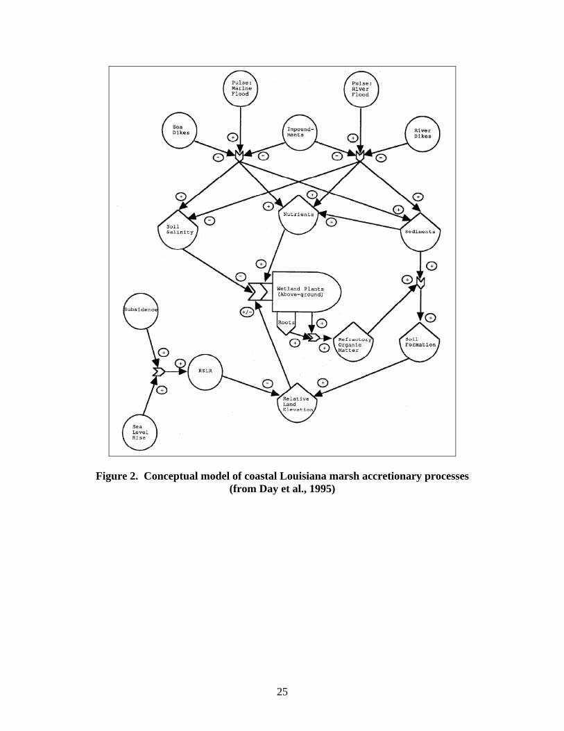
Figure 2. Conceptual model of coastal Louisiana marsh accretionary processes (from Day et al., 1995)
25
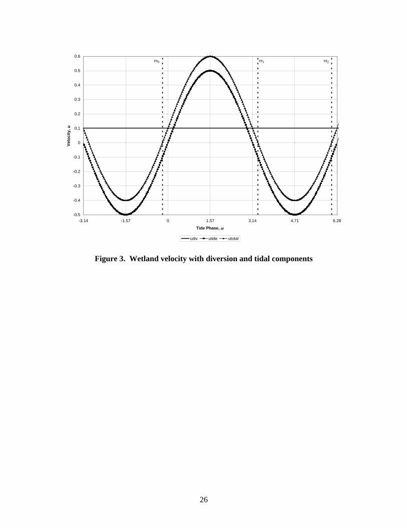
-0.5
-0.4
-0.3
-0.2
-0.1
0
0.1
0.2
0.3
0.4
0.5
0.6
-3.14 -1.57 0 1.57 3.14 4.71 6.28
Tide Phase, ω
Velo
city
, u
udiv utide utotal
ω0 ω1 ω2
Figure 3. Wetland velocity with diversion and tidal components
26

Figure 4. Aerial view of Breton Sound displaying Caernarvon Diversion and project division areas for tracking land evolution. In this analysis only the following
areas were considered to be directly influenced by the Caernarvon Diversion in order to maintain relative uniformity in conditions: Upper Reference Outfall East, Upper Project Outfall, Upper Reference West, Middle Reference West, and Middle
Project Area.
27
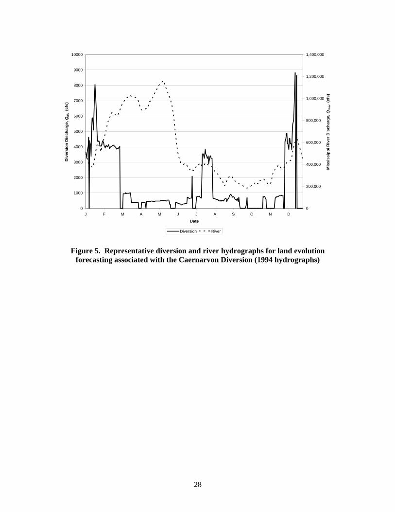
0
1000
2000
3000
4000
5000
6000
7000
8000
9000
10000
J F M A M J J A S O N D
Date
Div
ersi
on D
isch
arge
, Qdi
v (c
fs)
0
200,000
400,000
600,000
800,000
1,000,000
1,200,000
1,400,000
Mis
siss
ippi
Riv
er D
isch
arge
, Qriv
er (c
fs)
Diversion River
Figure 5. Representative diversion and river hydrographs for land evolution forecasting associated with the Caernarvon Diversion (1994 hydrographs)
28
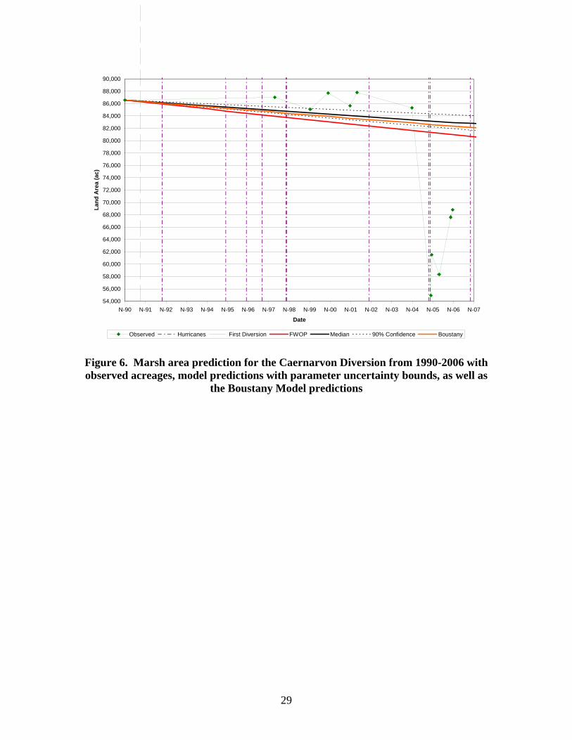
54,000
56,000
58,000
60,000
62,000
64,000
66,000
68,000
70,000
72,000
74,000
76,000
78,000
80,000
82,000
84,000
86,000
88,000
90,000
N-90 N-91 N-92 N-93 N-94 N-95 N-96 N-97 N-98 N-99 N-00 N-01 N-02 N-03 N-04 N-05 N-06 N-07
Date
Land
Are
a (a
c)
Observed Hurricanes First Diversion FWOP Median 90% Confidence Boustany
Figure 6. Marsh area prediction for the Caernarvon Diversion from 1990-2006 with observed acreages, model predictions with parameter uncertainty bounds, as well as
the Boustany Model predictions
29
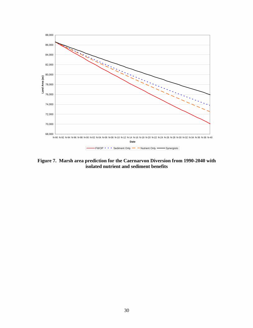
68,000
70,000
72,000
74,000
76,000
78,000
80,000
82,000
84,000
86,000
88,000
N-90 N-92 N-94 N-96 N-98 N-00 N-02 N-04 N-06 N-08 N-10 N-12 N-14 N-16 N-18 N-20 N-22 N-24 N-26 N-28 N-30 N-32 N-34 N-36 N-38 N-40
Date
Land
Are
a (a
c)
FWOP Sediment Only Nutrient Only Synergistic
Figure 7. Marsh area prediction for the Caernarvon Diversion from 1990-2040 with isolated nutrient and sediment benefits
30
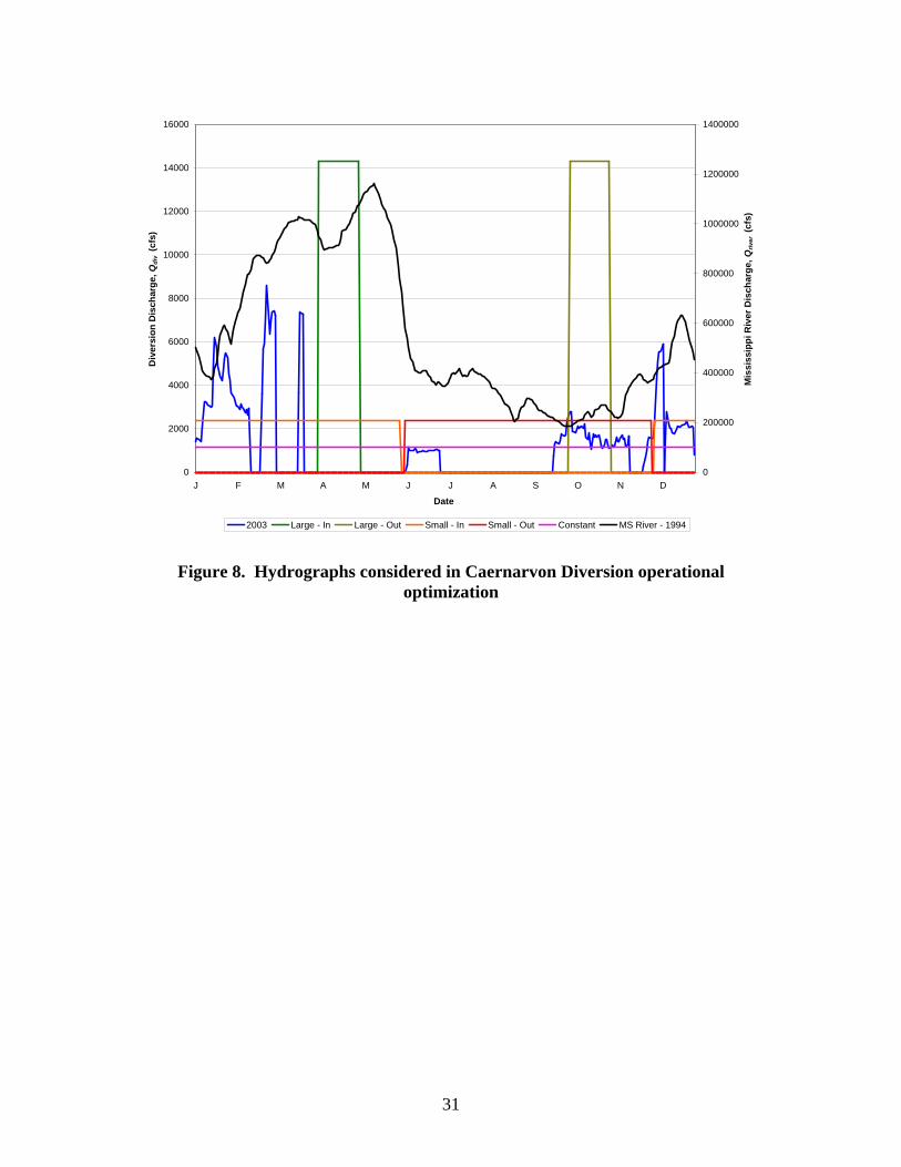
0
2000
4000
6000
8000
10000
12000
14000
16000
J F M A M J J A S O N D
Date
Div
ersi
on D
isch
arge
, Qdi
v (c
fs)
0
200000
400000
600000
800000
1000000
1200000
1400000
Mis
siss
ippi
Riv
er D
isch
arge
, Qriv
er (c
fs)
2003 Large - In Large - Out Small - In Small - Out Constant MS River - 1994
Figure 8. Hydrographs considered in Caernarvon Diversion operational
optimization
31
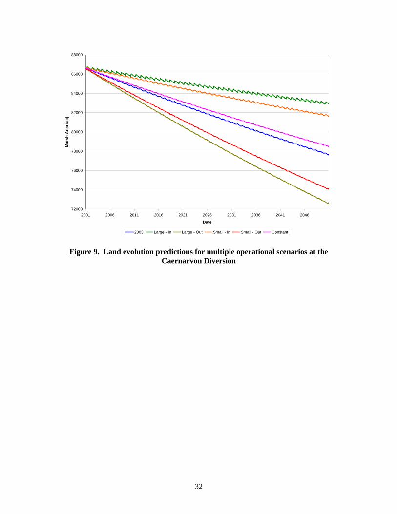
72000
74000
76000
78000
80000
82000
84000
86000
88000
2001 2006 2011 2016 2021 2026 2031 2036 2041 2046
Date
Mar
sh A
rea
(ac)
2003 Large - In Large - Out Small - In Small - Out Constant
Figure 9. Land evolution predictions for multiple operational scenarios at the Caernarvon Diversion
32
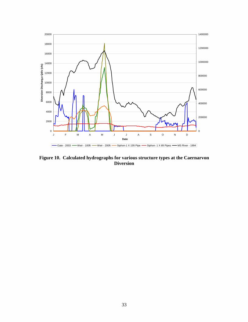
0
2000
4000
6000
8000
10000
12000
14000
16000
18000
20000
J F M A M J J A S O N D
Date
Div
ersi
on D
isch
arg,
e Q
div
(cfs
)
0
200000
400000
600000
800000
1000000
1200000
1400000
Gate - 2003 Weir - 100ft Weir - 200ft Siphon-1 X 15ft Pipe Siphon- 1 X 6ft Pipes MS River - 1994
Figure 10. Calculated hydrographs for various structure types at the Caernarvon Diversion
33
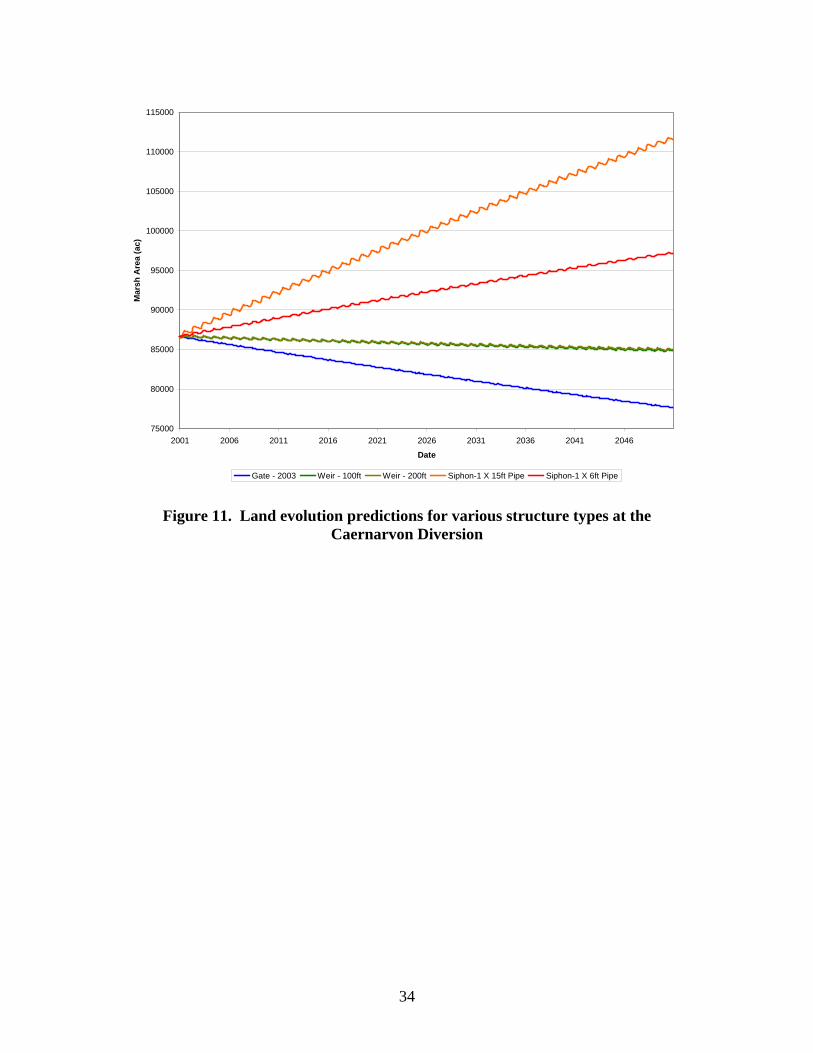
75000
80000
85000
90000
95000
100000
105000
110000
115000
2001 2006 2011 2016 2021 2026 2031 2036 2041 2046
Date
Mar
sh A
rea
(ac)
Gate - 2003 Weir - 100ft Weir - 200ft Siphon-1 X 15ft Pipe Siphon-1 X 6ft Pipe
Figure 11. Land evolution predictions for various structure types at the Caernarvon Diversion
34
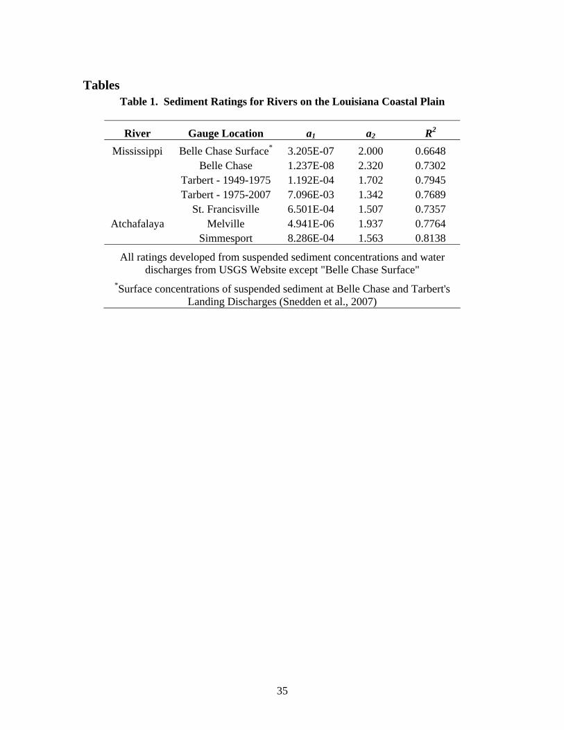
Tables Table 1. Sediment Ratings for Rivers on the Louisiana Coastal Plain
River Gauge Location a1 a2 R2
Mississippi Belle Chase Surface* 3.205E-07 2.000 0.6648 Belle Chase 1.237E-08 2.320 0.7302 Tarbert - 1949-1975 1.192E-04 1.702 0.7945 Tarbert - 1975-2007 7.096E-03 1.342 0.7689 St. Francisville 6.501E-04 1.507 0.7357 Atchafalaya Melville 4.941E-06 1.937 0.7764 Simmesport 8.286E-04 1.563 0.8138
All ratings developed from suspended sediment concentrations and water discharges from USGS Website except "Belle Chase Surface"
*Surface concentrations of suspended sediment at Belle Chase and Tarbert's Landing Discharges (Snedden et al., 2007)
35
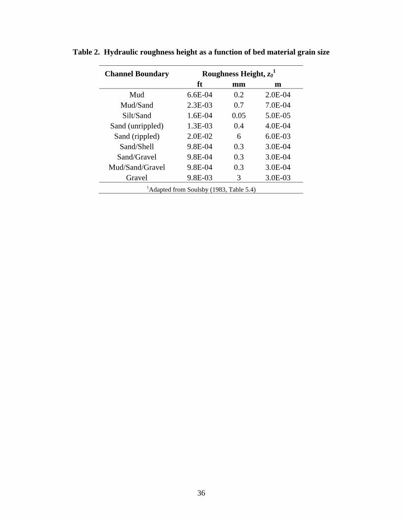
36
Table 2. Hydraulic roughness height as a function of bed material grain size
Channel Boundary Roughness Height, z01
ft mm m Mud 6.6E-04 0.2 2.0E-04
Mud/Sand 2.3E-03 0.7 7.0E-04 Silt/Sand 1.6E-04 0.05 5.0E-05
Sand (unrippled) 1.3E-03 0.4 4.0E-04 Sand (rippled) 2.0E-02 6 6.0E-03
Sand/Shell 9.8E-04 0.3 3.0E-04 Sand/Gravel 9.8E-04 0.3 3.0E-04
Mud/Sand/Gravel 9.8E-04 0.3 3.0E-04 Gravel 9.8E-03 3 3.0E-03
1Adapted from Soulsby (1983, Table 5.4)
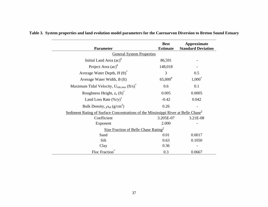
Table 3. System properties and land evolution model parameters for the Caernarvon Diversion to Breton Sound Estuary
Parameter Best
Estimate Approximate
Standard Deviation General System Properties
Initial Land Area (ac)# 86,591 - Project Area (ac)# 148,018 -
Average Water Depth, H (ft)* 3 0.5 Average Water Width, B (ft) 65,000# 1,000*
Maximum Tidal Velocity, Utide,max (ft/s)* 0.6 0.1
Roughness Height, zo (ft)* 0.005 0.0005 Land Loss Rate (%/y)1 -0.42 0.042
Bulk Density, ρbd (g/cm3) 0.26 - Sediment Rating of Surface Concentrations of the Mississippi River at Belle Chase2
Coefficient 3.205E-07 3.21E-08 Exponent 2.000 -
Size Fraction of Belle Chase Rating2
Sand 0.01 0.0017 Silt 0.63 0.1050
Clay 0.36 - Floc Fraction* 0.3 0.0667
37

38
Parameter Best
Estimate Approximate
Standard Deviation Approximate Fall Velocity3 (m/s)
Sand 1.00E-02 8.33E-04 Silt 3.00E-04 2.50E-05 Clay 7.00E-06 5.83E-07
Floc Fraction 2.00E-04 4.00E-05 Marsh Nutrient Requirements
Plant Productivity Rate, Pr (g/m2yr)* 4,150 415
Percent of N and P in Plant Biomass, γTNP(%)4 0.72 0.072*
Nutrient Loading to Marsh
Background Concentration of N and P, Cbackground (mg/L)5 0.34 0.034*
Sourcewater Concentration of N and P, Csource (mg/L)# 2.28 0.5*
Nutrient Retention, Rnut (%)* 50 10 1Land loss rate calculated from observed marsh acreage from 1978-1990
2Data for rating and size fraction from Snedden et al. (2007) 3Calculated from method of Soulsby (1997)
4Foote and Reynolds (1997) 5Hyfield (2004) #Available data
*Best professional judgment
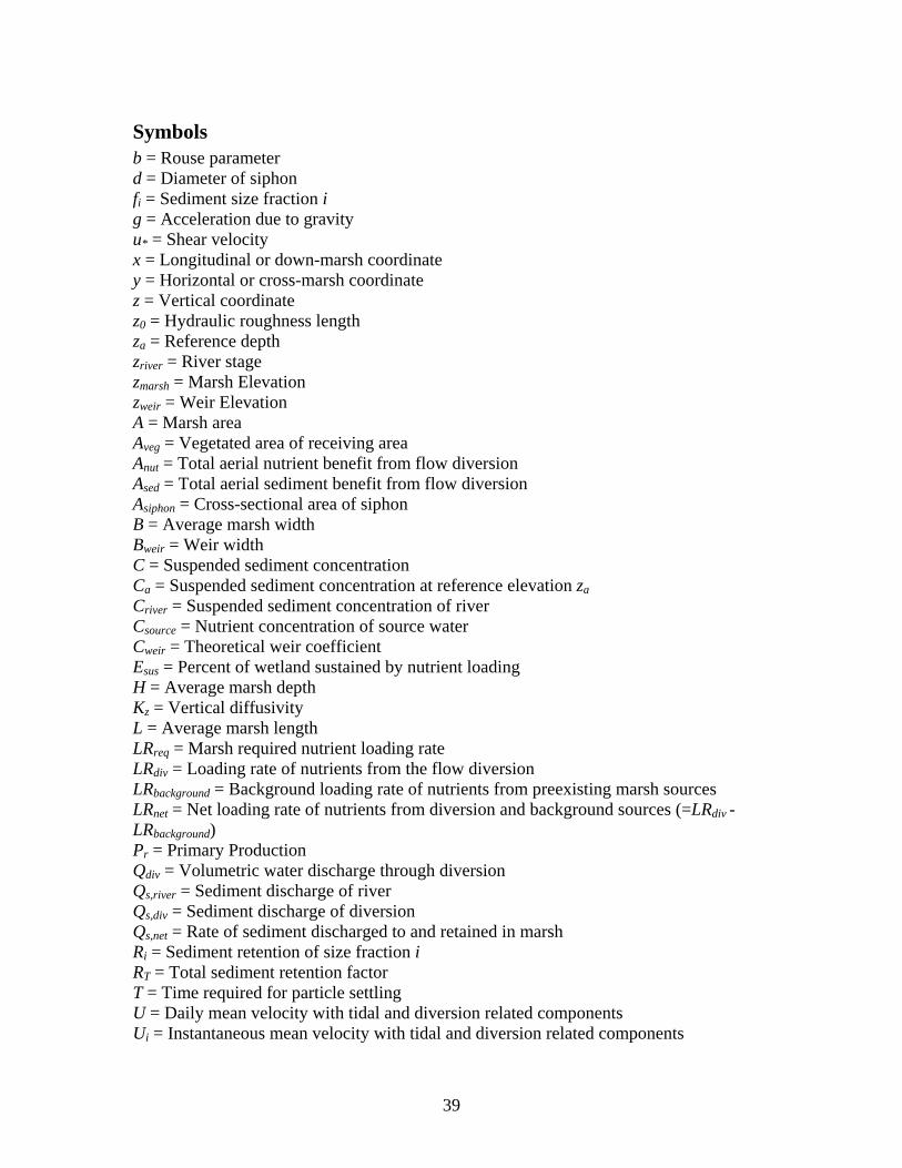
Symbols b = Rouse parameter d = Diameter of siphon fi = Sediment size fraction i g = Acceleration due to gravity u* = Shear velocity x = Longitudinal or down-marsh coordinate y = Horizontal or cross-marsh coordinate z = Vertical coordinate z0 = Hydraulic roughness length za = Reference depth zriver = River stage zmarsh = Marsh Elevation zweir = Weir Elevation A = Marsh area Aveg = Vegetated area of receiving area Anut = Total aerial nutrient benefit from flow diversion Ased = Total aerial sediment benefit from flow diversion Asiphon = Cross-sectional area of siphon B = Average marsh width BBweir = Weir width C = Suspended sediment concentration Ca = Suspended sediment concentration at reference elevation zaCriver = Suspended sediment concentration of river Csource = Nutrient concentration of source water Cweir = Theoretical weir coefficient Esus = Percent of wetland sustained by nutrient loading H = Average marsh depth Kz = Vertical diffusivity L = Average marsh length LRreq = Marsh required nutrient loading rate LRdiv = Loading rate of nutrients from the flow diversion LRbackground = Background loading rate of nutrients from preexisting marsh sources LRnet = Net loading rate of nutrients from diversion and background sources (=LRdiv - LRbackground) Pr = Primary Production Qdiv = Volumetric water discharge through diversion Qs,river = Sediment discharge of river Qs,div = Sediment discharge of diversion Qs,net = Rate of sediment discharged to and retained in marsh Ri = Sediment retention of size fraction i RT = Total sediment retention factor T = Time required for particle settling U = Daily mean velocity with tidal and diversion related components Ui = Instantaneous mean velocity with tidal and diversion related components
39

Udiv = Diversion induced velocity (= Qdiv / HB) Umax,tide = Maximum tidal velocity (tidal velocity amplitude) Vsiphon = Velocity of flow in siphon Ws = Natural settling velocity Ws,eff = Effective settling velocity due to natural settling and turbulence X = Transport distance of suspended sediment δ = Land change rate (% / time) δnut = Nutrient suppressed land change rate (% / time) γnut = Percent of plant biomass made up of nutrients κ = von Karman’s constant (0.4) ω = Tide phase ω0 = Tide phase of the up-crossing zero velocity ω1 = Tide phase of the down-crossing zero velocity (=ω0 + π) ω2 = ω0 + 2π
40

Volume III – Convey Atchafalaya River Water to Northern Terrebonne Marshes and Multipurpose Operation of Houma Navigation Lock – Appendix M – Wetland Value Assessment (WVA)
Annex 4. SAND2 and WVA Data Summary Tables.
Table 1. SAND2 Model Determined Wetland Acreages Associated with Study Area Polygons Receiving Diversion Benefits (or Impacts).
Palmetto Bayou, Creole Bayou
A6, A&, Lake Pagie
C9 C2-C7 Bayou Dulac E2-E4 G2, G3, G6 F2 G1, G5 B6, B7 C11-C14 TOTAL
Net
FWOP FWP FWOP FWP FWOP FWP FWOP FWP FWOP FWP FWOP FWP FWOP FWP FWOP FWP FWOP FWP FWOP FWP FWOP FWP FWOP FWP TY50
TY Year (acres) (acres) (acres) (acres) (acres) (acres) (acres) (acres) (acres) (acres) (acres) (acres) (acres) (acres) (acres) (acres) (acres) (acres) (acres) (acres) (acres) (acres) (acres) (acres) (acres)
0 2015 50,083 50,083 16,569 16,569 960 960 13,003 13,003 2,393 2,393 7,133 7,133 17,466 17,466 1,428 1,428 20,401 20,401 23,931 23,931 19,924 19,924 346,581 346,581
Alt 2 1 2016 50,046 50,046 16,337 16,451 947 957 12,757 12,728 2,368 2,408 6,590 6,563 17,156 17,243 1,357 1,342 20,327 20,074 23,742 23,742 19,715 19,734 171,340 171,287
10 2025 49,710 49,710 14,245 15,443 827 933 10,543 10,683 2,143 2,176 1,696 1,669 14,365 15,244 717 574 19,662 19,409 22,042 22,110 17,837 17,844 153,786 155,794
50 2065 48,217 48,217 6,343 14,230 286 882 2,925 3,766 1,145 885 0 0 5,188 10,010 0 0 16,930 16,677 14,486 17,276 9,488 2,961 105,007 114,902 9,895
Alt 3 1 2016 50,046 50,046 16,337 16,455 947 957 12,757 12,728 2,368 2,408 6,590 6,563 17,156 17,244 1,357 1,342 20,327 20,074 23,742 23,742 19,715 19,735 171,340 171,293
10 2025 49,710 49,710 14,245 15,475 827 935 10,543 10,686 2,143 2,176 1,696 1,669 14,365 15,254 717 574 19,662 19,409 22,042 22,111 17,837 17,849 153,786 155,847
50 2065 48,217 48,217 6,343 14,361 286 889 2,925 3,779 1,145 893 0 0 5,188 10,068 0 0 16,930 16,677 14,486 17,319 9,488 2,979 105,007 115,181 10,174
Alt 4 1 2016 50,046 50,046 16,337 16,451 947 957 12,757 12,726 2,368 2,408 6,590 6,563 17,156 17,310 1,357 1,343 20,327 20,074 23,742 23,742 19,715 19,732 171,340 171,351
10 2025 49,710 49,710 14,245 15,435 827 926 10,543 10,666 2,143 2,176 1,696 1,669 14,365 15,908 717 586 19,662 19,409 22,042 22,109 17,837 17,823 153,786 156,416
50 2065 48,217 48,217 6,343 14,126 286 846 2,925 3,682 1,145 879 0 0 5,188 12,886 0 0 16,930 16,677 14,486 17,253 9,488 2,938 105,007 117,503 12,495
Alt 5 1 2016 50,046 50,046 16,337 16,452 947 957 12,757 12,726 2,368 2,390 6,590 6,563 17,156 17,310 1,357 1,343 20,327 20,074 23,742 23,742 19,715 19,733 171,340 171,336
10 2025 49,710 49,710 14,245 15,452 827 927 10,543 10,668 2,143 2,397 1,696 1,669 14,365 15,908 717 586 19,662 19,409 22,042 22,110 17,837 17,833 153,786 156,670
50 2065 48,217 48,217 6,343 14,275 286 853 2,925 3,690 1,145 1,994 0 0 5,188 12,887 0 0 16,930 16,677 14,486 17,302 9,488 2,963 105,007 118,858 13,850
Alt 6 1 2016 50,046 50,046 16,337 16,337 947 947 12,757 12,707 2,368 2,379 6,590 6,590 17,156 17,196 1,357 1,358 20,327 20,327 23,742 23,742 19,715 19,715 171,340 171,344
10 2025 49,710 49,710 14,245 14,265 827 827 10,543 10,480 2,143 2,279 1,696 1,696 14,365 14,768 717 739 19,662 19,662 22,042 22,095 17,837 17,668 153,786 154,188
50 2065 48,217 48,217 6,343 7,205 286 286 2,925 2,862 1,145 2,578 0 0 5,188 7,364 0 0 16,930 16,930 14,486 16,678 9,488 2,535 105,007 104,654 -354
Alt 7 1 2016 50,046 50,046 16,337 16,337 947 947 12,757 12,709 2,368 2,368 6,590 6,590 17,156 17,156 1,357 1,357 20,327 20,327 23,742 23,742 19,715 19,715 171,340 171,292
10 2025 49,710 49,710 14,245 14,265 827 827 10,543 10,495 2,143 2,175 1,696 1,696 14,365 14,365 717 717 19,662 19,662 22,042 22,095 17,837 17,668 153,786 153,675
50 2065 48,217 48,217 6,343 7,194 286 286 2,925 2,877 1,145 2,458 0 0 5,188 5,188 0 0 16,930 16,930 14,486 16,676 9,488 2,532 105,007 102,357 -2,651
Alt 8 1 2016 50,046 50,046 16,337 16,335 947 956 12,757 12,728 2,368 2,368 6,590 6,590 17,156 16,972 1,357 1,342 20,327 20,327 23,742 23,742 19,715 19,715 171,340 171,120
10 2025 49,710 49,710 14,245 14,243 827 917 10,543 10,685 2,143 2,133 1,696 1,696 14,365 14,888 717 573 19,662 19,662 22,042 22,099 17,837 17,673 153,786 154,279
50 2065 48,217 48,217 6,343 7,011 286 684 2,925 3,772 1,145 727 0 0 5,188 9,151 0 0 16,930 16,930 14,486 16,822 9,488 2,707 105,007 106,021 1,013
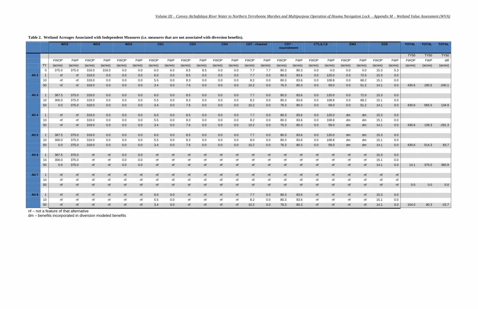
Volume III – Convey Atchafalaya River Water to Northern Terrebonne Marshes and Multipurpose Operation of Houma Navigation Lock – Appendix M – Wetland Value Assessment (WVA)
Table 2. Wetland Acreages Associated with Independent Measures (i.e. measures that are not associated with diversion benefits).
nf – not a feature of that alternative dm – benefits incorporated in diversion modeled benefits
WO2 WD2 WD3 CD1 CD3 CD4 CD7 - channel CD7 - nourishment
CT1,6,7,8 EM3 ED5 TOTAL TOTAL TOTAL
TY50 TY50 TY50
FWOP FWP FWOP FWP FWOP FWP FWOP FWP FWOP FWP FWOP FWP FWOP FWP FWOP FWP FWOP FWP FWOP FWP FWOP FWP FWOP FWP diff
TY (acres) (acres) (acres) (acres) (acres) (acres) (acres) (acres) (acres) (acres) (acres) (acres) (acres) (acres) (acres) (acres) (acres) (acres) (acres) (acres) (acres) (acres) (acres) (acres) (acres)
0 375.0 375.0 319.0 319.0 0.0 0.0 6.0 6.0 8.5 8.5 0.0 0.0 7.7 7.7 80.3 80.3 0.0 0.0 0.0 0.0 15.3 5.3
Alt 2 1 nf nf 319.0 0.0 0.0 0.0 6.0 0.0 8.5 0.0 0.0 0.0 7.7 0.0 80.3 83.6 0.0 120.0 0.0 72.0 15.3 0.0
10 nf nf 319.0 0.0 0.0 0.0 5.5 0.0 8.3 0.0 0.0 0.0 8.2 0.0 80.3 83.6 0.0 108.8 0.0 68.2 15.1 0.0
50 nf nf 319.0 0.0 0.0 0.0 3.4 0.0 7.6 0.0 0.0 0.0 10.2 0.0 76.3 80.3 0.0 59.0 0.0 51.2 14.1 0.0 430.6 190.5 -240.1
Alt 3 1 367.5 375.0 319.0 0.0 0.0 0.0 6.0 0.0 8.5 0.0 0.0 0.0 7.7 0.0 80.3 83.6 0.0 120.0 0.0 72.0 15.3 0.0
10 300.0 375.0 319.0 0.0 0.0 0.0 5.5 0.0 8.3 0.0 0.0 0.0 8.2 0.0 80.3 83.6 0.0 108.8 0.0 68.2 15.1 0.0
50 0.0 375.0 319.0 0.0 0.0 0.0 3.4 0.0 7.6 0.0 0.0 0.0 10.2 0.0 76.3 80.3 0.0 59.0 0.0 51.2 14.1 0.0 430.6 565.5 134.9
Alt 4 1 nf nf 319.0 0.0 0.0 0.0 6.0 0.0 8.5 0.0 0.0 0.0 7.7 0.0 80.3 83.6 0.0 120.0 dm dm 15.3 0.0
10 nf nf 319.0 0.0 0.0 0.0 5.5 0.0 8.3 0.0 0.0 0.0 8.2 0.0 80.3 83.6 0.0 108.8 dm dm 15.1 0.0
50 nf nf 319.0 0.0 0.0 0.0 3.4 0.0 7.6 0.0 0.0 0.0 10.2 0.0 76.3 80.3 0.0 59.0 dm dm 14.1 0.0 430.6 139.3 -291.3
Alt 5 1 367.5 375.0 319.0 0.0 0.0 0.0 6.0 0.0 8.5 0.0 0.0 0.0 7.7 0.0 80.3 83.6 0.0 120.0 dm dm 15.3 0.0
10 300.0 375.0 319.0 0.0 0.0 0.0 5.5 0.0 8.3 0.0 0.0 0.0 8.0 0.0 80.3 83.6 0.0 108.8 dm dm 15.1 0.0
50 0.0 375.0 319.0 0.0 0.0 0.0 3.4 0.0 7.6 0.0 0.0 0.0 10.2 0.0 76.3 80.3 0.0 59.0 dm dm 14.1 0.0 430.6 514.3 83.7
Alt 6 1 367.5 375.0 nf nf 0.0 0.0 nf nf nf nf nf nf nf nf nf nf nf nf nf nf 15.3 0.0
10 300.0 375.0 nf nf 0.0 0.0 nf nf nf nf nf nf nf nf nf nf nf nf nf nf 15.1 0.0
50 0.0 375.0 nf nf 0.0 0.0 nf nf nf nf nf nf nf nf nf nf nf nf nf nf 14.1 0.0 14.1 375.0 360.9
Alt 7 1 nf nf nf nf nf nf nf nf nf nf nf nf nf nf nf nf nf nf nf nf nf nf
10 nf nf nf nf nf nf nf nf nf nf nf nf nf nf nf nf nf nf nf nf nf nf
50 nf nf nf nf nf nf nf nf nf nf nf nf nf nf nf nf nf nf nf nf nf nf 0.0 0.0 0.0
Alt 8 1 nf nf nf nf nf nf 6.0 0.0 nf nf nf nf 7.7 0.0 80.3 83.6 nf nf nf nf 15.3 0.0
10 nf nf nf nf nf nf 5.5 0.0 nf nf nf nf 8.2 0.0 80.3 83.6 nf nf nf nf 15.1 0.0
50 nf nf nf nf nf nf 3.4 0.0 nf nf nf nf 10.2 0.0 76.3 80.3 nf nf nf nf 14.1 0.0 104.0 80.3 -23.7
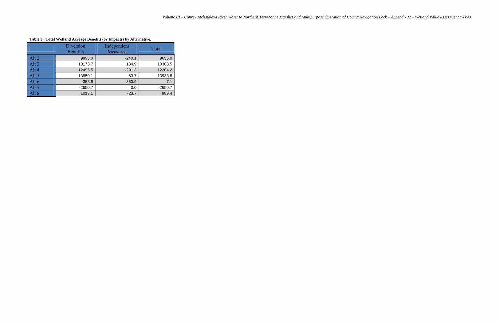
Volume III – Convey Atchafalaya River Water to Northern Terrebonne Marshes and Multipurpose Operation of Houma Navigation Lock – Appendix M – Wetland Value Assessment (WVA)
Table 3. Total Wetland Acreage Benefits (or Impacts) by Alternative.
Diversion Benefits
Independent Measures Total
Alt 2 9895.0 -240.1 9655.0
Alt 3 10173.7 134.9 10308.5
Alt 4 12495.5 -291.3 12204.2
Alt 5 13850.1 83.7 13933.8
Alt 6 -353.8 360.9 7.1
Alt 7 -2650.7 0.0 -2650.7
Alt 8 1013.1 -23.7 989.4
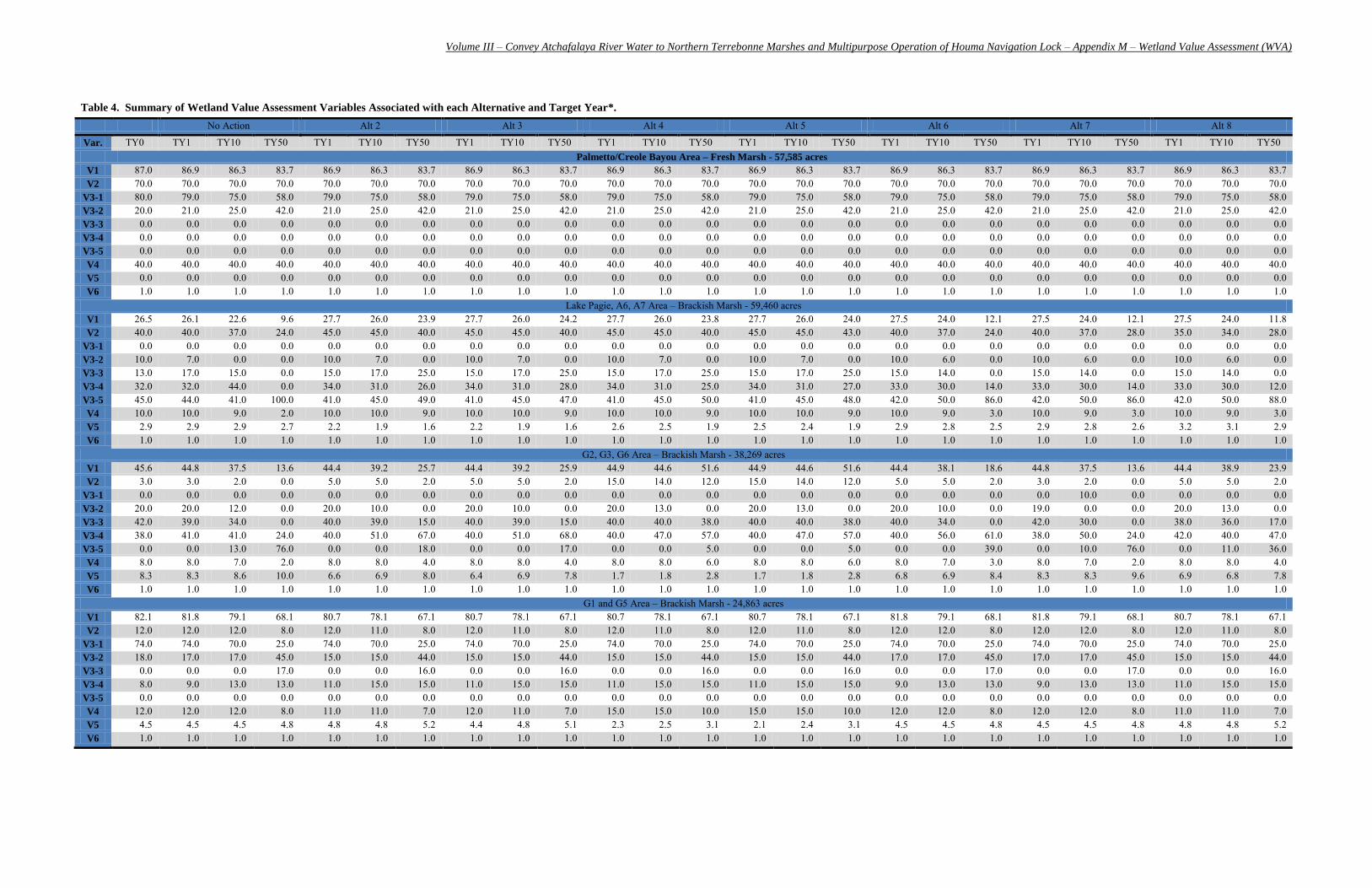
Volume III – Convey Atchafalaya River Water to Northern Terrebonne Marshes and Multipurpose Operation of Houma Navigation Lock – Appendix M – Wetland Value Assessment (WVA)
Table 4. Summary of Wetland Value Assessment Variables Associated with each Alternative and Target Year*.
No Action Alt 2 Alt 3 Alt 4 Alt 5 Alt 6 Alt 7 Alt 8
Var. TY0 TY1 TY10 TY50 TY1 TY10 TY50 TY1 TY10 TY50 TY1 TY10 TY50 TY1 TY10 TY50 TY1 TY10 TY50 TY1 TY10 TY50 TY1 TY10 TY50 Palmetto/Creole Bayou Area – Fresh Marsh - 57,585 acres
V1 87.0 86.9 86.3 83.7 86.9 86.3 83.7 86.9 86.3 83.7 86.9 86.3 83.7 86.9 86.3 83.7 86.9 86.3 83.7 86.9 86.3 83.7 86.9 86.3 83.7 V2 70.0 70.0 70.0 70.0 70.0 70.0 70.0 70.0 70.0 70.0 70.0 70.0 70.0 70.0 70.0 70.0 70.0 70.0 70.0 70.0 70.0 70.0 70.0 70.0 70.0
V3-1 80.0 79.0 75.0 58.0 79.0 75.0 58.0 79.0 75.0 58.0 79.0 75.0 58.0 79.0 75.0 58.0 79.0 75.0 58.0 79.0 75.0 58.0 79.0 75.0 58.0 V3-2 20.0 21.0 25.0 42.0 21.0 25.0 42.0 21.0 25.0 42.0 21.0 25.0 42.0 21.0 25.0 42.0 21.0 25.0 42.0 21.0 25.0 42.0 21.0 25.0 42.0 V3-3 0.0 0.0 0.0 0.0 0.0 0.0 0.0 0.0 0.0 0.0 0.0 0.0 0.0 0.0 0.0 0.0 0.0 0.0 0.0 0.0 0.0 0.0 0.0 0.0 0.0 V3-4 0.0 0.0 0.0 0.0 0.0 0.0 0.0 0.0 0.0 0.0 0.0 0.0 0.0 0.0 0.0 0.0 0.0 0.0 0.0 0.0 0.0 0.0 0.0 0.0 0.0 V3-5 0.0 0.0 0.0 0.0 0.0 0.0 0.0 0.0 0.0 0.0 0.0 0.0 0.0 0.0 0.0 0.0 0.0 0.0 0.0 0.0 0.0 0.0 0.0 0.0 0.0 V4 40.0 40.0 40.0 40.0 40.0 40.0 40.0 40.0 40.0 40.0 40.0 40.0 40.0 40.0 40.0 40.0 40.0 40.0 40.0 40.0 40.0 40.0 40.0 40.0 40.0 V5 0.0 0.0 0.0 0.0 0.0 0.0 0.0 0.0 0.0 0.0 0.0 0.0 0.0 0.0 0.0 0.0 0.0 0.0 0.0 0.0 0.0 0.0 0.0 0.0 0.0 V6 1.0 1.0 1.0 1.0 1.0 1.0 1.0 1.0 1.0 1.0 1.0 1.0 1.0 1.0 1.0 1.0 1.0 1.0 1.0 1.0 1.0 1.0 1.0 1.0 1.0
Lake Pagie, A6, A7 Area – Brackish Marsh - 59,460 acres V1 26.5 26.1 22.6 9.6 27.7 26.0 23.9 27.7 26.0 24.2 27.7 26.0 23.8 27.7 26.0 24.0 27.5 24.0 12.1 27.5 24.0 12.1 27.5 24.0 11.8 V2 40.0 40.0 37.0 24.0 45.0 45.0 40.0 45.0 45.0 40.0 45.0 45.0 40.0 45.0 45.0 43.0 40.0 37.0 24.0 40.0 37.0 28.0 35.0 34.0 28.0
V3-1 0.0 0.0 0.0 0.0 0.0 0.0 0.0 0.0 0.0 0.0 0.0 0.0 0.0 0.0 0.0 0.0 0.0 0.0 0.0 0.0 0.0 0.0 0.0 0.0 0.0 V3-2 10.0 7.0 0.0 0.0 10.0 7.0 0.0 10.0 7.0 0.0 10.0 7.0 0.0 10.0 7.0 0.0 10.0 6.0 0.0 10.0 6.0 0.0 10.0 6.0 0.0 V3-3 13.0 17.0 15.0 0.0 15.0 17.0 25.0 15.0 17.0 25.0 15.0 17.0 25.0 15.0 17.0 25.0 15.0 14.0 0.0 15.0 14.0 0.0 15.0 14.0 0.0 V3-4 32.0 32.0 44.0 0.0 34.0 31.0 26.0 34.0 31.0 28.0 34.0 31.0 25.0 34.0 31.0 27.0 33.0 30.0 14.0 33.0 30.0 14.0 33.0 30.0 12.0 V3-5 45.0 44.0 41.0 100.0 41.0 45.0 49.0 41.0 45.0 47.0 41.0 45.0 50.0 41.0 45.0 48.0 42.0 50.0 86.0 42.0 50.0 86.0 42.0 50.0 88.0 V4 10.0 10.0 9.0 2.0 10.0 10.0 9.0 10.0 10.0 9.0 10.0 10.0 9.0 10.0 10.0 9.0 10.0 9.0 3.0 10.0 9.0 3.0 10.0 9.0 3.0 V5 2.9 2.9 2.9 2.7 2.2 1.9 1.6 2.2 1.9 1.6 2.6 2.5 1.9 2.5 2.4 1.9 2.9 2.8 2.5 2.9 2.8 2.6 3.2 3.1 2.9 V6 1.0 1.0 1.0 1.0 1.0 1.0 1.0 1.0 1.0 1.0 1.0 1.0 1.0 1.0 1.0 1.0 1.0 1.0 1.0 1.0 1.0 1.0 1.0 1.0 1.0
G2, G3, G6 Area – Brackish Marsh - 38,269 acres V1 45.6 44.8 37.5 13.6 44.4 39.2 25.7 44.4 39.2 25.9 44.9 44.6 51.6 44.9 44.6 51.6 44.4 38.1 18.6 44.8 37.5 13.6 44.4 38.9 23.9 V2 3.0 3.0 2.0 0.0 5.0 5.0 2.0 5.0 5.0 2.0 15.0 14.0 12.0 15.0 14.0 12.0 5.0 5.0 2.0 3.0 2.0 0.0 5.0 5.0 2.0
V3-1 0.0 0.0 0.0 0.0 0.0 0.0 0.0 0.0 0.0 0.0 0.0 0.0 0.0 0.0 0.0 0.0 0.0 0.0 0.0 0.0 10.0 0.0 0.0 0.0 0.0 V3-2 20.0 20.0 12.0 0.0 20.0 10.0 0.0 20.0 10.0 0.0 20.0 13.0 0.0 20.0 13.0 0.0 20.0 10.0 0.0 19.0 0.0 0.0 20.0 13.0 0.0 V3-3 42.0 39.0 34.0 0.0 40.0 39.0 15.0 40.0 39.0 15.0 40.0 40.0 38.0 40.0 40.0 38.0 40.0 34.0 0.0 42.0 30.0 0.0 38.0 36.0 17.0 V3-4 38.0 41.0 41.0 24.0 40.0 51.0 67.0 40.0 51.0 68.0 40.0 47.0 57.0 40.0 47.0 57.0 40.0 56.0 61.0 38.0 50.0 24.0 42.0 40.0 47.0 V3-5 0.0 0.0 13.0 76.0 0.0 0.0 18.0 0.0 0.0 17.0 0.0 0.0 5.0 0.0 0.0 5.0 0.0 0.0 39.0 0.0 10.0 76.0 0.0 11.0 36.0 V4 8.0 8.0 7.0 2.0 8.0 8.0 4.0 8.0 8.0 4.0 8.0 8.0 6.0 8.0 8.0 6.0 8.0 7.0 3.0 8.0 7.0 2.0 8.0 8.0 4.0 V5 8.3 8.3 8.6 10.0 6.6 6.9 8.0 6.4 6.9 7.8 1.7 1.8 2.8 1.7 1.8 2.8 6.8 6.9 8.4 8.3 8.3 9.6 6.9 6.8 7.8 V6 1.0 1.0 1.0 1.0 1.0 1.0 1.0 1.0 1.0 1.0 1.0 1.0 1.0 1.0 1.0 1.0 1.0 1.0 1.0 1.0 1.0 1.0 1.0 1.0 1.0
G1 and G5 Area – Brackish Marsh - 24,863 acres V1 82.1 81.8 79.1 68.1 80.7 78.1 67.1 80.7 78.1 67.1 80.7 78.1 67.1 80.7 78.1 67.1 81.8 79.1 68.1 81.8 79.1 68.1 80.7 78.1 67.1 V2 12.0 12.0 12.0 8.0 12.0 11.0 8.0 12.0 11.0 8.0 12.0 11.0 8.0 12.0 11.0 8.0 12.0 12.0 8.0 12.0 12.0 8.0 12.0 11.0 8.0
V3-1 74.0 74.0 70.0 25.0 74.0 70.0 25.0 74.0 70.0 25.0 74.0 70.0 25.0 74.0 70.0 25.0 74.0 70.0 25.0 74.0 70.0 25.0 74.0 70.0 25.0 V3-2 18.0 17.0 17.0 45.0 15.0 15.0 44.0 15.0 15.0 44.0 15.0 15.0 44.0 15.0 15.0 44.0 17.0 17.0 45.0 17.0 17.0 45.0 15.0 15.0 44.0 V3-3 0.0 0.0 0.0 17.0 0.0 0.0 16.0 0.0 0.0 16.0 0.0 0.0 16.0 0.0 0.0 16.0 0.0 0.0 17.0 0.0 0.0 17.0 0.0 0.0 16.0 V3-4 8.0 9.0 13.0 13.0 11.0 15.0 15.0 11.0 15.0 15.0 11.0 15.0 15.0 11.0 15.0 15.0 9.0 13.0 13.0 9.0 13.0 13.0 11.0 15.0 15.0 V3-5 0.0 0.0 0.0 0.0 0.0 0.0 0.0 0.0 0.0 0.0 0.0 0.0 0.0 0.0 0.0 0.0 0.0 0.0 0.0 0.0 0.0 0.0 0.0 0.0 0.0 V4 12.0 12.0 12.0 8.0 11.0 11.0 7.0 12.0 11.0 7.0 15.0 15.0 10.0 15.0 15.0 10.0 12.0 12.0 8.0 12.0 12.0 8.0 11.0 11.0 7.0 V5 4.5 4.5 4.5 4.8 4.8 4.8 5.2 4.4 4.8 5.1 2.3 2.5 3.1 2.1 2.4 3.1 4.5 4.5 4.8 4.5 4.5 4.8 4.8 4.8 5.2 V6 1.0 1.0 1.0 1.0 1.0 1.0 1.0 1.0 1.0 1.0 1.0 1.0 1.0 1.0 1.0 1.0 1.0 1.0 1.0 1.0 1.0 1.0 1.0 1.0 1.0
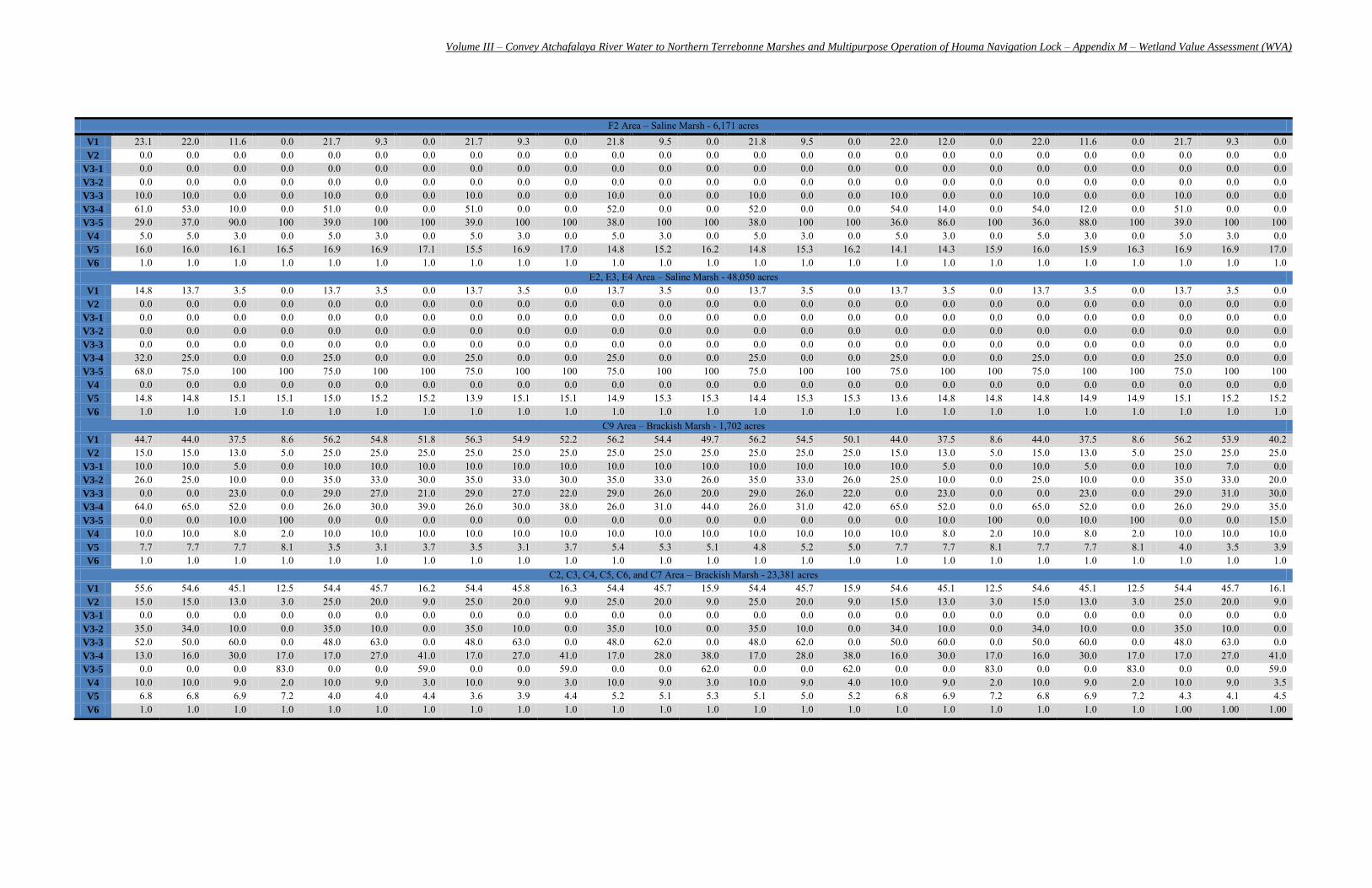
Volume III – Convey Atchafalaya River Water to Northern Terrebonne Marshes and Multipurpose Operation of Houma Navigation Lock – Appendix M – Wetland Value Assessment (WVA)
F2 Area – Saline Marsh - 6,171 acres
V1 23.1 22.0 11.6 0.0 21.7 9.3 0.0 21.7 9.3 0.0 21.8 9.5 0.0 21.8 9.5 0.0 22.0 12.0 0.0 22.0 11.6 0.0 21.7 9.3 0.0 V2 0.0 0.0 0.0 0.0 0.0 0.0 0.0 0.0 0.0 0.0 0.0 0.0 0.0 0.0 0.0 0.0 0.0 0.0 0.0 0.0 0.0 0.0 0.0 0.0 0.0
V3-1 0.0 0.0 0.0 0.0 0.0 0.0 0.0 0.0 0.0 0.0 0.0 0.0 0.0 0.0 0.0 0.0 0.0 0.0 0.0 0.0 0.0 0.0 0.0 0.0 0.0 V3-2 0.0 0.0 0.0 0.0 0.0 0.0 0.0 0.0 0.0 0.0 0.0 0.0 0.0 0.0 0.0 0.0 0.0 0.0 0.0 0.0 0.0 0.0 0.0 0.0 0.0 V3-3 10.0 10.0 0.0 0.0 10.0 0.0 0.0 10.0 0.0 0.0 10.0 0.0 0.0 10.0 0.0 0.0 10.0 0.0 0.0 10.0 0.0 0.0 10.0 0.0 0.0 V3-4 61.0 53.0 10.0 0.0 51.0 0.0 0.0 51.0 0.0 0.0 52.0 0.0 0.0 52.0 0.0 0.0 54.0 14.0 0.0 54.0 12.0 0.0 51.0 0.0 0.0 V3-5 29.0 37.0 90.0 100 39.0 100 100 39.0 100 100 38.0 100 100 38.0 100 100 36.0 86.0 100 36.0 88.0 100 39.0 100 100 V4 5.0 5.0 3.0 0.0 5.0 3.0 0.0 5.0 3.0 0.0 5.0 3.0 0.0 5.0 3.0 0.0 5.0 3.0 0.0 5.0 3.0 0.0 5.0 3.0 0.0 V5 16.0 16.0 16.1 16.5 16.9 16.9 17.1 15.5 16.9 17.0 14.8 15.2 16.2 14.8 15.3 16.2 14.1 14.3 15.9 16.0 15.9 16.3 16.9 16.9 17.0 V6 1.0 1.0 1.0 1.0 1.0 1.0 1.0 1.0 1.0 1.0 1.0 1.0 1.0 1.0 1.0 1.0 1.0 1.0 1.0 1.0 1.0 1.0 1.0 1.0 1.0
E2, E3, E4 Area – Saline Marsh - 48,050 acres V1 14.8 13.7 3.5 0.0 13.7 3.5 0.0 13.7 3.5 0.0 13.7 3.5 0.0 13.7 3.5 0.0 13.7 3.5 0.0 13.7 3.5 0.0 13.7 3.5 0.0 V2 0.0 0.0 0.0 0.0 0.0 0.0 0.0 0.0 0.0 0.0 0.0 0.0 0.0 0.0 0.0 0.0 0.0 0.0 0.0 0.0 0.0 0.0 0.0 0.0 0.0
V3-1 0.0 0.0 0.0 0.0 0.0 0.0 0.0 0.0 0.0 0.0 0.0 0.0 0.0 0.0 0.0 0.0 0.0 0.0 0.0 0.0 0.0 0.0 0.0 0.0 0.0 V3-2 0.0 0.0 0.0 0.0 0.0 0.0 0.0 0.0 0.0 0.0 0.0 0.0 0.0 0.0 0.0 0.0 0.0 0.0 0.0 0.0 0.0 0.0 0.0 0.0 0.0 V3-3 0.0 0.0 0.0 0.0 0.0 0.0 0.0 0.0 0.0 0.0 0.0 0.0 0.0 0.0 0.0 0.0 0.0 0.0 0.0 0.0 0.0 0.0 0.0 0.0 0.0 V3-4 32.0 25.0 0.0 0.0 25.0 0.0 0.0 25.0 0.0 0.0 25.0 0.0 0.0 25.0 0.0 0.0 25.0 0.0 0.0 25.0 0.0 0.0 25.0 0.0 0.0 V3-5 68.0 75.0 100 100 75.0 100 100 75.0 100 100 75.0 100 100 75.0 100 100 75.0 100 100 75.0 100 100 75.0 100 100 V4 0.0 0.0 0.0 0.0 0.0 0.0 0.0 0.0 0.0 0.0 0.0 0.0 0.0 0.0 0.0 0.0 0.0 0.0 0.0 0.0 0.0 0.0 0.0 0.0 0.0 V5 14.8 14.8 15.1 15.1 15.0 15.2 15.2 13.9 15.1 15.1 14.9 15.3 15.3 14.4 15.3 15.3 13.6 14.8 14.8 14.8 14.9 14.9 15.1 15.2 15.2 V6 1.0 1.0 1.0 1.0 1.0 1.0 1.0 1.0 1.0 1.0 1.0 1.0 1.0 1.0 1.0 1.0 1.0 1.0 1.0 1.0 1.0 1.0 1.0 1.0 1.0
C9 Area – Brackish Marsh - 1,702 acres V1 44.7 44.0 37.5 8.6 56.2 54.8 51.8 56.3 54.9 52.2 56.2 54.4 49.7 56.2 54.5 50.1 44.0 37.5 8.6 44.0 37.5 8.6 56.2 53.9 40.2 V2 15.0 15.0 13.0 5.0 25.0 25.0 25.0 25.0 25.0 25.0 25.0 25.0 25.0 25.0 25.0 25.0 15.0 13.0 5.0 15.0 13.0 5.0 25.0 25.0 25.0
V3-1 10.0 10.0 5.0 0.0 10.0 10.0 10.0 10.0 10.0 10.0 10.0 10.0 10.0 10.0 10.0 10.0 10.0 5.0 0.0 10.0 5.0 0.0 10.0 7.0 0.0 V3-2 26.0 25.0 10.0 0.0 35.0 33.0 30.0 35.0 33.0 30.0 35.0 33.0 26.0 35.0 33.0 26.0 25.0 10.0 0.0 25.0 10.0 0.0 35.0 33.0 20.0 V3-3 0.0 0.0 23.0 0.0 29.0 27.0 21.0 29.0 27.0 22.0 29.0 26.0 20.0 29.0 26.0 22.0 0.0 23.0 0.0 0.0 23.0 0.0 29.0 31.0 30.0 V3-4 64.0 65.0 52.0 0.0 26.0 30.0 39.0 26.0 30.0 38.0 26.0 31.0 44.0 26.0 31.0 42.0 65.0 52.0 0.0 65.0 52.0 0.0 26.0 29.0 35.0 V3-5 0.0 0.0 10.0 100 0.0 0.0 0.0 0.0 0.0 0.0 0.0 0.0 0.0 0.0 0.0 0.0 0.0 10.0 100 0.0 10.0 100 0.0 0.0 15.0 V4 10.0 10.0 8.0 2.0 10.0 10.0 10.0 10.0 10.0 10.0 10.0 10.0 10.0 10.0 10.0 10.0 10.0 8.0 2.0 10.0 8.0 2.0 10.0 10.0 10.0 V5 7.7 7.7 7.7 8.1 3.5 3.1 3.7 3.5 3.1 3.7 5.4 5.3 5.1 4.8 5.2 5.0 7.7 7.7 8.1 7.7 7.7 8.1 4.0 3.5 3.9 V6 1.0 1.0 1.0 1.0 1.0 1.0 1.0 1.0 1.0 1.0 1.0 1.0 1.0 1.0 1.0 1.0 1.0 1.0 1.0 1.0 1.0 1.0 1.0 1.0 1.0
C2, C3, C4, C5, C6, and C7 Area – Brackish Marsh - 23,381 acres V1 55.6 54.6 45.1 12.5 54.4 45.7 16.2 54.4 45.8 16.3 54.4 45.7 15.9 54.4 45.7 15.9 54.6 45.1 12.5 54.6 45.1 12.5 54.4 45.7 16.1 V2 15.0 15.0 13.0 3.0 25.0 20.0 9.0 25.0 20.0 9.0 25.0 20.0 9.0 25.0 20.0 9.0 15.0 13.0 3.0 15.0 13.0 3.0 25.0 20.0 9.0
V3-1 0.0 0.0 0.0 0.0 0.0 0.0 0.0 0.0 0.0 0.0 0.0 0.0 0.0 0.0 0.0 0.0 0.0 0.0 0.0 0.0 0.0 0.0 0.0 0.0 0.0 V3-2 35.0 34.0 10.0 0.0 35.0 10.0 0.0 35.0 10.0 0.0 35.0 10.0 0.0 35.0 10.0 0.0 34.0 10.0 0.0 34.0 10.0 0.0 35.0 10.0 0.0 V3-3 52.0 50.0 60.0 0.0 48.0 63.0 0.0 48.0 63.0 0.0 48.0 62.0 0.0 48.0 62.0 0.0 50.0 60.0 0.0 50.0 60.0 0.0 48.0 63.0 0.0 V3-4 13.0 16.0 30.0 17.0 17.0 27.0 41.0 17.0 27.0 41.0 17.0 28.0 38.0 17.0 28.0 38.0 16.0 30.0 17.0 16.0 30.0 17.0 17.0 27.0 41.0 V3-5 0.0 0.0 0.0 83.0 0.0 0.0 59.0 0.0 0.0 59.0 0.0 0.0 62.0 0.0 0.0 62.0 0.0 0.0 83.0 0.0 0.0 83.0 0.0 0.0 59.0 V4 10.0 10.0 9.0 2.0 10.0 9.0 3.0 10.0 9.0 3.0 10.0 9.0 3.0 10.0 9.0 4.0 10.0 9.0 2.0 10.0 9.0 2.0 10.0 9.0 3.5 V5 6.8 6.8 6.9 7.2 4.0 4.0 4.4 3.6 3.9 4.4 5.2 5.1 5.3 5.1 5.0 5.2 6.8 6.9 7.2 6.8 6.9 7.2 4.3 4.1 4.5 V6 1.0 1.0 1.0 1.0 1.0 1.0 1.0 1.0 1.0 1.0 1.0 1.0 1.0 1.0 1.0 1.0 1.0 1.0 1.0 1.0 1.0 1.0 1.00 1.00 1.00
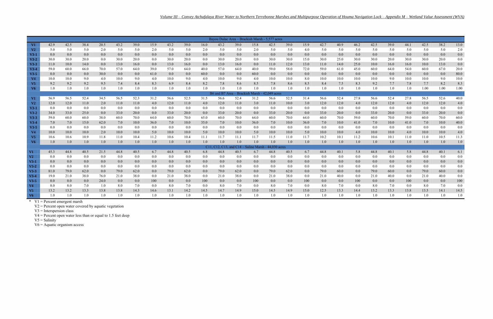
Volume III – Convey Atchafalaya River Water to Northern Terrebonne Marshes and Multipurpose Operation of Houma Navigation Lock – Appendix M – Wetland Value Assessment (WVA)
* V1 = Percent emergent marsh V2 = Percent open water covered by aquatic vegetation V3 = Interspersion class V4 = Percent open water less than or equal to 1.5 feet deep V5 = Salinity V6 = Aquatic organism access
Bayou Dulac Area – Brackish Marsh - 5,577 acres V1 42.9 42.5 38.4 20.5 43.2 39.0 15.9 43.2 39.0 16.0 43.2 39.0 15.8 42.5 39.0 15.9 42.7 40.9 46.2 42.5 39.0 44.1 42.5 38.2 13.0 V2 5.0 5.0 5.0 2.0 5.0 5.0 2.0 5.0 5.0 2.0 5.0 5.0 2.0 5.0 5.0 4.0 5.0 5.0 5.0 5.0 5.0 5.0 5.0 5.0 2.0
V3-1 0.0 0.0 0.0 0.0 0.0 0.0 0.0 0.0 0.0 0.0 0.0 0.0 0.0 0.0 0.0 0.0 0.0 0.0 0.0 0.0 0.0 0.0 0.0 0.0 0.0 V3-2 30.0 30.0 20.0 0.0 30.0 20.0 0.0 30.0 20.0 0.0 30.0 20.0 0.0 30.0 30.0 15.0 30.0 25.0 30.0 30.0 20.0 30.0 30.0 20.0 0.0 V3-3 11.0 10.0 14.0 0.0 13.0 16.0 0.0 13.0 16.0 0.0 13.0 16.0 0.0 11.0 12.0 13.0 11.0 14.0 25.0 10.0 16.0 16.0 10.0 13.0 0.0 V3-4 59.0 60.0 66.0 70.0 57.0 64.0 39.0 57.0 64.0 40.0 57.0 64.0 40.0 59.0 58.0 72.0 59.0 61.0 45.0 60.0 64.0 54.0 60.0 67.0 20.0 V3-5 0.0 0.0 0.0 30.0 0.0 0.0 61.0 0.0 0.0 60.0 0.0 0.0 60.0 0.0 0.0 0.0 0.0 0.0 0.0 0.0 0.0 0.0 0.0 0.0 80.0 V4 10.0 10.0 9.0 4.0 10.0 9.0 4.0 10.0 9.0 4.0 10.0 9.0 4.0 10.0 10.0 8.0 10.0 10.0 10.0 10.0 9.0 10.0 10.0 9.0 10.0 V5 9.2 9.2 9.2 9.5 7.4 8.4 8.3 6.9 8.4 8.2 7.8 8.6 8.5 7.8 8.6 8.5 8.4 7.5 8.3 9.2 7.7 7.8 7.7 8.2 8.3 V6 1.0 1.0 1.0 1.0 1.0 1.0 1.0 1.0 1.0 1.0 1.0 1.0 1.0 1.0 1.0 1.0 1.0 1.0 1.0 1.0 1.0 1.0 1.00 1.00 1.00
B6 and B7 Area – Brackish Marsh - 42,049 acres V1 56.9 56.5 52.4 34.5 56.5 52.3 31.2 56.6 52.5 31.5 56.6 52.4 31.2 56.6 52.5 31.4 56.6 52.4 27.8 56.6 52.4 27.8 56.5 52.6 40.0 V2 12.0 12.0 11.0 2.0 11.0 11.0 4.0 12.0 11.0 4.0 12.0 11.0 3.0 11.0 10.0 3.0 12.0 12.0 4.0 12.0 12.0 4.0 12.0 12.0 4.0
V3-1 0.0 0.0 0.0 0.0 0.0 0.0 0.0 0.0 0.0 0.0 0.0 0.0 0.0 0.0 0.0 0.0 0.0 0.0 0.0 0.0 0.0 0.0 0.0 0.0 0.0 V3-2 34.0 33.0 25.0 0.0 33.0 20.0 0.0 33.0 20.0 0.0 33.0 20.0 0.0 33.0 20.0 0.0 33.0 20.0 0.0 33.0 20.0 0.0 33.0 20.0 0.0 V3-3 59.0 60.0 60.0 38.0 60.0 70.0 64.0 60.0 70.0 65.0 60.0 70.0 64.0 60.0 70.0 64.0 60.0 70.0 59.0 60.0 70.0 59.0 60.0 70.0 60.0 V3-4 7.0 7.0 15.0 62.0 7.0 10.0 36.0 7.0 10.0 35.0 7.0 10.0 36.0 7.0 10.0 36.0 7.0 10.0 41.0 7.0 10.0 41.0 7.0 10.0 40.0 V3-5 0.0 0.0 0.0 0.0 0.0 0.0 0.0 0.0 0.0 0.0 0.0 0.0 0.0 0.0 0.0 0.0 0.0 0.0 0.0 0.0 0.0 0.0 0.0 0.0 0.0 V4 10.0 10.0 10.0 2.0 10.0 10.0 5.0 10.0 10.0 5.0 10.0 10.0 5.0 10.0 10.0 5.0 10.0 10.0 4.0 10.0 10.0 4.0 10.0 10.0 4.0 V5 10.6 10.6 10.9 11.8 11.0 10.4 11.2 10.6 10.4 11.1 11.7 11.1 11.7 11.5 11.0 11.7 10.2 10.1 11.2 10.6 10.1 11.0 11.0 10.5 11.3 V6 1.0 1.0 1.0 1.0 1.0 1.0 1.0 1.0 1.0 1.0 1.0 1.0 1.0 1.0 1.0 1.0 1.0 1.0 1.0 1.0 1.0 1.0 1.0 1.0 1.0
C11, C12, C13, and C14 – Saline Marsh - 44,030 acres V1 45.3 44.8 40.5 21.5 44.8 40.5 6.7 44.8 40.5 6.8 44.8 40.5 6.7 44.8 40.5 6.7 44.8 40.1 5.8 44.8 40.1 5.8 44.8 40.1 6.1 V2 0.0 0.0 0.0 0.0 0.0 0.0 0.0 0.0 0.0 0.0 0.0 0.0 0.0 0.0 0.0 0.0 0.0 0.0 0.0 0.0 0.0 0.0 0.0 0.0 0.0 V3-1 0.0 0.0 0.0 0.0 0.0 0.0 0.0 0.0 0.0 0.0 0.0 0.0 0.0 0.0 0.0 0.0 0.0 0.0 0.0 0.0 0.0 0.0 0.0 0.0 0.0 V3-2 0.0 0.0 0.0 0.0 0.0 0.0 0.0 0.0 0.0 0.0 0.0 0.0 0.0 0.0 0.0 0.0 0.0 0.0 0.0 0.0 0.0 0.0 0.0 0.0 0.0 V3-3 81.0 79.0 62.0 0.0 79.0 62.0 0.0 79.0 62.0 0.0 79.0 62.0 0.0 79.0 62.0 0.0 79.0 60.0 0.0 79.0 60.0 0.0 79.0 60.0 0.0 V3-4 19.0 21.0 38.0 76.0 21.0 38.0 0.0 21.0 38.0 0.0 21.0 38.0 0.0 21.0 38.0 0.0 21.0 40.0 0.0 21.0 40.0 0.0 21.0 40.0 0.0 V3-5 0.0 0.0 0.0 24.0 0.0 0.0 100 0.0 0.0 100 0.0 0.0 100 0.0 0.0 100 0.0 0.0 100 0.0 0.0 100 0.0 0.0 100 V4 8.0 8.0 7.0 1.0 8.0 7.0 0.0 8.0 7.0 0.0 8.0 7.0 0.0 8.0 7.0 0.0 8.0 7.0 0.0 8.0 7.0 0.0 8.0 7.0 0.0 V5 13.2 13.2 13.3 13.8 13.8 14.3 14.6 13.1 14.2 14.5 14.7 14.9 15.0 14.5 14.9 15.0 12.5 13.3 14.4 13.2 13.3 13.8 13.5 14.1 14.5 V6 1.0 1.0 1.0 1.0 1.0 1.0 1.0 1.0 1.0 1.0 1.0 1.0 1.0 1.0 1.0 1.0 1.0 1.0 1.0 1.0 1.0 1.0 1.0 1.0 1.0
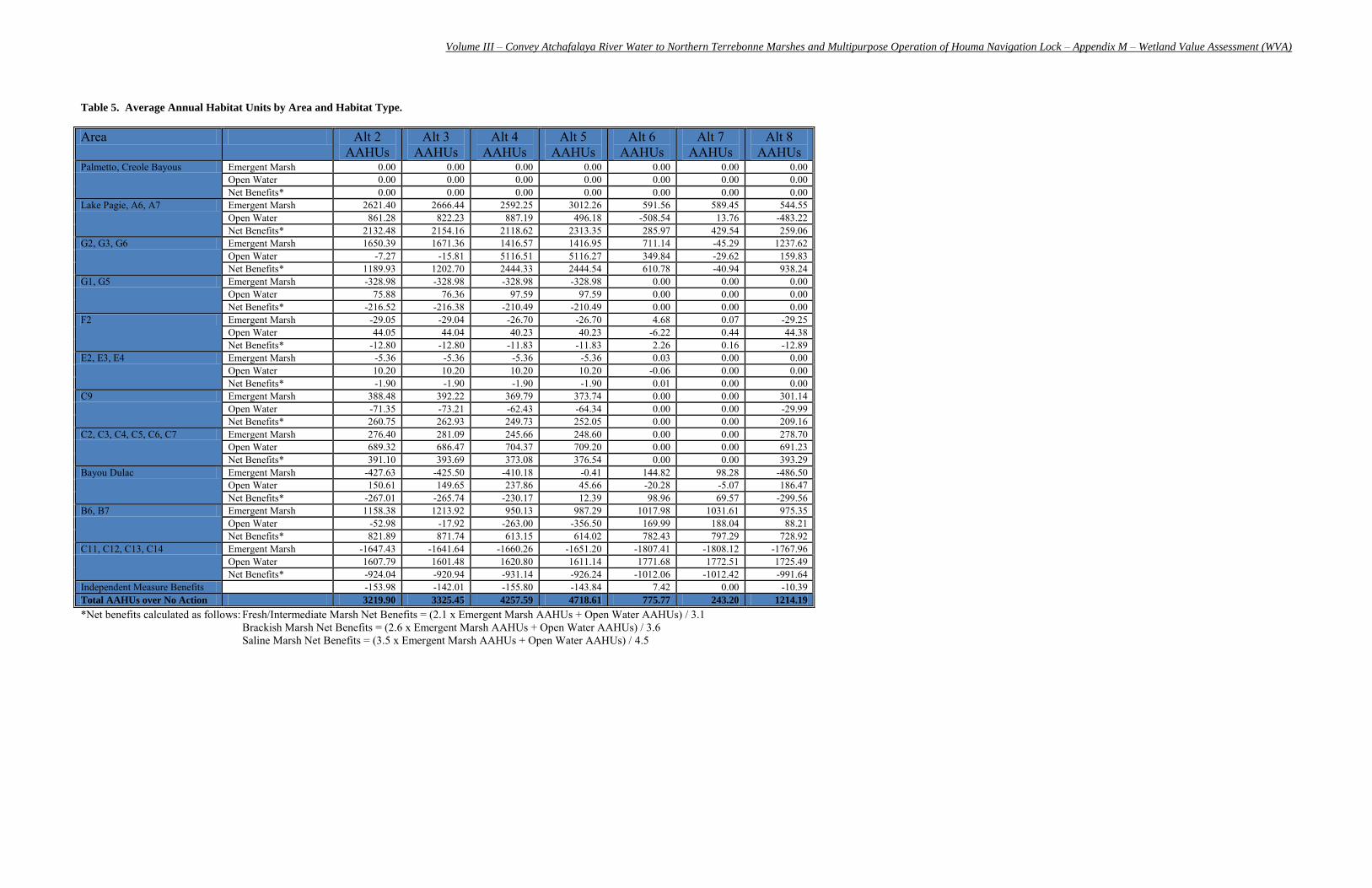
Volume III – Convey Atchafalaya River Water to Northern Terrebonne Marshes and Multipurpose Operation of Houma Navigation Lock – Appendix M – Wetland Value Assessment (WVA)
Table 5. Average Annual Habitat Units by Area and Habitat Type.
Area Alt 2 AAHUs
Alt 3 AAHUs
Alt 4 AAHUs
Alt 5 AAHUs
Alt 6 AAHUs
Alt 7 AAHUs
Alt 8 AAHUs
Palmetto, Creole Bayous Emergent Marsh 0.00 0.00 0.00 0.00 0.00 0.00 0.00 Open Water 0.00 0.00 0.00 0.00 0.00 0.00 0.00 Net Benefits* 0.00 0.00 0.00 0.00 0.00 0.00 0.00
Lake Pagie, A6, A7 Emergent Marsh 2621.40 2666.44 2592.25 3012.26 591.56 589.45 544.55 Open Water 861.28 822.23 887.19 496.18 -508.54 13.76 -483.22 Net Benefits* 2132.48 2154.16 2118.62 2313.35 285.97 429.54 259.06
G2, G3, G6 Emergent Marsh 1650.39 1671.36 1416.57 1416.95 711.14 -45.29 1237.62 Open Water -7.27 -15.81 5116.51 5116.27 349.84 -29.62 159.83 Net Benefits* 1189.93 1202.70 2444.33 2444.54 610.78 -40.94 938.24
G1, G5 Emergent Marsh -328.98 -328.98 -328.98 -328.98 0.00 0.00 0.00 Open Water 75.88 76.36 97.59 97.59 0.00 0.00 0.00 Net Benefits* -216.52 -216.38 -210.49 -210.49 0.00 0.00 0.00
F2 Emergent Marsh -29.05 -29.04 -26.70 -26.70 4.68 0.07 -29.25 Open Water 44.05 44.04 40.23 40.23 -6.22 0.44 44.38 Net Benefits* -12.80 -12.80 -11.83 -11.83 2.26 0.16 -12.89
E2, E3, E4 Emergent Marsh -5.36 -5.36 -5.36 -5.36 0.03 0.00 0.00 Open Water 10.20 10.20 10.20 10.20 -0.06 0.00 0.00 Net Benefits* -1.90 -1.90 -1.90 -1.90 0.01 0.00 0.00
C9 Emergent Marsh 388.48 392.22 369.79 373.74 0.00 0.00 301.14 Open Water -71.35 -73.21 -62.43 -64.34 0.00 0.00 -29.99 Net Benefits* 260.75 262.93 249.73 252.05 0.00 0.00 209.16
C2, C3, C4, C5, C6, C7 Emergent Marsh 276.40 281.09 245.66 248.60 0.00 0.00 278.70 Open Water 689.32 686.47 704.37 709.20 0.00 0.00 691.23 Net Benefits* 391.10 393.69 373.08 376.54 0.00 0.00 393.29
Bayou Dulac Emergent Marsh -427.63 -425.50 -410.18 -0.41 144.82 98.28 -486.50 Open Water 150.61 149.65 237.86 45.66 -20.28 -5.07 186.47 Net Benefits* -267.01 -265.74 -230.17 12.39 98.96 69.57 -299.56
B6, B7 Emergent Marsh 1158.38 1213.92 950.13 987.29 1017.98 1031.61 975.35 Open Water -52.98 -17.92 -263.00 -356.50 169.99 188.04 88.21 Net Benefits* 821.89 871.74 613.15 614.02 782.43 797.29 728.92
C11, C12, C13, C14 Emergent Marsh -1647.43 -1641.64 -1660.26 -1651.20 -1807.41 -1808.12 -1767.96 Open Water 1607.79 1601.48 1620.80 1611.14 1771.68 1772.51 1725.49 Net Benefits* -924.04 -920.94 -931.14 -926.24 -1012.06 -1012.42 -991.64
Independent Measure Benefits -153.98 -142.01 -155.80 -143.84 7.42 0.00 -10.39 Total AAHUs over No Action 3219.90 3325.45 4257.59 4718.61 775.77 243.20 1214.19
*Net benefits calculated as follows: Fresh/Intermediate Marsh Net Benefits = (2.1 x Emergent Marsh AAHUs + Open Water AAHUs) / 3.1 Brackish Marsh Net Benefits = (2.6 x Emergent Marsh AAHUs + Open Water AAHUs) / 3.6 Saline Marsh Net Benefits = (3.5 x Emergent Marsh AAHUs + Open Water AAHUs) / 4.5