appendix c4: design of sailplanes - elsevier · the modern sailplane features a tadpole fuselage,...

GUDMUNDSSON – GENERAL AVIATION AIRCRAFT DESIGN APPENDIX C4 – DESIGN OF SAILPLANES 1

©2013 Elsevier, Inc. This material may not be copied or distributed without permission from the Publisher.

APPENDIX C4: Design of Sailplanes

This appendix is a part of the book General Aviation

Aircraft Design: Applied Methods and Procedures by

Snorri Gudmundsson, published by Elsevier, Inc. The book

is available through various bookstores and online

retailers, such as www.elsevier.com, www.amazon.com,

and many others.

The purpose of the appendices denoted by C1 through C5

is to provide additional information on the design of

selected aircraft configurations, beyond what is possible in

the main part of Chapter 4, Aircraft Conceptual Layout.

Some of the information is intended for the novice

engineer, but other is advanced and well beyond what is

possible to present in undergraduate design classes. This

way, the appendices can serve as a refresher material for

the experienced aircraft designer, while introducing new

material to the student. Additionally, many helpful design

philosophies are presented in the text. Since this appendix

is offered online rather than in the actual book, it is

possible to revise it regularly and both add to the

information and new types of aircraft. The following

appendices are offered:

C1 – Design of Conventional Aircraft

C2 – Design of Canard Aircraft

C3 – Design of Seaplanes

C4 – Design of Sailplanes (this appendix)

C5 – Design of Unusual Configurations

Figure C4-1: A Rolladen-Schneider LS-4 sailplane touching down using standard tail-first technique. Note the

deployed spoilers on the upper surface of the wing. The sleekness of sailplanes would make them very hard to

land were it not for spoilers that allow the drag to be increased temporarily during approach to landing,

enabling standard approach angles to be used. (Photo by Phil Rademacher)



C4.1 Design of Sailplanes

Flying sailplanes and gliders remains a very popular past-time for many people. Gliding is the oldest form of

heavier than air flight, dating back to the days of Otto Lilienthal (1848-1896) who pioneered the craft. For many,

the absence of power offers incomparable simplicity and purity that allows the aviator to experience what it is to

fly like the birds. However, the apparent simplicity is a veil that covers a level of design sophistication far superior

to most GA aircraft. This appendix scratches the surface of conceptual design of sailplanes.

C4.1.1 Sailplane Fundamentals

Configuration A in Figure C4-2 presents an example of what the typical modern sailplane looks like. No aircraft

generate less drag than sailplanes; their efficiency is a marvel of engineering. Configuration B is an example of a

long endurance UAV, which “borrows” many sailplane features. The typical sailplane carries one to two people, it

has a gross weight ranging from 800 to 1800 lbf, wingspan from 35 to 101 ft, wing Aspect Ratio from 10 to 51, and

wing loading from 5-12 lbf/ft². At this time, the largest sailplane in the world is the German built Eta, with a

wingspan of 101 ft, AR of 51, and wing loading of 10.44 lbf/ft². It is thought to have a glide ratio around 70 – this

means a glide path angle of 0.8° - or a still air glide range of 115 nm from an altitude of 10000 ft. Today, serious

sailplanes are only fabricated using composite materials that yield the smoothest aerodynamic surfaces possible.

Figure C4-2: A sailplane (A) and a powered sailplane used as a UAV (B).

The modern sailplane features a tadpole fuselage, whose forward section is shaped to sustain laminar boundary

layer naturally (Natural Laminar Flow or NLF) and contracted tail-boom to minimize the wetted area1, once the

boundary layer has transitioned into turbulent one. The fuselage is shaped to minimize the frontal area of the

vehicle, but this requires the pilot to sit in an inclined position. More efficient sailplanes use a single piece canopy,

which allows the NLF to extend farther aft on the fuselage than a two piece one. The modern sailplane uses a

Schumann style wing planform (see Section 9.2.2, The Schuemann Wing) so its section lift distribution better

resembles that of the harder to manufacture elliptical wing planform. Sometimes polyhedral dihedral is employed

to reduce lift-induced drag further (see Section 10.5.9, The Polyhedral Wing(tip)). The most significant contributor

to the low drag properties of sailplanes is its wing, and horizontal and vertical tails, all which feature NLF airfoils.

Sailplanes usually utilize T-tails to place the HT outside of the turbulent wake of the fuselage. This helps sustaining

a stable NLF over its surface. Section C4.1.4, Sailplane Tail Design presents a method to help with the sizing and

positioning of the HT.

Operation of Sailplanes

Sailplanes demand a lot from their operators and proper flying techniques require extensive pilot training. Pilots

must know how best to position the sailplane “on tow”, how to develop “feel” when searching for lift, how to get

the most out of thermals, and how best to manage approach and landing, considering the lack of power reduces

the room for error2. This requires the pilot to spend long hours sharpening these skills, sitting inclined in a tiny

cockpit. For this reason, the sailplane designer must be mindful of cockpit ergonomics, in addition to other factors

(performance, stability, transportation, maintenance, etc.).



Sailplanes are designed to offer the largest glide ratio possible and, ideally, this should be attainable at high

airspeed (something that requires an extensive drag bucket, cruise flaps, or jettisonable water ballast). Their

exceedingly low rate of descent allows them to stay aloft for long periods, provided atmospheric convection is

present. This is possible because even the most anemic atmospheric convection rises faster than the rate of

descent for such vehicles.

Sailplane pilots take advantage of four kinds of convection (rising air); thermals, ridge lift, standing mountain

waves, and convergence lift. Sailplane pilots refer to these as lift. A thermal is a column of rising air due to the

ground being heated by the sun. The warmer air is less dense than the surrounding air, causing it to rise. Thermals

can reach altitudes as high as 18000 ft, although 5000-6000 ft is more common. Thermals can often be identified

by the cumulus clouds that reside on top of them. Ridge lift results from wind being forced over ground features,

such as cliffs, mountains, and ridges. Wave lift is the consequence of oscillatory motion of air, referred to as gravity

waves by atmospheric scientists. Sailplanes have reached altitudes in the upper 40000 ft while utilizing such lift.

For instance, the cited altitude record below was achieved in such a wave. Convergence lift occurs when two

masses of air collide, such as sea-breeze and inland air mass.

In addition to these, a gliding technique called dynamic soaring can be employed provided certain atmospheric

conditions prevail. These are characterized by two air masses moving at different rates while being separated by a

thin shear layer; a fictitious layer characterized by rapid change in wind speed. Such conditions typically exist near

the ground between valleys of ocean waves or on the leeward side of ridges. The wind speed in the upper air mass

is much greater when compared to the lower one and the two are separated by a steep speed gradient. The actual

dynamic soaring consists of a set of maneuvers intended to systematically exchange kinetic and potential energy

and make up for the energy lost to drag, by taking advantage of the gain in ground speed as the vehicle flies

downwind (see Figure C4-3). This way, at 1, the sailplane turns into the wind direction, still below the shear layer

where the wind speed is negligible. At 2 it has begun a climb that will take it through the shear layer, where the

headwind will now increase rapidly. The true airspeed and, thus, the dynamic pressure acting on the vehicle rise

sharply as its inertia drives it through the oncoming wind flow. The rise of lift is instantly transformed into climb to

a higher altitude. At the same time, its airspeed is reduced gradually. To prevent too much loss in airspeed, the

vehicle banks sharply at 3 and begins a dive toward the ground with the wind becoming a tailwind. At 4, the

vehicle penetrates the shear layer again, now having accelerated with respect to the ground thanks to the tailwind.

At 5, the vehicle begins a new bank to change the heading into the wind and repeat the cycle.

Figure C4-3: The basics of dynamic soaring.



Dynamic soaring is utilized by many species of seabirds, some which use it to travel great distances. However, no

bird species rivals the Albatross, who regularly travel thousands of miles in a single trip, with minimal flapping of

the wings, effectively gliding across oceans. Among humans, the method is used both among pilots of sailplanes

and radio-controlled aircraft.

Long distance flying in sailplanes simply involves taking advantage of the energy available in the atmosphere that

can be used to maintain necessary altitude. The pilot will ride the lift as high as possible before proceeding to the

next source of rising air. As such, the typical cross-country sailplane flight consists of a climb, followed by a

descent, followed by another climb, and so forth. It is possible to reach very high altitudes in the process. Altitudes

exceeding 30000 ft is a common occurrence and certainly requires an oxygen bottle to be carried along. The

current altitude record in a sailplane is 50722 ft (15460 m), set on 29th

of August, 2006 by the Americans Steve

Fossett (1944-2007) and Einar Enevoldson, in a modified Glaser-Dirks DG-505 Open Class sailplane3. The current

long range record stands at about 1214 nm (2248 km), set by Klaus Ohlman on 2nd

of December, 2003, on a

Schempp-Hirth Nimbus Open Class sailplane4.

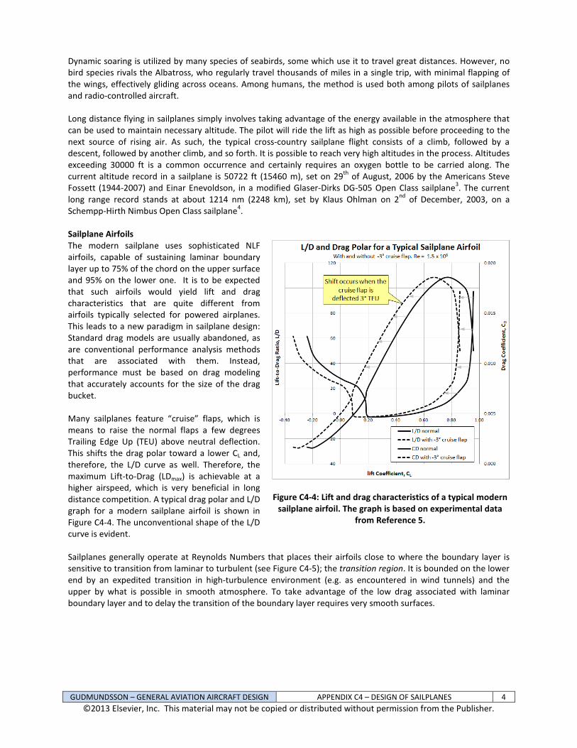
Sailplane Airfoils

The modern sailplane uses sophisticated NLF

airfoils, capable of sustaining laminar boundary

layer up to 75% of the chord on the upper surface

and 95% on the lower one. It is to be expected

that such airfoils would yield lift and drag

characteristics that are quite different from

airfoils typically selected for powered airplanes.

This leads to a new paradigm in sailplane design:

Standard drag models are usually abandoned, as

are conventional performance analysis methods

that are associated with them. Instead,

performance must be based on drag modeling

that accurately accounts for the size of the drag

bucket.

Many sailplanes feature “cruise” flaps, which is

means to raise the normal flaps a few degrees

Trailing Edge Up (TEU) above neutral deflection.

This shifts the drag polar toward a lower CL and,

therefore, the L/D curve as well. Therefore, the

maximum Lift-to-Drag (LDmax) is achievable at a

higher airspeed, which is very beneficial in long

distance competition. A typical drag polar and L/D

graph for a modern sailplane airfoil is shown in

Figure C4-4. The unconventional shape of the L/D

curve is evident.

Figure C4-4: Lift and drag characteristics of a typical modern

sailplane airfoil. The graph is based on experimental data

from Reference 5.

Sailplanes generally operate at Reynolds Numbers that places their airfoils close to where the boundary layer is

sensitive to transition from laminar to turbulent (see Figure C4-5); the transition region. It is bounded on the lower

end by an expedited transition in high-turbulence environment (e.g. as encountered in wind tunnels) and the

upper by what is possible in smooth atmosphere. To take advantage of the low drag associated with laminar

boundary layer and to delay the transition of the boundary layer requires very smooth surfaces.



Figure C4-5: Sailplanes operate in the transition region and must feature smooth surfaces to delay transition

from laminar to turbulent boundary layer. (Adapted from Reference 6)

The Importance of the Drag Bucket

Figure C4-6 is an idealized representation

intended to show the importance of

achieving NLF on a hypothetical sailplane.

The shape of both the drag polar and L/D

curve is classical for all NLF airfoils that

feature a distinct two-wall drag bucket,

including the double peak shape of the L/D

curve. For instance, this characteristic is

present in most NACA 65- and 66-series

airfoils. The figure shows the impact this has

on the glide performance of a hypothetical

sailplane. Reducing the CDmin by 30 drag

counts (e.g. from 0.013 to 0.010) increases

the maximum L/D ratio by 4.2 units and

shifts its location to a much lower CL. Lower

CL means the LDmax will be realized at higher

airspeed; something very beneficial to a

sailplane (and would be to a powered cruiser

as well). Admittedly 30 drag counts are on

the high end of drag reduction and often the

drag characteristics of the airplane as a

whole mask the presence of the drag bucket,

so a distinct double-peak LD curves is not

always achieved for many applications.

Instead, the laminar bucket shifts or widens

the range of CL, where “near” LDmax

performance is found.

Figure C4-6: Example of the benefit of achieving NLF on a

hypothetical sailplane.



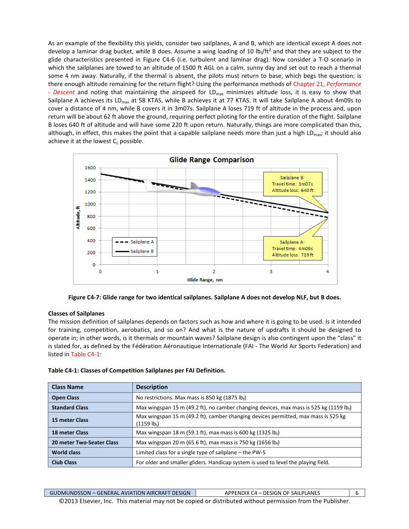
As an example of the flexibility this yields, consider two sailplanes, A and B, which are identical except A does not

develop a laminar drag bucket, while B does. Assume a wing loading of 10 lbf/ft² and that they are subject to the

glide characteristics presented in Figure C4-6 (i.e. turbulent and laminar drag). Now consider a T-O scenario in

which the sailplanes are towed to an altitude of 1500 ft AGL on a calm, sunny day and set out to reach a thermal

some 4 nm away. Naturally, if the thermal is absent, the pilots must return to base, which begs the question; is

there enough altitude remaining for the return flight? Using the performance methods of Chapter 21, Performance

- Descent and noting that maintaining the airspeed for LDmax minimizes altitude loss, it is easy to show that

Sailplane A achieves its LDmax at 58 KTAS, while B achieves it at 77 KTAS. It will take Sailplane A about 4m09s to

cover a distance of 4 nm, while B covers it in 3m07s. Sailplane A loses 719 ft of altitude in the process and, upon

return will be about 62 ft above the ground, requiring perfect piloting for the entire duration of the flight. Sailplane

B loses 640 ft of altitude and will have some 220 ft upon return. Naturally, things are more complicated than this,

although, in effect, this makes the point that a capable sailplane needs more than just a high LDmax; it should also

achieve it at the lowest CL possible.

Figure C4-7: Glide range for two identical sailplanes. Sailplane A does not develop NLF, but B does.

Classes of Sailplanes

The mission definition of sailplanes depends on factors such as how and where it is going to be used. Is it intended

for training, competition, aerobatics, and so on? And what is the nature of updrafts it should be designed to

operate in; in other words, is it thermals or mountain waves? Sailplane design is also contingent upon the “class” it

is slated for, as defined by the Fédération Aéronautique Internationale (FAI - The World Air Sports Federation) and

listed in Table C4-1:

Table C4-1: Classes of Competition Sailplanes per FAI Definition.

Class Name Description

Open Class No restrictions. Max mass is 850 kg (1875 lbf)

Standard Class Max wingspan 15 m (49.2 ft), no camber changing devices, max mass is 525 kg (1159 lbf)

15 meter Class Max wingspan 15 m (49.2 ft), camber changing devices permitted, max mass is 525 kg

(1159 lbf)

18 meter Class Max wingspan 18 m (59.1 ft), max mass is 600 kg (1325 lbf)

20 meter Two-Seater Class Max wingspan 20 m (65.6 ft), max mass is 750 kg (1656 lbf)

World class Limited class for a single type of sailplane – the PW-5

Club Class For older and smaller gliders. Handicap system is used to level the playing field.



C4.1.2 Sailplane Glide Performance

Since the standard operation of sailplanes excludes the use of power (self-launching sailplanes glide with engine

power off), their flight is far more influenced by the presence of rising and sinking air, as well as head- and

tailwinds. A deep understanding of glide performance is imperative for sailplane pilots, in particular when

attempting to maximize range. This section focuses on a few important elements of glide performance. It is largely

based on references such as Reichmann7, Welch and Irving

2, Thomas

6, Stewart

8, and Scull

9. In order to help explain

the fundamentals of glide performance, the properties of Sailplane A, discussed above, will be utilized in the

following discussion. To keep things manageable, a simplified quadratic drag model is used, given by CD = 0.010 +

0.01498∙CL². Also, time is represented using a format in which 6.25 minutes would be written as 6m15s.

Glide Range and Glide Endurance

The glide range is the horizontal distance a gliding aircraft covers between two given altitudes. The maximum

range in still air is obtained by maintaining the airspeed for minimum glide angle (or best angle of descent),

denoted by VBG. The glide endurance is the time that takes a gliding aircraft to descent between two given

altitudes. The maximum endurance in still air is obtained maintaining the airspeed for minimum rate of descent,

denoted by VBA. This is shown schematically in Figure C4-8.

Figure C4-8: A simple schematic showing the impact of any particular airspeed on glide range and time aloft of

Sailplane A, from an altitude of 1000 ft, assuming still air. In still air, VBG always yields the longest range and VBA

the longest time aloft. Values are obtained using a flight polar like the one in Figure C4-9.

Basic Mathematical Relations for Glide Performance

The following expressions are derived in Chapter 21, Performance – Descent and are repeated here for

convenience. All assume pure unpowered glide in still air and the simplified drag model.

Angle of descent: W

D

DLL

D≈==θ

/

1tan (21-8)

Rate of descent: ( )DL

VCC

V

W

DVV == (21-10)

Rate of descent: ( ) S

W

C

C

S

W

CCV

L

D

DL

Vρ

=ρ

=22

2323 (21-12)

Sink rate while banking at φ : ( )( ) S

W

C

C

S

W

CCV

L

D

DL

Vρφ

=φρ

=2

coscos

2232323

(21-13)



Equilibrium glide speed S

W

CV

Lρ

θ=

cos2 (21-11)

Airspeed of Minimum Sink Rate:

min3

2

D

BAC

k

S

WV

⋅

ρ= (21-14)

Minimum Angle-of-Descent: min

max

min 41

tan DCkLD

⋅⋅==θ (21-15)

Best glide speed (still air): S

W

C

kVV

D

LDBG

min

max

2

ρ== (21-16)

Glide range:

⋅=

⋅=

D

Lglide

C

Ch

D

LhR (21-17)

Where: CD = Drag coefficient

CDmin = Minimum drag coefficient

CL = Lift coefficient

D = Drag

h = Altitude

k = Lift-induced drag constant

L = Lift

LDmax = Maximum lift-to-drag ratio

Rglide = Glide range

S = Reference wing area

V = Airspeed

VBA = Airspeed of minimum rate of descent

VBG = Airspeed of best glide (where LDmax occurs)

VV = Vertical airspeed

W = Weight

φ = Bank angle

θ = Glide angle

θmin = Minimum glide angle

ρ = Air density

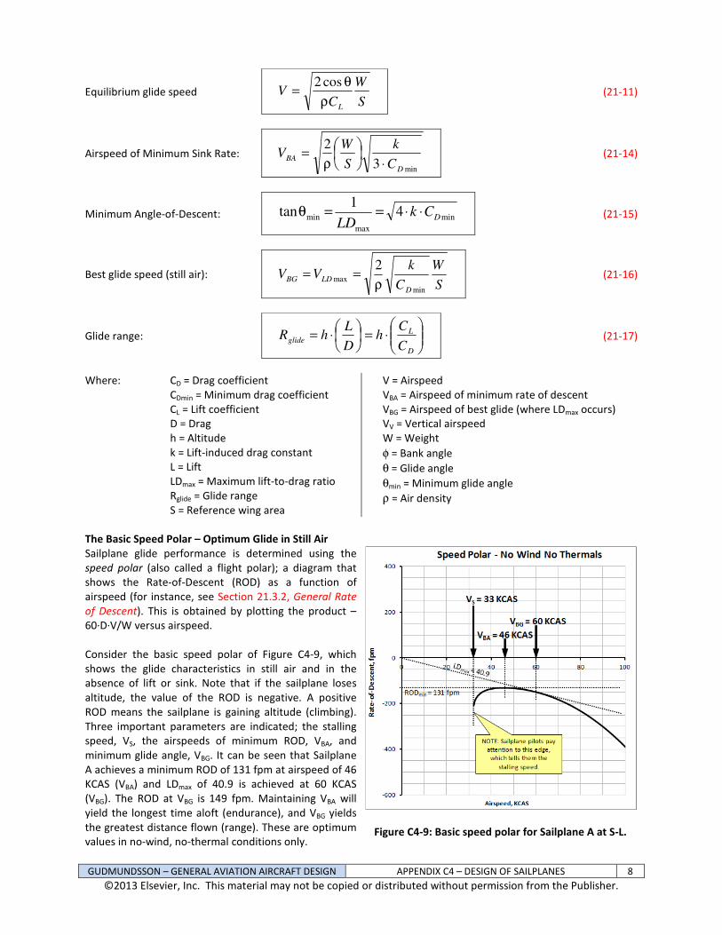
The Basic Speed Polar – Optimum Glide in Still Air

Sailplane glide performance is determined using the

speed polar (also called a flight polar); a diagram that

shows the Rate-of-Descent (ROD) as a function of

airspeed (for instance, see Section 21.3.2, General Rate

of Descent). This is obtained by plotting the product –

60∙D∙V/W versus airspeed.

Consider the basic speed polar of Figure C4-9, which

shows the glide characteristics in still air and in the

absence of lift or sink. Note that if the sailplane loses

altitude, the value of the ROD is negative. A positive

ROD means the sailplane is gaining altitude (climbing).

Three important parameters are indicated; the stalling

speed, VS, the airspeeds of minimum ROD, VBA, and

minimum glide angle, VBG. It can be seen that Sailplane

A achieves a minimum ROD of 131 fpm at airspeed of 46

KCAS (VBA) and LDmax of 40.9 is achieved at 60 KCAS

(VBG). The ROD at VBG is 149 fpm. Maintaining VBA will

yield the longest time aloft (endurance), and VBG yields

the greatest distance flown (range). These are optimum

values in no-wind, no-thermal conditions only.

Figure C4-9: Basic speed polar for Sailplane A at S-L.



In the world of sailplane piloting, the stalling speed (VS)

is always indicated where the speed polar is terminated

on the left hand side (see Figure C4-9). Note that the

stalling speed shown leads to an unrealistically high

CLmax, a fact we will conveniently ignore, as said sailplane

is purely intended for explaining concepts.

It is important to keep the basic speed polar in mind

when considering sailplanes subject to lift or sink and

head- or tailwind.

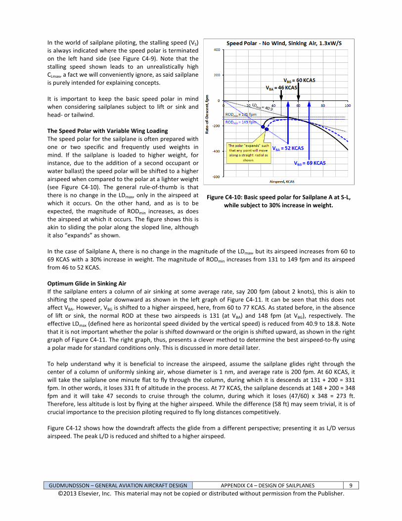
The Speed Polar with Variable Wing Loading

The speed polar for the sailplane is often prepared with

one or two specific and frequently used weights in

mind. If the sailplane is loaded to higher weight, for

instance, due to the addition of a second occupant or

water ballast) the speed polar will be shifted to a higher

airspeed when compared to the polar at a lighter weight

(see Figure C4-10). The general rule-of-thumb is that

there is no change in the LDmax, only in the airspeed at

which it occurs. On the other hand, and as is to be

expected, the magnitude of RODmin increases, as does

the airspeed at which it occurs. The figure shows this is

akin to sliding the polar along the sloped line, although

it also “expands” as shown.

Figure C4-10: Basic speed polar for Sailplane A at S-L,

while subject to 30% increase in weight.

In the case of Sailplane A, there is no change in the magnitude of the LDmax, but its airspeed increases from 60 to

69 KCAS with a 30% increase in weight. The magnitude of RODmin increases from 131 to 149 fpm and its airspeed

from 46 to 52 KCAS.

Optimum Glide in Sinking Air

If the sailplane enters a column of air sinking at some average rate, say 200 fpm (about 2 knots), this is akin to

shifting the speed polar downward as shown in the left graph of Figure C4-11. It can be seen that this does not

affect VBA. However, VBG is shifted to a higher airspeed, here, from 60 to 77 KCAS. As stated before, in the absence

of lift or sink, the normal ROD at these two airspeeds is 131 (at VBA) and 148 fpm (at VBG), respectively. The

effective LDmax (defined here as horizontal speed divided by the vertical speed) is reduced from 40.9 to 18.8. Note

that it is not important whether the polar is shifted downward or the origin is shifted upward, as shown in the right

graph of Figure C4-11. The right graph, thus, presents a clever method to determine the best airspeed-to-fly using

a polar made for standard conditions only. This is discussed in more detail later.

To help understand why it is beneficial to increase the airspeed, assume the sailplane glides right through the

center of a column of uniformly sinking air, whose diameter is 1 nm, and average rate is 200 fpm. At 60 KCAS, it

will take the sailplane one minute flat to fly through the column, during which it is descends at 131 + 200 = 331

fpm. In other words, it loses 331 ft of altitude in the process. At 77 KCAS, the sailplane descends at 148 + 200 = 348

fpm and it will take 47 seconds to cruise through the column, during which it loses (47/60) x 348 = 273 ft.

Therefore, less altitude is lost by flying at the higher airspeed. While the difference (58 ft) may seem trivial, it is of

crucial importance to the precision piloting required to fly long distances competitively.

Figure C4-12 shows how the downdraft affects the glide from a different perspective; presenting it as L/D versus

airspeed. The peak L/D is reduced and shifted to a higher airspeed.



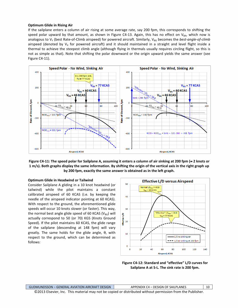
Optimum Glide in Rising Air

If the sailplane enters a column of air rising at some average rate, say 200 fpm, this corresponds to shifting the

speed polar upward by that amount, as shown in Figure C4-13. Again, this has no effect on VBA, which now is

analogous to VY (best Rate-of-Climb airspeed) for powered aircraft. Similarly, VBG becomes the best-angle-of-climb

airspeed (denoted by VX for powered aircraft) and it should maintained in a straight and level flight inside a

thermal to achieve the steepest climb angle (although flying in thermals usually requires circling flight, so this is

not as simple as that). Note that shifting the polar downward or the origin upward yields the same answer (see

Figure C4-11).

Figure C4-11: The speed polar for Sailplane A, assuming it enters a column of air sinking at 200 fpm (≈≈≈≈ 2 knots or

1 m/s). Both graphs display the same information. By shifting the origin of the vertical axis in the right graph up

by 200 fpm, exactly the same answer is obtained as in the left graph.

Optimum Glide in Headwind or Tailwind

Consider Sailplane A gliding in a 10 knot headwind (or

tailwind) while the pilot maintains a constant

calibrated airspeed of 60 KCAS (i.e. by keeping the

needle of the airspeed indicator pointing at 60 KCAS).

With respect to the ground, the aforementioned glide

speeds will occur 10 knots slower (or faster). This way,

the normal best angle glide speed of 60 KCAS (VBG) will

actually correspond to 50 (or 70) KGS (Knots Ground

Speed). If the pilot maintains 60 KCAS, the glide range

of the sailplane (descending at 148 fpm) will vary

greatly. The same holds for the glide angle, θ, with

respect to the ground, which can be determined as

follows:

Figure C4-12: Standard and “effective” L/D curves for

Sailplane A at S-L. The sink rate is 200 fpm.



In a 10 knot tailwind: ( ) ( )[ ] °−=θ∆°=×=θ − 20.020.1688.17060/148tan 1

In no-wind conditions: ( ) ( )[ ] °=×=θ − 40.1688.16060/148tan 1

In a 10 knot headwind: ( ) ( )[ ] °+=θ∆°=×=θ − 27.067.1688.15060/148tan 1

Where ∆θ represents the difference between the still air and windy glide-angle condition. This is shown

schematically in Figure C4-14. If the sailplane begins its glide 1000 ft above the ground, it will touch down in

1000/148 = 6m45s in all three cases, however, the range in headwind will be approximately (50 nm/60 min) x (6.75

min) = 5.63 nm, 6.76 nm in still air, and 7.88 nm in tailwind.

Figure C4-13: The speed polar for Sailplane A, assuming it enters a lift of 200 fpm (≈≈≈≈ 2 knots or 1 m/s). Both

graphs display the same information. By shifting the origin of the vertical axis in the right graph down by 200

fpm, exactly the same answer is obtained as that in the left graph.

Figure C4-14: A simple schematic showing the impact of head- or tailwind on the glide range assuming the pilot

maintains the same indicated (or calibrated) airspeed in all three cases.

This begs the question: In headwind, is there an airspeed other than 60 KCAS that yields range greater than 5.63

nm? To answer this question, assume that this time Sailplane A is being flown in a 10 knot headwind at 63 KCAS.



The ROD at this airspeed is 156 fpm. The ground speed will be 53 KGS and the glide will last for 1000/156 = 6m24s

(approximately 6.40 min). In that time, it will cover (53 nm/60 min) x (6.40 min) = 5.65 nm, which is greater than

5.63 nm at 60 KCAS. This shows that increasing the airspeed (up to a certain point) in headwind, yields greater

range. The inverse is true for tailwind.

It should be clear that a sailplane gliding in headwind equal to its forward speed in magnitude will not make any

headway with respect to the ground. Rather it would descend vertically – its glide angle would be 90°. Horizontal

distance can only be achieved by a forward glide speed faster than the headwind. The airspeed that yields the

greatest range can be determined by shifting the origin of the speed polar horizontally by a distance that equals

the wind speed, and then draw a tangent to the speed polar. Like the previous discussion demonstrates, in

headwind, the origin of the coordinate system is shifted sideways to the right, while for tailwind it is shifted to the

left, as shown in Figure C4-15.

Figure C4-15: The speed polar for Sailplane A, for a glide in a 10 knot tail- and headwind. By shifting the origin of

the horizontal axis to the left or right by 10 knots, an ideal airspeed for glide is obtained.

Speed-to-Fly

The preceding discussion shows that a speed polar for no wind, no thermal conditions can be used with ease to

determine the proper airspeed to fly in any non-standard conditions in order to maximize the range of the

sailplane. The particular airspeed obtained this way is referred to as Speed-to-Fly by sailplane pilots. It is

determined by shifting the origin around as shown in Figure C4-17. For headwind, the origin is shifted to the right.

For headwind and sink, it is shifted to the right and up, and so on.

Average Cross-Country Speed

Physics dictates that while cruising toward a thermal a sailplane will exchange altitude for distance. Ideally, once

inside the thermal the altitude will eventually be recovered. The total time consumed to travel to the thermal and

“get back” to the original altitude is a figure of merit not just for sailplanes, but also piloting skills in long distance

competitions. Consider the sailplane depicted in Figure C4-16, where the segment A-B is the glide segment and B-C

the climb segment. The average cross-country speed, denoted by Vavg (also shown in Figure C4-17) can be defined

as the distance travelled to the thermal divided by the total time it takes to reach it and recover the lost altitude.

Mathematically, this can be represented as follows:



climbglide tt

R

t

RV

glideglide

avg+

== (C4-1)

Where tglide and tclimb is the time spent in the glide and climb phases, respectively, and Rglide is the total distance

covered. The three variables (Rglide, tglide, and tclimb) are further defined as follows:

Figure C4-16: Definition of a cross-country model. (Adapted from Reference 6)

CSS

GSglide

V

Ht

V

HtH

V

VR ==

= climbglide (C4-2)

Where: VS = Vertical speed in glide

VGS = Arbitrary horizontal (forward) glide speed (see Figure C4-16)

VC = Vertical speed in climb

Insert these into Equation (C4-1) and manipulate algebraically to yield:

SC

C

GS

avg

SC

CGSavg

VV

V

V

V

VV

VVV

+=⇒

+= (C4-3)

The speed of climb, VC, is the difference between the thermal strength (the rate at which air is rising), denoted by

VT, and the rate of sink of the sailplane as it circles inside the thermal, VSC:

SSCT

SCT

GS

avg

SCTCVVV

VV

V

VVVV

+−

−=⇒−= (C4-4)

Optimum Speed-to-Fly between Thermals in Still Air

The preceding discussion pertains to the optimization of distance flown in still or moving air. It does not answer

what optimum airspeed to maintain when flying between thermals and this must be answered for still or moving

air as well.



Figure C4-17: Putting it all together – here for Sailplane A. The appropriate directions in which to move the

origin of the polar based on wind and thermal properties are shown. Then, a tangent from the offset origin to

the polar is drawn to reveal the Speed-to-Fly and average cross-country speed.

Consider Sailplane A in Figure C4-18 at Point A, as it begins its 4 nm journey toward a thermal, some 2000 ft above

the ground. Further, assume the thermal strength is known to be 400 fpm. Say the pilot considers 3 airspeeds to

fly; V1 = VBG = 60 KCAS, V2 = 80 KCAS, and V3 = 100 KCAS. Each will lead to different results. Clearly, maintaining VBG



will lead to the longest travel time (since it is the slowest speed), however, it also leads to the least amount of

altitude to be made up. Conversely, maintaining V3 leads to the earliest arrival time, but the greatest altitude to be

made up. Details of this speed selection is shown in Table C4-2, which assumes uniform S-L atmospheric properties

and that VBA is maintained in the thermal in all three cases (in straight and level flight). It can be seen that the

second airspeed, V2 = 80 KCAS, is superior to the other two, as it leads to the least amount of total time required to

reach the original altitude of 2000 ft. Consequently, its Vavg is the fastest.

Figure C4-18: Sailplane A headed to a thermal whose strength is known to be 400 fpm.

Table C4-2: Summary of Trip Parameters for a 4 nm Cruise to a Thermal and Subsequent Climb to 2000 ft

In addition to the airspeed, V, Table C4-2 shows the lift-to-drag ratio, vertical speed, VS, in fpm, altitude lost en

route, ∆Hcruise, in ft, time in cruise, ∆tcruise, time to climb back to 2000 ft, ∆tclimb, and total time, ∆ttotal, all in minutes.

The last column is an indication of progress made during the glide and subsequent climb. It is the average cross-

country speed, here 4 nm divided by the total time, ∆ttotal.

Figure C4-19 shows how Vavg varies with Vspeed-to-fly for Sailplane A on an idealized no-wind day with a thermal of

strength 400 fpm. It is assumed that the pilot maintains VBA once entering the thermal and that the thermal is large

enough to allow shallow bank angle to be maintained. The right graph shows how the speed polar can be used to

extract Vspeed-to-fly, while allowing Vavg to be extracted at the same time. Shift the origin to 269 fpm, which is the

thermal strength (400 fpm) added to the ROD at VBA (-131 fpm) to read 82 and 43 KCAS to be read, respectively.

The mathematical derivation of why this leads to the correct result is beyond the scope of this text, but an

interested reader is directed to Reference 7.

Optimum Speed-to-Fly between Thermals in Moving Air

If the sailplane is subject to lift or sink, as well as head- or tailwind, the Vavg and Vspeed-to-fly can be determined by

moving the origin of the flight polar to a new position dictated by the wind and the expected climb rate in the

thermal as explained earlier and as shown in the right graph of Figure C4-19. This airspeed can also be determined

analytically using Equation (C4-3), which leads to the following solution that requires an iterative scheme to solve

for the optimum lift coefficient, CLopt, given some expected rate-of-climb, VC:



Optimum lift coefficient: 08

232

min =ρ

−− LoptCLoptD CW

SVkCC (C4-5)

With CLopt known, the average cross-country speed can be calculated from Equation (C4-6) below. Since the

expression is actually applicable to any lift coefficient, CL, this is used rather than CLopt to indicate this flexibility.

Average cross-country speed:

23

2

min

21

2 L

LDC

LCavg

C

kCC

W

SV

CVV

++

ρ=

−

(C4-6)

Figure C4-19: Left graph shows how Vavg varies with the Speed-to-Fly for Sailplane A under specific conditions.

The right graph shows how the speed polar can be used to extract Vspeed-to-fly and Vavg.

DERIVATION OF EQUATIONS (C4-5) AND (C4-6):

The glide speed for a glide angle close to zero is given by Equation (21-11). Using small angle relations this is:

S

W

CS

W

CV

LL

GSρ

≈ρ

θ=

2cos2

The rate of descent is give by Equation (21-12): S

W

C

CVV

L

DSV

ρ==

223

Replacing the corresponding terms in Equation (C4-3) leads to:



23

21

23

21

23

2123

23 22

2

2

2

2

L

DC

LC

L

DC

LC

DCL

LLC

L

DC

L

C

SC

CGSavg

C

C

W

SV

CV

C

C

S

W

V

CV

S

WCVC

S

WCCV

S

W

C

CV

S

W

CV

VV

VVV

+ρ

=

+

ρ

=

ρ+

ρ=

ρ+

ρ=

+=

−−

−

If the drag is represented using the simplified drag polar, CD = CDmin + k∙CL², this becomes:

21

23

min

21

23

2

min

21

22L

L

DC

LC

L

LDC

LCavg

kCC

C

W

SV

CV

C

kCC

W

SV

CVV

++ρ

=+

+ρ

=−−

(i)

This is Equation (C4-6). The optimum CL is obtained by differentiating Equation (i) with respect to CL and setting the

derivative to zero. Using the quotient rule of calculus (e.g. Section E.6.3, Derivatives of Simple Functions) where we

define the functions f and g and their derivatives as follows:

2125

min

21

23

min

2321

2

1

2

3

2

2

−−

−−

+−=⇒++ρ

=

−=⇒=

LLDL

L

DC

LCLC

kCCCdgkCC

C

W

SVg

CVdfCVf

Using this with the derivative of the function f/g (as stipulated by the quotient rule) we get:

( )0

2

2

1

2

3

222

21

23

min

2125

min

2121

23

min

23

=

++

ρ

+−−

++

ρ

−

=

−−−−

L

L

DC

LLDLCL

L

DC

LC

L

avg

kCC

C

W

SV

kCCCCVkCC

C

W

SV

CV

dC

dV

Or more conveniently:

( ) 02

1

2

3

22

2125

min

2121

23

min

23

=

+−−

++

ρ

− −−−

−

LLDLCL

L

DC

LC kCCCCVkCC

C

W

SV

CV

Some algebraic acrobatics of this equation leads to Equation (C4-5).

QED

The MacCready Speed Ring

Being able to accurately maintain the proper airspeed in a sailplane is vital for anyone striving to maximize the

range. A selection of the optimized airspeed requires constant pilot awareness of the lift, sink, and wind speed in

the immediate surroundings. For this reason, while flying long distances, the sailplane pilot may frequently adjust

the airspeed to the variability of the atmosphere. To help, a special device called the MacCready ring is mounted

to the variometer (the Rate-of-Climb indicator) in the sailplane. Essentially, the device is a dial or a ring, on which

airspeeds for various sink or lift conditions are marked. The ring is rotated such that its index arrow indicates the

lift expected in the next thermal. This rotates the airspeed markings such the needle of the variometer points at

Vspeed-to-fly, allowing the pilot to quickly read this airspeed without having to resort to the speed polar. The name of



the device is attributed to the late Dr. Paul MacCready (1925-2007) who developed it. More details on the

operation of this device is beyond the scope of this text, but interested reader is pointed to any of the cited

references and many other sources available and intended for sailplane pilots. Today, sailplanes use electronic

variometers and flight computers that provide this information in real time.

Circling Flight

Once in a thermal, standard procedures call for the pilot to fly the sailplane in circles to take advantage of the

rising air. Unfortunately, as the sailplane banks its sink rate (VSC) increases over its value in straight and level flight

(VS). The steeper the bank, the greater is the sink rate and less potential energy is gained per unit time. The

advantage of a steep bank is smaller turning radius, which allows the pilot to better maneuver inside the thermal

and stay closer to its core region where lift is the greatest. This implies that an optimum bank angle exists that

maximizes the rate of climb, given a specific turning radius and strength of lift.

Before determining this optimum bank angle, we must develop formulation that allows the sink rate to be

assessed based on bank angle and turning radius. For this, consider Figure C4-20, which shows the forces acting on

the sailplane banking at an angle φ, while flying at airspeed V. L is the lift, W the weight, m the mass, and R is the

turn radius. If these are known, the sinking speed in circling flight can be determined from:

43

223

121

12

⋅⋅

ρ−

ρ=

L

L

D

SC

CgRS

WS

W

C

CV

(C4-7)

Figure C4-20: Forces acting on the sailplane as it is banked in a circling flight.

Using Equation (C4-7) the map shown in Figure C4-21 can be utilized to evaluate the turning performance of the

sailplane, which is imperative for circling flight inside thermals. The diagram shows that if a given bank angle is

maintained, the turn radius reduces only if the sailplane slows down. Similarly, for a fixed airspeed, the turn radius

can only be reduced by banking steeper – which increases the sink rate further. It also shows that, for instance, for

a 60° bank angle, the least sink rate is to be had around 67 KCAS, resulting in a turning radius of about 225 ft. Both

styles of curves are plotted using Equation (C4-7). The solid curves are generated by first calculating CL for a range

of airspeeds using Equation (19-42) assuming a fixed φ. The CLs are then used to calculate CD using the drag polar.

The turning radius is also computed using Equation (iii) in the following derivation. Finally, these are inserted into



Equation (C4-7). The dashed curves are calculated for a range of turning radii and fixed airspeeds. First, the bank

angle is calculated using Equation (i) in the derivation below. Then, this is used to calculate CL and CD as before.

Again, these are inserted into Equation (C4-7).

Note that Equation (C4-7) can be used during the design stage to help shape parameters, such as wing area, AR,

and drag characteristics, in an attempt to contour the turn performance curves towards a desirable turn radius and

bank angle inside a thermal of specific characteristics. Of course, this must take into account the net rate of climb,

VT + VSC, assuming VSC has a negative value. Recall that VT is the thermal strength (e.g. in ft/s or m/s) and VSC is the

rate of sink of the sailplane as it circles inside the thermal. A proper determination requires thermals to be

modeled mathematically, as presented below.

Figure C4-21: Turn performance map for Sailplane A, shows its rate-of-descent while banking at the specific

angles and airspeeds.

DERIVATION OF EQUATION (C4-7):

The freebody diagram of Figure C4-20 shows that: Rg

V

mg

RmV 22

tan ==φ (i)

Therefore: φ= tanRgV (ii)

or φ

=tan

2

g

VR (iii)

Using these equations, any of the variables V, φ, and R, can be estimated if two of the others are known. Then,

Equation (19-42), repeated here for convenience, can be used to estimate the speed of the airplane as a function

of the lift coefficient, CL, and bank angle, φ:



φρ=

cos

12

LSC

WV (19-42)

More conveniently, the equation can be used to extract the lift coefficient, CL, required during bank at a given

airspeed, from which the drag coefficient, CD, can be determined. Using Equation (ii) a relationship between the

airspeed, bank angle, and turning radius can be established:

φ

φ=φ=

φρ=

cos

sintan

cos

122 RgRgSC

WV

L

Which leads to: RgSC

W

Lρ=φ

2sin

Using the trigonometric identity cos² x + sin² x = 1, it is now possible to write:

2

21cos

ρ−=φ

RgSC

W

L

This relates the turning radius to the bank angle. Inserting this into Equation (21-13) yields Equation (C4-7).

QED

EXAMPLE C4-1:

Estimate the sink rate for Sailplane A as it banks 45° at an airspeed of 90 KCAS. Its wing loading is W/S = 10 lbf/ft².

Use the drag model given earlier, CD = 0.010 + 0.01498∙CL² and assume S-L conditions.

SOLUTION:

First estimate the lift coefficient at the condition using Equation (19-42):

( )( )( ) 5154.0

45cos

110

688.190002378.0

2

cos

1222

=

°×=

φ

ρ=

S

W

VCL

This contrasts 0.3644 for the straight and level condition at the same airspeed. Next calculate the drag coefficient:

( ) 01398.05154.001498.0010.001498.0010.022 =+=+= LD CC

Calculate the turn radius: ( )

( )ft711

45tan174.32

688.190

tan

22

=×

=φ

=g

VR

Then insert values into Equation (C4-7) to get the ROD in ft/s:



( )( )

( )

ft/s906.5

5154.0174.32711

110

002378.0

21

110

002378.0

2

5154.0

01398.0

121

12

432

23

432

23

=

××−

=

⋅⋅

ρ−

ρ=

L

L

D

SC

CgRS

WS

W

C

CV

Thermal Velocity Profiles

The 3-dimensional shape of thermals is of vital

importance to the design and operation of sailplanes.

Since thermals are of finite dimension, the sailplane

pilot must assertively bank inside it and ideally circle

around its core while gaining as much altitude as

possible. A small turning radius allows the maximum

lift to be extracted out of the thermal. However, the

smaller the turning radius the steeper is the bank

required. This inevitably comes at the cost of reduced

climb rate. Too shallow a bank will fly the sailplane out

of the thermal. Too steep a bank will reduce the

altitude gain and may even result in altitude being lost.

Being able to mathematically describe the vertical

velocity inside the thermal is thus fundamental to

determine the optimum bank angle, given the distance

of the sailplane from the core.

Figure C4-22: Common models used to approximate the

vertical speed profile inside a thermal. r/R = 0

Reference 2 presents a number of thermal profiles, of which three are shown in Figure C4-22. Generally, the

vertical speed in a thermal, denoted by VT, will be greatest at its core. This maximum speed is denoted by VT0. Even

though the following mathematical models indicate the thermal is symmetrical, this is not necessarily so in real

thermals. The three thermal profiles are defined mathematically below. The ratio r/R denotes the fractional

distance from the center of a thermal whose diameter is 2R. Of the three presented, the Power-Law, using n = 2 is

sometimes used for competition handicapping purposes2, assuming a thermal radius of R = 1000 ft and with a core

strength VT0 = 4.2 knots.

Power-Law Velocity Profile: ( )n

T

T RrV

V−=1

0

(C4-8)

Spherical Bubble Model: ( )

( )[ ] 5.22

2

0 21

1

Rr

Rr

V

V

T

T

−

−= (C4-9)

Modified Parabolic Model: ( )[ ] ( )22

0

1 Rr

T

T eRrV

V −⋅−= (C4-10)



The second element of thermal velocity profiles is their strength. Carmichael10

defines thermal strength in as

described below:

(1) Strong thermal has a maximum vertical speed of 20 ft/s (≈ 12 knots) that falls to 10 ft/s when r = 200 ft.

(2) Weak thermal has a maximum vertical speed of 10 ft/s (≈ 6 knots) that falls to 5 ft/s when r = 200 ft.

(3) Wide thermal has a maximum vertical speed of 15 ft/s (≈ 9 knots) that falls to 7.5 ft/s when r = 400 ft.

This information can be combined with the turn performance map to create a representation displaying the

optimum bank angle given specific airspeed. This is shown for Sailplane A in Figure C4-23. The optimum climb for

the selected airspeeds is easily identifiable. The map also shows that only airspeeds below 80 KCAS will result in

climb in this condition and that exceeding 30° of bank is detrimental to the climb performance.

Figure C4-23: Turn performance map for Sailplane A assuming a maximum thermal radius of 1000 ft and core

strength of 4.2 knots used to evaluate best ROC and the corresponding speed and bank angle.

The thick dashed, blue-colored curves in Figure C4-23 are obtained by adding VT to the VSC, which is calculated

using Equation (C4-7). The value of VT is calculated using any of the Equations (C4-8) through (C4-10). Effectively

this shifts the fixed VSC -isobars (the thin dashed gray-colored curves) upward into the new position, with the

associated maximums.



C4.1.3 Constraint Diagram for a Sailplane

In addition to the preceding turn performance map, a constraint diagram can also be developed to learn more

about design limitations. Constraint diagrams for powered aircraft are presented in Section 3.2, Constraint

Analysis. The absence of power for sailplanes and gliders means that constraints other than T/W must be

considered. The most obvious performance parameter is the Lift-to-Drag ratio (L/D). Just like the designer had to

“presume” a likely minimum drag coefficient, CDmin, and Aspect Ratio, AR, this is also required for sailplanes. Then,

for a given CDmin and AR, the question might be: Assuming the planform design will be such that an Oswald’s

efficiency of a given value, say 0.9, will be achieved, what wing loading, W/S, and LDmax yield desired airspeeds of

the minimum sink, VBA, or minimum angle (best glide), VBG?

For instance, consider a scenario in which we are convinced our sailplane will achieve a CDmin = 0.008 and e = 0.95.

It is of interest to determine the combinations of W/S and LDmax that renders VBA = 45 KCAS and VBG = 55 KCAS. This

is what a sailplane constraint diagram can reveal. The development of such a diagram requires selected glide

performance equations to be transformed into LDmax that is a function of W/S. Note that all the following

expressions assume the simplified drag model. This is justified on the basis that the constraint diagram will get us a

“ballpark” value.

LDmax for a Desired VBA

The following expression is used to determine the combinations of W/S and LDmax required to achieve a desired

airspeed of minimum sink rate at a given altitude. The airspeed must be true airspeed. The first step in its

application is to convert the airspeed into dynamic pressure, qBA. Then the constraint can be calculated using the

following expression:

22

min

max

1

+

=

S

W

q

kkC

LD

BA

D

(C4-11)

LDmax for a Desired VBG

The following expression is used to determine the combinations of W/S and LDmax required to achieve a desired

airspeed of minimum glide angle at a given altitude. The airspeed must be true airspeed. The first step in its

application is to convert the airspeed into dynamic pressure, qBG. Then the constraint can be calculated using the

following expression:

22

min

max

3

1

+

=

S

W

q

kkC

LD

BG

D

(C4-12)

An example of the application of these formulas is shown in Figure C4-24. To read the graph, consider a sailplane

slated to have an AR of 28 with an expected CDmin = 0.008 and e = 0.95, and for which a desired VBA > 45 KCAS and

VBG > 55 KTAS. This is possible as long as its W/S is greater than 10.5 lbf/ft² and LDmax exceeds 48. For comparison,

Reference 11 shows the Stemme S10 (for which this sample is intended to resemble) has a LDmax of 51, VBA ≈ 45

KCAS, and VBG ≈ 55 KCAS, at a W/S = 9.3 lbf/ft², showing that this method is not far off the mark.

It should be stressed that a constraint diagram of this nature is not sufficient to design a sailplane. An optimization

that takes into account it glide characteristics in thermals, as presented in the preceding section, is also called for.



Figure C4-24: A constraint diagram for a hypothetical sailplane, whose CDmin and Oswald’s efficiency factor are

expected to be 0.010 and 0.9, respectively.


Begin with Equation (19-18) and rearrange as follows:

2

max

min

min

max

14

4

1

LDkC

kCLD D

D

=⋅⋅⇒

⋅⋅= (i)

Then, consider the expression for the airspeed of minimum sink rate, VBA, given by Equation (21-14). Multiply the

term under the second radical by k/k. Then, separate the altitude and W/S terms from the radical as follows:

41

min

2

min

2

min 3

2

3

2

3

2

ρ=

ρ=

ρ=

kC

k

S

W

kC

k

S

W

C

k

S

WV

DDD

BA

Then, add and subtract CDmin∙k from the denominator of the quartic:

41

minmin

241

min

2

4

2

3

2

−

ρ=

ρ=

kCkC

k

S

W

kC

k

S

WV

DDD

BA

The positive term in the denominator of the quartic is the square of the LDmax. Insert to get:



41

min

2

max

2

1

2

−

ρ=

kCLD

k

S

WV

D

BA

Square both sides and note that 2

21

BGBG Vq ρ=

( ) kCLD

k

SW

q

kCLD

k

S

WV

D

BA

D

BA

min

2

max

22

min

2

max

22

11

2

−=

⇔

−

ρ=

Then, solve for LDmax:

22

min

max

22

2

2

2

min

2

max

11

+

=⇔

=

=−

S

W

q

kkC

LDS

W

q

k

q

S

Wk

kCLD

BA

D

BABA

D

QED


Proceed in a similar fashion as above using the expression for the airspeed of minimum glide angle, VBG, given by

Equation (21-16). Multiply the term under the second radical by k/k. Then, separate the altitude and W/S terms

from the radical as follows:

41

min

2

min

2

min

222

ρ=

ρ=

ρ=

kC

k

S

W

kC

k

S

W

C

k

S

WV

DDD

BG

Then, add and subtract 3CDmin∙k from the denominator of the quartic:

41

minmin

241

minminmin

2

34

2

33

2

−

ρ=

−+

ρ=

kCkC

k

S

W

kCkCkC

k

S

WV

DDDDD

BA

The positive term in the denominator of the quartic is the square of the LDmax. Insert to get:

41

min

2

max

2

31

2

−

ρ=

kCLD

k

S

WV

D

BA

Square both sides and note that 2

21

BABA Vq ρ=

( ) kCLD

k

SW

q

kCLD

k

S

WV

D

BA

D

BA

min

2

max

22

min

2

max

22

3131

2

−=

⇔

−

ρ=

Then, solve for LDmax:



22

min

max

22

2

2

2

min

2

max

3

131

+

=⇔

=

=−

S

W

q

kkC

LDS

W

q

k

q

S

Wk

kCLD

BA

D

BABA

D

QED

C4.1.4 Sailplane Tail Design

Designing the empennage for a sailplane is identical to that of powered airplanes, minus the thrust contribution,

unless of course, the sailplane is powered. The tail should be sized such that handling and controllability complies

with the applicable paragraphs of CS-22 (EASA Certification Specifications for Sailplanes and Powered Sailplanes).

In particular, this involves Subpart B, Flight, paragraphs 22.21 through 22.255.

Just like the conceptual design of powered aircraft, the first estimation can be made using the conventional

historical tail volume methods of Section 11.5, Initial Tail Sizing Methods. This will get the tail size in the “ballpark.”

The next step is to evaluate if the resulting geometry provides the necessary elevator or rudder authority during

some extreme conditions stipulated in Subpart B. For a sailplane, cross-wind landing, stalling and flaps down at low

airspeeds with a forward CG position, and possibly aerotow or winch operations during T-O would present a

challenge. There is no balked landing case to contend with, unless the sailplane is powered.

Requirements for Elevator Deflection to Trim

Equation (11-25) can be used to estimate the AOA and elevator deflection to trim at various conditions. The

expression is presented in its simplified form below, by setting all thrust terms to 0:

δ−−

δ−−

δ−−

=

δ

α

δ

δ

δ

δα

δα

δα

fmm

fLL

fDD

e

mm

LL

DD

f

f

f

e

e

e

CC

CCqS

W

CC

CC

CC

CC

0

0

min

(C4-13)

The terms are detailed in Chapter 11, The Anatomy of the Tail. The formulation allows the effect of flaps as means

to lower stalling speed or as cruise flaps to be included. The expression should be used to estimate if excessive

elevator deflection is required for the maneuvers stipulated in CS-22. If so, the elevator and the HT geometry must

be resized.

Stick-Fixed Neutral Point

Equation (11-26), reproduced below for convenience, can be used to estimate the location of the stick fixed

neutral point:

α

αα

α

α−

⋅π−⋅⋅+=

L

mL

L

L

HT

MGC

AC

MGC

n

C

C

AR

C

C

CV

C

h

C

hACHT

21 (11-26)

Again, see Chapter 11 for the definition of terms. Note that it is assumed that the tail efficiency for a sailplane is

1≈ηHT , so it is omitted from the equation. Since the horizontal tail volume is defined as

MGC

HTHTHT

CS

lSV

⋅

⋅= , the

expression can be used to estimate the product HTHT lS ⋅ for a given wing geometry and expected (or desired)

Static Margin (SM), defined as follows:



( ) MGCn ChhSM −= (C4-14)

Where h and hn are the physical location of the CG and stick-fixed neutral point measured from the LE of the CMGC.

Note that a 10% SM would be represented as 0.1 and so on. Introducing this to Equation (11-26) and assuming a

typical value of 25.0≈MGCAC Ch leads to:

( )

α

αα

α

α−

⋅π−⋅⋅+−=

−=

L

mL

L

L

HT

MGCMGC

n

C

C

AR

C

C

CV

C

h

C

hhSM ACHT

2125.0 (11-15)

This can be solved for the required horizontal tail volume as shown below:

( )αα

α

α

α

−⋅π

⋅π

++−=

LL

L

L

m

MGC

HTCAR

AR

C

C

C

C

C

hSMV

HT

AC

225.0 (11-16)

Once a suitable VHT has been determined, it is possible to optimize the tail arm length with respect to drag by

minimizing the wetted area. Such an optimization is identical to Methods 1 through 3 of Section 11.5, except that

the contraction of complex geometry may call for a numerical scheme to be implemented, rather than a closed

form analytical solution. In order to demonstrate how such optimization can be accomplished, a simplified

approximation of the tadpole configuration is represented below using two frustums.

Initial Tail Sizing Optimization using an Arbitrary Fuselage

Figure 12-3 shows a textbook tadpole fuselage from the side. While the contraction of the fuselage for real

applications is carefully crafted, a simplification like the one shown in Figure 12-25 can be utilized to demonstrate

the determination a tail arm length for a tadpole fuselage. The approach minimizes the combined wetted area of

the HT, VT, and tailboom, thus, minimizing skin friction drag. For convenience, the figure is reproduced below as

Figure C4-25, with the addition of a wing and HT, to better clarify the assumptions to be made. It must be stressed

that this method is only a geometric optimization. It does not guarantee that flow separation will not happen. If

the contraction of the aft fuselage is too rapid, the flow will separate, increasing the drag. The final shape will have

to be refined using a more sophisticated CFD analysis or wind tunnel testing to confirm that flow separation does

not occur.

For this optimization, it will be assumed that the forward part of the fuselage is only shaped to sustain NLF as far

back as possible. Typically, the NLF transitions into turbulent boundary layer near the LE of the wing. For this

reason, the forward part of the fuselage is assumed to not influence the required tail arm length. Therefore, it is

simply omitted from further consideration. The part of the fuselage of importance in the development of this

method extends approximately from the wing’s quarter chord to that of the HT, as shown in Figure C4-25. This

leaves us with the following control variables: L3, L4, D, d1, and d2. Furthermore, it will take into account a desired

VHT and VVT, identical to the approach of Section 11.5.3, METHOD 3: Initial Tail Sizing Optimization Considering

Horizontal and Vertical Tail.

Using these variables, the following formulas can be used to estimate the wetted area of the tail boom, but these

are taken directly from the approach of Section 12.4.4, Surface Areas and Volumes of a Tadpole Fuselage by using

Equation (12-10). Note that for convenience, the diameter variables will be related to the maximum fuselage

diameter, D, as follows:

sDdandrDd == 21

Additionally, let’s define the constant k: TlLk 3=



Figure C4-25: An approximation of a tadpole fuselage using elementary solids. Only the section of the fuselage

between quarter chord of the wing and HT are considered.

This reduces the number of variables from five to two. We can now write:

Tail arm length: ( )HTHTHT lkLandklLLLl −==⇒+= 14343 (C4-17)

Wetted area of frustum �: ( ) ( )2

222

1 142

1r

Dlk

rDS HTF −+

+π= (C4-18)

Wetted area of frustum �: ( ) ( ) ( )22

222

24

12

srD

lksrD

S HTF −+−+π

= (C4-19)

The total wetted area of the aft fuselage is the sum of SF1 and SF2:

( ) ( ) ( ) ( ) ( )

−+−++−++

π= 22

2222

222

411

41

2sr

Dlksrr

Dlkr

DS HTHTF

(C4-20)

Also, it is of interest to compare the wetted area of the tadpole fuselage to that of a standard frustum shape,

FstdS . This is easily calculated using Equation (12-10), where D1 = D and D2 = d2 = sD in Figure C4-25. The resulting

expression is given by:



Standard frustum: ( ) ( )

−+

+π= 2

22 1

42

1s

Dl

sDS HTFstd (C4-21)

Numerical comparison using typical sailplane geometry reveals that the reduction in surface area of a tadpole is

easily in the 20-35% range. All of the above equations are simple to derive using Equation (12-10). Additional

equations required are Equations (11-57) and (11-58), which are needed to calculate the planform areas of the HT

and VT, from which an approximation to their corresponding wetted areas is generated. In other words, if VHT and

VVT have been established, it is possible to calculate a corresponding SHT and SVT, which are then converted into

wetted areas. In its simplest form, the wetted area for the HT is 2∙SHT, although multiplying this by a factor like 1.05

to account for airfoil curvature is a more reasonable approach. An example of their use for a geometric

optimization is given below.

EXAMPLE C4-2:

Consider the Stemme S-10 style geometry shown in Figure C4-26. Note that the dimensions given may not

necessarily match that of the Stemme, as the purpose here is only to see if the above optimization will yield a

similar tail arm. Judging from three-views of the aircraft that are in the public domain, its tail arm (lT) is about 16.7

ft. The wing area is 201.3 ft², wing span is 75.5 ft, AR is 28.3, and a representative Taper Ratio of about 0.3 is

assumed. This results in a CMGC of 2.924 ft. Further assume the fuselage can be approximated using the tadpole

diagram of Figure C4-25, has a contraction location of 0.25∙lT, a max diameter of 3.75 ft, r = 0.4, and s = 0.156.

Determine the tail arm length, lT, that yields the minimum combined wetted area of the HT, VT, and tailboom using

historical values of VHT = 0.5 and VVT = 0.2, from Table 11-4. Use a 1.05 wetted area booster for the HT and VT.

Figure C4-26: A Stemme S-10 style geometry.

SOLUTION:

The solution is best accomplished by calculating the wetted area for a number of possible tail arm lengths, ideally

using a spreadsheet. This has been done in the Table C4-3 below. In the table, lHT varies from 5 to 20 ft. The

columns containing SHT and SVT were calculated using Equations (11-57) and (11-58) with the cited tail volumes.

The wetted areas in the next two columns is calculated using SHT WET = 2∙SHT∙1.05 and SVT WET = 2∙SVT∙1.05,

respectively. The columns containing SF1 and SF2 were calculated using Equations (C4-18) and (C4-19). The column

labeled SWET is the total wetted area (the cost function). It is simply the sum SHT WET + SVT WET + SF1 + SF2. Finally, the

column labeled SFstd was calculated using Equation (C4-21) and the last column is the ratio of wetted areas of the

standard frustum to the tadpole tailboom. For instance, if lT = 20 ft, the wetted area of the standard frustum is

27.8% greater than that of the tadpole.



A very pronounced minimum can be seen in the accompanying graph. It was found to correspond to an lT of 16.0

ft, although a more accurate evaluation shows it is closer to 15.8 ft. However, a tail boom length ranging from 14

to 18 ft will result in near optimum wetted area, giving the designer some flexibility when sizing the tail. Both

values are not too far from the reference value of 16.7 ft of the actual Stemme S-10. Note that analysis of a three-

view of the sailplane shows it has a VHT ≈ 0.44 and VVT ≈ 0.018. Similarly, its SHT ≈ 15.5 ft² and SVT ≈ 15.1 ft².

Table C4-3: Results from Tail Arm Optimization

C4.1.5 Sailplane Design Tips

With the exception of the importance of glide performance, the design of sailplanes is not all that different from

powered airplanes. Requirements for structures (weight, strength, stiffness), fabrication (manufacturing cost,

maintenance cost, material selection, production methodologies), ergonomics (field-of-view, control system

methodologies, cockpit accommodation), and flying qualities (natural static and dynamic stability, stall

characteristics) are similar in many ways. Certification requirements have many similarities and differences.

Ground handling of sailplanes is different as many allow for quick assembly and disassembly. Also, take-off using

aero-tow or winches must be considered. The same holds for jettisonable water ballast, generally not used in

powered GA aircraft. The high glide ratio of sailplanes calls for speed brakes or spoilers to allow for a steeper

approach path on final.

The certification of sailplanes and powered sailplanes is generally done through EASA standard CS-22, EASA

Certification Specifications for Sailplanes and Powered Sailplanes. As stated in Table 1-1, 14 CFR 21.17(b) allows the

FAA to tailor the certification on a need-to-basis to sailplanes. Then, by referring to AC 21.17-2A, the FAA accepts

the former JAR-22 (now CS-22) as a certification basis.

In addition to the preceding discussion, the following tips should be considered by the designer of sailplanes.

1 To improve climb

performance

• Reduce wing loading for improved circling characteristics

• Increase AR

• Increase Reynolds number

• Reduce CDmin and CDmisc

• Use a wing planform that best achieves elliptical lift distribution

• Consider the use of winglets or polyhedral planform

2 Cross-country performance

• Increase wing loading for higher interthermal airspeeds

• Increase AR

• Increase Reynolds number

• Reduce CDmin and CDmisc

• Use a wing planform that best achieves elliptical lift distribution

• Consider the use of winglets or polyhedral planform



3 Surface qualities

• The surface quality of sailplanes must be very smooth to stabilize the NLF.

• Composites are currently the best material for high-quality sailplane construction

• Class A surface qualities, which means that surface curvature, slope and

alignment of surfaces should be continuous wherever possible.

4 Wing design

• Consider wing planform shapes that generate constant section lift coefficients

along the span (elliptical lift distribution)

• High aspect ratio, as long as its structural weight impact is light

• Consider cruise flaps

• Seal gaps not needed for aerodynamic purposes. A gap between aileron and wing

is generally detrimental. A gap between a slotted flap and wing is beneficial

• NLF airfoils

5 Fuselage design

• Tadpole fuselage geometry

• Smooth surface qualities with faired intersections between it and the lifting

surfaces

• Retractable landing gear

• One piece canopy with smooth

C4.1.6 Design of Unmanned Aerial Vehicles

Just like the design of sailplanes, the design of Unmanned Aerial Vehicles (UAV) is far more involved than appears

at first glance. This is primarily due to the use of an autopilot that often must be capable of autonomous take-off

and landing. What aerodynamic appearance concerns, the UAV can be designed just like any other airplane.

However, the absence of human operators often calls for geometry dictated more by utility than aerodynamics

and, often, this results in statically unstable aircraft.

Configuration B in Figure C4-2 is one practical solution of many for a simple powered airplane with good long-

range or long-endurance reconnaissance mission, designed by the author for a UAV project. It features a tailboom

intended to protect the propeller as it was expected to land on unimproved strips. The T-tail was selected to

ensure it resides in the propwash to improve responsiveness at the low airspeeds, which is where the vehicle was

designed to operate most of the time. It also protects the tail when landing, as it ensures the plane will come to

rest on its wing. The cranked wing planform features a straight leading edge, but forward swept quarter chord

naturally diminishes section lift coefficients at the tip to improve roll stability a stall. This is compounded by the

cranked dihedral and, thus, reduces the need for excessive washout. It also helps to protect the wingtip if the

airplane lands on unimproved strips with ground vegetation. The size of the HT depends on the high thrust line,

which is necessitated by adequate propeller clearance.

UAVs have become very practical for tasks that for the most part require monotonous flying. The advent of small

but sophisticated autopilots and electronic gyros is in the process of transforming this branch of aviation. Such

aircraft are primarily intended for surveillance and research flight. They are often equipped with cameras that are

capable of tracking landmarks and transmit a live signal that also allows them to be flown manually from great

distances. Generally, the airframe is regarded as a platform to carry electronic surveillance equipment. For this

reason, many UAVs do not take advantage of advanced aerodynamics and it can be argued that selecting a tried

configuration is beneficial to some unusual configurations. Therefore, any of the aforementioned configurations

will work and many of the arguments for or against are applicable to the UAVs and the one’s that involve the

human factor can be ignored.



REFERENCES

1 NASA CR-2315, Motorless Flight Research, Althaus, Dieter, 1972.

2 Welch, Ann, Lorne Welch, and Frank Irving, The Complete Soaring Pilot’s Handbook, David McKay Company, 1977.

3 Fédération Aéronautique Internationale, Record ID 14043. Website is www.fai.org.

4 Fédération Aéronautique Internationale, Record ID 8198.

5 Boermans, L. M. M., Research on sailplane aerodynamics at Delft University of Technology - Recent and Present

Developments, presented to Netherlands Association of Aeronautical Engineers (NVvL), 2006. 6 Thomas, Fred, Fundamentals of Sailplane Design, College Park Press, 1999.

7 Reichmann, Helmut, Cross-Country Soaring, 2

nd Ed., Soaring Society of America, 1993.

8 Stewart, Ken, The Soaring Pilot’s Manual, 2

nd Ed., Airlife Publishing, 2008.

9 Scull, Bill, Soaring Across Country, Pelham Books, 1979.

10 Carmichael, Bruce H., What Price Performance, Soaring Magazine, May-June, 1954.

11 Anonymous, Flight Manual Stemme S10-V, Stemme AG, 1994.

appendix c4: design of sailplanes - elsevier · the modern sailplane features a tadpole fuselage,...

Documents