appendix - blade element momentum theory
DESCRIPTION
AeronauticsTRANSCRIPT

Appendix A-Blade Element Momentum Theory 176
APPENDIX A
Appendix A-Blade Element
Momentum Theory

Appendix A-Blade Element Momentum Theory 177
A.1. Introduction
With the availability of large computing power and developments in grid generation and
numerical algorithms, it is very tempting to compute the turbulent flow around a rotating
blade using the equations of motion in their differential forms, (Reynolds-averaged Navier-
Stokes equations). These equations need a model of turbulence to make them a closed set.
A large number of models of turbulence have been proposed, for example, mixing length
models, one-equation models, two-equation models, Reynolds stress models, algebraic
stress models, etc. Tulapurkara (1996) gives a review of these models in computation of
flow past aerofoils and wings.
A rotating blade is experiencing a wide range of angle of attacks along its span, from
negative values to post-stall values. A high angle of attack causes a strong adverse-
pressure-gradient separating flow in which no turbulent model can be applied accurately.
Applying the equations of motion in their integral forms (linear and angular momentum)
around the wind turbine (rather than the blade) together with the experimental data of blade
aerodynamic characteristics is an alternative to solve the flow field and find the blade
loading. This method is known as Blade Element Momentum Theory, BEMT.
A.2. Induced, total and relative velocity fields
Extracting energy from wind slow downs the wind speed and rotation of blades induces
some circumferential and radial velocities to the wind. Wind speed retardation depends on
the amount of the extracted energy (wind turbine loading), while the induced
circumferential velocity depends on the wind turbine angular velocity. Induced radial
velocity due to centrifugal forces is much smaller than the two other components and is
usually neglected.
Flow in the plane of a wind turbine rotor, from now on referred as disk, can be considered
as a combination of upstream mean velocity field, wV and induced velocity field, iV .
iw VVV += (A.1)
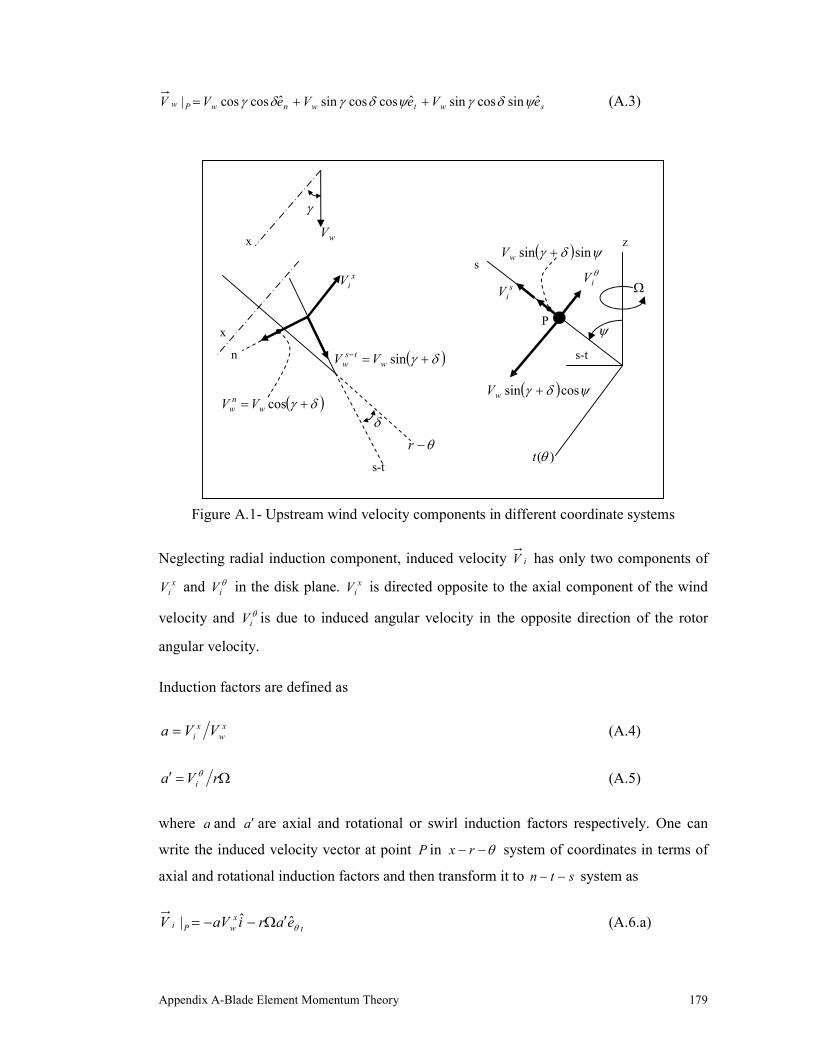
Figure (A.1) shows the coordinate systems used to represent velocity fields. In this figure:

Appendix A-Blade Element Momentum Theory 178
θ−− rx : Disk (rotor) system of coordinates
x : Rotor axis
θ−r : Rotor plane
r : Disk radial coordinate, 0<r≤ R; R: rotor radius
stn −− : Blade system of coordinates
n : Normal to the blade
st − : Blade plane
tn − : Aerofoil plane
s : Blade span-wise coordinates
γ : Yaw angle
δ : Conning angle
ψ : Azimuth angle
Ω : Rotor angular velocity
Here it is assumed that wind velocity has no vertical components ( 0=ZwV ).
Using the stn −− system of coordinates, wind velocity wV at a general point P can be
expressed as
( ) ( ) ( ) swtwnwPw eVeVeVV ˆsinsinˆcossinˆcos| ψδγψδγδγ +++++= (A.2)
Conning angle δ is usually very small and therefore δδ cossin << , but yaw angle γ can be
large enough such that γsin and γcos have the same order of magnitude. Neglecting terms
including δsin in comparison with the terms including δcos , Equation (A.2) can be
rewritten in a simpler form as
Appendix A-Blade Element Momentum Theory 179
swtwnwPw eVeVeVV ˆsincossinˆcoscossinˆcoscos| ψδγψδγδγ ++= (A.3)
Figure A.1- Upstream wind velocity components in different coordinate systems
Neglecting radial induction component, induced velocity iV has only two components of
xiV and θ
iV in the disk plane. xiV is directed opposite to the axial component of the wind
velocity and θiV is due to induced angular velocity in the opposite direction of the rotor
angular velocity.
Induction factors are defined as
x
w
x
i VVa = (A.4)
Ω=′ rVa i
θ (A.5)
where a and a′ are axial and rotational or swirl induction factors respectively. One can
write the induced velocity vector at point P in θ−− rx system of coordinates in terms of
axial and rotational induction factors and then transform it to stn −− system as
t
x
wPi eariaVV θˆˆ| ′Ω−−= (A.6.a)
s-t
γ
x
wV
xiV
( )δγ +=− sinwts
w VV
θ−r
( )δγ += coswnw VV
δ
n
θiV
( ) ψδγ sinsin +wV z
P
s-t
s
ψ
)(θt
siV
( ) ψδγ cossin +wV
Ω
x

Appendix A-Blade Element Momentum Theory 180
tnwPi eareaVV ˆˆcoscos| ′Ω−−= δγ (A.6.b)
Finally substituting wV from Equation (A.3) and iV from Equation (A.6.b) back into
Equation (A.1), velocity field in the plane of blade can be written as
swtwnw eVearVeaVV ˆsincossinˆcoscossinˆ)1(coscos ψδγψδγδγ +′Ω−+−=
(A.7)
For a moving blade the relative velocity of the flow at a point P located on the blade is
PbladePflowPrel VVV ||| −= (A.8)
where
tPblade erV ˆ| Ω= (A.9)
Combining Equations (A.7),(A.8) and (A.9) leads to
nwrel eaVV ˆ)1(coscos −= δγ
tw earV ˆ)1(coscossin ′+Ω−+ ψδγ
sw eV ˆsincossin ψδγ+ (A.10)
Figure (A.2) shows the relative velocity in the plane of blade aerofoil. Inflow angle and
normalised in-plane relative velocity can be derived from Figure (A.2) as
ψδγλδγ
ϕcoscossin)1(
)1(coscostan
−′+−
=a
a
r
(A.11)
and
ϕδγ
sin
)1(coscos| a
V
V
w
tnrel −=− (A.12)
where local velocity ratio, rλ is defined as

Appendix A-Blade Element Momentum Theory 181
w
rV
rΩ=λ (A.13.a)
or in terms of blade span coordinate s (δcos
rs = ):
w
rV
s Ω=
δλ
cos (A.13.b)
Figure A.2- Relative velocity in aerofoil plane
A.2.1. Special case – Zero yaw
In the case of zero yaw angle, 0=γ , Equations (A.4), (A.10), (A.11) and (A.12) can be re-
written as
w
x
i VVa = (A.14)
tnwrel eareaVV ˆ)1(ˆ)1(cos ′+Ω−−= δ (A.15)
)1(
)1(costan
a
a
r′+
−=
λδ
ϕ (A.16)
ϕδsin
)1(cos| a
V
V
w
tnrel −=− (A.17)
and the velocity diagram changes to Figure (A.3).
n
t
tnrelV −| ϕ
)1(coscos aVw −δγ
ψδγ coscossin)1( wVar −′+Ω
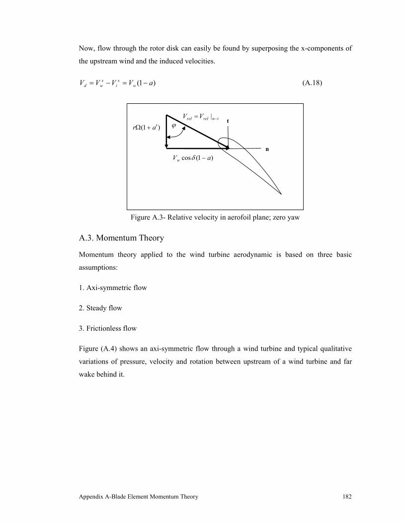
Appendix A-Blade Element Momentum Theory 182
Now, flow through the rotor disk can easily be found by superposing the x-components of
the upstream wind and the induced velocities.
)1( aVVVV w
x
i
x
wd −=−= (A.18)
Figure A.3- Relative velocity in aerofoil plane; zero yaw
A.3. Momentum Theory
Momentum theory applied to the wind turbine aerodynamic is based on three basic
assumptions:
1. Axi-symmetric flow
2. Steady flow
3. Frictionless flow
Figure (A.4) shows an axi-symmetric flow through a wind turbine and typical qualitative
variations of pressure, velocity and rotation between upstream of a wind turbine and far
wake behind it.
n
t ϕ
)1(cos aVw −δ
)1( ar ′+Ω
tnrelrel VV −= |

Appendix A-Blade Element Momentum Theory 183
Figure A.4- Pressure, velocity and rotation distributions
A.3.1. Thrust and torque coefficients
Applying the x-component of linear momentum equation to the annulus control volume
shown in Figure (A.5), gives thrust force as )( FWrotor VVdQdT −= ∞ρ ,where the volume
flow rate diskd dAVdQ = , wVV =∞ and )1( aVV wd −= and therefore
diskFWwwrotor dAVVaVdT ))(1( −−= ρ (A.19)
Applying the energy equation for the same control volume gives the turbine power.
)(5.0 22
FWwdiskd VVdAVdP −= ρ (A.20)
∞ Disk Far Wake
Pressure, P
Velocity, V
Rotation, ω

Appendix A-Blade Element Momentum Theory 184
Figure A.5- Annulus control volume; Linear momentum balance
Turbine power can also be obtained by multiplying the thrust force and flow velocity at the
disk.
ddTVdP = (A.21)
Combining Equations (A.19), (A.20) and (A.21) concludes
wFW VaV )21( −= (A.22)
By substituting FWV back in Equation (A.19), rotordT will be determined in terms of the
wind velocity at the upstream and the axial induction factor.
diskwrotor dAVaadT 2)1(2 ρ−= (A.23)
Thrust coefficient by definition is
diskw
TdAV
dTC
2
21 ρ
= (A.24)
And therefore as a result of Momentum Theory it becomes:
)1(4 aaCT −= (A.25)
CV
FWdQVρ dT ∞dQVρ

Appendix A-Blade Element Momentum Theory 185
To determine torque coefficient by the Momentum Theory one can start from applying the
angular momentum equation about the x-axis for the control volume shown in Figure (A.6)
to find a relation between the rotation in far wake and circumferential velocity at disk as
( ) ( ) ( ) θωωω diskdiskdiskFW rVrrrr 22/222 === .
Since the circumferential velocity θdiskV is only due to induction, one can substitute θθ
iVV =
from Equation (A.5) in the above equation to find ( )FWr ω2 .
( ) Ω′= arr FW
22 2ω (A.26)
Figure A.6- Annulus control volume; Angular momentum balance between disk and Far
Wake
Applying angular momentum equation about x–axis for the control volume shown in
Figure (A.7), the applied torque on the rotor will be determined.
( ) ( ) ∞−= ωωρ 22 rrdQdM FWx (A.27)
Combining Equations (A.26) and (A.27) gives the rotor torque as
diskwx dAraaVdM 2)1(2 ′−Ω= ρ (A.28)
Torque coefficient is defined as
CV
FWrdQ )( 2ωρ diskrdQ )( 2ωρ

Appendix A-Blade Element Momentum Theory 186
diskw
x
M
rdAV
dMC
2
21 ρ
= , (A.29)
and finally as a result of the Momentum Theory it becomes
)1(4 aaC rM −′= λ (A.30)
Figure A.7- Annulus control volume; Angular momentum balance
A.3.2. Tip and Hub Losses
In momentum theory, the axi-symmetric flow is the basic assumption, which holds if the
turbine rotor has an infinite number of blades with zero chord length. In the case of a real
turbine with a finite number of blades, the induced velocity on the blades is different from
the mean induced velocity in the flow annulus and therefore circumferential symmetry
does not hold. The non-uniformity of the induced flow field makes the actual local TC and
MC to be smaller than the expected values by the optimum actuator disk theory. The
departure of the induced velocity, TC and MC from their momentum theory values is more
significant near the tip and root of the blade. These deviations from the uniform induced
velocity flow field are called tip and hub losses. The overall loss factor, F is defined as
hubtipFFF = (A.31)
CV
FWrdQ )( 2ωρ
dM
∞)( 2ωρ rdQ

Appendix A-Blade Element Momentum Theory 187
In which tipF is unity at inboard parts of the blade and takes smaller values near the tip of
the blade and hubF is unity at outboard parts of the blade and takes smaller values near the
hub of the blade. Overall loss factor F can be applied on the induced velocity or disk
velocity.
A.3.3. Loss Models
Depending on which parameter or parameters are affected by F , different models will be
introduced. Most of commercial codes use two models that are known as
1. Classical or Wilson
2. Standard or Advanced or Wilson-Walker.
a. Classical Model
In Classical model, loss factor F is applied to the axial induced velocity:
w
x
i aFVV = (A.32)
and therefore
)1( aFVV wd −= (A.33)
)21( aFVV wFW −= (A.34)
)1(4 aFFaCT −= (A.35)
)1(4 aFaC rM −′= λ (A.36)
According to Figure (A.8), which shows the relative velocity diagram for this model, the
normalised relative velocity is given by Equation (A.37).
ϕδ
sin
cos)1(| aF
V
V
w
tnrel −=− (A.37)
b. Wilson-Walker Model

Appendix A-Blade Element Momentum Theory 188
In Wilson-Walker model, loss factor F is directly applied to the disk
velocity, )1( aFVV wd −= and the difference between the free stream velocity and far wake
velocity is defined as wFWw aVVV 2=− . With the above assumptions thrust and torque
coefficients can be calculated as:
)1(4 aFaCT −= (A.38)
)1(4 aFaC rM −′= λ (A.39)
For this model the relative velocity diagram becomes as shown in Figure (A.9) and the
normalised relative velocity becomes as given by Equation (A.40).
ϕδ
sin
cos)1(| Fa
V
V
w
tnrel −=− (A.40)
Figure A.8- Relative velocity in aerofoil plane; zero yaw; Classical model
Figure A.9- Relative velocity in aerofoil plane; zero yaw; Wilson-Walker model
n
t ϕ )1( ar ′+Ω
tnrelrel VV −= |
)1(cos aFVw −δ
n
t ϕ )1( ar ′+Ω
tnrelrel VV −= |
)1(cos aFVw −δ
Appendix A-Blade Element Momentum Theory 189
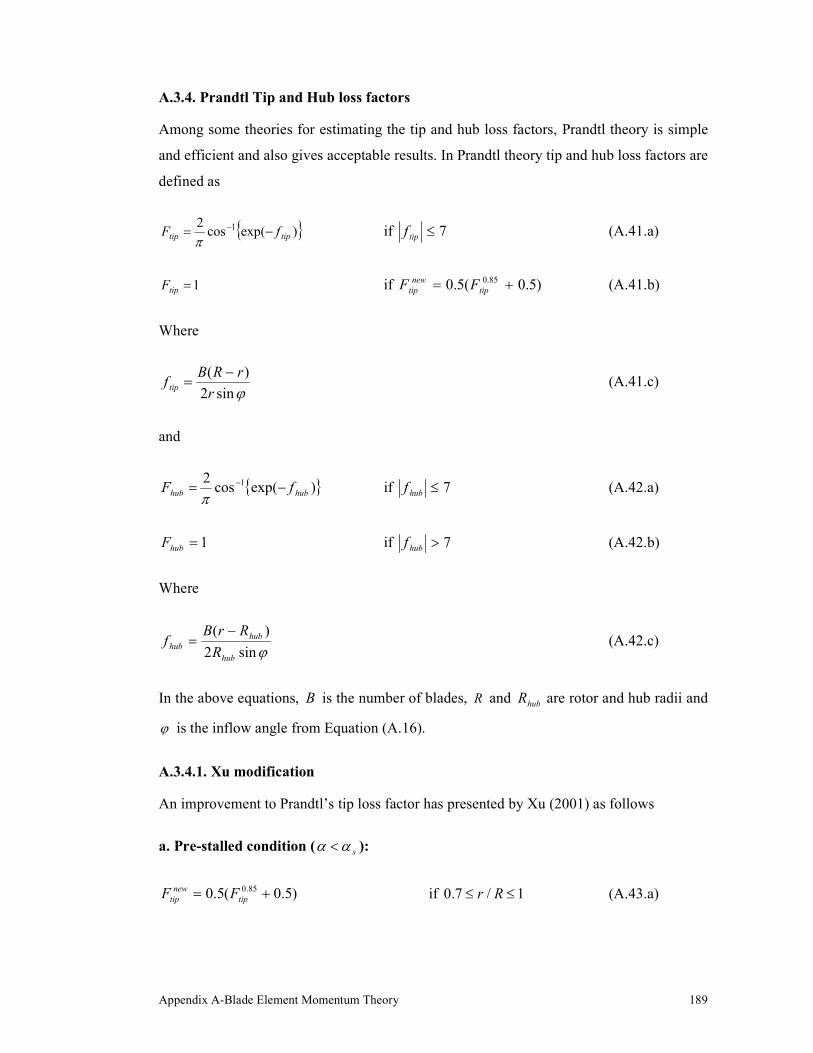
A.3.4. Prandtl Tip and Hub loss factors
Among some theories for estimating the tip and hub loss factors, Prandtl theory is simple
and efficient and also gives acceptable results. In Prandtl theory tip and hub loss factors are
defined as
)exp(cos2 1
tiptip fF −= −
π if 7≤tipf (A.41.a)
1=tipF if )5.0(5.0 85.0 += tip
new
tip FF (A.41.b)
Where
ϕsin2
)(
r
rRBf tip
−= (A.41.c)
and
)exp(cos2 1
hubhub fF −= −
π if 7≤hubf (A.42.a)
1=hubF if 7>hubf (A.42.b)
Where
ϕsin2
)(
hub
hub
hubR
RrBf
−= (A.42.c)
In the above equations, B is the number of blades, R and hubR are rotor and hub radii and
ϕ is the inflow angle from Equation (A.16).
A.3.4.1. Xu modification
An improvement to Prandtl’s tip loss factor has presented by Xu (2001) as follows
a. Pre-stalled condition ( sαα < ):
)5.0(5.0 85.0 += tip
new
tip FF if 1/7.0 ≤≤ Rr (A.43.a)

Appendix A-Blade Element Momentum Theory 190
R
FrF
Rrtipnew
tip7.0
)|1(1
7.0/ =−−= if 7.0/ <Rr (A.43.b)
b. Post-stalled condition ( sαα ≥ ):
8.0=new
tipF if 1/8.0 ≤≤ Rr (A.43.c)
1=new
tipF if 8.0/ <Rr (A.43.d)
A.3.5. Heavy loading (High axial induction factor)
Momentum theory predicts a parabolic variation for thrust coefficient with a maximum
value of 1 at 5.0=a , while the experimental data show that TC keeps increasing for
5.0>a . For small axial induction factors, 4.00 ≅<< caa , known as light loading state,
predicted thrust coefficient by the momentum theory is in a good agreement with the
experimental data. In the case of heavy loading state, where caa > , predicted TC departs
dramatically from its actual value. In the extreme loading situation, 1=a , wind turbine acts
as a drag driven device with a thrust coefficient of 2)( max, == DragTT CC rather than
0=TC as predicted by Equation (A.25). Extrapolating Equation (A.25), with a maximum
value of 2=TC at 1=a , predicts reasonable values for TC . Separating light and heavy
loading state, Equations (A.35) and (A.38) can be re-written as follows
a. Classical model
)1(4 aFFaCT −= if caa ≤ (A.44.a)
21
2
0 AaAaACT ++= if caa > (A.44.b)
where
2
2
0)1(
)2(442
c
cc
a
aaFFA
−
−+−= (A.44.c)
2
22
1)1(
8)1(44
c
ccc
a
aFaFaA
−
−++−= (A.44.d)

Appendix A-Blade Element Momentum Theory 191
2
2222
2)1(
442
c
ccc
a
aFFaaA
−
+−= (A.44.e)
b. Wilson-Walker model
)1(4 aFaCT −= if caa ≤ (A.45.a)
21
2
0 BaBaBCT ++= if caa > (A.45.b)
where
Fa
Bc
4)1(
220 −
−= (A.45.c)
Fa
aB
c
c 4)1(
421 +
−
−= (A.45.d)
22)1(
242
c
c
a
aB
−
−+= (A.45.e)
A.4. Blade Element Force Analysis
Figure (A.10) shows a blade segment (element) subjected to the aerodynamic forces in the
same system of coordinates as introduced in Figure (A.1). Assuming 2-dimentional flow
on the aerofoil and neglecting radial forces on the blade ( 0=sdF ), thrust force on the
element can be obtained as δcosndFdT = or
( ) δϕϕ cossincos dDdLdT += (A.46)
Lift and drag coefficients are defined as
( ) etn
rel
L
dAV
dLC
−
=2
21 ρ
(A.47)
( ) etn
rel
D
dAV
dDC
−
=2
21 ρ
(A.48)

Appendix A-Blade Element Momentum Theory 192
Figure A.10- Blade element force analysis
where ( )tnrelV − is the relative velocity in the tn − plane (see Figures (A.2) and (A.3)) and
δcoscdrcdsdAe == is the element area. Combining Equations (A.46), (A.47) and (A.48)
gives thrust force on a blade element as
( ) ( )drCCVcdT DLtnrel ϕϕρ sincos2
1 2 += − (A.49)
and for a turbine with B blades it becomes
( ) ( )drCCVBcdT DLtnrel ϕϕρ sincos2
1 2 += − (A.50.a)
or in terms of span coordinate
( ) ( ) δϕϕρ cossincos2
1 2dsCCVBcdT DLtnrel += − (A.50.b)
Using Equations (A.24) and (A.17), thrust coefficient can be written as
( )ϕ
ϕϕδσ2
22
sin
sincos)1(cos DLrT
CCaC
+−= (A.51)
where rσ , local solidity ratio, is defined as
δππσ
cos22 s
Bc
r
Bcr == (A.52)
Rotor Plane
Element
Blade Span
ϕ dD
tdF dL
ndF n
sdF
δ
dT
s
t
ndF δ
x
r

Appendix A-Blade Element Momentum Theory 193
Aerodynamic forces on the blade element also produce a torque about the rotor axis equal
to tx rdFdM = (Figure (A.10)). Recalling Equations (A.47) and (A.48), for a turbine
with B blades the generated torque about the rotor axis can be expressed as
( ) ( ) δϕϕρ coscossin2
1 2rdrCCVBcdM DLtnrelx −= − (A.53.a)
or in terms of span coordinate
( ) ( ) δϕϕρ coscossin2
1 2sdsCCVBcdM DLtnrelx −= − (A.53.b)
Inserting the above result into the definition of the torque coefficient MC , Equation (A.29),
yields to
( )ϕ
ϕϕδσ2
23
sin
cossin)1(cos DLrM
CCaC
−−= (A.54)
A.4.1. Blade Aerodynamic Characteristics
Lift and drag coefficients are functions of the angle of attack and Reynolds number. Angle
of attack is in turn a function of the velocity field and the blade geometry and can be
expressed as
αββϕα ∆+−−+= pitche 0 (A.55)
In the above equationϕ is the inflow angle, (Equation (A.16)), eβ and 0β stand for the
blade elastic twist and pre-twist, pitch is the blade pitch angle and α∆ accounts for the
angle of attack corrections as given by the following equation.
mc ααα ∆+∆=∆ (A.56)
In Equation (A.56) cα∆ refers to cascade correction and mα∆ refers to the other corrections.
A.4.1.1. Cascade Correction, cα∆
Cascade correction to the angle of attack has two components
21 ααα ∆+∆=∆ c (A.57)

Appendix A-Blade Element Momentum Theory 194
where 1α∆ accounts for the effect of finite aerofoil thickness and 2α∆ accounts for the
effect of finite aerofoil width
rc
AB a
πϕ
α2
cos 0
1 =∆ (A.58)
−
−′+
−=∆ −−
R
ra
Ra
ra )1(tan
)21(
)1(tan
4
1 11
2α (A.59)
0ϕ is the inflow angle prior to rotational induction, ( 0=′a in Figure (A.3)) and aA is the
aerofoil cross section area, normally taken as max68.0 ctAa ≈ , where maxt is the maximum
thickness of the aerofoil.
A.4.1.2. Effect of Finite Aspect Ratio, Pre-Stall Condition
The effect of finite aspect ratio at small angle of attacks can be considered as either
Estimating the finite aerofoil data by applying Lanchester-Pradtl theory to 2-D data
LL CC ′= (A.60)
AR
CCC L
DD π
2
+′= (A.61)
AR
CL
παα +′= (A.62)
where LC ′ , DC ′ and α ′ are infinite aerofoil data and AR stands for the aspect ratio, or using
2-D data and applying a tip loss factor to the HAWT aerodynamic model.
A.4.1.3. Effect of Finite Aspect Ratio, Post-Stall Condition
For larger angle of attacks, two models can be used to estimate lift and drag coefficients of
an aerofoil.
a. Viterna-Corrigan model
Viterna-Corrigan model (Viterna and Corrigan, 1981) uses only three values from the 2-
Dim data to estimate lift and drag coefficients in post-stall condition, 90<<αα s .

Appendix A-Blade Element Momentum Theory 195
αα
ααsin
coscossin
2
max, LDL KCC += (A.63)
αα cossin 2
max, DDD KCC += (A.64)
where
( )s
s
ssDstallLL CCKαα
αα2max,,
cos
sincossin−= (A.65)
s
sDstallD
D
CCK
α
α
cos
sin 2
max,, −= (A.66)
ARCD 018.11.1max, += if 50≤AR (A.67.a)
01.2max, =DC if 50>AR (A.67.b)
For other angle of attacks in the range of [-180, 180] reflected values for DC and reflected-
reduced values for LC can be used, (see Figure (A.11)).
b. Flat-Plate Theory
Flat-plate theory estimates post-stall aerodynamic characteristics of an aerofoil as
αcosNL CC = (A.68)
αsinND CC = (A.69)
where
+= 98.1,
sin
238.0222.0
1min
α
NC if 1≥F (A.70.a)
−−=
F
FCN
2
)1(22.12tanh81.098.1 if 15.0 << F (A.70.b)

Appendix A-Blade Element Momentum Theory 196
17.1=NC if 5.0≤F (A.70.c)
-1
-0.5
0
0.5
1
1.5
-180 -150 -120 -90 -60 -30 0 30 60 90 120 150 180
Angle of attack
AD C B C D
Drag
Lift
A: Available data
B: Viterna model
C: Viterna model with reflection and reduction
D: Interpolation between limits
Figure A.11- Viterna post-stall model
A.5. Blade Element Momentum Theory, BEMT
Equating thrust and torque coefficients obtained from the blade element force analysis
(with the assumption of zero drag force) and those obtained from momentum theory is the
base of the BEMT. Neglecting drag force in Equations (A.51) and (A.54), thrust and torque
coefficients will become
ϕϕδσ
2
22
sin
cos)1(cos0
LrT
CaC
−= (A.71)
ϕϕδσ
2
22
sin
sin)1(cos0
LrM
CaC
−= (A.72)
Depending on which brake state model in the momentum theory is used, formulation for
BEMT will be different.
a. Classical Model
Combining Equations (A.71) and (A.72) with equations (A.44) and (A.36) gives

Appendix A-Blade Element Momentum Theory 197
2
110T
Ca
−−= if 96.04.0
0≤≡≤ TCa (A.73.a)
0
20
2
11
2
)(40
A
CAAAAa
T−−+−= if 96.04.0
0>≡> TCa (A.73.b)
δλϕ
cos
tan
r
aFa =′ (A.74)
b. Wilson-Walker Model
Combining Equations (A.71) and (A.72) with Equations (A.45) and (A.39) gives:
2
11 0
F
C
a
T−−= if FCa T 96.04.0
0≤≡≤ (A.75.a)
0
20
2
11
2
)(40
B
CBBBBa
T−−+−= if FCa T 96.04.0
0>≡> (A.75.b)
δλϕ
cos
tan
r
aa =′ (A.76)
6 Equations (A.16), (A.31), (A.55), (A.71), (A.73)/(A.75), (A.74)/(A.76) and two set of
tabulated data for LC and DC can be solved to find a , a ′ , F ,ϕ ,α , LC , DC and 0T
C .
Knowing a ,ϕ , LC and DC one can use Equations (A.50) and (A.51) to calculate T and
TC and Equations (A.53) and (A.54) to find M and MC . Having rotor torqueM , turbine
mechanical power, P can be easily calculated by
MdMP Ω=Ω= ∫ (A.77)
and the power coefficient PC can be determined from the following equation.
233
21
21 RV
P
AV
PC
wrotorw
P
πρρ== (A.78)

Appendix A-Blade Element Momentum Theory 198
A.6. Flap bending
Referring to Figure (A.12), tangential and normal force increments on the blade element at
locationη , tdF and ndF , are given by Equation (A.79).
( )ηηη
ϕϕϕϕ
ηρϕϕϕϕ
.
2
..sincos
cossin
21
sincos
cossin
atD
L
tnrel
atatn
t
C
CdVc
dD
dL
dF
dF
−=
−=
−
(A.79)
Figure A.12- Blade element force analysis for flap bending calculation
Flap-bending moment produced by these forces at location s can be calculated as:
( ) ( ) ( )( )∫−=
=
−−+=s
R
ntsatFB sR
dFdFM δη
η ηη ηδ
ξξcos
0.cos
sincos (A.80)
In the above equation,
−− sR
ηδcos
is the moment arm and ξ is the angle between the
normal axis and the chord line at s - location which can be expresses in terms of the inflow
and attack angles as:
sat.)( αϕξ −= (A.81)
r
Blade
element
δ
s
η
x
R
ϕ
dD
dL
n
t
Chord line at
s -location
ξ
ndF
tdF
Appendix A-Blade Element Momentum Theory 199
A.7. References
Tulapurkara, E.G., 1996. Turbulence Models for the Computation of Flow past Airplanes.
Progress in Aerospace Sciences, 33, pp 71-165.
Viterna, L.A., Corrigan, R.D., 1981. Fixed Pitch Rotor Performance of Large Horizontal
Axis Wind Turbines. In: DOE/NASA workshop on Large HAWT's, Cleveland, Ohio, 1981.
Xu, G., 2001. Computational Studies of Horizontal Axis Wind Turbines. Doctoral Thesis,
Georgia Institute of Technology.