appendix b5 supplemental streamflow...

Appendix B5 Supplemental Streamflow Analysis

Appendix B5 — Supplemental Streamflow Analysis

The streamflow analyses presented in this appendix provide additional supporting information consistent with that provided in the Technical Report. The streamflow analysis, as described here, was based on reconstructed natural flows in the Colorado River Basin (Basin). The data consist of two historical datasets. The first dataset (referred to as the observed record) consists of monthly observed natural flows for the period October 1905 to September 2007. The second dataset (referred as the paleo record) consists of monthly flows reconstructed from tree ring analysis for the period October 761 to September 2005.

The observed record was provided in the total flows format (flows accumulating from upstream to downstream locations) and intervening format (single watershed flows). The paleo record was provided in an intervening format and had to be accumulated from upstream to downstream basins to obtain a total flows format.

1.0 Streamflow Data Summary Streamflow was analyzed for the 29 natural flow stations that serve as the primary inflow locations for the Colorado River Simulation System model. A spreadsheet tool was constructed to provide an interactive environment to explore the temporal and spatial characteristics of streamflow in the Basin, as shown in figure B5-1. The features of this visual summary are described as follows:

A. Table of Statistics: The table includes statistics (Stat1 and Stat2) for two periods in columns that represent the absolute and percentage difference between the two time periods. The Stat1 and Stat2 columns present the long-term water year streamflow average for the two periods. The “Annual” statistic block shows the minimum and the maximum observed for the 1-year totals and 3-, 5-, 10-, 20-, and 30-year moving averages, followed by the year that the value was observed (e.g., the line “3yr Min (WYear) 7370 (1847)” represents a minimum value of 7,370 thousand acre-feet (kaf) per year for a 3-year moving average time series ending in the year of 1847). The “Monthly statistics” section shows the monthly streamflow averages for each month, followed by the seasonal statistics (average, standard deviation, and amplitude [maximum-minimum]). The amplitude accounts for all seasons; for example, for amplitude October, November, and December (OND), the value on the table is computed as the maximum flow observed in an OND season minus the minimum flow observed in an OND season. The minimum and the maximum do not necessarily occur in the same water year.

B. Average Monthly Streamflow Graphic: Average monthly streamflow (kaf) is shown for the water year over the time periods. The data used for this plot are also presented in the Table of Statistics as Stat1 (solid line) and Stat2 (dashed line). This graphic can be used to assess monthly and seasonal shifts in streamflow from the comparison periods.

December 2012 B5-1

Colorado River Basin Water Supply and Demand Study

FIGURE B5-1 Summary Graphic for Colorado River at Lees Ferry, Arizona Displaying Streamflow, Annual Exceedance Probabilities, Streamflow Deficits and Surpluses, and Drought Duration, Magnitude and Intensity

B

A C

E F

H

G

D

B5-2 December 2012


December 2012 B5-3

C. Annual Streamflow Box and Whiskers Graphic: This plot illustrates annual streamflow variability for the two time periods. The box represents the range of half of annual observed flows (inter-quartile range between 25th and 75th percentile). The triangle represents the median, and the horizontal lines at the top of the vertical line represent the period of record maximum and minimum annual values. This graphic can be used to assess trends in period streamflow variability and volumes.

D. Table of Statistics: The table includes statistics (Stat1 and Stat2) for two periods in columns that represent the absolute and percentage difference between the two time periods. The Stat1 and Stat2 columns present the long-term water year streamflow average for the two periods. The “Annual” statistic block shows the minimum and the maximum observed for the 1-year totals and 3-, 5-, 10-, 20-, and 30-year moving averages, followed by the year that the value was observed (e.g., the line “3yr Min (WYear) 7370 (1847)” represents a minimum value of 7,370 kaf per year for a 3-year moving average time series ending in the year of 1847). The “Monthly statistics” section shows the monthly streamflow averages for each month, followed by the seasonal statistics (average, standard deviation, and amplitude [maximum-minimum]). The amplitude accounts for all seasons; for example, for amplitude October, November, and December (OND), the value on the table is computed as the maximum flow observed in an OND season minus the minimum flow observed in an OND season. The minimum and the maximum do not necessarily occur in the same water year.

E. Average Monthly Streamflow Graphic: Average monthly streamflow (kaf) is shown for the water year over the time periods. The data used for this plot are also presented in the Table of Statistics as Stat1 (solid line) and Stat2 (dashed line). This graphic can be used to assess monthly and seasonal shifts in streamflow from the comparison periods.

F. Annual Streamflow Box and Whiskers Graphic: This plot illustrates annual streamflow variability for the two time periods. The box represents the range of half of annual observed flows (inter-quartile range between 25th and 75th percentile). The triangle represents the median, and the horizontal lines at the top of the vertical line represent the period of record maximum and minimum annual values. This graphic can be used to assess trends in period streamflow variability and volumes.

G. Annual Streamflow Exceedance Graphic: This plot presents the full range of probabilities of exceeding a given streamflow for two selected periods. The plot is equivalent to the box and whiskers plot but provides probabilities ranging from zero to 100 percent. This graphic can be used to assess trends in period streamflow variability and volumes. For example, at the Lees Ferry, Arizona, location, 90 percent of the years had streamflows exceeding 10,000 kaf for both periods.

H. Deficit Related Statistics – Exceedance Plots: The deficit statistics are illustrated in three charts: duration, magnitude, and intensity. The statistics presented in these charts refer only to deficit periods defined as only the years when streamflows were below the specified threshold. The “percentage of all years in a deficit” takes into account all years in the time period and determines how many were within a “deficit.” Below is a more detailed description of the deficit related statistics.

The average streamflow for each time period is the default threshold to define deficit or surplus periods (e.g., a sequence of years with streamflows below the average is considered a deficit period).

Duration: The duration chart presents the exceedance probability of deficit duration in years. For example, the chart illustrates that at Lees Ferry, 30 percent of the years defined as deficit years (only deficit years) had a deficit that lasted or exceeded 3 years in duration.

Magnitude: The magnitude of a deficit (kaf) corresponds to the cumulative difference between observed streamflows and long-term average streamflows for an uninterrupted drought period. The exceedance plot shows the probability of a deficit to exceed a certain magnitude based on observed flows.

Intensity: Deficit intensity is presented as magnitude divided by duration. The chart presents the exceedance probabilities for two selected periods.

2.0 Streamflow Data Summaries Sample streamflow data summaries are provided in the following pages for the following natural flow stations:

Figure B5-2: Colorado River at Lees Ferry, Arizona (Station 20) Figure B5-3: Green River at Green River, Utah (Station 16) Figure B5-4: Colorado River near Cisco, Utah (Station 8) Figure B5-5: San Juan River near Bluff, Utah (Station 19) Figure B5-6: Colorado River above Imperial Dam, Arizona (Station 29)


B5-4 December 2012


FIGURE B5-2 Streamflow Data Summary for Colorado River at Lees Ferry, Arizona, Natural Flows Based on historical 1906–2007 data.

December 2012 B5-5


FIGURE B5-3 Streamflow Data Summary for Green River at Gre en River, Utah, Natural Flows Based on historical 1906–2007 data.

B5-6 December 2012


FIGURE B5-4 Streamflow Data Summary for Colorado River near Cisco, Utah, Natural Flows Based on historical 1906–2007 data.

December 2012 B5-7


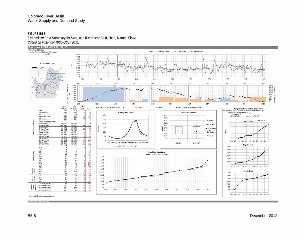
FIGURE B5-5 Streamflow Data Summary for San Juan River near Bluff, Utah, Natural Flows Based on historical 1906–2007 data.

B5-8 December 2012


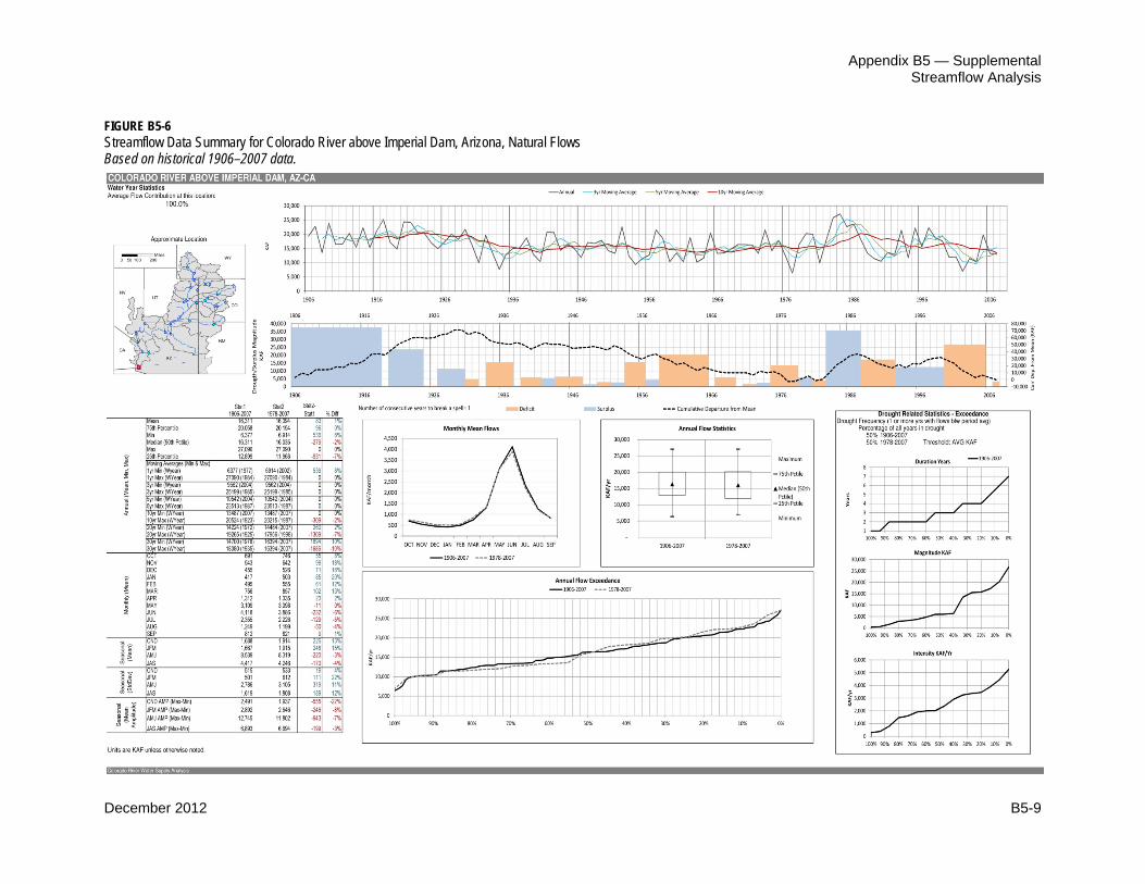
FIGURE B5-6 Streamflow Data Summary for Colorado River above Imperial Dam, Arizona, Natural Flows Based on historical 1906–2007 data.

December 2012 B5-9

appendix b5 supplemental streamflow...

Documents