appendix b step-by-step applications of the...

98

APPENDIX B

STEP-BY-STEP APPLICATIONS OF THE FEMWATER-LHS

Steady Two-Dimensional Drainage Problem

1. Double-click on the Argus ONE icon to open Argus ONE.

2. From the PIEs menu found along the top of the window, select, New FEMWATERProject.... This brings up the FEMWATER-LHS Type of Simulation Problem window.

3. Here, the type of problem to be simulated is chosen. To select the type of CROSS-SECTIONAL click on check box and then click Continue. The FEMWATER-LHS Modeldialog appears.

4. This window allows the user to specify values for the FEMWATER simulation that are

not spatially variable. This dialog can be get again at any time by selecting PIEs|EditProject Info. Rather than making changes here now, accept the default values by clicking

OK. This brings up a new Argus ONE window, called “untitled1”.

5. This is the window in which the model will be designed, run, and evaluated. It contains

many layers in a stack; each layer will hold either model or mesh information.

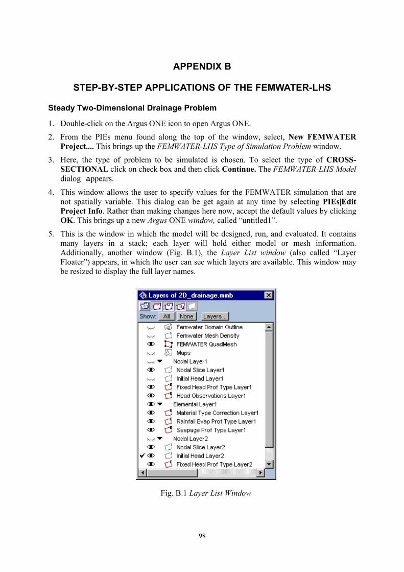
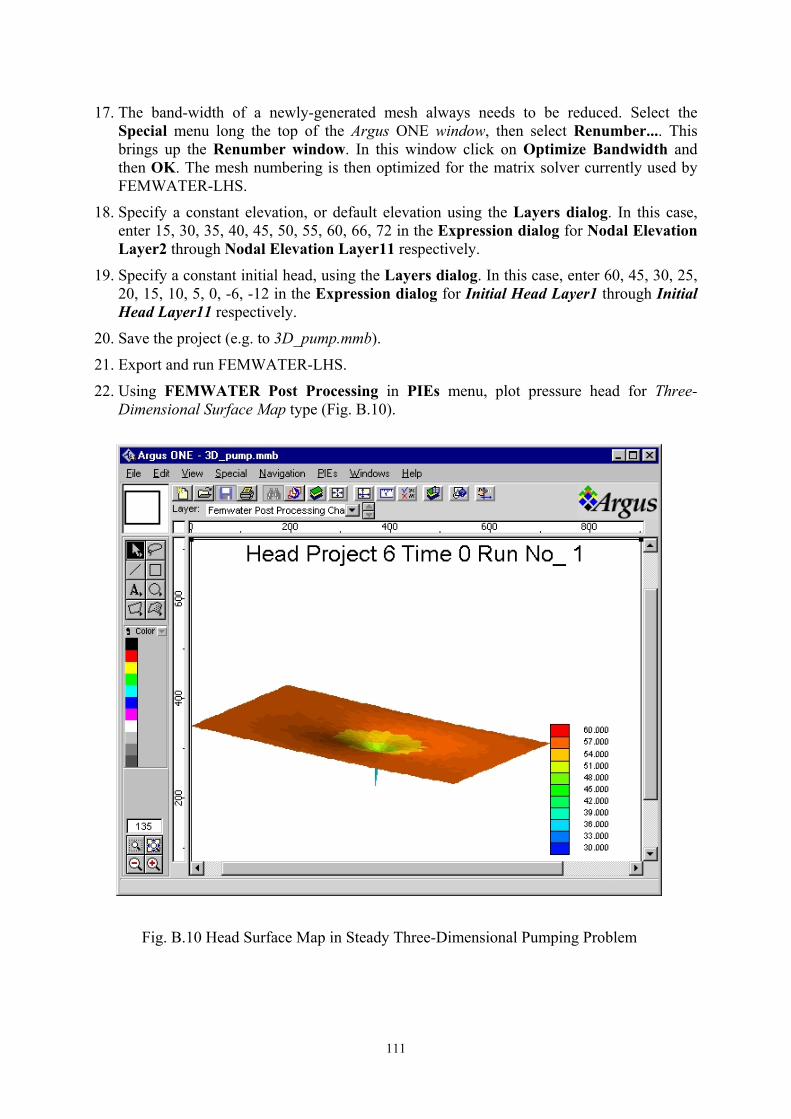
Additionally, another window (Fig. B.1), the Layer List window (also called “Layer

Floater”) appears, in which the user can see which layers are available. This window may

be resized to display the full layer names.

Fig. B.1 Layer List Window

99

The Layer List window shows which information layers are available for the particularproblemtype, i.e. Nodal Elevation Layer[i] or Nodal Slice Layer[i], Initial HeadLayer[i], Material Type Correction Layer[i], etc. The window allows the user to controlwhich of the layers will be visible (those with the open eye) and which layer is on top ofthe stack and thus available for input from the screen. Clicking on an ‘eye’ toggles thelayer visibility, and clicking to the left of an ‘eye’ makes the layer ‘active’ (i.e. brings thelayer to the top of the stack) and puts a ‘check mark’ next to the active layer.

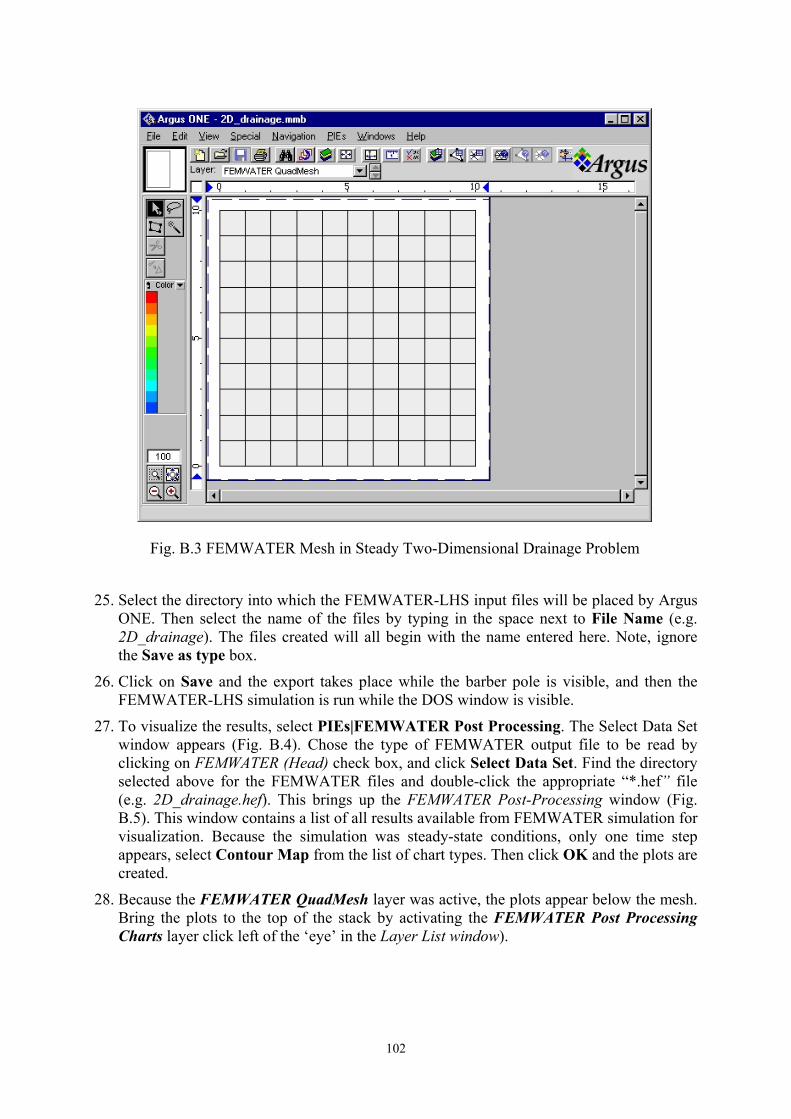
6. To create a rectangular uniform elements. It is possible to read a Grid (rectangularuniform elements) into FEMWATER Quadmesh directly. However, mesh BandWidthcan be minimized once the mesh is imported. A text file (e.g. 2D_drainage_mesh.exp)containing 100 elements and 121 nodes was used to represent the flow region. Activatethe FEMWATER Quadmesh by clicking to the left of its ‘eye’ in the Layer List window.Import 2D_drainage_mesh.exp into the project by selecting File|Import FEMWATERQuadMesh...|Text File. In CD-ROM, the 2D_drainage_mesh.exp file is located in adirectory with the pathname examples\application_1\app1_import_files\.

7. To specify a constant slice position, or default slice position for the nodal of layer, theLayers dialog must be used. Moving the cursor to the Layers... button in the floatinglayers window and clicking, opens the Layers dialog. The list at the top of the dialog is thelist of layers. Highlighting the layer under consideration, in this case Nodal Slice Layer2,in that list by clicking it with the cursor shows the parameters associated with thatinformation layer in the table at the bottom of the dialog box. Moving the cursor to theValue column and clicking fx the expression box to appear. Just type 10 in the expressionbox and clicking OK exits the expression dialog.

8. To modify the non-spatial data (i.e. boundary conditions profile types and materialcorrection types) in this project. Select PIEs|Edit Project Info, the FEMWATER-LHSModel dialog will appear.

9. Click on Material and Soil Properties tab to activate material correction by clickingMaterial type correction check box and set the following parameters:

On Correction Cond/Perm tab, set

N xx yy Zz xy xz yz1 0.06 0.0 0.06 0.0 0.0 0.0

On Correction Soil Prop tab, set

N Res MC Sat MC P Head VG Alpha VG Beta1 0.034 0.046 0.0 1.6 1.37

10. Click on the Boundary Conditions|Dirichlet tab to activate fixed head profile type byclicking Fixed Head check box. Enter the values of the profile. Specify 2 m for the headin unlimited time, enter the same values of Head 1 and Head 2 with 2, Time 1 with 0 andTime 2 with the 1.0e38.

11. Click on the Boundary Conditions|Variable Composite tab to activate rain fall and see-page profile type by clicking Rainfall/Evap-Seepage check box. Enter the values of thefirst profile. Specify 0.006 m/day for the rain fall in unlimited time, enter the same valuesof Rf/Evap 1 and Rf/Evap 2 with 0.006, Time 1 with 0 and Time 2 with the 1.0e38. Addthe number of profiles by clicking on the Add Rows button. Enter the values of thesecond profile. There are the same values of Rf/Evap 1 and Rf/Evap 2 with 0.0 in

100

unlimited time (Time 1 with 0 and Time 2 with the 1.0e38). Thus, there are two types(number 1 and number 2) rain fall and see-page boundary conditions. Finally clicking OKto finish the changes.

12. To enter the Dirichlet boundary conditions into the model, activate the Fixed Head ProfType Layer1, by clicking on its ‘eye’ in the Layer List window.

13. Draw a line by first activating the contour-drawing tool. To do this, click on the smallquadrilateral just below the arrow along the left side of the Argus ONE window and selectthe Open Contour Tool from the pop-up menu. It is the middle item. Now draw a verticalline through the nodes in bottom left of the model and assign it a Fixed Head Prof Typeto 1.

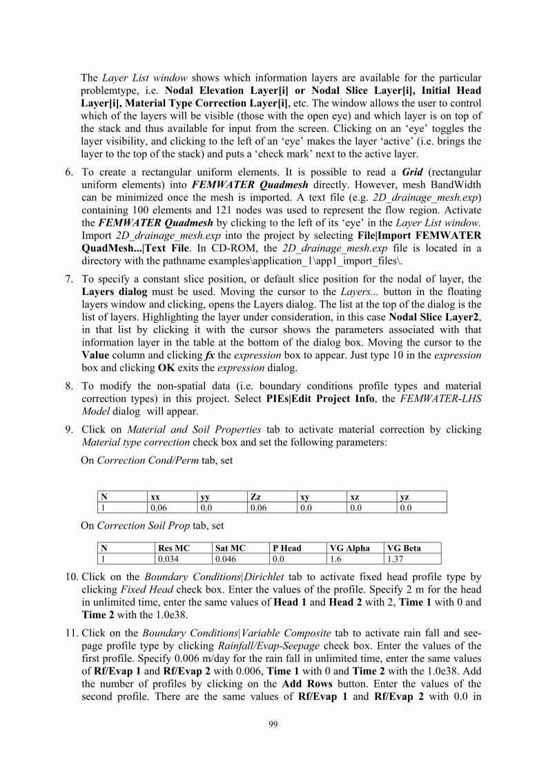
14. To set the precise node positions using EditContours. Select File|Import FemwaterDomain Outline|Edit Contours. Then select the Fixed Head Prof Type Layer1 from thelist of layers. The objects on the Fixed Head Prof Type Layer1 will be imported into theEditContours PIE. Click on any node there to select it and edit it's position (Fig. B.2).

15. Copy this contour by pressing Ctrl+C or select Edit|Copy.

16. Activate the Fixed Head Prof Type Layer2, by clicking on its ‘eye’ in the Layer Listwindow. Select Edit|Paste to create this contour. Paste in the copied object by pressingCtrl+V (or select Edit|Paste).

17. To enter the Rainfall/Evaporation boundary conditions into the model, activate theRainfall Evap Prof Type Layer1, by clicking on its ‘eye’ in the Layer List window.

Fig. B.2 EditContours dialog

101

18. Click on the small quadrilateral just below the arrow along the left side of the Argus ONEwindow and select the Open Contour Tool from the pop-up menu. It is the middle item.Draw a horizontal line through the top row elements and set:

Rainfall Evap Prof Type = 1Ponding Depth = 0Min Pressure Head = -9000

and click OK.

19. To enter the Seepage boundary conditions into the model, activate the Seepage Prof TypeLayer1, by clicking on its ‘eye’ in the Layer List window.

20. Draw a vertical line through the 8 elements on the left edge of the model and set:

Seepage Prof Type = 2Ponding Depth = 0Min Pressure Head = -9000

and click OK.

21. To enter the material correction type into the model, activate the Material TypeCorrection Layer1, by clicking on its ‘eye’ in the Layer List window.

22. Click on the small quadrilateral just below the arrow along the left side of the Argus ONEwindow and select the Close Contour Tool from the pop-up menu. It is the first item.Draw a polygon through the 3 rows of element on the top of the model and assign it aMaterial Type to 1.

23. Save the project so far by clicking File, and then Save As.... Select the desired directoryand type in the desired name (e.g. 2D_drainage) and then click on Save. A project filecalled 2D_drainage.mmb is created in the directory you chose, and the window namebecomes the same, as shown in Fig. B.3.

24. The model information entered now needs to be exported from Argus ONE creating inputfiles that FEMWATER-LHS requires, and the simulation can then be run. (Note that theFEMWATER QuadMesh layer must be active in order to export.) In the PIEs menu,select Run FEMWATER. The Run FEMWATER dialog box appears.

The full paths to the executables should be displayed in edit-boxes on the FEMWATERPath the Run FEMWATER dialog box. If the executable for the chosen model is not atthe location specified in the edit-box, the background of the edit-box and the status barwill change to red and a warning message will be displayed in the status bar to indicatethat the path is incorrect. Normally, the user should correct the path before attempting tocreate the input files. Although it is possible to export the input files using an incorrectpath. Argus ONE will not be able to start the model if the path is incorrect. Type thecorrect path or click on the Browse button to set the correct path. When a model is saved,the paths for all of the models will be saved in a file named Femwater_lewaste_lhs.ini inthe directory containing the FEMWATER PIE. Femwater_lewaste_lhs.ini will be readwhenever a new FEMWATER project is created or an old one is read so that the modelpaths do not need to be reset frequently. In this windows also allows the user to chooseonly creation of FEMWATER-LHS input files, or both creation of files and running ofFEMWATER-LHS (which is already selected). Click OK to proceed. An Enter export filename window appears.

102

25. Select the directory into which the FEMWATER-LHS input files will be placed by Argus

ONE. Then select the name of the files by typing in the space next to File Name (e.g.

2D_drainage). The files created will all begin with the name entered here. Note, ignore

the Save as type box.

26. Click on Save and the export takes place while the barber pole is visible, and then the

FEMWATER-LHS simulation is run while the DOS window is visible.

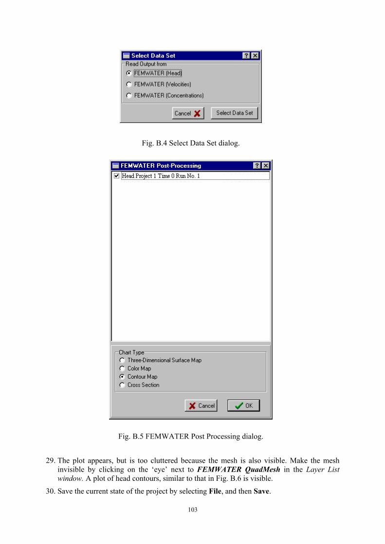
27. To visualize the results, select PIEs|FEMWATER Post Processing. The Select Data Set

window appears (Fig. B.4). Chose the type of FEMWATER output file to be read by

clicking on FEMWATER (Head) check box, and click Select Data Set. Find the directory

selected above for the FEMWATER files and double-click the appropriate “*.hef” file

(e.g. 2D_drainage.hef). This brings up the FEMWATER Post-Processing window (Fig.

B.5). This window contains a list of all results available from FEMWATER simulation for

visualization. Because the simulation was steady-state conditions, only one time step

appears, select Contour Map from the list of chart types. Then click OK and the plots are

created.

28. Because the FEMWATER QuadMesh layer was active, the plots appear below the mesh.

Bring the plots to the top of the stack by activating the FEMWATER Post ProcessingCharts layer click left of the ‘eye’ in the Layer List window).

Fig. B.3 FEMWATER Mesh in Steady Two-Dimensional Drainage Problem

103

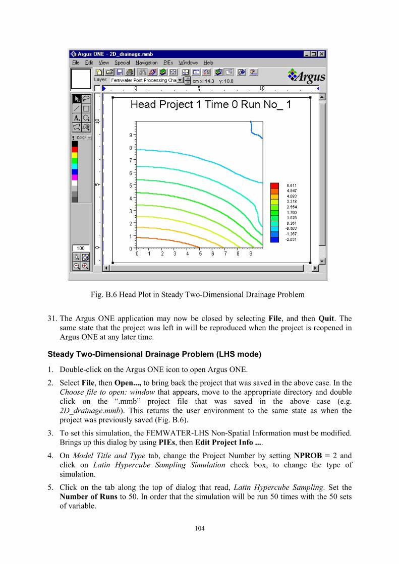
29. The plot appears, but is too cluttered because the mesh is also visible. Make the meshinvisible by clicking on the ‘eye’ next to FEMWATER QuadMesh in the Layer Listwindow. A plot of head contours, similar to that in Fig. B.6 is visible.

30. Save the current state of the project by selecting File, and then Save.

Fig. B.4 Select Data Set dialog.

Fig. B.5 FEMWATER Post Processing dialog.

104

31. The Argus ONE application may now be closed by selecting File, and then Quit. Thesame state that the project was left in will be reproduced when the project is reopened inArgus ONE at any later time.

Steady Two-Dimensional Drainage Problem (LHS mode)


2. Select File, then Open..., to bring back the project that was saved in the above case. In theChoose file to open: window that appears, move to the appropriate directory and doubleclick on the “.mmb” project file that was saved in the above case (e.g.2D_drainage.mmb). This returns the user environment to the same state as when theproject was previously saved (Fig. B.6).

3. To set this simulation, the FEMWATER-LHS Non-Spatial Information must be modified.Brings up this dialog by using PIEs, then Edit Project Info ....

4. On Model Title and Type tab, change the Project Number by setting NPROB = 2 andclick on Latin Hypercube Sampling Simulation check box, to change the type ofsimulation.

5. Click on the tab along the top of dialog that read, Latin Hypercube Sampling. Set theNumber of Runs to 50. In order that the simulation will be run 50 times with the 50 setsof variable.

Fig. B.6 Head Plot in Steady Two-Dimensional Drainage Problem

105

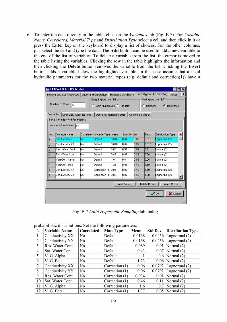
6. To enter the data directly in the table, click on the Variables tab (Fig. B.7). For VariableName, Correlated, Material Type and Distribution Type select a cell and then click in it orpress the Enter key on the keyboard to display a list of choices. For the other columns,just select the cell and type the data. The Add button can be used to add a new variable tothe end of the list of variables. To delete a variable from the list, the cursor is moved tothe table listing the variables. Clicking the row in the table highlights the information andthen clicking the Delete button removes the variable from the list. Clicking the Insertbutton adds a variable below the highlighted variable. In this case assume that all soilhydraulic parameters for the two material types (e.g. default and correction(1)) have a

probabilistic distributions. Set the following parameters:N Variable Name Correlated Mat. Type Mean Std Dev Distribution Type1 Conductivity XX No Default 0.0168 0.0456 Lognormal (2)2 Conductivity YY No Default 0.0168 0.0456 Lognormal (2)3 Res. Water Cont. No Default 0.089 0.01 Normal (2)4 Sat. Water Cont. No Default 0.43 0.07 Normal (2)5 V. G. Alpha No Default 1 0.6 Normal (2)6 V. G. Beta No Default 1.23 0.06 Normal (2)7 Conductivity XX No Correction (1) 0.06 0.0792 Lognormal (2)8 Conductivity YY No Correction (1) 0.06 0.0792 Lognormal (2)9 Res. Water Cont. No Correction (1) 0.034 0.01 Normal (2)10 Sat. Water Cont. No Correction (1) 0.46 0.11 Normal (2)11 V. G. Alpha No Correction (1) 1.6 0.7 Normal (2)12 V. G. Beta No Correction (1) 1.37 0.05 Normal (2)

Fig. B.7 Latin Hypercube Sampling tab dialog

106

7. Click OK to exit the dialog. Save the project (e.g. to 2D_drainage_lhs.mmb).

8. To export and run, activate the FEMWATER QuadMesh layer again bringing the mesh tothe top of the stack. Select PIEs, and then Run FEMWATER.

9. Click OK in the Run FEMWATER window, and Select the directory into which theFEMWATER-LHS input files will be placed and select the name of the new files that willrun the LHS mode simulation (e.g. 2D_drainage_lhs). Note, ignore the Save as type box.Click on Save to export and run.

10. The results can be analyzed in statistically. However, the results can be visulaized. Fromthe PIEs menu select FEMWATER Post Processing. Click on FEMWATER (Head)

check box in the select data file dialog and click Select Data Set. Find the directoryselected above for the FEMWATER files and double-click the appropriate “*.hef” file(e.g. 2D_drainage_lhs.hef). The FEMWATER Post-Processing window will be appear.Select the data file and select Contour Map from the list of chart types. Then click OK

and the plots are created.

Transient Two-Dimensional Drainage Problem


2. Select File, then Open..., to bring back the project that was saved in the above case. In theChoose file to open: window that appears, move to the appropriate directory and doubleclick on the “.mmb” project file that was saved in the above case (e.g.2D_drainage.mmb). This returns the user environment to the same state as when theproject was previously saved.

3. In this case the region consist only one material type. There is no material correction exist.To modify this information, brings up the FEMWATER-LHS Non-Spatial Informationdialog by using PIEs, then Edit Project Info ....

4. On Model Title and Type tab, set NPROB = 3.

5. To change the type of solution, click on Run Control tab and click Transient StateSolution check box.

6. The transient simulation will be performed for 50 time steps. The initial time step size is0.25 day and each subsequent time step size is increased with a multiplier of 2.0 with themaximum time step size of less than or equal to 32 days. The pressure head tolerance fornonlinear iteration is 2 × 10-3 m. The relaxation factor for the nonlinear iteration is setequal to 0.5. To input this information, click on Time Control tab and set:

NTI = 50TMAX = 2000DELT = 0.25CHNG = 2.0DELMAX = 32

and click OK.

7. To delete or inactivate the material correction, click on Material and Soil Properties taband then clicking Material type correction check box.

8. In this simulation the initial conditions were used the steady state solution resulting fromzero flux on the top. However, this solution is already done that so it can be just importthose contours. Activate the Initial Head Layer1, by clicking on its ‘eye’ in the Layer List

107

window. Import 2D_drainage_init.exp into the project by selecting File|Import InitialHead Layer1|Text File, and then select 2D_drainage_init.exp.

9. Copy this contour by pressing Ctrl+C or select Edit|Copy.

10. Activate the Initial Head Layer2, by clicking on its ‘eye’ in the Layer List window. SelectEdit|Paste to create this contour. Paste in the copied object by pressing Ctrl+V (or selectEdit|Paste).

11. Save the project (e.g. to T_2D_drainage.mmb).

12. Export and run FEMWATER-LHS.

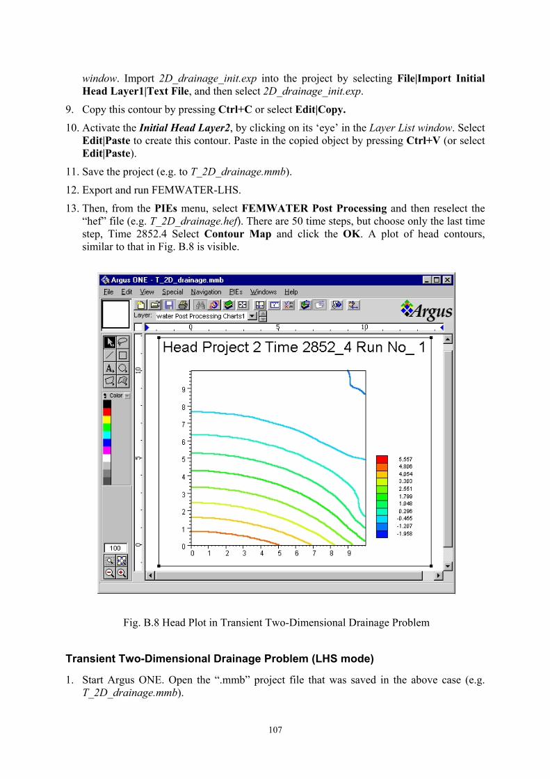
13. Then, from the PIEs menu, select FEMWATER Post Processing and then reselect the“hef” file (e.g. T_2D_drainage.hef). There are 50 time steps, but choose only the last timestep, Time 2852.4 Select Contour Map and click the OK. A plot of head contours,similar to that in Fig. B.8 is visible.

Transient Two-Dimensional Drainage Problem (LHS mode)

1. Start Argus ONE. Open the “.mmb” project file that was saved in the above case (e.g.T_2D_drainage.mmb).

Fig. B.8 Head Plot in Transient Two-Dimensional Drainage Problem

108

2. Select PIEs, then Edit Project Info ... to modify the the FEMWATER-LHS Non-SpatialInformation.

On Model Title and Type tab, set NPROB = 4 and click Latin Hypercube Sampling

Simulation check box

On Latin Hypercube Sampling tab, set the Number of Runs to 32

On Latin Hypercube Sampling|Variables tab, set the following parameters:

N Variable Name Correlated Mat. Type Mean Std Dev Distribution Type

1 Conductivity XX No Default 0.0168 0.0456 Lognormal (2)2 Conductivity YY No Default 0.0168 0.0456 Lognormal (2)3 Res. Water Cont. No Default 0.089 0.01 Normal (2)4 Sat. Water Cont. No Default 0.43 0.07 Normal (2)5 V. G. Alpha No Default 1 0.6 Normal (2)6 V. G. Beta No Default 1.23 0.06 Normal (2)

Then click OK.

3. Save the project (e.g. to T_2D_drainage_LHS.mmb).


5. Uncertainty and sensitivity analysis of the input and the output variables.

Steady Three-Dimensional Pumping Problem

1. Start Argus ONE. In the FEMWATER-LHS Type of Simulation Problem window, select aAreal orientation. Then click Continue.

2. In the FEMWATER-LHS dialog, a number of changes to the initial default values arerequired.

On Model Title and Type tab, set NPROB = 5

On Material and Soil Properties tab, click Material type correction check box and click

Add Rows button to add the number of correction material. Set the following parameters:

On Cond/Perm tab, set

xx yy zz xy xz yz0.3144 0.3144 0.3144 0.0 0.0 0.0

On Soil Prop tab, set

Res MC Sat MC P Head VG Alpha VG Beta0.1 0.39 0.0 5.8 1.48


N xx yy zz xy xz yz1 1.0608 1.0608 1.0608 0.0 0.0 0.02 7.128 7.128 7.128 0.0 0.0 0.0

109


N Res MC Sat MC P Head VG Alpha VG Beta1 0.065 0.41 0.0 7.5 1.892 0.045 0.43 0.0 14.5 2.68

On Layer and Calibration tab, click Add button 9 times to set the number of elemental

layers to 10 or the number of nodal layers to 11.

On the Boundary Conditions|Dirichlet tab, click Fixed Head check box and then click

Add Rows button to add the number of profile. Set the profiles as follows:

N Time 1 Head 1 Time 2 Head 21 0.0 60.0 1.0e38 60.02 0.0 30.0 1.0e38 30.0

3. In the Argus ONE window, select Special|Scale and Units... and set Uniform Scale: =50. That it reads “Every 1 cm on the screen represents 50 units in the real world in boththe x and y direction”.

4. Activate the Femwater Domain Outline layer and draw a model boundary with thecontour-drawing tool. Try to create a square outline with 1000 m wide and 400 m high.Then, double-click on the location desired for the last vertex. The Contour Informationdialog appears. Here the desired typical size of finite elements to be created by the meshgenerator is specified. Type 40 in the space below the label, Value. This sets the desiredwidth of an element to 40 in the units shown in the rulers around the periphery of theworkspace. Click OK to exit the window.

5. To set the precise node positions using EditContours. Select File|Import FemwaterDomain Outline|Edit Contours. Then select the Femwater Domain Outline layer fromthe list of layers. The objects on the Femwater Domain Outline layer will be importedinto the EditContours PIE. Click on any node there to select it and edit it's position.

6. To copy the boundary and to convert it to an open contour. Activate the FemwaterDomain Outline layer. Then use the lasso tool to outline all the cells that define where theconstant head boundary ought to be (i.e. the left two cells). The selected cells will changefrom black squares to hollow squares. Copy them to the clipboard (Edit|Copy). Activatethe Fixed Head Prof Type Layer1 and paste the copied object by select Edit|Paste. Asingle open contour where the constant head boundary should be. Double click on it tobring up the Contour Information dialog. Set Fixed Head Prof Type = 1. Click OK.

7. Repeat step 6 to copy the other open contour (i.e. the right two cells) in Fixed Head ProfType Layer1.

8. To copy all open contours in constant head boundary layers (i.e. Fixed Head Prof TypeLayer2 through Fixed Head Prof Type Layer11). Select Edit|Select All and then selectEdit|Copy. Activate the Fixed Head Prof Type Layer2 and select Edit|Paste. Paste thecopied object to the remaining layers (i.e. Fixed Head Prof Type Layer3 through FixedHead Prof Type Layer11).

110

9. Copy object in Femwater Domain Outline layer into Material Type Correction Layer6.Double click on it to bring up the Contour Information dialog. Set Material Type = 1.Click OK.

10. Copy this object into Material Type Correction Layer7 and Material Type CorrectionLayer8.

11. Again copy this object into Material Type Correction Layer9 and Material TypeCorrection Layer10. But set those Material Type = 2.

12. Activate the Fixed Head Prof Type Layer1. Click on the Closed Contour button andhold the mouse button down until a pop-up menu appears. Select the bottom selectionwhich is the point tool. Click in the center of the model. A Contour Information dialogwill appear. Set Fixed Head Prof Type = 2. Click OK.

13. Set the precise node positions of this point (i.e. X = 540 and Y = 400) using EditContours.

14. Copy this point into Fixed Head Prof Type Layer2 and Fixed Head Prof Type Layer3.

15. To force this point on the node, copy it into Femwater Domain Outline layer. Doubleclick on it to bring up the Contour Information dialog. Set elemen_size = 40. This sets thedesired width of an element to 40 in the units shown in the rulers around the point. ClickOK.

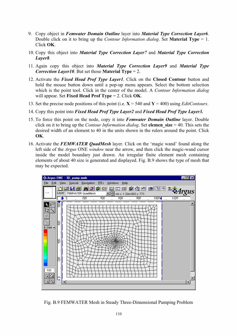
16. Activate the FEMWATER QuadMesh layer. Click on the ‘magic wand’ found along theleft side of the Argus ONE window near the arrow, and then click the magic-wand cursorinside the model boundary just drawn. An irregular finite element mesh containingelements of about 40 size is generated and displayed. Fig. B.9 shows the type of mesh thatmay be expected.

Fig. B.9 FEMWATER Mesh in Steady Three-Dimensional Pumping Problem

111

17. The band-width of a newly-generated mesh always needs to be reduced. Select theSpecial menu long the top of the Argus ONE window, then select Renumber.... Thisbrings up the Renumber window. In this window click on Optimize Bandwidth andthen OK. The mesh numbering is then optimized for the matrix solver currently used byFEMWATER-LHS.

18. Specify a constant elevation, or default elevation using the Layers dialog. In this case,enter 15, 30, 35, 40, 45, 50, 55, 60, 66, 72 in the Expression dialog for Nodal ElevationLayer2 through Nodal Elevation Layer11 respectively.

19. Specify a constant initial head, using the Layers dialog. In this case, enter 60, 45, 30, 25,20, 15, 10, 5, 0, -6, -12 in the Expression dialog for Initial Head Layer1 through InitialHead Layer11 respectively.

20. Save the project (e.g. to 3D_pump.mmb).


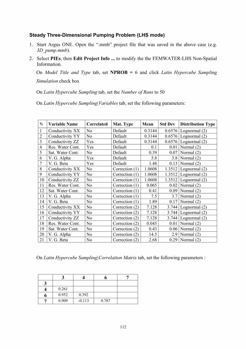
22. Using FEMWATER Post Processing in PIEs menu, plot pressure head for Three-Dimensional Surface Map type (Fig. B.10).

Fig. B.10 Head Surface Map in Steady Three-Dimensional Pumping Problem

112

Steady Three-Dimensional Pumping Problem (LHS mode)

1. Start Argus ONE. Open the “.mmb” project file that was saved in the above case (e.g.3D_pump.mmb).

2. Select PIEs, then Edit Project Info ... to modify the the FEMWATER-LHS Non-SpatialInformation.





N Variable Name Correlated Mat. Type Mean Std Dev Distribution Type

1 Conductivity XX No Default 0.3144 0.6576 Lognormal (2)2 Conductivity YY No Default 0.3144 0.6576 Lognormal (2)3 Conductivity ZZ Yes Default 0.3144 0.6576 Lognormal (2)4 Res. Water Cont. Yes Default 0.1 0.01 Normal (2)5 Sat. Water Cont. No Default 0.39 0.07 Normal (2)6 V. G. Alpha Yes Default 5.8 3.8 Normal (2)7 V. G. Beta Yes Default 1.48 0.13 Normal (2)8 Conductivity XX No Correction (1) 1.0608 1.3512 Lognormal (2)9 Conductivity YY No Correction (1) 1.0608 1.3512 Lognormal (2)10 Conductivity ZZ No Correction (1) 1.0608 1.3512 Lognormal (2)11 Res. Water Cont. No Correction (1) 0.065 0.02 Normal (2)12 Sat. Water Cont. No Correction (1) 0.41 0.09 Normal (2)13 V. G. Alpha No Correction (1) 7.5 3.7 Normal (2)14 V. G. Beta No Correction (1) 1.89 0.17 Normal (2)15 Conductivity XX No Correction (2) 7.128 3.744 Lognormal (2)16 Conductivity YY No Correction (2) 7.128 3.744 Lognormal (2)17 Conductivity ZZ No Correction (2) 7.128 3.744 Lognormal (2)18 Res. Water Cont. No Correction (2) 0.045 0.01 Normal (2)19 Sat. Water Cont. No Correction (2) 0.43 0.06 Normal (2)20 V. G. Alpha No Correction (2) 14.5 2.9 Normal (2)21 V. G. Beta No Correction (2) 2.68 0.29 Normal (2)

On Latin Hypercube Sampling|Correlation Matrix tab, set the following parameters :

3 4 6 734 0.261

6 0.952 0.392

7 0.909 -0.113 0.787

113

Then click OK.

3. Save the project (e.g. to 3D_pump_LHS.mmb).



Seawater Intrusion in Confined Aquifer

1. Start Argus ONE. In the FEMWATER-LHS Type of Simulation Problem window, select a

CROSS-SECTIONAL orientation. Then click Continue.

2. In the FEMWATER-LHS dialog, a number of changes to the initial default values are

required.

On Model Title and Type tab, set NPROB = 7

On Time Control tab, set:

NTI = 15

TMAX = 5000.75

DELT = 5

CHNG = 1.17169

DELMAX = 500

On Fluid Properties tab, set the coefficients for computing density and viscosity:

coeff. A1 Coeff. A2 coeff. A3 coeff. A4 coeff. A5 coeff. A6 coeff. A7 coeff. A81.0 0.0245 0.0 0.0 1.0 0.0 0.0 0.0

On Material and Soil Properties tab, click Material type correction check box to add the

correction material. Set the following parameters:

On Cond/Perm tab, set

xx yy zz xy xz yz1.0 0.0 1.0 0.0 0.0 0.0

On Soil Prop tab, set

Res MC Sat MC P Head VG Alpha VG Beta

0.1 0.35 0.0 5.8 1.48

On Disp/Diff tab, set

Dist coeff. Bulkdensity

Longdisper.

Transdisper.

Mol diffcoeff.

Turtuosity Decay const. Fr N/LangSMAX

0.0 1200 0.0 0.0 0.066. 1.0 0.0 0.0


N xx yy zz xy xz yz1 0.5 0.0 0.5 0.0 0.0 0.0

114


N Res MC Sat MC P Head VG Alpha VG Beta1 0.1 0.22 0.0 5.8 1.48

On Correction Disp/Diff tab, set

N Distcoeff.

Bulkdensity

Longdisper.

Transdisper.

Mol diffcoeff.

Turtuosity Decayconst.

Fr N/LangSMAX

1 0.0 1200 0.0 0.0 0.033. 1.0 0.0 0.0

On the Boundary Conditions|Dirichlet|Fixed Head tab, click Fixed Head check box and

then click Add Rows button to add the number of profile. Set the profiles as follows:

N Time 1 Head 1 Time 2 Head 21 0.0 100.49 1.0e38 100.492 0.0 100.735 1.0e38 100.7353 0.0 100.98 1.0e38 100.984 0.0 101.225 1.0e38 101.2255 0.0 101.47 1.0e38 101.476 0.0 101.715 1.0e38 101.7157 0.0 101.96 1.0e38 101.968 0.0 102.205 1.0e38 102.2059 0.0 102.45 1.0e38 102.45

On the Boundary Conditions|Dirichlet|Precribed-Concentration tab, click Prescr-

Concentration and set the profile:

N Time 1 Conctr 1 Time 2 Conctr 21 0.0 1.0 1.0e38 1.0

On the Boundary Conditions|Cauchy|Specified-Flux tab, click Specified-Flux and set the

profile:

N Time 1 S-flux 1 Time 2 S-flux 21 0.0 -6.6e-3 1.0e38 -6.6e-3

On the Boundary Conditions|Cauchy|Concentration tab, click Concentration and set the

profile:


On the Boundary Conditions|Variable Composite|Rainfall/Evap.-Seepage tab, click

Rainfall/Evap.-Seepage and set the profile:

N Time 1 Rf/Evap 1 Time 2 Rf/Evap 21 0.0 0.0 1.0e38 0.0

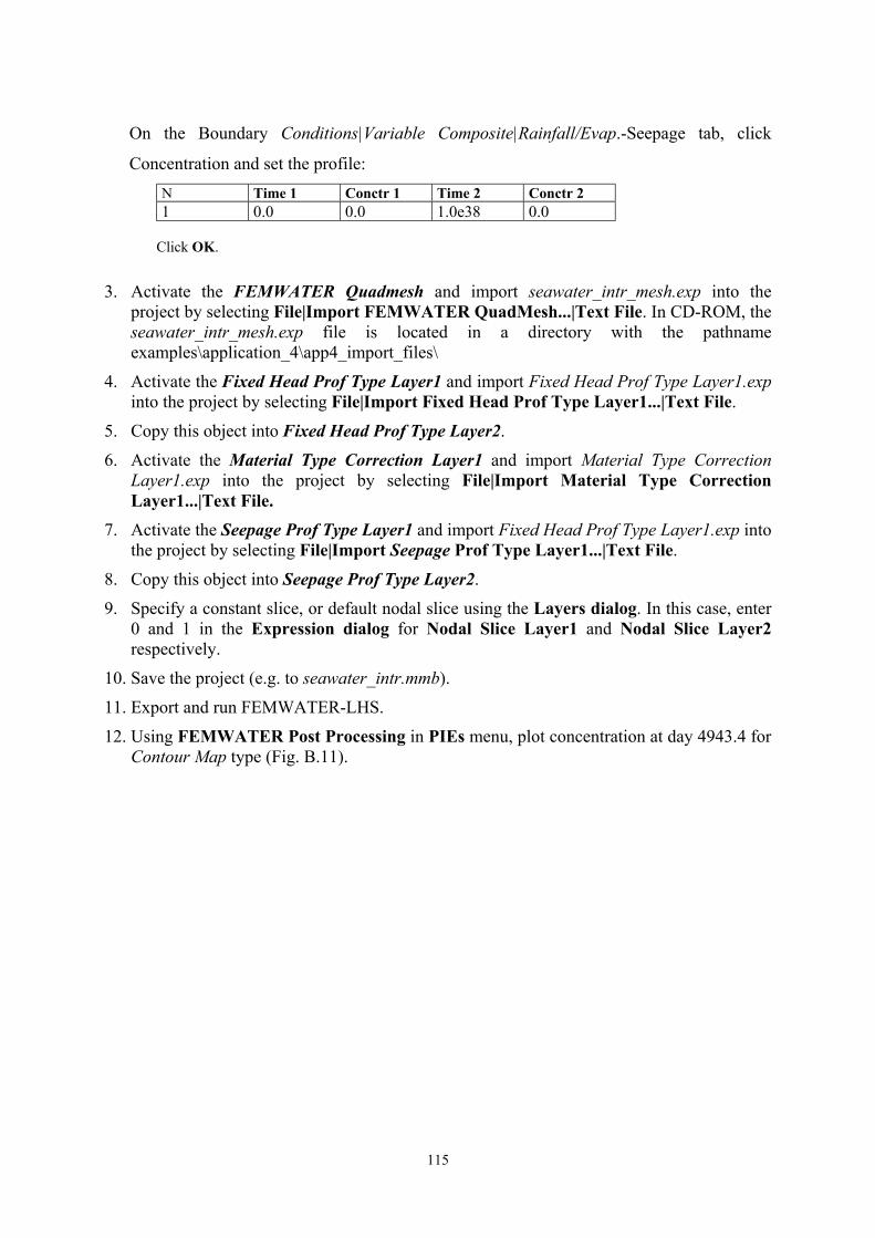
115

On the Boundary Conditions|Variable Composite|Rainfall/Evap.-Seepage tab, click

Concentration and set the profile:


Click OK.

3. Activate the FEMWATER Quadmesh and import seawater_intr_mesh.exp into theproject by selecting File|Import FEMWATER QuadMesh...|Text File. In CD-ROM, theseawater_intr_mesh.exp file is located in a directory with the pathnameexamples\application_4\app4_import_files\

4. Activate the Fixed Head Prof Type Layer1 and import Fixed Head Prof Type Layer1.expinto the project by selecting File|Import Fixed Head Prof Type Layer1...|Text File.

5. Copy this object into Fixed Head Prof Type Layer2.

6. Activate the Material Type Correction Layer1 and import Material Type CorrectionLayer1.exp into the project by selecting File|Import Material Type CorrectionLayer1...|Text File.

7. Activate the Seepage Prof Type Layer1 and import Fixed Head Prof Type Layer1.exp intothe project by selecting File|Import Seepage Prof Type Layer1...|Text File.

8. Copy this object into Seepage Prof Type Layer2.

9. Specify a constant slice, or default nodal slice using the Layers dialog. In this case, enter0 and 1 in the Expression dialog for Nodal Slice Layer1 and Nodal Slice Layer2respectively.

10. Save the project (e.g. to seawater_intr.mmb).


12. Using FEMWATER Post Processing in PIEs menu, plot concentration at day 4943.4 forContour Map type (Fig. B.11).

116

Seawater Intrusion in Confined Aquifer (LHS Mode)

1. Start Argus ONE. Open the “.mmb” project file that was saved in the above case (e.g.seawater_intr.mmb

2. Select PIEs, then Edit Project Info ... to modify the FEMWATER-LHS Non-SpatialInformation.





Fig. B.11 The concentration contours at the simulation time of 4943.4 days.

117

N Variable Name Correlated Mat. Type Min Max Distribution Type

1 Conductivity XX No Default 0.8 1.1 Lognormal (1)2 Conductivity ZZ No Default 0.8 1.1 Lognormal (1)3 Sat. Water Cont. No Default 0.315 0.385 Normal (1)4 Bulk density No Default 1080 1320 Normal (1)5 Mol diff coeff. No Default 0.0594 0.0726 Normal (1)6 Conductivity XX No Correction (1) 0.45 0.55 Lognormal (1)7 Conductivity ZZ No Correction (1) 0.45 0.55 Lognormal (1)8 Sat. Water Cont. No Correction (1) 0.198 0.22 Normal (1)9 Bulk density No Correction (2) 1080 1320 Normal (1)10 Mol diff coeff. No Correction (2) 0.0297 0.0363 Normal (1)

Then click OK.

3. Save the project (e.g. to seawater_intr _LHS.mmb).



appendix b step-by-step applications of the...

Documents