APPENDIX B: ENGINEER’S MANUAL

RSAP Version 3.0.0

N C H R P 22-27

ROADSIDE SAFETY ANALYSIS PROGRAM (RSAP) UPDATE

RoadSafe LLC 12 Main Street

Canton, Maine 04221

October 25, 2012

B-1

Table of Contents List of Figures ................................................................................................................................. 3

List of Tables .................................................................................................................................. 5

Introduction ..................................................................................................................................... 7

Background ..................................................................................................................................... 7

Overview ......................................................................................................................................... 8

Program implementation ........................................................................................................... 10

Data Input and Homogeneous Segments .................................................................................. 10

Encroachment Probabilty Module ................................................................................................ 11

Data analysis ............................................................................................................................. 12

Cooper Encroachment Data .................................................................................................. 12

Statistical Model and Estimation .......................................................................................... 15

Two-Lane Undivided Highway Analysis ............................................................................. 18

Four-Lane Divided Highway Analysis ................................................................................. 23

Comparison of Results .............................................................................................................. 26

Encroachment Frequency .......................................................................................................... 27

Multilane Adjustment Factor ................................................................................................ 30

Posted Speed Limit Adjustment Factor ................................................................................ 33

Access Density Adjustment Factor ....................................................................................... 34

Terrain Adjustment Factor .................................................................................................... 35

Vertical Grade Adjustment Factor ........................................................................................ 35

Horizontal Curve Adjustment Factor .................................................................................... 36

Lane Width Adjustment Factor ............................................................................................. 40

Adding New Encroachment Data and Adjustment Factors .................................................. 42

Vehicle Types ........................................................................................................................... 43

Vehicle Classifications.......................................................................................................... 43

Passenger Cars ...................................................................................................................... 46

Pickup Trucks, Vans and Sport Utility Vehicles .................................................................. 46

Buses ..................................................................................................................................... 47

Two-Axle Single Unit Truck ................................................................................................ 47

Five-Axle Tractor-Semitrailer Vehicle ................................................................................. 48

Combined Vehicle Categories .............................................................................................. 52

Adding New Vehicle Types .................................................................................................. 52

Crash Prediction Module .............................................................................................................. 53

B-2

Trajectory Look Up Table ........................................................................................................ 55

Trajectory Selection .................................................................................................................. 59

Trajectory Selection Methodology ....................................................................................... 60

Terrain Rollover ........................................................................................................................ 71

Rollover Model ..................................................................................................................... 76

Summary ............................................................................................................................... 78

Hazard Penetration .................................................................................................................... 79

Structural Penetration of Hazards ......................................................................................... 80

Roll-Over-Hazard Penetrations ............................................................................................. 94

Redirection .............................................................................................................................. 113

Factors Influencing Redirection Path .................................................................................. 113

RSAPv3 Implementation .................................................................................................... 119

Computing TRAJECTORY EFCCR ...................................................................................... 122

Example: Computing EFCCR for an encroachment path ................................................... 123

Severity Prediction Module ........................................................................................................ 127

Background ............................................................................................................................. 127

Speed and Crash Severity ................................................................................................... 128

Crash Severity Model ............................................................................................................. 131

Measure of Crash Severity .................................................................................................. 132

Penetration of Hazards and Impact-Side Rollovers ............................................................ 142

Summary of Results ................................................................................................................ 143

Adding New Hazards .......................................................................................................... 150

Benefit/Cost Module ................................................................................................................... 150

Project Costs ........................................................................................................................... 151

Crash Costs ............................................................................................................................. 152

Comprehensive Crash Costs ............................................................................................... 154

Background ......................................................................................................................... 155

Heavy Vehicle and Motor Cycle Adjustments ................................................................... 156

Summary ............................................................................................................................. 158

Benefit-COST RAtio Calculations ......................................................................................... 158

Validation .................................................................................................................................... 160

Lognormal Distribution .......................................................................................................... 161

Weibull Distribution ............................................................................................................... 161

Gamma Distribution ................................................................................................................ 162

B-3

Concrete Median Barrier Example ......................................................................................... 162

Cable Median Barrier .............................................................................................................. 165

Summary ................................................................................................................................. 170

Conclusions ................................................................................................................................. 170

References ................................................................................................................................... 171

LIST OF FIGURES Figure 1. Encroachment rate on one right-side edge by bi-directional AADT. ........................... 26 Figure 2. Possible Encroachments for Divided and Undivided Highways. ................................. 28 Figure 3. Comparison of Horizontal Curve Adjustment Factors. ................................................ 38 Figure 4. Horizontal Curve Adjustment Factors with HSM Symmetry Assumed. ..................... 38 Figure 5. HSM Horizontal Curve Adjustment Factor. ................................................................. 39 Figure 6. HSM Horizontal Curve Adjustment Factor. ................................................................. 40 Figure 7. HSM Lane Width Adjustment Factor. [AASHTO10] .................................................. 41 Figure 8: Vehicle properties for bus test vehicle in test 7069-7 [Buth97] .................................... 47 Figure 9: Two-axle SUT test Vehicle properties for test 476460-1b [Bullard10] ........................ 48 Figure 10: Illustration of collision sequence in tractor-semitrailer impacts with longitudinal

barriers (Test TL5CMB-2)[Rosenbaugh07] ......................................................... 49 Figure 11: Vehicle properties for tractor-van-trailer test vehicle used in Test TL5CMB-2 ......... 51 Figure 12. RSAPv3 Crash Prediction Module Flow Chart. ......................................................... 55 Figure 13: Cumulative distribution chart showing percent of crash cases with longitudinal and

lateral trajectories exceeding given values ........................................................... 58 Figure 14. Comparison of cross-section pairs and corresponding similarity scores.................... 62 Figure 15. Plots for horizontal curve radii corresponding to scores of 1.0, 0.93, 0.85 and 0.8

relative to a given horizontal curve radius of 1,910 feet. ...................................... 64 Figure 16. Plots for horizontal curve radii corresponding to scores of 1.0, 0.93, 0.85 and 0.8

relative to a given horizontal curve radius of 955 feet. ......................................... 64 Figure 17. Plots for horizontal curve radii corresponding to scores of 1.0, 0.93, 0.85 and 0.8

relative to a given horizontal curve radius of 637 feet. ......................................... 64 Figure 18. Tabulated and plotted score values for vertical grade as a function of the absolute

difference in percent grade. ................................................................................... 66 Figure 19. Plots of the roadside x-sections from the selected trajectory cases (dashed blue line)

compared with the Example Project x-section (solid red line). ............................ 69 Figure 20. Plots of the roadside x-sections from the selected trajectory cases (dashed blue line)

compared with the Example Project x-section (solid red line) continued. ........... 70 Figure 21. Probability of rollover as a function of sideslope from the NCHRP 17-11 study.

[Bligh04] ............................................................................................................... 72 Figure 22. Probability of rollover using FHWA supplemental data compared to values from the

17-11 simulation study. ......................................................................................... 74 Figure 23. Probability of rollover model implemented in RSAv3 Rollover Adjustment Factors

for Various Roadway Characteristics. .................................................................. 74 Figure 24. Probability of rollover as a function of sideslope and horizontal curve radius

[Bligh04] ............................................................................................................... 75

B-4

Figure 25. Adjustment factor for baseline probability of rollover as a function of sideslope and horizontal curve radius. ......................................................................................... 75

Figure 26. Probability of rollover as a function of sideslope and vertical grade. [Bligh04] ........ 76 Figure 27. Adjustment factor for baseline probability of rollover as a function of sideslope and

vertical grade. ........................................................................................................ 76 Figure 28. Vehicle and barrier geometry for calculating the average impact force according to

Olson. [Mak94] ..................................................................................................... 82 Figure 29. Damage to a 32” concrete bridge railing in a crash with a single unit truck in Florida.

[Alberson04] ......................................................................................................... 84 Figure 30: Probability model for structural penetration of hazards in RSAPv3 ........................... 91 Figure 31. Summary of results for TTI test 0482-1 on the G4(2W) with 12.5-ft post

spacing.[Mak93] ................................................................................................... 93 Figure 32. Schematic drawing of vehicle impacting barrier. ........................................................ 98 Figure 33. Freebody diagram for Phase 3. ................................................................................. 103 Figure 34. Freebody diagram for analysis of truck rolling onto the barrier. .............................. 104 Figure 35. Full-scale crash tests illustrating engagement points of vehicle during redirection for

(a) 32-inch tall barriesr [Bullard, 2010] and (b) 36-inch tall barriers. [Sheikh , 2011] ................................................................................................................... 108

Figure 36. Crash test photos and summary of maximum roll angles.......................................... 111 Figure 37. Crash test photos and summary of maximum roll angles (continued). ..................... 112 Figure 38. Departure and redirection path from a crash case in the 17-22 crash reconstruction

database. .............................................................................................................. 114 Figure 39. Plot of redirection angle vs. impact angle for collisions with rigid barriers. ............ 115 Figure 40. Plot of redirection angle vs. impact angle for collisions with semi-rigid and flexible

barriers. ............................................................................................................... 115 Figure 41. Cumulative distribution of redirection angles for rigid barriers from 17-11 crash

reconstruction database (passenger vehicles only). ............................................ 116 Figure 42. Cumulative distribution of redirection angles for semi-rigid and flexible barriers from

17-11 crash reconstruction database (passenger vehicles only). ........................ 116 Figure 43. Cumulative distribution of redirection angles for passenger vehicles from full-scale

crash test series 7069. ......................................................................................... 119 Figure 44. Cumulative distribution of redirection angles for commercial vehicles from full-scale

crash test series 7069. ......................................................................................... 119 Figure 45. Example illustrating collision prediction process in RSAPv3 for a single

encroachment ...................................................................................................... 124 Figure 46: Flow chart of possible collisions resulting from the example trajectory in Figure 45

and their probability of occurrence. .................................................................... 126 Figure 47. SI-Method Predicted Crash Costs versus Observed Crash Costs of Utility Pole

Crashes in Washington State and Maine. ........................................................... 130 Figure 48. EFCCR of Utility Pole and Tree Crashes in Washington and Maine as a Function of

Posted Speed Limit. ............................................................................................ 141 Figure 49. Observed and RSAP predicted crash costs for a 27-ft wide median with TL5 concrete

median barriers. ................................................................................................... 163 Figure 50. Observed and RSAP predicted crash costs for a 40-ft wide unprotected 6:1 median.

............................................................................................................................. 168

B-5

Figure 51. Observed and RSAP predicted crash costs for a 40-ft wide 6:1 median with a low-tension cable median barrier 8-ft from one edge of lane. ................................... 168

LIST OF TABLES Table 1. RSAPv3 Default Highway Characteristics. ................................................................... 11 Table 2. Two- and Three-Lane Undivided Highway Summary Statistics. .................................. 19 Table 3. Estimated Parameters and Statistics of Two-Lane Undivided Highways ..................... 21 Table 4. Four-Lane Divided Highway Summary Statistics. ........................................................ 23 Table 5. Estimated Parameters and Statistics of 4-Lane Divided Highways. .............................. 24 Table 6. Total Encroachment Frequency by AADT and Highway Type. ................................... 29 Table 7. Summary of 1998-99 Median Crashes from 52 Texas Counties. .................................. 30 Table 8. Summary Statistics of Sampled Road Sections ............................................................. 31 Table 9. Default Multilane Adjustment Look Up Table. ............................................................. 33 Table 10. Posted Speed Limit Adjustment Look Up Table. ........................................................ 34 Table 11. Default Access Density Adjustment Look Up Table. .................................................. 34 Table 12. Default Terrain Look Up Table. .................................................................................. 35 Table 13. Wright and Robertson Grade Look Up Table. ............................................................. 35 Table 14. Miaou Grade Look Up Table. ...................................................................................... 36 Table 15. Default Lane Width Adjustment Look Up Table. ....................................................... 41 Table 16. Maryland 2008 Vehicle Distribution by Vehicle Class ................................................ 45 Table 17: Recommended vehicle properties for use in RSAPv3 based on the 13 FHWA vehicle

classes ................................................................................................................... 46 Table 18. Default RSAPv3 Vehicle Properties Table .................................................................. 52 Table 19. Results of the trajectory selection process for the example case. ................................. 71 Table 20. 1991 FHWA Supplemental Information for use with the Roadside Program.

[FHWA91] ............................................................................................................ 73 Table 21. Bridge railing capacity recommendations in BCAP and NCHRP 22-08.[after Mak94]

............................................................................................................................... 84 Table 22. Performance of cable median barriers in various States. [Ray09, MacDonald07] ....... 87 Table 23. Barrier Performance in Washington State. ................................................................. 88 Table 24. Strengths and weakness of the mechanistic and statistical approaches to hazard

penetration............................................................................................................. 89 Table 25. Comparison of maximum roll angle from theoretical calculations with full-scale test

results. ................................................................................................................. 109 Table 26. Summary of impact and exit conditions from test series 7069.[Buth97] ................... 118 Table 27. Example of computing EFCCR for an encroachment path ........................................ 124 Table 28. NCHRP 492 Generic Severity Distributions. ............................................................ 128 Table 29. Police-Reported Severity of Utility Pole Crashes in the States of Washington (2002-

2006) and Maine (1994-1998). ........................................................................... 133 Table 30. Summary of Unreported Crashes Percentages by Hazard Type. ............................... 135 Table 31. Police-Reported and Maintenance Reported Utility Pole Crashes in Texas (1976-

1979). (4)............................................................................................................. 137 Table 32. Estimate of Total Crashes for Utility Pole Crashes in the States of Washington (2002-

2006) and Maine (1994-1998) Assuming 12.2 percent of Cases Unreported. ... 137

B-6

Table 33. Estimate of Total Crashes for Utility Pole Crashes in the States of Washington (2002-2006) and Maine (1994-1998) based on the Minimum Likely Unreported Crash Rate. .................................................................................................................... 138

Table 34. 2009 Crash Costs and EFCCRs of Utility Pole Crashes in the States of Washington (2002-2006) and Maine (1994-1998) .................................................................. 140

Table 35. EFCCR65 of Selected Roadside Features and Collisions. .......................................... 144 Table 36. Default Hazard Severity Table. ................................................................................. 149 Table 37. Economic Costs (2000 Dollars) of Reported and Unreported Crashes. [Blincoe09] 153 Table 38. Recent Comprehensive Crash Costs. ......................................................................... 154 Table 39. Comprehensive Cost per Single Vehicle Crash and All Crashes in 2001

Dollars.[Council11] ............................................................................................ 155 Table 40. 2005&2008 Cost of All Truck Crashes by Injury Severity and per Victim. ............. 156 Table 41. Relative Crash Costs for Heavy Vehicles and Motorcycles. ..................................... 157 Table 42. Results of Heavy Vehicle and Motorcycle Adjustment Analysis. ............................. 158 Table 43. Example of incremental benefit-cost selection. ......................................................... 159 Table 44. Statistical properties of the concrete median barrier validation example. ................. 164 Table 45. Collisions by collision type for a concrete median barrier in a 27-ft wide median. .. 165 Table 46. Statistical properties of the cable median barrier validation example. ...................... 169 Table 47. Collisions by collision type for the cable median barrier validation example. ........ 170

B-7

INTRODUCTION The Roadside Safety Analysis Program (RSAP) is a computer program for performing benefit-cost analyses on roadside design alternatives. RSAP assists roadside designer is choosing between multiple detailed alternative roadside designs by estimating the expected crash costs and performing an incremental cost-benefit analysis of the alternatives. The original version of RSAP was developed under NCHRP Project 22-9(1) and distributed with the 2002 edition of the AASHTO Roadside Design Guide (RDG). [Mak03, AASHTO02] Subsequently, some additional improvements were made, bugs corrected and patches installed under NCHRP Project 22-9(2) [Mak03]. Finally, a third NCHRP project, 22-9(3) was initiated but never completed. NCHRP Project 22-27 was initiated with the following objectives:

Rewrite the software, Update the manuals, Improve the user interface, and Update the embedded default data tables. This project resulted in RSAP version 3.0.0 (RSAPv3). RSAPv3 and the research which

contributed to the software development are documented herein. This Manual is one of three reports which accompany this software, including a USER’S MANUAL and a PROGRAMMER’S MANUAL. The ENGINEER’S MANUAL contains extensive explanations of the analysis methods, the supporting research and data used by the software, background information, explanation of existing software and literature and the implementation of this software. Information is also provided for developing and including new severity models or adjustment factors into RSAPv3 based on local data or new research.

The USER’S MANUAL is a reference for program users of all experience levels focusing on how to use the software and access its features. It includes several example problems that illustrate how data should be set up and entered and provides results that can be used to check a user’s first runs. The PROGRAMMER’S MANUAL a resource for programmers needing to modify the code. It documents the program architecture, the data table specifications and algorithmic procedures. This Manual should be used for specific information regarding which models are used in the program, how the models are used, and the supporting research. This manual provides guidance on how to supplement the default data tables with regional data or new research.

BACKGROUND A key step in performing a benefit-cost analysis is to estimate the frequency, severity and

societal cost of roadside crashes for a particular roadside design where the design encompasses highway geometric features like the horizontal curvature and grade, roadside and median terrain such as cuts, fills and ditches and the type and location of roadside features like guardrails, utility poles and trees. Once the frequency and severity of crashes has been estimated, the cost can be found by mapping the frequency and severity into units of dollars given the average societal cost of each expected crash. A roadside design that results in a smaller societal cost is by definition a safer and better design. The benefit-cost procedures identify the best use of scare funds with the objective of maximizing safety while minimizing overall costs. If the reduction in crash costs over the design life of the improvement are greater than the annualized construction and maintenance costs of the improvement the design is cost-beneficial and should be considered for construction. On the other hand, if the reduction in crash costs is less than the construction/maintenance cost of the improvement the project probably is not worth pursuing.

B-8

Estimating the frequency and severity of crashes for a given roadside design can be challenging since much data is required and numerous calculations are involved. The following chapters and sections describe the methods and techniques used in RSAPv3 to estimate the frequency and severity of crashes that can be expected for a roadside design and how to calculate the benefit-cost ratios to evaluate the cost effectiveness of those designs.

OVERVIEW RSAPv3 uses a conditional encroachment-collision-severity approach to determine the

frequency, severity and societal cost of roadside crashes for each user-entered design alternative. These crash costs are then compared to the agency costs (i.e., construction and/or maintenance, etc.) of the proposed alternatives. An alternative which results in a reduction in crash costs greater than the agency costs of the improvement is considered a feasible project. The alternative with the highest benefit (i.e., reduction in crash costs) to agency costs ratio is the “best” alternative. An RSAPv3 analysis is composed of four major steps for assessing each alternative and is, therefore, structured into four modules:

Encroachment Probability Module, Crash Prediction Module, Severity Prediction Module, and Benefit/Cost Analysis Module.

The analysis technique used by RSAPv3 is based on a series of conditional probabilities. First, RSAPv3 predicts the number of encroachments that can be expected on a given road segment as a function of the traffic and geometric characteristics of the roadway. Given an encroachment has occurred, the crash prediction module then assesses if the encroachment is likely to result in a crash, P(Cr|Encr). If a crash is predicted, the severity prediction module estimates the severity of the crash, P(Sev|Cr). The severity estimates of each crash are then calculated and transformed into units of dollars in order to compare the reduction in societal crash costs (i.e., benefits) to the direct cost of implementing the alternative (i.e., costs). The following conditional probability model is used for each alternative on each segment:

E(CC)N,M = ADT · LN · P(Encr) ∙P(Cr|Encr) ∙ P(Sev|Cr) ∙ E(CCs|Sevs)

where: E(CC)N,M = Expected annual crash cost on segment N for alternative M, ADT = Average Daily Traffic in vehicles/day, LN = Length of segment N in miles, P(Encr) = The probability a vehicle will encroachment on the segment, P(Cr|Encr) = The probability a crash will occur on the segment given that an

encroachment has occurred, P(Sevs|Cr) = The probability that a crash of severity s occurs given that a crash has

occurred and E(CCs|Sevs) = The expected crash cost of a crash of severity s in dollars. The term ADT·L·P(Encr) yields the expected number of encroachments on a segment in units of encroachments/mi/year. ADT·P(Encr) can be further defined as:

B-9

∙ ∙

where the terms are as defined before, fbase encr is the base encroachment rate in units of encroachments/mi/yr and EAFi are encroachment adjustment factors. fbase encr is tabulated on the “Encr Freq and Adj” worksheet in RSAPv3 as are the encroachment adjustment factors, EAFi. These values are simple lookup tables where the appropriate adjustment or base encroachment is read from the tables given the geometric and traffic characteristics of the highway provided by the user. The collision and severity conditional encroachments, P(Cr|Encr) ∙ P(Sevs|Cr), must be grouped together because each encroachment could have multiple events with different severities. P(Cr|Encr) ∙ P(Sevs|Cr) can be expanded to:

| |1

∩ | | ∩

Where ∩ is the probability that trajectory k will intersect hazard j and the summation is done over all hazards (i.e., hazards k=1 to l where l is the maximum number of hazards), and all trajectories (i.e., for trajectories j=1 to m where m is the maximum number of trajectories). RSAPv3 will typically process tens of thousands of trajectories for each segment to arrive at this summation. Each trajectory analyzed is compared to every hazard identified by the user for each alternative. Lastly the expected crash cost of a severity s crash, E(CCs|Sevs), is multiplied by the result to convert the result to units of dollars. Combining all the terms yields:

, ∙

1

∩ ∩ |

While the encroachment method is conceptually straight forward, estimating the three conditional probabilities at the heart of the method can be difficult and computationally demanding since tens of thousands of possible encroachments must be evaluated. Each of these conditional probabilities is based either on observed encroachment or crash data. Since the computations can be complicated, a computer program like RSAPv3 is the most convenient way to implement the encroachment-based approach in roadside safety analysis. Each of these condition probabilities is implemented within RSAPv3 as a module. The results of the analysis (i.e., E(CC)N,M) are used in the benefit/cost module to compare roadside design alternatives. Project specific data is collected from the user through a series of worksheets within the RSAPv3 user interface. This project specific data is used in conjunction with models based on research stored in other worksheets to preform calculations which are coded in RSAPv3. Unlike earlier versions of RSAP, RSAPv3 does not use a Monte Carlo simulation method to calculate the probability of a collision given an encroachment. Instead, a deterministic method is used where a sample of real crash trajectories are compared to the roadside and used to perform the double summation in the equation above. The encroachment probability module, crash prediction module, severity prediction module, and the Benefit/Cost module are described in the following sections. Each chapter presents the research conducted under this project and discusses how the research was

B-10

implemented in the software. Each chapter contains background relevant to the subject heading. For example, the background presented in the severity prediction module chapter pertains to crash severity. This document mirrors the USER’S MANUAL and PROGRAMMER’S MANUAL to the extent possible. Each manual takes the same general form and references have been made to other manuals to avoid duplication across manuals.

PROGRAM IMPLEMENTATION RSAPv3 is written as a series of Visual Basic (VB) macros within Microsoft Excel. RSAPv3 uses the usual Excel worksheets as a means for collecting and organizing information about the road characteristics and the alternatives to be analyzed. RSAPv3 was developed primarily using Excel version 14 running under the Windows NT 6.01 operating system although it has been tested and works correctly for Excel 12 and Windows 2007 as well. The macros operate in the background through a special RSAP Controls Dialog box which allows users to progress through the stages of data entry, analysis and examining results. Each tab in the dialog provides the facilities to enter, change and modify the input values including the default values in RSAPv3. The worksheet in RSAPv3 are protected and some are hidden to prevent inadvertent data entry in incorrect locations from compromising the analysis. If new information needs to be added, there are instructions in this manual for unprotecting and un-hiding worksheets so that changes and modifications can be made. More information on the programming aspects of RSAPv3 are provided in the Programmer’s Manual.

DATA INPUT AND HOMOGENEOUS SEGMENTS RSAPv3 has much data stored within the program to support these calculations and

modeling, however, project specific data must be entered by the user for each project. The user must enter the highway geometrics, the roadside design alternatives, and the traffic characteristics. The encroachment probability module estimates the frequency of encroachments for each homogeneous highway segment. Previous versions of RSAP required the highway be manually segmented into homogeneous segments prior to data entry. RSAPv3 accepts highway characteristics in any order and automatically segments the highway into homogeneous segments for the user. Additionally, roadside hazard locations can be entered in any order, as RSAPv3 segments the highway and sorts the hazard data prior to the analysis. These features are described in the USER’S MANUAL.

After the user has entered all the road characteristics on the “Road Segments” worksheet and selected the “Segment Project” button on the RSAP Controls Dialog, RSAP scans through the list of characteristics and organizes them into homogeneous segments where all the characteristics are the same. It is not desirable to have unnecessarily short segments so sometimes it will work best to align the geometric and cross-section properties so they fall at the same station. For example, if a horizontal curve goes from Station 1+50 to 2+75 and there is a vertical grade from 1+45 to 2+80 RSAP would segment this into three segments: one five feet long, one 125 ft long and the last five feet long. RSAP will function even with these short segments but it would be easier to review and understand the results if, for example, both the horizontal curve and grade started and stopped at the same station.

The highway characteristics that are recognized by RSAPv3 are shown in Table 1 along with the default values by highway type. If a characteristic for a segment is not defined, RSAPv3 assumes the default value shown in Table 1 for the chosen highway type. For example, if the horizontal curve and grade are defined for a segment on an undivided highway but the lane

B-11

width is not, RSAPv3 will assume 12-ft lanes. The user, therefore, only needs to enter characteristics that differ from the default values.

Table 1. RSAPv3 Default Highway Characteristics.

Highway Characteristic Units

Highway Type

Divided Undivided OnewayPosted Speed Limit mi/hr 65 65 65 Terrain F / M / R F F F Total Number of Lanes 4 2 1 Primary Direction Grade % 0 0 0 Primary Direction Radius of Curve ft T T T Lanes in Primary Direction 2 1 1 Median Width ft 30 Median Shoulder Width ft 10 Lane Width ft 12 12 12 Access Density points/mi 0 0 0 Rumble Strips true/false FALSE FALSE FALSE Right Shoulder Width ft 6 6 6

ENCROACHMENT PROBABILTY MODULE RSVPv3 is based on a theory of how crashes occur. Events are divided into a series of conditional events and each event is modeled. These conditional events include: the encroachment probability, the probability of crash given an encroachment, the severity of the crash if an object is struck and the cost of the entire crash sequence. The probability of an encroachment (i.e., vehicle leaving the road) has been the focus of many studies in the last forty years, however very little successful data collection on the frequency of encroachments has been accomplished. Data collected by Cooper and by Hutchinson and Kennedy have received much attention, but there are few alternate sources of encroachment data. [Cooper82; Hutchinson62] RSAPv3 uses the Cooper data but the data was re-analyzed to attempt to resolve some long-standing problems with the data.

The results of the re-analysis included generating baseline encroachment frequencies for two-lane undivided, four-lane and multi-lane divided highways. The base conditions for the encroachment frequencies are:

Posted speed limit of 65 mph, Flat ground, Relatively straight segment, Lane width greater than or equal to twelve feet, and Zero major access points per mile. Deviating from these base conditions requires the use of adjustment factors to calibrate

the encroachment frequency to the specific site conditions. RSAPv3 includes many more adjustment factors then the previous versions of RSAP. [Mak03] Some of these adjustment factors have only a few data points, while others are more complicated. This chapter provides

B-12

descriptions of the data and statistical methods used to estimate encroachment frequencies. This chapter also discusses how the base encroachment frequencies differ from those previously derived from the Cooper data and the use of adjustment factors to modify the base encroachment frequencies for specific segments. The estimates from these analyses have been provided as default values in RSAPv3, in the absence of local data. In the event local encroachment data are available, tables which match the formats shown below for the encroachment frequency and accompanying adjustment factors can be created and added to RSAPv3 as will be discussed at the end of the section.

DATA ANALYSIS Default values for the base encroachment frequency tables and adjustment LUTs have

been provided in RSAPv3. The data collection and preparation efforts to develop the default values using the Cooper data are presented here. The variables used by this project are discussed, including their definitions and characteristics. Instructions for changing the default values are provided at the end of this section.

Cooper Encroachment Data The data collection efforts and supplemental office data linkage with roadway and

environmental characteristics for the Copper were documented in multiple reports. [DeLeuw78; Cooper80; Cooper81] Twelve data collection teams were recruited and trained in June of 1978. Field collection took place during a four-month period from July to October in 1978. Over the period, tire-tracks generated and objects struck by vehicles on roadside were monitored, marked, measured, and graphed, to count and characterize vehicle encroachments. According to the field report, the field crew was mindful that some tire-tracks might be generated by vehicles performing highway and railroad maintenance work and efforts were made to exclude those encroachments. The data were collected on 59 road sections, each between 60 and 100 km in length. The road sections were selected from 5 geographically dispersed Canadian provinces. The study sections were not homogeneous in key attributes, including the posted speed limit, annual average daily traffic (AADT), and paved shoulder width. The posted speed limits of subsections ranged from 70 to 100 km/hr.

The field report provides an account of the planning, operation, and execution of the data collection efforts and documents experience gained throughout the collection process. It touches on several field data collection issues and discusses actions taken when problems were encountered. Overall, the report gives a glimpse of the nuances and potential issues that such a field data collection effort may experience.[DeLeuw78]

The efforts made and procedures used to supplement each field-collected encroachment case with the related traffic, roadway and roadside geometrics, and weather data were reported by Cooper.[Cooper80; Cooper81] These reports provided the rationale and procedures used to delineate long road sections into shorter road segments for developing encroachment rate models.

Captured and Missed Encroachments Each road section was surveyed within a one-day period at one-week intervals for the

duration of the study period. For two- and three-lane undivided highways, encroachments that encroached onto both edges of the undivided highways, including all four travel-directions and encroachment-side combinations, were collected. For four-lane divided highways, only those encroachments that to the right of the edge line of the thru lanes were collected (i.e.,

B-13

encroachments occurred in the median area were not collected). A small number of encroachments that crossed both the median and the opposite travel lanes were detected and included in the data set.

The encroachment data was based on monitoring tire-tracks and the field crew drove through each road section only about once a week; therefore, any encroachment that did not go beyond, or only slightly went beyond, the paved or graveled shoulders would be very difficult to detect for many obvious reasons. Recall that a vehicle roadside encroachment is defined as a vehicle inadvertently traveling beyond the edgeline of a travelled-way, which includes vehicles which do not leave the shoulder. An operational definition of encroachments was adopted as being beyond the paved and graveled shoulder to allow the field crew to focus their attention on the area beyond the shoulder when they drove through study road sections.[Cooper80] In statistical term, this type of data is said to be “left-truncated.” The level of truncations (i.e., the extent of missed encroachments that never left the shoulder) increases as shoulder width of the highways increases.

The encroachment rate is expected to be higher under inclement weather conditions for any road segment. More specifically, under wet, slippery road surface condition or limited sight distance visibility, a higher proportion of drivers are expected to lose traction or control of their vehicles and run off the road. Since the field collection of Cooper data took place only during the summer months, it is expected that the number of weather-induced encroachments in the Cooper data set would be under-represented when the data are expanded to represent the encroachments for the whole year. In short, annual encroachment rates generated from the Cooper data are expected to be lower than the true encroachment rates because of the temporal constraint of the field collection.

Despite the due diligence carried out by the field crews, some encroachments were inevitably missed. The field report shows evidence that field crews were trying to spot as many encroachments as possible while driving the study sections. Capturing 90% of the encroachments appeared to be the goal. For example, one of the team reported that “To ensure that 90% of the off road accidents are being found the van should travel along the shoulder at a speed no greater than 50 kilometers per hour and that the team members should change positions every 20 kilometers.”[DeLeuw78]

Truncated and Censored Encroachment Measurements The survey targeted the following three parameters for each detected encroachment:

Maximum extent of lateral encroachment: perpendicular distance measured from the edgeline of the rightmost thru lane to the farthest point of lateral departure or the point where the first fixed object is struck

Longitudinal distance: parallel distance along roadway from the first point where the vehicle leaves the edge of the thru lane to the point where the maximum extent of lateral encroachment occurs

Encroachment angle: angle of departure measured from the tangent to the edgeline of the travelway at the estimated point of departure (POD) to the line connecting the tire-track path, at the point where the vehicle first leaves “the shoulder” and the estimated POD. In statistical terms the distance data are left truncated in that only those encroachments

that traveled beyond shoulders were recorded (with very few exceptions), and the level of truncation varies from site to site as shoulder width varies. The distance data are also “interval censored” in that for each encroachment case the location of the maximum lateral distance is

B-14

given in the form of a 2m by 2m grid. That is, the extent of lateral encroachment can only be known to occur within a 2m by 2m squared grid, but the exact location within the grid is unknown from the data.

Further complicating the analysis, the data are “right-censored” in two different ways: About 37% of the encroachments struck fixed objects and the lateral distances

were measured from the edgeline to the first fixed object struck. For these encroachment cases, the distance is right-censored in that if the roadside were free of objects the extent of lateral encroachment would have been longer than the distance recorded.

When the lateral distance of encroachments exceeded a certain distance, the same code representing a catch-all-beyond distance category was recorded. The same coding scheme was used for longitudinal distances. Specifically, lateral distances beyond 16m, e.g., 21m and 40m, were all recorded as occurring in the 16m to 18m interval, which was the last interval allowed for recording the lateral distance; and longitudinal distances beyond 196m, e.g., 200m and 300m, were all recorded as occurring in the 196m to 198m interval, the last interval allowed for recording the longitudinal distance. About 9.3% of the encroachments have maximum lateral distance greater than 16m, and less than 1% of cases with associated longitudinal distances beyond 196m.

To summarize, the encroachment distance data in Cooper are left-truncated for almost all encroachments, and depending on whether an encroached vehicle struck fixed objects and the distances traveled, they are either right-censored or interval-censored. Statistical techniques to handle this type of data have been researched vigorously in the biomedical science and reliability engineering fields in the last three decades. It is well-known that if the truncation and censoring natures of the data are not properly formulated into the statistical estimation procedure, the modeling results are likely to be biased (e.g., Klein and Moeschberger, 2003). This is especially true for the Cooper distance data, where almost all data are left-truncated and a significant portion of the data are right-censored.

Road Segments Out of the 756 road segments, 575 segments were two- or three-lane undivided highways

and 181 segments were four-lane divided highways. A total of 1,881 encroachments occurred on these segments. Most of the attributes considered are not homogeneous within a segment. For example, the general descriptors for highway alignments provided in the file indicate average alignment characteristics over the whole segment.

The two- or three-lane undivided highway segments, the length-weighted posted speed limit varies from 72.5 to 97.5 km/hr excluding those segments with missing values, with close to 60 percent of the segments under 80 km/hr. The four-lane divided highways vary from 77.5 to 97.5 km/hr, with over 76 percent of the segments over 90 km/hr.

The study road segments range in traffic volumes from about 1,000 to 13,000 vehicles per day for the two- and three-lane undivided highways and 6,000 to 45,000 vehicles per day for the four-lane divided highways.

Cooper used the exploratory statistical “clustering” technique to delineated 54 of the study road sections to create a road segment file that contains 756 road segments for estimating encroachment rates. Cooper provided two main reasons for the need to delineate “sections” into shorter “segments”: (a) to increase the number of “data points” (or sample size), which would be beneficial statistically, and (b) to reduce the diluted effects of mixing various geometric features

B-15

in these relatively long sections. For these reasons, Cooper stated “It was thus considered necessary to subdivide the sections, and the means in which this is done is perhaps the most critical stage in the data reduction process.”[Cooper80] The clustering techniques basically grouped “similar sites” within a section to form segments based on a subjective “similarity” measure. Cooper adopted a “similarity” measure that was based primarily on the spacing between encroachment cases and secondarily on traffic volume. In other words, within a section, sites with encroachment cases that were closer in space, and perhaps similar in traffic volume, were grouped to create segments.

This so-called “data reduction” procedure performed by Cooper using the clustering techniques created a statistically flawed segment data file. This procedure made the determination of analysis units (i.e., road segments) dependent on the outcome variable (i.e., encroachments). This dependency introduced some bias into the segment data. More specifically, it artificially inflated the highs and deflated the lows of encroachment frequencies among the delineated road segments. The consequence is that any relationship developed from the segment data regarding the encroachment frequency or rate are likely to be overstated. In summary, the relationships indicated by any encroachment rate model developed from the Cooper segment data are likely to be overstated, and should be used with this limitation in mind.

Summary The data available in this project for analysis are contained in three electronic files: an

encroachment case file, a segment data file, and a section data file. The encroachment case file contains 1,949 records, each of which represents an individual encroachment case detected and investigated in the field. Each record contains variables that quantify the characteristics of the encroachment, such as encroachment angle, encroachment distances, objects struck, as well as those variables that describe the traffic, roadway, and roadside conditions of the site where the encroachment occurred. The road section file contains 37 records, providing identifiers and attributes for 37 of the 59 sections surveyed. The road segment file contains 1,512 records, including identifiers and variables for 756 road segments with one record per direction, which were delineated from 54 of the 59 surveyed sections. Five of the sections, all surveyed by one team (Team #9), were eliminated in preparing for the segment data due to questionable quality.

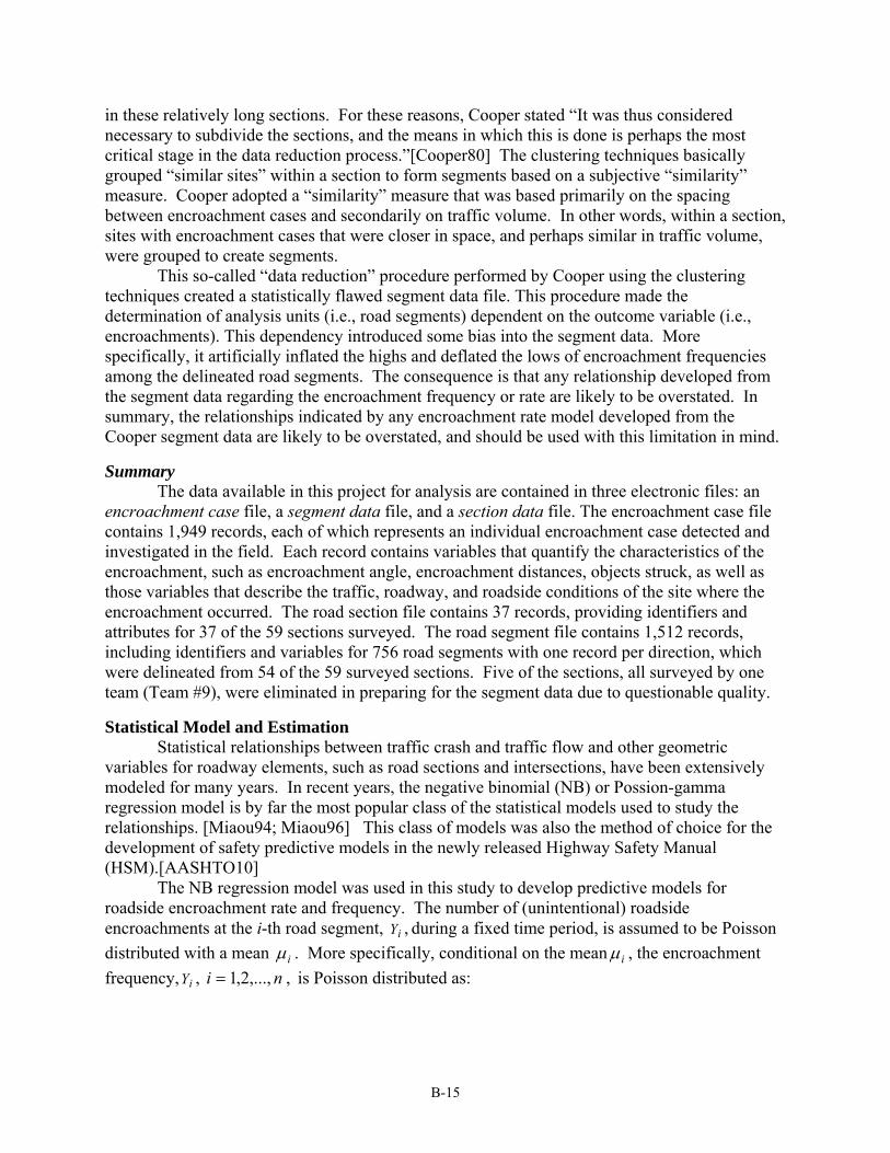
Statistical Model and Estimation Statistical relationships between traffic crash and traffic flow and other geometric

variables for roadway elements, such as road sections and intersections, have been extensively modeled for many years. In recent years, the negative binomial (NB) or Possion-gamma regression model is by far the most popular class of the statistical models used to study the relationships. [Miaou94; Miaou96] This class of models was also the method of choice for the development of safety predictive models in the newly released Highway Safety Manual (HSM).[AASHTO10]

The NB regression model was used in this study to develop predictive models for roadside encroachment rate and frequency. The number of (unintentional) roadside encroachments at the i-th road segment, iY , during a fixed time period, is assumed to be Poisson

distributed with a mean i . More specifically, conditional on the mean i , the encroachment

frequency, iY , ni ,...,2,1 , is Poisson distributed as:

B-16

)1.1(,...,,2,1!

)|( niwherey

eyYp

i

yi

iii

ii

It is also assumed that, given the mean i , iY , ni ,...,2,1 , are mutually independent among the

n road segments. For segment i , assume that the proportion of encroachments not detected, due to

limitations of the field data collection instrument, is a constant iu . This makes the “recorded” or

observed number of encroachments at the i-th road segment, iY~

, during a fixed time period, to be

Poisson distributed with a mean i~ , where )1(~iii u . Given the mean i and the

underreporting proportion iu , the recorded encroachment frequency, iY~

, ni ,...,2,1 , is Poisson

distributed as:

)2.1(,...,,2,1!~

~)~|~~

(~~

niwherey

eyYp

i

yi

iii

ii

Given i~ , iY~

, ni ,...,2,1 , are mutually independent.

The mean of the Poisson distribution, i , is assumed to vary from road segment to road

segment. In addition, the variation is a function of two sets of variables associated with these segments: (1) observed traffic and highway variables, and (2) unobserved, including unobservable, variables. More specifically, it is structured as:

)3.1()0

exp(1

i

eij

xji

vvJ

jiii

where the mean i is a multiplicative function of the amount of travel incurred iv and

encroachment rate i ; and i is an exponential function of the observed variables ijx ,

Jj ,...,2,1 , unobserved variable ie , and unknown regression parameters j , Jj ,...,2,1,0 .

The statistical literature usually calls iv an “offset,” representing total vehicle miles or

kilometers traveled on segment i during a period. Basically, iv quantifies the total amount of

vehicle exposures to (or total opportunities for) encroachment risks on the segment. For road segments, exposure measures are typically measured in units of million vehicle miles traveled (MVMT) or million vehicle kilometers traveled (MVKT).

The encroachment rate in number of encroachments per MVMT or MVKT is i and it is

a function of a set of covariates, such as those traffic and highway variables listed in Table 2, and an “error term” ie . The j-th covariate is symbolized as ijx , Jj ,...,2,1 . The regression

parameter (or coefficient) 0 is an unknown intercept term, and j , Jj ,...,2,1 , are unknown

regression parameters associated with the j-th covariates ijx .

In the Poisson-gamma model, the “error term” ie is assumed to be an unstructured

random effect independent of all available covariates ijx , Jj ,...,2,1 . In addition, exp( ie ) is

B-17

assumed to be independent and gamma distributed with mean equal to 1 and variance /1 for all segments ( > 0). This particular formulation provides flexible and attractive statistical

properties. For example, conditional on i and , iY can be shown to be distributed as a NB

random variable with mean and variance of i and /2ii , respectively. One useful way to

interpret the role of the “error term” is to view the variation of exp( ie ) across road segments as

un-modeled heterogeneities due to the variation of omitted exogenous variables across segments and the intrinsic randomness specific to each individual segment. For simplicity, omitted exogenous variables can be thought of as those variables that have effects on encroachment rates but are not available for modeling. The parameter is called the “inverse dispersion parameter” in that the Poisson model can be regarded as a limiting model of the NB as approaches infinity.

The proportion of encroachments not recorded for segment i due to limitations of the data collection instrument is iu . As presented above, encroachments with the extent of lateral

encroachment less than the paved and graveled shoulder width with very few exceptions were not recorded. In statistical term, the encroachment data are said to be “left-truncated.” The level of truncation increases as the shoulder width increases. In this analysis, the probability iu

is an estimate of the proportion of encroached vehicles that did not travel beyond the shoulder on segment i, given the width of the shoulder. It was estimated based on probability models developed using individual encroachment cases contained in the Cooper encroachment case file. Each record in the case file contains variables that quantify the characteristics of an encroachment, such as encroachment angle, encroachment distances, objects struck, as well as those variables that describe the traffic, roadway, and roadside conditions, under which the encroachment occurred.

Several encroachment distance models were tested statistically. The best model was a Weibull model with gamma random effects. This type of models is typically called “Weibull model with a shared gamma frailty distribution” in the biomedical science literature.[Duchateau08] A similar model was used to study the relationships between encroachment angles and highway, traffic, and vehicle variables. The model parameter estimation procedure was formulated to take into account of the unique characteristics of the Cooper encroachment distance data, including left-truncation, interval censoring, and right-censoring.[Klein03] Based on the developed lateral distance model, the probability iu was

estimated for each road segment in the Cooper segment file. On average, about 44 percent of the encroachments were estimated to be unrecorded for the two-and three-lane undivided road segments, and about 34 percent unrecorded for the four-lane divided segments.

In the development of both the encroachment rate and encroachment distance models, a full Bayesian approach was taken for model specification and estimation. One of the advantages of taking such an approach is that it takes full account of the uncertainty associated with the estimates of the model parameters and can provide exact measures of uncertainty. Non-informative priors were used for all the hyperparameters involved. For example, in specifying priors for the encroachment rate models, and were assumed to be mutually independent, with ’s having rather “flat” independent normal priors and having a rather diffused gamma prior distribution. This set-up of priors forces the estimation results from the Bayesian approach to be close to the results from the likelihood-based approach in the classical statistics. For the encroachment rate model, the maximum likelihood estimation (MLE) method was also used to

B-18

estimate the model parameters and, as expected, the results were almost identical to the results from the full Bayesian method.

Two-Lane Undivided Highway Analysis Default base encroachment frequencies from the Cooper data for two-lane undivided

highways were developed for inclusion in RSAPv3. Summary statistics of highway and traffic variables for two- and three-lane undivided highway segments are presented in Table 2. Many of these variables were selected for the final stage of model development.

There were a total of 1,353 encroachments observed during the field survey period for the 575 segments. The total vehicle kilometers during the period were 1,985 million vehicle kilometers traveled (MVKT). Thus the overall encroachment rate was 0.68 enc/MVKT (1.09 enc/MVMT). About 21.6% of the encroachments on two- and three-lane undivided highways were described as left-side departures, which means that the vehicle encroached on the centerline and then crossed the opposite travel lanes. The estimated base encroachment rate should be reduced by 21.6% to approximate the encroachment rate for right-side encroachments in the direction of travel.

B-19

Table 2. Two- and Three-Lane Undivided Highway Summary Statistics.

Variable Mean StdDev.

Min Max Total Distribution

Observed Number of Encroachments (including all 4 travel- direction and encroachment-side Combinations)

2.4 2.0 0 20 1,353 ------

AADT Segment Length (km) Exposure (MVKT) (=123*AADT*Segment length in km/1,000,000)

4,794 6.4 3.5

2,35510.86.4

1,0000.50.1

12,90380.065.4

------3,6981,985

------ ------ ------

Number of Lanes 2 Ln = 441 segments (76.7%)3 Ln = 134 segments (23.3%)

Posted Speed Limit (PSL) – Length-Weighted Average Speed (km/hr)

82.3 6.4 72.5 97.5 ------ 72.5—80 = 336 segments (58.4%) 80—90 = 184 segments (32%) 90—97.5 = 55 segments (9.6%)

Terrain Type (Based on Vertical Segment Geometry)

Flat = 163 segments (28.4%)Rolling = 305 segments (53%) Mountainous = 107 segments (18.6%)

Major Access-Point Density (Number of major road and highway Access Points/km)

1.2 1.5 0.002 9.4 ------ ------

Curve Severity Moderate-Long Radius = 495 segments (86%)Short-Moderate Radius = 40 segments (4%) Unknown = 40 segments (4%)

Horizontal Segment Geometry

Long Tangent + Curve = 398 segments (69%)Reverse Curve = 177 segments (31%)

Shoulder Width: Paved + Gravel (m) – Length-Weighted Average

2.9 0.8 0.2 6.2 ------ ------

Note: Overall encroachment rate = 1,353/1,985 = 0.68 ENCR/MVKT = 1.09 ENCR/MVMT, where MVKT = million vehicle kilometers traveled and MVMT = million vehicle miles traveled.

B-20

Modeling Results The mean encroachment rate for two-lane undivided highways can be expressed

mathematically as follows:

ENCR/MVKT = e(0.8528 – 0.3531·I(PSL>90) + 1.015·Rolling +0.8194·Mountian – 0.2805·3LN -0.2092·AADT/1000 +0.6393·AD) (1.4) Where:

ENCR/MVKT = encroachments per million vehicle kilometers traveled (MVKT) I(PSL>90)= 1 if posted speed limit > 90 km/hr; I(PSL>90) =0, otherwise Rolling = 1 if rolling terrain; Rolling =0, otherwise Mountain = 1 if mountainous terrain; Mountain = 0, otherwise 3Ln = 1 if 3-lane highways; 3Ln = 0 for 2-lane highways AADT = annual average daily traffic (AADT) in veh/day. AD = major access-point density in number of road and highway access points per km

The results of the encroachment rate model are presented in Table 3. It contains the mean

and standard error of the estimated model parameters and goodness-of-fit statistics of the model. Among the variables in the model, access density, AADT, and terrain type are the most statistically significant variables.

B-21

Table 3. Estimated Parameters and Statistics of Two-Lane Undivided Highways

Variable Estimated Coefficient

Offset = Exposure (in MVKT) = iv

( iv =365*AADT*Segment Length/1,000,000)

------

Intercept Term ( 0 ) 0.8528 (0.15)

Posted Speed Limit, PSL, (in km/hr): =1, if PSL > 90 ; =0,

otherwise ( 1 )

-0.3531 (0.19)

Rolling Terrain: =1 if Yes; =0, otherwise ( 2 ) 1.015 (0.12)

Mountainous Terrain: =1 if Yes; =0, otherwise ( 3 ) 0.8194 (0.18)

3-Lane: =1 if Yes; =0, otherwise ( 4 ) -0.2805 (0.14)

AADT ( 5 )

(in 1,000s of vehicles/day)

-0.2092 (0.02)

Major Access-Point Density ( 6 )

(in number of major road and highway access points per km)

0.6393 (0.04)

Inverse Dispersion Parameter

Inverse Dispersion Parameter ( ) 1.349 (0.11)

Inverse Dispersion Parameter for Model w/ Intercept

Term , 0 , Only ( 0 )

0.6741 (0.05)

Goodness-of-Fit Measures (Hilbe, 2011, Section 7.4)

)/1/()/1(1 02 MR 0.50

Notes: (1) Parameters ( s' and ) were estimated using Markov chain Monte Carlo (MCMC) techniques

and the values shown in the table are their posterior means, and (2) Values in parentheses are the estimated standard error of parameters based on the posterior density of the parameter.

Base Encroachment Rates Given the variables included in Eq. (1.4), the following explicit base conditions were chosen: Number of lanes: 2 Lanes (i.e., 3Ln = 0) Posted speed limit: 65 mph or 104 km/hr (i.e., I(PSL>90)=1) Terrain: Level (i.e., Rolling =0 and Mountain=0) Access Density: No major intersecting roads or highways (i.e., AD = 0)

Considering the conditions under which the data were collected and those variables that were

not found to be statistically significant, implicit base conditions should include good weather, good pavement conditions, lane width of about 12 ft (3.6 m), and heavy trucks under 15% of total traffic volume. With the base conditions listed above, the equation reduces to:

B-22

ENCR/MVKT = e(0.8528-0.3531·1-0.2092·AADT/1000) = e(0.4997 - 0.2092·AADT/1000)

For AADT greater than 15,000 veh/day, the encroachment rate is presumed to be a constant value of 0.0715 encroachments/MVKT.

The above equation represents the encroachments on the two right-side edges of an undivided highway. RSAPv3 tabulates all encroachments on a particular segment. A two-lane undivided highway has four encroachment possibilities:

Primary direction encroaching right, Primary direction encroaching left, Opposing direction encroaching right and Opposing direction encroaching left.

As discussed earlier, 21.6 % of the right-edge encroachments started as left-side departures that crossed the opposing lane before encroaching. It is assumed that left side encroachments are as probable as right side encroachments so the equation above should be reduced by 78.4% (i.e., 100-21.6) to represent right-side encroachments from the direction of travel and then that value should be multiplied by two to include the leftward encroachments.

Finally, RSAPv3 tabulates the base encroachment frequency in units of total encroachments/mi/yr. Making the appropriate conversions, multiplying by 0.784 to take out the left-side encroachments in the right-side departures and then multiplying by two to add all left side encroachments back in results in the following equation which is used in RSAPv3 for two-lane undivided highways:

For AADT < 15,000 veh/day

ENCR/MI/YR=0.784·2·1.6·(365·AADT/1,000,000) · e(0.4997-0.2092·AADT/1000) For AADT > 15,000 veh/day ENCR/MI/YR = 0.784·2·1.6·(365*AADT/1,000,000)·0.0715

While the encroachment rate model for both two-lane undivided and four-lane divided

highways expressed in encroachments per MVKT is decreasing exponentially as AADT increases, the conversion to the length-year basis produces an interesting nonlinear relationship between the encroachment rate on the length-year basis and AADT. For example, ENCR/KM/YR or ENCR/MI/YR would be proportional to:

AADT · e(-0.2092·AADT/1000)

The encroachment frequency in length-year format is, therefore, not a simple linear function of AADT since AADT also appears in the exponential term. As will be seen later, there is a “hump” in this nonlinear relationship at about 5,000 veh/day AADT level, purely due to the conversion.

B-23

Four-Lane Divided Highway Analysis As in the previous section on undivided highways, Cooper encroachment data were used

to develop the encroachment rate model. Summary statistics of main highway and traffic variables for the four-lane divided highway segments are presented in Table 4. There were a total of 528 encroachments observed during the field survey period for the 181 segments. The total vehicle kilometers during the period were 1,243 MVKT. Thus the overall encroachment rate was 0.42 ENCR/MVKT (=528/1,243) or 0.68 enc/MVMT.

About 6.7% of the encroachments on four-lane divided highways were described as left-side departure, which means that they encroached on the left side of the edgeline of the travel lane and then crossed both the median and the opposite travel lanes. The estimated base encroachment rate was reduced by 6.7% to obtain the rate for right-side only encroachment rate.

Table 4. Four-Lane Divided Highway Summary Statistics.

Variable Mean Std Dev

Min Max Total Distribution

Number of Encroachments Observed on Right-Side of each Travel Direction (Sum of Counts from Both Travel Directions)

2.9 2.6 0 15 528 ------

AADT Segment Length (km) Exposure (MVKT) (=123*AADT*Segment Length in km/1,000,000)

21,5643.46.9

9,0985.68.8

5,9540.50.5

44,93034.067.2

------620

1,243

------ ------ ------

Posted Speed Limit – Length-Weighted Average Speed (km/hr)

95.9 3.8 77.5 97.5 ------ 77.5—90 = 24 segments (13.3%) 90 — 97 = 10 segments (5.5%) 97.5 = 147 segments (81.2%)

Terrain Type Flat = 73 segments (40.3%)Rolling = 71 segments (39.2%) Mountainous = 37 segments (20.5%)

Major Access-Point Density (Number of major road and highway Access Points/km)

0.9 0.7 0.018 2.8 ------ ------

Curve Severity Moderate-Long Radius = 154 segments (85%) Short-Moderate Radius = 19 segments (11) Unknown = 8 segments (4%)

Horizontal Segment Geometry

Long Tangent + Curve = 163 segments (90%) Reverse Curve = 18 segments (10%)

Shoulder Width: Paved + Gravel (m) – Length-Weighted Average

3.7 0.8 0.1 6.2 ------ ------

Note: Overall encroachment rate = 528/1,243 = 0.42 enc/MVKT = 0.68 enc/MVMT

B-24

Modeling Results The mean encroachment rate for four-lane divided highways can be expressed

mathematically as follows:

ENRC/MVKT = e (-0.2104 - 0.04128·AADT/1000 +1.145·AD) (2.1) Where:

ENCR/MVKT = number of encroachments per million vehicle kilometers traveled (MVKT)

AADT = annual average daily traffic (AADT) in veh/day. AD = major access-point density in number of major road and highway access points per

km Among the variables considered, only AADT and access density were found to be

statistically significant in the final stage of modeling. The estimation results of the final selected model are presented in Table 5. It contains the mean and standard error of the estimated model parameters and goodness-of-fit statistics of the model. Despite only two covariates were included in the model, the overall model goodness-of-fit, as indicated by a 2

MR value of 0.81. Table 5. Estimated Parameters and Statistics of 4-Lane Divided Highways.

Variable Estimated Coefficient

Offset = Exposure (in MVKT) = iv

( iv =365*AADT*Segment Length/1,000,000)

------

Intercept Term ( 0 ) -0.2104 (0.15)

AADT ( 1 )

(in 1,000s of vehicles/day)

-0.04128 (0.007)

Major Access-Point Density ( 2 )

(in number of major road and highway access points per km)

1.1450 (0.08)

Inverse Dispersion Parameter

Inverse Dispersion Parameter ( ) 8.549 (5.28)

Inverse Dispersion Parameter for Model w/ Intercept ,

0 , Only ( 0 )

1.628 (0.28)

Goodness-of-Fit Measures (Hilbe, 2011, Section 7.4)

)/1/()/1(1 02 MR 0.81

Notes: (1) Parameters ( s' and ) were estimated using Markov chain Monte Carlo (MCMC) techniques

and the values shown in the table are their posterior means, and (2) Values in parentheses are the estimated standard error of parameters based on the posterior density of the parameter.

B-25

Base Encroachment Rates Given that AADT and access density are the only variables included in Eq. (2.1), the only

explicit base condition that needs to be selected is the access density. The assumed base condition is that there are no major intersecting roads or highways (i.e., AD = 0)

Considering the conditions under which the data were collected and range of those variables that were not found to be statistically significant, implicit base conditions should include: posted speed limit of 65 mph or 104 km/hr, level terrain, good weather, good pavement conditions, lane width of about 12 ft (3.6 m), and heavy trucks under 15% of total traffic volume. With these base conditions, the equation is reduced as follows:

ENCR/MVKT = e(-0.2104-0.04128·AADT/1000)

For AADT greater than 40,000 veh/day, the encroachment rate is presumed to be a constant value of 0.1554 encroachments/MVKT.

Similar to the discussion about two-lane undivided highways, the above equation represents the encroachments on the two right-side edges of a four-lane divided highway. RSAPv3 tabulates all four encroachments on a particular segment. A two-lane divided highway has four encroachment possibilities:

Primary direction encroaching right, Primary direction encroaching left, Opposing direction encroaching right and Opposing direction encroaching left.

As discussed earlier, 6.7 % of the right-edge encroachments started as left-side departures that crossed the median and opposing lane before encroaching on a right edge. It is assumed that left side encroachments are as probable as right side encroachments so the equation above should be multiplied by 0.933 (i.e., 1-0.067) to represent only the right-side encroachments from the direction of travel and then that value should be multiplied by two to include the leftward encroachments.

Finally, RSAPv3 tabulates the base encroachment frequency in units of total encroachments/mi/yr. Making the appropriate unit conversions, multiplying by 0.933 to take out the left-side encroachments in the right-side departures and then multiplying by two to add all left side encroachments back in results in the following equation which is used in RSAPv3 for four-lane divided highways:

For AADT < 40,000 veh/day

ENCR/MI/YR = 0.933·2·1.6·(365·AADT/1,000,000) · e(0.2104-0.04128·AADT/1000) For AADT > 40,000 veh/day ENCR/MI/YR = 0.933·2·1.6·(365·AADT/1,000,000)·0.1554

One-way roadways use the same encroachment frequency equation as four-lane divided highways except the value is divided by two since there are only two encroachment edges.

B-26

COMPARISON OF RESULTS The reanalyzed Cooper data is used as the default encroachment frequency in RSAPv3.

The results of the reanalysis and the encroachment frequency data presented in NCHRP 492 are plotted in Figure 1.

Figure 1. Encroachment rate on one right-side edge by bi-directional AADT.

The re-analyzed Cooper data, called the Miaou-Cooper data here, looks somewhat different than what was formerly published in NCHRP Report 492. The NCHRP Report 492 encroachment frequencies did not differentiate between roadways with different speed limits, access densities, terrain types or posted speeds so all these affects are lumped together whereas in the Miaou-Cooper data these affects have been accounted for in the base conditions. The re-analyzed Miaou-Cooper version accounts for these additional variables and normalizes them to the same base conditions for posted speed limit, terrain and access density. The curves shown for the Miaou-Cooper analysis are for roadways with the following base conditions:

Two Lane Undivided Highways o Highway Type: two-lane undivided o Posted speed limit = 65 mph o Access density = 0 points/mi o Terrain type = Flat.

Four Lane Divided Highway o Highway Type: four-lane divided o Access density = 0 points/mi

0.00

0.20

0.40

0.60

0.80

1.00

1.20

1.40

0 10,000 20,000 30,000 40,000 50,000

En

croa

chm

ents

on

On

e R

igh

t-si

de/

MV

MT

Bi-Directional Traffic Volume (veh/day)

Miaou-Cooper 2LN UNDIVIDED

Miaou-Cooper 4LN DIVIDED

Report 492 2LN UNDIVIDED

Report 492 4LN DIVIDED

B-27

The data in Figure 1 is presented as a rate per million vehicle miles travelled rather than as a frequency per mile per year as was shown in Report 492 and as is used in RSAPv3. Viewing encroachments as an encroachment rate shows that as traffic volumes increase, the rate approaches a constant value both for the original NCHRP Report 492 analysis as well as the Miaou-Cooper reanalysis and for both divided and undivided highways. Since the Cooper data was limited to undivided highways with AADT less than 13,000 veh/day and divided highways with AADT less than 45,000 veh/day, RSAPv3 extrapolates to higher traffic volumes simply by assuming the rate remains constant. Figure 1 indicates that this is a reasonable assumption.

ENCROACHMENT FREQUENCY The forgoing analysis was used to develop the default encroachment frequency data used

in RSAPv3. The encroachment data was gathered for undivided and divided highways with reference to a bi-directional AADT. For both divided and undivided highways two right side encroachments and two left side encroachments are possible as shown in Figure 2. Both the divided and undivided encroachment frequency data is stored with referenced to the bi-directional AADT and the total encroachments are tabulated (i.e., encroachments for all encroachment edges).

Transportation agencies typically report bi-directional AADT data and the directional distribution of traffic (D). Often D equals 50% (e.g., equally split traffic in each direction), but that is not always the case. RSAPv3 proportions the tabulated total encroachments to each edge of travel based on the AADT, directional distribution of traffic and the encroachment split provided by the user. For example, a four-lane divided highway with a bi-directional AADT of 30,000 vpd would have an encroachment frequency of approximately 7.6779 encroachments/mi/yr. In general, however, the direction split and the left/right encroachment split need not be equal so the following relations are used where:

Etot = the total number of encroachments on the segment, Epr = the encroachments on the primary direction right, Epl = the encroachments on the primary direction left, Eor = encroachments on the opposing direction right, Eol = encroachments on the opposing direction left, Ebase = the base encroachment frequency, D = the percent of traffic travelling in the primary direction with the primary direction

being defined as the direction of increasing baseline stationing and S = the percent of vehicle encroaching to the right.

With these definitions the following relationship define how many encroachments are

expected on each highway edge. If the directional distribution were 60% in the primary direction with a bi-directional AADT of 30,000 vpd, and the assume encroachment split was 55% in to the right, the number of encroachments expected would be:

Epr = Etot · D · S = 7.6779 · 0.6 · 0.55 = 2.5337 (i.e., 1a and 2a in Figure 2) Epl = Etot · D · (1-S) = 7.6779 · 0.6 · (1-0.55) = 2.0730 (i.e., 1b and 2b in Figure 2) Eor = Etot · (1-D) · S= 7.6779 · (1-0.6) · 0.55 = 1.6891 (i.e., 3a and 4a in Figure 2) Eol = Etot · (1-D) · (1-S) = 7.6779 · (1-0.6) · (1-0.55) = 1.3820 (i.e., 3b and 4b in Figure 2)

B-28

Figure 2. Possible Encroachments for Divided and Undivided Highways.

Notice that the sum of the four edge encroachments is 7.6779, the total number of

encroachments expected on the segment. For the case of one-way roadways D=100 since all the volume is in one direction.

The default for RSAPv3 is to assume that both the directional split and encroachment split are 50-50 but this value can be changed by the user if there is data to indicate the splits are not equal.

Table 6 shows small portion of the encroachment frequency LUT used in RSAPv3. The two lane undivided and four lane divided data were developed from the re-analysis of the Cooper data as described above. The one-way values were obtained by taking the four-lane divided values and dividing the encroachment frequency by two with the assumption that ramps and other one-way facilities have the functional characteristics of four-lane divided highways with one hundred percent of the traffic assigned to the primary direction.

1a 1b

2a 2b

3b 3a

4b 4a

B-29

Table 6. Total Encroachment Frequency by AADT and Highway Type.

AADT (bi-directional)

2 Lane Undivided (encr/mi/yr)

4 Lane Divided

(encr/mi/yr)One Way

(encr/mi/yr) 1,000 1.2244 0.8473 0.4236 5,000 2.6514 3.5915 1.7958 10,000 1.8631 5.8435 2.9217 15,000 0.9819 7.1306 3.5653 20,000 1.3091 7.7344 3.8672 25,000 1.6364 7.8650 3.9325 30,000 1.9637 7.6779 3.8389 35,000 2.2909 7.2870 3.6435 40,000 2.6182 6.7749 3.3874 45,000 2.9455 7.6206 3.8103 50,000 3.2728 8.4673 4.2337 55,000 3.6000 9.3140 4.6570 60,000 3.9273 10.1608 5.0804 65,000 4.2546 11.0075 5.5038 70,000 4.5819 11.8542 5.9271 75,000 4.9091 12.7010 6.3505 80,000 5.2364 13.5477 6.7738 85,000 5.5637 14.3944 7.1972 90,000 5.8910 15.2412 7.6206 95,000 6.2182 16.0879 8.0439 100,000 6.5455 16.9346 8.4673

The values shown in Table 6 are the base encroachment frequencies assuming the base

conditions described earlier. Often times, however, a particular highway segment does not conform to the base conditions. In these cases, adjustment factors are used to account for the variation from the base conditions. RSAPv3 has many encroachment adjustment factors for adjusting the base encroachment frequency from the base conditions to the project specific conditions. For example, the base conditions assume a 65 mi/hr posted speed limit so if a highway with a 50 mi/hr posted speed limit is being analyzed, an adjustment factor would need to be applied to account for the difference in encroachment frequency due to the variation from the base condition. The data and/or sources used for the development of these adjustment factors are presented below.

The adjustment factors are multiplied by the estimated base encroachment frequency. ENCR/MI/YRadjusted = ENCR/MI/YRbase · ∏ EAJi

EAJi is the encroachment adjustment factor for characteristic i.

B-30

Multilane Adjustment Factor A data set containing multilane highways and median-related traffic crashes from Texas

was obtained for this study. The data were used in an earlier study to develop median barrier installation guidelines,[Miaou05] Multilane highways in the data set include Interstate highways, freeways, and expressways from 52 Texas counties. Table 7 provides an overview of the data set.

Table 7. Summary of 1998-99 Median Crashes from 52 Texas Counties.

Median Type

Number of Road Section-Years*

Center-Line Miles

Vehicle Miles

Traveled(million)

Number of

Median-Related Crashes

Crash Rate (crashes/MVMT)

No Longitudinal Barrier 4,883 3,092 39,371 3,410 0.087

Longitudinal Barrier 2,386 1,161 34,088 3,672 0.108

* A road section in two different years is treated as two separate sections, i.e., two section-years.

Table 8 gives summary statistics of sampled road sections. On average, road sections with no median barrier had lower AADT, wider median width, less number of lanes, and higher posted speed limit than those sections with median barrier. The most typical road sections with no median barrier had four lanes and a posted speed limit of 65 mph; while a typical barrier-separated sections had six lanes and 55 mph as the posted speed limit. Despite this difference, it should be noted from the table that there were still considerable overlaps in the range of key variables for the two groups of road sections, including the median width, AADT, and posted speed limit. In addition to these statistics, the majority of the road sections had a relatively flat medians with sideslopes of 6H:1V or flatter and only a small fraction of road sections (i.e., less than 2%) contained sub-sections with horizontal curves with curvatures of 4 degrees (i.e., radius = 435 m) or higher.[Miaou05] Concrete barriers were the predominant type of median barriers used in Texas.

Based on distributions of number of lanes and posted speed limit, it was decided that the study should focus on a subset of the road sections in the data set which have 4, 6 and 8 lanes and a posted speed limit of 55, 65, or 70 mph. The number of entry and exit ramps in each road section (i.e., the access density) is potentially an important variable that affects roadside encroachment and crash rates but, unfortunately, access density was not available in the data set.

B-31

Table 8. Summary Statistics of Sampled Road Sections

Sections with No Median Barrier (4,883 Section-Years)

Barrier-Separated Sections (2,386 Section-Years)

Mean Std Dev

Min Max Distribution Mean Std Dev

Min Max Distribution

Number of Median-Related Crashes (per section-year)

0.70 1.35 0 19 ------ 1.54 2.59 0 23 ------

Exposure (in MVMT) (v=365*AADT*Segment Length in miles/1,000,000)

8.1 11.1 0.01 208.5 ------ 14.3 20.7 0.01 181.7 ------

Year (1998 or 1999) ------ ------ ------ ------ 1998 = 49%1999 = 51%

------ ------ ------ ------ 1998 = 40%1999 = 60%

Median Width (ft) 67.9 24.8 15.0 148.0 46.7 21.0 16.0 150.0 ------AADT (in 1,000s) 39.9 27.6 6.6 149.5 83.7 40.0 11.2 149.8 ------Number of Lanes ------ ------ ------ ------ 4 Ln = 84.3%

5 Ln = 2.6% 6 Ln = 10.1% 7 Ln = 0.5% 8 Ln = 1.5% 9 Ln = 0.5% 10 Ln = 0.3% >10 Ln = 0.2 %

------ ------ ------ ------ 4 Ln = 29.8%5 Ln = 3.4% 6 Ln = 43.2% 7 Ln = 1.6% 8 Ln = 20.1% 9 Ln = 0.3% 10 Ln = 1.6% > 10 Ln = 0.1 %

Posted Speed Limit (mph)

------ ------ ------ ------ 55 mph = 31.8%60 mph = 2.4% 65 mph = 40.9% 70 mph = 24.9%

------ ------ ------ ------ 55 mph = 54.0%60 mph = 13.5% 65 mph = 16.1% 70 mph = 16.4%

B-32

A full scale modeling approach was first taken using the negative binomial regression model. A series of modeling efforts were conducted with the Texas data, attempting to control for AADT, posted speed limit, median type (i.e., with and without barrier), and median width and allow for regression coefficients to vary by variables. Despite the modeling efforts, none of the results could show the difference in median-related crash rates between four-, six- and eight-lane highways to be statistically significant. The best model suggested that the adjustment factor for six-lane highways, relative to the four-lane, was 0.962, which was not found to be statistically different from 1.0 (i.e., an adjustment factor of 1.0 indicates there is no difference in the median-related crash rate between four-lane and six-lane highways).

As part of the modeling efforts, some diagnostic checks on the fitted models were performed. From these checks, there were some indications that perhaps there were other systematic factors associated with the characteristics of four-, six,- and eight-lane highways that were not accounted for in the model. The number of entry and exit ramps in each section mentioned earlier could be a factor. It was noticed also that the data were quite unbalanced in terms of the number of highway segments and total available vehicle miles when road sections were stratified by number of lanes, AADT, and posted speed limit. Some cells have very low available vehicle miles travelled and these cells distributed quite differently under different posted speed limits and number of lanes. This unbalance might be a factor that affected the model performance. There is probably a need to develop more sophisticated models to properly account for this kind of unbalance in the data.

The second approach was to screen the data set to select a subset of the road sections that met a specific set of criteria and then compare the crash rate of the selected sections between highway types. For example, one set of the criteria used in the screening was:

Number of Lanes: 4-lane and 6-lane AADT: between 40,000 and 80,000 veh/day Median Type: Barrier Separated Median Width: less than 30 ft Posted Speed Limit: 55 mph

The intent of this screening was to compare the crash rate between four-lane and

six-lane highways for a specific AADT range under a specific posted speed limit. In setting the criteria of interest, the range or interval of AADT was limited to 40,000 veh/day. After the screening, the total vehicle miles traveled for each highway type was first examined to ensure that at least 100 MVMT were available, which would allow a more stable crash rate to be obtained for each type (i.e., four-lane and six-lane highways). By selecting those barrier separated sections with relatively narrow median width (i.e., less than 30 ft), the unreported minor crashes could be reduced. Also, the crash rate so calculated could be expected to be closer to the encroachment rate in that most of the encroachments would result in collisions with the barrier.

This approach was a trial and error approach in that many sets of criteria might be considered. However, the majority of the criteria considered were unable to produce at least 100 MVMT for each highway type and the comparisons were abandoned. Only a

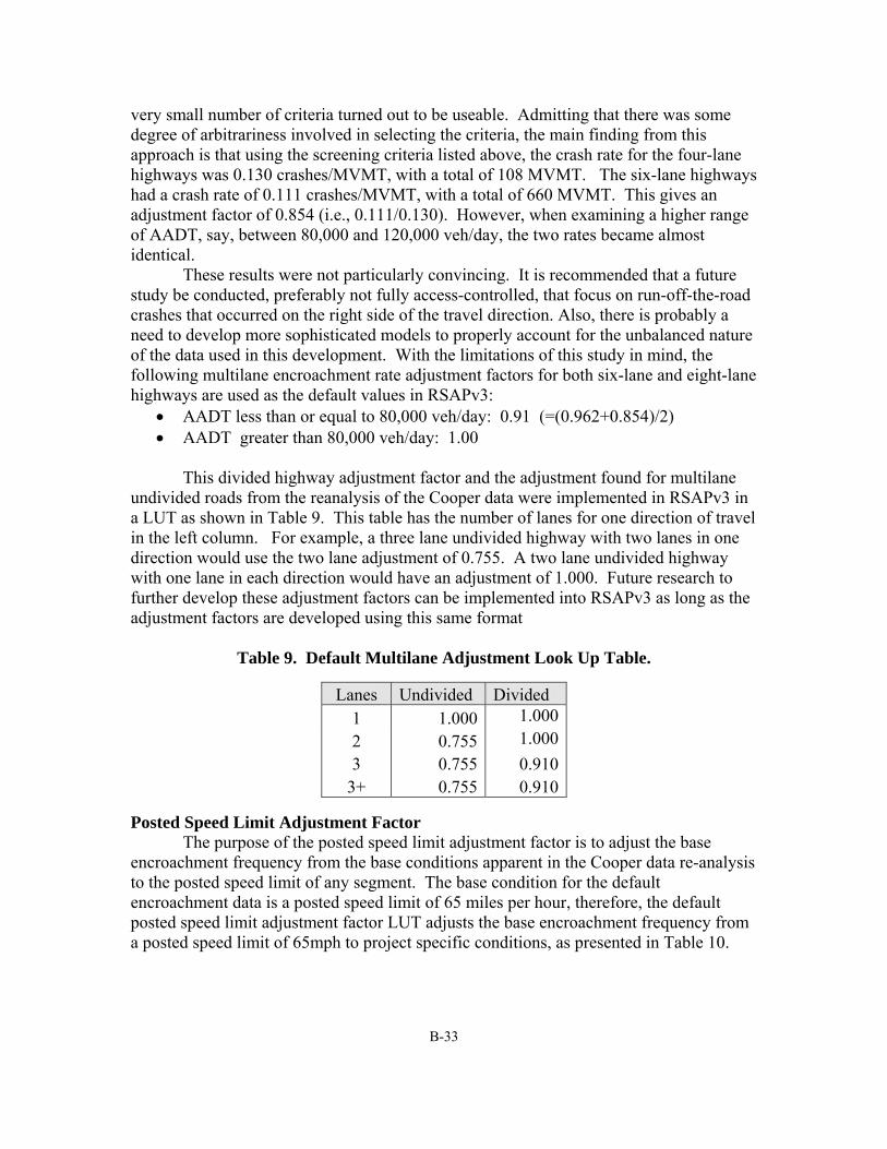
B-33

very small number of criteria turned out to be useable. Admitting that there was some degree of arbitrariness involved in selecting the criteria, the main finding from this approach is that using the screening criteria listed above, the crash rate for the four-lane highways was 0.130 crashes/MVMT, with a total of 108 MVMT. The six-lane highways had a crash rate of 0.111 crashes/MVMT, with a total of 660 MVMT. This gives an adjustment factor of 0.854 (i.e., 0.111/0.130). However, when examining a higher range of AADT, say, between 80,000 and 120,000 veh/day, the two rates became almost identical.

These results were not particularly convincing. It is recommended that a future study be conducted, preferably not fully access-controlled, that focus on run-off-the-road crashes that occurred on the right side of the travel direction. Also, there is probably a need to develop more sophisticated models to properly account for the unbalanced nature of the data used in this development. With the limitations of this study in mind, the following multilane encroachment rate adjustment factors for both six-lane and eight-lane highways are used as the default values in RSAPv3:

AADT less than or equal to 80,000 veh/day: 0.91 (=(0.962+0.854)/2) AADT greater than 80,000 veh/day: 1.00

This divided highway adjustment factor and the adjustment found for multilane

undivided roads from the reanalysis of the Cooper data were implemented in RSAPv3 in a LUT as shown in Table 9. This table has the number of lanes for one direction of travel in the left column. For example, a three lane undivided highway with two lanes in one direction would use the two lane adjustment of 0.755. A two lane undivided highway with one lane in each direction would have an adjustment of 1.000. Future research to further develop these adjustment factors can be implemented into RSAPv3 as long as the adjustment factors are developed using this same format

Table 9. Default Multilane Adjustment Look Up Table.

Lanes Undivided Divided 1 1.000 1.000

2 0.755 1.000

3 0.755 0.9103+ 0.755 0.910

Posted Speed Limit Adjustment Factor The purpose of the posted speed limit adjustment factor is to adjust the base

encroachment frequency from the base conditions apparent in the Cooper data re-analysis to the posted speed limit of any segment. The base condition for the default encroachment data is a posted speed limit of 65 miles per hour, therefore, the default posted speed limit adjustment factor LUT adjusts the base encroachment frequency from a posted speed limit of 65mph to project specific conditions, as presented in Table 10.

B-34

Table 10. Posted Speed Limit Adjustment Look Up Table.

Posted Speed Limit (mi/hr) Undivided Divided

<60 1.423 1.179

60 1.423 1.179

65 1.00 1.00

>65 1.00 1.00

Access Density Adjustment Factor One of the most interesting results of the reanalysis of the Cooper data was the

importance of access density in predicting encroachments. The purpose of the access density adjustment factor is to adjust for the number of major road and highway access points per mile in any segment. This adjustment factor is intended to represent the effect on encroachments frequency of increasing the number of major access points; the baseline access density is zero access points/mi. For both the two-lane undivided and four-lane divided highways, an increase in access density results in an increase in encroachment frequency as shown in Table 11. The adjustments can be quite large; for example, a two-lane undivided highway with more than six major access points/mi has more than 10 times the encroachment frequency of an otherwise similar roadways with no access points/mi as shown in Table 11. The access density affect decreases and levels off for both types of highways: for two-lane undivided highways an adjustment of 10.99 is used for all access densities greater than six and an adjustment of 8.56 is used on four-lane divided highways for access densities greater than three points/mi.

The Highway Safety Manual (HSM) also contains research on access density in a crash modification factor in HSM Table 13-58 of the HSM.[AASHTO10] This adjustment factor is applicable to urban and suburban arterials. The adjustment is the same for undivided and divided highways. Interestingly, this adjustment factor starts were the Table 11 adjustment factor leaves off (i.e., seven access points) and the adjustment magnitudes match quite well.

Table 11. Default Access Density Adjustment Look Up Table.

Points/mile Undivided Divided0 1.00 1.00 1 1.49 2.05 2 2.22 4.18 3 3.32 8.56 4 4.94 8.56 5 7.73 8.56 6 10.99 8.56 7 10.99 8.56

B-35

Terrain Adjustment Factor The adjustment for general terrain is used to adjust the base encroachment

frequency for segment characteristics. The sample size was too small to estimate terrain effects for divided highway, however, terrain is assumed to have half the influence of the undivided highways. The results are shown in Table 12.

Table 12. Default Terrain Look Up Table.

Terrain Undivided Divided One-Way Flat 1.000 1.000 1.000 Rolling 2.579 1.661 1.661 Mountainous 2.269 1.506 1.506

Adjustment factors are straightforward modifications not influenced by other

highway characteristics (i.e., they are assumed to be independent), therefore, this number is multiplied directly by the encroachment frequency to modify the encroachment frequency from flat terrain.

Vertical Grade Adjustment Factor Some adjustment factors in RSAPv3, like the grade adjustment are direction

dependent. For example, if the primary direction is on a negative grade the opposing direction must be on a positive grade so the adjustments for grade would be different on each side of the highway. RSAP like BCAP and Roadside used the Wright and Robertson study values show in Table 13 so if the primary direction is a downgrade at 4 percent the adjustment is 1.5 in the primary direction but 1.0 in the opposing up-grade direction. [Wright76] Unfortunately, the Wright and Robertson study uses fairly old data and had relatively few cases so the statistical reliability has always been in question.

Table 13. Wright and Robertson Grade Look Up Table.

Grade (%)

Adjustment

<-6 2.00 -6 2.00 -2 1.00 >-2 1.00

B-36

Table 14. Miaou Grade Look Up Table.

Grade (%) Adjustment

±8 8.32±7 7.28±6 6.24±5 5.20±4 4.16±3 3.12±2 2.08±1 1.04

0 1.00Miaou also developed a grade adjustment factor for rural two lane roads in 1995

based on a much larger data sample but, unfortunately, this adjustment factor does not differentiate between the directions of travel.[Miaou95] Miaou’s adjustments tends to be somewhat larger than Wright and Robertson. In the short term the Wright-Robertson data is used as the default in RSAPv3 but it is hoped that some of the data used by Miaou or the HSM can be re-examined in order to differentiate directions and improve this directional grade adjustment factor.

Horizontal Curve Adjustment Factor The horizontal curvature adjustment factor is another directionally dependent

adjustment in RSAPv3. Presumably, vehicles are more likely to encroach on the outsides of horizontal curves than on the inside but, unfortunately, there is relatively little data where the direction of travel was known in the data analysis.

Figure 3 shows the Wright and Robertson horizontal curve adjustment factor that has traditionally been used in RSAP as well as in BCAP and Roadside. Negative radii of curvature represent curves to the left (i.e., outside of curve) and positive radii represent curves to the right (i.e., inside of curve). The Wright-Robertson horizontal curve adjustment factor corresponds to what one would expect – outside of curves experience more encroachment than the insides of curves. The adjustment reaches a maximum for both outside and inside curves at a radius of about 1,000 ft (i.e., 6 degrees of curvature) but it is suspected that this was an ad hoc decision rather than a result of there being data at those radii. As with the grade adjustment factor, the Wright-Robertson study suffers from being a small relatively old dataset so, again, this adjustment has often been questioned. A study to use the HSIS or some other suitable database to determine better horizontal and vertical curve adjustments should be conducted to update these values.

B-37

B-38

Figure 3. Comparison of Horizontal Curve Adjustment Factors.

Figure 4. Horizontal Curve Adjustment Factors with HSM Symmetry Assumed.

The HSM also has a horizontal curve crash modification factor but, again,

unfortunately it is not direction dependent. The HSM CMF, however, is much more statistically sound so it is useful to examine this CMF and see if with some modifications it better accommodates roadside design evaluations. The HSM CMFs were created to evaluate total roadway crashes per segment whereas RSAPv3 evaluates only run-off-road crashes. When modeling total crashes on a segment, the direction of curvature does not influence the outcome because the road curves to the right traveling and one direction and the left traveling in the other. When modeling ROR crashes, however, using the encroachment probability model used by RSAPv3 directionality is important. The HSM horizontal curvature CMF is given as:

1.55 ∗ 80.2 0.012 ∗

1.55 ∗

Where: Lc = Length of horizontal curve including length of spriral transitions, if present (mi) R = Radius of curvature (ft)

B-39

S = 1 if spiral transition curve is present; 0 if spiral transition curve is not present.

The HSM notes the effects of the spiral transitions are small for any given radius so the presence of spiral transitions can be neglected to simplify the equation. Removing spiral transitions from the CMF (i.e., S=0) results in the following equation:

1.55 ∗ 80.2

1.55 ∗

The resulting equation was graphed over a series of curve radii and lengths to determine the effect of and the limits of these variables. The results are presented in Figure 5. The length of the curve appears to have a significant impact on the adjustment factor at short curve lengths and a decreasing impact as the length of curve increases. The length of curve has a dramatic effect at very short lengths (e.g, less than 100 feet).

Figure 5. HSM Horizontal Curve Adjustment Factor.

The HSM CMF can be algebraically rearranged as follows:

1.55 ∗ 1 80.2

1.55 ∗ 11

80.21.55

Using an adjustment factor of this form would mean that instead of the user

providing the radius of the curve as was done in earlier versions of RSAP, the quantity of the radius times the length of curve would be provided and this somewhat unconventional

B-40

curve characteristic would be used to calculate the horizontal curve adjustment factor. This adjustment yields the relationship shown in Figure 6 between the radius times curve length and the adjustment factor

Properly adjusting for horizontal curvature is an area that needs additional work. The Wright-Robertson data which accounts for directionality is small and statistically weak whereas the HSM data is statistically strong but does not account for directionality. It would be possible to re-analyze the data which the HSM CMF is based on to include directionality.

Figure 6. HSM Horizontal Curve Adjustment Factor.

Lane Width Adjustment Factor The purpose of the lane width adjustment factor is to adjust the baseline

encroachment frequency assumption of 12 foot lanes to the appropriate average lane width for each road segment. RSAP has traditionally not adjusted for lane width effects, however, the recent publication of the HSM included a CMF for the adjustment of lane widths which is applicable to run off road crashes. The HSM has many modifiers for adjusting crash predictions for lane width over a range of AADTs and highway types (i.e., divided or undivided) but the CMFs level out at a relatively low volume of 2000 veh/day so RSAPv3 conservatively uses the CMF for 2000+ vehicles for all traffic volumes. For example, given a two lane undivided highway with one segment where one lane equals 12-ft and the other lane equals 10-ft. The lane widths would be averaged to 11-ft and an adjustment of 1.05 would be applied to the encroachment frequency.

1.00

1.50

2.00

2.50

3.00

3.50

4.00

- 1.00 2.00 3.00 4.00 5.00 6.00 7.00 8.00 9.00 10.00

Ad

just

men

t

Radius x Curve Length (millions ft2)

B-41

Table 15. Default Lane Width Adjustment Look Up Table.

Lane Width

(ft) Undivided Divided0 1.50 1.25 9 1.50 1.25 10 1.30 1.15 11 1.05 1.03 12 1.00 1.00 40 1.00 1.00

Figure 7. HSM Lane Width Adjustment Factor. [AASHTO10]

9ft-2ln, 1.5

10ft-2ln, 1.3

11ft-2ln, 1.05

9ft-4ln, 1.38

10ft-4ln, 1.23

11ft-4ln, 1.04

9ft-4ln, 1.25

10ft-4ln, 1.15

11ft-4ln, 1.031

1.1

1.2

1.3

1.4

1.5

0 400 2000 2400

CM

F

AADT (vpd)

Divided Highway CMFs Undivided Highway CMFs

B-42

The HSM CMFs for AADT values ranging from zero to 400 are relatively small across all combinations of lane widths and highway types. A pronounced difference occurs at 2,000 vpd. Modeling this data to match the RSAPv3 LUT format with the interpolated value in the first column, the undivided highway adjustment in the second column and the divided highway adjustment in this third column, the resulting data table was developed and shown in Table 15.

Adding New Encroachment Data and Adjustment Factors The base encroachment frequencies and the adjustment factors have been

developed for divided and undivided highway types and the behavior of one-way roads have been extrapolated from the divided highway data. The base encroachment frequency table and the adjustment factor LUTs are all located in RSAPv3 on the “Encr Freq and Adj” worksheet. All encroachment frequency and encroachment adjustment look-up tables have four columns. The first column always contains the independent variable. For example, the first column for the Encroachment Frequency LUT is AADT. The first column for in the Grade Adjustment LUT is GRADE.

The second through fourth columns contain the corresponding adjustment factor for two-lane undivided, four-lane divided and one-way roadways respectively (i.e., two-lane undivided is in column 2, four-lane divided is in column 3 and one-way is in column 4). All the tables function as interpolation tables where RSAP enters the table with the desired independent variable and performs a linear interpolation to find the appropriate value. When creating new LUTs it is important that the first value and the last value are at the very extremes of the expected data so that it is impossible for a value to be entered that is outside the range of the table. If this occurs the table will not interpolate correctly.

New research on encroachment frequency and adjustment factors can easily be incorporated into RSAPv3 provided the results of the research are tabulated as shown above and discussed here. Once a new adjustment LUT or base encroachment LUT is created it can be added to RSAPv3 as follows: First, open an RSAP Excel workbook select the “Encr Freq and Adj” tab on the bottom of the RSAPv3 screen. Worksheets in RSAPv3 are protected to prevent unintended changes to the program or data so the workbook needs to be unprotected in ordered to add data. Select any cell in the “Encr Freq and Adj” worksheet and press CTRL+SHIFT+E. This key stroke will unprotect all the worksheets and allow the worksheet to be edited using the usual Excel functionality. Add the new information to one of the existing LUTs in the worksheet. Excel formulae can be used in the LUTs or simple numeric values can be used. The values must proceed in increasing order for the independent variable (i.e., first column). Make sure there are no blank rows in the LUT. When all the desired edits have been made, press CTRL+SHIFT+E again to re-protect the worksheet and re-start RSAPv3. CTRL+SHIFT+E is a toggle which turns the program editing state on if it is off and off if it is on. RSAPv3 will now use the updated LUTs in the “Encr Freq and Adj” worksheet.

B-43

VEHICLE TYPES

Vehicle Classifications In the 1980’s FHWA established a 13-vehicle classification system and started

asking the states to report data using these classifications when possible. [FHWA01] For many years, data has been collected and reported using the following thirteen classes:

1. “Motorcycles (Optional) All two or three-wheeled motorized vehicles. Typical vehicles in this category have saddle type seats and are steered by handlebars rather than steering wheels. This category includes motorcycles, motor scooters, mopeds, motor-powered bicycles, and three-wheel motorcycles. This vehicle type may be reported at the option of the State.

2. Passenger Cars All sedans, coupes, and station wagons manufactured primarily for the purpose of carrying passengers and including those passenger cars pulling recreational or other light trailers.

3. Other Two-Axle, Four-Tire Single Unit Vehicles All two-axle, four-tire, vehicles, other than passenger cars. Included in this classification are pickups, panels, vans, and other vehicles such as campers, motor homes, ambulances, hearses, carryalls, and minibuses. Other two-axle, four-tire single-unit vehicles pulling recreational or other light trailers are included in this classification.

4. Buses All vehicles manufactured as traditional passenger-carrying buses with two axles and six tires or three or more axles. This category includes only traditional buses (including school buses) functioning as passenger-carrying vehicles. Modified buses should be considered to be a truck and should be appropriately classified.

5. Two-Axle, Six-Tire, Single-Unit Trucks All vehicles on a single frame including trucks, camping and recreational vehicles, motor homes, etc., with two axles and dual rear wheels.

6. Three-Axle Single-Unit Trucks All vehicles on a single frame including trucks, camping and recreational vehicles, motor homes, etc., with three axles.

7. Four or More Axle Single-Unit Trucks All trucks on a single frame with four or more axles.

8. Four or Fewer Axle Single-Trailer Trucks All vehicles with four or fewer axles consisting of two units, one of which is a tractor or straight truck power unit.

9. Five-Axle Single-Trailer Trucks All five-axle vehicles consisting of two units, one of which is a tractor or straight truck power unit.

10. Six or More Axle Single-Trailer Trucks All vehicles with six or more axles consisting of two units, one of which is a tractor or straight truck power unit.

11. Five or fewer Axle Multi-Trailer Trucks

B-44

All vehicles with five or fewer axles consisting of three or more units, one of which is a tractor or straight truck power unit.

12. Six-Axle Multi-Trailer Trucks All six-axle vehicles consisting of three or more units, one of which is a tractor or straight truck power unit.

13. Seven or More Axle Multi-Trailer Trucks All vehicles with seven or more axles consisting of three or more units, one of which is a tractor or straight truck power unit.” [FHWA01]

In prior versions of RSAP 13 vehicle classes, not exactly corresponding to the

FHWA 13 classes, were included in the calculations but this seems unnecessary for several reasons. First, some of the vehicle classes represent a very small proportion of vehicle miles travelled and that only on high-speed high-volume roadways. For example, Table 16 shows the vehicle traffic volumes from Maryland in 2008. Classes 4 through 13 represent 8.39% of the total vehicle miles travelled and 5.87% are represented by just two truck classes (i.e., class 5: two-axle six-tire single unit trucks and class 9: 5-axle single-trailer trucks). Multi-trailer trucks (i.e., classes 12 and 13) represent less than 1% of the vehicle miles travelled. Many of these vehicle types simply do not account for much traffic on the roadways, especially when undivided roadways are considered. Second, there are no trajectory data for any vehicle types other than passenger vehicles so adding many vehicle types simply adds computational time without much additional benefit. For these reasons RSAPv3 initially is set up to use three vehicle types: motorcycles (i.e., FHWA Class 1), passenger vehicles (i.e., FHWA Class 2 and 3) and trucks (i.e., FHWA Classes 4 through 13). As will be discussed in the next section, additional vehicle types can be easily added to RSAPv3 but the computation time is directly proportional to the number of vehicle types (i.e., an analysis with six vehicle types will take twice as long as an analysis with three vehicle types). Additional vehicle types really only need be added if collisions involving a variety of trucks is of particular concern. For example, if developing warranting criteria for multiple test level barriers where the barrier heights and capacities are different the analyst would probably like to add vehicles matching the vehicles appropriate for that test level.

B-45

Table 16. Maryland 2008 Vehicle Distribution by Vehicle Class

Vehicle Class Distribution

1 0.31%2 78.21%3 13.00%4 0.70%5 2.65%6 0.85%7 0.19%8 0.62%9 3.22%

10 0.10%11 0.09%12 0.03%13 0.03%

Table 17 shows the recommended vehicle properties for use in RSAPv3 based on

the thirteen different FHWA vehicle classes. The values were derived from a variety of sources, many of which were discussed in the previous section. RSAPv3 uses these vehicle properties for predicting structural penetration of features and for predicting rollover during interaction with features (e.g., roll-over-the-barrier and rollover during redirection from barrier). For vehicle classes 1 through 3, only the vehicle weight property is required for the analysis since rollover is determined solely from crash statistics for those classes of vehicles. The other five vehicle properties listed for vehicle classes 1 through 3 are for informational purposes only.

B-46

Table 17: Recommended vehicle properties for use in RSAPv3 based on the 13 FHWA vehicle classes

Vehicle Type FHWA Class

RSAP Type

Weight Length Width C.G. Long.

C.G. Vert.

(lbf) (ft) (ft) (ft) (ft) motorcycles 1 M 490 7.2 3 3.6 2.7cars 2 C 3200 16 6 4.8 1.9pickups and vans 3 V 3732 18 6 7 2.3buses 4 B 40000 40 8 22 582-axle SUT 5 2SUT 22000 35 8 12.5 4.23-axle SUT 6 3SUT 4+axle SUT 7 4SUT 4-axle Single Trailer 8 4TT 5-axle single trailer 9 5TT 80000 62 8.5 24 5.46+axle single trailer 10 6TT 5-axle multi-trailer 11 5MT 6-axle multi-trailer 12 6MT 7+axle multi-trailer 13 7MT

cars and vans 2, 3 C 3413 16.8 6 5.7 2.1trucks 4, 13 T 40560 43.6 8.2 16.2 4.6

Passenger Cars The vehicle weight property for passenger cars in Table 17 were derived from the

three “passenger” vehicle types in NCHRP Report 492 using a weighted average based on the vehicle fleet distribution.[Mak03] For example, the passenger car fleet in Report 492 was shown to be comprised of 15 percent of 820-kg vehicles (i.e., 8.1/(8.1 + 33.8 + 12.1), 62.6 percent of 1410-kg vehicles, and 22.4 percent of 2000-kg vehicles. The resulting weighted average is thus 1454 kg or 3,200 lb. The remaining properties for the passenger car vehicle class were obtained from the NCAC Ford Taurus finite element model.[NACA12]

Pickup Trucks, Vans and Sport Utility Vehicles The vehicle weight property for passenger trucks and vans in Table 17 were also

derived using a weighted average of vehicle weights in NCHRP Report 492 based on the vehicle fleet distribution, resulting in a representative value of 3,732 lb. The remaining

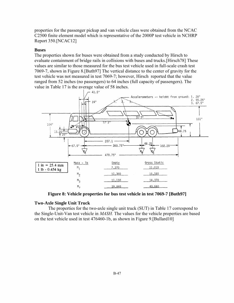
B-47

properties for the passenger pickup and van vehicle class were obtained from the NCAC C2500 finite element model which is representative of the 2000P test vehicle in NCHRP Report 350.[NCAC12]

Buses The properties shown for buses were obtained from a study conducted by Hirsch to evaluate containment of bridge rails in collisions with buses and trucks.[Hirsch78] These values are similar to those measured for the bus test vehicle used in full-scale crash test 7069-7, shown in Figure 8.[Buth97] The vertical distance to the center of gravity for the test vehicle was not measured in test 7069-7; however, Hirsch reported that the value ranged from 52 inches (no passengers) to 64 inches (full capacity of passengers). The value in Table 17 is the average value of 58 inches.

Figure 8: Vehicle properties for bus test vehicle in test 7069-7 [Buth97]

Two-Axle Single Unit Truck The properties for the two-axle single unit truck (SUT) in Table 17 correspond to

the Single-Unit-Van test vehicle in MASH. The values for the vehicle properties are based on the test vehicle used in test 476460-1b, as shown in Figure 9.[Bullard10]

B-48

Figure 9: Two-axle SUT test Vehicle properties for test 476460-1b [Bullard10]

Five-Axle Tractor-Semitrailer Vehicle The properties for the five-axle single trailer vehicle (i.e., FHWA Class 9) in Table 17

correspond to the tractor-van-trailer test vehicle in MASH and Report 350. The values for the vehicle properties were adopted from the test vehicle used in test TL5CMB-2, as shown in Figure 11.[Rosenbaugh07]

When a tractor-semitrailer vehicle impacts a barrier, the following general series of events occur, which are illustrated in Figure 10:

B-49

(1) Tractor impacts and, if structural penetration does not occur, then starts redirecting along the barrier. In this phase of the impact, the vehicle is not likely to rollover the barrier since the center of gravity of a tractor is only approximately 2.5 ft above ground.

(2) The rear tandem axle of the tractor and the front of the trailer impact the barrier simultaneously, and a second peak force results. Again, if structural penetration does not occur, the tractor continues its path parallel to the barrier and the trailer begins its redirection.

(3) As the trailer is redirecting, the friction generated between the rear tandem tires on the trailer on the ground cause the trailer to roll toward the barrier.

(4) Then when the rear tandems on the trailer impact against the barrier, a third peak force is generated. The location of the impact force is somewhat below the center of gravity of the trailer (e.g., c.g. is approximately 6 ft), thus the trailer increases its roll angle toward the barrier.

(5) As the trailer is rolling onto the top of the barrier, the tractor acts as a “dead weight” that tends to counter the roll motion of the trailer, preventing it from rolling over the barrier.

Figure 10: Illustration of collision sequence in tractor-semitrailer impacts with longitudinal barriers (Test TL5CMB-2)[Rosenbaugh07]

If the trailer were not connected to the tractor, however, the mass of the trailer and its high center of gravity would likely result in the trailer rolling over longitudinal safety barriers in even the most benign impact conditions. The equations in RSAPv3 for predicting if the vehicle will roll over the barrier during collision were derived based on a single-unit-vehicle model; however, they provide reasonable predictions for single trailer articulated vehicles with the following simple modifications to the vehicle properties. The longitudinal distance to the c.g. should be measured from the front of the trailer to the center of gravity of the trailer, rather than measuring the distance from the front of the tractor to the overall center of gravity of the tractor-trailer vehicle. The property value listed in Table 17 is the distance measured to the center point of the trailer. The vertical c.g. height, however, should correspond to the average c.g. of the overall tractor-trailer vehicle. This value is not generally measured for the test vehicles used in compliance tests of roadside safety barriers and its value is difficult to find in the literature. The vertical c.g. height for the 5-axle single trailer vehicle in Table 17 was obtained from the finite element model of the test TL5CMB-2 tractor-semitrailer test vehicle developed by

B-50

NCAC and Battelle for the National Transportation Research Center, Inc. (NTRCI). [Plaxico09]

B-51

Figure 11: Vehicle properties for tractor-van-trailer test vehicle used in Test

TL5CMB-2

Date: Test Number:

Tractor:VIN No,: Make: Model:

Year: Odometer:

Trailer:VIN No,: Make: Model:

Year:

*All Measurements Refer to Impacting Side

Vehicle Geomerty -mm (in)

A 2,604 (102.5) G 5,906 (232.5) N 0 (0.0) T 1,016 (40.0)

B 1,314 (51.7) H 1,831 (72.1) O 584 (23.0) U 597 (23.5)

C 3,270 (128.7) J 1,746 (68.7) P 2,007 (79.0) V 781 (30.7)

D 1,334 (52.5) K 1,575 (62.0) Q 1,842 (72.5) W 4,064 (160.0)

E 10,185 (401.0) L 1,156 (45.5) R 1,981 (78.0) X NA

F 1,257 (49.5) M 902 (35.5) S 533 (21.0)

Mass -PropertiesM1 3,973 (8,759) 4,441 (9,791) 4,441 (9,791)

M2 + M3 5,144 (11,341) 17,017 (37,516) 17,017 (37,516)

M4 + M5 3,955 (8,719) 14,696 (32,399) 14,696 (32,399)

MTotal 13,073 (28,821) 36,154 (79,706) 36,154 (79,706)

I11 (0) (0) (0)

I22 (0) (0) (0)

I33 (0) (0) (0)

WG65T1991 137548

1p10748254jka29485 Pines 48'

kg - m2 (lb-ft2)

7/12/2007 MwRSF Test No. TL5CMB-2

4V1JLBJEGMR810558 White/GMC

kg - m2 (lb-ft2)

48' Van1988

Curb Test Inertial Gross Statickg (lb)kg (lb)kg (lb)kg (lb)

kg - m2 (lb-ft2)

B-52

Combined Vehicle Categories The default vehicle properties listed in the “Traffic Information” worksheet include three vehicle types: (1) motorcycles, (2) passenger vehicles and (3) trucks. The properties for the motor cycle vehicle group were adopted directly from Table 17. The properties for the passenger vehicles are representative of all passenger cars, pickups and vans (i.e., FHWA classes 2 and 3) and were derived from the values in Table 17 using a weighted average distribution of vehicle types from NCHRP Report 492. Passenger cars are presumed to represent 54 percent of the total vehicle fleet, while pickup truck, vans and other sport utility vehicles represent 36 percent of the fleet. Thus, for example, the representative value for passenger vehicle weight was computed by:

.

3200 ∗ 54% 3732 ∗ 36%54 36 %

3413

The remaining properties for passenger vehicles were derived in the same manner.

The properties for trucks were derived in a similar manner using the data in Table 17 for two-axle single unit trucks (i.e., FHWA Class 5) and five-axle single trailer trucks (i.e., FHWA Class 9). The distribution between SUT’s and five-axle tractor-trailers was taken from Harwood study and used to computed the weighted-average vehicle properties, where SUTs represent 68 percent of the truck fleet and tractor-trailers represent 32 percent.[Harwood03] The default vehicle properties table used on the “Traffic Information” worksheet is shown in Table 18.

Table 18. Default RSAPv3 Vehicle Properties Table

RSAP VEHICLES

FHWA CLASS

WEIGHT LENGTH WIDTH C.G. Long.

C.G. Hgt

Crash Cost Adj. lbs ft ft ft ft

Motorcycles 1 600 7.00 1.50 3.00 2.60 0.56

Passenger Vehicles 2-3 3,400 15.00 5.40 6.00 2.00 1.00

Trucks 4-13 50,000 28.00 8.00 13.00 4.20 3.52

Adding New Vehicle Types RSAPv3 includes three default vehicle types: passenger vehicles, motorcycles and trucks as shown in Table 18. Additional vehicle types can be easily added although care should be used in added additional vehicle types since computer run time increases proportionally to the number of vehicles (i.e., a run with six vehicle types will require twice as long as a run with three vehicle types regardless of the traffic mix) Prior to adding a new type of vehicle the following information must be collected: To add a new hazard to RSAPv3, the following information is required:

B-53

A unique name for the vehicle type that is not already used in RSAP v3, The FHWA vehicle classification (optional), The percent of traffic associated with the new vehicle type, A one-letter unique identifier that is not already used by RSAPv3, The typical weight, length and width, The height and distance from the front bumper of the center of gravity, A crash cost adjustment factor for the new vehicle type, The name of the trajectory grid worksheet and The name of the redirection grid worksheet.

The crash cost adjustment factor is a value that is applied to the crash costs to account

for the difference in crash costs for different vehicles. For example, large truck crash costs tend to be 3.52 times greater than typical passenger car costs so an adjustment of 3.52 is used. If a study is not available to determine the appropriate adjustment use 1.0 for passenger vehicle like classes and 3.52 for large trucks and buses.

RSAPv3 uses two trajectory grids for plotting the trajectory of vehicles during an encroachment. Currently there is only data for passenger car trajectories but if new trajectory information is obtained it can be added to the appropriate worksheet. Unless new trajectory information is available enter “TrajectoryGrid2” the trajectory grid name and “RedirectionCars” for the redirection trajectory grid.

Once this information is collected it can be entered into the RSAPv3 database as follows. First, open an RSAP Excel workbook and either select the “Traffic Information” tab on the RSAPv3 controls or go to the “Traffic Information” worksheet. Worksheets in RSAPv3 are protected to prevent unintended changes to the program or data so the workbook needs to be unprotected in ordered to add data. Select any cell in the Traffic Information worksheet and press CTRL+SHIFT+E. This key stroke will unprotect all the worksheets and allow the worksheet to be edited using the usual Excel functionality

Add the information collected above to the Vehicle Mix table using the next open available row. Make sure there are no blanks in the table. A list of the classification numbers for each RSAP vehicle type should be entered in the “FHWA CLASS” column. The entry should be a comma delimited list when more than one FHWA classification is included for an RSAP vehicle type. For example, “Passenger Vehicles” includes both passenger cars and pickup trucks, SUVs and minivans so “2,3” is entered under “FHWA Class.” When all the desired edits have been made, press CTRL+SHIFT+E again to re-protect the worksheet re-start RSAPv3. CTRL+SHIFT+E is a toggle which turns the program editing state on if it is off and off if it is on. It is very important to restart RSAP by re-toggling CTRL+SHIFT+E since this re-builds all appropriate menus and internal databases.

CRASH PREDICTION MODULE The probability of a collision given that a vehicle has encroached onto the

roadside or median is determined in RSAPv3 by directly projecting reconstructed vehicle trajectories onto the roadside or median and determining if the trajectory intersects the position of any roadside hazard. RSAPv3 includes three general types of hazards:

B-54

1. Point hazards, 2. Line hazards and 3. Area hazards. Point hazards are generally items like signs, trees utility poles and other roadside

features that can be reasonably approximated as a point in space. Line hazards are those features that can be approximated by a line including longitudinal barriers (i.e., guardrails, bridge railings, median barriers, etc.) and some special features like the edge-of-clearzone, edge-of-median, water hazards, and tree-lines. Area hazards are generally related to terrain features like slopes and ditches and involve vehicle rollover. The “hazard type” for each hazard is defined in column B on the RSAPv3 “Severity” worksheet. When conducting an RSAPv3 analysis for a segment of roadway, the point and line hazards are defined explicitly by type and location on the RSAP “Alternatives” worksheet. Area hazards (i.e., rollover), on the other hand, are defined automatically in RSAPv3 and are determined based on terrain geometry (e.g., side-slope) and other roadway conditions. In essence, there is always a risk of rollover on any terrain so RSAPv3 always examines the terrain to determine the likelihood of rollover during the trajectory.

Figure 12 provides a simplified representation of the steps which the crash prediction module takes to determine if a collision occurs; if a terrain rollover occurs; or if nothing happens and the encroachment results in a non-crash event.

As shown in Figure 12, trajectories are first selected for a uniform segment of road. The method used to select trajectories is explained in the following section. After the appropriate trajectories have been selected, the trajectories are mapped onto the roadside and/or median at the start of the uniform segment as defined by the user. Each trajectory is examined for a possible collision with a modeled hazard at pre-selected increments along the trajectory path (e.g., the default increment is four feet).

When examining a trajectory, there are many possible outcomes. For example, a trajectory may interact with a roadside hazard, then either stop in contact, penetrate, or be redirected. The probability of each of these events is calculated and the outcome of each sub-event is evaluated. Continuing with the same example, if the vehicle penetrates the barrier, the trajectory is followed further to determine if it interacts with any other modeled hazards or results in a rollover. If the trajectory is redirected, the redirected paths are evaluated. After all of the possibilities have been exhausted, the selected trajectories are incremented forward a predetermined amount along the segment to continue the analysis. The following sections discuss the methodology that RSAPv3 uses in trajectory selection, determining probability of rollovers due to “soil-tripping” and determining probability of hazard penetration.

B-55

Figure 12. RSAPv3 Crash Prediction Module Flow Chart.

TRAJECTORY LOOK UP TABLE The driver’s response (i.e., steer maneuver, braking or acceleration) after the

vehicle encroaches onto the roadside may be affected by several factors such as roadside terrain, environmental conditions, driver alertness, etc. all of which contribute to the resulting trajectory of the vehicle. Another important factor that will influence vehicle trajectory is the driver’s response when trying to avoid roadside objects in an impending

1. Select trajectories for a

uniform segment.

2. Map selected trajectories onto

roadside.

3. Examine trajectories for intersections with hazards.

4. Collision is detected.

4a. Probability of rollover

before collision?

4b. Probability of penetrating

hazard?

4c. Probability of redirection?

Repeat analysis.

5. No collision detected.

Probability of terrain rollover?

6. Increment forward.

B-56

crash. Trajectory data that comes from non-crash related studies (e.g., Cooper data, numerical simulation, etc.) will not account for the influence of crash avoidance and may bias the trajectory data toward more “unrealistically” controlled departure conditions. Crash data studies, on the other hand, collect data from actual crash events in which driver response related to crash avoidance is inherently included. It is therefore presumed that trajectory data from crash cases are more applicable to RSAP since RSAP is primarily concerned with determining probability of impact and corresponding impact severity/cost.

Currently, the RSAPv3 trajectory look up table is populated with the trajectories collected under NCHRP Project 17-22, which generated a run-off road (ROR) crash reconstruction database. The NCHRP 17-22 team assembled a database of 890 crash cases which is composed of data collected from the FHWA rollover study, NCHRP Project 17-11 and new cases added under NCHRP Project 17-22.[Bligh08; Mak10]

A significant advantage of using crash reconstruction databases is that they are based on real drivers’ responses in actual crash events. Unfortunately, however, trajectories from crash data terminate abruptly at the point of impact and it is not possible to discern exactly what the trajectory would have been beyond that point had impact not occurred. Considering all 890 cases in the NCHRP 17-22 Crash Reconstruction Database, the velocities at impact ranged from 4.2 mph to 93.6 mph with mean value of 39.13 mph and standard deviation of 16.45 mph [Albuquerque10], which suggests that some of the trajectories would have continued for significant distances. It could be argued that an estimate of the continuation of the trajectory paths beyond the impact point could be obtained from the curve fit function developed from the available data; but there is no way to confirm that the extended trajectories would be realistic or even appropriate.

The primary advantage of not extrapolating the trajectory data is that no assumptions are made about probable trajectory paths beyond the information available in the crash database. As a consequence, however, the farther downstream of the departure point one considers, less and less trajectory information will be available for developing statistically significant probabilities of the trajectory paths. This is better understood from viewing the cumulative distribution charts, shown in Figure 13, which show the cumulative distribution of all trajectories in the NCHRP 17-22 Crash Reconstruction Database. These charts show the percent of crash cases with longitudinal and lateral trajectories distances exceeding given values; they also show the number of crash cases with trajectories distances exceeding given values. In other words, Figure 13 indicates that at locations very near the departure point there is adequate data for developing statistical information; whereas at 177 ft (54 m) downstream of the departure point there are less than 90 cases with trajectory information available, and at 387 ft (118 m) downstream of the departure point there are less than 15 cases with trajectory information available.

The cumulative distribution charts can also be used verify that extrapolated trajectories do not result in unrealistic conditions. For example, the chart shows that 50 percent of impacts involve hazards located less than 60.7 ft (18.5 m) downstream of the point of departure. Also, only 10 percent of impacts occur when hazards are located more than 178.8 ft (54.5 m) downstream of the point of departure, and only three percent occur when hazards are located more than 328 ft (100 m) downstream of departure. Likewise, 50 percent of impacts involve hazards located within 14.1 ft (4.3 m) lateral

B-57

offset from the roadway; only 10 percent of impacts occur when hazards are located more than 37.1 ft (11.3 m) lateral offset from the roadway; and only three percent occur when hazards are located more than 61 ft (18.6 m) lateral offset from the roadway. So, for example, in cases where the hazard is located 328 ft (100 m) downstream of departure, extrapolated trajectories should not result in a number of probable impacts significantly higher than three percent according to the crash statistics.

It is important to note that the vehicle trajectory leading up to impact is likely influenced by the driver’s response to the presence of the hazard. When a hazard is located near the departure point, a driver will have less time to respond to the approaching hazard and thus may execute more aggressive steering and braking maneuvers, compared to cases where a hazard is located farther downstream. Ideally, the trajectory information used in an RSAP analysis would come only from those trajectory cases that correspond to the exact characteristics of the segment of roadway and roadside being investigated, including the type and location of the hazard. For example, if the segment of roadway in question includes a guardrail terminal located 32.8 ft (10 m) downstream of departure, 9.8 ft (3 m) from the edge of the roadway, on a 6:1 roadside slope, then it may not be appropriate to compute probable trajectories using crash data where a terminal was located 164 ft (50 m) downstream of departure, even if all other characteristics of the roadway and roadside are the same; because, as previously discussed, the driver’s response to the hazard may have influenced the trajectory.

Unfortunately, the limited number of cases resulting from such stringent filtering of crash data would be too small to be relevant. So, even though extrapolation is not preferred, it is considered necessary at present due to the limited number of crash cases in the database. There is an on-going data collection effort under NCHRP Project 17-43 to collect additional trajectory data.[Gabler12] As this and any other additional trajectory data is collected it should be appended to the “Trajectory Grid” worksheets in RSAPv3. This makes future updates to the trajectory table straightforward and simple, and the need for extrapolation should reduce as more and more data is added.

In the current application, the reconstructed trajectory path is extrapolated beyond the collision point based on the last known trajectory information. That is, it is assumed that the vehicle continues in a straight path corresponding to the last known velocity vector, the vehicle continues to decelerate at the last known braking rate (e.g., assuming constant average deceleration), and the trajectory path terminates when velocity reaches zero.

B-58

Figure 13: Cumulative distribution chart showing percent of crash cases with

longitudinal and lateral trajectories exceeding given values

Since each trajectory case in the 17-22 database is linked directly to its corresponding roadway and roadside characteristics, it is a simple process to filter the trajectory data and select only the trajectory cases with characteristics similar to those for the roadway segment being analyzed. This eliminates the need to have multiple trajectory tables in which each corresponds to a different set of roadway and roadside conditions. The procedure for selecting relevant trajectories from the database is discussed in the following sections.

0100200300400500600700800

0%

20%

40%

60%

80%

100%

0.00 50.00 100.00 150.00

Num

ber o

f Cra

sh C

ases

CDF

(% G

reat

er)

Longitudinal Distance to Impact Point (m)

0100200300400500600700800

0%

20%

40%

60%

80%

100%

0.00 5.00 10.00 15.00 20.00 25.00 30.00

Num

ber o

f Cra

sh C

ases

CDF

(% G

reat

er)

Lateral Distance to Impact Point (m)

90th Percentile = 3.9 m (12.8 ft)10th Percentile = 54.5 m (179 ft)

90th Percentile = 1.0 m (3.3 ft)10th Percentile = 11.3 m (37 ft)

0.00

B-59

TRAJECTORY SELECTION RSAPv3 searches the trajectory database to identify relevant cases based on

similarity to segment characteristics; that is, the program selects all trajectories which have characteristics that fall within an acceptable range of characteristics defined for the segment. Each trajectory case in the 17-22 database includes the accompanying roadway and roadside characteristics.

There are many roadway and roadside characteristics listed for each crash case in the 17-22 database; any or all of these could be used to further refine the trajectory selection to more closely match the segment characteristics. However, trajectory selection criteria which are too stringent may lead to too few trajectories being used in the analysis and selection criteria that are too broad would include cases on terrain bearing little resemblance to the terrain indicated by the user for the analysis segment. In RSAPv3 the selection criteria has been limited to the four roadway and roadside characteristics believed to have the most influence on vehicle trajectory, namely:

Roadside cross-section profile, Horizontal curve radius, Highway vertical grade, and Posted speed limit. Of these four characteristics, it is believed that the roadside cross-section profile

will have the most significant effect on vehicle trajectory. For example, the trajectory path for a vehicle on a constant 4:1 fill slope is likely quite different from the trajectory path for a vehicle 4:1 v-ditch or a 4:1 cut slope. The change in slope would not only affect the path of the vehicle, but also its deceleration.

Horizontal curve radius is also considered to influence trajectory path. For example, as a vehicle encroaches onto the roadside on the outside of a curve (i.e., the road curves away) the vehicle’s path will take it farther and farther away from the roadway, resulting in much greater extent of lateral encroachment.

Highway vertical grade was not considered to have a significant influence on trajectory path; however, it may have an influence on encroachment speeds and vehicle deceleration during the encroachment event.

The posted speed limit probably has the least influence on the trajectory (i.e., path, velocity and deceleration). This research has found through examination of the 17-22 database that vehicles encroach onto the roadside at a wide range of speeds regardless of the posted speed limit; however, the average departure speed typically corresponded to approximately 90% of the posted speed when the speed limit was 50 mph or higher, and approximately 97% of the posted speed when the posted speed was 45 mph.

As previously mentioned, there are a limited number of trajectories included in RSAPv3 since the only suitable data at this time is the 17-22 reconstructed crash database. As additional trajectories are collected and added to RSAPv3, these same selection criteria can be applied to the larger dataset, however more stringent boundaries can be set using the analysis settings on the RSAP controls dialog box to control the range of similarities considered acceptable.

Adding new trajectories to RSAP is straightforward. First, start RSAP and with the cursor on the worksheet select CTRL+h. This keystroke unprotects and unhides all worksheets in the workbook. There are many hidden worksheets in RSAP that are used

B-60

to store default information. Great care should be taken while the workbook is unprotected since the macros controlling RSAP presume that particular information is located in particular places in the workbook. Once the workbook is unprotected and the hidden sheets are exposed, go to one of the trajectory worksheets. Currently there are four trajectory worksheets:

1. TrajectoryGrid1 – currently this worksheet is identical to TrajectoryGrid2 but it is provided as a place to store trajectories suitable for motorcycle encroachments. Since there are currently no trajectory databases for motorcycle encroachments, the 17-22 passenger vehicle trajectories are used.

2. TrajectoryGrid2 – this is the usual default worksheet which contains encroachment trajectory information based on the passenger car trajectory data in the NCHRP 17-22 data.

3. TrajectoryGrid3 – currently this worksheet is identical to TrajectoryGrid2 but it is provided as a place to store trajectories suitable for truck encroachments. Since there are currently no trajectory databases for truck encroachments, the 17-22 passenger vehicle trajectories are used.

4. RedirectionCars – this worksheet is for the trajectories of passenger vehicles once they are redirected from a longitudinal barrier.

5. RedirectionTrucks – this worksheet is similar to the RedirectionCars worksheet but is used for the redirection trajectories of trucks.

The TrajectoryGrid1, TrajectoryGrid2 and TrajectoryGrid3 worksheets use data directly from the 17-22 crash reconstruction database. The first column identifies the study where the trajectory was obtained. Columns B through AB provide a variety of roadway and traffic characteristics associated with the trajectories. Some of these are used in selecting the trajectories as described above. Columns AC through AR contain the lateral and vertical coordinates defining the roadside or median profile for each crash reconstruction case. Columns AS through AU provide additional information about the roadside cross-section, including max lateral extent, max vertical coordinate, and the max slope. Column AV provides the average deceleration of the vehicle from the point of encroachment to the point of impact in the 17-22 crash reconstruction database. Finally, columns AX through MK provide the lateral coordinates of the trajectory path at 1-ft longitudinal increments.

New trajectories can be added simply by appending new information to the worksheet. Any new information should be added to the bottom taking care to leave no blank rows of data. All the normal Excel functionality is available in this mode of operation so data can be cut and pasted from another worksheet or manually entered. When the data has been entered into the worksheet press CTRL+h again to return to the normal RSAP mode. Press CTRL+s to start RSAP.

Trajectory Selection Methodology RSAPv3 uses a basic methodology for selecting trajectories to include in the

analysis. This methodology involves examining and scoring each individual trajectory case based on a quantitative comparison of the four critical roadway characteristics (i.e., roadside cross-section profile, horizontal curve radius, highway vertical grade, and posted speed limit) to those in the current project section as defined by the user. The individual

B-61

scores for each of the four criteria are then combined into a single representative composite score for the trajectory case. After all trajectories have been assigned a score, RSAPv3 then selects the trajectories with the highest scores for use in the analysis.

Cross-Section Profile Score and Acceptance Criteria The roadside cross-section for each crash case in the trajectory database is

compared directly to that of roadway being analyzed and is given a score which represents its degree of similarity. The score is calculated based on the sum of the residual errors squared from a point-to-point comparison of the roadside slope coordinates, as defined below:

1∑∑

(1)

Where,

s thesimilarityscoreforcriterion1 i. e. , X SectionProfile z thei verticalcoordinatevaluefortheroadsegmentX sectionz thei verticalcoordinatevalueforX sectionofthe17 22crashcasey thei lateralcoordinatevaluefortheroadsegmentX section

As an example, Figure 14 shows the comparisons of several cross-section pairs

and the corresponding score computed using the method described above. Based on visual inspection of these cross-section pairs and the computed score, a general interpretation of the degree of similarity was established as follows:

Score of 0.93 or higher represents very good agreement; Score of 0.85 to 0.93 represents reasonable agreement; Score of 0.8 to 0.85 represents less than desirable but acceptable

agreement; Score of 0.7 to 0.8 indicates poor agreement; and Scores less than 0.7 should not be considered.

When calculating a single composite score, it is necessary to ensure that the scores for each individual characteristic have the same range of “acceptable” values. In other words, a score of 0.93, for example, should represent the same level of similarity for one characteristic as it does for another. Therefore, the scoring criteria for the remaining characteristics were developed according to these same acceptance ranges.

Obviously, the more unusual or complicated a cross-section is the more difficult it will be to find enough suitable trajectories for analysis.

B-62

Figure 14. Comparison of cross-section pairs and corresponding similarity scores.

B-63

Horizontal Curve Radius Score and Acceptance Criteria RSAPv3 recognizes tangents and circular curve segments of the horizontal

alignment of the highway. Recall the highway is divided into homogeneous segments which are comprised of the same characteristics from the start of the segment to the end of the segment. A curved segment, therefore, would have the same radius curve from start to end. A tangent segment would have no curves. Each segment is considered independent of the segment before and after it. Currently, there are only trajectory data for circular curves and tangents, data has not been gathered for spiral curves and compound curves are not possible given the segment definition. A comparable circular curve should be used to model spiral curves and a series of segments each with a different curvature should be used for compound curves.

Horizontal curves are defined by radii, in feet and direction of curvature by sign (i.e., positive curves to right and negative to left) relative to the direction of travel. Presumably, vehicles are more likely to encroach on the outsides of horizontal curves than on the inside.

The similarity score for horizontal curve radii is obtained for each trajectory case in the database through comparison with each segment of the project using the following relationship:

1 1079 ∗1 1

(2)

Where, s similarityscoreforcriterion2R segmenthorizontalcurveradiusR horizontalcurveradiusfori trajectorcase

The above equation measures the error as the absolute difference between the reciprocal of the curve radius of each segment in the project (i.e., curvature) and the reciprocal of the curve radius for ith trajectory from database. This value is then multiplied by a factor of 1,079 which converts the score to the same scoring scale used in the cross-section profile criterion presented above.

Figure 15 shows the resulting range of horizontal curve radii corresponding to scores of 1.0, 0.93, 0.85 and 0.8 relative to a given horizontal curve radius of 1,910 feet. The grading scale is the same as that used in the cross-section score criterion, where a score greater than 0.93 indicates very good agreement between a pair of curve radii (e.g., curves falling within the range bounded by the green dashed curves in Figure 15); while a score between 0.85 and 0.93 would represent reasonable agreement (e.g., curves falling within the range bounded by the orange dashed curves in Figure 15), a score between 0.8 and 0.85 would represent less than desirable but acceptable (e.g., curves falling within the range bounded by the red dashed curves in Figure 15), a score between 0.7 and 0.8 would indicate poor agreement (e.g., curves falling outside the red dashed curves in Figure 15) and less than 0.7 should not be considered. Figure 16 and Figure 17 show similar comparisons for a set of curves relative to a baseline horizontal curve radius of 955 feet and 637 feet, respectively. For convenience, the tables shown in Figure 15, Figure 16, and Figure 17 also provide the horizontal alignment in terms of the degree of curvature (DOC) for each of the horizontal curve radii.

B-64

Figure 15. Plots for horizontal curve radii corresponding to scores of 1.0, 0.93, 0.85

and 0.8 relative to a given horizontal curve radius of 1,910 feet.

Figure 16. Plots for horizontal curve radii corresponding to scores of 1.0, 0.93, 0.85

and 0.8 relative to a given horizontal curve radius of 955 feet.

Figure 17. Plots for horizontal curve radii corresponding to scores of 1.0, 0.93, 0.85

and 0.8 relative to a given horizontal curve radius of 637 feet.

When the absolute value of the horizontal curve radius is greater than 10,000 feet for both the project and the ith trajectory case from the database, both radii are considered tangent and the score is set equal to 1 accordingly.

Recall from elementary mechanics that the normal component of acceleration of a vehicle traveling around a curve is defined as:

1910

Radius

 (ft)

Delta 

Radius

 (ft)

Degree 

of Curve

(deg)

Score

1411 ‐499 4.1 0.8

1509 ‐401 3.8 0.85

1700 ‐211 3.4 0.93

Baseline 1910 0 3.0 1

2180 270 2.6 0.93

2600 690 2.2 0.85

2957 1047 1.9 0.8

Project Hor. Curve Radius = 

0

500

1000

1500

2000

2500

3000

3500

‐600 ‐400 ‐200 0 200 400 600 800

Lateral Coordinate (ft)

Longitudinal Coordinate (ft)

1411

1509

1700

1910

2180

2600

2957

Score = 0.85

Score = 0.93

Baseline Curve

Score = 0.802957 ft

1910 ft

1411 ft

Radiusfeet

955

Radius

 (ft)

Delta 

Radius

 (ft)

Degree 

of Curve

(deg)

Score

812 ‐144 7.1 0.8

844 ‐112 6.8 0.85

900 ‐56 6.4 0.93

Baseline 955 0 6.0 1

1018 63 5.6 0.93

1102 146 5.2 0.85

1161 205 4.9 0.8

Project Hor. Curve Radius = 

0

200

400

600

800

1000

1200

1400

‐600 ‐400 ‐200 0 200 400 600 800

Lateral Coordinate (ft)

Longitudinal Coordinate (ft)

812

844

900

955

1018

1102

1161

feet

Score = 0.85

Score = 0.93

Baseline Curve

Score = 0.801161 ft

955 ft

812 ft

Radius

637

Radius

 (ft)

Delta 

Radius

 (ft)

Degree 

of Curve

(deg)

Score

570 ‐67 10.1 0.8

586 ‐52 9.8 0.85

612 ‐25 9.4 0.93

Baseline 637 0 9.0 1

665 27 8.6 0.93

699 62 8.2 0.85

722 85 7.9 0.8

Project Hor. Curve Radius = 

0

100

200

300

400

500

600

700

800

‐600 ‐400 ‐200 0 200 400 600 800

Lateral Coordinate (ft)

Longitudinal Coordinate (ft)

570

586

612

637

665

699

722

feet

Score = 0.85

Score = 0.93

Baseline Curve

Score = 0.80

772 ft

637 ft

570 ft

Radius

B-65

(3)

Where is the acceleration acting normal to the roadway, is the velocity of the vehicle, and is the radius of the curve. Therefore, the acceptance criteria defined in Equation (2) correlates directly to the difference between the normal acceleration of a vehicle traveling on the horizontal curve defined in the project and the normal acceleration corresponding to a given horizontal curve from the trajectory database. For example, at a velocity of 60 mph (88 ft/s), a horizontal curve score of 0.93 would correspond to a 0.5 ft/s2 difference in normal acceleration compared to the actual curve defined for the segment; a score of 0.85 would correspond to a 1.07 ft/s2 difference in normal acceleration; and a score of 0.80 would correspond to a 1.43 ft/s2 difference in normal acceleration.

Vertical Grade Score and Acceptance Criteria Recall the highway is divided into homogeneous segments which are comprised

of the same characteristics from the start of the segment to the end of the segment. A segment, therefore, will have the same grade from start to end. Vehicles traveling in one direction, however, will experience the uphill of that grade while vehicles traveling the other direction will experience the downhill of that grade.

In defining the scoring procedure for vertical grade, it was assumed that slight differences in vertical grade would have less influence on trajectory characteristics for cases of flat and uphill grades than it would for downhill grades. Accordingly, the vertical grade for each crash case in the database is compared to the value for each segment using the following relationships: 1 0.02392 ∗ 0.0257 ∗ , Vertical Grade 2%

1 0.2 ∗ , for VerticalGrade 2%

(4) Where, s similarityscoreforcriterion3G verticalgradeforsegmentG verticalgradefori trajectorycase

The above equations compute the error as a function of the absolute difference between the vertical grade of the road in the project and in the ith crash case from the NCHRP17-22 database. As shown in Figure 18, the tolerance is greater for flat and uphill grades than it is for downhill grades. For example, for vertical grades greater than -2 percent a difference of 1.25 percent yields a score of 0.93, which corresponds to very good agreement between the two values. Whereas for vertical grades less than -2 percent (i.e., steeper downhill grades), a difference of 0.35 percent would be required to achieve the same score. Like the other acceptance criteria, the acceptance criterion described here is based on the subjective judgment.

B-66

Figure 18. Tabulated and plotted score values for vertical grade as a function of the

absolute difference in percent grade.

Posted Speed Limit Score and Acceptance Criteria The posted speed for each trajectory case in the database is compared to the value

defined for each project segment using the following relationship:

150

(5)

Where, s similarityscoreforcriterion4 PostedSpeed V postedspeedlimitforsegmentV postedspeedlimitfori trajectorycase

The above relationship basically deducts 0.1 point from the score for every 5 mph difference between the posted speed limit of the segment and the value in the ith trajectory case from the database. This method scores the relationship between the posted speed limit of the trajectory cases and the project segments using the same general interpretation of the scores as in the previous criteria, which is repeated here for convenience:

Score of 0.93 or higher represents very good agreement; Score of 0.85 to 0.93 represents reasonable agreement; Score of 0.8 to 0.85 represents less than desirable but acceptable

agreement; Score of 0.7 to 0.8 indicates poor agreement; and Scores less than 0.7 should not be considered.

The posted speed limit appears to have the least influence on the trajectory characteristics (i.e., path, velocity and deceleration) based on the wide range of encroachment velocities at all posted speed limits, thus the acceptance criteria as defined here may be too stringent, resulting in the exclusion of some trajectory cases that may have relevance to the analysis. It is expected, however, that this will be less of an issue as more and more trajectory data is added to the database. In the meantime, the RSAPv3 analyst can adjust the acceptance criteria via the RSAPv3 Control Window if it is desired to change the acceptance criteria and allow more trajectories. See the USER’S

B-67

MANUAL for more details on the trajectory settings on the Analyze tab in the RSAP Controls Dialog box..

Composite Score The individual scores for each of the four criteria presented above are then

combined into a single representative composite score for the trajectory case. RSAPv3 then sorts the trajectory cases in descending order based on their composite score and selects the highest scores for use in the analysis. The default is to select only trajectories that have a composite score of 0.93 or higher or until the minimum number of desired trajectory cases are obtained (i.e., default minimum number of cases is 10, but can be set via the RSAPv3 controls dialog box).

The composite score is a weighted average of the four individual scores, which is computed using the following relationship:

(6) Where, W aweightfactorforeachindividualscores individualscoresdefinedintheprecedingsections

As discussed earlier, it was determined that the roadside cross-section has a greater influence on the vehicle’s trajectory path than the other roadway and roadside characteristics and was therefore assigned a higher weight in the calculation of the composite score. Likewise, the horizontal alignment of the roadway was also considered to have a significant effect on trajectory path and was assigned a relatively high score as well. The default value of the weight assigned to each criterion is listed below:

W1 = 3, (weight assigned to roadside cross-section) W2 = 2, (weight assigned to horizontal curvature) W3 = 1, (weight assigned to vertical grade) W4 = 1, (weight assigned to posted speed)

These weight values can be adjusted by the User via the RSAPv3 Control Window, refer to the USER’S MANUAL for more details.

Example A one-mile long tangent section of roadway with flat grade, a posted speed limit of 60 mph, and a 48-ft wide median will be used to demonstrate the trajectory selection process and the selection results. The roadway in this example is assumed to have 6-ft shoulders and the median cross-section is a 6H:1V v-ditch. Figure 19 and Figure 20 show the cross-section profiles for each of the selected trajectory cases represented by the blue dashed line along with the actual median cross-section from the example case represented by the solid black line. Also shown on each of the plots is the score indicating the degree of similarity between each trajectory and the actual segment cross-section. Table 19 shows the results of the trajectory selection process. A total of fourteen trajectory cases were selected from the database and these are identified in Table 19 by its associated case number. The value of each of the four characteristics in each selected trajectory case is also shown in Table 19 along with their individual scores and the resulting composite

B-68

score. Note that the highest composite score for the selected trajectories in this example was 0.957, the lowest composite score was 0.93 and the average composite score was 0.94.

B-69

Figure 19. Plots of the roadside x-sections from the selected trajectory cases (dashed

blue line) compared with the Example Project x-section (solid red line).

B-70

Figure 20. Plots of the roadside x-sections from the selected trajectory cases (dashed blue line) compared with the Example Project x-section (solid red line) continued.

B-71

Table 19. Results of the trajectory selection process for the example case.

As additional trajectory cases are gathered and added to the database, RSAPv3

will systematically identify those that most closely match the conditions in the study segment for use in the analysis. Thus, RSAPv3’s accuracy in its trajectory selection will continue to improve as the database continues to grow.

TERRAIN ROLLOVER The probability of rollover is computed in RSAPv3 based on sideslope, horizontal

curve radius, and highway grade. The data used in the probability calculations were adopted from the NCHRP 17-11 study conducted by Bligh, Miaou and Mak. [Bligh04] Bligh et al. used the vehicle dynamics code Highway-Vehicle-Object-Simulation-Model (HVOSM) to investigate the probability of lateral encroachment extent and rollover as a function of several roadway and roadside characteristics. [Segal76] The simulation effort included 45,120 analyses. The baseline matrix of analyses assumed the roadway to be straight and level with constant sideslopes. There were a total of 960 baseline analyses involving four vehicle types, twelve combinations of encroachment speed and angle, two vehicle orientations, two sets of driver inputs, and five foreslope ratios. The specific values for these variables are listed below [Bligh04]:

Vehicle types: 1800-lb (820 kg) passenger car, 3304-lb (1500 kg) passenger sedan, 4405-lb (2000 kg) pickup truck, and small sport-utility vehicle;

Encroachment speeds: 31, 44, 56, and 68 mph (50, 70, 90, and 110 km/h); Encroachment angles: 5, 15, and 25 degrees; Driver control responses: steering with no braking and combined steering and

braking; Foreslope ratio: flat, 10:1, 6:1, 4:1, and 3:1; Roadside coefficient of friction equal to longitudinal/lateral: 0.5/1.2; and Vehicle orientation of tracking or non-tracking with yaw rate of 15

degrees/second.

(mph) Score (%) Score (ft) Score

17‐11 657000663 0.94 55 0.90 0.5 0.98 100000 1.00 0.957 57.4 13.23

17‐22 146002321 0.95 70 0.80 ‐0.1 1.00 100000 1.00 0.949 58 6.08

17‐22 134004445 0.92 55 0.90 ‐0.9 0.96 100000 1.00 0.947 73.3 14.16

17‐22 134003286 0.91 55 0.90 0.5 0.98 100000 1.00 0.945 49.9 15.28

17‐22 146004445 0.90 55 0.90 0 1.00 100000 1.00 0.943 40.7 5.27

17‐11 139000943 0.89 55 0.90 0.2 0.99 100000 1.00 0.940 49.9 13.72

17‐22 146003821 0.93 70 0.80 0 1.00 100000 1.00 0.940 48.2 13.24

FHWA 129001676 0.91 55 0.90 1 0.95 100000 1.00 0.938 58.5 1.43

17‐22 881004082 0.92 70 0.80 0 1.00 100000 1.00 0.938 63.2 18.73

17‐22 166002711 0.90 55 0.90 ‐1.2 0.93 100000 1.00 0.933 66 5.90

FHWA 134002505 0.88 55 0.90 0 1.00 100000 1.00 0.933 53.5 17.99

FHWA 139002302 0.92 70 0.80 0.6 0.98 100000 1.00 0.932 81.2 16.09

17‐22 134004706 0.88 65 0.90 0.1 1.00 100000 1.00 0.932 40.1 10.63

17‐22 146003563 0.90 70 0.80 0 1.00 100000 1.00 0.930 62.3 14.45

17‐22 Case Num.Posted Speed Max Grade ROC Composite 

Score

Encroach 

SpeedDeceleration

X‐Section 

Score

B-72

Figure 21 shows the average probability of rollover as a function of sideslope as determined from the 17-11 study, under the baseline conditions.[Bligh04]

SideSlope P(R|slope) 

 

(%) 

Flat  3.61 

‐10:1  5.03 

‐6:1  5.82 

‐4:1  6.82 

‐3:1  12.04  Figure 21. Probability of rollover as a function of sideslope from the NCHRP 17-11

study. [Bligh04]

In Figure 21 the sideslope values evaluated by Bligh et al. were limited to negative sideslopes ranging from flat to negative 3:1 (i.e., the slopes were all in fill sections). The effects of positive slopes and the effects of steeper negative slopes, however, are needed to adequately define the probability of rollover on roadside slopes. In 1991, the FHWA published a supplement to the Roadside Design Guide which provided the expected increase in severity of rollover crashes as a function of speed limit and sideslope. [FHWA91] A summary of the FHWA severity scale factors for rollovers is shown below in Table 20.

0

2

4

6

8

10

12

14

Flat 10:1 6:1 4:1 3:1

Pro

bab

ilit

y of

Rol

love

r (%

)

Negative Sideslope

B-73

Table 20. 1991 FHWA Supplemental Information for use with the Roadside Program. [FHWA91]

Parallel Slopes 

40 mph  50 mph  60 mph  70 mph 

Range  Average Range  Average Range  Average  Range  Average

Backslope  2:1 

1.8 ‐ 2.2  2.0 

2.2 ‐ 2.8  2.5 

3.0 ‐ 3.8  3.4 

3.6 ‐ 4.6  4.1 

3:1 1.0 ‐ 1.4  1.2 

1.4 ‐ 2.0  1.7 

2.0 ‐ 2.8  2.4 

2.4 ‐ 3.4  2.9 

4:1 0.6 ‐ 1.0  0.8 

0.8 ‐ 1.4  1.1 

1.2 ‐ 2.0  1.6 

1.5 ‐ 2.5  2.0 

Foreslope 

‐10:1 0.2 ‐ 0.6  0.4 

0.4 ‐ 1.0  0.7 

0.6 ‐ 1.4  1.0 

0.8 ‐ 1.8  1.3 

‐6:1 0.4 ‐ 0.8  0.6 

0.8 ‐ 1.4  1.1 

1.2 ‐ 2.0  1.6 

1.5 ‐ 2.5  2.0 

‐4:1 1.0 ‐ 1.4  1.2 

1.4 ‐ 2.0  1.7 

2.0 ‐ 2.8  2.4 

2.5 ‐ 3.5  3.0 

‐3:1 1.6 ‐ 2.0  1.8 

2.2 ‐ 2.8  2.5 

2.8 ‐ 3.6  3.2 

3.5 ‐ 4.5  4.0 

‐2:1 2.4 ‐ 2.8  2.6 

3.2 ‐ 3.8  3.5 

4.0 ‐ 4.8  4.4 

5.0 ‐ 6.0  5.5 

As will be discussed later in the Severity Prediction Module section of this report,

the crash severity of a crash is a function of (1) the hazard type, which in this case is the rollover and (2) the impact speed cubed. Thus, the severity is not dependent upon the sideslope value. In other words, the magnitude of the sideslope will affect the frequency of rollovers, but will not affect the severity of the rollover event itself. For example, a rollover on a sideslope of -10:1 at 50 mph will result, on average, in the same severity as a rollover at that same speed on a -4:1 slope; it is just that the steeper slope results in more rollovers. Thus, the values given in the FHWA supplemental data is analogous to an increase in probability of rollover as a function of sideslope, which may be applied as an adjustment factor if the probability of rollover is known for a given sideslope.

From the 17-11 study conducted by Bligh et al., the average probability of a rollover on a 6:1 foreslope for the baseline encroachment conditions was 5.82%. Scaling the FHWA data such that at a 6:1 foreslope the probability of rollover is 5.82% (i.e., matching it to the 17-11 data), yields an estimate for the probability of rollover on sideslopes ranging from positive 2:1 to negative 2:1. Figure 22 shows the predicted probability of rollover at various sideslopes using the FHWA supplemental data compared to the results from 17-11 simulation study conducted by Blight et al. The red bars in the graph represent the 17-11 data while the gray bars represent the values predicted using the FHWA supplemental data.

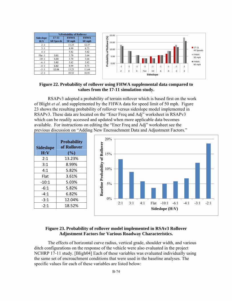
B-74

Figure 22. Probability of rollover using FHWA supplemental data compared to

values from the 17-11 simulation study.

RSAPv3 adopted a probability of terrain rollover which is based first on the work of Blight et al. and supplemented by the FHWA data for speed limit of 50 mph. Figure 23 shows the resulting probability of rollover versus sideslope model implemented in RSAPv3. These data are located on the “Encr Freq and Adj” worksheet in RSAPv3 which can be readily accessed and updated when more applicable data becomes available. For instructions on editing the “Encr Freq and Adj” worksheet see the previous discussion on “Adding New Encroachment Data and Adjustment Factors.”

Sideslope H:V

Probability of Rollover

 

 

(%) 2:1  13.23% 

3:1  8.99% 

4:1  5.82% 

Flat  3.61% 

‐10:1  5.03% 

‐6:1  5.82% 

‐4:1  6.82% 

‐3:1  12.04% 

‐2:1  18.52% 

Figure 23. Probability of rollover model implemented in RSAv3 Rollover Adjustment Factors for Various Roadway Characteristics.

The effects of horizontal curve radius, vertical grade, shoulder width, and various ditch configurations on the response of the vehicle were also evaluated in the project NCHRP 17-11 study. [Bligh04] Each of these variables was evaluated individually using the same set of encroachment conditions that were used in the baseline analyses. The specific values for each of these variables are listed below:

17-11 All Speeds

FHWA 50 mph

FHWA 60 mph

2 :1 13.23 12.373 :1 8.99 8.734 :1 5.82 5.82

Flat :1 3.61 3.70 3.64-10 :1 5.03 3.70 3.64-6 :1 5.82 5.82 5.82-4 :1 6.82 8.99 8.73-3 :1 12.04 13.23 11.64-2 :1 18.52 16.01

SideslopeH:V

%Probability of Rollover

0.00

5.00

10.00

15.00

20.00

:1 :1 :1 :1 :1 :1 :1 :1 :1

2 3 4 Flat ‐10 ‐6 ‐4 ‐3 ‐2

Probability of R

ollover (%

)

Sideslope

17‐11All Speeds

FHWA50 mph

FHWA60 mph

0%

5%

10%

15%

20%

2:1 3:1 4:1 Flat -10:1 -6:1 -4:1 -3:1 -2:1

Bas

elin

e P

rob

abil

ity

of R

ollo

ver

Sideslope (H:V)

B-75

Horizontal curve radius (1910, 955 and 637 ft) Vertical grade (-6, -3, +3, and +6 percent, downgrade and upgrade, respectively) Shoulder width (2, 6 and 12 ft) Ditch Configurations

o Foreslope width (13, 26, and 40 ft) o Ditch width (3 and 10 ft) o Backslope ratio (6:1, 4:1 and 2.5:1) o Backslope width (20 and 40 ft)

The probability of rollover as a function of combined sideslope and horizontal urve radius, as determined in the 17-11 simulation study is shown in Figure 24

Figure 24. Probability of rollover as a function of sideslope and horizontal curve radius [Bligh04]

Using the values for a tangent segment as the base condition, adjustment factors at each sideslope were determined for the three horizontal curve radii, as shown in Figure 25.

Figure 25. Adjustment factor for baseline probability of rollover as a function of

sideslope and horizontal curve radius.

Likewise, the probability of rollover as a function of sideslope and vertical grade, as determined in the NCHRP 17-11simulation study is shown in Figure 26. Adjustment

Tangent 1,910 ft 955 ft 637 ft

Flat 3.61 3.91 4.26 4.53

10:1 5.03 5.07 5.35 4.82

6:1 5.82 6.18 5.5 4.93

4:1 6.82 8.86 9.86 9.22

3:1 12.04 14.59 13.78 12.79

SideSlopeRadius of Horizontal Curve

0

2

4

6

8

10

12

14

16

Flat 10:1 6:1 4:1 3:1

P(R|slope, Hor. Curve) 

Sideslope

Tangent

1,910 ft

955 ft

637 ft

Baseline 1,910 ft 955 ft 637 ft

Flat 1 1.08 1.18 1.25

10:1 1 1.01 1.06 0.96

6:1 1 1.06 0.95 0.85

4:1 1 1.30 1.45 1.35

3:1 1 1.21 1.14 1.06

SideSlopeRadius of Horizontal Curve

0

0.2

0.4

0.6

0.8

1

1.2

1.4

1.6

Flat 10:1 6:1 4:1 3:1

Adjustment Factor for Hor. Curve 

Sideslope

1,910 ft

955 ft

637 ft

B-76

factors for each sideslope were determined for vertical grade values with zero percent grade as the base condition, as shown in Figure 27.

Figure 26. Probability of rollover as a function of sideslope and vertical grade.

[Bligh04]

Figure 27. Adjustment factor for baseline probability of rollover as a function of

sideslope and vertical grade.

These data are also located on the “Encr Freq and Adj” worksheet in RSAPv3 which can be readily accessed and updated when more applicable data becomes available. For instructions on editing the “Encr Freq and Adj” worksheet see the previous discussion on “Adding New Encroachment Data and Adjustment Factors.”

Rollover Model The probability of a terrain-related rollover for a given trajectory path is modeled

in RSAPv3 using the following relationship, which is based on the average probability of rollover as the vehicle traverses multiple sideslopes along its trajectory path: 1

| ∗ , ∗ , ∗ (7)

Where: P R Probabilityofrolloverforthetrajectory

0% ‐6% ‐3% 3% 6%

Flat 3.61 5.43 4.03 2.61 2.28

10:1 5.03 5.78 5.38 3.6 2.74

6:1 5.82 9.18 6.32 5.57 4.42

4:1 6.82 12.16 10.42 6.89 5.45

3:1 12.04 15.61 15.59 7.91 7.44

SideSlopeVertical Grade

0

2

4

6

8

10

12

14

16

18

Flat 10:1 6:1 4:1 3:1

Adjustment Factor for Grade 

Sideslope

0%

‐6%

‐3%

3%

6%

Baseline ‐6% ‐3% 3% 6%

Flat 1 1.50 1.12 0.72 0.63

10:1 1 1.15 1.07 0.72 0.54

6:1 1 1.58 1.09 0.96 0.76

4:1 1 1.78 1.53 1.01 0.80

3:1 1 1.30 1.29 0.66 0.62

SideSlopeVertical Grade

0

0.2

0.4

0.6

0.8

1

1.2

1.4

1.6

1.8

2

Flat 10:1 6:1 4:1 3:1

Adjustment Factor for Grade 

Sideslope

‐6%

‐3%

3%

6%

B-77

P R|slope Probabilityofrolloverbasedonthesideslopeatincrementiϕ , Adjustmentfactorforverticalgradeandsideslopeatincrementiϕ , Adjustmentfactorforhor.curveradiusandsideslopeatincrementiL LengthofcurrentincrementL TotallengthofthetrajectorypathN Totalnumberofincrementsalongtrajectorypathduringanalysis

The probability of rollover at each increment is weighted based on the incremental length of the trajectory, Li, as a percentage of the total length of the trajectory path, Ltot.

When the sideslope is not equal to the values in the probability table (refer to Figure 22), the probability of rollover is determined using linear interpolation. For example, for a 5:1 slope the probability of rollover would be 6.21% based on a linear interpolation between the values for a 4:1 slope and a 6:1 slope. The adjustment factors for horizontal curve radius and vertical grade are then determined using bi-linear interpolation of the corresponding adjustment factor tables based on the following relationship:

, ∗

∗

∗

∗

(8)

Where, for example, Φ11 is the adjustment factor for slope S1 and grade G1; Φ12 is the adjustment factor for slope S1 and grade G2; Φ21 is the adjustment factor for slope S2 and

. . . G1 g G2 . . .

. . .

. . .

. . .

S1 . . . ϕ11 ϕ12 . . .

s ϕsg

S2 . . . ϕ21 ϕ22 . . .

. . .

. . .

. . .

Vertical Grade

Sideslope

B-78

grade G1; Φ22 is the adjustment factor for slope S2 and grade G2; and Φsg is the unknown adjustment factor at sideslope s and vertical grade g bounded by S1, S2, G1 and G2.

Example As an example, assume that the project involves a section of roadway with a

horizontal curve radius of 1,200 ft and a vertical grade of 4%. To simplify the calculations in the rollover model, it will be assumed that the sideslope is constant at 5:1, which results in , and , having a constant value at each increment.

Determining Rollover Adjustment Factors

From the table in Figure 25 the adjustment factor for horizontal curve radius can be determined using the bi-linear interpolation function. In this case, s = 0.2 (i.e., sideslope = 5:1), g = 1,200 (i.e., horizontal curve radius) and G1 = 1,910, G2 = 955, S1 = 0.1667 and S2 = 0.25, Φ11 = 1.06, Φ12 = 0.95, Φ21 = 1.30, and Φ22 = 1.45. Using the interpolation equation yields the adjustment factor for horizontal curve, , = 1.15.

Likewise, the adjustment factor for vertical grade is determined using the interpolation equation with data from the table in Figure 26. The resulting adjustment factor, , , is 0.912. Computing Probability of Rollover

The baseline probability of rollover for a sideslope of 5:1 is 6.21%, determined from the table in Figure 23 using linear interpolation. For this simple example, it will be assumed that a given trajectory has a length of 200 feet. Noting that the rollover adjustment factors defined above are constant at each increment and that the baseline probability of rollover is constant at each increment, then from Equation (7) the probability of rollover computed as:

∑

200| ∗ , ∗ ,

∑

2006.21% ∗ 0.912 ∗ 1.15

6.51 ∗∑200

Where ∑ L is the distance that the vehicle travels along the trajectory path until it impacts a hazard. Thus, the probability of rollover in this example is equal to 6.51% for cases when the trajectory path does not encounter any hazards; and the probability decreases for cases where the trajectory distance is shortened due to impact with hazards. That is, the probability of rollover is equal to 6.51% times the ratio of the distance to the hazard along the trajectory path divided by the total length of the trajectory path (e.g., 200ft in this example).

Summary There are many variables that may affect the probability of terrain rollovers,

several of which were investigated in NCHRP Project 17-11.[Bligh04] Other variables, such as driver behavior, speed, vehicle response characteristics, soil properties, terrain imperfections, to name a few, are not very well understood. Further, the influence that each of these variables have on each other is not well understood. The rollover probability model defined above is, therefore, considered only a first approximation. The

B-79

model considers the influence of only four variables (i.e., roadside slope, highway grade, horizontal curve radius, and trajectory length), and it further assumes that the influences of these variables are independent of each other.

For example, in the 1997 “Synthesis of Rollover Research” it was shown that 85 percent vehicles overturned within a clear zone 30 ft and that only 3.5% of all rollovers were initiated on shoulders.[Mohamedshah97] It was also found that the probability of rollover was a function of ditch depth. According to Mohamedshah and Council:

“The likelihood of rollover increases with the steepness and height of sideslopes and the depth of ditches. Available data show that rollover frequency increases sharply for fill/ditch heights/depths greater than 3 ft. For example the percentage of rollovers was 12.5% for 3 feet deep ditches versus 25.1% for 4-5 feet deep ditch. Similarly the percentage of rollovers was 19.1% for 3 feet fills versus 27.2% for 4-5 feet fill.”[Mohamedshah97] Another consideration is the probability of rollover as a function of percent slope

change. For example, going from a negative slope to a less negative slope or to a positive slope would likely encourage vehicle trip.

To facilitate updating the rollover model, the rollover adjustment factors are implemented in RSAPv3 in a series of data tables which may be easily updated as additional research is conducted. The adjustment factor tables are provided on the “Encr Freq and Adj” worksheet in RSAPv3. Further, the formulation of the rollover model makes it very easy to incorporate additional adjustments factors corresponding to other variables (e.g., speed, vehicle type, and ditch depth) when they become available.

HAZARD PENETRATION Hazard penetration in this context simply means that the vehicle has gotten to the

other side of the hazard by means of structural failure of the hazard, vaulting over the hazard, or rolling over the top of the hazard. Each type of hazard “performs” in particular ways. For point hazards, there are two possible outcomes:

1. The vehicle penetrates the hazard due to structural failure (e.g., breakaway slip-base of a sign support or fracturing a wooden utility pole) or

2. The vehicle is stopped in contact with the hazard. Redirection from point hazards is not considered in RSAPv3. Determining if

structural failure of point hazards occurs is simply a matter of comparing the kinetic energy of the simulated collision with the maximum strain energy of the point hazard. For example, a 2000-lb vehicle striking a pole at 30 mi/hr has 60 ft-kips of kinetic energy. If the size of the pole indicates it has less than 60 ft-kips of strain energy capacity, the pole will breakaway; if it has more than 60 ft-kips of capacity then it will stop the vehicle without breaking away. This approach assumes that the yield force of the hazard is less than the crush force of the vehicle and that that failure does not occur until the ultimate strain energy of the hazard has been expended.

Line hazards present a more complicated situation. For line hazards there are six possible outcomes when a collision occurs:

1. Stop in contact with hazard (e.g., 90-degree impact), 2. Redirection, 3. Redirection with rollover (i.e., the vehicle rolls over on the impact side of hazard),

B-80

4. Structural failure (i.e., the vehicle goes through the hazard causing structural failure of the barrier),

5. Rollover hazard (i.e., the vehicle rolls over the barrier and lands on the non-impact side) or

6. Vaulting (i.e., the vehicle is vaulted into the air and over the hazard and lands on the non-impact side). Accounting for each of these six possible performance types is important because

each is associated with a different severity. Redirection, for example, is the preferred performance outcome for most safety barriers whereas the other outcomes are considered failures according to Report 350 and MASH because they are generally associated with higher severity crashes. If a vehicle penetrates, vaults, or rolls over a bridge railing on an overpass, for example, it may fall onto the roadway below. Rollover and vaulting are also often associated with vehicle occupant ejection which is always more hazardous than when the occupant is retained in the vehicle. In order for a vehicle to be completely stopped by a line hazard (i.e., no penetration or redirection) would require that the impact angle be near 90 degrees or that a severe snag occur between the vehicle and barrier, both of which are associated with relatively high vehicle decelerations.

Regarding increase in crash costs associated with penetrations, Sicking reported that collisions resulting in the vehicle rolling over or vaulting the barrier were more than twice as severe as those cases where the vehicle did not rollover or vault the barrier. Instead of assigning a higher “blanket” severity to such collisions, the increase in crash costs associated with penetrations is accounted for RSAPv3 as the collective sum of all collisions resulting from a given encroachment. That is, if a vehicle penetrates a barrier and then encounters a second hazard (e.g., median edge, bridge drop-off, tree-line, etc.), each incident is analyzed separately and the total crash cost for the encroachment is the sum of the all associated collision events. However, depending on the given trajectory path, secondary collisions may not occur, or there may be cases where secondary collisions occur but at very low speeds. In those cases, the penetration would have little or no effect on the overall crash cost of the encroachment.

The following sections discuss the methodology used in RSAPv3 to determine the probability of penetration due to structural failure of hazard, vaulting over the hazard, and rolling over the top of the hazard. Each section first provides background information related to the various historical methods for predicting penetration of features, followed by the methodology developed and implemented into RSAPv3 for determining probability of penetration.

Structural Penetration of Hazards

Background A variety of approaches for predicting penetration of features have been used in past

roadside safety cost-benefit analyses. BCAP, a program developed to do benefit-cost in the selection of bridge railings in the 1980’s, used a mechanistic approach to predict penetration and rollover in truck crashes; the ABC program, an updated version of BCAP, introduced improved equations for penetration; while RSAP 2.0.3 used impact severity (IS) to help predict penetrations. In all of these cases, a simple equation for predicting penetration was used and compared to some critical value. There are two main difficulties with these types of mechanistic approaches: (1) vehicle dynamics are complicated and not easily reduced to one

B-81

simple equation and (2) the capacity of a barrier is typically not known since tests-to-failure are seldom performed. For these reasons mechanistic methods have not worked particularly well.

An alternative approach is to use the statistics of real-world crashes. The advantage of a statistical approach is that a complete understanding of the physics of the problem is not required since the data represents real events. The disadvantage is that such methods require that there be crash data available in sufficient quantities in order to develop meaningful statistical models.

Mechanistic Methods

BCAP was a cost-benefit program that was developed to aid in the selection of bridge railings. BCAP was the basis for the guidelines published in the 1989 AASHTO Guide Specification for Bridge Railings (GSBR).[AASHTO89] BCAP estimates the force imposed on the bridge railing by each simulated collision using the estimated speed, angle and mass of the encroaching vehicle. This force estimate is then compared to the assumed capacity of the bridge railing. If the capacity is less than the impact force, the bridge rail is assumed to be completely penetrated and the vehicle is assumed to fall off the bridge. If the impact force is less than the capacity, redirection is assumed and the vehicle conditions are checked to see if rollover is likely.

The structural penetration model in BCAP is based on work by Olson in NCHRP Report 149. [Olson74] Olson suggested that the lateral force imparted by the vehicle to the barrier could be approximated as:

2 sin 2 1 cos

(9)

Where: Flat = The average lateral deceleration of the vehicle, W = The weight of the vehicle in lbs, V = The vehicle impact velocity in ft/sec, Θ = The impact angle, A = The distance from the front of the vehicle to the center of mass in ft,

B = Vehicle width in feet and D = Lateral deflection of the barrier in feet.

BCAP randomly generates a set of encroachment conditions (i.e., speed, angle and vehicle type) and the lateral force can then be calculated based on those assumed impact conditions. If the lateral impact force is greater than the capacity of a barrier, the barrier is assumed to have failed structurally.

While Olson’s model is a good simple estimator it certainly has its limits. First, it is based on estimating the impact force but damage and failure is more properly related to strain energy. Unfortunately, while impact energy is easy to calculate (i.e., ½ mv2), the strain energy capacity of a barrier is quite difficult to calculate at least in some simplified general form. Also, in developing the 1989 GSBR recommendations, it was assumed that the barrier deflection would always be zero (i.e., the D term in the equation above) but for longitudinal barriers in general, the deflection is also a function of the impact

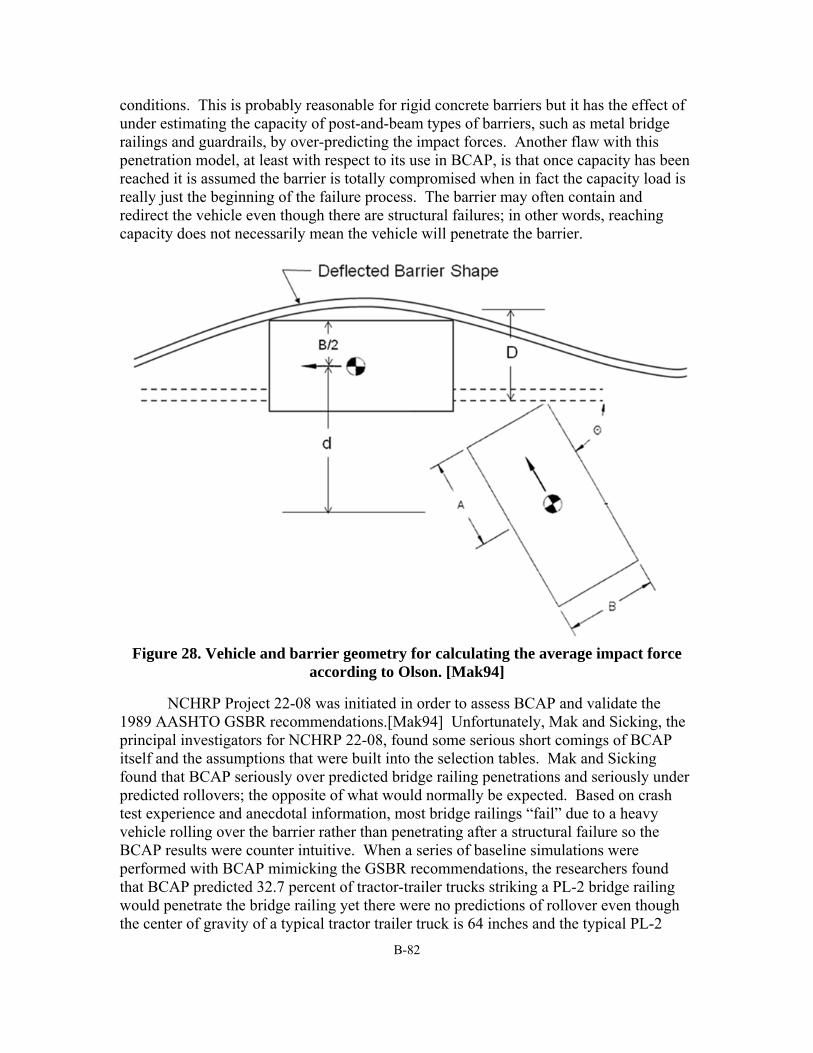
B-82

conditions. This is probably reasonable for rigid concrete barriers but it has the effect of under estimating the capacity of post-and-beam types of barriers, such as metal bridge railings and guardrails, by over-predicting the impact forces. Another flaw with this penetration model, at least with respect to its use in BCAP, is that once capacity has been reached it is assumed the barrier is totally compromised when in fact the capacity load is really just the beginning of the failure process. The barrier may often contain and redirect the vehicle even though there are structural failures; in other words, reaching capacity does not necessarily mean the vehicle will penetrate the barrier.

Figure 28. Vehicle and barrier geometry for calculating the average impact force

according to Olson. [Mak94]

NCHRP Project 22-08 was initiated in order to assess BCAP and validate the 1989 AASHTO GSBR recommendations.[Mak94] Unfortunately, Mak and Sicking, the principal investigators for NCHRP 22-08, found some serious short comings of BCAP itself and the assumptions that were built into the selection tables. Mak and Sicking found that BCAP seriously over predicted bridge railing penetrations and seriously under predicted rollovers; the opposite of what would normally be expected. Based on crash test experience and anecdotal information, most bridge railings “fail” due to a heavy vehicle rolling over the barrier rather than penetrating after a structural failure so the BCAP results were counter intuitive. When a series of baseline simulations were performed with BCAP mimicking the GSBR recommendations, the researchers found that BCAP predicted 32.7 percent of tractor-trailer trucks striking a PL-2 bridge railing would penetrate the bridge railing yet there were no predictions of rollover even though the center of gravity of a typical tractor trailer truck is 64 inches and the typical PL-2

B-83

barrier height was 32 inches (i.e., the c.g. of the vehicle is 32 inches higher than the top of the barrier). [Mak94] Mak and Sicking discovered several reasons for this. One reason was the algorithm used to predict rollovers resulted in unreasonably high critical velocities. A new rollover algorithm was proposed and implemented as will be discussed in the next section.

Another reason involved barrier capacity. BCAP estimates the forces on the barrier using the Olson equation shown above. The equation is a simple derivation of the force based on the overall mechanics of the impact. The force in Olson’s equation is actually the average lateral force required to arrest (or redirect) the lateral component of kinetic energy (i.e., kinetic energy due to the lateral component of velocity) of the vehicle during redirection and can be derived based on the energy balance equation:

∗12

(10)

Where in Olson’s equation the lateral component of kinetic energy is given as, 1

212

(11)

Olson’s equation neglects energy loss due to frictional forces (e.g., friction between the vehicle and barrier and friction between the vehicle tires and ground), plastic deformation of the vehicle, as well as energy converted to angular rotational energy (i.e., arising from pitch and roll angular velocities).

The d term in Equation (10) is the distance through which the force moves to absorb/transform the kinetic energy. It is assumed that the vehicle rotates about the center of gravity (c.g.) of the vehicle; thus, d is the total distance that the c.g. moves toward the barrier during redirection (i.e., from time of impact until the vehicle has become parallel to the barrier). This distance is defined as:

sin2 2

where, as shown Figure 28:

sin is the lateral distance from the c.g. of the vehicle to the face

of the barrier

is the width of the vehicle and

is the deflection of the barrier The calculated impact force is then compared to the theoretical bridge rail

capacity. If the impact force is greater than the capacity, the bridge rail is considered failed. Estimating the actual capacity of bridge railings is more difficult than it might first seem. Materials are routinely assumed to be less strong and loads are routinely over estimated in design so even if the theoretical capacity is calculated it is likely a conservative value. For example, in designing concrete structures a resistance factor 0.85 is usually used for bending which essentially takes advantage of only 85 percent of the strength of concrete. Likewise, if an allowable stress design method for steel were used, 67 percent of the strength of the steel is assumed. In both cases, the designer is neglecting a significant portion of the capacity of the structure.

While this makes excellent design sense, it makes it difficult to estimate the real failure conditions of the structure. BCAP assumed that PL-1 bridge railings have a

B-84

capacity of 15 kips, PL-2 railings have 35 kips and PL-3 railings have 55 kips. While there are relatively few crash tests where structural failure of the bridge railing was observed, Mak and Sicking were able to find some cases where the bridge railing experienced some degree of structural failure (i.e., hairline cracking, spalling, etc.). When they compared the limited crash test results to the BCAP assumptions they found that the BCAP assumptions were about half what could be supported by crash tests as shown in Table 21.

Table 21. Bridge railing capacity recommendations in BCAP and NCHRP 22-08.[after Mak94]

Performance Level BCAP Assumption (kips)

Mak/Sicking Recommendation

(kips) PL-1 15 30 PL-2 35 64 PL-3 55 108

Adding to the difficulty is the basic assumption in BCAP that when capacity is reached, the bridge railing will totally fail and allow the vehicle to penetrate. In fact, this does not generally happen. Bridge railings can experience structural failure and sometimes will still redirect the vehicle. The failure may be cracks or spalls that, while considered serious structural damage, do not result in a complete loss of structural capacity.

Recently, Alberson and others evaluated a 32-inch high PL-2 concrete safety shaped barrier that had experienced structural failure problems in the field as shown in Figure 29. [Alberson11; Alberson04] A yield-line structural analysis was performed on the bridge railing which resulted in an estimated barrier capacity of 41.46 kips when loaded near a construction joint and 62.09 kips when loaded at the mid-span. The same design was then constructed and statically tested to failure resulting in a near-the-joint capacity of 35.1 kips, a capacity at the expansion joint of 45.1 kips, and a mid-span capacity of 73.1 kips.

Figure 29. Damage to a 32” concrete bridge railing in a crash with a single unit

truck in Florida. [Alberson04]

B-85

The bridge railing was also subjected to full-scale Report 350 TL-4 crash tests which were passed successfully and which caused relatively minor concrete damage (e.g., hairline cracks and some gouging). As shown by Alberson’s research, the capacity values suggested by the 1989 AASHTO GSBR were grossly over conservative and those proposed by Mak and Sicking were much more appropriate although it should be noted that this particular railing was chosen for investigation precisely because there had been some observed field structural failures, so this particular railing probably represents the lower end of the capacity of PL-2 railings. Since BCAP first assesses the capacity and then the rollover potential, the overly conservative values for capacity tended to over predict penetrations for trucks and under predict trucks rolling over the barrier.

Mak and Sicking revised the rollover algorithm, which will be discussed later in the Roll-Over-Hazard section, and adjusted the bridge railing capacities upward as shown in Table 21 and re-ran their analysis. In the initial BCAP runs, 32.7 percent of tractor trailer truck crashes penetrated the railing and none rolled over whereas after the improvements implemented by Mak and Sicking were made 1.2 percent penetrated and 8.9 rolled over which seemed more reasonable.

Mak and Sicking also evaluated bridge railing crash data from Texas to determine field-based penetration and rollover rates. [Mak94] Mak and Sicking found that the Texas data indicated that 2.2 percent of bridge railing crashes result in the vehicle going through (i.e., penetration) or over (i.e., roll over the barrier) and they believed that even this value was a high-side estimate due to coding errors on the police crash reports. The improved BCAP with the higher capacity limits and improved rollover algorithm resulted in an overall estimate of 10 percent going through (i.e., 1.2 percent penetrating and 8.9 percent rolling over) for the typical Texas conditions so even the improved BCAP appeared to over predict penetrations/rollover by an order of magnitude although the proportion of penetrations to rollovers appears much more reasonable.

In summary, then, BCAP and the 1989 AASHTO GSBR appear to greatly over predict bridge railing penetrations and under predict rollovers. The improvements from NCHRP 22-08 appeared to improve the results considerably although even the improved BCAP over predicts the incidence of vehicles going through or over the bridge railing.

RSAP versions 2.0.3 and before include two sets of procedures to deal with vehicle penetration of features and rollover after hitting features. For example, RSAP 2.0.3 first identifies whether an impacting vehicle would be likely to penetrate the first-struck hazard. For point hazards like breakaway objects, such as trees, wooden utility poles, and breakaway supports (i.e., Type 5 Fixed Objects Features in RSAP 2.0.3), the penetration is predicted if the impacting vehicle is above a threshold value of kinetic energy calculated as: 1

2 (12)

where KE = Kinetic energy of impacting vehicle (joules=kg*(m/s)2) m = Mass of impacting vehicles (kg) V = Impact speed (m/s)

B-86

Similarly, longitudinal barriers (RSAP Type 7 Features) are predicted to be penetrated when the impact severity (IS) of an impact is higher than the containment limit for the barrier test level. The IS value is calculated as: 1

2sin (13)

where IS = Impact severity m = Mass of impacting vehicles (kg) V = Impact speed (m/s) = Impact angle (deg) If hazard penetration is predicted, RSAP calculates the energy gained or lost in

impacts with roadside features that are penetrated. For roadside features other than side-slopes, the energy associated with the capacity or containment limit of the feature is subtracted from the vehicle’s initial kinetic energy (or its lateral component in the case of a guardrail). A new speed for the vehicle is then calculated on the basis of the remaining energy and this new speed is used for the next impact. A roadside slope, provided it is not very steep, would not be expected to affect the vehicle’s kinetic energy appreciably; however, the resultant rise or drop in the vehicle’s center of gravity during slope traversal would affect the vehicle’s potential energy. Thus, the potential energy associated with traversing a roadside slope is added (or subtracted if going uphill) from the initial kinetic energy of the vehicle to determine a new speed for the next impact. Further, RSAP 2.0.3 estimates the crash severity of the first feature struck as well as any subsequent features in the vehicle’s path. The highest severity of any feature in the vehicle’s path is then utilized in the calculation of crash cost.

Several recent research projects are revisiting the question of barrier capacity. Alberson’s work on a 32-inch New Jersey safety shaped bridge railing has already been discussed earlier. Bligh is currently doing work on quantifying the impact forces on TL-4 and TL-5 barriers as a part of NCHRP 22-20(2) through the use of finite element analysis.[Bligh12] Ray is currently compiling barrier strength calculations as well as crash test data for several common closed-profile concrete bridge rails for use in establishing a relationship between theoretical barrier capacity and probability of penetration as part of NCHRP 22-12(3).[Ray12]

Statistical Methods

Penetration can also be observed in the field and, depending on the form of the police reports, can sometimes be deduced from the police-level crash data. One particular example where there is a fairly large amount of data on barrier performance is low-tension cable median barriers. Several states have reported the effectiveness of cable median barriers in terms of the percentage of crashes that were contained by the barrier. If the barrier prevented the vehicle from crossing to the opposing lanes of traffic, then it was considered to be effective in containing the vehicle. Some of the data in Table 22 represents fairly limited data collection, but several of the states have been collecting cable median barrier crash data for nearly a decade and have collected over 400 cases. In general, it appears that the vehicle is prevented from crossing over into the opposing lanes of traffic in about 95 percent of the cases (i.e., about 5 percent penetrations

B-87

assuming that rollover on a cable barrier is unlikely). The states listed in Table 22 have all used cable median barriers and studied their effectiveness. In all cases, with the exception of Utah, it was found that less than seven percent of police reported crashes penetrate the barrier. The States with the most police-reported cases all show penetration rates of less than 5.3 percent. Considering the collective results of all the states, that is, the total number of penetrations divided by the total number of collisions (i.e., 162 / 6221), results in a 2.6% penetration rate.

Table 22. Performance of cable median barriers in various States. [Ray09, MacDonald07]

State Collisions Penetrations Penetrations (No.) (No.) (%)

AR 490 25 5.1 IA 20 0 0.0 NC 71 5 7.0 NY 99 4 4.0 MO 1,402 67 4.8 OH 372 4 1.1 OK 400 1 0.2 OR 53 3 5.7 RI 22 0 0.0 SC 2500 10 0.4 UT 18 2 11.1 WA 774 41 5.3

The State of Washington probably has the most complete information on cable

barrier crashes and has performed assessments of low-tension cable median barrier, high-tension cable median barrier and concrete safety shaped median barrier performance in 2007 through 2009. [MacDonald07, Hammond08, Hammond09] As summarized in Table 23, six percent of low-tension cable median barriers allowed the vehicle to penetrate and cross the median compared to 3.7 percent for high-tension cable median barriers and 2.2 percent for concrete safety shaped median barriers. The severe and fatal injury percentage for each barrier type is also included in Table 23. Interestingly, vehicle contained in the median and those that cross the median appear to have very similar severe and fatal injury percentages. This study by Washington State, therefore, shows the penetration percentages of three different types of barriers.

B-88

Table 23. Barrier Performance in Washington State.

Barrier Performance

Low-Tension Cable

High-Tension Cable

Concrete

No. % A+K %

No. % A+K %

No. % A+K %

Contained in Median

742 85.9 1.1 560 71.5 0.9 441 34.0

Redirected 70 8.1 0.1 194 24.8 0.4 828 63.6 Crossed the Median 52 6.0 1.4 29 3.7 0.9 28 2.2 Total 864 100.0 783 100.0 1,297 100

MoDOT performed an in-service evaluation of its cable median barriers in 2005. [MoDOT06] Data analysis from 1999 to 2005 yielded 1,402 crashes involving cable median barriers. Successful performance was defined as “the vehicle does not make it to the opposing travel lanes,” whereas failure indicated that the vehicle penetrated the barrier and entered the opposing lanes. By this definition, 95.2 percent of the cable median barrier crashes were considered successful in that they prevented a cross-median event so at least 4.8 percent of the cases resulted in a barrier penetration.

Information such as that shown above could be used in RSAP to assign a particular percentage or probability of penetration for each type of barrier. Table 23 seems to indicate that about six percent of vehicles penetrate a low-tension cable median barrier, about four penetrate a high-tension cable median barrier and about two percent penetrate a concrete safety shape. Of course, a crash study like the one above would be required to determine the appropriate percentages for use in RSAP.

The cable barrier example is interesting in that the penetrations of cable barriers are seldom ever capacity related. Generally, vehicles penetrate cable barrier by going under, through or over the cables which does not load the barrier to its structural capacity. This points out that there are two types of penetration failures – capacity related failures and non-capacity related failures that are usually more associated with vehicle and barrier geometry.

Comparison of Mechanistic and Statistical Approaches

Each method for assessing the probability of barrier performance has its strengths and weakness with respect to use in RSAP as shown in Table 24. The mechanistic methods that have been used in previous cost-benefit programs use some simplified version of the equations of motion of the vehicle and the law of energy conservation to estimate the forces on barrier and vehicle. While mechanistic methods have the advantage that they are grounded in the physics of the problem, getting a simple closed-form solution usually involves making many broad assumptions about the impact which may or may not be correct. Very accurate predictions about vehicle dynamics can be obtained using finite element analysis or vehicle dynamics analysis but these require extensive input and long runtimes to develop an answer which would not be feasible in the context of RSAP where tens of thousands of simulated encroachments are needed.

B-89

Simple one-equation models like those used in BCAP and RSAP 2.0.3 simply are not adequate to capture the full range of vehicle dynamics.

Table 24. Strengths and weakness of the mechanistic and statistical approaches to

hazard penetration.

Mechanistic Statistical Strength Weakness Strength Weakness

Based on physics Capacity of barriers is seldom known a priori.

Based on real-world data and therefore likely to be accurate.

May not be data available for many types of barriers, especially new or specialty barriers.

Useful for barriers with unknown field performance.

Simple equations for prediction are not very accurate.

Easy to compute and implement in RSAP.

May not be able to determine the impact conditions most associated with performance.

Based on impact conditions and structural assessment.

Complex simulations are not practical and would be difficult to implement.

Simple equations would be easy to implement.

Another major flaw with most mechanistic penetration models is that once

capacity has been reached it is assumed that the barrier is totally compromised when in fact the capacity load is really just the beginning of the failure process. The barrier may often contain and redirect the vehicle even though there are structural failures, as was determined by Plaxico and Ray in NCHRP Project 22-12(3) in their review of 50 full-scale crash tests on concrete bridge rails and median barriers. In other words, reaching capacity does not necessarily mean the vehicle will penetrate the barrier.

Another deficiency in the existing mechanistic models is that the effect of barrier shape on vaulting over the barrier and rollover on the traffic side of the barrier by vehicles with c.g. heights lower than the barrier height is generally ignored. For example, passenger cars sometimes vault over safety shaped barriers even though the height of the passenger car c.g. is lower than the barrier height (i.e., they cannot roll over the barrier). The reason is that the shape of the barrier in some shallow angle impacts has the effect of launching the vehicle over the barrier. This is not captured in a simple one-equation mechanistic model.

The most notable advantage of a statistical approach is that a complete understanding of the physics of the problem is not required since the data represents real events. Statistics data are also relatively easy to implement or update in RSAPv3 since they listed directly in a look-up-table (LUT) on an existing RSAPv3 worksheet. The

B-90

disadvantage is that for some vehicle types and some barrier types there may not be sufficient quantities of crash data available for development of meaningful statistics data.

RSAPv3 Implementation In previous cost-benefit programs, like BCAP, ABC and RSAP 2.0.3, penetration

was determined based solely on the mechanics of the impact event. That is, the impact conditions were calculated and compared to the known structural capacity of the hazard. If impact conditions exceeded the capacity of the hazard then the hazard was assumed to be completely penetrated; otherwise the vehicle was either redirected or was stopped in contact with the hazard. However, there should not be such a drastic transition from a zero probability of penetration, when impact conditions are just below theoretical capacity, to a 100% probability of penetration, when impact conditions are exactly at capacity. There are many variables that contribute to the outcome of a crash event that cannot be accounted for in these simple calculations. It thus seems reasonable to assume that for very low impact speeds and angles the probability of penetration would be relatively low and would increase gradually as the impact conditions approach and began to exceed the capacity of the barrier.

The structural penetration model in RSAPv3 deals with penetrations using a combination of both crash statistics and the mechanics of the collision event. The penetration model, which is illustrated in Figure 30, uses two different approaches for determining penetration; the approach used for a given impact case is determined based on two sets of criteria:

Criterion A – If the impact severity is greater than the structural capacity of the barrier (i.e., IS/Capacity > 1) and the structural capacity is greater than or equal to zero, then the probability of penetration is determined based on a combination of impact mechanics and a pseudo-probabilistic model, where the probability of penetration up to capacity is based on crash statistics and increases toward 100% as impact severity values increase beyond hazard capacity.

Criterion B – Else, (i.e., If the impact severity is less than the structural capacity of the barrier or if the structural capacity of the barrier is zero or unknown), the probability of penetration is defined solely based on crash statistics (i.e., the PRV percentage tabulated for each hazard on the “Severity” worksheet in RSAPv3).

B-91

Figure 30: Probability model for structural penetration of hazards in RSAPv3

Crash statistics are considered to be more reliable for predicting crash outcomes than mechanistic approaches, but such data is generally only available in sufficient quantities for the passenger-class of vehicles (e.g., cars, pickups and SUV’s). Although there is a significant amount of crash data available related to certain kinds of point hazards such as utility poles and trees, very little, if any, of the data can be used for developing statistical models for structural penetration.[Mak80] The data in those studies generally only include information related to crash severity, such as number of occupants, occupant injury and vehicle damage. Since crash reconstruction data does not accurately distinguish between hazard penetrations caused by (1) structural failure, (2) rolling over the hazard and (3) vaulting, those events have been combined into a single variable denoted by the acronym, PRV (Penetration/Rollover the hazard/Vault). This data is generally derived from police-reported crashes as was discussed in the background section (see Table 22 and Table 23). It should be noted that the probability of penetration derived from crash statistics generally represents the average probability from all collisions and includes a large range of vehicle makes and models, as well as countless impact conditions. The authors are not aware of any studies in which statistics models have been developed for predicting penetration based on impact conditions (e.g., speed, angle, energy, IS, etc.) or vehicle type, but such models may be readily implemented into the penetration subroutine in RSAPv3 if/when such data becomes available in the future.

The penetration algorithm corresponding to Criterion B in Figure 30 is based on a hyperbolic-tangent function defined by:

|12

∗ tanh12

(14)

Where A defines the point of symmetry of the curve, B controls the slope of the curve, and s controls the lower bound value of the curve, IS is the impact severity of the

0

0.1

0.2

0.3

0.4

0.5

0.6

0.7

0.8

0.9

1

0 0.5 1 1.5 2 2.5 3

Pro

bab

ilit

y of

Pen

etra

tion

IS/Capacity

Criterion B: Penetration based on

crash statistics

Criterion A: Penetration based on Mechanistic-Statistics

model

PRV

B-92

impacting vehicle and Capacity is the strain energy capacity of the hazard. Note that the relationship between impact severity (IS) and kinetic energy (KE) is defined by: ∗ (15)

Where is the impact angle with respect to the longitudinal orientation of the hazard. In the case of point hazards, RSAPv3 sets the impact angle to 90 degrees, in which case impact severity is equivalent to kinetic energy.

The probability function shown in Figure 30 corresponds to Equation (14) with A = 1.5 and B = 5 and s = PRV. The probability model indirectly accounts for variations in crash conditions, such as vehicle properties (e.g., mass, stiffness, suspension, etc.), impact conditions (e.g., vehicle tracking orientation, angular rates, etc.) and barrier strength properties (e.g., material/mechanical properties, structural joints, etc.). The model parameters defined above result in a probability of penetration equal to PRV at IS/Capacity = 1 (i.e., creates a continuous function with respect to Criterion A) and the probability gradually increases toward a value of 1.0 as IS/Capacity approaches 2.0. These assumptions were based on engineering judgment and through calibration of RSAPv3 results during sensitivity analyses. The parameters of the model should be revised when additional penetration and or hazard capacity data becomes available. Note that the probability of PRV for each hazard type is provided on the RSAPv3 “Severity” worksheet and can be readily updated as warranted based on crash data. If the value for PRV is not defined on the “severity” worksheet, its value is set to zero.

Speed Change due to Penetration

When RSAPv3 determines that a penetration has occurred based on structural failure of the hazard (i.e., IS > Capacity), the energy lost in the impact event is calculated and the post-penetration velocity is reduced accordingly. For roadside features other than side-slopes, the energy loss is equal to the structural capacity of the feature. Thus, the structural capacity is subtracted from the vehicle’s initial kinetic energy and a new speed for the vehicle is computed, as shown in Equation (16),

2

(16)

Where vp is the post-penetration velocity of the vehicle, KE is the initial kinetic energy of the vehicle upon impact, and Capacity is strain energy capacity of the hazard.

However, a significant portion of hazard penetrations are not strictly due to structural penetration. For example, penetrations often occur due to override of w-beam guardrails, vaulting over safety shape barriers or passing between (“splitting”) cables in cable barrier systems. These types of penetrations are those that meet Criteria B in the penetration model. In many of those cases, the energy expended in the collision is relatively low, as illustrated in the full-scale crash test of the w-beam guardrail in Figure 31. The impact speed in the test was relatively low (i.e., 43.2 mph). The vehicle immediately began to vault the guardrail upon impact, experiencing little or no redirection. The exit velocity was reported to be 36.4 mph, which corresponds to a loss in kinetic energy of approximately 30%. It is assumed that this value is a conservative estimate, thus when a penetration is determined to occur based on the PRV percentage,

B-93

the velocity is reduced in RSAPv3 assuming a 30% loss of kinetic energy using the following relationship: Δ ∗ 30%

2Δ

(17)

The vehicle then continues along its original path at the new velocity and

continues to decelerate based on the original trajectory data.

Figure 31. Summary of results for TTI test 0482-1 on the G4(2W) with 12.5-ft post

spacing.[Mak93]

Theoretical Hazard Capacity The structural capacity of hazards, particularly roadside safety barriers such as

bridge rails and concrete median barriers, is often referred to in terms of ultimate load. In RSAPv3, however, barrier capacity is defined in terms of “Penetration Energy” which corresponds to the energy required to structurally fail the hazard and allow penetration.

As discussed in the background section, estimating the strength capacity of safety barriers is more difficult than it might first seem. In barrier design, the material properties of the barrier components are routinely taken as their lower bound values, while loads are routinely over estimated, so that the calculated theoretical capacity is generally a conservative value. Further, penetration is not guaranteed in real world

B-94

impacts when impact conditions are at or just beyond the threshold of hazard capacity. For example, collisions involving heavy trucks often result in impact forces and energies that exceed a barriers capacity. However, it has been shown in full-scale tests that even though the barrier suffered structural damage during impact the truck was still safely redirected. This may, in part, be due to the fact that tractor-trailer vehicles are articulated and generally result in three peak loads on the barrier corresponding to 1) initial impact of the tractor against the barrier, 2) simultaneous impact of the rear tandem axles and front of trailer against the barrier and 3) impact of the trailer axles against the barrier.

Note that the calculation of IS basically assumes that the total mass of the vehicle is concentrated at the point of impact and does not account for the relationship between the stiffness of the structure and the distribution of mass along its length which effectively overestimates the loads imparted to the barrier. This is particularly true for articulated vehicles where the impact is distributed over three separate peak loadings and the magnitude of these peak loads are further affected by kinematic response of the vehicle; for example, tractor-trailer vehicles tend to roll over on top of the barrier during redirection which reduces the lateral impact forces imparted to the barrier. Also, the highest load is often associated with the impact of the trailer axles; however, the momentum of the vehicle moving along the length of the barrier tends to pull the trailer away from the damaged region and penetration is, thereby, avoided. In such cases, an accurate characterization would require a multi-degree of freedom representation of the vehicle which would be too computationally demanding for use in RSAP which evaluates tens of thousands of encroachments.

Since different classes of vehicles tend to interact differently with longitudinal barriers, RSAP results could be improved if the probability of penetration was based on vehicle class (e.g., passenger vehicles, light trucks, tractor-trailer, etc.) and impact conditions (e.g., IS). An important task in another ongoing NCHRP project (i.e., Project 22-12(3)) is to collect barrier capacity data for closed-profile concrete bridge rails and to establish the likelihood of barrier penetration in collisions based on impact conditions (e.g., mass, velocity, impact angle), barrier height and test level. That task is still underway and final results and conclusions are not yet available although it is likely they will be incorporated into a later release of RSAPv3.[Ray12]

Hazard capacity is listed on the “Severity” worksheet in RSAPv3 and can be readily updated as discussed later in the Crash Severity Module. When capacity data is unknown, its value should be left blank on the worksheet, in which case RSAPv3 will use PRV data to determine hazard penetrations (i.e., Criterion B).

Roll-Over-Hazard Penetrations

Background BCAP also included a rollover algorithm to predict if trucks would roll over the bridge railings. The rollover algorithm was only activated in BCAP when the bridge railing was not penetrated. BCAP first checks to see if the penetration capacity has been reached. If capacity has been exceeded, the vehicle penetrates the railing. If capacity has not been exceeded, the vehicle is assumed to be redirected and the roll-over-barrier algorithm is checked. The roll-over-barrier condition in the original BCAP is:

B-95

(18)

Where: Vcr = The velocity in ft/sec that the vehicle would roll over the barrier, B = The width of the vehicle in feet

g = The acceleration due to gravity (i.e., 32.2 ft/s2), Hcg = The height of the vehicle center of gravity in inches, Hb = The height of the barrier in inches and

Θ = The impact angle in degrees. This formulation assumes that the vehicle forces act at the center of gravity of the

vehicle and that the barrier forces act at the very top of the barrier. Mak and Sicking reviewed BCAP’s roll-over-barrier algorithm in project 22-08.

They found that this equation yields critical velocity estimates that are much too high so BCAP seldom predicted a rollover. Mak and Sicking modified the model by assuming the barrier forces act at the vehicle axle rather than top of the barrier and that the truck would rotate about the top of the barrier when the truck deck settled onto it during the rollover. The improved impulse-momentum model is given by:

(19)

Where the terms are as defined before with the addition of: d = Distance from the vehicle c.g. to the bottom edge of the truck frame in inches, Hf = Height of the center of the truck axle in inches, R = The radius of gyration of the truck and its load about the bottom corner of the truck

frame in units of feet, and is defined by:

0.454 144

(20)

This model was validated to some extent with HVOSM and NARD and resulted in lower critical velocities and more rollovers in the BCAP analyses which was the objective. The improved rollover algorithm and adjustments to the barrier capacity performed by Mak and Sicking greatly improved the estimates of BCAP but BCAP still predicted more crashes than comparison to the real-world data available at the time indicated.

In both models, however, the effect of barrier shape on vaulting over the barrier by vehicles with c.g. heights lower than the barrier height is ignored. For example, many passenger cars vault over barriers even though the center of gravity of the vehicle is lower than the barrier height. The reason is that the shape of the barrier in some shallow angle impacts has the effect of launching the vehicle over the barrier.

B-96

RSAPv3 Implementation It is assumed that passenger vehicles are not likely to rollover hazards; and the small percentage that do is indirectly accounted for in the structural penetration algorithm via the PRV statistics. For trucks, on the other hand, sufficient crash data is not currently available for developing meaningful statistics. In the case of trucks, RSAPv3 includes a somewhat simple algorithm based on impulse-momentum principles to predict if trucks will roll over longitudinal hazards, such as guardrail, median barriers and bridge rails, during collisions. The development of this model was based largely on the work of Labra, et al. [Labra76] The rollover algorithm is only activated for the analysis of truck trajectories and only when the center-of-gravity of the truck is higher than the top of the hazard.

In the hazard penetration module, RSAPv3 first determines the probability of structural penetration (e.g., penetration based on impact energy and hazard capacity). Then, if the vehicle is a truck, the next step is to determine the probability of the truck rolling over the hazard.

When a truck rolls over a barrier there are two possible outcomes: (1) truck simply rolls over the barrier and stops or (2) a secondary collision occurs, such as falling off of a bridge or impact with another hazard. Note that both outcomes involve a rollover event. However, RSAPv3 does not consider this type of rollover as a separate collision. RSAPv3 simply sees it as a penetration and checks for subsequent collisions from the post-penetration trajectory that would add to the crash cost (e.g., fall off an overpass, strike another hazard, etc.). It was assumed that the cost of a rollover event together with the cost of a subsequent collision would overestimate crash costs and that the cost of rolling over the barrier should only be based on the initial collision and on what the vehicle struck as a result of penetrating behind the barrier. The potential for rolling over a barrier is obviously dependent on the impact conditions of the encroaching vehicle as well as the barrier’s dimensions. The following sections describe the development of a simple algorithm for calculating potential rollover-vault of a light truck impacting against rigid longitudinal barriers using elementary principles of impulse and momentum. It was of key interest to ensure that the rollover prediction model did not compromise the efficiency of RSAP when evaluating crash statistics; thus the goal was to develop an algorithm accurate enough to provide reliable results with minimal computations. Methodology

A rollover-vaulting algorithm was developed based on a four-phase analysis of the rollover event:

Phase 1: Initial impact between the front-corner of the truck against the barrier is evaluated using simple three-dimensional angular impulse-momentum principles to determine kinematics of the truck immediately after initial impact.

Phase 2: Motion of the truck is then evaluated assuming that the front corner of the truck remains in contact with the barrier as the vehicle yaws toward the barrier. From this analysis the translational and angular velocities and displacements are determined at the point when the vehicle is parallel to the barrier.

B-97

Phase 3: As the vehicle yaws toward the barrier, a second impact event occurs when the side of the truck impacts against the barrier. This phase of the event is evaluated using impulse-momentum principles to determine the resulting kinematics of the truck related to rolling toward the barrier.

Phase 4: The final phase of the analysis involves applying the principle of conservation of energy to determine if the resulting kinematics of the truck are sufficient to allow the vehicle to rollover/vault the barrier. The analysis procedure considered here is based on elementary principles and is

carried out using broad assumptions about the impact event in order to simplify the analysis and ultimately to reduce the computational effort. A notable omission of this model is the effects of friction between the truck and barrier as well as the effects of friction between the tires and ground. These forces would have the most influence in phase 2 and phase 4 of the analysis procedure, which are the non-impulsive analyses, where the motion of the vehicle is governed by: (1) the translational and angular velocities resulting from the impulsive forces generated in Phase 1 and Phase 3, (2) the constraint of the barrier, and (3) the frictional forces as the vehicle interacts with the barrier and ground.

Additional omissions of this model include the vehicle suspension and vehicle deformations (e.g., elastic and plastic deformations). The vehicle is thus assumed to move as a rigid body. Further, the barrier is assumed to be rigid, flat, smooth and vertical; that is, barrier deflections, barrier component deformations, vehicle “snag” on barrier, etc. are ignored. Nonetheless, these calculations do, in general, provide a reasonably conservative estimate of the potential for rolling over the barrier.

Phase 1 of Impact

The initial phase of impact involves the vehicle impacting the face of the barrier under “tracking” conditions at speed, vx0, and impact angle, ψ0. All other translational and rotational displacements and velocities are assumed to be zero during this phase. The analysis procedure for this initial impulsive phase was adopted from Labra, et.al and is repeated here for convenience.[Labra76]

The analysis is carried out based on a vehicle fixed reference frame (x, y) and an inertial reference frame (x′, y′), as illustrated in Figure 32. Upon impact with the barrier, the resulting kinematics of the vehicle can be approximated by applying the angular momentum principle about the center of gravity (c.g.) of the vehicle. The angular velocities ωx, ωy and ωz about their respective vehicle fixed reference frame are defined by the following relationship:

∗ x (21)

Where, thevehicle smomentofinertiaaboutitscenterofgravitythemomentarmfromthec. g. totheimpactpointOonthebarrierimpulsiveforcesbetweenthevehicleandbarrier

B-98

Figure 32. Schematic drawing of vehicle impacting barrier.

Applying the linear-momentum principle at impact yields: ∗ (22) Where,

Massofvehiclevelocityvectorimediatelyafterimpactvelocityvectorbeforeimpactimpulsiveforceassumedtoactinthenegativevehiclefixedreferenceframe

Assuming that impulsive forces arising from friction between the vehicle and

barrier can be ignored, then it follows that the forces in the plane of the barrier are zero, which leads to: cos sin 0

0 (23)

Where is the initial yaw angle between the vehicle and the barrier. The velocity of the vehicle center of gravity with respect to the velocity of the vehicle at contact point O is defined by: x / (24) Where,

componentsofvelocityatcontactpointO

B-99

/ distancevectorfromcontactpointOtothec. g. refertoFigure1

Expanding Equation (24) yields,

(25)

Assuming that the vehicle remains in contact with the barrier at point O during this phase, then the velocity at Point O in the inertial reference frame (i.e., x’, y’, z’) 0 (26) If we define as the impulse force acting normal to the barrier in the inertial coordinate frame, then we have: sin cos (27) And

x

∗ ∗ cos∗ ∗ sin

∗ sin ∗

(28)

Substituting Equation (27) into Equation (21) and expanding yields, ∗ ∗ cos

∗ ∗ sinsin

(29)

Rewriting Equation (22) using the relationships defined in Equation (27) yields sin

cos0

(30)

Combining Equations (24), (25) and (26) and noting that the roll and pitch angles at impact are zero yields, v sin cos 0 (31) Substituting Equations (25) into Equation (31) results in, cos sin cos sin

sin cos 0 (32)

Equations (29), (30) and (32) yield seven equations for solving the seven unknowns: ωx, ωy, ωz, , , , and .

Phase 2 of Impact

Phase 2 involves redirection of the truck where the motion during redirection is a function of the post-impact kinematics of the vehicle (i.e., defined in phase 1) and by the frictional forces arising from contact between the truck and barrier and those between the

B-100

tires and ground. In order to properly characterize the vehicle’s motion during this important phase of the impact would require solution of the non-linear equations of motion via a numerical integration, which would require substantial computational effort given the application of this algorithm (i.e., implementation in RSAP). However, making the simplifying assumption that the effects of friction can be neglected and assuming that the vehicle moves as a rigid body, then the motion of the vehicle can be approximated based on its post impact kinematics.

Assuming that point O on the vehicle remains in contact with the barrier and slides along the top of the barrier at a constant velocity throughout the redirection phase, then the rotational equations of motion about point O can be defined according to Euler’s equations of motion as: ∙ ∙ (33)

Where

angularvelocitiesofthevehicleaboutthecenterofgravitygravitationalconstant

cos ϕ cos sin coscos cos sinsin cos sin

Where Ø, θ and ψ are the roll, pitch and yaw angular displacements, respectively, of the vehicle. The initial values for the angular displacements just after impact are equal to those at initial impact, and the initial values for the angular rates are those computed in Phase 1. The term is the moment about the contact point due to the weight of the vehicle. Note that the suspension reaction is also not included in equation (33). Integrating Equation (33) yields the angular velocity and displacement of the vehicle for any time t. The integration can readily be accomplished using numerical integration. The yaw angle at each time step can be monitored to determine the time of secondary impact, which occurs when the vehicle becomes parallel to the barrier and the side of the vehicle impacts against the barrier.

It is of interest, however, to minimize the number of calculations for implementation into RSAPv3. To approximate the position of the vehicle at the point of the secondary impact, some simplifying assumptions are made. Since the effects of friction are being ignored and the vertical distance of the cg above the impact point is typically much less than both the longitudinal and lateral distances to the impact point, it follows that the pitch rate will be considerably less than the yaw rate and the roll rate. Based on the yaw rate resulting from the initial impact and ignoring any outside forces during redirection, the vehicle will be parallel to the barrier at approximately:

(34)

Thus, if the roll rate remains constant throughout redirection and (for the sake of simplicity) we ignore the coupled equations of motion, then the approximate roll angle at the time of secondary impact is: (35)

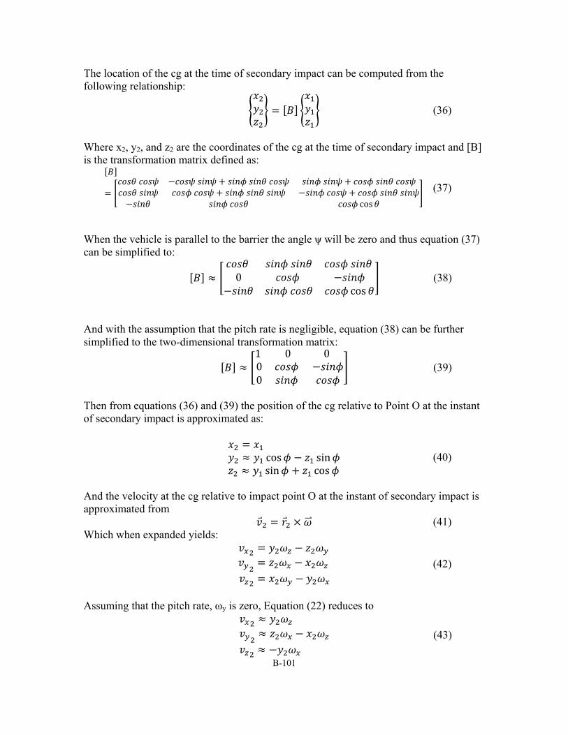
B-101

The location of the cg at the time of secondary impact can be computed from the following relationship:

(36)

Where x2, y2, and z2 are the coordinates of the cg at the time of secondary impact and [B] is the transformation matrix defined as:

cos (37)

When the vehicle is parallel to the barrier the angle ψ will be zero and thus equation (37) can be simplified to:

0cos

(38)

And with the assumption that the pitch rate is negligible, equation (38) can be further simplified to the two-dimensional transformation matrix: 1 0 0

00

(39)

Then from equations (36) and (39) the position of the cg relative to Point O at the instant of secondary impact is approximated as:

cos sinsin cos

(40)

And the velocity at the cg relative to impact point O at the instant of secondary impact is approximated from (41) Which when expanded yields:

(42)

Assuming that the pitch rate, ωy is zero, Equation (22) reduces to

(43)

B-102

The equations for approximating vehicle position and motion at the time of secondary impact with the barrier have not yet been verified with Equation (43). However, it is expected that these assumptions are valid as long as the impact angle remains “small” (e.g., around 15 degrees).

Phase 3 of Impact

The third phase of impact involves the side of the vehicle impacting against the face of the barrier, thus the impulse-momentum principles are again used to determine the kinematics of the vehicle resulting from the impulsive force. For simplicity, all frictional forces are ignored and it is assumed that the motion of the vehicle after impact is purely a rotation of the cg about the longitudinal axis of the barrier. It is also assumed that the vehicle remains in contact with the barrier and rotates about impact point O′. A freebody diagram is illustrated in Figure 33. Based on these assumptions the angular impulse about impact point O′ can be written as:

∗ (44) Where ∗ (45) Solving Equation (44) for yields

∗ (46)

B-103

Figure 33. Freebody diagram for Phase 3.

Phase 4 of Impact The final phase of the analysis is to determine if the vehicle has sufficient kinetic

energy to roll over the barrier based on its position with respect to the barrier and its angular velocity about the top of the barrier resulting from the secondary impact. The conservation of energy principle is defined as: (47) Where KEi and PEi are the initial kinetic and potential energies, respectively, of the vehicle immediately after impact against the barrier; likewise, KEf and PEf are the final kinetic and potential energies of the vehicle. The minimum criterion for rollover is when KEf is greater than zero. In other words, rollover occurs when there is sufficient kinetic energy to move the center of gravity of the vehicle directly over the top of the barrier.

B-104

Figure 34. Freebody diagram for analysis of truck rolling onto the barrier.

B-105

Rearranging Equation (47) and setting KEf equal zero yields the following condition for rollover:

1 (48)

The initial kinetic energy related to angular velocity is a function of the moment of inertia about Point O′ and the angular velocity about the roll axis and is defined by the following relationship: 1

2∗ (49)

The initial and final potential energy are defined as the weight of the vehicle times its height above the top of the barrier at the time of the secondary impact (i.e.,z2) and at its maximum height during the roll event (i.e., zmax), or ∗

and∗

(50)

As discussed earlier, after the secondary impact occurs, the vehicle will rotate about the longitudinal axis of the barrier. The final potential energy corresponds to the point where the arc of this rotation reaches its highest point directly over the top of the barrier. Noting that the radial arm of this rotation is equal to the distance from the center

of gravity of the vehicle to the top edge of the barrier, , then it follows that the critical maximum potential energy can be defined as:

∗ (51)

It is also of interest to compute the maximum roll angle during this phase of impact for cases when rollover does not occur. For example, in the following sections the results from the calculations developed here will be compared to the results from full-scale crash tests and finite element simulations. However, the vehicle did not roll over the barrier in any of these cases, except one (i.e., MASH test conducted on a 32-inch tall rigid barrier). In order to verify the analysis results the comparison will be based on the maximum roll angle as the vehicle is rolling over on top of the barrier.

The maximum vertical position of the cg during the roll event can be found from equations (48) and (50). For cases when rollover does not occur (i.e., the rollover ratio is less than one), the value for KEf will be zero when the vehicle reaches its highest point, i.e., when the kinetic energy is expended. Thus,

(52)

The maximum roll angle is equal to the angle of the cg relative to the top edge of the barrier when the cg is positioned at zmax minus the angle of the cg the relative to the top edge of the barrier when the cg is positioned at z1. Thus, the maximum roll angle can be computed from the following relationship:

(53)

B-106

Summary of Algorithm Input Variables

Impact Speed

Impact Angle

Vehicle Mass

Vehicle C.G. Coordinates (x1, y1, and zcg)

Barrier Height

Phase 1: Solve for Impulsive load and vehicle dynamics corresponding to initial impact Impulsive load (normal to barrier) sin

cos sin 1

Where ∗ 0.45 ∗ 3.05 ∗

3.85 ∗

Roll Rate (about vehicle fixed coordinate frame)

cos

Pitch Rate (about vehicle fixed coordinate frame)

sin

Yaw Rate (about vehicle fixed coordinate frame)

cos sin

Forward velocity (in vehicle fixed coordinate frame)

sin

Where Lateral velocity (in vehicle fixed coordinate frame)

cos

Phase 2: Calculation of vehicle position and motion immediately before secondary impact Total time until secondary impact

Roll Angle (vehicle fixed coordinate frame) C.G. Position

B-107

cos sinsin cos

C.G. Velocity

Phase 3: Solve for Impulsive load and vehicle dynamics corresponding to secondary impact Roll rate about impact point O

∗

Where ∗ Phase 4: Determine if Rollover/Vaulting is Likely and Compute Maximum Roll Angle Condition for Rollover/Vault

12

∗

1

Maximum Roll Angle

Application

The theoretical calculations developed in the preceding section are used here to compute the maximum roll angle of a single unit vehicles impacting against rigid, vertical-face, longitudinal barriers at a nominal speed and angle of 50 mph and 15 degrees, respectively. Several example cases are evaluated; these cases correspond to full-scale crash tests conducted by the Texas Transportation Institute. The input data for the calculations include:

Barrier height Vehicle weight Inertial properties (e.g., Ixx, Iyy, and Izz) CG height, zcg CG lateral coordinate relative to the vehicle fixed reference frame, y1 CG longitudinal coordinate relative to the vehicle fixed reference frame, x1 Impact velocity Impact angle

B-108

The “effective” position of the center of gravity of the vehicle is important to the accuracy of the results. For example, when the vehicle impacts the barrier, the front of the vehicle will crush inward altering the effective moment arm from the cg to the load point. Also, during the secondary impact, depending on the height of the truck-box relative to the top of the barrier, the truck bed may extend over the top of the barrier resulting in impact on the rear wheel axles against the barrier, thus the effective roll axis would be located at a line extending from the bottom of the box just above the rear wheels to the front of the vehicle; otherwise, the side of the truck-box would impact against the barrier and the roll axis would be a line from a point on the truck box to the front of the vehicle. Examples of these two scenarios are shown Figure 35, illustrating the difference in the location of the roll axis when the barrier is shorter than the bottom of the truck box and when the barrier is taller than the bottom of the truck box. Figure 35(a) was taken from TTI test RF476460-1 [Bullard10] and Figure 35(b) was taken from TTI test 420020-9b [Sheikh11].

Figure 35. Full-scale crash tests illustrating engagement points of vehicle during

redirection for (a) 32-inch tall barriesr [Bullard, 2010] and (b) 36-inch tall barriers. [Sheikh , 2011]

Based on these observations, calculations were made for three different analysis cases: Case 1: Y1 = Box width / 2 Case 2: Y1 = Track width / 2 Case 3: Y1 = Average of track width and box width

These dimensions were obtained from the “Vehicle Properties and Information” sheet in the test reports. The inertial properties of the test vehicles are typically not measured. Thus, the moment of inertia at the cg of the vehicle about the principle longitudinal axis is approximated based on the overall mass of the vehicle and its dimensional extents using the following relationship adopted from the revised BCAP equations in NCHRP 22-08 final report: [Mak94]

∗ 0.45 ∗ (54)

B-109

The moments of inertia about the remaining principle axes were approximated based on the ratio of inertial properties for a 45,500-lb single-unit truck defined in Labra et. al.[Labra76] where: 3.05 ∗

3.85 ∗ (55)

Table 25 shows the results for maximum roll angle of truck impact into various longitudinal barriers computed from the theoretical calculations. Also included in the table are the results from the corresponding full-scale crash test. In most of the 7069 series of tests, however, the location of the center of gravity was not documented in the summary report. Since all those tests were conducted with a test vehicle ballasted to 18,000 lb, the location of the cg was assumed to be the same as the cg location in Test 7069-15. In test 7069-15, the position of the cg relative to the point located directly below the center of the front bumper at the ground line was measured to be xcg = 152.8 in, ycg = 0 and zcg = 49.5 in.[Buth97]

Table 25. Comparison of maximum roll angle from theoretical calculations with

full-scale test results.

Figure 36 and Figure 37 show crash test photos from each of these tests from a downstream view point. Also included in the figures is a summary of the theoretical calculations and test results. As discussed earlier, it was assumed that analysis case 2

Shape

Height 

(in)

Weight

(lb)

Speed

(mph)

Angle

(deg)

IS

(kip‐ft)

zcg

(in)

x1

(in)

Case 

Type

y1

(in)

Rollover

Ratio

Model

(deg)

Test

(deg)

1 46.6 0.60 31

2 40.25 0.78 39

3 43.4 0.68 35

1 46.6 0.65 34

2 40.25 0.84 44

3 43.4 0.73 38

1 46.6 0.72 37

2 40.25 0.93 51

3 43.4 0.81 43

1 46.6 0.80 43

2 40.25 1.04 rollover

3 43.4 0.91 50

1 46.6 0.72 38

2 40.25 0.93 52

3 43.4 0.82 43

1 46.6 0.57 29

2 40.25 0.74 37

3 43.4 0.64 32

1 46.6 0.08 6

2 40.25 0.10 7

3 43.4 0.08 7

1 46.6 0.51 27

2 40.25 0.66 33

3 43.4 0.58 30

1 47.6 0.83 47

2 40.25 1.08 rollover

3 43.9 0.94 57

1 46.6 0.97 58

2 40.25 1.26 rollover

3 43.4 1.10 rollover

102.1

186.2

150.4 50.8 149.5

49.5

rollover

149.5 no rollover

152.8 18

44

152.8 31

25

152.8

152.8

RF 476460‐1b NJ‐Shape 32 22090 57.4 14.4

rollover 

on traffic 

side

40020‐9 Single Slope 36 22150 57.2 16.1 50.8 134.2 69

7118‐1 Safety shape 34 18000 51.7 14.6 49.5 153.6

7069‐34Vert. Wall 

w/ top rail42 18000 52.5 12.8 49.5

7069‐16 Vert. Wall 32 18000 50 14 88.0

81.3

7069‐15 Post‐and‐Beam 32 18000 50.8 15.1 49.5 152.8 24105.3

18050 52.1 14.8 49.5

93.9

106.8

114.3

7069‐9 F‐Shape 32 18050 47.3 15.3

7069‐12 NJ‐Shape 32 18000 51.6 15.5 49.5

49.5

7069‐11 F‐Shape 32

Test No.Barrier Impact Conditions Model Dimensions Maximum Roll Angle

7069‐8 F‐Shape 32 18050 46.7 15 49.5 152.8 3488.1

B-110

would serve as the most appropriate model for cases involving the 32-inch tall barriers; whereas, case 1 or 3 would be more appropriate for the taller barriers. Discussion of Results

From comparison with the full-scale crash tests, it seems that analysis case 2 tends to provide overly conservative results and that analysis case 1 generally provides results more comparable to full-scale tests. However, it is apparent in Figure 36 and Figure 37 that in many of the tests the vehicle had started redirecting away from the barrier while the vehicle was still rolled onto the top of the barrier. It is not clear if the vehicle had reached maximum roll angle before the vehicle started redirecting or if the redirection affected its maximum roll angle. This event, of course, was not included in the development of the theoretical model. In fact, there are many variables involved in these crash events that are ignored for the sake of simplicity.

The basic test parameters are very similar for most of the tests (i.e., most are consistent with test Report 350 test procedures). In particular, the impact speed and angle were nominally 50 mph and 15 degrees; the vehicle weight was nominally 18,000 lb; the vehicles were all of similar type; the barrier height was 32 inches in most cases. Thus, the results from the model were very similar in most cases, as would be expected. The primary difference in these tests was the shape of the barrier face. Cases involving vertical face barriers (i.e., 7069-15, 7069-16, 7069-34) generally resulted in lower roll angles than the other barrier types; followed next by the F-shape barrier and then by the NJ-shape and the constant-slope barrier types.

Regarding the vertical face barriers, the model significantly over-predicted the maximum roll angle by 25-30% based on comparison of analysis case 1 with the full-scale test results. For the F-shape, the model for analysis case 1 tends to provide reasonable results; and for the NJ-shape and the constant slope barrier types, the model for analysis case 2 tends to provide the more reasonable results.

The rollover-barrier-algorithm in RSAPv3 is based on case 1, where y1 is defined as the half-width of the vehicle.

B-111

Figure 36. Crash test photos and summary of maximum roll angles.

B-112

Figure 37. Crash test photos and summary of maximum roll angles (continued).

B-113

REDIRECTION Redirection is only considered for impacts with longitudinal hazards. Recall that

impact with longitudinal hazards can result in one of six possible post-impact scenarios: (1) stop in contact with hazard, (2) structural penetration, (3) rollover top of hazard, (4) vault over hazard, (5) redirection and (6) redirection with rollover.

The probability of redirection (without rollover) from a longitudinal hazard is determined in RSAPv3 based on the probability that structural penetration and rolling over the hazard did not occur. Redirection is generally the desired outcome for line hazards; in fact, longitudinal barriers are designed specifically to accomplish redirection. However, even when a vehicle is successfully redirected there is still a possibility of rolling over or striking another hazard after redirection. In order to account for these secondary crash events, it was necessary to determine the factors that influence their occurrence. For example, when a vehicle is redirected from a hazard, the likelihood of a subsequent impact depends upon the vehicle’s path and the distance that it travels. The redirection path is influenced by many factors including, impact angle, impact speed, vehicle type, barrier type (i.e., rigid, semi-rigid, flexible, etc.), vehicle damage (e.g., wheel assembly damage), vehicle-to-barrier interaction (e.g., snagging), and driver reaction, to name a few. In the context of an RSAP analysis, however, only a few of these factors are relevant.

The following sections discuss the influence of three factors on redirection path (i.e., impact angle, barrier type and vehicle type) and the methodology RSAP uses to analyze the possibility of secondary collisions resulting from redirection, including rollover after redirection.

Factors Influencing Redirection Path

17-22 Database Review The 17-22 crash reconstruction database was reviewed in order to identify cases

involving impacts with longitudinal barriers. This subset of cases was further refined to include only those cases where the longitudinal barrier was the first object struck and the impact did not result in penetration. Additional cases were then excluded if there were insufficient data for determining the post redirection path (e.g., final longitudinal coordinate of the vehicle was the same as the initial redirection coordinate). It was assumed that many of those cases involved end-on impacts with guardrail terminals and the vehicle was brought to a stop without exiting from the system or possibly that the redirection path was simply not recorded.

Of the 892 crash cases in the 17-22 database only 33 cases satisfied these criteria. These included 12 cases involving rigid barriers (i.e., concrete safety shapes and bridge rails); 17 cases involving semi-rigid barriers (i.e., strong-post guardrail); and four cases involving flexible barriers (i.e., cable and weak-post guardrail).

The departure and subsequent redirection trajectory paths for each of these crash cases were plotted. The redirections rarely resulted in a straight-line path from the barrier. For example, the redirection would start in one direction and then turn in another depending on a myriad of unrecorded factors. In many cases, particularly collisions with flexible barriers and semi-rigid barriers, it was not possible to determine the exact point when the vehicle exited the barrier. Impacts with such barriers generally result in the

B-114

vehicle remaining in contact with the barrier over greater distances. Further, as a result of barrier deflection, the redirection paths appear to penetrate behind the barrier, as illustrated in Figure 38 which shows a redirection path from the 17-22 database involving a semi-rigid barrier.

The redirection angle with respect to the longitudinal direction of the barrier was computed based on the “apparent” redirection path determined from visual inspection of the trajectory plot, as illustrated in Figure 38. Figure 39 and Figure 40 show plots of the approximate redirection angle versus impact angle for rigid barriers and for semi-rigid and flexible barriers, respectively. These plots seem to indicate that redirection angles are not strongly correlated to the angle of impact, except that the redirection angle is relatively low or zero for impact angles greater than 20 degrees involving impact with rigid barriers.

Figure 38. Departure and redirection path from a crash case in the 17-22 crash reconstruction database.

Impact PointSemi‐Rigid Barrier

Barrier Deflection

Approximate Linear Redirection Path

Actual Redirection Path

‐30

‐25

‐20

‐15

‐10

‐5

0

5

Lateral O

ffset from Edge‐Line

Longitudinal Distance Along Roadway (m)

B-115

Figure 39. Plot of redirection angle vs. impact angle for collisions with rigid

barriers.

Figure 40. Plot of redirection angle vs. impact angle for collisions with semi-rigid

and flexible barriers.

Figure 41 and Figure 42 show plots of the cumulative distribution of redirection angles for rigid barriers and for semi-rigid and flexible barriers, respectively. There were not enough data to make confident conclusions, but from the handful of available cases the mean redirection angle for impacts with rigid barriers was 8.8 degrees and the 50th percentile redirection angle was zero degrees. The 15th and 85th percentile redirection angles for impacts with rigid barriers were approximately zero and 14 degrees, respectively. Likewise, the mean redirection angle for the non-rigid barriers was 20.8 degrees and the 50th percentile was approximately 16 degrees. The 15th and 85th

0

10

20

30

40

50

60

70

0 10 20 30

Redirection Angle (deg)

Impact Angle (deg)

Semi‐Rigid and Flexible Barrier

Semi‐Rigid Barrier

Flexible Barrier

B-116

percentile redirection angles for impacts with non-rigid barriers were 4 degrees and 31 degrees, respectively.

Figure 41. Cumulative distribution of redirection angles for rigid barriers from 17-

11 crash reconstruction database (passenger vehicles only).

Figure 42. Cumulative distribution of redirection angles for semi-rigid and flexible

barriers from 17-11 crash reconstruction database (passenger vehicles only).

Full-Scale Crash Tests Review A series of crash tests on ten bridge rails and two transition systems was

conducted by the Texas Transportation Institute (TTI) from 1987 to 1993.[Buth97] The test series included a total of 37 tests involving five vehicle types: small car, pickup, single unit truck, intercity bus and tractor-semitrailer. Those tests were conducted according to the then-current crash test requirements for assessing safety performance of

0

0.1

0.2

0.3

0.4

0.5

0.6

0.7

0.8

0.9

1

0 10 20 30 40 50 60

CDF  (Percent Less)

Redirection Angle (deg)

Rigid Barrier

0

0.1

0.2

0.3

0.4

0.5

0.6

0.7

0.8

0.9

1

0 10 20 30 40 50 60 70

CDF  (Percent Less)

Redirection Angle (deg)

Semi‐Rigid  and Flexible Barrier

B-117

longitudinal barriers.[Buth97] In general, the tests involving passenger vehicles were conducted at nominal impact speeds of 50 and 62 mph and a nominal impact angle of 20 degrees; while tests involving commercial vehicles were conducted with a nominal impact speed of 50 mph and a nominal impact angle equal 15 degrees.

Redirection Angle

The results from these tests were reviewed to determine the influence of vehicle type on redirection angle. Table 26 shows a summary of the impact conditions and resulting exit conditions for each of 37 full-scale tests. Figure 43 and Figure 44 show the cumulative distribution for redirection (exit) angles resulting from passenger vehicle impacts and from commercial vehicle (e.g., trucks and buses) impacts, respectively. Regarding passenger vehicles, the mean redirection angle was 7.4 degrees with a 50th percentile value of 6.5 degrees. Eighty percent of passenger-vehicle impacts resulted in redirection angles between 5 and 9 degrees.

Regarding commercial vehicles, the mean redirection angle was 2.4 degrees with a 50th percentile value of zero degrees. With the exception of one case, all truck tests resulted in redirection angles of 5 degrees or less.

B-118

Table 26. Summary of impact and exit conditions from test series 7069.[Buth97]

Speed (mph)

Angle (deg)

Kinetic Energy (ft-lb)

Speed (mph)

Angle (deg)

Kinetic Energy(ft-lb)

ExitKinetic E.

KE(1 - sinθ) Error

ExitSpeed(mph) Error

1,961 58.7 20 225,700 48.5 5.2 154,077 148,506 -3.6% 47.6151 -1.8%1,965 60.5 21 240,243 48.6 6.2 155,029 154,147 -0.6% 48.4617 -0.3%1,965 61.7 18.7 249,868 50.3 1 166,064 169,757 2.2% 50.8562 1.1%1,966 60.1 21.4 237,197 53 6.2 184,464 150,649 -18.3% 47.8965 -9.6%1,967 51.7 20.8 175,615 40.8 6.1 109,371 113,253 3.5% 41.5178 1.8%1,970 52.2 19.7 179,302 42.7 7.1 119,977 118,860 -0.9% 42.5007 -0.5%1,970 51.2 20.5 172,498 43 6.8 121,669 112,088 -7.9% 41.2722 -4.0%1,970 60.3 19.8 239,264 50.6 6.6 168,478 158,216 -6.1% 49.0348 -3.1%1,970 59.9 20.1 236,100 50.8 6.4 169,813 154,962 -8.7% 48.5279 -4.5%1,970 51.6 19.9 175,203 44.3 9.1 129,137 115,568 -10.5% 41.9080 -5.4%1,970 60.5 19.9 240,854 47.7 6.9 149,720 158,872 6.1% 49.1363 3.0%5,565 45.3 20.2 381,451 37.2 5.3 257,234 249,737 -2.9% 36.6539 -1.5%5,565 60.4 20.4 678,135 55.6 9 574,635 441,756 -23.1% 48.7495 -12.3%5,565 47.7 19 422,940 42.8 8.9 340,510 285,244 -16.2% 39.1731 -8.5%5,565 61.4 18.3 700,775 50 8.2 464,710 480,737 3.4% 50.8549 1.7%5,566 45.6 18.8 386,589 38 6.2 268,465 262,005 -2.4% 37.5400 -1.2%5,568 62.6 19.4 728,828 53.5 5.4 532,333 486,739 -8.6% 51.1576 -4.4%5,570 55.3 19.6 568,961 44.8 6.5 373,412 378,102 1.3% 45.0805 0.6%5,570 62.7 19 731,421 41.9 9 326,633 493,293 51.0% 51.4916 22.9%5,724 57.7 20.6 636,544 35.8 20.6 245,043 412,581 68.4% 46.4533 29.8%5,737 46.1 20.9 407,252 35.9 10.9 246,974 261,970 6.1% 36.9739 3.0%5,759 59.7 20.2 685,603 47 6.4 424,932 448,866 5.6% 48.3054 2.8%5,780 65.4 20.4 825,772 56.9 7.4 625,071 537,931 -13.9% 52.7851 -7.2%5,797 63.6 19.2 783,239 57.6 5.8 642,429 525,658 -18.2% 52.1029 -9.5%

18,000 50.8 15.1 1,551,590 N/A 0 N/A 1,147,394 43.6849 18,000 50 14 1,503,106 34.2 5 703,237 1,139,471 62.0% 43.5338 27.3%18,000 51.6 15.5 1,600,844 N/A 2 N/A 1,173,037 44.1704 18,000 52.1 14.8 1,632,018 N/A 0 N/A 1,215,126 44.9558 18,000 51 13.7 1,563,831 N/A 0 N/A 1,193,456 44.5532 18,000 53.5 12.8 1,720,906 44.6 3.5 1,195,967 1,339,642 12.0% 47.2030 5.8%18,000 51.4 14.7 1,588,458 N/A N/A N/A 1,185,374 44.4020 18,000 51.6 14.6 1,600,844 N/A 11 N/A 1,197,320 44.6252 18,050 46.7 15 1,314,886 N/A 5 N/A 974,568 40.2049 18,050 47.3 15.3 1,348,890 34.5 2 717,616 992,954 38.4% 40.5824 17.6%40,560 55.7 15.7 4,203,251 42.5 0 2,447,106 3,065,849 25.3% 47.5705 11.9%50,000 52.2 14 4,550,802 N/A 0 N/A 3,449,864 45.4493 50,050 51.4 16.2 4,416,796 N/A 0 N/A 3,184,549 43.6449

Weight(lbs)

EstimatedImpact Conditions Exit Conditions

B-119

Figure 43. Cumulative distribution of redirection angles for passenger vehicles from

full-scale crash test series 7069.

Figure 44. Cumulative distribution of redirection angles for commercial vehicles

from full-scale crash test series 7069.

RSAPv3 Implementation

Redirection without Rollover Ideally, all of the possible redirection paths should be analyzed for subsequent

impacts; the crash costs then computed based on the average cost of all the possible redirection scenarios. However, the number of reconstructed redirection paths currently available is very small (i.e., total of 33), and it is not possible to obtain a representative sample consisting of all possible redirection paths for any given impact scenario. Further,

0

0.1

0.2

0.3

0.4

0.5

0.6

0.7

0.8

0.9

1

0 5 10 15 20

CDF (Percent Less Than

)

Exit Angle (deg)

Passenger Vehicles

0

0.1

0.2

0.3

0.4

0.5

0.6

0.7

0.8

0.9

1

0 5 10 15 20

CDF (Percent Less Than

)

Exit Angle (deg)

Trucks and Buses

B-120

such an analysis would require extensive computational time and resources, as every departure trajectory that strikes a longitudinal barrier would spawn many more trajectory paths which would, in turn, be analyzed for subsequent collisions. Each of those redirection trajectories that resulted in secondary collisions would again spawn more trajectory paths, and this process would continue until the vehicle was brought to rest for all spawned trajectories through deceleration and energy expenditure.

RSAPv3 is programmed to perform this type of analysis; however, for the sake of computational efficiency a maximum of two redirection paths are examined in RSAPv3. Further, the redirection paths are assumed to be linear. The exit conditions for these redirection trajectories are dependent on the vehicle type, barrier type and impact angle. For the case of passenger vehicles impacting rigid barriers, the most probable redirection angle is less than 9 degrees, based on the cumulative distribution plots of Figure 41 and Figure 43. Figure 43 also indicates that redirection angles ranging 5 to 9 degrees are equally probable; note that these two values also correspond to the 15th and 85th percentile values, respectively. Thus, for the case of passenger vehicles impacting rigid longitudinal barriers, RSAPv3 evaluates two redirection paths with exit angles of 5 and 10 degrees, measured with respect to the barrier. Each of these redirection paths are considered to be equally probable regarding calculations of subsequent crash costs.

For the case of passenger vehicles impacting semi-rigid and flexible longitudinal barriers, the cumulative distribution plot of Figure 42 indicates that redirection angles ranging from 0 to 30 degrees are equally probable, with the 50th percentile found to be 16 degrees. In these cases, RSAPv3 evaluates two redirection paths corresponding to exit angles of 10 and 20 degrees, measured with respect to the barrier; and each of these redirection paths are considered to be equally probable regarding calculations of subsequent crash costs.

For the case of trucks impacting all barrier types, the cumulative distribution plot of Figure 44 indicates that the most probable redirection angle is zero degrees and that in 90 percent of these full-scale test cases the redirection angle is less than 5 degrees. These values were determined from full-scale crash tests with impact conditions of 15 degrees and 50 mph and may not be relevant at other speeds and angles; however, until more data (e.g., field data or test data) is available, the redirection paths for trucks will be evaluated in RSAPv3 with exit angles of 1 and 5 degrees, measured with respect to the barrier. Each of these redirection paths are considered to be equally probable regarding calculations of subsequent crash costs.

Redirection is not considered for motorcycles in RSAPv3, because it is assumed that motorcycle collisions generally result in passenger ejection and then falling onto its side and skidding to a stop while still in contact with the barrier.

Speed Change Due to Redirection When vehicles impact against longitudinal barriers, some of the kinetic energy is

expended through plastic deformation of the vehicle, friction between vehicle and barrier, friction between tires and ground, friction between internal components of the vehicle, and elastic deformations that get trapped as vibrational energy. The result is a reduced velocity of the vehicle as it redirects from the barrier system.

B-121

It is not possible to accurately calculate the exact reduction in kinetic energy of the vehicle without conducting a detailed analysis of the crash event (e.g., finite element analysis or full-scale crash test). It seems logical, however, to assume that the amount of kinetic energy loss is related to the angle of impact. In other words, a vehicle impacting at a high angle would be expected to redirect and exit the system at a much lower velocity than it would when impacting at a low impact angle. The following relationship was used to approximate the redirection energy and speed as a function of initial impact energy and the sine of the impact angle: 1 sin

2

(56)

In Equation (56) is the initial impact energy, θ is the impact angle, m is the mass of the vehicle, is the estimated kinetic energy of the vehicle upon exiting the barrier, and is the resulting estimated exit velocity of the vehicle. This is an approximation developed based on engineering judgment, but it was found to be reasonably accurate for estimating the exit speeds for passenger vehicles in the full-scale tests shown in Table 26. In eighty percent of those test cases, the estimated exit speed was within 10 percent of the measured value.

Rollover after Redirection As mentioned previously, redirection is generally the desired outcome for impacts

with line hazards (e.g., guardrail and median barrier), but they sometimes result in secondary collisions including rollover. As with all accidents, there are many factors that influence their occurrence and outcome, which cannot be accounted for in these simple calculations. Rolling over after redirection, for example, is usually associated with vehicle instability which may result from the dynamics of the initial impact event (e.g., high roll, pitch or yaw exit angles), poor steer/braking reaction of the driver during redirection, or vehicle tripping due to soft soil and/or damage to the vehicle’s suspension.

RSAPv3 determines the probability of rollover after redirection differently for different vehicle types. For passenger vehicles, rollover after redirection is determined solely from crash statistics, which are generally considered more reliable for predicting collision outcomes since they inherently account for all influences leading to the collision event. The statistics data for redirection rollovers is provided on the RSAPv3 “Severity” worksheet for each hazard type and can be readily updated as warranted. If no value is provided, a default value of zero is assumed. As was the case for hazard penetrations, meaningful statistics data for rolling over after redirection are generally only available for the passenger-class of vehicles, as the crash data is dominated by passenger vehicles. Therefore, for trucks, the probability of rolling over after redirection must be determined based on the mechanics of the collision event. The algorithm implemented in RSAPv3 was adopted from the rollover algorithm developed by Mak and Sicking in NCHRP Project 22-8.[Mak94] The algorithm, which is shown in Equation (57), was developed based on simplified impulse and momentum principles, where “the vehicle was predicted to rollover on the traffic side of the hazard if

B-122

the vehicle’s roll inertia after impact with the barrier was sufficient to raise the center of gravity (of the vehicle) above the point of neutral equilibrium.”[Mak94]

.

(57)

Where: Vrr = Minimum velocity in ft/sec at which the vehicle will rollover on the traffic side of the hazard,

B = The width of the vehicle in feet g = The acceleration due to gravity (i.e., 32.2 ft/s2),

Hcg = The height of the vehicle center of gravity in inches, Hb = The height of the barrier in inches and

Θ = The impact angle in degrees. This formulation assumes that the barrier forces act at the top of the barrier. The

formulation further assumes that roll angles do not develop when the center of gravity of the vehicle is lower than the top of the barrier; thus, RSAPv3 does not consider trucks rolling over in those cases.

It was determined in the NCHRP 22-8 study that Equation (57) was capable of predicting rollover with reasonable accuracy, based largely on the fact that the benefit-cost predictions from BCAP showed very little sensitivity to the rollover predictions.

There may be some concern, however, regarding the severity of rollover accidents for trucks. It is expected that occupant injury in truck rollovers would be, in general, less severe than injuries resulting from passenger vehicle rollovers. Trucks tend to only roll a quarter-turn onto their side, whereas passenger vehicles can roll multiple quarter-turns and sometimes result in passenger ejection which is more hazardous than when the occupant is retained in the vehicle. A similar conclusion was found by Stein and Jones in their analysis of heavy truck accidents on interstate highways in the 1980s. Their research showed that of all truck rollover accidents studied only 49 percent resulted in occupant injuries.

Regarding overall crash cost, however, one must take into consideration that passenger vehicles are (1) generally not as expensive as trucks and (2) often tend to have multiple occupants; whereas trucks generally have only a single occupant. With that said, RSAPv3 currently does not discriminate regarding crash cost calculations for rollover events. That is to say, the severity of a rollover is considered the same for all rollovers, regardless of the cause of the rollover or vehicle type. Any differences in crash cost (i.e., EFCCR) for rollovers arise only from differences in speed of the vehicle at the time of rollover.

COMPUTING TRAJECTORY EFCCR The RSAPv3 severity model is based on the equivalent fatal crash cost ratio

(EFCCR) that will be discussed in the next section. This section describes how multiple crash events on one trajectory are combined to determine the severity of each encroachment trajectory. The average EFCCR of a collision is computed according to

B-123

the hazard severity (i.e., EFCCR) of each hazard, the impact speed and the probability of the collision event occurring. Instead of assigning a higher “blanket” severity to a hazard to account for secondary collisions, such as penetrating a median barrier and crossing the median into opposing traffic lanes, RSAPv3 will continue to evaluate the trajectory for subsequent collisions after impact with the barrier until the velocity of the vehicle goes to zero. So for a given trajectory, the total EFCCR is the collective sum of all collisions resulting from that trajectory case (e.g., initial impact and secondary impacts due to penetration, redirection and rollover).

Example: Computing EFCCR for an encroachment path The encroachment scenario in Figure 45 will be used to illustrate the procedure

for computing the total crash cost (EFCCR) of an encroachment. The EFCCR associated with each possible collision event for the encroachment case is computed and shown in Table 27; the effective EFCCR value for each collision is then determined by multiplying the EFCCR value for each collision by the probability of the collision event occurring (POC). Figure 46 illustrates the flow chart for the collision probability calculations.

B-124

Figure 45. Example illustrating collision prediction process in RSAPv3 for a single

encroachment

Table 27. Example of computing EFCCR for an encroachment path

The following is a summary of the collision prediction process using the example

in Figure 45 and Table 27. The road segment in this example is a divided roadway with a median barrier separating the opposing lanes of traffic (note that only the primary traffic lanes are shown in the figure). A water hazard is located on the right-side of the roadway and is protected by a strong-post w-beam guardrail. The median barrier is located four feet from the left edge line, the guardrail is located four feet from the right edge line, and the water hazard is located 100 feet downstream of the encroachment point.

The vehicle encroaches onto the right roadside at Point A at a velocity of 58.8 ft/s. The trajectory path results in an impact with the guardrail at Point B at an impact speed of 55.01 ft/s. Before evaluating the impact with the guardrail, RSAPv3 first considers the

A

Guardrail

Median Barrier

Water Hazard

CD

E

B

A Encroachment ‐ 58.8 ‐ ‐ ‐

A‐B Rollover 0.0220 56.85 4.67E‐03 0.0046 2.16E‐05

B Impact with Guardrail 0.0178 55.01 3.42E‐03 0.9954 3.40E‐03

B‐C Rollover after redirection 0.0220 49.3 3.04E‐03 0.0050 1.52E‐05

C No impact with median barrier 0.0012 ‐ ‐ 0.4728 ‐

B‐D Rollover after redirection 0.0220 49.3 3.04E‐03 0.0050 1.52E‐05

D Impact with median barrier 0.0012 17.51 7.44E‐06 0.4728 3.52E‐06

B‐E Rollover after penetration 0.0220 35.77 1.16E‐03 0.0008 9.30E‐07

E Impact with water hazard 0.0782 18.448 5.67E‐04 0.0390 2.21E‐05

EFCCR65EVENT Effective 

EFCCR

impact 

velocity 

(ft/s)

EFCCR POC

B-125

probability of the vehicle rolling over prior to the impact event (i.e., rollover between Point A and Point B). In this example, the probability of rolling over prior to impact was determined to be 0.0046 and the representative speed of the rollover was determined to be 56.85 ft/s. Based on the impact velocity, the probability of the rollover, and given that the EFCCR65 for rollover is 0.022 from the RSAPv3 “severity” worksheet, the effective EFCCR of the rollover event was computed to be 2.16E-5.

RSAPv3 then evaluates the impact with the guardrail. Since there was a 0.0046 probability of rollover before impact, the resulting probability of impact with the guardrail at Point B was thus 0.9954. Then, based on the impact velocity, the probability of the collision, and given that the EFCCR65 for the guardrail is 0.0178, the effective EFCCR for the collision with the guardrail was computed to be 3.40E-3. Recall that when RSAPv3 detects impact with a line hazard, it evaluates the probability of both redirection and penetration. Based on the impact conditions in this example, the probability of redirection and penetration was determined to be 0.9556 and 0.0398, respectively.

Regarding redirection, RSAPv3 evaluates two possible redirection paths and each path is given equal probability of occurrence. There is a probability of rollover for each redirection path which was calculated to be 0.005 (i.e., from Point B to C and from Point B to D). The corresponding EFCCR value was computed to be 1.52E-5 in each case. The redirection path from B to C ended with zero velocity (due to deceleration) with no further collisions. The redirection path from Point B to Point D resulted in a secondary impact with the median barrier at a speed of 17.51 ft/s. The effective crash cost for this event was calculated from the impact speed, the severity rating for the median barrier (i.e., EFCCR65=0.0012) and the probability of the redirection path occurring (i.e., POC = 0.4728). The resulting effective EFCCR for the collision event at Point D was calculated to be 3.52E-6.

RSAPv3 then evaluates the penetration trajectory path for collisions, which in this case results in a collision with the water hazard at Point E at an impact speed of 18.45 ft/s. Before evaluating the impact with the water hazard, RSAPv3 first considers the probability of the vehicle rolling over prior to the impact event (i.e., rollover between Points B and E). The probability of rollover after penetration was 0.0008; the effective EFCCR for the rollover event was computed to be 8.99E-7, based on the severity rating for a rollover, the speed of the rollover, and its probability of occurrence. RSAPv3 then evaluates the impact with the water hazard. The probability of impact with the water hazard is computed as the probability that penetration occurred (i.e., 0.0398) minus the probability that rollover occurred before the collision with the water hazard (i.e., 0.0008), which results in a probability of 0.039. Then based on the impact velocity, the probability of the collision and given that the EFCCR65 for the water hazard is 0.0782, the effective EFCCR for the collision was computed to be 2.21E-5. The total crash cost for this example trajectory is then computed as the collective sum of each possible collision event and its probability of occurrence (i.e., effective EFCCR in Table 27), which results in a total crash cost ratio of 0.003481 or $20,886 in 2009 dollars.

B-126

Figure 46: Flow chart of possible collisions resulting from the example trajectory in

Figure 45 and their probability of occurrence.

B-127

SEVERITY PREDICTION MODULE Once the probability of leaving the roadway (i.e., Encroachment Probability

Module) and the probability of striking an object (i.e., Crash Prediction Module) have been calculated, it is necessary to estimate the likely average severity of the crash in order to appropriately apportion the crash costs. A Severity Index (SI) unique to each roadside hazard has been used past roadside design benefit-cost programs to represent the severity of striking a roadside as described in NCHRP Report 492.[Mak03] Previous research studies have proposed replacing the SI method with methods which use the observed severity distribution of police-level reported crashes.[Mak98] Those prior attempts to include police-level reported crashes in determining crash severity have been extended and implemented in RSAPv3. The following chapter provides a review of the traditional SI approach compared to collected crash data and presents the new approach for estimating crash severity which has been implemented into RSAPv3.

BACKGROUND The Severity Index (SI) used in prior versions of RSAP is a linear function of

speed. For example, the slope of the SI-speed curve for a crash with an eight inch tree or wooden utility pole is 0.0839 SI/mph. RSAP 2.0.3 would randomly generate an impact speed which was multiplied by the slope of the SI-speed curve and mapped to the generic distribution of crash severities shown in Table 28. When the resulting SI equaled 0.5, 100 percent of the crashes were categorized as “Property Damage Only” crashes whereas when the SI equaled 10, 100% of crashes were assumed to be fatal. The slope values for the SI curves were based primarily on engineering judgment. The crash cost associated with each SI severity distribution is also shown in Table 28 based on the 1994 FHWA recommended crash costs.[FHWA94] In the far right column, the average crash cost for each SI severity distribution is divided by the cost of a fatal crash to yield an equivalent fatal crash cost ratio (EFCCR). The EFCCR is simply a dimensionless measure of crash cost that can be scaled to any particular year assuming that the underlying distributions of severity remain constant.

B-128

Table 28. NCHRP 492 Generic Severity Distributions.

1994 FHWA Recommended Crash Costs Avg. Crash Cost

EFCCR$0 $2,000 $19,000 $36,000 $180,000 $2,600,000

SI None O C B A K 0 100.0% $0 0.0000

0.5 100.0% $2,000 0.0008

1 90.4% 7.3% 2.3% $4,023 0.0016

2 71.0% 22.0% 7.0% $8,120 0.0031

3 43.0% 34.0% 21.0% 1.0% 1.0% $42,680 0.0164

4 30.0% 30.0% 32.0% 5.0% 3.0% $104,820 0.0403

5 15.0% 22.0% 45.0% 10.0% 8.0% $246,680 0.0949

6 7.0% 16.0% 39.0% 20.0% 18.0% $521,220 0.2005

7 2.0% 10.0% 28.0% 30.0% 30.0% $846,020 0.3254

8 4.0% 19.0% 27.0% 50.0% $1,356,200 0.5216

9 7.0% 18.0% 75.0% $1,984,920 0.7634

10 100.0% $2,600,000 1.0000

The SI approach to determining crash severity has been widely used but never validated or compared to real-world crash data. One of the only databases with reconstructed speeds is the Longitudinal Barrier Special Studies (LBSS) database. Hunter, Stewart and Council used the LBSS data to investigate differences between impacts with different longitudinal barriers using a logit regression model to estimate the probability of observing a fatal crash.[Hunter93] The SI approach assumes that every longitudinal barrier has the same severity distribution (i.e., 0.1944 SI/MPH). Their model included the barrier type, vehicle weight, as well a reconstructed impact speed and angle. While their purpose was not explicitly to validate the SI approach, they did find that there were differences between barrier types. In fact, barrier type was the most significant predictor variable whereas the impact conditions (i.e., speed and angle) were relatively weak predictors of severity. While crash severity should be a function of the full range of impact conditions, there are many variables that must be accounted for and most of these variables are either not measured or are immeasurable so there has never yet been a strong relationship developed between impact speed, angle and orientation and crash severity as measured by the level of occupant injury.

Speed and Crash Severity Police reported crashes generally use the KABCO crash severity scale to

document vehicle occupant injury severity where a “K” is a fatal crash proceeding in decreasing severity to an “O” which is a property damage only crash. The SI method uses values between zero and 10 and then translates the index into an assumed KABCO distribution (i.e., Table 28) which is then weighted by crash costs to determine the average crash cost at a given impact speed. Throughout the remainder of this chapter, the

B-129

crash severity data and the SI data have been mapped to the 2009 comprehensive crash costs to allow for direct comparisons. The Benefit/Cost Module chapter of this Manual discusses crash costs.

The case of crashes involving utility poles will be examined to illustrate the use of the SI method. Utility poles are a useful category of objects to study since (1) they are fairly uniform in size, (2) they are generally dangerous fixed roadside objects and (3) they are ubiquitous on the roadway network except on high-speed divided highways. Several SI values are recommended for utility poles in NCHRP Report 492 ranging from 0.0819 for 8 inch poles up to 0.1017 for poles greater than 12 inches in diameter. The estimated average crash costs as a function of impact speed using the SI method is shown in Figure 47. The SI value (i.e., 0.0819 SI/MPH) used in this comparison was based on an 8-inch diameter utility pole which is thought to be a relatively common size.

The severity of utility pole crashes can be obtained from a variety of sources but two particularly useful sources are the FHWA Highway Safety Information System data for Washington State (WSDOT HSIS) and the Maine Department of Transportation (MEDOT) crash databases. Both sets of data are based on police-level crash reports and both include the severity of the crash in the usual KABCO scale as well as the posted speed limit of the roadway. Using the severity distributions at each posted speed in the WSDOT HSIS and MEDOT databases, the average expected crash cost in 2009 dollars can be plotted versus the posted speed as shown in Figure 47.

Also shown in Figure 47, the traditional formulation of the SI does not do a very good job of predicting crash costs for utility pole crashes. There are, however, some important differences between the SI-method predictions and the observed crash data that should be pointed out. First, the SI-method predictions are based on impact velocity whereas the observed crash data is based on posted speed. The relationship between posted and impact speed can be examined with the NCHRP 17-22 database which is a set 890 cases that have been reconstructed based on scene and vehicle evidence.[Mak10] The average impact speed in the NCHRP 17-22 is always less than the posted speed limit so posted speed is an over estimate of average impact speed. Second, the observed data, by definition, is missing unreported collisions which are typically low severity crashes. These two differences, however, would suggest that the observed crash data should over estimate crash severity since low severity crashes are excluded and impact speed is, on average, over estimated. Figure 47 throws into question the subjective values assumed in the SI relationships and the basic assumption that SI and speed can be mapped linearly.

B-130

Figure 47. SI-Method Predicted Crash Costs versus Observed Crash Costs of

Utility Pole Crashes in Washington State and Maine.

Sicking in NCHRP Report 638 found much the same when investigating guardrail

crashes in Kansas.[Sicking09] He compared the results of analysis conducted with RSAP 2.0.3 with the results of an examination of the Kansas guardrail, median barrier and bridge rail data and found that the average crash costs from RSAP 2.0.3 were a little over twice as large as the Kansas longitudinal barrier crash data indicating that RSAP 2.0.3 was over predicting the severity and, hence, the crash costs.[Sicking09] Recall RSAP 2.0.3 uses SI to perdict crash costs. Sicking resolved this by adjusting the RSAP severity indices downward until the average crash costs from RSAP 2.0.3 agreed with the Kansas data. One of the important reasons for this over-prediction identified by Sicking is that RSAP 2.0.3 and the traditional severity model ignores unreported crashes which are generally low-cost property damage only crashes. Improving the accuracy of crash costs in RSAPv3 requires a different approach to modeling crash severity that is more closely tied to observable crash data and that also accounts for unreported crashes.

The relationship between speed and crash severity in general has been well established by many researchers.[Nilsson81;Bowie94;Joksch93;ODay82] As stated in an FHWA synthesis on speed affects and crash severity:

“The relationship between vehicle speed and crash severity is unequivocal and based on the laws of physics. The kinetic energy of a moving vehicle is a function of its mass and velocity squared. …. Generally, the more kinetic energy to be dissipated in a collision the greater the potential for injury to vehicle occupants. Because kinetic energy is determined by the square of the vehicle’s speed rather than by speed alone, the probability of injury and the severity of injuries that occur in a crash, increase exponentially with vehicle speed.” [FHWA88]

$-

$500,000

$1,000,000

$1,500,000

$2,000,000

$2,500,000

0 20 40 60 80 100 120

2009

Cra

sh C

osts

Posted Speed Limt (MPH)

SI Prediction for 8-inch Utility Pole

2002-2006 WSDOT HSIS Utility Pole Crashes

1994-1998 MEDOT Utility Pole Crashes

B-131

The linkage, therefore, between speed and severity has been made both statistically and based on the physics of vehicle crashes. Nilsson showed that for all types of crashes the number of injury crashes increases as a square of the ratio of velocities; to the third power for severe injury crashes and to the fourth power for fatal crashes.[Nilson81] Similar results have been obtained in the US by Bowie, Joksch and O’Day to name several.[Bowie94;Joksch93;ODay82] Nilsson showed that the ratio of injury crashes prior to a change in average travel speed to those after is proportional to the ratio of speed squared:

Where PI1 and PI2 are the number of injury crashes before and after a change in

average speed and V1 and V2 are the speeds before and after. For example, Nilsson’s expression would indicate that a particular rural two lane road that experiences 10 injury

crashes/mi/yr when the average travel speed is 55 mi/hr would experience on average 6.7 injury crashes/mi/yr if the average travel speed were reduced to 45 mi/hr. If this exemplar road has utility poles, one would expect that part of the reason for the decrease is the reduced speed of utility pole crashes. Since Nilsson has shown that injury crashes increase in severity as a function of the velocity to some power, it would appear to be a reasonable assumption that a better crash severity model would be obtained if the crash severity model were a function of some power of the velocity.

CRASH SEVERITY MODEL Sicking and Mak in NCHRP Report 492 observed “all of the historical procedures for estimating crash severities have serious limitations and the resulting severity estimates cannot be thoroughly validated.”[Mak03] They went on to discuss the need to develop a new probability of injury method that would be based on observable crash data but, unfortunately, they were not able to accomplish the development of this new method within the limitations of their research project. This research picked up where Sicking and Mak left off in the development of a more observation-based crash prediction method for implementation in RSAPv3. The new severity model used in RSAPv3 is based on observed police reported crashes which are then adjusted for unreported crashes and scaled to account for speed effects in order to develop a dimensionless severity measure that can be scaled according to the impact speed of each simulated collision. The severity model for each type of roadside feature is composed of three items:

1. A measure of the crash severity of that object when collisions do not result in penetration of the object or rollover during redirection away from the object;

2. The percent of total crashes with the object that will result in a penetration, rollover the object or vault of the object (i.e., PRV crashes); and

3. The percent of total crashes with the object where the vehicle will rollover after being redirected away from the object. The purpose of this three-part process is to account for the sequence of crash

events that injury and its associated crash cost depend on. For example, a vehicle that strikes a guardrail, is redirected and then strikes a utility pole is accumulating crash severity in each impact event: the initial guardrail impact results in some crash severity

B-132

but this is added to by any subsequent events. When a vehicle penetrates an object, the severity will depend on what the next event in the sequence is. If a vehicle rolls over after striking an object, the severity of the initial collision is increased by the occurrence of the subsequent rollover event.

Measure of Crash Severity This section of the manual is focused on discussing the first part of these severity

measures: The process for developing a crash severity model for a particular roadside feature involves the following steps:

1. Isolate a census of police-reported crashes with a particular type of roadside feature ideally over a range of posted speed limits

2. Determine the crash severity distribution for crashes that do not have events preceding the crashes with the hazard under evaluation and do not result in a penetration or rollover.

3. Determine or estimate the percentage of unreported crashes and add these crashes to the reported crash severity distribution.

4. Calculate the average crash cost of the severity distribution for each posted speed limit and determine the equivalent fatal crash cost ratio (EFCCR), and

5. Adjust for speed effects by determining the equivalent fatal crash cost ratio for a baseline impact speed of 65 mi/hr (i.e., EFCCR65) for a particular hazard.

The five steps involved in the first part (i.e., measure of crash severity) are discussed here. The procedures for developing the percent of PRV crashes and the percent of rollovers after interaction are discussed following this section.

Severity Distribution After isolating a census of crash data for a particular hazard which includes a

range of posted speed limits, the crash severity distribution can be determined. As an example, the FHWA Highway Safety Information System (HSIS) for Washington State crash data for the years 2002 through 2006 and the Maine DOT crash data for 1994 through 1998 described earlier were examined to identify the severity distribution of crashes with utility poles. Each data set was collected statewide over five years so it represents a census of all reported utility pole crashes and the data can be segregated into posted speed limit categories as shown in Table 29. The distributions are different for different speeds, partly due to exposure and partly due to severity. For example, the higher speed limits (e.g., 65 and 70 mi/hr) would be representative of higher speed facilities with limited residential and commercial access where there should be very few utility poles so there is relatively little data (e.g., only three cases at 70 mi/hr in Washington State). The most cases are on roads with posted speed limits of 50 mi/hr in Washington State. On the other extreme are posted speed limits of 25 mi/hr which would be indicative of local roads where there are numerous poles but speeds are generally lower. The total number of crashes is about one quarter that of the 50 mi/hr roads but there are clearly many utility poles on local roads and streets so the distribution likely is affected by the lower severity of crashes on these lower speed roadways due to the lower speed.

B-133

Table 29. Police-Reported Severity of Utility Pole Crashes in the States of Washington (2002-2006) and Maine (1994-1998).

Posted Speed Limit

(mi/hr)

Police Reported Severity

K A B C PDO Unk TotalCasesNo. % No. % No. % No. % No. % No. %

2002-2006 WSDOT HSIS 25 0 0.00 3 5.45 12 21.82 4 7.27 33 60.00 3 5.45 5530 1 1.39 1 1.39 11 15.28 11 15.28 35 48.61 13 18.06 7235 1 0.40 9 3.63 42 16.94 57 22.98 115 46.37 24 9.68 24840 4 3.70 3 2.78 22 20.37 20 18.52 51 47.22 8 7.41 10845 1 0.95 4 3.81 23 21.90 25 23.81 40 38.10 12 11.43 10550 6 1.77 15 4.42 75 22.12 57 16.81 161 47.49 25 7.37 33955 4 1.87 10 4.67 55 25.70 37 17.29 98 45.79 10 4.67 21460 1 1.56 1 1.56 9 14.06 16 25.00 31 48.44 6 9.38 6465 1 33.33 0 0.00 0 0.00 1 33.33 1 33.33 0 0.00 370 0 0.00 0 0.00 0 0.00 1 33.33 2 66.67 0 0.00 3

1994-1998 Maine DOT 25 1 0.05 53 2.83 253 13.51 238 12.71 1328 70.90 0 0.00 187330 3 0.52 18 3.14 100 17.42 86 14.98 367 63.94 0 0.00 57435 13 0.62 77 3.66 416 19.78 302 14.36 1295 61.58 0 0.00 210340 5 0.73 29 4.25 129 18.89 106 15.52 414 60.61 0 0.00 68345 13 0.44 107 3.59 475 15.92 489 16.39 1899 63.66 0 0.00 298350 9 0.88 44 4.32 180 17.66 165 16.19 621 60.94 0 0.00 101955 7 1.32 22 4.14 114 21.47 74 13.94 314 59.13 0 0.00 53165 0 0.00 0 0.00 2 28.57 2 28.57 3 42.86 0 0.00 7

Unreported Crashes It has long been recognized that police-reported crash data underreport lower

severity crashes. These low-severity crashes represent roadside safety and roadside design successes since the vehicle was able to encroach onto the roadside or median without causing an injury. The EFCCR approach uses police-reported crash data and, therefore, is subject to this same bias of underreporting lower severity crashes. Before using a crash severity distribution in RSAPv3 an appropriate adjustment to account for underreported lower severity crashes must be made. For example, a driver would likely not file a police report if he hit a utility pole without injury or serious damage to the vehicle; the driver would simply drive away without reporting the crash. This crash may have caused minor damage to the utility pole and the vehicle, but the vehicle was still operable and the driver was uninjured. This type of crash represents a “successful” crash and to ignore it would bias the results toward higher-cost higher-severity crashes. Similarly, if the vehicle is damaged, the driver may simply have the vehicle towed and not report the collision to the police. Also, many states have different reporting thresholds. In the State of Washington any crash causing more than $700 of property

B-134

damage or injuries must be reported whereas in Texas, only injury crashes and crashes where the vehicle must be towed need be reported. Police-reported data from different states, therefore, also will include different levels of low-severity crash reporting.

RSAPv3 predicts the total number of encroachments – those that produce reportable crashes as well as those that result in unreported or no crashes. These successes must be accounted for in the EFCCR approach by adjusting for the unreported crashes. Properly adjusting for underreported crashes will allow for more correct crash cost estimates, otherwise, RSAPv3 would overestimate crash costs by inappropriately modeling these successes as more severe crashes. Several research studies have estimated the size of the unreported crash problem including NCHRP Report 490, the FHWA Pole Study and NCHRP Report 638.[Ray03; Mak80; Sicking09] Blincoe estimated for all types of highway crashes that nearly half (i.e., 48 percent) of all PDO crashes and a little over 20 percent (i.e., 21.42 percent) of injury crashes are not reported.[Blincoe02]

Unfortunately, estimating the percentage of unreported collisions is extremely difficult. Mak and Mason examined collisions with breakaway and non-breakaway poles and signs in the 1970’s.[Mak80] One of the many aspects of pole collisions they attempted to address was the issue of unreported crashes. Mak and Mason found that in addition to the 1,637 police reported pole crashes there were another 761 pole collisions that were not reported to the police (i.e., 32 percent). Even this estimate is probably too low since it was based on damage to poles that required repair or maintenance that could not be attributed to a police-reported crash. Crashes where there was no serious damage to the pole would not be reported to the maintenance authorities resulting in an even higher percentage than that shown. Not surprisingly, there was a wide variation in the unreported rates based on the types of poles and the functional classification of the roadway. For the particular case of utility poles, there were 1,099 reported utility pole cases and 139 unreported cases so the unreported rate on all functional classes of roads for utility poles was at least 12.7 percent.

A recent study of guardrail collisions in Kansas found that approximately 26 percent of collisions with all types of longitudinal barriers are unreported.[Sicking09] Ray and Weir performed an in-service performance evaluation for control sections in Iowa, North Carolina and Connecticut where specific guardrail installations were inspected for damage including scratches, rubs and minor dents. They found that 50 percent of guardrail crashes were unreported although some of the damage may have been caused by snow plowing and grass mowing equipment.[Ray01] Fitzpatrick et al. performed a similar control section damage survey using a video logging ARAN vehicle and found that 77 percent of concrete barrier crashes were unreported on a major urban interstate in Connecticut.[Fitzpatrick99] Hammond found that 34 percent of low-tension cable median barrier crashes in the State of Washington were unreported based on repair records.[Hammond09] There is a wide difference between these longitudinal barrier unreported crash percentages which may be due in part to regional maintenance practices and/or the type of barrier involved. For example, the 88 percent unreported rate shown for North Carolina by Ray was largely due to the fact that at the time guardrail repair was contracted out periodically rather than after each crash so police reports were often not associated with a crash specific location whereas in Iowa, the local DOT maintenance crews made the repairs soon after the crash and associated each crash with a repair in

B-135

order to collect the repair cost from the driver.[Ray01;Ray03] The Iowa data, therefore, is a more reliable estimate since there was an attempt close to the time of the crash to associate police reported crashes with repairs in order to recover costs.

It makes sense that the unreported rate would be different for different types of roadside objects. For example, 77 percent of concrete barrier crashes were unreported while 34 percent of low tension cable barrier crashes were unreported.[Fitzpatrick99;Hammond09] This seems reasonable because the concrete barrier is rarely severely damaged and is located in an area where it is not safe to stop (i.e., the study site was a high-volume urban freeway) so the only reason to report the crash would be if there were injuries involved or the vehicle was disabled. Concrete median barriers are generally close to the edge of the road, especially in this particular urban situation, so there are numerous minor collisions that result in little harm. On the other end of the spectrum, even a minor collision will detach the cables and possibly bend a few posts in the low-tension cable median barrier. The vehicle, however, may not be disabled so maintenance workers must repair the damage even though the crash was not reported to the police. Likewise, a slightly damaged w-beam guardrail is still at least partly functional even though the rail is bent and the posts are displaced in the soil. Such damage may or may not trigger a repair event.

Returning to utility poles, a utility pole will generally not be recorded as damaged unless it is broken off or in danger of falling so these types of objects likely result in many crashes that are neither reported to the police or maintenance organizations. A summary of the unreported crash rates found in the literature are shown in Table 30 by hazard type.

Table 30. Summary of Unreported Crashes Percentages by Hazard Type.

Feature Type

Un-Reported

Ref.

Non-breakaway

Utility 12.2% [Mak80]

Luminaire 0.8%

Sign 67.0%

Traffic signal 0.3%

Breakaway Luminaire 7.9% [Mak80]

Sign 5.8%

Longitudinal barriers

General 26.0% [Sicking09]

Cable Median 30.0% [Hammond09]

Post-and-beam 50.0% [Ray01]

Concrete 77.0% [Fitzpatric99]

As discussed earlier, Nilsson has shown that the frequency of injury crashes

increases with the square of the average travel speed. If injury crashes increase with the square of velocity then non-injury crashes must decrease with the square of velocity. These non-injury crashes would include both reported property damage only crashes as well as unreported crashes. Assuming the total number of crashes is the same before and

B-136

after the speed change, the percent of injury crashes (PIC) can be written in Nilsson’s form. Further, the percent of non-injury crashes by definition would be PNIC=1-PIC: which results in the following:

11

Rearranging and solving for the percent of non-injury crashes in the after state

yields:

1 1 1

This expression allows the unobservable percent of non-injury crashes to be estimated based on the number of observed injury crashes. Unfortunately, the percents are not known since the total number of crashes is not known. Instead, if the percent of unreported and property damage only crashes is known or assumed at one speed this one estimate can be used to extrapolate to all other speeds. The reported crash severity values shown previously in Table 29 indicate that the speed limit category with the most data are the 50 mi/hr roadways where 47.49 percent of crashes were property-damage-only crashes and 7.37 were unknown, presumably property damage only. Inserting 54.86 percent (i.e., the property damage only and unknown severity crashes) this estimate as the value for PI1 in the equation above the percent of non-injury crashes on 40 mi/hr roadways can be estimated as:

/ 1 0.54864050

0.6489

This indicates that at 40 mi/hr 65 percent of the crashes would be expected to be non-injury crashes. Since, as shown in Table 29, 49 injury crashes were observed at a posted speed limit of 40 mi/hr and the percent of non-injury crashes was estimated to be 65 percent the total number of crashes is estimated as 140. The number of reported crashes of all severities actually observed was 108 in Table 29 so the number of unreported crashes is estimated to be 32 (i.e., 23 percent are unreported) in order to conform to Nilsson’s observation. This process suggests a more general method of estimating the change in non-injury crashes. If all the injury crashes over all speed ranges are summed and divided by the total number of reported cases a first estimate of the average proportion of injury crashes can be obtained. The weighted average speed should then be calculated. For example, the weighted average speed (Vavg) for the Washington utility pole data shown earlier in Table 29 is 45.8 mi/hr. Of the 1211 crashes reported, 543 were injury crashes. According to Mak and Mason as shown in Table 31, 12.2 percent of utility pole crashes are unreported so is might be expected that there were a total of at least 1,211/(1-0.122)=1,379 crashes, 1,379-1,211= 168 of which were not reported. So an estimate of the average proportion of injury crashes (PI avg) would be 543/1379=0.3938 or 39.38 percent. These weighted average values can be inserted into the equation above to yield an estimate of the non-injury crashes at each posted speed limit as follows:

1 1 0.393845.8

B-137

The results of applying this expression to the range of speeds in Table 29 are shown in Table 32 along with a similar analysis of the Maine DOT crash data. Table 31. Police-Reported and Maintenance Reported Utility Pole Crashes in Texas

(1976-1979). (4)

Fatal Injury PDO Unreported Total Cases No. % No. % No. % No. %

16 1.4 518 45.5 466 40.9 139 12.2 1,139

Table 32. Estimate of Total Crashes for Utility Pole Crashes in the States of Washington (2002-2006) and Maine (1994-1998) Assuming 12.2 percent of Cases

Unreported.

Posted Speed Limit

(mi/hr)

Reported Injury

Crashes

Reported Non-Injury

Crashes

Estimated Unreported

Crashes

Estimated Total

Crashes

Estimated Percent

Non-Injury

Crashes No. % No. % No. % No. %

Washington State HSIS Data (2002-2006) 25 19 11.73 36 22.22 107.03 66.06 162 88.2730 24 16.89 48 33.77 70.13 49.34 142 83.1135 109 22.98 139 29.31 226.25 47.71 474 77.0240 49 30.02 59 36.15 55.23 33.83 163 69.9845 53 37.99 52 37.28 34.50 24.73 139 62.0150 153 46.91 186 57.02 -12.81 -3.93 326 53.0955 106 56.76 108 57.83 -27.24 -14.58 187 43.2460 27 67.54 37 92.56 -24.03 -60.10 40 32.4665 2 79.27 1 39.64 -0.48 -18.91 3 20.7370 1 91.94 2 183.87 -1.91 - 1 8.06

Maine DOT Data (1994-1998) 25 545 12.44 1328 30.31 2508 57.25 4381 87.5630 207 17.91 367 31.76 582 50.33 1156 82.0935 808 24.38 1295 39.08 1211 36.54 3314 75.6240 269 31.85 414 49.01 162 19.14 845 68.1545 1084 40.31 1899 70.61 -294 -10.92 2689 59.6950 398 49.76 621 77.64 -219 -27.40 800 50.2455 217 60.21 314 87.12 -171 -47.33 360 39.7965 4 84.10 3 63.07 -2 -47.17 5 15.90

As shown in Table 31, the results of the estimation are similar for both the Washington and Maine datasets. Both datasets predict non-physical results at the higher

B-138

speeds (i.e., negative numbers of cases) which indicates that the 12.2 unreported percentage is probably too low. If the unreported percentage is increased until the number of unreported cases is just above zero in all speed categories, this would be the minimum likely unreported percentage consistent with velocity squared estimate. For utility pole crashes in Washington and Maine, 45.5 and 40.4 percent, respectively of cases being unreported results in non-negative unreported case numbers.

Table 33. Estimate of Total Crashes for Utility Pole Crashes in the States of Washington (2002-2006) and Maine (1994-1998) based on the Minimum Likely

Unreported Crash Rate.

Posted Speed Limit

(mi/hr)

Reported Injury

Crashes

Reported Non-Injury

Crashes

Estimated Unreported

Crashes

Estimated Total

Crashes

Estimated Percent

Non-Injury

Crashes No. % No. % No. % No. %

Washington State HSIS Data (2002-2006) 25 19 7.28 36 13.79 206 78.93 261 92.7230 24 10.48 48 20.96 157 68.56 229 89.5235 109 14.27 139 18.19 516 67.54 764 85.7340 49 18.63 59 22.44 155 58.93 263 81.3745 53 23.58 52 23.14 120 53.28 225 76.4250 153 29.12 186 35.40 186 35.49 525 70.8855 106 35.23 108 35.89 87 28.88 301 64.7760 27 41.93 37 57.46 0 0.62 64 58.0765 2 49.21 1 24.60 1 26.19 4 50.7970 1 57.07 2 114.13 -1 -71.20 2 42.93

Maine DOT Data (1994-1998) 25 545 8.44 1328 20.58 4581 70.98 6454 91.5630 207 12.16 367 21.56 1128 66.28 1702 87.8435 808 16.55 1295 26.53 2779 56.92 4882 83.4540 269 21.62 414 33.27 561 45.11 1244 78.3845 1084 27.36 1899 47.93 979 24.71 3962 72.6450 398 33.78 621 52.70 159 13.52 1178 66.2255 217 40.87 314 59.14 0 -0.01 531 59.1365 4 57.09 3 42.81 0 0.10 7 42.91

Unfortunately, it is impossible to validate these estimates since, by definition, unreported crashes are unobserved. Mak and Mason’s 12.2 percent unreported estimate based on repair to the utility poles is a lower-bound estimate and as shown in Table 33 the actual level of unreported utility pole crashes over all speed ranges is likely nearer the 45.5 or 40.4 values estimated for Washington and Maine. While it is not verifiable, this

B-139

method provides a consistent and rational method for estimating the number of unreported crashes for RSAPv3 in order to estimate crash severities.

Equivalent Fatal Crash Cost Ratio Now that the number of unreported crashes has been estimated, the true cost of

crashes of all severities can be estimated by adding the unreported cases to the severity distributions of Table 29 and shown in Table 34.

There are several methods for estimating crash costs. The AASHTO “Red Book” measures accidents costs as those that directly impact the user, including:

“Injury, morbidity, and mortality of the user; Injury, morbidity and mortality of those other than the user who must be

compensated; Damage to the property of the user; Damage to the property of others.” [AASHTO03]

The FHWA uses the willingness-to-pay approach or comprehensive costs

approach which has been documented by economists who observed that people “express how much well-being they get out of something by demonstrating willingness-to-pay for it.”[AASHTO03] Miller et al conducted a study in 1988 which determined the comprehensive costs of crashes related to the KABCO scale and Blincoe did a similar study relating comprehensive costs to the MAIS scale. [Miller88; FHWA09] Each letter of the KABCO scale corresponds to a different comprehensive cost. The authors noted that “these costs should be updated annually using the GDP implicit price deflator.”[Miller88] FHWA subsequently updated this study in 1994 and 2009. The 1994 values are used in Table 29 to remain consistent with the values used in RSAP2.0.3.[FHWA09] These comprehensive cost values can be used to calculate the average expected crash cost given a severity distribution like the one shown for utility pole crashes in Table 29.

Returning to the utility pole example shown in Table 34, the crash severity distribution for collisions can be transformed into an average expected crash cost for a utility pole collision by multiplying the crash cost of each severity level times its percentage and summing. As shown in Table 34, the expected average utility pole crash on 45 mi/hr roadways was $21,567 in the State of Washington and $21,259 in the State of Maine using the 2009 FHWA crash costs.

Crash costs, like any economic indicator, change continuously so it is desirable to represent crash severity in a non-dimensional way. Similarly, it is also useful to represent average crash severity as a single number rather than a distribution of five values (i.e., KABCO). A single, dimensionless value allows for direct comparison of hazard severity between roadside hazards. The equivalent fatal crash cost ratio (EFCCR) accomplishes this by dividing the average crash cost calculated in any particular year by the cost of a fatal crash in that same year.

It should be pointed out that using the EFCCR is not limited to crash studies where the KABCO scale was used to rate crash severity. As mentioned earlier, Blincoe did a similar study using the MAIS scale so if the available crash data uses the MAIS scale, an EFCCR can also be calculated in much the same way.

B-140

Table 34. 2009 Crash Costs and EFCCRs of Utility Pole Crashes in the States of Washington (2002-2006) and Maine (1994-1998)

Posted Speed Limit

(mi/hr)

Police Reported Severity Unrep Total

Crash Cost

EFCCR K A B C PDO Unk

2,600 k$ 180 k$ 36 k$ 19 k$ 2 k$ 2 k$ 1 k$ % % % % % % $

Washington State HSIS (2002-2006) 25 0.00 1.15 4.60 1.53 12.64 1.15 78.93 5,080 0.00195430 0.44 0.44 4.80 4.80 15.29 5.68 68.56 15,888 0.00611135 0.13 1.18 5.50 7.46 15.05 3.14 67.54 9,959 0.00383040 1.52 1.14 8.37 7.61 19.39 3.04 58.93 47,098 0.01811545 0.44 1.78 10.23 11.12 17.80 5.34 53.28 21,567 0.00829550 1.14 2.85 14.27 10.85 30.64 4.76 35.49 43,086 0.01657255 1.33 3.32 18.28 12.30 32.57 3.32 28.88 50,472 0.01941260 1.55 1.55 13.98 24.85 48.14 9.32 0.62 54,076 0.02079865 24.60 0.00 0.00 24.60 24.60 0.00 26.19 645,10 0.24811670 0.00 0.00 0.00 57.07 42.93 0.00 0.00 12,413 0.004774

Maine DOT (1994-1998) 25 0.02 0.82 3.92 3.69 20.58 0.00 70.98 5,114 0.00196730 0.18 1.06 5.87 5.05 21.56 0.00 66.28 10,654 0.00409835 0.27 1.58 8.52 6.19 26.53 0.00 56.92 15,106 0.00581040 0.40 2.33 10.37 8.52 33.27 0.00 45.11 21,110 0.00811945 0.33 2.70 11.99 12.34 47.93 0.00 24.71 21,259 0.00817750 0.76 3.73 15.28 14.00 52.70 0.00 13.52 35,931 0.01381955 1.32 4.14 21.47 13.94 59.14 0.00 0.00 53,299 0.02049965 0.00 0.00 28.54 28.54 42.81 0.00 0.10 16,556 0.006368

Using the data in Table 34 a simple regression model can be developed to

estimate the EFCCR as a function of the posted speed. The intercept value is assumed to be zero since the expected crash cost for a speed of zero is expected to be zero. Categories with fewer than 15 cases were excluded. Nilsson postulated based on the observed data in Sweden that the fatal crash rate increased in proportion to velocity to the fourth power and severe injuries increased in proportion to velocity to the third power.[Nilsson81] Based on this prior work, the regression was performed with a fourth power and a third power and the cubic version of the expression consistently yielded the best results (i.e., R2=0.92 for the Maine utility pole data and R2= 0.69 for the Washington utility pole data). Tree crash data from Washington was also used to verify these results since tree impacts are similar to utility pole crashes. The Washington tree data resulted in very similar results (i.e., R2=0.76) confirming that this model appears to provide good prediction at least for tall, narrow rigid pole type objects. All three data sets and regression lines plot very close to each other, the Washington tree and Maine utility poles plotting over the top of each other as shown in Figure 48.

B-141

Figure 48. EFCCR of Utility Pole and Tree Crashes in Washington and Maine as a

Function of Posted Speed Limit.

In addition to showing the EFCCR relationships and data for utility poles, Figure 48 also shows the EFCCR based on the traditional severity index (SI) model used in earlier versions of RSAP, Roadside and BCAP. As shown in Figure 48, the SI model over-predicts the severity of utility pole crashes in comparison to both the Washington and Maine data and the EFCCR expressions. The EFCCR method provides a more realistic estimate of crash severity and does so using observable crash data rather than subjective severity assessments as was done in the earlier SI method. The relationships can be formulated in terms of the case weighted average EFCCR (i.e., ) and weighted average posted speed limit (i.e., ) as shown below:

. 0.012846.55

0.69

. 0.0074840.85

0.92

It is convenient to reformulate the EFCCR in terms of a single baseline speed since the average EFCCR and PSL will be different for each data analysis. For the specific case of a 65 mi/hr impact speed:

∙ 65

65

The EFCCR65 for utility pole crashes in the State of Washington using this procedure was found to be 0.0302 and for utility pole crashes in the State of Maine it was

0.00

0.01

0.02

0.03

0.04

0.05

0.06

0.07

0.08

0.09

0.10

0 10 20 30 40 50 60 70

EF

CC

R

Posted Speed Limit (mi/hr)

MEDOT Utility Pole Data

WSDOT Utility Pole Data

WSDOT Tree Data

MEDOT Utility Pole Regression

WSDOT Utility Pole Regression

WSDOT Tree Regression

SI Model

Non filled markers are data points excluded because the sample size was less than 15.

B-142

found to be 0.0348. For comparison purposes, the EFCCR65 for tree impacts in the State of Washington was found to be 0.0301. Given the limitations of the data and the assumptions involved, these three estimates all seem very consistent; the EFCCR65 appropriate for use in examining utility pole and tree crashes appears to be about 0.03.

Penetration of Hazards and Impact-Side Rollovers Recall that the development of the EFCCR65 included isolating a census of police-

reported crashes with a particular type of roadside feature ideally over a range of posted speed limits where the vehicle did not penetrate, rollover or vault. The EFCCR65 was developed using the crashes which one might categorize as “well behaved.” Penetration is discussed again here briefly because the penetration and impact-side rollovers percentages are entered with the EFCCR65 and other hazard data in the “Severity” worksheet in RSAPv3. That is, the crashes did not penetrate, rollover, or vault the hazard and the crashes were single-events. Cases do occur, however, where the vehicle does penetrate through the hazard and these are handled in two ways by RSAPv3 as discussed previously. Penetration, in this context, is any event where the vehicle crosses the line of the hazard in the case of a line hazards like guardrails or goes through the hazard in the case of a point hazard like a tree or pole. There are three types of events that cause the vehicle to pass through the hazard in RSAPv3:

1. The vehicle impact conditions exceed the structural capacity of the hazard and the hazard structurally fails allowing the vehicle to continue.

2. The vehicle rolls over the hazard, generally a barrier, and crosses to the other side or

3. The vehicle penetrates through the hazard but not in a way that is determined by the structural capacity of the hazard.

The first type of structural capacity penetration is dealt with in RSAPv3 by

comparing impact conditions to the hazards structural capacity and was discussed earlier in this manual. Likewise, rolling over the barrier due to the interaction of the vehicle characteristics with the hazard characteristics was also fully discussed earlier in this manual. The third type of penetration involves those vehicles that cross the hazard line for some other, non-capacity related reason. For example, cable median barriers are sometimes penetrated when the vehicle underrides, splits or over-rides the cables. This is not a barrier capacity issue since the cable and anchors are not loaded to their mechanical limit. Rather this is a case of the vehicle and cables being mis-matched which allows the vehicle to cross the barrier line without fully engaging the cables. Similarly, vehicles sometimes strike concrete safety shaped barriers and vault over the top of the barrier. In such cases, the barrier has not been loaded to its structural capacity but the vehicle still crosses the barrier line. This third type of penetration is designed to account for these types of non-structural penetrations.

In RSAPv3 this third type of penetration case is referred to as a penetration-rollover-vault or PRV. For the purpose of determining the percentage of vehicles which may penetrate, rollover or vault the hazard or rollover after redirection, all crashes should be considered. It is important to be mindful that there are two very different parts of the Severity Prediction Module. For example, when considering the severity outcome of a crash, one should be concerned with only that single event because RSAPv3 will add

B-143

severity of the subsequent events if the events are probable. When considering the likelihood of PRVs and rollovers after redirection, however, this is the method RSAPv3 uses to assess those probabilities. All crashes, therefore, should be considered.

From the census of crash data, determine the percentage of all crash where the vehicle penetrated, rolled over or vaulted over (PRV) the hazard. PRV collisions are any collision that allows the vehicle to continue on behind the hazard. For example, a vehicle that either penetrates through a guardrail, vaults over it, underrides it, or rolls over it would be included in the PRV percentage.

Similarly, determine the percentage of crashes where the vehicle rolls over after interacting with the hazard. For example a vehicle that strikes a concrete median barrier and then rolls over on the impact side of the barrier (i.e., it does not cross the barrier line) should be counted as a rollover-same-side (RSS) collision.

SUMMARY OF RESULTS The EFCCR65 is a single, dimensionless measure of crash severity with a

particular roadside feature at a baseline speed of 65 mi/hr. This value allows for direct comparison of hazard severity between roadside hazards and the use of data gathered for a specific hazard at one speed to be used to evaluate the same hazard for situations were data is not available. The values for the EFCCR65 are based on observable police-reported crashes and adjusted to account for unreported crashes based on the model of crash severity discussed above.

Using the EFCCR65 to estimate crash severity in a conditional probability model like RSAPv3 provides a systematic methodology based on observed data and established crash severity relationships. This approach removes the subjectivity of crash severity models and will help the predictions of cost-benefit programs like RSAPv3 to be more realistic and reliable as well as grounded in observable data.

The EFCCR can be considered the conditional probability of a severe injury crash given that an impact has occurred. The probability is always zero at a speed of zero and increases to unity at some speed. For utility pole crashes in Maine, the probability reaches unity at a speed of 143 mi/hr. One might consider this unreasonably high but it should be pointed out that this suggests absolute certainty of a severe injury crash (i.e., the probability is 1.0) when, in fact, even high energy crashes sometimes do not result in severe injuries. The EFCCR model was based on data collected on roadways with posted speed limits between 25 and 75 mi/hr so the EFCCR relationship is really only valid over this range of typical highway speeds; extrapolating beyond highway posted speed limits would be inappropriate.

Table 35 shows a list of EFCCR65 values, percent of PRVs and percent of impact-side rollover for a variety of different roadside features. Since the EFCCR65 is normalized to the same impact speed, the values can be viewed as the relative severity of one object with respect to another. The data in Table 35 were obtained from several data sets as well as from the literature. Some data sets had a full range of posted speed limit data available where as some did not. Similarly, some of the data from the literature did not separate out PRV or RSS collisions. The coefficient of determination (i.e., R2) could only be calculated for those datasets where the data was available over a range of speeds. For rows where no R2 is indicated in Table 35, the data were either collected at only one or two speeds or the speed was not known so the R2 could not be calculated. The right

B-144

column in Table 35 refers to a paragraph later in this section where the data source is identified. The weighted average values of EFCCR65, PRV and RSS were also calculated where the values were weighted by number of total cases.

Table 35. EFCCR65 of Selected Roadside Features and Collisions.

Hazard EFCCR65

Reported Cases %PRV %RSS

R2

See Note

Narrow Fixed Objects Delineator Post 0.0137 52 15.45 0.45 1Mailbox 0.0169 166 37.81 0.19 1Signs

Wood Sign Post 0.0029 66 7.08 - 1 Sign Support 0.0021 49 31.94 - 2 Metal Sign Post 0.0267 154 20.44 0.59 1All Signs Wgt Avg 0.0164 19.26

Lumminaires

Luminaire 0.0149 690 - 1 Luminaire 0.0018 95 29.46 - 2Luminaire Wgt Avg 0.0133 29.46

Traffic Signal Pole 0.0367 174 4.15 - 1Utility Poles

Utility Pole 0.0348 1211 9.32 0.68 1 Utility Pole 0.0302 9773 0.92 3 Utility Pole 0.0025 52 55.32 - 2Utility Pole Wgt Avg 0.0305 11.22

Trees

Tree 0.0994 66 21.80 0.93 2 Tree 0.0301 1922 4.40 0.65 1Tree Wgt Avg 0.0324 4.98

Boulder 0.0286 174 13.16 0.45 1Bridge Pier 0.1784 63 2.02 0.00 0.92 1Crash Cushions

Generic 0.0124 212 7.09 0.00 0.63 1 Generic 0.0011 15 - 2GenericWgt Avg 0.0117 7.09 0.00

B-145

Hazard EFCCR65

Reported Cases %PRV %RSS

R2

See Note

Longitudinal Barriers and Other Features Fence 0.0061 1128 15.80 0.16 1Rock Ledge 0.0313 463 2.94 - 1Water hazard 0.0224 144 0.00 - 1Edge of median 0.0425 253 34.03 - 7Rollover 0.0220 7439 0.94 7 TL3 LT Cable MB 0.0010 20 - 4 TL3 LT Cable MB 0.0007 594 11.56 0.36 - 1 TL3 LT Cable MB 0.0015 127 - 5 TL3 LT Cable MB 0.0008 26 - 6 TL3 LT Cable MB 0.0011 56 - 4TL3 LT Cable MB Wgt Avg 0.0009 11.56 0.36

TL3 HT Cable MB 0.0019 541 12.94 1.05 0.58 7 TL3 HT Cable MB 0.0019 541 - 7 TL3 HT Cable MB 0.0016 20 - 8 TL3 HT Cable MB 0.0009 87 - 9TL3 HT Cable MB Wgt Avg 0.0018 6.47 0.48

TL3 W-Beam GR 0.0016 1201 2.09 0.00 0.76 2 TL3 W-Beam GR 0.0106 189 - 4 TL3 W-Beam GR 0.0054 3955 1.89 0.01 0.01 1TL3W-Beam GR Wgt Avg 0.0047 1.93 0.01

10

TL3 W-Beam BR 0.0051 162 41.47 0.00 - 11TL3 Vertical Wall

TL3 Vertical BR 0.0099 759 - 12 TL3 29" Vertical BR 0.0050 20 - 11TL3 Vertical Wall Wgt Avg 0.0098

TL3 NJ SS

NJ BR 0.0066 732 10.08 0.00 - 12TL4 Vertical Wall

TL4 34" Vertical BR 0.0070 471 0.00 0.00 0.86 11TL4 Single Slope

TL4 34" SS MB 0.0020 178 0.17 1.01 - 7

B-146

Hazard EFCCR65

Reported Cases %PRV %RSS

R2

See Note

Longitudinal Barriers and Other Features

TL4 NJ SS TL4 36" NJ BR 0.0035 744 0.00 0.00 0.86 13 TL4 32" NJ MB 0.0033 549 0.16 0.77 - 7 TL4 32" NJ MB 0.0044 1678 - 14 TL4 32" NJ BR 0.0092 169 0.27 11TL4 NJ SS Wgt Avg 0.0042 0.06 0.29 TL4 F Shape SS TL4 32" F MB 0.0087 154 1.55 0.97 - 15 TL4 32" F MB 0.0086 164 1.23 1.75 - 16TL4 F Shape Wgt Avg 0.0087 1.38 1.37 TL5 Vertical BR TL5 42" Vertical BR 0.0035 40 0.00 0.00 - 11TL5 Single Slope TL5 42" SS BR 0.0037 193 0.00 0.00 0.64 13TL5 NJ SS TL5 42" NJ MB 0.0012 2057 0.19 0.67 - 2TL5 42" NJ BR 0.0171 67 0.00 0.00 0.29 9TL5 42" NJ BR 0.0035 484 0.00 0.00 0.89 13TL5 NJ SS Wgt Avg 0.0020 0.15 0.53 TL5 F Shape SS TL5 42" F MB 0.0042 56 0.00 2.03 - 16 TL5 42" F MB 0.0023 34 1.76 0.88 - 15TL5 F Shape Wgt Avg 0.0035 0.67 1.60

The data used to develop the EFCCR values in Table 35 were collected from state

crash databases and from the roadside safety literature. The list below shows the data sources used for each EFCCR calculation with some basic information on the study. A citation has been provided when published literature was used. A brief description of the data source has been provided when the data was collected and analyzed for this project.

1. Highway Safety Information System: The Highway Safety Information System

(HSIS) is a roadway-based system that uses data already being collected by states for managing the highway system and studying highway safety. The 2002 through 2006 Washington State HSIS data was used to develop several EFCCRs. The posted speed limits ranged from 25 to 70 mi/hr.

2. New Jersey Turnpike crash data: Crash records for the New Jersey Turnpike were obtained for 2003 through 2009 from Rutgers University. Rutgers maintains

B-147

a database of crashes throughout New Jersey which are linked to road geometrics.[Plan4Safety11] The AADT and percent of trucks for the New Jersey Turnpike were obtained from the Turnpike directly. There is a 105 mile long section of the New Jersey Turnpike where Safety Shape TL-5 concrete median barrier is used exclusively and continuously where the speed limit is either 55 or 65 mi/hr.

3. Maine DOT crash data: Crash records for the all public roads within the state of Maine were obtained for 1989 through 2008 from the Maine Department of Transportation. This data was used to develop several different EFCCRs.

4. Hunter, W.W., Stewart, J.R., Krull, K.A., Huang, H.F., Council, F.M., Harkey, D.L., “Crash Evaluation of Three-Strand Cable Median Barrier in North Carolina,” University of North Carolina Highway Safety Research Center, Report Prepared for the North Carolina Governor’s Highway Safety Program, September, 1999.

5. Gabler, H.C., Gabauer, D.J., Bowen, D., “Evaluation of Cross Median Crashes,” Rowan University Department of Mechanical Engineering, Glassboro, NJ, 08028, U.S. Department of Transportation, Federal Highway Administration, Washington, D.C., Report No. FHWA-NJ-2005-004, pg. 107, February, 2005

6. Sposito, B., Johnston, S., “Three-Cable Median Barrier Final Report,” Oregon Department of Transportation Research Unit, Salem, Oregon, July, 1998, Report No. OR-RD-99-03.

7. Washington DOT Cable Barrier Database: The Washington DOT maintains a before/after database of cable barrier crashes. This database includes crashes before and after cable barrier was installed. Also included are concrete barrier crashes. The Washington State crash data for the years 2000 through 2008 was examined to identify the crash performance of low- and high-tension cable median barriers. The Washington State crash data were examined for I-90 and I-5 with posted speed limits of 60 mi/hr where 32-inch New Jersey safety shaped and 42-inch single-slope concrete median barriers are used. The database was also reviewed to determine the consequences of crossing a median and entering the opposing lanes of traffic. This database has been extensively documented by Hammond et al. [Hammond09]

8. Stein, W., “Brifen Wire Rope Safety Fence – Final Report,” Iowa Department of Transportation, August 2005

9. Focke, D., “Brifen In-Service Performance Evaluation Year 1 Report – for the period from July 2003 to June 2004,” Ohio Department of Transportation submitted to Dennis Decker, Division Administrator, Federal Highway Administration (FHWA), January 31, 2005Sicking, D.L., Lechtenberg, K.A., and Peterson S., “Guidelines for Guardrail Implementation,” NCHRP Report 638, National Cooperative Highway Research Program, Transportation Research Board, Washington, D.C., 2009.

10. Nebraska DOR crash data: The Nebraska DOR crash database was obtained for 2007 through 2009. Bridge rail collisions on state and local highways, freeways

B-148

and interstates were identified. The review included all rail types (i.e., concrete rails, metal rails) and a variety of posted speed limits.

11. Albuquerque, F.D.B., D.L. Sicking, and C.S. Stolle, Roadway Departure Impact Conditions,” Transportation Research Record 2195, p.106-114, Transportation Research Board, Washington, D.C., 2010.

12. Ohio Bridge crash data: Five years (i.e., 2005 through 2010) of police reports of crashes for bridges in Ohio were obtained and examined.

13. Lacy, K., Srinevasan, R., Zegeer, C., Pfefer, R., Neuman, T.R., Slack, K.L., Hardy, K.K., “NCHRP Report 500 - Guidance for Implementation of the AASHTO Strategic highway Safety Plan, Volume 8: A guide for Reducing Collisions Involving Utility Poles,” U.S. Department of Transportation, National Highway Traffic Safety Administration, Federal highway Administration, Washington, D.C., 2004. http://onlinepubs.trb.org/onlinepubs/nchrp/nchrp_rpt_500v8.pdf

14. Massachusetts DOT crash data: The Massachusetts DOT crash database was examined from 2006 through 2009 to identify median barrier collisions on specific sections of roadways where median barriers were recently constructed (i.e., within the past five or six years). A subsequent field review was conducted to isolate sections of roadway where 32-inch tall and 42-inch tall concrete F-shape median barriers exist absent of other types of barriers. This field review was conducted to eliminate the possibility of reviewing crash records where the reporter may have confused the type of barrier struck. After this review, 154 crashes with 32-inch barrier and 34 crashes with 42-inch barrier were identified. All of these crashes occurred on roads with posted speed limits of either 55 or 65 mi/hr.

15. Pennsylvania DOT crash data: Crash data for Interstate bridges were obtained from the Pennsylvania DOT. PennDOT requires “bridge railings that meet the requirements of Test Level 5 (TL-5) of NCHRP Report 350, unless another test level is authorized by the District Executive.” [PennDOT11] PennDOT generally specifies a 42 inch concrete F-shape barrier as the TL-5 railing, however other PennDOT adopted railings may also be used. Crash records were reviewed from 2006 to 2010 for bridge rail crashes on interstates highways. Traffic volumes for the interstates and the roads which crossed under the interstates were found online.[PA11]

The information in Table 35 is the best available as of the writing of this manual

but engineers are encouraged to develop their own EFCCRs based on local databases and compare them to those tabulated here and add them to RSAP. Table 36 shows the values there are used as default values in RSAPv3.

B-149

Table 36. Default Hazard Severity Table.

HAZARD NAME BA

RR

IER

HG

T

EF

CC

R65

PE

NE

TR

AT

ION

R

OL

LO

VE

R

VA

UL

T

RE

DIR

EC

TIO

N

RO

LL

OV

ER

HAZARD NAME E

FC

CR

65

PE

NE

TR

AT

ION

R

OL

LO

VE

R

VA

UL

T

RE

DIR

EC

TIO

N

RO

LL

OV

ER

in % % % %

Bridge Rails Poles, Trees, Signs and Other Fixed Objects GenericBR 27 0.0050 0.30 5.00 BridgePierColumn 0.1784 2.00 0.00 TL3FShapeBR 27 0.0035 0.50 1.50 Delineator 0.0020 15.00 0.00 TL3NJShapeBR 27 0.0035 0.50 2.00 Generic Fixed Obj 0.0300 0.00 0.00 TL3VertWallBR 27 0.0085 0.50 0.50 Luminaire 0.0130 30.00 1.00 TL4FShapeBR 32 0.0035 0.20 1.50 Mailbox 0.0170 40.00 1.00 TL4NJShapeBR 32 0.0035 0.20 2.00 SignsBrkwy 0.0030 7.00 0.00 TL4VertWallBR 32 0.0085 0.20 0.50 SmallWoodSign 0.0030 7.00 0.00 TL5FShapeBR 42 0.0035 0.10 1.50 TrafficSignal 0.0367 4.00 0.00 TL5NJshapeBR 42 0.0035 0.10 2.00 Tree 0.0320 5.00 0.00 TL5VertWallBR 42 0.0085 0.10 0.50 UtilityPole 0.0310 11.00 0.00 Crash Cushions Special Edges GenericAttenuator 0.0120 7.00 0.00 ClearZoneFence 0.0060 15.00 0.00 Flexible Guardrails EdgeOfMedian 0.0425 100.00 0.00 TL3HTCableGR 30 0.0018 7.00 0.50 GenericRigidWall 0.0035 0.10 1.00 TL3LTCableGR 30 0.0009 11.00 0.50 Rock Ledge 0.0300 0.00 0.00 Rigid Guardrails TreeLine 0.0300 0.00 0.00 TL3FShapeGR 27 0.0035 0.50 1.50 Water 0.0300 0.00 0.00 TL3NJShapeGR 27 0.0035 0.50 2.00 Terminal Ends TL4FshapeGR 32 0.0035 0.20 1.50 GenericEnd 0.0168 0.00 0.00 TL4NJshapeGR 32 0.0035 0.20 2.00 Rollover TL5FshapeGR 42 0.0035 0.10 1.50 Rollover 0.0220 TL5NJshapeGR 42 0.0035 0.10 2.00 Semi-Reigid Guardrail TL3-WbeamGR 27 0.0047 2.00 0.10 Flexible Median Barriers TL3HTCableMB 30 0.0018 4.00 0.50 TL3LTCableMB 30 0.0009 6.00 0.50 Rigid Median Barriers TL3FShapeMB 27 0.0035 0.50 1.50 TL3NJShapeMB 27 0.0035 0.50 2.00 TL4FShapeMB 32 0.0035 0.20 1.50 TL4NJShapeMB 32 0.0035 0.20 2.00 TL5FShapeMB 42 0.0035 0.10 1.50 TL5NJshapeMB 42 0.0035 0.10 2.00 Semi-Rigid Median Barriers TL3WbeamMB 27 0.0047 2.00 0.10

B-150

Adding New Hazards RSAPv3 has an extensive list of pre-defined roadside hazards but it is intended that users and agencies add to that list as new data and studies become available. In the event a hazard is not pre-defined which is suitable to the project needs or the engineer would like to use local data to characterize a hazard, research can be conducted to generate a new hazard severity model for the project or region or a default hazard with similar features can be used. As new roadside hardware is developed, manufactures may consider conducting in-service performance evaluations and developing hazard severities. In any case, new hazards can be created from crash data and added to RSAPv3. To add a new hazard to RSAPv3, the following information is required:

A unique name for the hazard that is not already used in RSAP v3, The type of hazard (i.e., line or point), An estimate of the typical annual maintenance cost if any, An estimate of the typical repair cost if any, The EFCCR65 developed using the method described above, The percentage of PRV crashes, The percentage of RSS crashes, The height of the barrier if the hazard is a longitudinal barrier, The speed adjustment flag and The hazard category.

Once this information is collected it can be entered into the RSAPv3 database as

follows. First, open an RSAP Excel workbook and either select the “Hazard” tab on the RSAPv3 controls or go to the “Severity” worksheet. Worksheets in RSAPv3 are protected to prevent unintended changes to the program or data so the workbook needs to be unprotected in ordered to add data. Select any cell in the Severity worksheet and press CTRL+SHIFT+H. This key stroke will unprotect the worksheet and allow the worksheet to be edited using the usual Excel functionality. If a hazard is to be removed the entire line should be deleted (i.e., there should be no blank rows in the list of hazards).

When all the desired edits have been made, press CTRL+SHIFT+H again to re-protect the worksheet, re-build the hazard menus and re-start RSAPv3. CTRL+SHIFT+H is a toggle which turns the program editing state on if it is off and off if it is on. It is very important to restart RSAP by re-toggling CTRL+SHIFT+H since this re-builds all the hazard menus. If RSAP is restarted or another worksheet is activated without re-toggling the menus on the alternative page will not have the changes that were entered on the severity worksheet.

BENEFIT/COST MODULE When conducting a benefit-cost analysis a benefit-cost ratio (B/C) for each

feasible alternative with benefits in the numerator and agency costs in the denominator. Project benefits, in this case, are defined as a reduction in crash costs. Project costs include the design, construction, and maintenance costs associated with the improvement as well as repairs required due to crashes predicted on the segment.

B-151

Determining agency costs is relatively straightforward and has long been a part of publicly-funded projects. Determining the project benefits (i.e., crash costs reduction) is more complex. RSAPv3 is a software program which specifically supports these calculations. Recall the encroachment probability model implemented in RSAPv3 is represented:

E(CC)N,M = ADT · LN · P(Encr) ∙P(Cr|Encr) ∙ P(Sev|Cr) ∙ E(CCs|Sevs) where: E(CC)N,M = Expected annual crash cost on segment N for alternative M, ADT = Average Daily Traffic in vehicles/day, LN = Length of segment N in miles, P(Encr) = The probability a vehicle will encroachment on the segment, P(Cr|Encr) = The probability a crash will occur on the segment given that an

encroachment has occurred, P(Sevs|Cr) = The probability that a crash of severity s occurs given that a crash

has occurred and E(CCs|Sevs) = The expected crash cost of a crash of severity s in dollars.

RSAPv3 determines the crash costs of each user entered roadside design

alternative. The three conditional probabilities: (1) the encroachment frequency, (2) the probability of a crash given an encroachment and (3) the probability of an injury given a crash have been discussed above in each respective module. The results of the final module are converted to a monetary unit of measure for direct comparison with project costs. The B/C ratio, therefore, is unitless. The benefit-cost ratio (BCR) is defined as follows:

BCRi/j=

Where: BCRi/j= Incremental BCR of alternative j with respect to Alternative i CCi , CCj = Annualized crash cost for Alternatives i and j DCi , DCj = Annualized direct cost for Alternatives i and j

For each alternative, an average annual crash cost is calculated by summing the expected crash costs for the predicted crashes. Theses crash costs are then normalized to an annual basis. Any direct costs, as defined by the user (i.e., initial installation and annual maintenance) are also normalized using the project life and the discount rate to an annualized basis and the BCR is calculated.

PROJECT COSTS Conducting a BCR analysis requires a reasonable understanding of all the project

costs. Project costs are easily recognized as the design, construction and maintenance costs of an improvement alternative, however, they also may include less obvious costs like environmental mitigation and right-of-way (ROW) costs associated with the

B-152

preferred alternative. Impacts to the environment, available ROW and their associated costs are routinely evaluated when considering improvement alternatives as these costs can be considerable for projects with alignment or cross-section changes. Construction costs, however, are generally the largest project related cost considered by the programming agencies and are used as the benchmark for other costs during the planning stage of a project.

A report prepared and submitted in 2003 by the United States General Accounting Office (GAO) to the United State Senate Committee on Government Affairs Subcommittee on Financial Management looked to compare states in terms of highway construction costs using data collected by the Federal Highway Administration (FHWA). This review found “…significant issues regarding the quality of the data that FHWA collects and report.”[FHWA03] The review determined the comparison could not be made with the data FHWA collects. FHWA is evaluating the data collected and the collection process for its ability to meet future needs.[FHWA03]

The Washington Department of Transportation (WSDOT) preformed a survey of highway agencies within the United States in 2002 to better understand all project related costs and to gauge how WSDOT costs relate to other States. WSDOT found the average construction cost is $2.3 Million per lane mile of highway. This figure excludes “…right of way, pre-construction environmental compliance, and construction environmental compliance and mitigation.”[WSDOT09] These exclusions are quite variable by project and region, let alone State. Design costs, or the costs related to preparing a project for construction, are generally accepted to be approximately ten percent of the construction costs of the project.

The variability in project costs by region may result in different BCR results by region. For example, an alternative may cost $1 million in an urban area with limited ROW but only $500,000 in a rural area where the ROW is more available at less expense. Labor and transportation costs often dictate the costs of construction in some regions, thereby causing the same alternative to cost more to construct in regions with higher labor and transportation costs. Regional project costs are compared to the average crash costs in a benefit-cost analysis unless the region has developed their own crash costs. One should be mindful of regional differences when comparing average crash costs with regional project costs.

CRASH COSTS Several different indexes have been developed to measure crash costs. The

AASHTO “Red Book,” for example, measures crash costs as those that directly impact the user, including:

“Injury, morbidity, and mortality of the user; Injury, morbidity and mortality of those other than the user who must be

compensated; Damage to the property of the user; Damage to the property of others.”[AASHTO03]

The FHWA uses the so-called willingness-to-pay concept (i.e., comprehensive

costs), which has been documented by economists who observed that people “express

B-153

how much well-being they get out of something by demonstrating willingness-to-pay for it.”[ AASHTO03] Willingness-to-pay, however, is a misnomer in the case of crash costs and the figures actually represent how much a person actually pays. When considering crash costs, this concept would translate to “how much people actually pay to reduce safety risks.”[FHWA09]

A study conducted by the American Automobile Association (AAA), “Crashes vs. Congestions – What’s the Cost to Society?”, found that crashes in cities cost every person (i.e., society), not just the people involved in the crash, an average of $1,051 per person in 2005. [Meyer08] This estimate includes such costs as “property damage; lost earnings; lost household production (i.e., non-market activities occurring in the home); medical costs; emergency services; travel delay; vocational rehabilitation; workplace costs; administrative; legal; and pain and lost quality of life. The economy and the environment also are impacted but those costs are not quantified in the study.”[Meyer08]

The National Highway Traffic Safety Administration (NHTSA) conducted research in 2000 and determined the economic cost of motor vehicle crashes in the United States was $230.6 billion, “…which represents the present value of lifetime costs for 41,821 fatalities, 5.3 million non-fatal injuries, and 28 million damaged vehicles, in both police-reported and unreported crashes.” These costs do not include the consequences of these events and “… should not, therefore, be used alone to produce cost-benefit ratios.”[Blincoe09] The results are presented in Table 37, using the Abbreviated Injury Scale (AIS). The AIS is used to classify the severity of injuries, as follows: AIS 1 = Minor; AIS 2 = Moderate; AIS 3 = Serious; AIS 4 = Severe; AIS 5 = Critical; and AIS 6 = Fatal. The injury rating may not be the same throughout the body, therefore, the most serious injury dictates the scale ranking.

Table 37. Economic Costs (2000 Dollars) of Reported and Unreported Crashes.

[Blincoe09]

Crash costs can be estimated many different ways, which results in many different dollar amounts. Each index has an appropriate use. When considering benefits to society, the FHWA willingness-to-pay concept (i.e., comprehensive crash costs) is most appropriate and should be used in combination with an appropriate crash modeling technique which can capture crash severity.

Severity Cost per InjuryPDO $2,532MAIS0 $1,962MAIS1 $10,562MAIS2 $66,820 MAIS3 $186,097MAIS4 $348,133MAIS5 $1,096,161Fatal $977,208

B-154

Comprehensive Crash Costs Miller et al. conducted a study in 1988 which determined the comprehensive

costs of crashes mapped to the KABCO scale commonly used by police officers to describe the severity of a crash.[Miller88] Each letter of the scale equals a different severity (e.g., K for a fatal injury and O for a property damage only crash) and results in a different comprehensive crash cost. Miller noted that “these costs should be updated annually using the GDP implicit price deflator.”[Miller88] FHWA subsequently updated this study to 1994 dollars.[FHWA94]

The FHWA issued a memorandum in 2008 which suggested that the GDP implicit price deflator should no longer be used to update the comprehensive costs of crashes but rather the value of statistical life (VSL) should be used. The memorandum notes “the relative values of injuries of varying severity were set as a percentage of the economic value of a life.” These values are still being reviewed by FHWA and the relative values may be modified in the future. In 2008, a VSL of $5.8million was established. In 2009 the VSL was updated to $6.0million. [FHWA08a; FHWA09a] The 2009 $6,000,000 FHWA VSL is the default value used in RSAPv3 although it can be changed by the user on the “Project Information” worksheet.

FHWA plans to periodically issue updates to the VSL rather than having users update the comprehensive costs through updates to the GDP, as suggested previously. Additional updates to the VSL have not been issued since 2009. Using the relative values of injuries and the 2008 and 2009 VSLs provided by FHWA, Table 38 reflects recent and current comprehensive crash costs.

Table 38. Recent Comprehensive Crash Costs.

Crash Severity Cost per Crash

1994 2008 2009 K $2,600,000 $5,800,000 $6,000,000A $180,000 $401,538 $415,385B $36,000 $80,308 $83,077C $19,000 $42,385 $43,846

PDO $2,000 $4,462 $4,615

Crash costs have also been developed in many studies, however these costs generally represent “all crashes.” Since the majority of crashes involve passenger vehicles such crash costs are heavily weighted toward passenger cars although there have been a few studies of the cost of crashes for vehicle subgroups such as heavy trucks or single vehicle crashes. [Zaloshnja06; Council11] In deciding how to account for such variations in crash costs in this research, it is important to understand the crash cost differences across the vehicle fleet. For example, Zaloshnja et al. found heavy truck crashes on average are more costly than “all vehicle” crashes. The following section discusses crash cost adjustments which have been derived for used in RSAPv3 to account for variations in crash costs across the vehicle fleet.

B-155

Background Police-reported crash data is collected by every State and various roadside

features are included in these standard crash reports. Severity distributions of crashes can be developed based on these police-level crash reports; this has been widely done by many researchers for many years when studying highway crashes. Police-level crash reports invariably represent predominantly passenger cars because passenger cars dominate the vehicle population and the vehicle miles travelled. The crash costs developed from these data, therefore, invariably are also dominated by passenger vehicles. An understanding of the variance in crash costs by vehicle type is therefore important.

Motorcycle Crash Costs In 2005, FHWA sponsored a study to review the comprehensive and economic

costs of crashes.[Council11] The economic costs of crashes are used to estimate the effect of crashes after the crash has occurred where the comprehensive costs are used in BCR analyses to estimate the benefit to society of the reduced risk of having a crash. Comprehensive costs are higher than economic costs because the comprehensive costs equal the economic crash cost plus what society is willing to pay for the reduced risk. Council et al. determined the crash costs in 2001 dollars for a variety of crash types, by two different speed categories and by various groupings of the KABCO scale. Particularly interesting to this research are the single vehicle crash costs. Table 39 provides a summary of the comprehensive crash cost findings for single vehicle crashes from this study compared with the all crashes comprehensive cost for the same study, in 2001 dollars.

Table 39. Comprehensive Cost per Single Vehicle Crash and All Crashes in 2001

Dollars.[Council11]

Maximum Injury Severity

Single Vehicle Fixed Object

Rollover All Crashes

K $3,943,720 $4,092,803 $4,008,885 A $247,690 $280,609 $216,059 B or C $63,329 $67,357 $79,777 U* $22,662 $342,922 $82,642 Unknown $21,799 $21,032 $24,248 No injury $5,618 $13,331 $7,428

U*-Injury, unknown severity Unknown-unknown severity

Unfortunately, literature similar to this is not available for motorcycle crashes.

These single vehicle crash costs, however, may most closely represent motorcycle crash costs as motorcycle crashes typically involve only the motorcycle or the crash is considerably more severe for the motorcyclist. If motorcycle crash costs become available, this assumption should be revisited.

B-156

Heavy Vehicle Crash Costs Zaloshnja and Miller recently determined the comprehensive cost of various truck

crashes by truck size. [Zaloshnja06] These costs were reported by total crash cost by most severe injury and by cost of injury per victim. The findings are based mainly on the “injury severity profile from the 2001-03 period” and updated to 2005 dollars. These costs include the following categories: “(1) medically related, (2) emergency services, (3) lost productivity (wage and household work), and (4) the monetized value of pain, suffering, and lost quality of life.” A summary of the findings are presented in Table 40, which shows the 2005 cost per victim and cost per crash of all medium/heavy truck crashes.

The FMCSA updated these costs to reflect the updated FHWA VSL to 2008 dollars. These updated 2008 costs are also shown in Table 40. The cost of a fatal truck crash in 2005 was approximately $3,600,000, while the 2008 estimate jumped to $7,200,000 which is a reflection of the increase in the statistical value of life.[FMCSA10]

Table 40. 2005&2008 Cost of All Truck Crashes by Injury Severity and per Victim.

Truck Type

Max Severity in Crash

Annual Number

of Crashes

2005 Cost per crash

2005 Cost per

Victim 2008 Cost per Crash

All medium/ heavy trucks

K 4,278 $3,604,518 $3,055,232 $7,200,310A 16,035 $525,189 $325,557 $1,049,107B 23,955 $180,323 $134,579 $360,209C 40,774 $78,215 $62,702 $156,241O 326,121 $15,114 $5,869 $30,191U* 1,024 $38,661 $33,759 $77,228

Unknown 21,685 $23,479 $20,540 $46,901U*-Injury, unknown severity Unknown-unknown severity

These variations in crash costs between different vehicle classes result in unique

costs which have not been captured in previous roadside BCR programs. The following section proposes a method to capture these different costs.

Heavy Vehicle and Motor Cycle Adjustments The data is not available to understand the crash severity of each vehicle

classification for all possible roadside objects. There are many possible ways to adjust for heavy vehicle and motorcycle involvement in crashes from an “all crash” basis. One could adjust for the relative crash costs, the relative exposure, relative severity of these crashes, or some combination thereof.

Crash Cost Adjustment A review of the crash costs presented above for both heavy vehicles and for single

vehicles crashes was conducted to determine the relative crash costs for these types of

B-157

crashes when compared to an “all crashes” base scenario. The heavy vehicle and single vehicles crash cost data were from different years, therefore the all crashes base data were adjusted to 2008 to match the heavy vehicle data (Table 38). The single vehicle crash data was from 2001, therefore the crash costs data for all crashes was used from the same study for comparison. The relative crash costs are presented in Table 41. Recall that single vehicle crash costs are being used in place of motorcycle crash costs.

Table 41. Relative Crash Costs for Heavy Vehicles and Motorcycles.

SEVERITY 2009 All Crashes

Truck ADJ

Motor-cycle ADJ

K $6,000,000 1.24 0.98A $415,385 2.61 1.15B $83,077 4.49 0.79C $43,846 3.69 0.79PDO $4,615 6.77 0.76

These ten relative adjustments appear reasonable. For example, a fatal heavy

vehicle crash is approximately 24 percent more costly than other types of fatal crashes, while the PDO crash is over 600 percent more costly. Since many heavy vehicles are carrying cargo with a substantial economic value and these costs must be reflected in addition to the costs normally considered, these numbers are reasonable. The relative costs of motorcycle crashes, however, are slightly less than all categories except “A,” incapacitating injuries.

Recall severity distributions were gathered for many roadside hazards to generate relative estimates of severity and that these severity distributions are linked to the KABCO cost distributions to determine the EFCCR. These individual adjustments were applied to the severity distributions gathered for each hazard to calculate a single multiplier which could be applied to any EFCCR when a heavy vehicle or motor cycle is modeled to strike a roadside hazard. Thirty roadside hazards were considered, ranging from concrete barriers to breakaway signs. The results are shown in Table 42. The median values of 3.52 and 0.56 were chosen as the adjustment factors for heavy vehicles and motorcycles. These results show there was very little deviations or variance across fixed objects, terrain, and roadside barriers.

B-158

Table 42. Results of Heavy Vehicle and Motorcycle Adjustment Analysis.

Heavy Veh Motorcycles

Mean 3.6968 0.5935 Standard Error 0.0928 0.0193 Median 3.5158 0.5584 Standard Deviation 0.5081 0.1055 Sample Variance 0.2582 0.0111 Kurtosis 1.9522 0.5043 Skewness 1.2665 0.8745 Range 2.3774 0.4624 Minimum 2.8555 0.4265 Maximum 5.2329 0.8888 Count 30.0000 30.0000 Confidence Level(95.0%) 0.1897 0.0394

Summary Crash costs are different for different types of vehicles, as shown above, therefore

an adjustment factor is an appropriate way to account for these differences. The adjustment factors derived above are used to adjust the crash costs to account for the variations of the vehicle fleet. Data available for motorcycles is limited. As more data becomes available, the motorcycle adjustment should be reevaluated.

BENEFIT-COST RATIO CALCULATIONS Recalling from an earlier section that the BCR is defined as:

BCRj/i=

Where: BCRj/i= Incremental B/C ratio of alternative j with respect to alternative i. CCi CCj = Annualized crash cost for alternatives i and j DCi DCj = Annualized direct cost for alternatives i and j Table 43 shows a typical benefit-cost table for an analysis with one base alternative (i.e., alternative 1) and seven alternatives that are being considered for implementation (i.e., alternatives 2 through 8). Each of the BCRs shown was calculated using the formula shown above. The alternatives are arranged in increasing direct cost order with the least expensive alternative on the left and the most expensive alternative

B-159

on the right. The diagonal in the table is any alternative with respect to itself and the BCR i/i is always zero since there is no net benefit and no net cost. The first row of the table shows the feasibility of all the alternatives meaning each alternative is compared to baseline or null alternative (i.e., alternative 1 in RSAPv3). Any alternative with a BCR j/1 ratio less than one is not a feasible alternative since the benefits do not outweigh the costs and should be eliminated from further consideration. In Table 43 alternative 3, for example, has a B/C 4/1 ratio of -2.20 so it is not feasible and is dropped from consideration.

Table 43. Example of incremental benefit-cost selection.

Alternative 1 2 3 4 5 6 7 8 Crash Cost $500 $450 $555 $400 $390 $30 $4 $60 Direct Cost $0 $10 $25 $50 $75 $100 $125 $150

1 0.00 5.00 -2.20 2.00 1.47 4.70 3.97 2.932 0.00 -7.00 1.25 0.92 4.67 3.88 2.793 0.00 6.20 3.30 7.00 5.51 3.964 0.00 0.40 7.40 5.28 3.405 0.00 14.40 7.72 4.406 0.00 1.04 -0.607 0.00 -2.248 0.00

Choosing among the remaining feasible alternatives requires the use of an incremental benefit-cost analysis. Alternative 2 is the least cost feasible alternative with an initial BCR2/1 of 5.00. Since alternative 3 is already rejected as infeasible, the next least costly alternative is alternative 4. Alternative 4 compared to alternative 2 yields a BCR4/2 of 1.25 which means that the additional funds required to implement alternative 4 rather than 2 yield more benefit than the incremental increase in cost. Alternative 4, therefore, is preferred over alternative 2. Now alternative 4 is compared to alternative 5 and the BCR5/4 is shown to be 0.4 indicating that the incremental increase in costs are not matched by the benefits. Alternative 4, therefore, is preferable to alternative 5. Next alternative 4 is compared to alternative 6 where the BCR6/4 is found to be 7.40. This indicates that the incremental investment in alternative 6 produces just a bit more benefit so alternative 6 is preferred over 4. Next alternative 7 is compared to alternative 6 where the BCR7/6 is found to be 1.04. This indicates that the incremental investment in alternative 7 produces just a bit more benefit so alternative 7 is preferred over 6. Lastly, alternative 7 is compared to alternative 8 where the BCR8/7 is found to be -2.24 indicating that the incremental cost of alternative 8 does not produce commensurate benefits. Alternative 7, therefore, is the “best” alternative because it has the best incremental benefit cost ratio. Often times public agencies have particular policies about what incremental BCR are acceptable enough to proceed with a project. Although technically a BCR=1 means the project is cost-beneficial, agencies sometimes require at least a BCR or 3 or 4 to

B-160

proceed with a project. Some agencies even have different BCR requirements for different types of projects. Since each agency evaluates the BCRs differently, RSAPv3 simply presents the data in a table and lets the user determine which BCR is appropriate for their agency. In the previous example, if the agency required a BCR of at least 4 to proceed, then alternative 4 would have been selected rather than alternative 7.

VALIDATION RSAPv3 predicts the expected crash cost on each segment for each alternative

over the design life of a project. The prediction can usually be interpreted as representing the expected cost at the mid-life conditions (i.e., the AADT and traffic mix at the middle of the design life). The following section present several validation cases which assess how accurately RSAPv3 predicts the expected crash costs in comparison to several real-world cases. Since RSAPv3 and its predecessors (i.e., RSAP, BCAP, Roadside) have never been the subject of a validation exercise, the validation method is also developed and presented in this section. The RSAPv3 analyses referenced in this section are documented in the Example Problems section of the User’s Manual (i.e., Appendix A). As will be shown shortly and as illustrated in Figure 49 and Figure 50, the crash cost on a given segment in a given year is a random variable. Validating RSAPv3, then, also requires that the probabilistic variation of the crash costs in the observed crash data be addressed so that the RSAPv3 results can be placed in the appropriate statistical context. Figure 49 and Figure 50. Observed and RSAP predicted crash costs for a 40-ft wide unprotected 6:1 median. show crash data collected in various states on specific roadway sections as will be discussed later. At this point, however, it is useful to notice several things about the variation of the observed crash data represented by the dots in Figure 49 and Figure 50. Notice that the horizontal axis scale is logarithmic and that the general shape of the curve indicated by the dots is a familiar “S” shaped curve which hints that some type of exponential form will be required. A distribution for crash costs would be expected to have the following characteristics:

Crash costs may never be negative, The most frequently observed segment crash cost (i.e., the mode) will usually be

zero or very small, The data will be dominated by lower and moderate costs with the very occasional

high crash-costs on a particular segment in a particular year, and Unlike normal distributions, the percentile of the mean of a distribution in an

exponential form is not known a priori but is a function of the distribution parameters.

These characteristics suggest that three good choices for modeling crash costs are the lognormal distribution, the Weibull distribution or the Gamma family of distributions.[Ang07] Each of these distributions share the characteristics listed above and are commonly used in many other areas of risk and failure analysis.

First, each of the candidate distributions will be discussed in terms of its utility for modeling crash costs. Next, two sets of real-world crash data will be examined to determine which of the distributions best matches the crash data. Once the distributions

B-161

are known, the parameters can be estimated from the observed crash data and the 99 percent confidence intervals for the mean values can be calculated and compared to the RSAPv3 predicted value. If the RSAPv3 prediction lies within the 99 percent confidence interval of the mean for the observed data and at least one of the theoretical distributions, RSAPv3 can be considered validated for that case since the RSAPv3 prediction of the mean cannot be statistically rejected as coming from the same distribution.

LOGNORMAL DISTRIBUTION The cumulative density function, F(x); mean E(x); median, Md(x); and mode

Mo(x) of the lognormal distribution are given by: 12

12

ln

√2

Where: x = The segment crash cost in a particular year, μ = The mean of the log of the observed crash costs and σ = The standard deviation of the log of the observed crash costs.

The crash cost predicted by RSAPv3 corresponds to the expected value of the crash cost over the life of the project. As shown above, the expected value is a function of the mean and standard deviation of the distribution of the logarithms of the crash costs on each segment in each year. In a lognormal distribution the logarithms of the crash cost are presumed to be normally distributed. μ and σ are easily calculated from the observed data and can then be compared to the RSAPv3 prediction. The mean value of an observed sample is presumed to be a random normal variable and, therefore, the 99 percent confidence intervals can be calculated. For the lognormal distribution a naïve approach to calculating the 99 percentiles will not always “cover” the mean so it is better to use an alternate method. Herein, a modified Cox method is used as follows: [Olsson05]

,

where the terms are as defined above and n is the number of segment-year observations. If the RSAPv3 predicted expected value is between the values given by the modified Cox method for the lognormal distribution and the lognormal distribution is a good fit for the observed data, the RSAPv3 model is valid.

WEIBULL DISTRIBUTION The Weibull distribution is a frequently used probability distribution used in

failure and risk analyses. [Ang07] Important characteristics of this distribution are given by the following equations:

, , 1

B-162

Γ 11

2 /

,√

where the parameters are the same as defined above and Г is the gamma function, tn,99 is the t statistic for the 99th percentile with n segment-years of data and A and B are parameters of the distribution that need to be fitted to the observed data. There is no closed-form expression for the mode for values of A less than 1 and, as will be shown in the examples, A for crash costs is generally less than 1. If the RSAPv3 predicted expected value falls within the 99th percentile confidence range of the mean of the Weibull distribution and the Weibull distribution is shown to be a good fit to the observed data then the RSAPv3 models is valid.

GAMMA DISTRIBUTION The Gamma distribution is actually a broad family of distributions that are widely

used in failure and risk analyses. [Ang07] Like the Weibull distribution, the model is very flexible and can be used to develop precise fits of observed data. Important characteristics of this distribution are given by the following equations:

, ,1

Γ,

A

,√

where the parameters are the same as defined above. There is no general closed-form expression for either the median or the mode for the gamma distribution. If the RSAPv3 predicted expected value falls within the 99th percentile confidence range of the mean of the Gamma distribution and the Gamma distribution is shown to be a good fit to the observed data then the RSAPv3 model is valid.

CONCRETE MEDIAN BARRIER EXAMPLE The first case involves a TL5 New Jersey shape concrete median barrier in the

center of a 27-ft wide median on a divided highway. The section examined is a 69-mi long portion of the New Jersey Turnpike which uses TL5 concrete median barriers or bridge rails continuously within the study section. In examining the crash data, the cases were carefully reviewed to include only cases that involved:

A collision with the concrete median barrier,

A non-barrier median-related terrain rollover or

A median cross-over event.

Since these are the only events modeled in RSAPv3 for this case, it is important to exclude any extraneous cases that involve collisions with hazards not explicitly modeled for this case. For example, if there were a collision with a bridge pier in the observed data this would be excluded since bridge piers were not included in the RSAPv3 model of

B-163

this highway. This case is a particularly useful validation case since the only possible crashes for leftward encroachments are striking the median barrier so there are no confounding crashes. Additional details regarding the site and analysis can be found in the example problems section of the User’s Manual.

Each section of roadway was divided into one-mile segments and the crash data for 2005 through 2007 were used to determine the severity and number of crashes on each segment in each year. The segment crash cost was then calculated using the 2009 FHWA crash cost recommendations (i.e., a fatal crash is estimated to have a comprehensive cost of $6,000,000).[FHWA09] This resulted in 207 segment-years of data which are shown as dots in Figure 49.

Figure 49. Observed and RSAP predicted crash costs for a 27-ft wide median with

TL5 concrete median barriers.

As shown in the Example Problems, RSAPv3 was used to estimate the expected value of the crash costs for both the before (i.e., no median barrier) and after (i.e., median barrier installed) cases. A median barrier has been present on this section of the New Jersey Turnpike for many decades so there is no “before” data to examine but the 2005-2007 crash data can be used to assess the accuracy of the RSAPv3 prediction of the expected crash cost in the “after” condition (i.e., alternative 4 in the example problem). Similarly, 34-miles of the highway have a four-lane cross-section and the remaining portion has a six-lane cross-section. In order to group all the segments together the results were examined on a million-vehicle-miles-travelled (MVMT) basis rather than a crash cost/mi/yr basis. Figure 50 shows that there is a cluster of $1 crash costs at the far

0.00

0.10

0.20

0.30

0.40

0.50

0.60

0.70

0.80

0.90

1.00

Cumulative Probab

ility Distribution

Crash Costs

Observed CrashCostsLognormal Dist

Weibull Dist

Gamma Dist

B-164

left of the observed data. These data actually represent segments with zero crash costs but a value of $1 was used since the ln(0) is undefined. The zero values observed should more properly be considered “unobservable” since crashes may have occurred but were of such low severity that they were not reported to the police. The estimated comprehensive cost for a property damage only crash is $2000 so any crash resulting is less than $2000 would likely not be counted. A zero crash cost on a particular segment in a particular year could, therefore, have a cost anywhere between zero and $2000 but it would not be recorded by the police so the segment crash cost is not observable. In fact, there could be several crashes on the segment with crash costs less than $2000 so unless at least one crash has a crash cost greater than $2000 the observed segment crash cost for that year will be zero. On the other hand, a fatal crash has a comprehensive cost of $6,000,000. These are very rare but when they do occur they have a dramatic effect on the observed mean crash cost. As shown in Figure 50, there are a few segment-years where there were severe crashes that result in data points at the far right of the distribution.

The RSAPv3 analysis shown in the Example Problems for Alternative 4 (i.e., TL5 concrete median barrier) resulted in an expected crash cost of $28,475 for a mid-life AADT of 58,888 vehicles/day and 21.5 MVMT. In order to include as many segments from the actual crash data as possible it is convenient to represent this in terms of vehicle-miles-travelled so the RSAPv3 results correspond to an expected crash cost of 1,324 $/MVMT .

Table 44. Statistical properties of the concrete median barrier validation example.

Dis

trib

utio

n

Seg

men

t-Y

ears

Dis

trib

utio

n

Par

amet

ers

Low

er 9

9th

Per

cen

tile

C

rash

Cos

t

Exp

ecte

d C

rash

C

ost

RSA

P

Pre

dic

ted

C

rash

Cos

t

Up

per

99t

h

Per

cen

tile

C

rash

Cos

t

Med

ian

Mod

e

Coe

ffic

ient

of

Det

erm

inat

ion

Cri

tica

l K-S

S

tati

stic

=

0.09

45

Lognormal 207 μ=6.58 σ=1.75 $941 $1,730

$1,324

$2,557 $721 $125 0.95 0.13

Weibull 207 A=0.80 B=1501 $1,291 $1,701 $2,110 $949 NA 0.99 0.06

Gamma 207 A=0.78 B=2000 $1,244 $1,560 $1,876 NA NA 0.99 0.07

Data 207 NA NA $288 $3,716 $7,143 NA NA NA NA

Table 44 shows the statistical results for the concrete median barrier example.

First, parameters for the three distributions (i.e., lognormal, Weibull and gamma) were estimated using the maximum likelihood method and the observed data. Goodness of fit was evaluated using the coefficient of determination (i.e., R2) and the Kolmogorov-Smirnov (i.e., KS) test. As shown in Table 44, all three distributions result in very high R2 values but the lognormal distribution did not pass the KS test at the 95 percent confidence level. This indicates that the Weibul and Gamma distributions are better fits for the observed data than the lognormal distribution and this is also confirmed visually by examining Figure 49. The Weibull and Gamma curves plot essentially on top of each other and fit the data quite well.

Next, the RSAPv3 prediction of 1,324$/MVMT is compared to the observed data and the three distributions. A 99th percentile confidence range on the mean was

B-165

calculated for the observed data and the three distributions as shown in Table 44. The narrowest range results from the Gamma distribution and is only $312 wide. The 99 percent confidence range for the observed data is quite large, about $6,855. This shows that finding the best fitting distribution essentially adds information about the shape of the curve making the range narrower. The RSAPv3 prediction falls within the 99th percentile confidence interval for the mean for all three distributions and for the observed data so the RSAPv3 prediction is validated for this example. In statistical terms, there is no basis at the 99 percent confidence level to reject the hypothesis that the RSAPv3 predictions does not come from the same distribution of means as the observed data and the theoretical distributions.

The number of events predicted by RSAPv3 can also be compared to the number of events observed on the test section. As shown in Table 45, RSAPv3 predicts a total of 0.2000 median barrier collisions/MVMT whereas 0.1555 median barrier collisions/MVMT were actually observed. RSAPv3 should over predict the number of collisions because the observed data does not include unreported and under-reported collisions whereas RSAPv3 does. There were no median cross-overs/MVMT predicted and none were observed and while 0.0033 “terrain” rollovers were predicted none were actually observed. On balance the RSAPv3 estimate of the number and types of events were quite similar to what was actually observed on the 69-mile test section of the New Jersey Turnpike.

Table 45. Collisions by collision type for a concrete median barrier in a 27-ft wide

median.

Collision Type RSAP Observed Median Barrier Collisions 0.2000 0.1555 Redirection w/o rollover 0.1896 0.1510 Penetrated/rolled or vaulted Rollover on traffic side

0.0002 0.0102

0.0045 0.0000

Median Crossovers 0.0000 0.0000 Terrain Rollovers 0.0033 0.0000

A comparison of the observed crash costs and events for the 69-mile section of

the New Jersey Turnpike indicate that the RSAPv3 model is a valid model of the performance of median barrier, median cross-overs, and terrain rollovers.

CABLE MEDIAN BARRIER The next case to be examined comes from the State of Washington. Low-tension

cable median barriers have been used in Washington since the about 1998 so there is before-after data available to evaluate the performance of the cable median barriers with respect to having no median barrier. Segments were chosen where the median was 40-ft wide, the posted speed limit was between 60-70 mi/hr and the median barrier was placed between seven and ten feet from the edge of one of the lanes of travel. Grouping 60 and 70 mi/hr roadways was thought to be acceptable since the RSAPv3 adjustment factor for both these posted speed limits is unity. Likewise, four and six lane segments were combined since the lane adjustment factor for four lanes is unity and is 0.98 for six lanes

B-166

so there should be little difference in the final results and doing so helps to increase the number of cases for comparison.

The crash data was collected between 1994 and 2008 and the dates when the cable barriers were installed were recorded for each segment so it is possible to segregate the crashes into before and after groupings. There are 36 segment-years in the before-case group and 67 segment-years in the after cable barrier installation group. For this case, it is particularly important to make sure that only crash events that are modeled in RSAPv3 are included in the observed data. For example, in the study segments there are occasional bridge piers protected by w-beam guardrails and occasional trees and stumps in the median. Although these could be modeled in RSAPv3, they were not since the objective was to evaluate the median barrier options and including them would mean that every segment would have to be modeled with the actual locations of trees, w-beam guardrail and bridge piers. There were few of these types of crashes but it is important to exclude them in order to not confound the RSAPv3 results.

An RSAPv3 analysis was performed for a four-lane cross-section with a 40-ft wide median on a 60 mi/hr highway with the barrier located eight feet from the center-line of the median (i.e., offset closer to one side than the other). The median is a 6:1 symmetrical v-ditch. The AADT for the analysis was 35,392 veh/day in the construction year with a 2.3 percent growth yielding a mid-life AADT of 47,028 veh/day during the 25-year design life. The traffic mix was 10 percent trucks and 90 percent passenger cars.

The RSAPv3 analysis shown in the Example Problems resulted in an expected crash cost of $222,682 for a mid-life AADT of 47,027 vehicles/day and 17.16 MVMT in the before-cable period. In order to include as many segments from the actual crash data as possible it is convenient to represent this in terms of vehicle-miles-travelled so the RSAPv3 results correspond to an expected crash cost of 12,973 $/MVMT in the before period. Similarly, the expected crash cost in the after-cable period was found to be $21,826 or 1,272 $/MVMT.

Table 46 shows the statistical results for the before-cable and the after-cable cases. First, parameters for the three distributions (i.e., lognormal, Weibull and gamma) were estimated using the maximum likelihood method and the observed data. Goodness of fit was evaluated using the coefficient of determination (i.e., R2) and the Kolmogorov-Smirnov (i.e., KS) test. As shown in Table 46, all three distributions result in very high R2 values but the lognormal distribution and the Gamma distribution in the before case did not pass the KS test at the 95 percent confidence level. This indicates that the Weibul distribution is a better fit for the observed data than the lognormal or Gamma distributions.

Next, the RSAPv3 predictions are compared to the observed data and the three distributions. A 99th percentile confidence range on the mean was calculated for the observed data and the three distributions for both the before and after periods as shown in Table 46. For both the before and after period, the Weibull distribution provided the highest coefficient of determination and the best K-S test score indicating that the Weibull provided the best fit to the observed data. The RSAPv3 prediction in the before and after periods falls comfortably between the lower and upper of the 99th percentile confidence interval for the mean of the Weibull distribution. In statistical terms, there is no basis to reject the hypothesis that the RSAPv3 prediction does not come from the

B-167

same distribution of means as the Weibull distribution fitted to the observed data so the RSAPv3 model of the cable median barrier is valid.

B-168

Figure 50. Observed and RSAP predicted crash costs for a 40-ft wide unprotected 6:1 median.

Figure 51. Observed and RSAP predicted crash costs for a 40-ft wide 6:1 median

with a low-tension cable median barrier 8-ft from one edge of lane.

0.00

0.10

0.20

0.30

0.40

0.50

0.60

0.70

0.80

0.90

1.00

Cu

mu

lati

ve P

rob

abil

ity

Dis

trib

uti

on

Crash Costs

ObservedCrash CostsLognormalDistWeibull Dist

Gamma Dist

RSAPPrediction

0.00

0.10

0.20

0.30

0.40

0.50

0.60

0.70

0.80

0.90

1.00

Cumulative Probab

ility Distribution

Crash Costs

Observed CrashCostsLognormal Dist

Weibull Dist

Gamma Dist

RSAP Prediction

B-169

Table 46. Statistical properties of the cable median barrier validation example.

Dis

trib

utio

n

Seg

men

t-Y

ears

Dis

trib

utio

n

Par

amet

ers

Low

er 9

9th

P

erce

nti

le

Cra

sh C

ost

Exp

ecte

d C

rash

C

ost

RSA

P

Pre

dic

ted

C

rash

Cos

t

Up

per

99t

h

Per

cen

tile

C

rash

Cos

t

Med

ian

Mod

e

Coe

ffic

ient

of

Det

erm

inat

ion

Cri

tica

l K-S

S

tati

stic

=

0.22

67

Before Period (no cable median barrier) Lognormal 36 μ=4.14 σ=4.19 $17 $509

$12,973

$378,311 $63 $1 0.87 0.28 Weibull 36 A=0.23 B=320 $12,929 $13,138 $13,348 $65 NA 0.90 0.21 Gamma 36 A=0.11 B=56,000 $-1814 $6,160 $14,134 NA NA 0.86 0.28 Data 36 NA NA $-12,456 $23,231 $58,917 NA NA NA NA After Period (with cable median barrier) Lognormal 67 μ=5.35 σ=3.38 $229 $1,141

$1,272

$57,860 $211 $7 0.92 0.18 Weibull 67 A=0.58 B=860 $942 $1,354 $1,767 $457 NA 0.99 0.06 Gamma 67 A=0.26 B=7,600 $757 $1,976 $3,196 NA NA 0.97 0.12 Data 67 NA NA $-113 $7,068 $14,249 NA NA NA NA

The number of events predicted by RSAPv3 can also be compared to the number

of events observed on the test sections. As shown in Table 47, RSAPv3 predicts a total of 0.1361 median cross-overs/MVMT in the before period whereas 0.0222 median cross-overs/MVMT were actually observed. RSAPv3 should over predict the number of collisions because the observed data does not include unreported and under-reported collisions whereas RSAPv3 does. In the after period, RSAPv3 predicted a total of 0.2014 cable median barrier crashes/MVMT whereas 0.1371 median barrier crashes/MVMT actually occurred. Again, the RSAPv3 prediction should be larger since it includes unreported crashes. The apparent unreported crash rate is about 40 percent which conforms to the assumptions in developing the EFCCR for low-tension cable median barrier, as discussed in the Engineer’s Manual as well as the data collected and reported by Hammond. [Hammod09] On balance the RSAPv3 estimate of the number and types of events were quite similar to what was actually observed on the test sections of highways in Washington State.

B-170

Table 47. Collisions by collision type for the cable median barrier validation example.

Collision Type Collisions/MVMT RSAP Observed

No median barrier (before period) Median Crossovers 0.1361 0.0222 Terrain Rollovers 0.0122 0.0261

With median barrier (after period) Median Barrier Collisions 0.2014 0.1371 Redirection w/o rollover 0.1844 0.1338 Penetrated, rolled or vaulted 0.0121 0.0004 Rollover on traffic side 0.0009 0.0029 Median Crossovers 0.0110 0.0004 Terrain Rollovers 0.0084 0.0041

SUMMARY The two foregoing examples have shown several interesting properties of segment

crash costs over the life of a project. First, a Weibull distribution appears to provide the best form for representing crash costs over the project life. This appears reasonable since the Weibull distribution guarantees that costs are never negative, the costs conform to an exponential type of distribution and the most common segment costs in any particular year will be small or zero.

The examples also shown that for the two cases examined the RSAPv3 model can is a valid representation of the observed real-world data. In each case, the mean expected value fell within the 99th percent confidence interval of the distribution and the number of observed data were sufficiently larger to ensure relatively narrow confidence intervals.

CONCLUSIONS This manual describes the research and methodologies which are the foundation

of RSAPv3, the software which accompanies the 2011 AASHTO Roadside Design Guide and supports the cost-effectiveness analysis of roadside designs. The primary purpose of RSAPv3 is to preform benefit/cost analysis of roadside design alternatives. RSAPv3 can also be used to estimate ROR crash frequency and severity. This software was designed to facilitate continued development and expansion of data as research becomes available, therefore, RSAPv3 should grow to function as a database to house the most current research results available. Efforts to continually update the data which supports the three prediction modules will ensure that RSAPv3 crash predictions remain reasonable and contemporary. This manual is accompanied by a USER’S MANUAL and a PROGRAMMER’S MANUAL.

B-171

REFERENCES AASHTO02 Task Force for Roadside Safety, “Roadside Design Guide,” American

Association of State Highway and Transportation Officials, Washington, D.C., 2002.

AASHTO03 American Association of State Highway and Transportation Officials, “User Benefit Analysis for Highways Manual," Washington, D.C., 2003.

AASHTO07 AASHTO LRFD Bridge Design Specifications – 4th Edition, American Association of State Highway and Transportation Officials, Washington, D.C., 2007.

AASHTO10 American Association of State Highway and Transportation Officials, "The Highway Safety Manual," Washington, D.C., 2010.

AASHTO10a American Association of State Highway and Transportation Officials, "User and Non-User Benefit Analysis for Highways," Washington, D.C., September, 2010.

AASHTO89 American Association of State Highway and Transportation Officials, "Roadside Design Guide," Washington, D.C., 1989.

Alberson04 D. C. Alberson, W. F. Williams, W. L. Menges and R. R. Hauig, “Testing and Evaluation of the Florida Jersey Safety Shaped Bridge Rail,” Report FHWA/TX-049-8132-1, Federal Highway Administration, Washington, D.C., February 2004.

Alberson11 D. C. Alberson, W. F. Williams, M. J. Bloschock, C. E. Boyd, “Analysis and Design of Concrete Traffic Railings,” Transportation Research Record No. (pending), Transportation Research Board, Washington, D.C., 2011.

Albuquerque10 Albuquerque, F.D.B., D.L. Sicking, and C.S. Stolle, Roadway Departure Impact Conditions,” Transportation Research Record 2195, p.106-114, Transportation Research Board, Washington, D.C., 2010.

Ang07 A. H-S. Ang and W. H. Tang, Probability Concepts in Engineering, 2nd Edition, John Wiley and Sons, Inc., New York, 2007.

Bligh04 Bligh, R.P., Shaw-Pin Miaou, and King K. Mak, “Recovery Area Distance Relationships for Highway Roadside,” National Cooperative Highway Research Program Project 17-11, Washington, DC, 2004.

Bligh08 Roger Bligh and Shaw-Pin Miaou, “Determination of Safe/Cost Effective Roadside Slopes and Associated Clear Distances,” NCHRP Project 17-11(2), National Cooperative Highway Research Program, Transportation Research Board, Washington, D.C., 2008.

Bligh12 Bligh, R., National Cooperative Highway Research Program Project 22-20(2), “Design Guidelines for TL-3 through TL-5 Roadside Barrier Systems Placed on Mechanically Stabilized Earth (MSE) Retaining Walls,” In Progress.

Blincoe02 L. Blincoe, A. Seay, E. Zaloshnja, T. Miller, E. Romano, S. Luchter and R. Spicer, “The Economic Impact of Motor Vehicle Crashes,

B-172

2000,” National Highway Traffic Safety Administration, Report No. DOT HS 809 446, Washington, D.C., 2002.

Blincoe09 Blincoe, L., Seay, A., Zaloshnja, E., Miller, T., Romano, E., Luchter, S., Spicer R., “The Economic Impact of Motor Vehicle Crashes, 2000,” Report No. DOT HS 809 446, online version, http://www-nrd.nhtsa.dot.gov/Pubs/809446.PDF, accessed November 1, 2009

Bowie94 Bowie, N and M. Walz, “Data Analysis of the Speed Related Crash Issue,”Auto and Traffic Safety, Vol. 1,, No. 2, National Highway Traffic Safety Administration, Washington, D.C., 1994.

Bullard10 Bullard, D.L., R.P. Bligh, W.L. Menges, “MASH TL-4 Testing and Evaluation of the New Jersey Safety Shape Bridge Rail,” Report RF 476460-1b, Texas Transportation Institute, College Station, Texas, March 2010.

Buth97 Buth, C.E., T.J. Hirsch, and W.L. Menges, "Testing of New Bridge Rail and Transition Designs," Technical Report No. FHWA-RD-93-058, Texas Transportation Institute, College Station, Texas, August 1986 - September 1993.

Buth97Buth97 Buth, C.E., T.J. Hirsh, and W.L. Menges, “Testing of New Bridge Rail and Transition Designs,” Report No. FHWA-RD-93-068, Volume XI, Appendix J. 42-in F-Shape Bridge Railing, Texas Transportation Institute, College Station, TX, 1997.

Cooper80 Cooper, P., Analysis of Roadside Encroachments--Single Vehicle Run-Off-Road Accident Data Analysis for Five Provinces, Interim Report, B.C. Research Council, Vancouver, British Columbia, Canada., 1980

Council11 Council, F., Zaloshnja, E., Miller, T., Persuad, B., “Crash Cost Estimates by Maximum Police-Reported Injury Severity Within Selected Crash Geometries,” Federal Highway Administration, FHWA-HRT-05-051, October 2005, http://www.cmfclearinghouse.org/collateral/Crash_Cost_Estimates.PDF, online version accessed February 23, 2011.

Daniello11 Daniello,A.,Gabler,H.C., “Fatality Risk In Motorcycle Collisions with Roadside Objects in the United States,” Accident Analysis and Prevention, In press, Expected 2011.

Duchateau08 Duchateau, L., and P. Janssen. The Frailty Model. Springer, 2008. FHWA01 Federal Highway Administration, “Traffic Monitoring Guide”, online

version http://www.fhwa.dot.gov/ohim/tmguide/tmg4.htm#_ftn3, accessed September 29, 2010, May 1, 2001

FHWA03 Letter to US Senate Subcommittee on Financial Management Budget and Committee on Governmental Affairs, November 3, 2003

FHWA07 Motorcycle Travel Data Memorandum. From Mr. J. Richard Capka, To FHWA Division Administrators & NHTSA Regional Administrators, Dated January 30, 2007, http://www.fhwa.dot.gov/motorcycles/20070130.cfm, online version Accessed February 21, 2011.

B-173

FHWA08a Memorandum to Secretarial Officers& Modal Administrators, From Tyler Duval, February 5, 2008, “Treatment of the Economic Value of a Statistical Life in Departmental Analyses,” http://www.nhtsa.gov/staticfiles/administration/pdf/Value_of_Life_Guidance_020508.pdf, online version accessed February 23, 2011.

FHWA09 Motor Vehicle Accident Costs, Federal Highway Administration, http://safety.fhwa.dot.gov/facts_stats/t75702.cfm, accessed August 23, 2009.

FHWA09a Memorandum to Secretarial Officers& Modal Administrators, From Joel Szabet, March 18, 2009, “Treatment of the Economic Value of a Statistical Life in Departmental Analyses-2009 Annual Revision,” http://regs.dot.gov/docs/VSL%20Guidance%202008%20and%202009rev.pdf, online version accessed February 23, 2011.

FHWA88 FHWA, “Synthesis of Safety Research Related to Speed and Speed Management,” Report FHWA-RD-98-154, Federal Highway Administration, Washington, D.C., 1988.

FHWA91 Supplemental Information for Use with the ROADSIDE Computer Program, Federal Highway Administration, Washington, DC, August 1991.

FHWA94 Motor Vehicle Accident Costs, Federal Highway Administration, http://safety.fhwa.dot.gov/facts_stats/t75702.cfm, accessed August 23, 2009

Fitzpatrick99 M. S. Fitzpatrick, K. L. Hancock and M. H. Ray, "Videolog Assessment of the Vehicle Collision Frequency with Concrete Median Barriers on an Urban Highway in Connecticut," In Roadside Safety and Other General Design Issues, Transportation Research Record No. 1690, Transportation Research Board, Washington, D.C., 1999.

FMCSA10 Commercial Motor Vehicle Facts, Federal Motor Carrier Safety Administration, http://www.fmcsa.dot.gov/documents/facts-research/CMV-Facts.pdf, online version accessed February 10, 2011.

FMCSA11 About FMCSA, Federal Motor Carrier Safety Administration, U.S. Department of Transportation, http://www.fmcsa.dot.gov/about/aboutus.htm, website accessed February 10, 2011.

Gabler12 Gabler, H.C., National Cooperative Highway Research Program Project 17-43, “Long-Term Roadside Crash Data Collection Program,” Virginia Polytechnic Institute, In Progress.

Hammond08 Hammond, P. and J. R. Batiste, “Cable Median Barrier: Reassessment and Recommendations Update,” accessed online http://www.wsdot.wa.gov/Projects/CableBarrier/Report2008.htm Washington State Department of Transportation, September 2008.

Hammond09 P. Hammond and J. R. Batiste, “Cable Median Barrier: Reassessment and Recommendations Update,” accessed online http://www.wsdot.wa.gov/Projects/CableBarrier/Report2009.htm Washington State Department of Transportation, October 2009.

B-174

Harwood03 Harwood, D.W., Torbic, D.J., Richard K.R., Glauz, W.D., Elefteriadou, L., “Review of Truck Characteristics as Factors in Roadway Design,” National Cooperative Highway research Program Report 505, Transportation Research Board, Washington, D.C., 2003.

Hirsch78 Hirsch, T.J., Analytical Evaluation of Texas Bridge Rails to Contain

Buses and Trucks, Report No. FHWA TX 78-230-2, Performed for the Texas State Department of Highways and Public Transportation, Performed by Texas Transportation Institute, Texas A&M University, College Station, Texas, August 1978.

Hunter93 W. W. Hunter, J. R. Steward, and F.M. Council. Comparative Performance of Barrier and End Treatment Types Using the Longitudinal Barrier Special Studies File. Transportation Research Record 1419, Transportation Research Board, 1993, p.63-77.

Hutchinson62 John W. Hutchinson, “The significance and nature of vehicle encroachments on medians of divided highways,” Highway Engineering Series Report No. 8, University of Illinois, December 1962.

Joksch93 Joksch, H.C., “Velocity Change and Fatality Risk in a Crash – A Rule of Thumb,” Accident Analysis and Prevention, Vol. 25, No. 1, 1993.

Klein 03 Klein, J.P., and M.L. Moeschberger. Survival Analysis Techniques for Censored and Truncated Data. Second Edition. Springer, 2003.

Labra76 Labra, J.J., J. Rudd and J. Ravenscroft, “Rollover-Vaulting Algorithm for Simulating Vehicle-Barrier Collision Behavior,” Transportation Research Record, Issue 566 (p. 1-12), Transportation Research Board, Washington, D.C., 1976.

MacDonald07 MacDonald, D.B., J.R. Batiste, “Cable Median Barrier Reassessment and Recommendations,” online version http://www.wsdot.wa.gov/publications/fulltext/cablemedianbarrier/02_CoverContents_Reduced.pdf., Washington DOT, 2007.

Mak03 Mak, K.K. and Sicking, D.L., “Roadside Safety Analysis Program (RSAP)—Engineer’s Manual,” National Cooperative Highway Research Program Report No. 492, Transportation Research Board, Washington, D.C., 2003.

Mak10 Mak, K.K., Sicking, D.L., and B. A. Coon, “Identification of Vehicular Impact Conditions Associated with Serious Ran-off-Road Crashes,” National Cooperative Highway Research Program Report 665, Transportation Research Board, Washington, D.C., 2010.

Mak80 Mak, K.K., Mason, R.L, Accident Analysis – Breakaway and Nonbreakaway Poles Including Sign and Light Standards Along Highways, Volume1:Executive Summary, U.S. Department of Transportation, National Highway Traffic Safety Administration, Federal highway Administration, Washington, D.C., August 1980.

Mak90 Mak, K.K., D.L. Sicking, and J.R. Lock, “Rollover Caused by Concrete Safety Shaped Barrier,” Report FHWA-RD-88-220, Texas Transportation Institute, Texas A&M University System, College

B-175

Station, Texas; Prepared for FHWA, U.S. Department of Transportation, Washington D.C., 1990.

Mak93 Mak, K.K., R.P. Bligh and D.L. Bullard, Jr., "Crash Testing and Evaluation of a Low-Speed W-Beam Guardrail System," Final Report Prepared for Washington State Department of Transportation, Report Number WA-RD 325.1, Performing Agency: Texas Transportation Institute, College Station, Texas, online version: http://www.wsdot.wa.gov/research/reports/fullreports/325.1.pdf 1993.

Mak94 K. K. Mak and D. L. Sicking, "Evaluation of Performance Level Selection Criteria for Bridge Railings," Final Report, NCHRP Project 22-08, National Cooperative Highway Research Program, Transportation Research Board, Washington, D.C., 1994.

Mak98 Mak, K. K., Sicking, D. L, and Zimmerman, K., “Roadside Safety Analysis Program: A Cost-Effectiveness Analysis Procedure,” Transportation Research Record 1647, Transportation Research Board, Washington, D. C., 1998.

Meyer08 Meyer,M.D., “Crashes vs. Congestion-What’s the Cost to Society?,” Cambridge Systematics, Inc., 4800 Hampden Lane, Suite 800, Bethesda, Maryland 20814, March 5, 2008

Miaou04 Miaou, S.-P., R.P. Bligh, and D. Lord (2004) Developing Median Barrier Installation Guidelines: A Benefit/Cost Analysis using Texas Data. Paper accepted for presentation and possible publication at the 84th Annual Meeting of the TRB, Washington, D.C.

Miaou05 Miaou, S-P., Bligh, R.P., and Lord, D. “Developing Guidelines for Median Barrier Installation: Benefit-Cost Analysis with Texas Data.” Paper No. 05-2786. Transportation Research Record 1904 (ISBN: 0309093767), Journal of Transportation Research Board, National Research Council, pp.3-19, 2005.

Miaou95 Miaou, S.P. “Development of Adjustment Factors for Single Vehicle Run-off-the-road Accident Rates by Horizontal Curvature and Vertical Grade” Center for Transportation Analysis, Oak Ridge National Laboratory, 1995.

Miller88 Miller, Ted R., C. Philip Brinkman, and Stephen Luchter; "Crash Costs and Safety Investment;" Proceedings of the 32nd Annual Conference, Association for the Advancement of Automotive Medicine, Des Plaines, IL, 1988.

Mohamedshah97 Mohamedshah and Council “Synthesis of Rollover Research”, 1997 NCAC12 Finite Element Model Archive, National Crash Analysis Center,

George Washington University, http://www.ncac.gwu.edu/vml/models.html, accessed 2012.

NHTSA09 Traffic Safety Facts, National Highway Traffic Safety Administration, http://www-nrd.nhtsa.dot.gov/Pubs/811392.pdf, 2009, Online version accessed February 22, 2011.

Nilsson81 Nilsson, G., “The Effect of Speed Limits on Traffic Accidents in Sweden,” Proceedings of the International Symposium on the Effects

B-176

of Speed Limits on Traffic Accidents and Transport Energy Use, Organization for Economic Cooperation and Development, 1981.

NTSB07 National Transportation Safety Board, Safety Recommendation H-07-34, October 3, 2007, http://www.abatewis.org/docs/NTSB_Safety_Recommendation_Letter1.pdf, online version accessed February 21, 2011.

ODay82 O’Day, J. and J. Flora, “Alternative Measures of Restraint System Effectiveness: Interaction with Crash Severity Factors,” Society for Automotive Engineers, Technical Paper 820798,Warrendale, PA, 1982.

Olson74 Olson, R M, Ivey, D L, Post, E R, Gunderson, R H, Cetiner, A, “Bridge Rail Design: Factors, Trends, and Guidelines,” NCHRP Report 149, National Cooperative Highway Research Program, Transportation Research Board, Washington, D.C., 1974

Olsson05 U. Olsson, “Confidence intervals for the mean of a log-normal distribution,” Journal of Statistics Education, Vol. 13, No. 1, 2005.

PA11 Pennsylvania Department of Transportation, Individual Traffic Volume Maps, http://www.dot.state.pa.us/internet/bureaus/pdplanres.nsf/infoBPRTrafficInfoTrafficVolumeMap ,accessed July, 2012

PennDOT11 Pennsylvania Department of Transportation, “Structures – Procedures, Design, Plans Presentation, PDT, Pub No. 15M, May 2012 Edition”, Section 13.7.2 Test Level Selection Criteria, ftp://ftp.dot.state.pa.us/public/PubsForms/Publications/PUB%2015M.pdf

Plan4Safety11 Plan4Safety, Transportation Safety Resource Center, Rutgers University, online: http://cait.rutgers.edu/tsrc/plan4safety, accessed June, 2011.

Plaxico09 Plaxico, C., Miele, C., Kennedy, J., Simunovic, S. and Zisi, N., Enhanced Finite Element Analysis Crash Model of Tractor-Trailers (Phase B), National Transportation Research Center, Inc., Knoxville, TN, August 2009.

Polivka05 Polivka, K.A., R.K. Faller, J.C. Rohde, Jr., and D.L. Sicking, "Development, Testing, and Evaluation of NDOR’s TL-5 Aesthetic Open Concrete Bridge Rail", MwRSF Report No. TRP-03-148-05, Submitted to the Nebraska Department of Roads, Performed by the Midwest Roadside Safety Facility, University of Nebraska-Lincoln, Lincoln, Nebraska, December 2005.

Ray01 Ray, M.H., and J.Weir. Unreported Collisions with Post-and-Beam Guardrails in Connecticut, Iowa, and North Carolina. Transportation Research Record 1743, Transportation Research Board, 2001, p.111-119.

Ray03 Ray, M.H., J.Weir, and J. Hopp. In-Service Performance of Traffic Barriers. NCHRP Report 490. National Cooperative Highway Research Program, Transportation Research Board, 2003.

B-177

Ray09 Ray, M.H, C. Silvestri, C. Conron, “Experience With Cable Median Barriers in United States: Design Standards, Policies and Performance," Journal of Transportation, Vol. 153 No. 10, American Society of Civil Engineering, , Washington, D.C., October 2009.

Ray12 Ray, M.H., Carrigan, C.E., Plaxico, C.A., Sicking, D.L., and Bligh, R., “Recommended Guidelines for the Selection of Test Levels 2 through 5 Bridge Railings,” NCHRP Project 22-12(03), National Cooperative Highway Research Program, Transportation Research Board, Washington, D.C., (in progress).

Rosenbaugh07 Rosenbaugh, S.K, Sicking, D.L., and Faller, R.K., “Development of a TL-5 Vertical Faced Concrete Median Barrier Incorporating Head Ejection Criteria,” Test Report No. TRP-030194-07, Midwest Roadside Safety Facility, University of Nebraska-Lincoln, 12/10/2007.

RITA11 Table 1-32: U.S. Vehicle-Miles, Research and Innovative Technology Administration, Bureau of Transportation Statistics, http://www.bts.gov/publications/national_transportation_statistics/html/table_01_32.html, online version accessed February 21, 2011.

Segal76 Segal, D.J., “Highway Vehicle Object Simulation Model – 1976,” Four Volumes, Report Numbers FHWA-RD-76-162 to 165, Federal Highway Administration, Washington, D.C., 1976.

Sheikh11 Sheikh, N.M., R.P. Bligh and W.L. Menges, “Determination of Minimum Height and Lateral Design Load for MASH test Level 4 Bridge Rails,” Test Report 9-1002-5, Texas Transportation Institute, College Station, Texas, December 2011.

Sicking09 D. L. Sicking, K. A. Lechtenberg, S. Peterson, “Guidelines for Guardrail Implementation,” NCHRP Report 638, National Cooperative Highway Research Program, Transportation Research Board, Washington, D.C., 2009.

Stein88 Stein, H. S., and Jones, I., "Crash Involvement of Large Trucks by Configuration, A Case Control Study," American Journa1 of Public Health, Vol. 78, No.5, May 1988, pp. 491-498.

Wright76 Wright, P.H., and Robertson, L., “Priorities for Roadside Hazard Modification: A Study of 300 Fatal Roadside Object Crashes,” Traffic Engineering, Vol. 46, No. 8, August 1976.

WSDOT09 Highway Construction Cost Comparison Survey, online version http://www.wsdot.wa.gov/biz/Construction/pdf/I-C_Const_Cost.pdf, Washington DOT, accessed September 11, 2009

Zaloshnja06 Zaloshnja, E., Miller, T., Unit Costs of Medium/Heavy Truck Crashes, Federal Motor Carrier Safety Administration, Federal Highway Administration, 2006.