appendix a. not for publication: calibration...

Appendix A. Not for Publication: Calibration Appendix833

Table 1 in the main paper summarizes the set of pre-defined parameters that834

are taken as given in the model. The discussion below provides more detail on the835

choices made for each of the parameter values.836

Interest Rate and Mortgage Premium: The environment described in the model837

is that of a small open economy. The interest rate paid on the risk-free bond is fixed838

at the average of the 5-year constant-maturity Treasury rate over the period 1995 to839

2005, 4.95%, minus the average CPI inflation rate, 2.53%. This is equal to an annual840

real rate of 2.42%.841

When borrowing funds to buy a home, agents pay a mortgage premium m on top842

of the interest rate r. Some of that premium is to compensate the lender for granting843

borrowers the right to prepay the mortgage, and should thus not be considered a cost844

from the perspective of the borrower. Therefore the mortgage premium is set such845

that it captures the increase in mortgage interest rates over the risk-free rate, net of846

the compensation for the right to prepay. Freddie Mac’s Primary Mortgage Market847

Survey (PMMS) collects average annual total interest rates for 15-year fixed rate848

mortgages. The average nominal value between 1995 and 2005 was 6.51%, giving849

a real value of 3.98%. About half the spread over the risk-free rate comes from850

the cost of the value of the prepayment option (the other half covers G-fee and851

servicing spread of about 25bps each, a swap-spread of between 20bps to 30bps, and852

an option-adjusted spread (OAS) of about 5bps) — see Stroebel and Taylor (2012)853

for an extensive discussion. We therefore set m = 0.8% in annual terms to cover the854

part of the mortgage premium not associated with the right to refinance a mortgage.855

Preferences: The coefficient of relative risk aversion ρ is set to 2, which is a856

standard value in macroeconomics. For instance, Attanasio and Browning (1995)857

41

report estimates for the intertemporal elasticity of substitution between 0.48 and858

0.67. The other important coefficient in the period utility function is θ = 0.141, the859

share of housing in consumption, which is taken from the estimates of Jeske and860

Krueger (2005).861

Demographics: The mortality rate of retirees is chosen using the U.S. Decennial862

Life Tables for 1989-1991. The parameter κ is calibrated as the conditional probabil-863

ity of a person aged 65 or older to survive the subsequent five years. This probability864

is around 73% in the data. Each period, the measure of newly born agents is equal865

to the measure of those who die and exit the model. As a result, the total population866

remains constant.867

Taxes and Benefits: After mandatory retirement at age 65, agents receive a868

pension financed by a levy on labor income. Following Queisser and Whitehouse869

(2005), the replacement rate is set to 38.6% of economy-wide average earnings. In870

calibrating average income tax rates, we follow Dıaz and Luengo-Prado (2008). In871

one of their specifications, they use the U.S. Federal and State Average Marginal872

Income Tax Rates in the NBER TAXSIM model to construct average tax rates on873

capital and labor income. They find an average effective tax rate on capital income874

for the period 1996-2006 of 29.2%. The average effective tax rate on labor income for875

the same period is 27.5%. Rental income in the U.S. is included in the gross income876

on which the income tax rate is levied. We thus set τ r = τ y.877

Adjustment Costs in the Housing Market: Smith et al. (1988) estimate the878

transaction costs of changing owner-occupied housing to be approximately 8% to 10%879

of the value of the unit. This includes search and legal costs, costs of remodeling the880

unit and psychological costs from the disruption of social life. Yang (2009) assumes881

transaction costs from a sale to be 6% of the value of the unit sold, and transaction882

costs from a purchase to be 2% of the value of the unit bought (also see Piazzesi883

42

et al., 2015). Iacoviello and Pavan (2009) assume adjustment costs of 4% of the house884

value for both the purchasing and the selling party. To stay within these values, the885

cost to the seller is set to 6% of the house value, and the cost to the buyer is set to886

2.5% of the house value.887

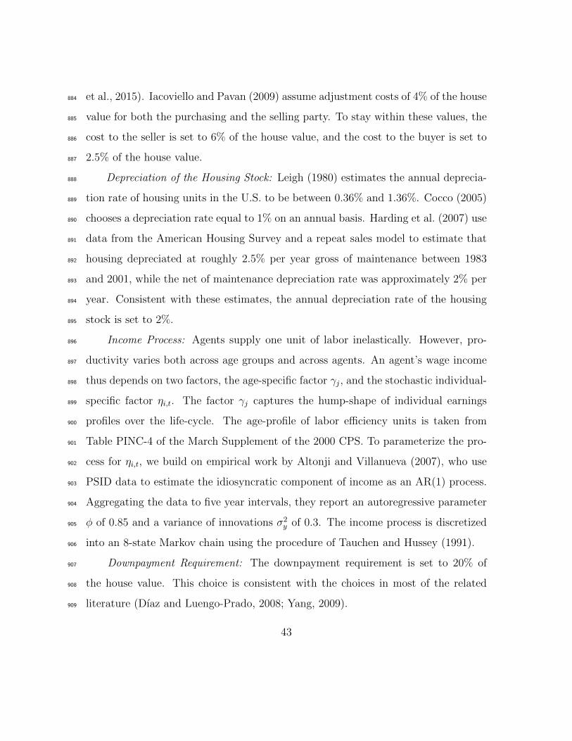
Depreciation of the Housing Stock: Leigh (1980) estimates the annual deprecia-888

tion rate of housing units in the U.S. to be between 0.36% and 1.36%. Cocco (2005)889

chooses a depreciation rate equal to 1% on an annual basis. Harding et al. (2007) use890

data from the American Housing Survey and a repeat sales model to estimate that891

housing depreciated at roughly 2.5% per year gross of maintenance between 1983892

and 2001, while the net of maintenance depreciation rate was approximately 2% per893

year. Consistent with these estimates, the annual depreciation rate of the housing894

stock is set to 2%.895

Income Process: Agents supply one unit of labor inelastically. However, pro-896

ductivity varies both across age groups and across agents. An agent’s wage income897

thus depends on two factors, the age-specific factor γj, and the stochastic individual-898

specific factor ηi,t. The factor γj captures the hump-shape of individual earnings899

profiles over the life-cycle. The age-profile of labor efficiency units is taken from900

Table PINC-4 of the March Supplement of the 2000 CPS. To parameterize the pro-901

cess for ηi,t, we build on empirical work by Altonji and Villanueva (2007), who use902

PSID data to estimate the idiosyncratic component of income as an AR(1) process.903

Aggregating the data to five year intervals, they report an autoregressive parameter904

φ of 0.85 and a variance of innovations σ2y of 0.3. The income process is discretized905

into an 8-state Markov chain using the procedure of Tauchen and Hussey (1991).906

Downpayment Requirement: The downpayment requirement is set to 20% of907

the house value. This choice is consistent with the choices in most of the related908

literature (Dıaz and Luengo-Prado, 2008; Yang, 2009).909

43

Housing Supply Elasticity: Parameterizing the housing production function is910

difficult. Empirical estimates of the price elasticity of housing supply vary widely.911

Blackley (1999) analyzes the real value of U.S. private residential construction put912

in place. She finds elasticities ranging from 0.8 to 3.7, depending on the dynamic913

specification of her model. Mayer and Somerville (2000) estimate a flow elasticity914

of 6, suggesting that a 10% increase in house prices will lead to a 60% increase in915

housing starts. Furthermore, price elasticities of housing supply vary widely within916

the United States. As argued by Glaeser et al. (2005), supply-side regulation (and917

thus the price elasticity of housing starts) differs by region and city. Some authors,918

such as Ortalo-Magne and Rady (2006), have hence chosen to fix the housing stock919

in their model. We take a different approach: In the baseline estimates, the housing920

production function is parameterized to fit a price elasticity of housing starts of921

ε = 2.5, which is roughly in the middle of the values estimated in the literature.922

As a robustness check, in Appendix D the results of the baseline estimation are923

compared to the model predictions obtained when setting ε = 6 and when setting924

ε = 0 (constant housing stock). This approach provides bounds on the impact of925

policy changes.926

Finally, Figure E.1 shows that the model is able to broadly match the pattern of927

homeownership rates over the life cycle seen in the data.928

[Locate Figure E.1 about here]929

References930

Altonji, J., Villanueva, E., 2007. The marginal propensity to spend on adult children.931

The B.E. Journal of Economic Analysis & Policy 7 (1).932

44

Attanasio, O., Browning, M., 1995. Consumption over the life cycle and over the933

business cycle. American Economic Review 85 (5), 1118–1137.934

Blackley, D., 1999. The long-run elasticity of new housing supply in the United935

States: empirical evidence for 1950 to 1994. The Journal of Real Estate Finance936

and Economics 18 (1), 25–42.937

Cocco, J., 2005. Portfolio choice in the presence of housing. Review of Financial938

Studies 18 (2), 535–567.939

Dıaz, A., Luengo-Prado, M., 2008. On the user cost and homeownership. Review of940

Economic Dynamics 11 (3), 584–613.941

Glaeser, E., Gyourko, J., Saks, R., 2005. Why have housing prices gone up? American942

Economic Review 95 (2), 329–333.943

Harding, J., Rosenthal, S., Sirmans, C., 2007. Depreciation of housing capital, main-944

tenance, and house price inflation: Estimates from a repeat sales model. Journal945

of Urban Economics 61 (2), 193–217.946

Iacoviello, M., Pavan, M., 2009. Housing and debt over the life cycle and over the947

business cycle. Boston College Working Papers in Economics.948

Jeske, K., Krueger, D., 2005. Housing and the macroeconomy: the role of implicit949

guarantees for government-sponsored enterprises. FRB Atlanta Working Paper950

Series 15.951

Leigh, W., 1980. Economic depreciation of the residential housing stock of the United952

States, 1950-1970. The Review of Economics and Statistics 62 (2), 200–206.953

45

Mayer, C., Somerville, C., 2000. Residential construction: Using the urban growth954

model to estimate housing supply. Journal of Urban Economics 48 (1), 85–109.955

Ortalo-Magne, F., Rady, S., 2006. Housing market dynamics: On the contribution956

of income shocks and credit constraints. The Review of Economic Studies 73 (2),957

459–485.958

Piazzesi, M., Schneider, M., Stroebel, J., 2015. Segmented housing search. Tech. rep.,959

National Bureau of Economic Research.960

Queisser, M., Whitehouse, E., 2005. Pensions at a glance: public policies across961

OECD countries. MPRA Paper 10907.962

Smith, L., Rosen, K., Fallis, G., 1988. Recent developments in economic models of963

housing markets. Journal of Economic Literature 26 (1), 29–64.964

Stroebel, J., Taylor, J. B., 2012. Estimated impact of the Federal Reserve’s mortgage-965

backed securities purchase program. International Journal of Central Banking966

8 (2), 1–42.967

Tauchen, G., Hussey, R., 1991. Quadrature-based methods for obtaining approximate968

solutions to nonlinear asset pricing models. Econometrica, 371–396.969

Yang, F., 2009. Consumption over the life cycle: How different is housing? Review970

of Economic Dynamics 12 (3), 423–443.971

46

Appendix B. Not for Publication: Analytical Appendix972

This appendix describes three analytical simplifications that help solving the973

model.974

Appendix B.1. Consumption-Renting Decision for Given House Size975

A significant simplification of the agents’ numerical problem can be achieved by976

first solving for two control variables in a static setting. For a given combination977

of state variables, savings choice, and housing choice, the allocation of resources978

between the consumption of the numeraire good and the consumption of housing979

services can be pinned down by a simple first-order condition.980

First, consider the problem of an agent who decides not to buy a house, but981

instead chooses to rent. For a given set of state variables and a given savings choice,982

the problem of how to allocate resources between consumption and housing services983

is static. Let the resources available for consumption and renting be denoted by X.984

The problem becomes:985

maxh

u(c, h)

(B.1)

s.t.: c+ prh ≤ X (B.2)

The optimal allocation of resources equates the marginal utility that can be derived986

from the two uses of funds, pruC = uH . Given the functional form for the utility987

function assumed in (1), this allows us to derive the demand for housing services988

(and thus the rental demand) for this particular agent as:989

h∗renter =θ

1− θc

pr= θ

X

pr(B.3)

47

Second, consider the case of an agent who chooses to buy a house of size h. For a990

given set of states and controls, we can again determine the resources available for991

consumption and housing services. For convenience, first calculate those resources992

for the hypothetical case where the agent decides to rent out their home completely.993

Again, denote those resources by X. This implies that the agent rents out the994

complete house and then uses the market to acquire the housing services she desires.995

Here, the problem is exactly analogous to the renter problem and the interior solution996

is then also given by (B.3).997

However, an agent with significant financial wealth who owns a small house might998

run into the constraint given by equation (2). In that case, the homeowner is trying999

to rent additional housing units which is not allowed by assumption. Hence, the1000

owners choice of housing services can be expressed as:1001

h∗owner = min

h, θ

X

pr

. (B.4)

Appendix B.2. Policy Alternatives in the Budget Constraint1002

For notational convenience, start with the case of no deductions. This is equiv-1003

alent to setting Ψ1 = Ψ2 = 0 in equation (14). That is, mortgage interest payments1004

cannot be deducted from the tax bill and the tax on rental income is levied both on1005

real rental income as well as on imputed rental income from owner-occupied housing.1006

It is important to note that the current U.S. policy is given by Ψ1 = Ψ2 = 1. For1007

both potential deductions considered in this paper, we illustrate the effect on the1008

agent’s budget constraint, both in the homeowner case and in the renter case. The1009

overall tax payments of each individual are also restricted so that they do not result1010

in a net subsidy.1011

To simplify notation, define the amount of resources to be spent on c and h as1012

48

X. This is analogous to Appendix B.1. The intra-temporal problem is then again1013

given by the maximization of period utility u(c, h) given the constraint c+ prh ≤ X.1014

Homeowner Case: In the absence of any deductions, the owner’s budget con-1015

straint can be written as follows, where T denotes the owner’s tax burden:1016

c+ s′ + ph+ AC + T =

pr(h− h) + (1 + r +mIs<0)s+ (1− τ ss)y + p(1− δ)h−1 + F(B.5)

For the homeowner, the amount of resources available for consumption and housing1017

services is thus given by:1018

X = prh+ (1 + r +mIs<0)s+ (1− τ ss)y + p((1− δ)h−1 − h)− T + F − s′ − AC

(B.6)

In terms of the model’s solution, the only effect of the policy alternatives is to alter1019

equation (B.2). The constraint becomes:1020

c+ prh−Ψ1 · (pr − δp)hτ r ≤ X −Ψ2 · rIs<0s (B.7)

c+ prh (1−Ψ1 · τ r) ≤ X −Ψ2 · rIs<0s (B.8)

The effective tax rate τ r is given by τ r · (1−δ ppr

). By defining the amount of effective1021

resources as X and the effective price of housing services for the owner as p, we can1022

use the exact same program to solve the intra-temporal problem for any combination1023

49

of policy alternatives.1024

X ≡ X −Ψ2 · rIs<0s (B.9)

p ≡ pr(1−Ψ1 · τ r

)(B.10)

c+ ph ≤ X (B.11)

Renter Case: The renter case can be derived analogously. For the renter, the1025

amount of available resources is given by:1026

Xr = (1 + r)s+ (1− τ ss)y + p ((1− δ)h−1)− T + F − s′ − AC (B.12)

Note that the mortgage interest rate deduction can apply to a renter, as the renter1027

can be a former homeowner who just sold her home and is paying off the mortgage1028

in the current period. Following the same steps as above and noting that deduction1029

Ψ1 does not apply, it can be shown that:1030

Xr ≡ Xr −Ψ2 · rIs<0s (B.13)

pr ≡ pr (B.14)

c+ prh ≤ X (B.15)

Appendix B.3. Voluntary Savings1031

In the numerical solution, we follow Yao and Zhang (2005) who define voluntary1032

savings instead of actual savings. In equation (8), the lower bound on savings, which1033

is equivalent to the maximum mortgage the agent can hold, depends on the value of1034

50

the house and is thus time-varying. Instead, define voluntary savings as:1035

b′ = s′ + (1− d)hp, (B.16)

so that whenever b′ is set equal to zero, the agent holds the maximum mortgage1036

allowed, (1 − d)hp. This formulation has the advantage of creating a rectangular1037

constraint set with c, b′, and h bounded below by zero. This makes the computational1038

solution on a grid significantly easier. It comes at the cost of having to carry the1039

previous period’s price as an additional state. A further downside of this formulation1040

is that it implies that mortgages involve margin calls and that negative home-equity1041

is not allowed.1042

References1043

Yao, R., Zhang, H., 2005. Optimal consumption and portfolio choices with risky1044

housing and borrowing constraints. Review of Financial Studies 18 (1), 197–239.1045

51

Appendix C. Not for Publication: Computational Appendix1046

This appendix outlines the steps taken to solve the model numerically.1047

Appendix C.1. State Space and Choice Variables:1048

Before describing our solution algorithm in more detail, it will be useful to define1049

the state space and control variables. An agent’s current state depends on four1050

individual variables: the housing stock h−1 and savings s at the beginning of the1051

period, the current realization of the persistent, idiosyncratic income shock η, and1052

the agent’s age j. An agent chooses whether to rent or buy, and in the latter case1053

how many housing units h to purchase. Other choice variables are savings s′ and the1054

amount of housing services consumed in the current period h.1055

The housing variable h can take a value of zero if the agent decides to rent,1056

and a value in the sethmin, hmin(1− δ)−1, hmin(1− δ)−2, . . .

if the agent decides1057

to be a homeowner. Restricting the housing choice to a delta-spaced housing grid is1058

a convenient assumption in the presence of fixed transaction costs. Appendix B.31059

introduced the concept of voluntary savings: b′ = s′ + (1− d)hp. This reformulation1060

of the model allows us to work with a rectangular constraint set, as the lower bound1061

on choices of b′ is always zero and thus independent of the housing choice. The1062

state variable b is approximated with a grid. Using the parameters of the estimated1063

autoregressive income process described in Section 5.1, we use a procedure introduced1064

by Tauchen and Hussey (1991) to discretize the income process with an eight-state1065

Markov process. As outlined in the discussion of the calibration in Section 5, the1066

model contains nine working cohorts and a group of retirees. Retired agents who1067

die are replaced with an equal measure of newborn agents, and the total measure1068

of agents is normalized to one. The relative size of the cohorts can thus be derived1069

from the retirees’ survival probability.1070

52

Appendix C.2. Calculation of Stationary Equilibria:1071

Stationary equilibria are calculated for a given policy regime and constant prices1072

and rents. We start with a reasonable guess of the level of lump-sum transfers. Given1073

those transfers and prices, we calculate optimal policies by solving an infinite horizon1074

problem for retirees using value function iteration. The resulting value function can1075

be used to solve the working cohorts’ problem backwards. Using the optimal policy1076

correspondence, we simulate the economy forward until a stationary distribution1077

of agents over the state space is achieved. We then check market clearing in the1078

housing and rental markets. The equilibrium prices are found using the nonlinear1079

optimization routine fminsearchcon for Matlab. In a last step, we adjust the level of1080

transfers and iterate until the government budget constraint clears as well.1081

To simplify the problem, we first calculate the resources available for consump-1082

tion of the nondurable numeraire good and housing services for all combinations of1083

states and remaining controls. That allows us to solve a simple static optimization1084

problem as outlined in Appendix B.1. Here, it is important to carefully consider1085

corner solutions. Using the optimal allocation of resources to those two uses, we cal-1086

culate the momentary utility flow for all possible choices and store those in a large1087

multidimensional object. The actual iteration on the value function is then simple1088

and fast. To further improve computational speed, we vectorize the problem such1089

that there is only a single maximization per iteration.1090

In the simulation, we store the exact distribution on the state-space grid. This1091

allows for a fast simulation routine given the Markov properties of both the exogenous1092

processes and the policy correspondences.1093

53

Appendix C.3. Solution Algorithm for Transitions:1094

For a given set of parameters and policy variables, we define the vector of market1095

clearing-equilibrium prices and government transfers as qt. This vector has three1096

elements: pt, prt , and Ft. Recall that Ωt captures the distribution of agents over age,1097

income, owned housing, and savings.1098

The algorithm for calculating the transition paths proceeds as follows. First,1099

guess the approximate length of the transition phase, T . Choosing a larger number1100

is computationally intensive, but ensures that transition can be achieved within the1101

number of periods considered. If transition can be achieved in a smaller number of1102

periods, the last transition periods will look very similar to the new steady state. In1103

our simulations, we choose a conservative T = 25, but find that the transition path1104

is not affected significantly for values of T greater than 15. After solving for the1105

stationary equilibria before and after the policy change that is considered, we know1106

the starting points q0 and Ω0 as well as the end points qT and ΩT . The algorithm1107

then iterates over the following steps:1108

1. Guess a sequence of qt for t = 1, ..., T − 1.1109

2. Solve backwards for the value functions given the guessed values qt. For exam-1110

ple, for period T − 1, it is easy to calculate VT−1 = max uT−1 +βVT given qT−11111

as VT is known in the new stationary equilibrium. Ignore distributions, since1112

we are not yet interested in market clearing.1113

3. Now solve forward: For period 1, find the market clearing q1, given V2 calcu-1114

lated in step 2 and Ω0. Also calculate Ω1. This gives the sequence of qt and Ωt1115

for t = 1, ..., T − 1.1116

4. Compare qt and qt. If not the same, replace qt by a weighted average of qt and1117

qt and return to step 2.1118

54

5. Compare ΩT with ΩT and increase T if the two distributions differ.1119

References1120

Tauchen, G., Hussey, R., 1991. Quadrature-based methods for obtaining approximate1121

solutions to nonlinear asset pricing models. Econometrica, 371–396.1122

55

Appendix D. Not for Publication: Robustness Appendix1123

The results in the main body of the paper are obtained using a price elasticity1124

of housing starts of ε = 2.5. As a robustness check, we also computed the results1125

for the model when the elasticity is ε = 6, and when the elasticity is ε = 0 (fixed1126

housing stock). These results are presented below.1127

Appendix D.1. Tax Credits1128

Table E.1 shows the welfare effects for the period immediately following the tax1129

credit for both the First-Time Homebuyer and the Repeat Homebuyer Tax Credits1130

under the various elasticities. The results in this table are calculated using the1131

steady state as the baseline for comparison. This differs from the approach taken in1132

the main body of the paper, where the welfare implications were computed relative1133

to a baseline in which a downpayment shock generated a boom-bust cycle in house1134

prices. We do this because the response of the economy to the downpayment shock,1135

and hence our baseline for computing the welfare, would be different for each value1136

of price elasticity. Computing the welfare effects relative to the steady state means1137

that all welfare effects are measured relative to a common baseline.1138

[Locate Table E.1 about here]1139

The results for the different housing supply elasticities show that independently1140

of the assumptions about ε, compensating all agents such that each is indifferent to-1141

wards the tax credit (lump-sum taxing winners and subsidizing losers) would involve1142

a net cost to the government. The tax credits therefore appear to have negative ag-1143

gregate welfare effects for the range of reasonable price elasticities of housing supply.1144

It is interesting to observe that for the First-Time Homebuyer Tax Credit, the1145

aggregate welfare effects are not monotone in the elasticity of housing supply. As1146

56

the elasticity increases, more initial homeowners and landlords suffer, since transfer1147

payments decline by a larger amount. In addition, for higher values of ε, the housing1148

stock rises more, reducing the value of existing housing assets by more and for a1149

longer period of time following the removal of the tax credit. Rents also decline by1150

more for higher values of ε, which hurts landlords. On the other hand, the larger fall1151

in rents explains why fewer initial renters lose as ε increases. In addition, since in1152

the high-elasticity economy house prices rise by the smallest amount, more renters1153

take advantage of the tax credit offered to them and become homeowners. This is1154

reflected in a larger increase in transaction volume in the high-elasticity economy1155

compared to the low-elasticity economy.1156

Appendix D.2. Tax on Imputed Rents1157

Table E.2 shows the price and quantity effects under various assumptions for1158

the housing supply elasticity on steady states when imputed rents are taxed. As1159

expected, the results show that with a more elastic housing supply the housing1160

stock declines by more. Consequently, house prices need to fall less to re-establish1161

equilibrium in the housing market. The smaller the price decrease, the larger the fall1162

in the homeownership rate resulting from the taxation of imputed rents.1163


Table E.3 shows the effect that taxing imputed rents has on welfare for the1165

various elasticity values, both between steady states and immediately following the1166

introduction. Interestingly, the number of agents losing in the new steady state is1167

increasing in the housing supply elasticity. The higher rents in high-ε economies1168

increase the tax burden due to the taxation of imputed rents for all agents. This1169

more than outweighs the lower capital losses for homeowners due to smaller price1170

57

declines in high-ε economies. On the other hand, relative to all homeowners, fewer1171

landlords lose in the high-ε state relative to the medium-ε state. While higher rents1172

increase the cost of owner-occupying due to the newly introduced tax, they also1173

increase the benefits of being a landlord. The low rents in the ε = 0 economy also1174

explain why the resources required to compensate losers are higher than in the ε = 2.51175

economy, despite the fact that fewer agents lose. In particular, the comparatively1176

rich landlords are significantly worse off in the zero-elasticity economy since both the1177

value of their housing stock and their rental income falls. Consequently, they require1178

a large consumption compensation to make them indifferent between staying in the1179

old steady state and switching with a similar agent in the new steady state.1180


In the low-ε economy, it is particularly the landlords that suffer more in the1182

immediate aftermath of the policy change than in a comparison of steady states.1183

This is due to the initial decline in rents.1184

Appendix D.3. No Mortgage Interest Deductions1185

Table E.4 shows the price and quantity effects in the steady state under the vari-1186

ous elasticity values when no mortgage interest deductions are allowed. Again, with1187

a higher elasticity, the price of housing declines by less due to the larger adjustments1188

in the quantity of the housing stock. The other prices and quantities in the model1189

are relatively unaffected by the elasticity choice.1190


Table E.5 shows the effect that removing mortgage interest deductions has on1192

welfare for the various elasticity values, both between steady states and immediately1193

58

following the change in policy. Unlike in the previous experiment, the percentage of1194

agents who lose in the new steady state is decreasing in ε. The number of owner-1195

occupiers and landlords who lose declines because prices fall by less in the higher-ε1196

economy, reducing the capital loss faced by homeowners.16 In addition to the price1197

effect, as the elasticity increases, rents increase by more following the reform, reducing1198

the number of landlords who are worse off as a result of this policy change.1199


16In the previous experiment, this effect was outweighed by the increasing cost of the tax on imputedrents.

59

Appendix E. Figures and Tables for Appendices1201

Figure E.1: Homeownership Rate for Different Age Groups

20 25 30 35 40 45 50 55 60 650

10

20

30

40

50

60

70

80

90

100

Per

cent

Age

ModelData

Note: Data for the homeownership rate by age (solid blue line) comes from

the U.S. Statistical Abstract for 2005, Table 957. We take the average

homeownership rate for the year 2000. The model line (dashed red line)

shows the homeownership rate when the model is in the baseline steady

state.

60

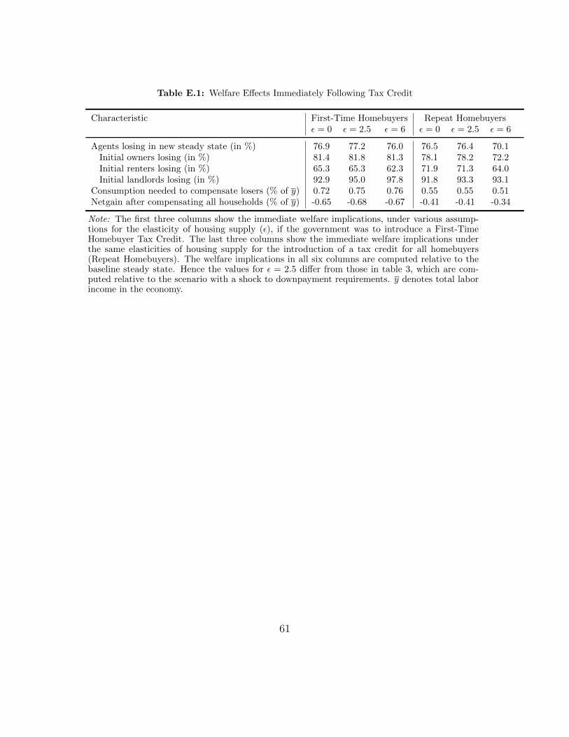
Table E.1: Welfare Effects Immediately Following Tax Credit

Characteristic First-Time Homebuyers Repeat Homebuyersε = 0 ε = 2.5 ε = 6 ε = 0 ε = 2.5 ε = 6

Agents losing in new steady state (in %) 76.9 77.2 76.0 76.5 76.4 70.1Initial owners losing (in %) 81.4 81.8 81.3 78.1 78.2 72.2Initial renters losing (in %) 65.3 65.3 62.3 71.9 71.3 64.0Initial landlords losing (in %) 92.9 95.0 97.8 91.8 93.3 93.1

Consumption needed to compensate losers (% of y) 0.72 0.75 0.76 0.55 0.55 0.51Netgain after compensating all households (% of y) -0.65 -0.68 -0.67 -0.41 -0.41 -0.34

Note: The first three columns show the immediate welfare implications, under various assump-tions for the elasticity of housing supply (ε), if the government was to introduce a First-TimeHomebuyer Tax Credit. The last three columns show the immediate welfare implications underthe same elasticities of housing supply for the introduction of a tax credit for all homebuyers(Repeat Homebuyers). The welfare implications in all six columns are computed relative to thebaseline steady state. Hence the values for ε = 2.5 differ from those in table 3, which are com-puted relative to the scenario with a shock to downpayment requirements. y denotes total laborincome in the economy.

61

Table E.2: Quantity and Price Effects in Steady State — Tax on Imputed Rents

Moment of Interest Baseline ε = 0 ε = 2.5 ε = 6

House Price (normalized) 1.00 0.85 0.96 0.98Rental Price (normalized) 1.00 0.90 1.00 1.02Price-Rent Ratio 21.66 20.63 20.68 20.68

Housing Stock (normalized) 1.000 1.000 0.896 0.875Rental Market (normalized) 1.000 2.697 2.604 2.566Homeownership Rate (in %) 72.3 43.2 39.9 39.3Share of Landlords (in %) 18.6 17.8 21.5 22.1Average LTV (in %) 29.5 7.9 7.6 8.1

Transfers (% of y) 38.57 41.61 41.45 41.43Tax Loss: mortgage interest deduction 0.48 0.13 0.13 0.14Tax Loss: non-taxed imputed rents 1.77 0.00 0.00 0.00

Note: The table shows moments of interest in the baseline steady state as well asthe steady state for the model with taxes on imputed rents (Ψ1 = 0) under variousassumptions for the elasticity of housing supply (ε). y denotes total labor income in theeconomy.

62

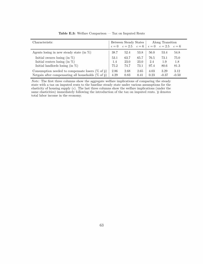
Table E.3: Welfare Comparison — Tax on Imputed Rents

Characteristic Between Steady States Along Transitionε = 0 ε = 2.5 ε = 6 ε = 0 ε = 2.5 ε = 6

Agents losing in new steady state (in %) 38.7 52.4 53.8 56.0 53.4 54.8

Initial owners losing (in %) 53.1 63.7 65.7 76.5 73.1 75.0Initial renters losing (in %) 1.4 23.0 23.0 2.4 1.9 1.8Initial landlords losing (in %) 75.2 74.7 73.1 97.4 80.6 81.3

Consumption needed to compensate losers (% of y) 2.86 2.68 2.65 4.03 3.29 3.12Netgain after compensating all households (% of y) 4.29 0.83 0.41 0.23 -0.37 -0.50

Note: The first three columns show the aggregate welfare implications of comparing the steadystate with a tax on imputed rents to the baseline steady state under various assumptions for theelasticity of housing supply (ε). The last three columns show the welfare implications (under thesame elasticities) immediately following the introduction of the tax on imputed rents. y denotestotal labor income in the economy.

63

Table E.4: Quantity and Price Effects in Steady State — No Mortgage Interest Deductions

Moment of Interest Baseline ε = 0 ε = 2.5 ε = 6

House Price (normalized) 1.00 0.97 0.99 1.00Rental Price (normalized) 1.00 1.00 1.02 1.03Price-Rent Ratio 21.66 21.06 21.02 21.02

Housing Stock (normalized) 1.000 1.000 0.982 0.977Rental Market (normalized) 1.000 1.788 1.756 1.732Homeownership Rate (in %) 72.3 57.7 57.5 57.4Share of Landlords (in %) 18.6 19.7 19.9 20.1Average LTV (in %) 29.5 15.0 15.3 15.3

Transfers (% of y) 38.57 39.86 39.83 39.84Tax Loss: mortgage interest deduction 0.48 0.00 0.00 0.00Tax Loss: non-taxed imputed rents 1.77 1.57 1.57 1.58

Note: The table shows moments of interest in the baseline steady state as well as thesteady state for the model with no mortgage interest deductions (Ψ2 = 0) under variousassumptions for the elasticity of housing supply (ε). y denotes total labor income in theeconomy.

64

Table E.5: Welfare Comparison — No Mortgage Interest Deductions

Characteristic Between Steady States Along Transitionε = 0 ε = 2.5 ε = 6 ε = 0 ε = 2.5 ε = 6

Agents losing in new steady state (in %) 27.7 17.8 17.4 31.9 33.6 32.7

Initial owners losing (in %) 29.5 15.8 15.2 43.2 37.4 36.0Initial renters losing (in %) 23.0 23.0 23.0 2.4 23.9 23.9Initial landlords losing (in %) 73.2 25.0 23.9 86.0 77.6 75.6

Consumption needed to compensate losers (% of y) 0.11 0.10 0.11 0.51 0.36 0.31Netgain after compensating all households (% of y) 2.70 2.20 2.15 1.23 1.21 1.19

Note: The first three columns show the aggregate welfare implications of comparing the steadystate with a tax on no mortgage interest deductions to the baseline steady state under variousassumptions for the elasticity of housing supply (ε). The last three columns show the welfareimplications (under the same elasticities) immediately following the removal of mortgage interestdeductions. y denotes total labor income in the economy.

65

appendix a. not for publication: calibration...

Documents