Appendix A

Functions, Functionals and their Derivatives

A.1 Functions and Functionals

The usage of variables and functions in this book will be familiar to most readers, but some of the techniques used for analysis of functionals may be unfamiliar. As a preamble to the description of functionals, first we describe the terminology for the simpler cases. The following is not intended as a rigorous or comprehensive introduction but simply a clarification of the terminology used here.

A variable is a symbol used to represent an unspecified value of a set. The va-lue of the variable is one particular member of the set and the range is the set itself. For example, the variable x might represent a real number. In this case, the range is the set of real numbers from to , and in a particular instance, the value of x may be the number 3.81.

A function of one variable associates a value from one set (the range of the function) with each value from another set (the domain of the function). For example, the function 23y x expresses y as a function of the variable x. If the domain of the function (i. e. the range of its argument x) is the set of real num-bers, then the resulting range of the function y will be the set of non-negative real numbers. The variable y is called the dependent variable or value of the function, and x is the independent variable or the argument of the function.

If the specific form of a function is not given, then it is written in the form y f x , or y y x . The concept is simply extended to functions of several arguments, e. g. 1 2 3, ,y y x x x . The arguments may be vectorial or tensorial rather than scalar, as may be the dependent variable.

A functional is loosely defined as a “function of a function”. It is a function in which one or more of the arguments is itself a function. The range of the func-tional may be either another function or just a variable. A functional is distin-guished here from a function by use of square brackets . Thus, for instance, z z y , where y y x .

306 Appendix A Functions, Functionals and their Derivatives

It is sometimes necessary to make a careful distinction between the function f itself and its value at a particular value of x, which we shall denote f x . In this regard, we follow the more usual convention, but note that in some subjects, it is common to use f x for the function and f for its value.

A.2 Some Special Functions

Throughout this book, we need to make much use of some special functions, principally related to absolute values and certain singularities. We denote the absolute value by , 0x x x ; , 0x x x . We use the following notation for the Macaulay bracket: , 0x x x ; 0, 0x x .

We also need the derivatives of the above functions. They may be loosely de-fined as follows, although more formal definitions are provided by the subdif-ferential, which is introduced in Appendix D on convex analysis. For the time being, we define a modified signum function as S 1, 0x x , S 1, 0x x , and S x as undefined for 0x , but within the range 1 S 0 1 . Note that this does not correspond to the conventional signum function, usually denoted by “sgn” or “sg”, and which is usually defined by sgn 0 0 .

We define the Heaviside step function as 1

H S 12

x x , so that

H 0, 0x x , H 1, 0x x , and H x is undefined for 0x , but within the range 0 H 0 1 .

We define the Dirac impulse function x through the relationship

0 0

b

a

x x f x dx f x , 0a x b . It can be proven straightforwardly that

H x x , where f x denotes the differential of f x . The quantity that plays the same role as the absolute value for a symmetrical

second-order tensor is kl klx x , and we define the derivative of this with respect to ijx as a generalised tensorial signum function, which we write

Sij

ij ijkl kl

xx

x x. Like the signum function of a scalar, this quantity is unde-

fined when 0kl klx x (which necessarily occurs only when 0ijx ), but we

require S 0 S 0 1ij ij .

It is emphasised again that some of the above definitions can be set in a much more satisfactory formalism by the use of convex analysis; see Appendix D.

A.3 Derivatives and Differentials 307

A.3 Derivatives and Differentials

The derivative of a function is the instantaneous rate of change of the function

with respect to one of its arguments. The definition of the derivative df

f xdx

of the function f x with respect to x should be familiar:

0

limx

f x x f xf x

x (A.1)

The above is of course the fundamental definition from which many familiar expressions for derivatives of particular functions are obtained.

When the function has more than one argument, partial derivatives are de-fined by obtaining the derivative with respect to one argument whilst consider-ing the others as constants. Thus if ,f f x y the partial derivative

,xff x y

x with respect to x is defined as:

0

, ,, limx

x

f x x y f x yf x y

x (A.2)

In the main text, the differential of an integral is required. If

,b x

a x

F x f x t dt , then application of the basic definitions results in

, ,b x

a x

f db daF x dt f x b f x a

x dx dx (A.3)

The differential of a function f x is defined by df f x dx , where dx is an independent variable. (Note the formal distinction, often ignored, between a differential and a derivative). The total differential of a function of more than one argument, for example ,f x y , is defined in the following way:

f fdf dx dy

x y (A.4)

where each of the terms of the form f

dxx

is a partial differential.

The concept of the differential of a function can be extended to that of a func-tional by using either the Gateaux or Frechet differential, and these are devel-oped as follows.

308 Appendix A Functions, Functionals and their Derivatives

In the classical calculus of variations, the variation of a functional f u is de-fined in terms of a variation u of its argument function:

0

, limf u u f u

f u u (A.5)

where is a scalar. A more precise statement defining f is based on a choice of norm in the space of f:

0

lim , 0f u u f u

f u u (A.6)

For sufficiently well-behaved functionals, f will be a linear functional of its argument u, so that , ,f u u f u u , for all scalars , and

1 2 1 2, , ,f u u u f u u f u u , for all 1u and 2u . In this case, the functional f may be presented as the operation of a linear operator f u on the function u, which we write in the following way:

, , ,uf u u f u u f u u (A.7)

Note that the above expression does not represent simply the inner product of f u and u, although in certain simple cases, it does take this form. The linear operator f u above is known as the Gateaux derivative of the func-tional f. An alternative basic definition for the generalised derivative of f (the Frechet derivative) requires that f be that linear operator satisfying

0

,lim 0u

f u u f u f u u

u (A.8)

where the norms are defined in some appropriate way. It can be shown that the Gateaux and Frechet definitions are equivalent when

the linear operator f is continuous in the function u, and so we shall simply refer to f in this book as the Frechet derivative. It is not essential to retain the variational notation in the definition of the Frechet derivative; therefore, a varia-tion u can be replaced by any fixed v. Furthermore, when this variation is re-placed by the differential du, the resulting functional , ,df u du f u du will

be referred to as the Frechet differential. Frechet derivatives are used in this book to define Legendre transformations of functionals (see Appendix C), and Frechet differentials are used in deriving the incremental response of material behaviour.

A.4 Selected Results 309

A.4 Selected Results

A.4.1 Frechet Derivatives of Integrals

Although the Frechet derivative is defined for general functionals, here we are interested principally in functionals of the form,

ˆˆ ˆ ˆ,f u f u w d (A.9)

where Y is the domain of and f is a continuously differentiable function of the variable u , which is in turn a function of . Here and in the main text, we adopt the convention that any quantity which is a function of is denoted by a ‘hat’ notation, e. g. w .

Then, according to definitions (A.7) and (A.8), one can show that the Frechet differential of the functional (A.9) is given by

ˆ ˆ,

ˆ ˆ ˆ ˆ ˆ ˆ, ,ˆ

f udf u du f u du du w d

u (A.10)

Now consider a more general case in which there are several independent variables: 1 1

ˆˆ ˆ ˆ ˆ ˆ,N Nf u u f u u w d , where f is a continu-

ously differentiable function of functional variables iu , 1i N . When the variable u in (A.7) and (A.8) is identified as the full N-dimensional

space of functions ˆiu , then the Frechet differential is

1

1

ˆ ˆ ˆ ,ˆ ˆ ˆ ˆ ˆ ˆ, ,

NN

iii

f u udf u du f u du du w d

u (A.11)

For the definition of partial Legendre transformations, the variable u in defi-nition (A.7) and (A.8) is identified as an n-dimensional subspace of the full N-dimensional space of functions ˆiu . In this case, the corresponding Frechet derivative is given by the following operator f , which is linear in any integrable functions iv :

1

1

ˆ ˆ ˆ ,ˆ ˆ ˆ ˆ,

ˆ

nN

iii

f u uf u v v w d

u (A.12)

310 Appendix A Functions, Functionals and their Derivatives

A.4.2 Frechet Derivatives of Integrals Containing Differential Terms

Now consider the case where the integral contains differential terms. It is

straightforward to show that the Frechet differential of ˆ

ˆb

a

duf u d

d with

respect to the function u is given by ˆ

ˆ ˆ ˆ,b

ba

a

dvf u v d v

d. Similarly, the

Frechet differential of 2

2

ˆˆ

b

a

d uf u d

d with respect to the function u is given by

2

2

ˆ ˆˆ ˆ,

bb

aa

d v dvf u v d

dd.

It is straightforward to show that the Frechet differential of 2ˆ1ˆ

2

b

a

duf u d

d with respect to the function u is given by

ˆ ˆˆ ˆ,

b

a

du dvf u v d

d d. Integrating by parts, we obtain

2

2

ˆ ˆˆ ˆ ˆ ˆ,

b b

a a

du d uf u v v vd

d d (A.13)

The latter form proves convenient in some applications.

Similarly, the Frechet differential of

22

2

ˆ1ˆ2

b

a

d uf u d

d with respect to the

function u is given by 2 2

2 2

ˆ ˆˆ ˆ,

b

a

d u d vf u v d

d d. Integrating by parts twice, we

obtain

2 3 4

2 3 4

ˆ ˆ ˆ ˆˆ ˆ ˆ ˆ,

b b b

aa a

d u dv d u d uf u v v vd

dd d d (A.14)

where again this latter form again proves convenient in some applications.

Appendix B

Tensors

B.1 Tensor Definitions and Identities

A second-order Cartesian tensor a is also written ija or in matrix form for

three dimensions as 11 12 13

21 22 23

31 32 33

a a a

a a a

a a a

. We use the summation convention over

a repeated index; thus, for instance, 11 22 33kka a a a and 3

1ij jk ij jk

j

a a a a .

Alternatively, we may write 2ij jka a a . The unit tensor, or Kronecker is

defined by 1,ij i j ; 0,ij i j . A tensor is symmetric if it is equal to its

transpose ij jia a and is antisymmetric, or skew-symmetric, if ij jia a . The

inverse of a tensor or matrix is defined by 1ij jk ika a , and a tensor or matrix is

orthogonal if its inverse is equal to its transpose ij jk ika a .

The tensor has principal values 1a , 2a , 3a , which are the eigenvalues of the

matrix, and are the solutions of the cubic equation,

3 21 2 3 0a a I aI I (B.1)

where 1I , 2I , 3I are the invariants of the tensor, which are

1 1 2 3triiI a a a aa (B.2)

22

2

1 2 2 3 3 1

1 1tr tr

2 2ij ji ii jjI a a a a

a a a a a a

a a (B.3)

312 Appendix B Tensors

3

33 21 2 3

12 3

61

2tr 3tr tr tr det6

ij jk ki ij ji kk ii jj kkI a a a a a a a a a

a a aa a a a a (B.4)

Note that some authors define 2I with the opposite sign, but we prefer the

notation used here; otherwise, 2J (see below), which plays a major role in the

analysis of shear behaviour, is always negative. The traces of the powers may alternatively be chosen as defining the three invariants,

1 2 3 1tr iia a a a Ia (B.5)

2 2 2 2 21 2 3 2 1tr 2ij jia a a a a I Ia (B.6)

3 3 3 3 31 2 3 3 2 1 1tr 3 3ij jk kia a a a a a I I I Ia (B.7)

The deviator of a tensor is defined as follows:

1

3ij ij kk ija a a (B.8)

so that 1 tr 0I a . The second and third invariants of the deviator are also

often required and may be written in a variety of forms:

2 2

22 22 1

2 2 21 2 3 1 2 2 3 3 1

2 221 2 2 3 3 1

1 1 1

2 2 61 1 1

tr tr2 3 3

1

31

6

ij ji ij ji ii jjI J a a a a a a

I I

a a a a a a a a a

a a a a a a

a a (B.9)

3 3

33 2 33 2 1 1

1 2 3 2 3 1 3 1 2

3 3 31 2 3

2 2 21 2 3 2 3 1 3 1 2 1 2 3

1 1 2

3 3 9

1 1 2 1 2tr tr tr tr

3 3 9 3 27

12 2 2

271

227

3 12

ij jk ki ij jk ki ij ji kk ii jj kkI J a a a a a a a a a a a a

I I I I

a a a a a a a a a

a a a

a a a a a a a a a a a a

a a a a

(B.10)

B.2 Mixed Invariants 313

B.2 Mixed Invariants

The four mixed invariants of two tensors can be written as:

1 1 2 2 3 3ij jitr a b a b a b a bab (B.11)

2 2 2 21 1 2 2 3 3ij jk kitr a a b a b a b a ba b (B.12)

2 2 2 21 1 2 2 3 3ij jk kitr a b b a b a b a bab (B.13)

2 2 2 2 2 2 2 21 1 2 2 3 3ij jk kl litr a a b b a b a b a ba b (B.14)

where the forms expressed in terms of the principal values only apply if the principal axes coincide for the two tensors. Thus for two tensors, there are 10 invariants, three for each tensor alone and four mixed invariants.

B.2.1 Differentials of Invariants of Tensors

Since the various potentials used in this book are most often written in terms of invariants and then are differentiated to obtain the constitutive behaviour, it is convenient to note the differentials of tensors and their invariants given in Table B.1.

314 Appendix B Tensors

Table B.1. Differentials of functions of tensors and their invariants

f ijdf da

kla ki lj

kla 1

3ki lj ij kl

1I ij

2I 1ji ija I

3I 1 2jk ki ji ija a a I I

2J 1

1

3ji ji ija a I

3J 2jk ki ija a J

tr a ij

2tr a 2 jia

3tr a 3 jk kia a

tr ab jib

2tr a b 2 jk kia b

2tr b a jk kib b

2 2tr a b 2 jk kl lia b b

Appendix C

Legendre Transformations

C.1 Introduction

The Legendre transformation is one of the most useful in applied mathematics, although its role is not always explicitly recognised. Well-known examples in-clude the relation between the Lagrangian and Hamiltonian functions in analyti-cal mechanics, between strain energy and complementary energy in elasticity theory, between the various potentials that occur in thermodynamics, and be-tween the physical and hodograph planes occurring in the theories of the flow of compressible fluids and perfectly plastic solids. The Legendre transformation plays a central role in the general theory of complementary variational and ex-tremum principles. Sewell (1987) presents a comprehensive account of the the-ory from this viewpoint with particular emphasis on singular points. These transformations have also been widely employed in rate formulations of elas-tic/plastic materials to transfer between stress-rate and deformation-rate poten-tials, e. g. Hill (1959, 1978, 1987); Sewell (1987). These applications are rather different from those used in this book. We review therefore those basic proper-ties of the transformation that are needed in the main text.

C.2 Geometrical Representation in (n + 1)-dimensional Space

A function ( )iZ X x , 1i n , defines a surface in 1n -dimensional , iZ x space. However, the same surface can be regarded as the envelope of

tangent hyperplanes. One way of describing the Legendre transformation is that it allows one to construct the functional representation that describes Z in terms of these tangent hyperplanes. This relationship is a well-known duality in ge-ometry. The gradients of the function iX x are denoted by iy :

ii

Xy

x (C.1)

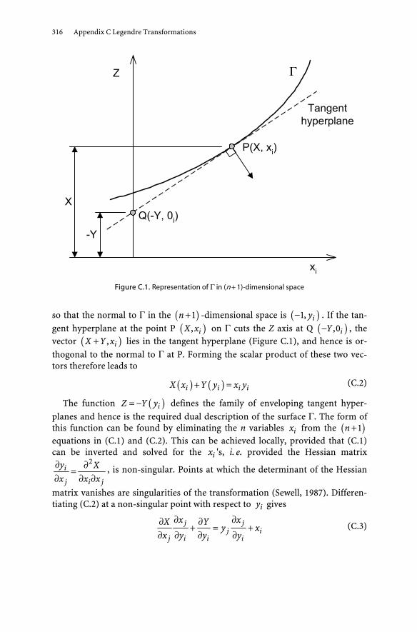
316 Appendix C Legendre Transformations

Tangenthyperplane

Z

xi

Q(-Y, 0i)

P(X, xi)

-Y

X

Figure C.1. Representation of in (n + 1)-dimensional space

so that the normal to in the 1n -dimensional space is 1, iy . If the tan-gent hyperplane at the point P , iX x on cuts the Z axis at Q ,0iY , the vector , iX Y x lies in the tangent hyperplane (Figure C.1), and hence is or-thogonal to the normal to at P. Forming the scalar product of these two vec-tors therefore leads to

i i i iX x Y y x y (C.2)

The function iZ Y y defines the family of enveloping tangent hyper-planes and hence is the required dual description of the surface . The form of this function can be found by eliminating the n variables ix from the 1n equations in (C.1) and (C.2). This can be achieved locally, provided that (C.1) can be inverted and solved for the ix 's, i. e. provided the Hessian matrix

2i

j i j

y Xx x x

, is non-singular. Points at which the determinant of the Hessian

matrix vanishes are singularities of the transformation (Sewell, 1987). Differen-tiating (C.2) at a non-singular point with respect to iy gives

j jj i

j i i i

x xX Yy x

x y y y (C.3)

C.3 Geometrical Representation in n-dimensional Space 317

which, by virtue of (C.1) reduces to

ii

Yx

y (C.4)

Relations (C.1)–(C.3) define the Legendre transformation. This transforma-tion is self-dual because, if the function iZ Y y is used to define a surface

“pointwise” in , iZ y space, then iZ X x describes the same surface “planewise” because 1, ix define the normal to and X is the intercept of the tangent plane with the Z axis from (C.2).

The transformation is not in general straightforward to perform analytically. An exception is when ( )iX x is a quadratic form, 1

2( )i ij i jX x A x x , where ijA is

a non-singular, symmetrical matrix. Hence, the dual variables are

i ij ji

Xy A x

x, so that 1

i ij jx A y , and the Legendre dual is also a quadratic

form:

1 1 11 12 2i i i i ij i j ij i j ij i jY y x y X x A y y A y y A y y (C.5)

The transformation in general is succinctly written

ii

Xy

x (C.1)bis

i i i iX x Y y x y (C.2)bis

ii

Yx

y (C.4)bis

The choice of the sign of the dual function is somewhat arbitrary, and Y is sometimes written instead of Y. The choice is usually governed by physical con-siderations.

C.3 Geometrical Representation in n-dimensional Space

An alternative geometrical visualisation in n-dimensional space is also valuable in gaining understanding of formal results.

For fixed C but variable ix , the relation

, 0i i i i ix y X x x y C (C.6)

defines a family of hyperplanes in n-dimensional iy space. These hyperplanes envelope a surface in this space, the equation of which is obtained by eliminat-ing the ix between (C.4) and

0ii i

Xy

x x (C.7)

318 Appendix C Legendre Transformations

On comparison with (C.1) and (C.2), it follows that the equation of this sur-face is iY y C , so that the hyperplanes defined by (C.4) envelope the level surfaces of the dual function Y. Dually, the hyperplanes defined by

,i i i i ix y Y y x y C (C.8)

envelope the level surfaces of iX x in ix space. These level surfaces are, of course, the “cross sections” of the 1n -dimensional surfaces iZ X x and

iZ Y y discussed above.

C.4 Homogeneous Functions

Of particular importance in applications in continuum mechanics are cases where the function iZ X x is homogeneous of degree p in the ix 's, so that

i iX x pX x for any scalar . From Euler's theorem for such functions, it follows that

i i i ii

XpX x x x y

x (C.9)

so that from (C.2),

i i i ii

YqY y x y y

y (C.10)

where 1 1

1p q

, so that the Legendre dual iY y is necessarily homogeneous

of degree 1

pq

p.

In the example above, 2p , so that X and Y are both homogeneous of degree two. A familiar example of this situation is in linear elasticity where the elastic strain energy ijE and the complementary energy ijC are both quadratic

functions of their argument and satisfy the fundamental relation,

ij ij ij ijE C (C.11)

Another case of particular importance in rate-independent plasticity theory occurs when X is homogeneous and of degree one, so that i i iX x x y , in which case the dual function iY y is identically zero from (C.2). There is a simple geometric interpretation of this far-reaching result. Since

i iX x X x , the 1n -dimensional surface iZ X x is a hypercone with its vertex at the origin. Hence, all tangent hyperplanes meet the Z axis at

0Z , so that 0iY y for all iy . This special case is pursued further later,

C.5 Partial Legendre Transformations 319

and the terminology of convex analysis will prove particular useful in its treat-ment (see Appendix D).

C.5 Partial Legendre Transformations

Now suppose that the functions depend on two families of variables, ,i iX x say, where ix and i are n- and m-dimensional vectors, respectively. We can perform the Legendre transformation with respect to the ix variables as above and obtain the dual function ,i iY y . The variables i play a passive role in this transformation and are treated as constant parameters. Hence, the three basic equations are now

, ,i i i i i iX x Y y x y (C.12)

ii

Xy

x and i

i

Yx

y (C.13)

If the derivatives of X with respect to the passive variables i are denoted by

i , then it follows from (C.12) that

ii i

X Y (C.14)

It is also possible, in general, to perform a Legendre transformation on ,i iX x with respect to the i variables and construct a second dual function ,i iV x with the properties,

, ,i i i i i iX x V x (C.15)

where

ii

X , ii

V (C.16)

and furthermore:

ii i

X Vy

x x (C.17)

since now the ix 's are the passive variables. This process can be continued. A Legendre transformation of ,i iY y with

respect to the i variables produces a fourth function ,i iW y . The same function is obtained by transforming ,i iV x with respect to the ix variables. A closed chain of transformation is hence produced as shown in Figure C.2, where the basic differential relations are summarised. The best known example

320 Appendix C Legendre Transformations

of such a closed chain of transformations is in classical thermodynamics, where the four functions are the internal energy ,u s v , the Helmholtz free energy

,f v , the Gibbs free energy ,g p , and the enthalpy ,h s p , where , s, v, and p are the temperature, entropy, specific volume, and pressure respectively, e. g. Callen (1960). Other examples are given by Sewell (1987).

C.6 The Singular Transformation

When X is homogeneous of order one in ix , so that , ,i i i iX x X x , the value of /i iy X x is unaffected by the transformation i ix x , and so the mapping from i ix y is 1 . Furthermore, since

,i i i ix y X x (C.18)

the dual function ,i iY y is identically zero, as already noted above, and so

0i ii i

Y YdY dy d

y (C.19)

But also from (C.13),

i i i i i ii i

X Xx dy y dx dx d

x (C.20)

ii

ii

iiX

xXy

xX

,

),(

ii

ii

iiY

yYx

yY

,

),(

ii

ii

iiW

xWx

yW

,

),(

ii

ii

iiV

xVy

xV

,

),(

ii yxYX

iiWY W V x yi i

iiXV

X Y W V 0

Figure C.2. Chain of four partial Legendre transformations

C.7 Legendre Transformations of Functionals 321

which by virtue of (C.1) reduces to

0i i ii

Xx dy d (C.21)

Hence, by comparing (C.19) with (C.21), it follows that

ii

Yx

y and

i i

X Y (C.22)

where is an undetermined scalar, reflecting the non-unique nature of this sin-gular transformation.

The above development is classical in the sense that all the functions are as-sumed to be sufficiently smooth for all derivatives to exist. In practice, the sur-faces encountered in plasticity theory, on occasion, contain flats, edges, and corners. Such surfaces and the functions defining them can be included in the general theory using some of the concepts of convex analysis. In particular, the commonly defined derivative is replaced by the concept of a “subdifferential”, and the simple Legendre transformation is generalised to the “Legendre-Fenchel transformation” or “Fenchel dual”. For simplicity of presentation, we have so far used the classical notation, and convex analysis is introduced in Appendix D. Treatments of the mechanics of elastic/plastic materials that use convex analysis notation may be found in Maugin (1992), Reddy and Martin (1994), and notably Han and Reddy (1999).

Because our main concern here is to exhibit the overall structure of the theory as it affects the developments of constitutive laws, we have not highlighted the behaviour of any convexity properties of the various functions under the trans-formations. These considerations are very important for questions of unique-ness, stability, and the proof of extremum principles, which are beyond the scope of this book, but are fruitful areas for future research. Some of these as-pects of Legendre transformations are considered at length in the book by Sewell (1987).

C.7 Legendre Transformations of Functionals

C.7.1 Integral Functional of a Single Function

Consider a functional,

ˆˆ ˆ ˆ,X x X x w d (C.23)

where Y is the domain of and X is a continuously differentiable function of a functional variable x .

322 Appendix C Legendre Transformations

If ˆ ˆ ,

ˆˆ

X xy

x, then the Legendre transform of the function X is

ˆ ˆˆ ˆ ˆ ˆ, ,Y y x y X x (C.24)

It follows from the standard properties of the transform that ˆ ˆ ,

ˆˆ

Y yx

y.

The functional defined by

ˆˆ ˆ ˆ ˆ ˆ ˆ ˆ,Y y Y y w d x y w d X x (C.25)

may then be considered the Legendre transform of the original functional, and using definitions of Appendix A, it can be confirmed that this definition satisfies the appropriate differential conditions.

C.7.2 Integral Functional of Multiple Functions

A case of interest in the present work is a Legendre transform of a functional of the form,

ˆˆ ˆ ˆ ˆ ˆ, , ,X x u X x u w d (C.26)

where X is a continuously differentiable function of the variables x and u .

Denoting ˆ ˆ ˆ, ,

ˆˆ

X x uy

x, the Legendre transform of the function

X with respect to the variable x is defined as

ˆ ˆˆ ˆ ˆ ˆ ˆ ˆ, , , ,Y y u x y X x u (C.27)

From the standard properties of the transform, it follows that

ˆ ˆ ˆ, ,

ˆˆ

Y y ux

y (C.28)

ˆ ˆˆ ˆ ˆ ˆ, , , ,

ˆ ˆ

Y y u X x u

u u (C.29)

Then, the Legendre transformation of functional (C.26) in function x , where function u is a passive variable, is given by the functional,

ˆˆ ˆ ˆ ˆ ˆ ˆ ˆ ˆ ˆ ˆ, , , ,Y y u Y y u w d x y w d X x u (C.30)

C.7 Legendre Transformations of Functionals 323

and using definitions of Appendix A, it can be confirmed that this definition satisfies the appropriate differential conditions.

When x is not a function but a variable, denoted x, all above equations are valid, except that Equation (C.30) may be rewritten as

ˆˆ ˆ ˆ ˆ, , , ,Y y u Y y u w d xy X x u (C.31)

where

ˆ , ,

ˆX x u

y w dx

(C.32)

When the function X is a continuously differentiable function of the func-tion x (or variable x) and any finite number N of functions iu , the same Equa-tions (C.27)–(C.30) are still valid, except that Equation (C.29) unfolds into N equations:

1 1ˆ ˆˆ ˆ ˆ ˆ ˆ ˆ ˆ, , , , ,

, 1ˆ ˆ

N N

i i

Y y u u X x u y ui N

u u (C.33)

C.7.3 The Singular Transformation

An important case in rate-independent plasticity theory occurs when functional ˆ ˆ ˆ, ,X x u in (C.26) is homogeneous of degree one in, say, x :

ˆ ˆˆ ˆ ˆ ˆ, , , ,X x u X x u (C.34)

From Euler’s theorem, it follows that

ˆ ˆ ˆ, ,ˆ ˆ ˆ ˆ ˆ ˆ, ,

ˆ

X x uX x u x y x

x (C.35)

Then the Legendre transformation of the function ˆ ˆ ˆ, ,X x u with re-

spect to u , when other variables and functions are passive, is defined by Equation (C.27), so that after substitution of (C.35), we obtain

ˆ ˆˆ ˆ ˆ ˆ ˆ ˆ, , , , 0Y y u x y X x u (C.36)

The properties of this transformation are

ˆ ˆ ˆ, ,ˆˆ

ˆ

Y y xx

y (C.37)

ˆ ˆˆ ˆ ˆ ˆ, , , ,ˆ

ˆ ˆ

X x u Y y u

u u (C.38)

324 Appendix C Legendre Transformations

where ˆ is an undetermined scalar, reflecting the non-unique nature of this singular transformation.

Then the Legendre transformation of functional (C.26) in function x , when function u is a passive variable, is given by the functional,

ˆˆ ˆ ˆ ˆ ˆ ˆ ˆ ˆ ˆ ˆ, , , , 0Y y u Y y u w d x y w d X x u (C.39)

and using definitions of Appendix A, it can be confirmed that this definition satisfies the appropriate differential conditions.

Appendix D

Convex Analysis

D.1 Introduction

The terminology of convex analysis allows a number of the issues relating to hyperplastic materials to be expressed succinctly. In particular, through the definition of the subdifferential, it allows rigorous treatment of functions with singularities of various sorts. These arise, for instance, in the treatment of the yield function. A brief summary of some basic concepts of convex analysis is given here. The terminology is based chiefly on that of Han and Reddy (1999). A more detailed introduction to the subject is given by Rockafellar (1970). No attempt is made to provide rigorous, comprehensive definitions here. For a fuller treatment, reference should be made to the above texts. Although it is currently used by only a minority of those studying plasticity, it seems likely that in time convex analysis will become the standard paradigm for expressing plas-ticity theory.

D.2 Some Terminology of Sets

We use brackets to indicate a set, so that 0, 1, 3.5 is simply a set contain-ing the numbers 0, 1 and 3.5. A closed set containing a range of numbers is de-noted by , , thus ,a b x a x b , where the meaning of the contents of the final bracket is “x, such that a x b ”. We use to denote the null (empty) set.

In the following, C is a subset in a normed vector space V (in simple terms a space in which a measure of distance is defined), usually with the dimension of

nR (with n finite), but possibly infinite dimensional. The notation , is used for an inner product, or more generally the action of a linear operator on a func-tion. The space V is the space dual to V under the inner product *,x x , so

326 Appendix D Convex Analysis

that x V and *x V . More generally, V is termed the topological dual space of V (the space of linear functionals on V).

The operation of summation of two sets, illustrated in Figure D.1a, is defined by

1 2 1 2 1 1 2 2,C C x x x C x C (D.1)

The operation of scalar multiplication of a set, illustrated in Figure D.1b is de-fined by

C x x C (D.2)

It is also convenient to define the operation of multiplication of a set C by a set S of scalars:

,SC x S x C (D.3)

The definitions of the interior and boundary of a set are intuitively simple concepts, but their formal definitions depend first on the definition of distance. In nR , the Euclidian distance is defined as

1 2, ,d x y x y x y x y (D.4)

and we define the open ball of radius r and centered at ox as

, ,o oB x r x d x x r (D.5)

The interior of C is then defined as

int 0, ,C x B x C (D.6)

C

C

x2

x1

(a) (b)

Figure D.1. (a) Summation of sets; (b) scalar multiple of a set

D.3 Convex Sets and Functions 327

This means that there exists some (possibly very small) so that a ball of ra-dius is entirely contained in C. The closure of C is defined as the intersection of all sets obtained by adding a ball of non-zero radius to C:

cl 0, 0,C C B (D.7)

Finally, the boundary of C is that part of the closure of C that is not interior:

bdy cl \ intC C C (D.8)

D.3 Convex Sets and Functions

A set C is convex if and only if

1 x y C , ,x y C , 0 1 (D.9)

where, for instance, ,x y C means “for all x and y belonging to C”. Simple examples of convex and non-convex sets in two-dimensional space are given in Figure D.2. A function f whose domain is a convex subset C of V and whose range is real or is convex if and only if

1 1f x y f x f y , ,x y C , 0 1 (D.10)

This is illustrated for a function of a single variable in Figure D.3. Convexity requires that NP NQ for all N between X and Y. This property has to be true for all pairs of X,Y within the domain of the function. A function is strictly con-vex if can be replaced by < in (D.10) for all x y .

The effective domain of a function is defined as the part of the domain for which the function is not; thus, dom f x x V f x .

Figure D.2. Non-convex and convex functions

328 Appendix D Convex Analysis

x

z

Q

P

YNX(1- )

z = f(x)

x + (1- )y= x + (1- )y

Figure D.3. Graph of a convex function of one variable

D.4 Subdifferentials and Subgradients

The concept of the subdifferential of a convex function is a generalisation of the concept of differentiation. It allows the process of differentiation to be extended to convex functions that are not smooth (i. e. continuous and differentiable in the conventional sense to any required degree). If V is a vector space and V is its dual under the inner product , , then *x V is said to be a subgradient of

the function f x , x V , if and only if *,f y f x x y x , y .

The subdifferential, denoted by f x , is the subset of V consisting of all vectors *x satisfying the definition of the subgradient:

* *, ,f x x V f y f x x y x y (D.11)

For a function of one variable, the subdifferential is the set of the slopes of li-nes passing through a point on the graph of the function, but lying entirely on or below the graph. The concept is illustrated in Figure D.4.

The concept of the subdifferential allows us to define “derivatives” of non-differentiable functions. For example, the subdifferential of w x is the signum function, which we now define as a set-valued function:

1 , 0

S 1, 1 , 0

1 , 0

x

x w x x

x

(D.12)

D.5 Functions Defined for Convex Sets 329

x

w

w = f(x)

P

Figure D.4. Subgradients of a function at a non-smooth point

Thus at a point x, f x may be a set consisting of a single number equal to f x , or a set of numbers, or (in the case of a non-convex function) may be

empty.

D.5 Functions Defined for Convex Sets

The indicator function of a set C is a convex function defined by

0,

,Cx C

I xx C

(D.13)

so that the indicator function is simply zero for any x that is a member of the set and elsewhere. Although this appears at first sight to be a rather curious function, it proves to have many applications. In particular, it plays an impor-tant role in plasticity in that it is closely related to the yield function.

The normal cone CN x of a convex set C is the set-valued function defined by

* *, 0,CN x x V x y x y C (D.14)

330 Appendix D Convex Analysis

It is straightforward to show that 0CN x if intx C (the point is in the interior of the set), that CN x can be identified geometrically with the cone of normals to C at x if bdyx C (the point is on the boundary of the set), and further that CN x is empty if x C (the point is outside the set). Furthermore, the subdifferential of an indicator function of any convex set is the normal cone of that set: C CI x N x .

Another important function defined for a convex set is the gauge function or Minkowski function, defined for a set C as

inf 0C x x C (D.15)

where inf x denotes the infimum, or lowest value of a set. In other words, C x is the smallest positive factor by which the set can be

scaled, and x is a member of the scaled set. The meaning is most easily under-stood for sets that contain the origin (which proves to be the case for all sets of interest in hyperplasticity). In the following, we shall therefore assume that C is convex and contains the origin. It is straightforward to see in this case that

1C x for any point on the boundary of the set, is less than unity for a point inside the set, and is greater than unity for a point outside the set. At the origin,

0 0C . In the context of (hyper)plasticity, it is immediately obvious that the gauge

may be related to the conventional yield function. If the set C is the set of (gen-eralised) stresses that are accessible for any given state of the internal variables (the elastic region), then the yield function is a function conventionally taken as zero at the boundary of this set (the yield surface), negative within, and positive without. One possible expression for the yield function would therefore be

1Cy . Other functions could of course be chosen as the yield func-tion, but this is perhaps the most rational choice; so we follow Han and Reddy (1999) in calling this the canonical yield function. To emphasise the case where the yield surface is written in this way, we shall give it the special notation

1Cy . The gauge function is always homogeneous of order one in its argument x, so

that C Cx x . (In the language of convex analysis, such functions are simply referred to as positively homogeneous.) The canonical yield function is therefore conveniently written in the form of a positively homogeneous function of the (generalised) stresses, minus unity. It is also clear that the gauge of the set of accessible generalised stresses contains exactly the same information as the yield function, canonical or otherwise, and there may be benefits from specify-ing the gauge rather than the yield function.

It is useful to note that at the boundary of C, the normal cone can also be written , 0C C CN x I x x . This proves to be a convenient form that allows the normal cone to be expressed in terms of the subdifferential of the gauge function and therefore (in hyperplasticity), of the canonical yield function.

D.6 Legendre-Fenchel Transformation 331

It is straightforward to see that the definition (D.15) can be inverted. Given a positively homogeneous function f x , one can define a set C, such that f x is the gauge function of C:

1C x f x (D.16)

which has the property that C x f x . It is worth noting, too, that the indi-cator function of a set containing the origin can always be expressed in the fol-lowing form, and this proves useful in the application of convex analysis to (hy-per)plasticity:

,0 1C CI x I x (D.17)

The function ,0I x is simply zero for all non-positive values of x and

for positive values.

D.6 Legendre-Fenchel Transformation

The Legendre-Fenchel transformation (often simply called the Fenchel dual, or conjugate function) is a generalisation of the concept of the Legendre transfor-mation. If f x is a convex function defined for all x V , its Legendre-Fenchel transformation is * *f x , where *x V is defined by

* * sup *,x V

f x x x f x (D.18)

where supx V

means the supremum, or highest value for any x V .

It is straightforward to show the Fenchel dual is a generalisation of the Leg-endre transform. We use the notation that if *x f x and * *f x is the Fenchel dual of f x , then * *x f x .

Some useful Fenchel duals, together with their subdifferentials are given in Table D.1. The dual of the sum of two functions involves the process of infimal convolution:

f infy V

g x f x y g y (D.19)

Table D.1 also includes some special functions that are defined in Section D.10.

332 Appendix D Convex Analysis

Table D.1. Some Fenchel duals and their subdifferentials

f x f x * *f x * *f x

0I x 0N x 0 0

,0I x ,0N x

0, *I x 0, *N x

1,1I x 1,1N x *x S *x

0,1I x 0,1N x *x H *x

pos x H x ,0 * 1I x ,0 * 1N x

1 0 0 *I x 0 *N x

x 1 1 *I x 1 *N x

2 2x x 2* 2x *x

nx , 1n 1nnx

1*1

n nxn

n

1 1* nx

n

expx expx * log * *x x x log *x

f x g x f x g x *f * *g x

f ax a f ax * *f x a 1* *f x a

a

D.7 The Support Function

The support function is also defined for a convex set. For a convex set C in V, if *x V , then the support function is defined by

* sup , *C x x x x C (D.20)

Note that although C is a set of values of the variable x, the argument of the support function is the variable *x conjugate to x.

It can be shown that the support function is the Fenchel dual of the indicator function. The support function is always homogeneous of order one in *x , i. e. it is positively homogeneous.

It follows that any homogeneous order-one function defines a set in dual space. In hyperplasticity, one can observe that the dissipation function is homo-geneous and order one in the internal variable rates. It can thus be interpreted as a support function, and the set it defines in the dual space of generalised stresses is the set of accessible generalised stress states (the elastic region). The Fenchel dual of the dissipation function is the indicator function for this set of accessible states, which is zero throughout the set. We can identify this indicator function

D.7 The Support Function 333

with the Legendre transform w y of the dissipation function introduced in Chapter 4.

Equation (D.20) can be inverted to obtain the set C from the support func-tion. If * *f x is a homogeneous first-order function in *x , then the set de-fined by solving the system of inequalities,

, * * * , *C x x x f x x (D.21)

satisfies the condition that * * *C x f x . Application of (D.21), with * *f x as the dissipation function, allows the set of accessible (generalised)

stresses to be derived from the dissipation function in a systematic manner; hence the elastic region can be derived from the dissipation function.

The subdifferential of the support function defines a set called the maximal responsive map (see Han and Reddy, 1999, although we depart from their nota-tion here):

* *C Cx x (D.22)

The normal cone and the maximal responsive map are inverse in the sense that

* *C Cx x x N x (D.23)

It also follows [see Lemma 4.2 of Han and Reddy (1999)] that C is simply re-lated to the support function by the subdifferential at the origin, i. e. the maxi-mal responsive map at the origin. Thus

0 0C CC (D.24)

Both the gauge and support functions are positively homogeneous. Defining the domain of the support function dom *CS x , it can be shown (see Han

and Reddy, 1999) that

0 *

*,sup

*CCx S

x xx

x (D.25)

and C x is called the polar of *C x , written C C . The process is

symmetrical so that C C and, defining the domain of the gauge function dom CG x ,

0

*,* supC

Cx G

x xx

x (D.26)

Further, we have the following inequality:

* *, , * ,C Cx x x x x S x G (D.27)

334 Appendix D Convex Analysis

and the equality holds for *Cx x :

* *, , * , *C C Cx x x x x x x S (D.28)

Application of (D.25), together with 1Cy , allows the canonical yield function to be determined directly from the dissipation function.

D.8 Further Results in Convex Analysis

Whilst the above are the most important results needed in Chapter 13, it is worth noting some further relationships between convex sets and functions.

The polar C of a convex set C is defined as

* * 1CC x x (D.29)

in other words, it is the set for which the support function of C is the gauge. The polar f of a non-negative convex function f, which is zero at the origin,

is defined by

* inf 0 , * 1 ,f x x x f x x (D.30)

and it can be shown that Equations (D.25) and (D.26) can be derived from this more general relationship.

Finally, the indicator and the gauge of a convex set are said to be obverse to each other, where the obverse g of a function f is defined by

inf 0 1g x f x (D.31)

and the operation 1f x f x is called right scalar multiplication [note

that 00f x I x if f x and 0f x f x if f x ].

D.9 Summary of Results for Plasticity Theory

In summary, we have the following concepts from convex analysis which are of relevance in plasticity theory:

A convex set C in V. The indicator function CI x of the set. The gauge function C x of the set. The support function *C x , which is the Fenchel dual of the indicator, and

is also the polar of the gauge function. The normal cone C CN x I x which is a set in V which is the subdiffer-

ential of the indicator function.

D.9 Summary of Results for Plasticity Theory 335

The maximal responsive map, which is the subdifferential of the support function * *C Cx x .

The set C is the subdifferential of the support function at the origin 0 0C CC .

The relationships among these quantities are illustrated in Figure D.5 for the simple one-dimensional set ,C a b .

The roles of these concepts in hyperplasticity are explored in more detail in Chapter 11, but Table D.2 gives the correspondences among some concepts in conventional plasticity theory and in the convex analytical approach.

Table D.2 Correspondences between conventional plasticity theory and the convex analytical approach

Conventional plasticity theory

Convex analytical approach to (hyper)plasticity

Elastic region A convex set in (generalised) stress space.

Yield surface The indicator function or (for some purposes) the gauge function, or equivalently the canonical yield function.

Plastic potential and flow rule

Gauge function (or equivalently the canonical yield func-tion) and the normal cone.

Plastic work Support function (equal to the dissipation function). NB: For models in which energy can be stored through plastic straining, this is not equal to plastic work.

The indicator of the elastic region and the support func-tion (dissipation) are Fenchel duals.

(No equivalents in con-ventional theory)

The gauge function of the elastic region and the support function (dissipation) are polars.

336 Appendix D Convex Analysis

xNxIx CC*

xIC

xC

** xxx CC

*xC

baC ,

*xIC

baC 1,1

Figure D.5. Relationships among functions of a convex set in one dimension

D.10 Some Special Functions

We have already introduced the signum function (D.12), which we treat as a set-valued function. Closely related is the Heaviside step function:

0 , 0

1H S 1 0, 1 , 0

21 , 0

x

x x x

x

(D.32)

D.10 Some Special Functions 337

It is also useful to define a closely related set-valued function:

, 0

H , 1 , 0

1 , 0

x

x x

x

(D.33)

H x , which can also be written as 0,N x , is useful because it is the sub-

differential of the positive values of x, defined as

, 0

pos, 0

xx

x x (D.34)

Note that careful distinction is needed among pos x , the absolute value x , and the Macaulay bracket x . Note that all of these functions are convex.

References

Atkinson, J.H., Richardson, D. and Stallebrass, S.E. (1990) Effect of recent stress history on the stiffness of overconsolidated soil, Géotechnique, Vol. 40, No. 4, 531 540

Bazant, Z.P. (1978) Endochronic inelasticity and incremental plasticity, Int. J. Solids Struct., Vol. 14, 691 714

Berryman, J.G. (1980) Confirmation of Biot’s Theory, Applied Physics Letters, Vol 37, 382 384 Borja, R.I., Tamagnini, C. and Amorosi, A. (1997) Coupling plasticity and energy-conserving elastic-

ity models for clays, Proc. ASCE, J. Geotechnical Eng., Vol. 123, No. 10, 948 956 Butterfield, R. (1979) A natural compression law for soils (an advance on e-log p'), Géotechnique,

Vol. 29, No. 4, 469 480 Callen, H.B. (1960) Thermodynamics, Wiley, New York Collins, I.F. (2002) Associated and non-associated aspects of the constitutive laws for coupled elas-

tic/plastic materials, Int. J. Geomechanics, Vol. 2, No. 2, 259 267 Collins, I.F. (2003) A systematic procedure for constructing critical state models in three dimensions,

Int. J. Solids Struct., Vol. 40, No. 17, 4379 4397 Collins, I.F. and Hilder, T. (2002). A theoretical framework for constructing elastic/plastic constitu-

tive models of triaxial tests, Int. J. Numer. Anal. Methods Geomech., Vol. 26, 1313 1347 Collins, I.F. and Houlsby, G.T. (1997) Application of thermomechanical principles to the modelling

of geotechnical materials, Proc. R. Soc. London, Series A, Vol. 453, 1975 2001 Collins, I.F. and Kelly, P. A. (2002) A thermomechanical analysis of a family of soil models, Géotech-

nique, Vol. 52, No. 7, 507 518 Collins, I.F. and Muhunthan, B. (2003) On the relationship between stress-dilatancy, anisotropy, and

plastic dissipation for granular materials, Géotechnique, Vol. 53, No. 7, 611 618 Coussy, O. (1995) Mechanics of porous continua, Wiley, New York Dafalias, Y.F. and Herrmann, L.R., (1982) Bounding surface formulation of soil plasticity, in G.N.

Pande and O.C. Zienkiewicz (eds.), Soil mechanics: Transient and cyclic loads, Wiley, New York, 253 282

de Borst, R. (1986) Non-linear Analysis of Frictional Materials, Doctoral thesis, Delft University of Technology

Drucker, D.C. (1951) A more fundamental approach to plastic stress-strain relations, Proc. 1st U.S. Nat. Congr. Appl. Mech. ASME, June, 487 491

Drucker, D.C. (1959) A definition of a stable inelastic material, J. Appl. Mech., Vol 26, 101 106 Einav, I (2002) Applications of thermodynamical approaches to mechanics of soils, PhD Thesis,

Technion – Israel Institute of Technology, Haifa Einav, I. (2004) Thermomechanical relations between stress-space and strain-space models,

Géotechnique, Vol. 54, No. 5, 315 318 Einav, I. (2005) Energy and variational principles for piles in dissipative soil, Géotechnique, Vol. 55,

No. 7, 515–525

340 References

Einav, I. and Puzrin, A.M. (2003) Evaluation of continuous hyperplastic critical state (CHCS) model, Géotechnique, Vol. 53, No. 10, 901 913

Einav, I. and Puzrin, A.M. (2004a) Pressure-dependent elasticity and energy conservation in elasto-plastic models for soils, J. Geotechnical Geoenvironmental Eng., Vol. 130, No. 1, 81 92

Einav, I. and Puzrin, A.M. (2004b), Continuous hyperplastic critical state (CHCS) model: derivation, Int. J. Solids Struct., Vol. 41, No. 1, 199 226

Einav, I., Puzrin, A.M., and Houlsby, G.T. (2003a) Numerical studies of hyperplasticity with single, multiple and a continuous field of yield surfaces, Int. J. Numer. Anal. Methods Geomechanics, Vol. 27, No. 10, 837 858

Einav, I., Puzrin, A.M., and Houlsby, G.T. (2003b) Continuous hyperplastic models for overconsoli-dated clays, Mathematical and Computer Modelling, special issue on Mathematical Models in Geomechanics, Proc. Symp. at Scilla di Reggio Calabria, Sept. 19–22, 2000, Vol. 37, Nos. 5/6, 515 523

Eringen, A.C. (1962) Nonlinear theory of continuous media, McGraw-Hill, New York Fleming, W.G.K., Weltman, A.J., Randolph, M.F. and Elson, W.K. (1985) Piling engineering, Surrey

University Press Fung, Y.C (1965) Foundations of solid mechanics, Prentice-Hall, New Jersey Gajo, A. and Muir Wood, D. (1999) A kinematic hardening constitutive model for sands: The multi-

axial formulation, Int. J. Numer. Anal. Methods Geomechanics, Vol. 23, No. 9, 925 965 Graham, J. and Houlsby, G.T. (1983) Elastic anisotropy of a natural clay,. Géotechnique, Vol. 33, No.

2, June, 165 180; corrigendum: Géotechnique, 33(3), Sept. 1983, 354 Han, W. and Reddy, B.D. (1999) Plasticity: Mathematical theory and numerical analysis, Springer,

New York Hill, R. (1959) Some basic principles in the mechanics of solids without a natural time, J. Mech. Phys.

Solids, Vol. 7, 209 225 Hill, R. (1978) Aspects of invariance in solid mechanics, Adv. Appl. Mech., Vol. 18, 39 63 Hill, R. (1981) Invariance relations in thermoelasticity with generalised variables, Math. Proc. Cam-

bridge Philos. Soc., Vol. 90, 373 384 Hill, R. (1987) Constitutive dual potentials in classical plasticity, J. Mech. Phys. Solids, Vol. 35, 23 33 Holzapfel, G.A. (2000) Nonlinear solid mechanics, Wiley, Chichester Houlsby, G.T. (1979) The work input to a granular material, Géotechnique, Vol. 29, No. 3, 354 358 Houlsby, G.T. (1981) A study of plasticity theories and their applicability to soils, PhD Thesis, Uni-

versity of Cambridge Houlsby, G.T. (1982) A derivation of the small-strain incremental theory of plasticity from ther-

momechanics, Proc. Int. Union Theor. Appl. Mech. (IUTAM) Conf. Deformation and Flow of Granular Materials, Delft, Holland, August 28-30, 109 118

Houlsby, G.T. (1985) The use of a variable shear modulus in elastic-plastic models for clays, Comput. Geotechnics, Vol. 1, 3 13

Houlsby, G.T. (1986) A general failure criterion for frictional and cohesive materials, Soils Found., Vol. 26, No. 2, 97 101

Houlsby, G.T. (1992) Interpretation of dilation as a kinematic constraint, Proc. Workshop on Modern Approaches to Plasticity, Horton, Greece, June 12 16, 19 38

Houlsby, G.T. (1996) Derivation of incremental stress-strain response for plasticity models based on thermodynamic functions, Proc. Int. Union Theor. Appl. Mech. (IUTAM) Symp. Mech. Granu-lar Porous Mater., Cambridge, July 15 17, Kluwer, 161 172

Houlsby, G.T. (1997) The work input to an unsaturated granular material, Géotechnique, Vol. 47, No. 1, 193 196

Houlsby, G.T. (1999) A model for the variable stiffness of undrained clay, Proc. Int. Symp. Pre-Failure Deformation Soils, Torino, September 26 29, Balkema, Vol. 1, 443 450

Houlsby, G.T. (2000) Critical state models and small-strain stiffness, Developments in Theoretical Geomechanics, Proc. Booker Memorial Symp., Sydney, November 16 17, Balkema, 295 312

References 341

Houlsby, G.T. (2002) Some mathematics for the constitutive modelling of soils, Proc. Conf. Math. Methods Geomechanics, Horton, Greece, Advanced Mathematical and Computational Geome-chanics, ed. D. Kolymbas, Springer, 35 53

Houlsby, G.T. Amorosi, A., and Rojas, E. (2005) Elastic moduli of soils dependent on pressure: a hyperelastic formulation, Géotechnique, Vol. 55, No. 5, June, 383 392

Houlsby, G.T. and Cassidy, M.J. (2002) A plasticity model for the behaviour of footings on sand under combined loading, Géotechnique, Vol. 52, No. 2, March, 117 129

Houlsby, G.T, Cassidy, M.J., and Einav, I. (2005) A generalised Winkler model for the behaviour of shallow foundations, Géotechnique, Vol. 55, No. 6, 449 460

Houlsby, G.T and Mortara, G. (2004) A continuous hyperplasticity model for sands under cyclic loading, Proc. Int. Conf. Cyclic Behav. Soils Liquefaction Phenomena, Bochum, Germany, March 31 April 2, 21 26

Houlsby, G.T. and Puzrin, A.M. (1999) An approach to plasticity based on generalised thermody-namics, Proc. Int. Symp. Hypoplasticity, Horton, Greece, 233 245

Houlsby, G.T. and Puzrin, A.M. (2000) A thermomechanical framework for constitutive models for rate-independent dissipative materials, Int. J. Plasticity, Vol. 16, No. 9, 1017 1047

Houlsby, G.T. and Puzrin, A.M. (2002) Rate-dependent plasticity models derived from potential functions, J. Rheol., Vol. 46, No. 1, Jan./Feb., 113 126

Houlsby, G.T. and Wroth, C.P. (1991) The variation of the shear modulus of a clay with pressure and overconsolidation ratio, Soils Found., Vol. 31, No. 3, Sept., 138 143

Hueckel, T. (1977) The flow law of the granular solids with variable unloading rule, Problemes de la Rheologie et de Mecanique des Sols, ed. W. K. Nowacki, PWN Warsaw, 203 217

Il’iushin, A.A. (1961) On the postulate of plasticity, J. Appl. Math. Mech., Vol. 25, No. 3, 746 752 Iwan, W.D. (1967) On a class of models for the yielding behaviour of continuous and composite

systems, J. Appl. Mech., Vol. 34, 612 617 Kavvadas, M.J. and Amorosi, A. (1998) A plasticity approach for the mechanical behaviour of struc-

tured soils, The geotechnics of hard soils – soft rocks, ed. Evangelista and Picarelly, Balkema, Rotterdam, 603 612

Kolymbas, D. (1977) A rate-dependent constitutive equation for soils, Mech. Res. Commun., Vol. 4, 367 372

Lam, N.-S. and Houlsby, G.T. (2005) The theoretical modelling of a suction caisson foundation using hyperplasticity theory, Proc. Int. Symp. Frontiers Offshore Geotechnics, Perth, Australia, Sept.

Lemaitre, J. and Chaboche, J.-L. (1990) Mechanics of solid materials, Cambridge University Press Likitlersuang, S. (2003) A hyperplasticity model for clay behaviour: An application to Bangkok clay,

DPhil Thesis, Oxford University Likitlersuang, S. and Houlsby, G.T. (2006) Development of hyperplasticity models for soil mechan-

ics, Int. J. Num. and Anal. Meht. in Geomechanics, Vol. 30, No. 3, 229 254 Martin, C.M. and Houlsby, G.T. (2001) Combined loading of spudcan foundations on clay: Numeri-

cal modelling, Géotechnique, Vol. 51, No. 8, Oct., 687 700 Martin, J.B. and Nappi, A. (1990) An internal variable formulation for perfectly plastic and linear

hardening relations in plasticity, Eur. J. Mech., A/Solids, Vol. 9, No. 2, 107 131 Matsuoka, H. and Nakai, T. (1974) Stress-deformation and strength characteristics of soil under

three different principal stresses, Proc. JSCE, Vol. 232, 59 70 Maugin, G.A. (1992) The thermomechanics of plasticity and fracture, Cambridge University Press Maugin, G.A. (1999) The thermodynamics of nonlinear irreversible processes, World Scientific, Sin-

gapore Mitchell, J.K. (1976) Fundamentals of soil behaviour, Wiley, New York Mróz, Z. (1967) On the description of anisotropic work hardening, J. Mech. Phys. Solids, Vol. 15,

163 175 Mróz, Z., Norris, V.A., and Zienkiewicz, O.C. (1979). Application of an anisotropic hardening model

in the analysis of elasto-plastic deformation of soil, Géotechnique, Vol. 29, No. 1, 1 34

342 References

Mróz, Z. and Norris, V.A. (1982) Elastoplastic and viscoplastic constitutive models for soils with application to cyclic loading, Soil mechanics – transient and cyclic loads, ed. G.N. Pande and O.C. Zienkiewicz, Wiley, 173 218

Owen, D.R.J. and Hinton, E. (1980) Finite Elements in Plasticity: Theory and Practice, Pineridge Press, Swansea

Palmer, A.C. (1966) A limit theorem for materials with non-associated flow laws, J. Mécanique, Vol. 5, No. 2, 217 222

Pappin, J.W. and Brown S.F. (1980) Resilient stress-strain behaviour of a crushed rock, Int. Symp. Soils under Cyclic Transient Loading, Swansea, 169 177

Prager, W. (1949) Recent developments in the mathematical theory of plasticity, J. Appl. Phys., Vol. 20, 235 241

Prevost, J.H. (1978) Plasticity Theory for Soil Stress-Strain Behaviour, Proc.ASCE, J. Eng. Mech. Div, Vol. 104, No EM5, 1177 1197

Puzrin, A.M. and Burland J.B. (1996) A logarithmic stress-strain function for rocks and soils, Géotechnique, Vol. 46, No. 1, 157 164

Puzrin, A.M. and Burland J.B. (1998) Non-linear model of small-strain behaviour of soils, Géotech-nique, Vol. 48, No. 2, 217 233

Puzrin, A.M. and Burland, J.B. (2000) Kinematic hardening plasticity formulation of small strain behaviour of soils, Int. J. Numer. Anal. Methods Geomechanics, Vol. 24, No. 9, 753 781

Puzrin, A.M. and Houlsby, G.T. (2001a) On the non-intersection dilemma, Géotechnique, Vol. 51, No. 4, 369 372

Puzrin, A.M. and Houlsby, G.T. (2001b) Fundamentals of kinematic hardening hyperplasticity, Int. J. Solids Struct., Vol. 38, No. 21, May, 3771 3794

Puzrin, A.M. and Houlsby, G.T. (2001c) A thermomechanical framework for rate-independent dissipative materials with internal functions, Int. J. Plasticity, Vol. 17, 1147 1165

Puzrin, A.M. and Houlsby, G.T. (2003) Rate dependent hyperplasticity with internal functions, Proc. ASCE, J. Eng. Mech. Div., Vol. 129, No. 3, March, 252 263

Puzrin, A.M., Houlsby, G.T., and Burland, J.B. (2001) Thermomechanical formulation of a small strain model for overconsolidated clays, Proc. R. Soc. London, Series A, Vol. 457, No. 2006, Feb., 425 440

Puzrin, A.M. and Kirshenboim, E. (1999) Evaluation of a small strain model for overconsolidated clays, Proc. Conf. Pre-failure Deformation Characteristics Geomaterials, Torino, Vol. 1, Balkema, Rotterdam, 483 490

Rampello, S., Viggiani, G.M.B., and Amorosi, A. (1997) Small-strain stiffness of reconstituted clay compressed along constant triaxial stress ratio paths, Géotechnique, Vol. 47, No. 3, 475 489

Reddy, B.D. and Martin, J.B. (1994) Internal variable formulations of problems in elastoplasticity: constitutive and algorithmic aspects, Appl. Mech. Rev., Vol. 47, No. 9, 429 456

Rockafellar, R.T. (1970) Convex analysis, Princeton University Press, New Jersey Roscoe, K.H. and Burland, J.B. (1968) On the generalised behaviour of ‘wet’ clay, Engineering plastic-

ity, ed. Heyman, J. and Leckie, F.A., Cambridge University Press, 535 610 Rouainia, M. and Muir Wood, D. (1998) A kinematic hardening model for structured clays, The

geotechnics of hard soils – soft rocks, ed. Evangelista and Picarelly, Balkema, Rotterdam, 817 824

Schofield, A.N and Wroth, C.P. (1968) Critical state soil mechanics, McGraw-Hill, London Sewell, M.J (1987) Maximum and minimum principles, Cambridge University Press Shaw, P. and Brown, S.F. (1988) Behaviour of granular materials under repeated load biaxial and

triaxial stress conditions, Géotechnique, Vol. 38, No. 4, 627 634 Stallebrass, S.E. and Taylor, R.N. (1997) The development and evaluation of a constitutive model for

the prediction of ground movements in overconsolidated clay, Géotechnique, Vol. 47, No. 2, 235 254

Terzaghi, K. (1943) Theoretical soil mechanics, Wiley, New York Truesdell, C. (1977) A first course in rational continuum mechanics, Academic, New York

References 343

Vaid, Y.P. and Campanella, R.G. (1977) Time dependent behaviour of undisturbed clay, J. Geotech. Eng. Div., ASCE, Vol. 103, No. 7, 693 709

Valanis, K.C. (1975) On the foundations of endochronic theory of viscoplasticity, Arch. of Mech., Vol. 27, 857 868

Whittle, A.J. (1993) Evaluation of a constitutive model for overconsolidated clays, Géotechnique, Vol. 43, No. 2, 289 313

Ziegler, H. (1959) A modification of Prager’s hardening rule, Q. Appl. Mech., Vol. 17, 55 65 Ziegler, H. (1977, 1983) An introduction to thermomechanics, North Holland, Amsterdam (2nd ed.

1983) Zienciewicz, O.C. (1977) The finite element method, 3rd ed., McGraw-Hill, London Zytynski, M., Randolph, M.F., Nova, R., and Wroth, C.P. (1978) On modelling the unloading-

reloading behaviour of soils, Int. J. Num. Anal. Methods Geomechanics, Vol. 2, 87 93

Index

A

adiabatic 43–46, 49, 66, 67, 79, 256 advanced plasticity models 118 anisotropic elasticity 172 anisotropy 120, 163, 164, 169, 172, 210,

340 associated flow rule 18, 21, 28, 29, 32,

58, 69, 74, 83, 86, 96, 100, 108–114, 118, 130, 155, 176–179, 186, 209, 210, 261, 342

B

back stress 27, 68, 89, 97, 108, 123, 130, 149, 153, 179, 180, 184, 207, 209

back stress function 144 backbone curve 192, 232, 233 bar structure 279 bending moment 299, 300 bending stiffness 298 body force 9, 245, 246 bounding surface plasicity 105–110,

118 bulk modulus 14, 44, 79, 162, 190

C

canonical yield function 17, 58, 268–271, 275, 330, 334, 335

Cauchy small strain tensor 7 Cauchy stress 8, 11, 286 classical thermodynamics 35, 36, 47,

59, 256, 320 classical thermodynamics of fluids 40,

43, 48 Clausius-Duhem inequality 38, 161

cohesionless soils 209 cohesive material 270, 340 compatibility 8–11, 278, 280, 282 complementary energy 48, 77, 164, 168,

170, 172, 318 compliance matrix 22, 23, 49, 66, 171 conjugate variables 57 conservation of energy 37 consistency condition 20–25, 63, 91, 97,

109, 111, 115, 124, 145, 179, 197, 239 constitutive behaviour 10, 21, 42, 59,

69, 74, 75, 88, 91–93, 96–98, 102, 124, 125, 148, 149, 155, 180, 190, 195, 197, 254, 258, 262, 266, 302, 313

constitutive models 1–4, 8, 11, 19, 62, 65, 74, 79, 115, 117, 156, 182, 210, 220, 255, 256, 259, 262, 273, 304, 340–343

constraints 1, 71, 73, 84, 205, 264–266, 270, 278–282, 302

continuous field of yield surfaces 119, 151, 155, 340

continuous hyperplastic model 142, 177, 191

continuous hyperplasticity 133, 146, 155, 203, 210, 224, 300, 341

continuous material memory 119 continuum mechanics 6, 8–11, 48, 243,

253, 260, 318, 342 contraction 18, 87 convective derivative 9, 242 convex analysis 4, 17, 217, 263–266,

271, 275, 304, 306, 321, 325, 330, 331, 334

convex function 265, 328–331, 334 convex sets 327, 334

346 Index

convexity 58, 321 coupled materials 32, 176 creep 211, 237, 238 creep rupture 238 critical state 28, 87, 186, 187, 191, 195,

203, 204, 209, 210, 340 cross-coupling 112, 180, 184

D

damage mechanics 274 damage parameter 274, 277 Darcy’s law for fluid flow 254 decoupled materials 103 deformation gradient tensor 6 degenerate transform 57, 263 density 9, 47, 172, 242–244, 254, 286 deviatoric stress 78, 84, 94, 99, 129, 154,

159, 182, 200, 201 differential 10, 11, 20, 47, 57, 59, 68, 74,

88, 120, 138, 150, 181, 193, 216, 217, 225–227, 232, 233, 247, 250, 255, 264, 295, 296, 299, 300, 306–310, 313, 322–324, 328

dilation 29, 73, 86, 205, 259, 261, 270, 271, 340

Dirac impulse function 306 displacement 6–11, 31, 114, 179, 257,

290–297 displacement gradient tensor 6 dissipation 3, 5, 30, 37, 40, 41, 50, 53–

62, 66–75, 82–103, 121–131, 136, 139, 143–145, 149, 153, 161, 176, 178, 183, 188–196, 204–217, 221, 223, 229, 241, 249, 251, 256, 257, 262, 268–271, 275, 278, 284, 285, 289, 293, 294, 297, 298, 301–304, 332–335, 339

dissipation functional 136, 138, 143, 144, 152, 178, 230

dissipative coupling 176 dissipative generalised stress 3, 54, 56,

75, 91, 94, 96, 99, 125, 129, 152, 178, 213, 261

dissipative generalised stress function 136, 143, 148, 191

dissipative materials 48, 54, 274, 304, 342

Drucker’s stability postulate 4 Drucker-Prager model 87, 261 dry density 243, 250 dummy subscripts 21

E

effective angle of friction 259 effective stresses 159–162, 187 elastic material 13, 15, 133, 288, 339 elastic strains 16, 19, 20, 176 elasticity 11–16, 20, 77–80, 111, 162–

164, 209, 265, 277, 286, 288, 339, 340 elastic-viscoplastic model 216 elliptical yield surfaces 178, 186 end bearing 293–296 endochronic theory 117, 118, 343 energy functional 134, 193, 230 energy function 42, 45, 47, 49, 68, 80,

120, 137, 190, 215, 256, 298 entropy 36, 38, 40–46, 55, 65–70, 74, 75,

80, 248–251, 302, 320 entropy flux 54, 249, 301 equation of state 36, 45, 46 equations of motion 248, 254 equilibrium 8–11, 32, 36, 41, 51, 248,

278, 280, 295, 296 Euclidian distance 326 Euler’s theorem 56, 136, 212, 323 Euler-Almansi tensor 7 Eulerian formulation 7, 242, 250 evolution equations 19, 50, 53, 65, 142,

230 extensive quantities 40, 47, 242, 251 extremum principles 2, 303, 321

F

Fenchel dual 265, 266, 275, 304, 321, 331–335

fibre-reinforced material 288 finite element 2, 62, 112, 138, 172, 230,

343 First Law 36, 38, 246 flexible pile 294, 298 flow potential 213, 215, 218, 219, 222,

224, 230, 233, 270, 277, 303 flow potential functional 230, 234 flow rule 17, 22, 24, 29, 57, 63, 83–86,

89, 94, 99, 101, 103, 111, 122, 143–146, 179, 210, 261, 335

fluid 40, 242–248, 253–262, 315 fluxes 241–243, 250–254, 262 force potential 213, 215, 218, 219, 223,

225, 251–256, 259, 261, 268, 275, 277, 303

force potential functional 229, 230

Index 347

Fourier heat conduction law 261 Frechet derivative/differential 144, 193,

195, 295, 298, 302, 308–310 free energy functional 134, 143, 144,

196, 234, 296 friction 28, 29, 32, 37, 74, 84–86, 159,

205, 209, 210, 261, 271, 340 frictional material 28–32, 69, 90, 103,

204, 210

G

gas constant 45 Gateaux derivative/differential 307, 308 gauge function 264, 268, 269, 304, 330–

335 Gauss’s divergence theorem 243 generalised fluxes 242 generalised forces 242, 296 generalised failure criterion 207 generalised signum function 82 generalised stress 53–58, 65, 68, 70, 73,

75, 82, 85–93, 96, 97, 123, 124, 130, 135, 138, 144, 150, 192, 195, 205, 207, 213, 229, 261, 268, 270, 278, 289, 303, 332

generalised stress function 135, 137, 144, 145, 194, 229

generalised tensorial signum function 83, 306

generalised thermodynamics 1, 3, 54, 133, 155, 341

geotechnical materials 2, 28, 74, 142, 160, 205, 210, 222, 271, 339

gravitational acceleration vector 9 Green-Lagrange strain tensor 7

H

hardening laws 28 hardening modulus 22, 24, 109, 110,

148 hardening parameters 18, 19 hardening plasticity 19, 22, 24, 342 heat capacity 259 heat engine 39, 40 heat flow/flux 36, 39, 41, 44, 50, 66, 74,

161, 245, 249, 262, 301 heat supply 37, 40, 41, 54 Heaviside step function 306, 336 Hessian 70, 71, 316 hierarchy of models 15, 80, 102, 220

homogeneous first-order function 56, 58, 70, 73, 75, 121, 188, 229, 269, 303, 333

homogeneous function 88, 212, 214, 269, 318, 331

Hooke’s law 95, 100, 130, 155 hyperbolic stress-strain law 191, 192 hyperelastic material 14, 15, 48 hyperelasticity 15, 20, 253, 273 hypoelastic material 13, 15 hypoelasticity 15, 20 hypoplasticity 117 hysteretic behaviour 28, 107, 110, 111,

162, 200, 233

I

Il'iushin's postulate of plasticity 32 image point 106–110 incompressibility condition 72, 94, 98–

102, 128, 130, 152, 155 incompressibility constraint 79, 287 incompressible elasticity 78, 81 incremental response 48, 62, 68, 69, 74,

75, 90, 92, 96, 123, 124, 138, 145, 150, 215, 230, 234, 239, 303, 308

incremental strain vector 107, 108 incremental stress vector 106, 107, 116 incremental stress-strain relationship

2, 19–21, 64, 112, 142, 239 indicator function 264–266, 270, 271,

329–335 inertial effects 261, 262 initial and boundary conditions 8, 255 initial stiffness 147, 162, 192, 234, 276 intensive quantities 40, 253 internal coordinate 134, 137, 228, 285,

290 internal energy 36–46, 49, 54, 55, 66,

78, 246–255, 279–282, 303, 320 internal function 103, 121, 134–137,

155, 179, 198, 228–234, 342 internal variables 1, 10, 33, 49, 53, 54,

71, 74, 84, 103, 120–125, 131–135, 142, 155, 173, 198, 224, 225, 228–230, 241, 242, 251, 264, 278, 280, 289, 301, 330

intrinsic time 117 invariants of the tensor 311 irrecoverable behaviour 15 irreversible behaviour 50, 51, 117, 274

348 Index

isentropic 43–46, 67 isothermal 14, 43, 46–49, 66, 74, 79,

102, 258, 259, 287 isotropic elasticity 78, 83 isotropic hardening 25–28, 92–95, 101,

103, 210, 341 isotropic thermoelasticity 49, 79 Iwan model 125–127, 149, 150

K

kinematic hardening 27, 28, 97–103, 112–115, 119, 121, 123, 130, 142, 147, 151, 155, 156, 185, 186, 196, 207, 209, 228, 231, 233, 342

kinematic internal variable 53, 103, 120, 175, 225, 257

kinetic energy 245, 246, 255

L

Lagrangian formulation 7, 242, 250 Lagrangian multiplier 72, 87, 206, 261,

278, 280, 287 large displacement theory 9 large strain analysis 5, 242 Laws of Thermodynamics 15, 162, 210 Legendre transform 4, 42, 43, 46–49,

56, 57, 68, 69, 72, 73, 82, 88, 89, 122, 123, 137, 143, 144, 167, 205, 212, 213, 255, 263, 273, 309, 315–324, 331, 333

Legendre-Fenchel transformation 82, 230, 256, 261, 321, 331

limiting strain 182 linear elastic region 100, 119, 179, 181 linear elasticity 13, 14, 78, 265, 318 linear hardening 27, 96–98, 127, 128,

341 link to conventional plasticity 102, 121 loading history 110, 159, 172 loading surface 106, 107, 118 logarithmic stress-strain curve 180, 191

M

Macaulay brackets 92, 116, 179, 217 mapping rule 106, 118 Masing rules 28, 147, 151, 185 mass balance equations 244, 246, 254 mass flux 243 material derivative 242, 246, 250 Maxwell’s relations 43

mean stress 84, 159, 162, 169, 172, 202 mechanical dissipation 50, 55, 75, 86,

136, 161, 262, 302 mechanical power 36, 37 memory of stress reversals 120 micromechanical energy 209 Minkowski function 330 mixed invariants 313 Modified Cam-Clay model 162 modulus coupling 176 modulus of subgrade reaction 297 multiple internal variables 53, 120, 131,

135, 224–228, 231 multiple stress reversals 177 multiple surface models 111, 118, 125,

142 multisurface hyperplasticity 119

N

nested surface models 111, 118 non-associated plastic flow 2, 32, 204 non-dilative plasticity 271 non-dissipative materials 48 non-intersection condition 112–117 non-linear elasticity 1, 165 non-linear viscous behaviour 219 non-uniqueness 190 normal cone 329, 330, 333–335 normality 18, 31, 103, 123, 144 notation 5

O

one-dimensional elastoplasticity 81 Onsager reciprocity relationships 254 orthogonality condition 53, 56, 63, 226,

232, 296 overconsolidated clays 177, 187, 342,

343 overconsolidation ratio 172, 175, 200,

341

P

partial derivative/differential 307 partial Legendre transformations 319 passive variables 59, 122, 319 perfect gas 35, 36, 41, 44–46 perfect plasticity 18–23, 32, 81, 103, 233 permeability coefficient 259 pile capacity 290

Index 349

pin-jointed structures 277 Piola-Kirchhoff stress tensor 250 plastic moduli 148 plastic modulus function 151, 178, 192 plastic multiplier 18, 20, 23, 65, 108,

111, 207 plastic potential 2, 17–22, 29, 32, 33, 58,

86, 111, 122, 210, 261 plastic strain 16–29, 32, 33, 49, 57, 67,

73, 82–86, 89, 90, 93–99, 105–114, 117, 121–123, 126, 129, 131, 138, 144, 149, 150, 154, 156, 172–177, 180, 188, 189, 192, 207, 234, 261, 271, 274, 275, 291, 335

plastic strain increments 16, 18, 69, 173 plastic strain rate tensor 88, 121 plastic work 19, 24, 29, 30, 90, 209, 210,

335 plasticity theory 1–5, 16, 18, 28, 33, 35,

57, 58, 62, 89, 107, 117, 143, 177, 263, 264, 300, 304, 321, 323, 334, 335

Poisson's ratio 162 polar function 269, 270, 304, 333–335 pore fluid 160, 161, 243–249, 253, 254,

257 pore water pressure 160 porosity 243, 256 porous continua 241, 339 porous medium 241–243, 248, 253 potential functionals 142, 148, 151, 177,

210 potential functions 2, 74, 88, 89, 93, 98,

102, 121, 125, 128, 156, 209, 238, 241, 254, 258, 262, 303, 341

potentials 2, 59, 74, 122, 173, 176, 213, 217, 232, 262, 264, 302, 303, 313, 315, 340

power input 37, 160, 161 Prager’s translation rule 28, 114 preconsolidation pressure 162, 172–

175, 196, 198, 235 pressure 36, 40–47, 74, 160–163, 166,

172, 175, 196, 202, 204, 210, 245, 247, 250, 253, 258, 259, 320, 341

principal stretches 287 prismatic beams 284 property 36, 38, 42, 46, 54, 57, 74, 88,

229, 253, 301, 331 proportional loading 131, 155, 180–183

Q

quadratic functions 78, 318 quasi-homogeneous dissipation

function 254

R

rate effects 211, 239 rate process theory 221, 223, 233, 236 rate-dependent materials 212, 215, 221,

228, 230, 239, 273 rate-dependent models 224 rate-independent materials 1, 3, 51,

117, 136, 230, 303 rates of the plastic strains 87 rational mechanics 49, 133, 155 rational thermodynamics 2, 3 redundant structure 281 reservoir 38–40 reversibility 40, 117, 191 reversible materials 40 reversible processes 41, 49, 341 rigid pile 290, 296, 297 rigid-plastic materials 84 rubber elasticity 286, 287

S

saturated granular materials 160 secant shear stiffness 177, 191 Second Law 3, 38, 54, 161, 248 shear modulus 14, 79, 162, 188, 290,

341 sign convention 8 simple shear 16, 26, 94, 99, 102 singular transformation 58, 71, 73, 138,

230, 320, 321, 324 skin friction 293 sliding element 97, 98, 126–128, 134 slip stress 97, 98, 126, 134, 149 small deformations 6–8 small displacement 7, 8 small strain analysis 5–8, 47 small strain region 179 small strain stiffness 162 small strains 6–8, 50, 162, 183, 203, 257,

286 soil skeleton 161, 242–250, 253–261 soils 2, 28, 32, 33, 74, 107, 112, 118, 119,

159, 162, 163, 172, 174, 183, 186, 191, 195, 198, 204, 221, 339–343

350 Index

source of heat 37 specific enthalpy 42, 256 specific entropy 40, 45, 248 specific Gibbs free energy 42, 93, 96, 98,

101, 102, 121, 142, 175, 177, 256 specific Gibbs free energy functional

179 specific heat 44–46 specific heat at constant pressure 45 specific heat at constant volume 45, 46 specific Helmholtz free energy 42, 175,

256 specific internal energy 40, 74, 246, 256,

301 specific volume 36, 40–44, 47, 188, 286,

320 S-shaped curve 177 standard material 5, 303 state variables 35–37, 42, 49, 251 stiffness 44, 46, 67, 109–112, 147, 151,

156, 162, 163, 166, 168–174, 177, 178, 182, 183, 192, 193, 196, 198, 201, 202, 210, 234, 266, 274–277, 280, 287, 291, 340, 342

stiffness matrix 20–25, 32, 48, 66, 170–172, 178

strain contours 169, 170 strain decomposition 20 strain energy potential 14 strain hardening 19, 24, 89, 93, 118,

123, 144, 289 strain-hardening hyperplasticity 88 strains 7–16, 23, 28, 31, 32, 66, 71, 72,

79, 85, 87, 117, 159, 160, 163, 164, 167–170, 177, 186, 187, 191, 195, 203, 205, 226, 233, 243, 251, 262, 266, 277, 287–289

strain-softening behaviour 31 strength parameters 148 stress history 111, 112, 118, 200, 202 stress reversal 98, 114, 127, 151, 184–

186, 201 stress tensor 9, 47, 154, 163, 175, 301 stress–dilatancy relation 210 stress-induced anisotropy 169, 172 stretch 286, 287 structural analysis 277, 300 structural anisotropy 172 St-Venant model 97, 98 subdifferential 82, 264–266, 321, 328–

335, 337

subgradient 275, 328 subscript notation 5, 301 support function 268, 269, 304, 332–

335 surroundings 36–38, 245

T

tangent modulus 98, 127, 128, 150 temperature 32, 36–46, 54, 55, 65, 66,

69, 70, 75, 79, 80, 88, 133, 221, 253, 301, 320

temperature gradient 41, 55 Terzaghi’s principle of effective stress

253 thermal conductivity coefficient 259 thermal dissipation 41, 50, 54, 75, 301 thermal expansion 44, 46, 49, 79, 80 thermal expansion coefficient 259 thermally activated processes 221, 233 thermodynamic closed system 35 thermodynamic efficiency 39 thermodynamic equilibrium 36, 51 thermodynamic process 6, 7, 20, 21, 26,

36–46, 50, 51, 75, 80, 81, 110, 148, 183, 211, 221, 222, 233, 242, 249, 269, 275, 302, 319, 331, 333

thermodynamics 1, 2, 4, 5, 15, 18, 31, 35, 36, 40, 42, 47–51, 54, 66, 133, 137, 162, 242, 256, 304, 341

thermodynamics of fluids 40, 47 thermodynamics with internal variables

1, 49 thermoelasticity 48, 79, 80, 261, 340 thermomechanics of continua 47 Third Law 36 tortuosity 245, 255, 256 total differential 307 tractions 10, 245, 247 triaxial test 159, 160, 183, 339 true stress space 68, 69, 86, 92, 95, 97,

100, 123, 130, 144, 179

U

unchanged system 37–39 uncoupled materials 32 undamaged Helmholtz free energy 277 unified soil models 191 uniqueness 58, 190, 303, 321 unsaturated granular material 161, 340

Index 351

V

velocity 9, 160, 243–245, 255, 258 virgin consolidation line 198 visco-hyperplastic model 233, 234 viscous materials 212 voids ratio 162 volumetric behaviour 29, 78, 100, 129,

153, 165–172, 182, 209, 271, 289 volumetric thermal expansion

coefficients 258 von Mises yield surface 16, 26, 27, 83,

95, 100, 101, 130, 155

W

weighting function 143, 148–151, 177, 228

Winkler method 290

work conjugacy 10, 160 work hardening 19, 24, 341

Y

yield stress 16, 26, 211, 284 yield surface 2, 16–33, 57–59, 68–70,

83–91, 95, 96, 100, 103–131, 142–147, 150–155, 177–180, 184, 188–192, 195–201, 204–210, 217, 225, 231, 233, 239, 261, 268–270, 289, 304, 330

Z

Zeroth Law 36 Ziegler’s orthogonality condition 3, 75,

225, 254, 257, 261, 302 Ziegler’s translation rule 28, 114, 186