appendices - rd.springer.com978-3-642-14791-3/1.pdf · tc tropospheric column, sc stratospheric...

Appendices

Appendix A: Satellite Instruments for the Remote Sensing

in the UV, Visible and IR

Tables of microwave instruments are given in Tables 4.1 and 4.2. However MLS on

Aura is included here as well.

Abbreviations Used in the Table

Aerosol Properties: AOD aerosol optical depth, AOT aerosol optical thickness,

AE Angstr€om exponent, FMF fine mode fraction, CMF coarse mode fraction,

NS non-spherical, PSD particle size distribution, type, AAI absorbing aerosol

index, ssa single scattering albedo

Cloud Properties: CA cloud albedo, CER cloud effective radius, CF cloud

fraction, COT cloud optical thickness, CP cloud phase, CPP cloud particle phase,

CPS cloud particle size, CTH cloud top height, CTP cloud top pressure, CTT cloud

top temperature, LWP liquid water path, DZ droplet size, CZ crystal size

Viewing: N nadir, L limb, O occultation

Sounding: Tot total column, Sp stratospheric profile, Tp tropospheric profile,

Tc tropospheric column, Sc stratospheric column, Mp mesospheric profile

Spectral region: UV/vis/NIR, ultraviolet visible and near infrared; IR infrared;

continuous spectrum taken or selected spectral channels. For IR Fourier Transform

Spectrosocopy (FTS), the resolution is given as the optical path difference, OPD

J.P. Burrows et al. (eds.), The Remote Sensing of Tropospheric Composition from Space,Physics of Earth and Space Environments, DOI 10.1007/978-3-642-14791-3,# Springer-Verlag Berlin Heidelberg 2011

515

AATSR Advanced Along-Track Scanning Radiometer

Satellite; lifetime: ESA ENVISAT; 2002 – present; re-visit period: 5 days;

equator crossing time: 10.00 ascending; species: sea surfacetemperature; cloud properties: CF, COT, CP, CPS, CTH, CTP, CTT,LWP, DZ, CZ; aerosol properties: AOD, AE, aerosol mixing ratio;

viewing: N and 55� forward; sounding Tot; footprint: 1 � 1 km, swath

512 km; spectral region: vis/IR, 2 views; channels: 555, 659, 865, 1,600,3,700, 11,000, 12,000 nm; resolution: 20 nm (1–3), 300 nm (4–5),

1,000 nm (6–7)

ACE-FTS Atmospheric Chemistry Experiment – FTS

Satellite; lifetime: CSA SCISAT-1; 2003 – present; species: H2O, CO2, CH4,

N2O, O3, CO, CFC-11, CFC-12, ClNO3, HCl, HF, HNO3, NO2, NO, N2O5

and more; viewing: O; sounding Tp (upper); spectral region: IR; FTS,contin. spectrum; resolution: OPD 25 cm

AIRS Atmospheric Infrared Sounder

Satellite; lifetime: NASA Aqua, 2002 – present; re-visit period: twice a day;equator crossing time: 13.30; species: H2O, CO2, CH4, O3, CO; viewing:N þ scan; sounding Tot, Tc; footprint: 13.5 � 13.5 km; spectral region:IR; 650–1,136, 1,216–1,613, 2,170–2,674 cm�1; resolution: l/Dl ¼ 1,200

ATMOS Atmospheric Trace Molecule Spectroscopy

Satellite; lifetime: NASA Spacelab, 1985, ATLAS: 1992, 1993, 1994; re-visitperiod and equator crossing time: not applicable; species: O3, NOx, N2O5

ClONO2, HCl, HF, CH4, CFCs; viewing: O; sounding Sc, Tc (upper);

spectral region: IR; continuous; resolution: 0.01–1 cm�1

ATSR-2 Along Track Scanning Radiometer

Satellite; lifetime: ESA ERS-1, 2; 1991–2002; re-visit period: 5 days; equatorcrossing time: 10.00; species: sea surface temperature; cloud properties:CF, COT, CP, CPS, CTH, CTP, CTT, LWP, DZ, CZ; aerosol properties:AOD, AE, aerosol mixing ratio; viewing: N; sounding Tot;

footprint:1 � 1 km; spectral region: vis/IR, 2 views; channels: 555, 659,

865, 1,600, 3,700, 11,000, 12,000 nm; resolution: 20 nm (1–3), 300 nm

(4–5), 1,000 nm (6–7)

AVHRR Advanced Very High Resolution Radiometer

Satellite; lifetime: NASA TIROS-N, NOAA-6, NOAA 15 Metop A; 1978 –

present; re-visit period: 2days; equator crossing time: 06:00 to 10:00 and

09:30; species: fire, vegetation, aerosol properties; cloud properties: CTH,COT, CTT, LWP, DZ, CZ; viewing: N; sounding Tot; footprint:1.25 km � 1.25 km, 5 km � 5 km, and 25 km � 25 km; spectral region:vis/IR; 0.58–0.68 mm, 0.725–1.0 mm; IR 1.58–1.64 mm, 3.55–3.93 mm,

10.3–11.3 mm, 11.5–12.5 mmBUV Backscatter Ultraviolet Ozone Experiment

Satellite; lifetime: NASA Nimbus 4; 1970–1974; re-visit period: 6 days;

species: O3; viewing: N; sounding Sp, Tc; footprint:230 km � 230 km;

spectral region: UV; resolution: 1–5 nm

CALIOP Cloud-Aerosol Lidar with Orthogonal Polarization

Satellite; lifetime: NASA CALIPSO (A TRAIN); 2006; equator crossingtime: 13.30, ascending; species: aerosol properties: see Table 6.4;viewing: N; sounding Tot; footprint: 330 � 100 m; vert. 30–60 m;

spectral region: lidar; 532 (polarised), 1,064 nm

(continued)

516 Appendices

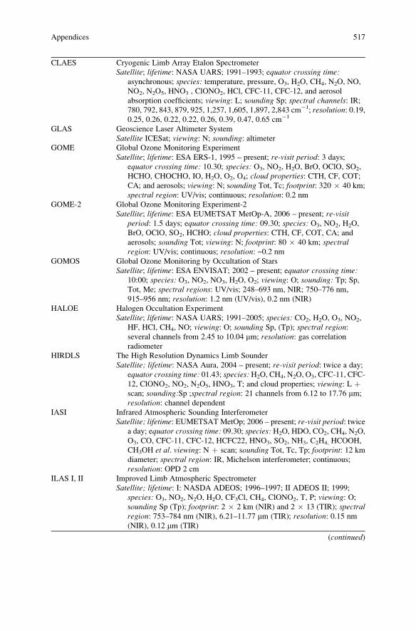
CLAES Cryogenic Limb Array Etalon Spectrometer

Satellite; lifetime: NASA UARS; 1991–1993; equator crossing time:asynchronous; species: temperature, pressure, O3, H2O, CH4, N2O, NO,

NO2, N2O5, HNO3 , ClONO2, HCl, CFC-11, CFC-12, and aerosol

absorption coefficients; viewing: L; sounding Sp; spectral channels: IR;780, 792, 843, 879, 925, 1,257, 1,605, 1,897, 2,843 cm�1; resolution: 0.19,0.25, 0.26, 0.22, 0.22, 0.26, 0.39, 0.47, 0.65 cm�1

GLAS Geoscience Laser Altimeter System

Satellite ICESat; viewing: N; sounding: altimeter

GOME Global Ozone Monitoring Experiment

Satellite; lifetime: ESA ERS-1, 1995 – present; re-visit period: 3 days;

equator crossing time: 10.30; species: O3, NO2, H2O, BrO, OClO, SO2,

HCHO, CHOCHO, IO, H2O, O2, O4; cloud properties: CTH, CF, COT;CA; and aerosols; viewing: N; sounding Tot, Tc; footprint: 320 � 40 km;

spectral region: UV/vis; continuous; resolution: 0.2 nm

GOME-2 Global Ozone Monitoring Experiment-2

Satellite; lifetime: ESA EUMETSAT MetOp-A, 2006 – present; re-visitperiod: 1.5 days; equator crossing time: 09.30; species: O3, NO2, H2O,

BrO, OClO, SO2, HCHO; cloud properties: CTH, CF, COT, CA; andaerosols; sounding Tot; viewing: N; footprint: 80 � 40 km; spectralregion: UV/vis; continuous; resolution: ~0.2 nm

GOMOS Global Ozone Monitoring by Occultation of Stars

Satellite; lifetime: ESA ENVISAT; 2002 – present; equator crossing time:10:00; species: O3, NO2, NO3, H2O, O2; viewing: O; sounding: Tp; Sp,Tot, Me; spectral regions: UV/vis; 248–693 nm, NIR; 750–776 nm,

915–956 nm; resolution: 1.2 nm (UV/vis), 0.2 nm (NIR)

HALOE Halogen Occultation Experiment

Satellite; lifetime: NASA UARS; 1991–2005; species: CO2, H2O, O3, NO2,

HF, HCl, CH4, NO; viewing: O; sounding Sp, (Tp); spectral region:several channels from 2.45 to 10.04 mm; resolution: gas correlationradiometer

HIRDLS The High Resolution Dynamics Limb Sounder

Satellite; lifetime: NASA Aura, 2004 – present; re-visit period: twice a day;equator crossing time: 01.43; species: H2O, CH4, N2O, O3, CFC-11, CFC-

12, ClONO2, NO2, N2O5, HNO3, T; and cloud properties; viewing: L þscan; sounding:Sp ;spectral region: 21 channels from 6.12 to 17.76 mm;

resolution: channel dependentIASI Infrared Atmospheric Sounding Interferometer

Satellite; lifetime: EUMETSAT MetOp; 2006 – present; re-visit period: twicea day; equator crossing time: 09.30; species: H2O, HDO, CO2, CH4, N2O,

O3, CO, CFC-11, CFC-12, HCFC22, HNO3, SO2, NH3, C2H4, HCOOH,

CH3OH et al. viewing: N þ scan; sounding Tot, Tc, Tp; footprint: 12 km

diameter; spectral region: IR, Michelson interferometer; continuous;

resolution: OPD 2 cm

ILAS I, II Improved Limb Atmospheric Spectrometer

Satellite; lifetime: I: NASDA ADEOS; 1996–1997; II ADEOS II; 1999;

species: O3, NO2, N2O, H2O, CF3Cl, CH4, ClONO2, T, P; viewing: O;sounding Sp (Tp); footprint: 2 � 2 km (NIR) and 2 � 13 (TIR); spectralregion: 753–784 nm (NIR), 6.21–11.77 mm (TIR); resolution: 0.15 nm

(NIR), 0.12 mm (TIR)

(continued)

Appendices 517

IMG Atmospheric Infrared Sounder

Satellite; lifetime: NASDA ADEOS, 1996–1997; re-visit period: 10 days;

equator crossing time: 10.30 descending; species: H2O, CO2, CH4, O3,

CO; viewing: N; sounding Tot, Tc, Tp; footprint: 8 � 8 km;

spectral region: IR; continuous; resolution: OPD ¼ 10 cm

ISAMS Improved Stratospheric and Mesospheric Sounder

Satellite; lifetime: NASA UARS; 1991–1992; species: CO2, H2O, CO, N2O,

CH4, NO, NO2, N2O5, HNO3, O3; viewing: L þ scan ; sounding Sp, Mp;

footprint: 2.6 � 13 km; spectral region: 605–2,257 cm�1 (14 Bands);

resolution: gas correlationLIMS Limb Infrared Monitor of the Stratosphere

Satellite; lifetime: NASA Nimbus 7; 1978–1979; species: CO2, HNO3, O3,

H2O, NO2; viewing: L þ scan; sounding Sp; spectral regions:637–673, 579–755, 844–917, 926–114, 1,237–1,560,

1,560–1,630 cm�1

LITE Lidar In-space Technology Experiment

Satellite Space Shuttle Discovery; lifetime: 9 days; species: aerosols, clouds;viewing: N; sounding Tot, Np; footprint: 300 m; spectral region: 355 nm,

532 nm, 1,064 nm

LRIR Limb Radiance Inversion Radiometer

Satellite; lifetime: NASA Nimbus 7; equator crossing time: local noon;species: CO2, O3; viewing: L; sounding Sp; spectral regions: IR;14.6–15.9 mm, 14.2–17.3 mm, 8.8–10.1 mm, 20–25 mm

MAPS Measurement of Air Pollution from Satellites

Satellite; lifetime: NASA Space Shuttle; 1981, 1984, 1994; species: CO;viewing: N; sounding Tc; spectral method: Gas Correlation (uses CO and

N2O as reference)

MAS Millimeter Wave Atmospheric Sounder

Satellite; lifetime: Shuttle ATLAS 1, 2 and 3:1992, 1993, 1994; species: ClO,O3, H2O; viewing: L þ scan; sounding Sp; spectral bands: 60 GHz,

183 GHz, 184 GHz, 204 GHz

MERIS Medium Resolution Imaging Spectrometer for Passive Atmospheric Sounding

Satellite; lifetime: ESA-ENVISAT; 2002 – present; re-visit period:1–2 days;

equator crossing time: 10.00 ascending; species: H2O; aerosol properties:AOD, AE; cloud properties: CA, COT, CTH, CTP; viewing: N; soundingTc; footprint: 0.3 � 0.3 km swath: 1,150 km; spectral channels: vis/NIR:412.5, 442.5, 490, 510, 560, 620, 665, 681.25, 705, 753.75, 760, 775, 865,

890, 900 nm; resolution: 1.8 nm

MIPAS Michelson Interferometer for Passive Atmospheric Sounding

Satellite; lifetime: ESA ENVISAT, 2002 – present; re-visit period: 6 days;

equator crossing time: 10.00 ascending; species: H2O, CO2, CH4, N2O,

O3, CO, CFC-11, CFC-12, ClO, ClONO2, OClO, HNO3, C2H6, SF6, NO2,

NO, NH3, OCS, SO2; viewing: L; sounding Tc (upper); spectral region:IR; FTS continuous; resolution: OPD: 20–8 cm

MLS (UARS) Microwave Limb Sounder

Satellite; lifetime: NASA UARS; 1994–2001; species: ClO, CH3CN, H2O,

HNO3, O3, SO2, temp., geopotential height, ice water content, ice water

path, relative humidity with respect to ice; viewing: L; sounding: Sp;spectral bands, 63 GHz, 183 GHz, 205 GHz

(continued)

518 Appendices

MLS (Aura) Microwave Limb Sounder

Satellite; lifetime: NASA (A-TRAIN) Aura; 2004 – present ; equator crossingtime: 13.38; species: BrO, CH3CN, ClO, CO, H2O, HCl, HCN, HNO3,

HO2, HOCl, N2O, O3, OH, SO2, temp., geopotential height, ice water

content, ice water path, relative humidity with respect to ice; viewing: L;sounding: Sp; spectral bands, 118, 190, 240, 640, 2,250 GHz

MODIS Moderate Resolution Imaging Spectroradiometer

Satellite; lifetime: Terra 1999 – present; Aqua (A TRAIN); 2002 – present; re-visit period:1–2 days; equator crossing: 10.30 descending (T); 13.30

ascending (A); aerosol properties: AOD, FM AOD, CM AOD, type, psd

(over ocean); cloud properties: CER, CIWP, COT, CPP, CTP, CTH, CTT,

LWP, DZ, CZ; viewing: N; sounding Tot; footprint: bands 1–2:0.25 � 0.25 km; bands 3–7: 0.5 � 0.5 km; bands 8–36: 1 � 1 km; swath

2,330 km; spectral channels: UV/vis/NIR; 412.5, 443, 469, 488, 531, 551,555, 645, 667, 678, 748, 858, 869.5, 905, 936, 940, 1,240, 1,375, 1,640,

2,130, 3,750, 3,859, 4,050, 4,465, 4,516, 6,715, 7,325, 8,550, 9,730,

11,030, 12,020, 13,335, 13,635, 13,935, 14,235 nm; resolution: variableMOPITT Measurement of Pollution in the Troposphere

Satellite; lifetime: NASA Terra 1999 – present; re-visit period: 3 days;

equator crossing time: 10.30 descending; species: CO; viewing:N þ scan; sounding: Tc, Tp; footprint: 22 � 22 km; spectral region: IR;correlation radiometer, 3 bands, 8 channels; resolution: 0.04 cm�1

(effective); length and pressure modulated correlation spectrometer

OMI Ozone Monitoring Instrument

Satellite; lifetime: NASA Aura (A TRAIN), 2004 – present; re-visit period: 1day; equator crossing time: 13.00 ascending; species: O3, NO2, SO2, BrO,

OClO, HCHO, CHOCHO, O4; aerosol properties: AOD, AAI, ssa; cloudproperties: CF, CP, CTH; viewing: N; sounding Tot, Tc; footprint:24 � 13 km swath: 2,600 km; spectral region: UV/vis; continuous;resolution: ~0.5 nm

OSIRIS/IRI Optical Spectrograph and Infrared Imaging System

Satellite; lifetime: Swedish ODIN, 2001 – present; equator crossing time:06.00; species: O3, BrO; viewing: L ; sounding Sp; spectral regions:280–800 nm (OSIRIS); 2 bands, 1.27 mm and 1.53 mm (IRI); resolution:1 nm (OSIRIS)

POLDER

(PARASOL)

Polarization and Anisotropy of Reflectances for Atmospheric Science coupled

with Observations from a LIDAR

Satellite; lifetime: NASA PARASOL (A TRAIN); 2004 – present; re-visitperiod: 1 day; equator crossing time: 13.30, ascending; aerosolproperties: AOD, FM AOD, CF AOD, NS AOD; cloud properties: CER,CF, COT, CP, CTH, CTP, LWP, SW albedo; viewing: N, multi-

directional; sounding: Tot; footprint: 6 � 6 km; swath: 2,400 km

spectral region: vis/NIR; polarised channels: 443, 490, 565, 670, 763,765, 865, 910, 1,020 nm

POAM-II Polar Ozone and Aerosol Measurement II

Satellite; lifetime: SPOT-3, 1993–1996; equator crossing time: 10.30descending; species: O3, H2O, NO2, aerosol properties, temperature;

viewing: O; sounding Sp; orbit: sun-synchronous polar; spectral region:UV/vis/NIR; channels, 353.0, 442.0, 448.3, 600.0, 760.8, 780.0, 920.0,935.5, 1,059.0 nm; resolution: 2–16 nm

(continued)

Appendices 519

POAM-III Polar Ozone and Aerosol Measurement III

Satellite; lifetime: SPOT-4, 1998–2005; equator crossing time: 10.30decending; species: O3, H2O, NO2, aerosol properties, temperature;

viewing: O; sounding Sp; orbit: sun-synchronous polar; spectral channels:UV/vis/NIR; 354.0, 439.6, 442.2, 603.0, 761.3, 779.0, 922.4, 935.9,

1,018.0 nm; resolution: 2–16 nm

SAGE-1 Stratospheric Aerosol and Gas Experiment I

Satellite; lifetime: NASA Atm. Explorer, 1979–1981; species: O3, NO2,

aerosol properties; viewing: O; sounding Sp, Tp (upper); spectral region:vis/NIR; channels: 380, 450, 600, 1,000 nm; resolution: 2–20 nm

SAGE-2 Stratospheric Aerosol and Gas Experiment II

Satellite; lifetime:NASA Earth Radiation Budget,1984 – present; species: O3,

NO2, H2O, aerosol properties; viewing: O; sounding Sp, Tp (upper);

spectral region: vis/NIR; channels: 385 nm, 448 nm, 453 nm, 525 nm,

600 nm, 940 nm, 1,020 nm; resolution: 2–20 nm

SAGE-3 Stratospheric Aerosol and Gas Experiment III

Satellite; lifetime: NASA Meteo 3M, 1999; ISS, 2002; species: O3, NO2,

OClO, BrO, NO3, aerosol properties; viewing: O; sounding Sp, Tp (upper);spectral channels: vis/NIR; 290, 385, 430–450, 525, 600, 740–780,920–960, 1,020, 1,500 nm; resolution: 2–20 nm

SAM II Stratospheric Aerosol Measurement II

Satellite; lifetime: Nimbus 7; 1979–1990; equator crossing time: local noon;species: aerosol properties; viewing: O; sounding Sp/Tp; footprint:30-arc-second circle; spectral region: IR; 1 channel at 1 mmwith 0.038 mmbandpass

SAMS Stratospheric and Mesospheric Sounder

Satellite; lifetime: NASA Nimbus 7; 1979–1990; equator crossing time: localnoon; species: CO2, H2O, CO, N2O, CH4, NO, temperature; viewing:L þ scan; sounding Sp, Mp (20–100 km); footprint: 10 H � 100 L km;

spectral channels: IR; 4.3, 5.3, 7.7, 15, 100 mm, 25–100 mm; resolution:gas pressure modulation technique

SBUV Solar Backscatter Ultraviolet Ozone Experiment

Satellite; lifetime: NASA Nimbus 7; 1979–1990; equator crossing time:12:00; species: O3; viewing: N; sounding: SP; footprint: 200 � 200 km;

spectral channels: UV; 252, 273, 283, 288, 292, 298, 302, 306, 312, 318,331, 340 nm; resolution: ~1 nm

SBUV-2 Solar Backscatter Ultraviolet Ozone Experiment

Satellite; lifetime: NOAA-9, NOAA- 11, NOAA-14 (1985 – present); equatorcrossing time: variable due to the satellite drift; species: O3; viewing: N;sounding: SP; footprint: 200 � 200 km; spectral region: UV; channels:252, 273, 283, 288, 292, 298, 302, 306, 312, 318, 331, 340 nm; resolution:~1 nm

SCIAMACHY Scanning Imaging Absorption Spectrometer for Atmospheric Cartography

Satellite; lifetime: ESA-ENVISAT, 2002 – present; re-visit period: 6 days;

equator crossing time: 10.00 ascending; species:O3, NO, N2O, NO2, CO,

CO, CO2, CH4, BrO, OClO, HCHO, SO2, CHOCHO, IO, H2O, O2, O4, and

aerosols ; cloud properties: CTH, COT, LWP, DZ, CZ; viewing: N, L, O;sounding Tot, Sp, Tp, Me; footprint: 60 � 30 km; spectral region:UV/vis/NIR; continuous: 240–1,750 nm, 1,940–2,040 nm,

2,265–2,380 nm; resolution: 0.2–1.5 nm

(continued)

520 Appendices

SEVIRI Spinning Enhanced Visible and InfraRed Imager

Satellite; lifetime: MSG (Meteosat 2nd Gen.); 2005 – present; geostationary,scan repeat: 15 min; species: aerosol properties: AOD, cloud properties:CTT, CTP; viewing: GEO; sounding: Tot; footprint: 1 � 1 km (high

resolution vis channel); 3 � 3 km (IR and other vis channels); spectralregion: vis/IR; channels 635, 810, 1,640, 3,920, 6,250, 7,350, 8,700,9,660, 10,800, 12,000, 13,400 nm

TANSO Thermal and short wave infra-red Sensor for observing greenhouse gases

Satellite; lifetime: JAXA GOSAT, 2009; re-visit period: 3 days; equatorcrossing time: 13.00; species: O2, CO2, CH4, H2O; cloud and aerosol

properties; viewing: N; sounding Tot; footprint: 10 � 10 km; spectralbands: vis/NIR/IR; 750–780, 1,560–1,730, 1,920–2,090,5,500–14,300 nm, resolution: 0.015–4 nm

SCR Selective Chopper Radiometer

Satellite; lifetime: NASA Nimbus 4,5; 1970–1975; species: CO2 temperature

profile, water vapour, ice; viewing: nadir; sounding Tot ; footprint:25 � 25 km; spectral region: IR(1) 4 CO2 channels between 13.8 and

14.8 mm, (2) four channels at 15.0 mm, (3) an IR window channel at

11.1 mm, H2O at 18.6 mm, two channels at 49.5 and 133.3 mm, and (4) four

channels at 2.08, 2.59, 2.65,and 3.5 mmSeaWiFS Sea-viewing Wide Field-of-View Sensor

Satellite; lifetime: SeaStar, August 1997 – present; re-visit period: 1 day;

equator crossing time: 12.20 descending; swath: 2,801 km; species: AOT(at 865 nm); viewing: N; footprint: 1.1 � 4.5 km; spectral channels:UV/vis; 412, 443, 490, 510, 555, 670, 765, 865 nm; bandwidths (FWHM):20, 20, 20, 20, 20, 20, 40, 40 nm; other features: hyperspectral image,

normalized water leaving radiance, attenuation coefficient, Angstrom

coefficient, photosynthetically active radiation, land reflectance

SME Solar Mesospheric Experiment(SME was a mission consisting of 5 single

instruments)

Satellite; lifetime: NASA SME: 1983; equator crossing time: 03.00–15.00Sun-synchronous orbit;

species: O3, O2(1Dg), NO2 sounding Sp, Me; spectral region: UV/vis

TES Tropospheric Emission Spectrometer

Satellite; lifetime: NASA Aura, 2003 – present; re-visit period: several days;equator crossing time: 01.45; species: H2O, CH4, N2O, O3, CO, NO, NO2,

HNO3; viewing: N, L; sounding Tot, Tc, Tp; footprint: 5 � 8 km; spectralregion: IR; FTS continuous spectrum; resolution: OPD: 8.45 cm

TOMS Total Ozone Monitoring Spectrometer

Satellite; lifetime: NASA Nimbus 7, 1979–1992; ADEOS, 1996–1997;

Meteor, 1992–1094; Earth Probe, 1996 to present; re-visit period: 1.5days; equator crossing time: 12.00; species: O3; SO2; viewing: N;sounding Tot, Tc; footprint: 50 � 50 km; spectral region: UV; channels:379.95, 359.88, 339.66, 331.06, 317.35, 312.34 nm; resolution: ~1 nm

Appendices 521

Appendix B: Atlas of Ancillary Global Data

Steffen Beirle

Max-Planck-Institut f€ur Chemie, Mainz, Germany

(a) Cloud-free composite of the Earth’s view from space

(MODIS/NASA).(b) Night-time light pollution derived from DMSP measurements.

Data processing by NOAA’s National Geophysical Data Center. DMSP datacollected by US Air Force Weather Agency.

(c) Normalized Differenced Vegetation Index for August 2007 from the NASA

instrument MODIS.

Terra/MODIS measurements; http://neo.sci.gsfc.nasa.gov/.(d) Fires (absolute fire counts on a 1� grid) 2003–2005, produced from ESA remote

sensing data.

ATSR World Fire Atlas, received from the ESA Data User Element.(e) Lightning flash climatology (flashes per km2 per year) derived from LIS/OTD.

The v1.0 gridded satellite lightning data were produced by the NASA LIS/OTDScience Team; http://ghrc.msfc.nasa.gov.

522 Appendices

http://neo.sci.gsfc.nasa.gov/

http://ghrc.msfc.nasa.gov

Appendices 523

Appendix C: Abbreviations and Acronyms

A list of chemical names and molecular formulae is given just before the firstchapter

Chapters

AAI Aerosol absorbing index Appendix D

AATSR Advanced along-track scanning radiometer 5, 6, Appendix A

ACCENT Atmospheric Composition Change/The European

Network of Excellence

5, 6, 10

ACE Aerosol characterisation experiment 4

ACE-FTS Atmospheric chemistry experiment – FTS 3, Appendix A

ADEOS Advanced earth observation satellite 3

ADV AATSR dual view algorithm 6

AEROCAN Canadian aerosol network 6

AERONET Aerosol robotic network – a ground based network 6, 7

AIRS Atmospheric infrared sounder 3, 4, Appendix A

AMAERO OMI multi-wavelength aerosol algorithm 6

AMF Air mass factor 2, 9

AMS American Meteorological Society 4

AMSR Advanced microwave scanning radiometer 4

AMSUA, B Advanced microwave sounding unit – A, B 4

AMV Atmospheric motion vectors 4

AOD Aerosol optical depth 6, 7, 9, Appendix D

AOS Acousto-optical-spectrometers 4

AOT Aerosol optical thickness 6, 7, 9, Appendix D

APS Aerosol polarimetry sensor 6

ARM Atmospheric radiation measurement site 5

AROME Application of research to operations in meso-scale 4

ARTS Atmospheric radiative transfer simulator 4

ASCAT MetOp’s advanced scatterometer 4

AT2 ACCENT-TROPOSAT-2 1

ATLAS Atmospheric laboratory for application and science 4

ATM Atmospheric transmission at microwaves 4

ATMOS Atmospheric trace molecule spectroscopy 3, Appendix A

ATSR-2 Along track scanning radiometer 6, Appendix A

AVHRR Advanced very high resolution radiometer 4, 5, 6, Appendix A

BAER Bremen aerosol retrieval algorithm 6

BB Biomass burning 8

BLUE Best linear unbiased estimate 9

BRDF Bi-directional distribution function 2

BRDF Bi-directional reflection function 6

BT Brightness temperature 5

BUV Backscatter ultraviolet ozone experiment Appendix A

CA Cloud albedo Appendix A

CALIOP Cloud-aerosol lidar with orthogonal polarization 6, Appendix A

CALIPSO Cloud-aerosol lidar and infrared pathfinder satellite

observations

4, 6

CAMA Toolkit for validation of OMI data 7

CARIBIC Civil aircraft for the regular investigation of the

atmosphere based on an instrument container

7

CCM Chemistry climate model 9

(continued)

524 Appendices

Chapters

CCN Cloud concentration nuclei 1, 6

CEOS Committee on Earth observation satellites 7, 10

CERES Cloud and Earth’s radiant energy system 4

CESAR Cabauw experimental site for atmospheric research 6

CF Cloud fraction Appendix A

CFC Chloroflurocarbon 3

CHAMP Challenging mini-satellite payload 4

CIMEL Commercial sun photometer 7

CIW Cloud ice water 4

CIWSIR Cloud ice water sub-millimeter imaging radiometer 4

CL Chemiluminescence 7

CLAES Cryogenic limb array etalon spectrometer Appendix A

CLW Cloud liquid water 4

CNES Centre National d’Etudes Spatiales 3

COSMIC Constellation observing system for meteorology

ionosphere and climate

4

CoSSIR Conical scanning submillimeter wave imaging

radiometer

4

COT Cloud optical thickness 5, Appendix A

CPR Cloud profiling radar 4

CRD Cloud radiation database 4

CRL Communications Research Laboratory, Japan 4

CRM Cloud resolving model 4

CRTM Community radiative transfer model 4

CSA Canadian Space Agency 3, 4

CSU Colorado State University 4

CT Cloud temperature Appendix A

CTH Cloud top height 5, Appendix A

CTM Chemical transport model 8, 9

CZ Crystal size Appendix A

CZCS Coastal zone colour scanner 5

DA Data assimilation 9

DDA Discrete dipole approximation 4

DIAL Differential absorption lidar 1, 7, 10

DMSP Defence meteorological satellite program 4

DOAS Differential optical absorption spectroscopy 1

DOFS Degrees of freedom for signal 3

DOIT Discrete ordinate iterative method 4

DPR Dual-frequency (Ku/Ka-band) precipitation radar 4

DSD Droplet size distribution 4

DU Dobson unit 2, 8, 9

DUE Data users element 6

DUP Data users program 6

DZ Droplet size Appendix A

EARLINET European research lidar network 6, 7

ECC Electrochemical concentration cell 7

ECMWF European Centre for Medium Range Weather

Forecasting

3, 4, 10

EGPM European GPM 4

E-GVAP EUMETNET GPS water vapour programme 4

ELDO European Launcher Development Organisation 1

(continued)

Appendices 525

Chapters

EMAC ECHAM/MESSy atmospheric chemistry model 9

ENVISAT Environmental satellite 3, 5, 6

EOS Earth observing system 6

EPS EUMETSAT’s polar system 4

ERTS-1 Earth resources technology satellite 6

ESA European Space Agency 1, 3, 4, 5, 6, 10

ESRO European Space Research Organisation 1

EUCAARI European integrated project on aerosol cloud climate

air quality interactions

6

EUMETNET The Network of European meteorological services 4

EUMETSAT European Organisation for the Exploitation of

Meteorological Satellites

1, 6, 10

EURAD European Air Pollution Dispersion model system 9

EUSAAR European supersites for atmospheric aerosol research 6

FFTS Fast Fourier transform spectrometer 4

FIRSC Far infrared sensor for cirrus 4

FMI Finnish Meteorological Institute 6

FT Fourier transform 1

FTIR Fourier transform infra red 7

FTS Fourier transform spectrometer 3, 4, 5

FWHM Full width half maximum 1, 3

GADS Global aerosol data set 6

GAW-PFR Global Atmospheric Watch – precision filter

radiometer

6

GCE Goddard cumulus ensemble 4

GCM Global climate model 8

GCM General circulation model 9

GCOS Global climate observing system

GEISA A spectroscopic database 3

GEMS Global and regional Earth-system monitoring using

satellite and in situ data

6

GEO Geostationary Orbit 1, 4, 10

GEO Group on Earth Observations

GEOS Goddard Earth observing system model 4

GEOS-Chem Goddard Earth observing system-chemistry model 9

GEOSS Global observing system of systems 1, 10

GLAS Geoscience laser altimeter system 6

GMAO Global modelling and assimilation office 6

GMES Global Monitoring of Environment and Security 1, 6, 10

GMI GPM microwave imager 4

GOMAS Geostationary observatory for microwave atmospheric

sounding

4

GOME-2 Global ozone monitoring experiment-2 Appendix A

GOMOS Global ozone monitoring by occultation of stars Appendix A

GOSAT Greenhouse gases observing satellite 5

GPM Global precipitation measurement 4

GPS Global positioning system 4

GPSRO GPS radio occultation 4

GRAS Global navigation satellite system receiver for

atmospheric sounding

4

GSFC Goddard Space Flight Center 4

(continued)

526 Appendices

Chapters

GVS Ground validation system 4

HALOE Halogen occultation experiment Appendix A

HERA Hybrid extinction algorithm 6

HIRDLS High resolution dynamics limb sounder 3, Appendix A

HIRS High-resolution infrared radiation sounder 4

HITRAN A spectroscopic database 3

HITRAN High resolution transmission model 4

HSB Humidity sensor for Brasil 4

HTAP Hemispheric transport of air pollution 1

IASI Infrared atmospheric sounding interferometer 3, Appendix A

ICESat Ice, cloud, and land elevation satellite 6

IDL Language used in the CAMA toolkit 7

IGACO Integrated Global Atmospheric Chemistry

Observations

10

IGOS Integrated Global Observing System 1, 10

IGS International GPS service 4

IGY International geophysical year 1

IIR Imaging infrared radiometer 6

ILAS I, II Improved limb atmospheric spectrometer Appendix A

ILS Instrumental line shape 3

IMG Interferometric monitor for greenhouse gases 3, AA

IPCC Inter-governmental panel on climate change 1, 10

IR Infrared 1, 7, 10

ISAMS Improved stratospheric and mesospheric sounder Appendix A

ISCCP International satellite cloud climatology project 4, 5

ISO International Organisation for Standardization 7

ISS International space station 4

ITCZ Inter tropical convergence zone 5

JAXA Japanese Aerospace Space Agency 1, 4, 5, 10

JCSDA Joint centre for satellite data assimilation 4

JEM-SMILES The Japanese experiment module superconducting

submillimeter-wave limb-emission sounder

4

JMA Japan Meteorological Agency 4

JPL Jet propulsion laboratory 3, 4

KNMI Royal Netherlands Meteorological Institute 6

LEO Low earth orbit 1, 4, 10

Lidar Light detection and ranging 1, 5, 10

LIF Laser induced fluorescence 7

LIMS Limb infrared monitor of the stratosphere 4, Appendix A

LIS Lightning imaging sensor 4, 8

LITE Lidar in space technology experiment 6

LOS Line of sight 2

LOWTRAN Low resolution transition model database 1

LRIR Limb radiance inversion radiometer 4, Appendix A

LRT Long range transport 8

LRTAP Long range transboundary air pollution 1

LT Lower troposphere 8

LTE Local thermal equilibrium 3

LUT Look-up table 5–7

LWP Liquid water path 5

(continued)

Appendices 527

Chapters

MACC Monitoring atmospheric composition and climate 6, 10

MAN Maritime aerosol network 6

MAPS Measurements of atmospheric pollution from satellites 3, Appendix A

MAS The millimeter-wave atmospheric sounder 4

MAS Microwave atmospheric sounder Appendix A

MAXDOAS Multi-axis differential optical absorption spectroscopy 7

MEGAPOLI Megacities: emissions, urban, regional and global

atmospheric pollution and climate effects, and

integrated tools for assessment and mitigation

6

MERIS Medium resolution imaging spectrometer 5, 6, Appendix A

METEOSAT Meteorological satellite 6

METOP MetOp is a series of three satellites, forming a segment

of EPS

4, 6

MHS Microwave humidity sounder 4

MIPAS Michelson interferometer for passive atmospheric

sounding

3, Appendix A

MIR Millimeter-wave imaging radiometer 4

MISR Multiangle imaging spectro-radiometer 4, 5, 6

MJO Madden-Julian oscillation 4

MLS Microwave limb sounder 4, Appendix A

MODIS Moderate-resolution imaging spectro-radiometer 4, 5, 6, Appendix A

MOPITT Measurements of pollution in the troposphere 3, Appendix A

MOZAIC Measurements of ozone and water vapour by in-

service Airbus aircraft

4, 7

MOZART Model for ozone and related chemical tracers 9

MSC Meteorological Service of Canada 4

MSG Meteosat second generation 6

MSS Multi spectral scanner 6

MSU Microwave sounding unit 4

MTPE Mission to planet Earth 4

MWHS Microwave humidity sounder 4

MWMOD Microwave model 4

MWRI Microwave radiation imager 4

MWTS Microwave-tomographic imaging 4

NADCC Network for the detection of atmospheric

composition change

7

NAO North Atlantic oscillation 8

NASA National Aeronautics and Space Administration

(USA)

1, 3–6, 10

NASDA National Space Development Agency in Japan 4

NCEP National centers for environmental prediction

(NOAA)

4

NDVI Normalised difference vegetation index 6

NEMS Nimbus-E microwave sensor 4

NESR Noise-equivalent spectral radiance 3

NEXRAD Next generation weather radar 4

NH Northern hemisphere 8, 9

NiCT National Institute of Information and

Communications Technology, Japan

4

NIR Near infrared 2, 6

NIS NEXRAD in Space 4

(continued)

528 Appendices

Chapters

NMHC Non-methane hydrocarbons 8

NMVOC Non-methane volatile organic compounds 8

NOAA National Oceanic and Atmospheric Administration

(USA)

1, 4, 5

NPOESS National Polar-orbiting Operational Environmental

Satellite System

1, 4, 10

NPP NPOESS preparatory project

NSF National Science Foundation 10

NWP Numerical weather prediction 1,4, 10

NWP-SAF NWP- Satellite Application Facility 4

OE Optimal estimation 3

OI Optimal interpolation 9

OMI Ozone monitoring instrument 6, Appendix A

OPAC Optical properties of aerosols and clouds package 6

OPD Optical path difference 3

OSE Observing system experiment 4

OSIRIS Optical spectrograph and infrared imaging system Appendix A

OSSE Observing system simulation experiments 4

PAH Polyaromatic hydrocarbons 1

PARASOL Polarization and anisotropy of reflectances for

atmospheric sciences coupled with observations

from a lidar

5, 6, Appendix A

PGR Polarisation gain ratio 6

PHOTONS European aerosol network 6, 7

PIA Path integrated attenuation 4

PM10, PM2.5 Particulate matter (diameter less than 10 mm)

(diameter less than 2.5 mm)

6

POAM-II, III Polar ozone and aerosol measurement II, III Appendix A

POLDER Polarization and directionality of the Earth’s

reflectances

5, 6

POP Persistent organic pollutants 1

PPS Precipitation processing system 4

PR Precipitation radar 4

PREMIER Process exploration through measurements of infrared

and millimeter-wave emitted radiation

4

PW Precipitable water 4

RADM Regional acid deposition model 9

RH Relative humidity 6

RMS Root mean square 7, 9

RMSD Root mean square deviation 6

RPV Raman-Pinty-Verstraete mode 6

RRS Rotational Raman scattering 1

RTE Radiative transfer equation 4

RTM Radiation transfer modelling 2

RTM Radiation transfer model 6, 7

RTTOV Radiative transfer for TOVS 4

RVRS Rotational-vibrational Raman scattering 1

SACURA Semi-analytical cloud retrieval algorithm 5

SAGE – 1, 2, 3 Stratospheric aerosol and gas experiment 1, 2, 3 Appendix A

SAM, II Stratospheric aerosol measurement instrument, II 6, Appendix A

(continued)

Appendices 529

Chapters

SAMS Stratospheric and mesospheric sounder 4, Appendix A

SBUV, - 2 Solar backscatter ultraviolet ozone experiment, -2 Appendix A

SCA Scene classification algorithm 6

SCAMS Scanning microwave sounder 4

SCD Slant column density 2

SCIAMACHY Scanning imaging absorption spectrometer for

atmospheric cartography

5, Appendix A

SCR Selective chopper radiometer Appendix A

SD Slant delay 4

SEVIRI Spinning enhanced visible and infrared imager 6, Appendix A

SH Southern hemisphere 8, 9

SHADOZ Southern hemisphere additional ozone sondes 7

SHDOM Spherical harmonic discrete ordinate method 4

SIBYL Selective interactive boundary algorithm 6

SIRICE Submillimeter infrared radiometer ice cloud

experiment

4

SIS Superconductor-insulator-superconductor 4

SLST Sea and land surface temperature 6

SME Solar mesospheric experiment Appendix A

SMLS Scanning microwave limb sounder 4

SMR The Odin sub-millimeter radiometer 4

SOA Secondary organic aerosol 8

SOD Slant optical density 2

SRT Surface reference technique 4

SSA Single scattering albedo 6, Appendix D

SSM/T-1, -2 Special sensor microwave/temperature-1, -2 4

SSMI/S Special sensor microwave imager/sounder 4

SST Sea surface temperature 4

SSU Stratospheric sounding unit 4

STEAM-R The stratosphere troposphere exchange and climate

monitor radiometer

4

SZA Solar zenith angle 2

TANSO Thermal and short wave infra-red sensor for observing

greenhouse gases

Appendix A

TEMIS Tropospheric emission monitoring internet service 6

TEOM-FDMS Tapered element oscillating microbalance with filter

dynamics measurement system

6

TES Tropospheric emission spectrometer 3, 7, Appendix A

THV Threshold value 5

TIR Thermal infrared 5, 6, 10

TIROS Television Infrared Observation Satellite 4, 5

TM4-ECPL Chemistry transport model version 4 – Environmental

chemical processes laboratory

9

TM5 Chemistry transport model version 5 9

TMI Tropical rainfall measuring mission microwave

imager

4

TNO Netherlands Organisation for Applied Scientific

Research

6

TOA Top of atmosphere 2, 5, 6, 7

TOMS Total ozone mapping spectrometer 5, 6, Appendix A

TORA Tropospheric ozone re-analysis method 9

(continued)

530 Appendices

Chapters

TOVS TIROS operational vertical sounder 4, 5

TP Tikhonov – Phillips regularisation 3

TRMM Tropical rainfall measuring mission 4

TROPOSAT Use and usability of satellite data for tropospheric

research

1, 10

TTL Tropopause transition layer 4, 8

UAE2 United Arab Emirates Unified Aerosol Experiment 6

UARS Upper atmosphere research satellite 4

UNECE United Nations Economic Commission for Europe 1, 10

UNEP United Nations Environment Programme 1

UNFCCC United Nations Framework Convention on Climate

Change

1

UT Upper troposphere 8

UTH Upper tropospheric humidity 4

UTLS Upper troposphere/lower stratosphere 3, 9

UV Ultra-violet 6

UV/vis UV/visible 1, 2, 7

UW-NMS University of Wisconsin non-hydrostatic modelling

system

4

VCD Vertical column density 2

VFM Vertical feature mask 6

VIM International vocabulary for metrology 7

VIRS Visible and infrared scanner 4

VMR Volume mixing ratio 8

VOC Volatile organic compound 1, 8, 9

VRS Vibration rotation spectra 1

WALES Water vapour lidar experiment in space 1

WF Weighting function 2

WFC Wide field camera 6

WMO World Meteorological Organisation 1, 10

WOUDC World ozone and UV radiation data centre 7

ZTD Zenith total delay 4

Appendices 531

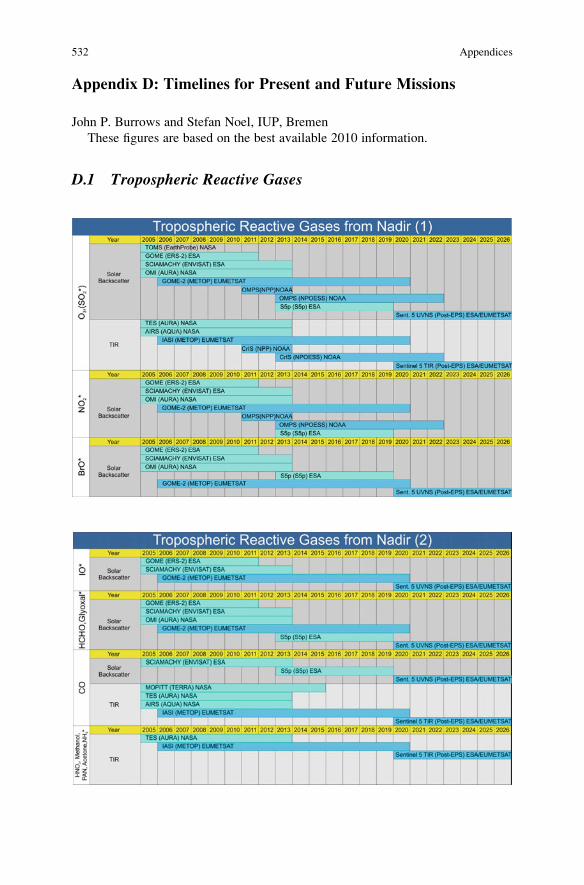
Appendix D: Timelines for Present and Future Missions

John P. Burrows and Stefan Noel, IUP, Bremen

These figures are based on the best available 2010 information.

D.1 Tropospheric Reactive Gases

532 Appendices

*Implies short lived gases with highly variable amounts. These are measured when

column amounts are above the instrumental detection limit e.g. SO2 from volcanoes

for TIR detection and from tropospheric pollution at the ground retrieved from solar

backscattered measurements

Notes

1. Concerning the retrieval of data products for tropospheric trace gases:

(a) In the TIR, the averaging kernel depends on the temperature difference

between the atmosphere and the earth’s surface. If this difference is low

Appendices 533

there is then little sensitivity to the lower troposphere and the information

content in the observation is primarily in the middle and upper troposphere.

However measurements can be made both by day and night.

(b) The retrieval of trace gases using solar backscatter is sensitive to the lower-

most troposphere as UV, visible and near IR radiation reaches the surface.

However the sensitivity is reduced in the ultraviolet as a result of multiple

scattering, and no measurements can be made at night.

2. Colouring: darker blue implies existing or funded operational meteorological

satellites and instrumentation; lighter blue implies funded space agency research

missions; the hatched pale blue implies missions under study but not yet funded.

*Used for CH4 normalisation; not optimised for CO2 retrieval

D.2 Greenhouse Gases: CH4, CO2

534 Appendices

Notes



between the atmosphere and the Earth’s surface. If this difference is low



However measurements can be made both day and night.

(b) The retrieval of trace gases using solar backscatter is sensitive to the

lowermost troposphere as UV, visible and near IR radiation reaches the

surface. However the sensitivity is reduced in the ultraviolet as a result of

multiple scattering, and no measurements can be made at night.




D.3 Greenhouse Gases: Water Vapour

Appendices 535

Notes

1. GPS refers to all Global Positioning System satellites, which are used for H2O

retrieval. These includes those already delivering water vapour products, e.g.

GRAS on METOP and COSMIC, a constellation flown by the South Korean

Space Agency in collaboration with NCAR. Further missions which are

expected to deliver water vapour products are GALILEO, GLONASS and RO

on PostEPS.



between the atmosphere and the earth’s surface. If this difference is low



However measurements can be made both day and night.

(b) The retrieval of trace gases using solar backscatter is sensitive to the

lowermost troposphere as UV, visible and near IR radiation reaches the

surface. However the sensitivity is reduced in the ultraviolet as a result of

multiple scattering, and no measurements can be made at night.




*Intermittent operation

D.4 Tropospheric Aerosol

536 Appendices

Notes

1. The aerosol optical proprieties in the figure description refer to the broad range

of aerosol data products generated. These include: aerosol optical thickness,

AOT, or aerosol optical depth, AOD, single scattering albedo, SSA, aerosol

absorbing index, AAI, size distribution where available, size discrimination,

coarse and fine.




*Intermittent operation

D.5 Clouds

Appendices 537

Notes

1. Instruments/missions often deliver different cloud products; see the individual

missions for details.




538 Appendices

Index

A list of satellite instruments is given in Appendix A.A full list of abbreviations and acronyms is given in Appendix C.A list of chemical names and molecular formulae is givenon page xxxi.

A

AATSR

aerosol retrieval algorithm, 263–266

cloud brightness measurements, 235

data products, 264, 279

retrieval of aerosol properties, 269, 279–282

Absorption linewidth, 36–37

Absorption of radiation, 26, 29, 40, 42, 51

ACCENT, 10

ACE, CO seasonal measurements, 136–138

ACE-FTS, mission example, 135–137

Acetone (CH3COCH3), tropospheric studies, 391

Acetylene (C2H2), tropospheric studies, 391

Acid deposition, 19, 21–22

Acid rain, 21

Active microwave techniques,

introduction, 195

Active systems perspectives, 507

ADEOS, 9

Aerosol

air quality role, 261

climate role, 261

data assimilation example, 478–480

model comparison, 455, 460–467

optical parameters, 266–269

over land

MODIS, 284

POLDER, 278–279

retrieval, flow chart, 286

over ocean

MODIS, 283–284

POLDER, 277–278

retrieval, flow chart, 285

scattering from, 42, 48

validation needs, 343–344

Aerosol-cloud interactions, use of satellites,

301–303

Aerosol direct radiative forcing

global averages, 298

global maps, 298

model comparison, 300–301

uncertainties, 299–301

Aerosol optical depth (AOD)

AATSR compared with AERONET, 282

comparison of ozone monitoring instrument

OMI and OMAERO, 303

estimated uncertainty, 344

Eyjafjallajoekull, 499

global from MODIS, 284, 287

to estimate PM2.5, 294

Aerosol parameters, 498–500

Aerosol products, intercomparison, 304

Aerosol properties

current instrumentation, 264

databases, 269–270

description, 260

from MERIS, 289–291

from OMI, 284–289

history of observations, 261

instruments for retrieval, 270–271

lidar, impact of, 262

multi-wavelength algorithm, 287–288

operational prediction, 417

retrieval algorithms, 262, 264–266, 270,

272, 275, 278, 280–281, 283, 305

validation, 292

Africa

biomass burning, HCHO, 378–379

CALIOP observations, 273

CH4 enhancement, 385

Air mass factor (AMF)

2-D and 3-D box, 97–98

box, 92–97

total, 91–92

539

Air pollution, 3, 11, 17–20, 25

impact, model evaluation, 455

Air quality, 2, 14, 19–20, 60

importance of NOx, 368

monitoring with satellites, 417

Airborne platforms

measurements for validation, 349

AIRS, 9, 518

CO2 transport, 142–143

Alaska, forest fires, 376, 380

Albedo

Earth’s surface, 72, 85, 89, 91, 93–94, 96,

98, 99, 105, 106, 109, 111

white & black sky, 89

Algorithm development prospects, 502–503

Ammonia. See NH3

AMSR-E, 213

AMSU-A, 167, 176, 178–181, 183–185,

206, 213

AMSU-B, 167, 173, 176, 178, 181, 184,

185, 213

Annual variability, O3, 367

Antarctica, IO measurements, 388

Anthropocene, 16, 18, 493, 512

Arctic

BrO spatial extent, 387

forest fires, 376

Asian pollution event, CO tracer, 405

AT2, 10

ATM model, brightness temperatures,

168, 169

Atmosphere

physical structure, 11–13

pressure variation with altitude, 11, 12

temperature variation with altitude, 11, 12

Atmospheric circulation, monitoring with

tracers, 404

Atmospheric composition

long term observations, 24

regional and episodic studies, 25

role of measurements, 24

Atmospheric profiles

H2O vapour, 164–166

temperature, 164–166

Atmospheric radiative transfer, 42, 46–49

Averaging kernels, derived from AMF, 95–97

B

Bayesian techniques, 161, 162, 173, 202

Beer-Lambert law, 40, 49, 73–76, 84, 92

Best Linear Unbiased Estimate (BLUE),

473–474

Biomass burning, 14, 19–21, 45,

495–497, 504

CO measurements, 371, 374, 376, 412

glyoxal observations, 379–380

HCHO detection, 378–379

NOx, 368

Bouguer-Lambert law, 40

BAER

aerosol retrieval, 289

flow chart, 285, 286

Brightness temperatures

observations, 170

simulation, 169

BrO


from volcanoes, 382, 387

global map, 399, 403

in polar regions, 387, 410

in volcanic emissions, 386

mechanism of release, 387, 410

tropospheric studies, 396

Bromine monoxide. See BrO

C

Calibration

definition, 319

CALIPSO

aerosol cloud interactions, 263, 264,

301–303, 305

aerosol retrieval, 264

cirrus cloud heights, 252

cloud retrieval, 265

instrument payload, 275

CALIOP

cloud height determination, 252

data calibration, 273–274

data products, 274–275, 277

extinction retrieval procedure,

275–276

west-central Africa, 273

Carbon dioxide. See CO2

Carbon monoxide. See COCarbonTracker system, 475

Cell correlation radiometry, 127

Central Asia, forest fires, 376

CFC, 17, 22–24, 27

fate in the troposphere, 17, 23

CFC-11, 12, 113, tropospheric studies, 398

CH4


global map, 402

inverse modelling, 471–472

regional enhancements, 385


Chemical weather, 417

Chemical weather satellites, 512

540 Index

China


CO measurements, 372, 374

NH3 concentrations, 382

NO2 monthly averages, 369

Chlorofluorocarbons. See CFCClimate change, 2, 3, 18–20, 22, 23, 47

aerosol direct radiative forcing, 297–301

operational monitoring, 416

Climate change gases, 495–496

Cloud cover, 232–234

Cloud droplets

effective radius, 232, 238–243

Cloud ice

Aura observations, 190

H2O content, definition, 168

H2O retrieval, 172–174

Cloud liquid water

definition, 168

retrieval, 170–172

Cloud parameters, 498–500, 503, 504, 507

needed accuracy for validation, 342

Cloud phase, 235–237, 246, 249, 253

Cloud products, 232, 237, 244

validation, 247–249

Cloud profiling

MODIS and CloudSat 196–197

radar (CPR), 197–198

Cloud remote sensing

hyperspectral remote sensing,

249–251

lidar remote sensing, 251–252

modern trends, 232, 249–253

Cloud screening, aerosol retrieval, 265

Cloud slicing, 102, 104

Cloud top height

CO2 slicing techniques, 245

stereoscopic method, 245

thermal IR measurements, 247

validation, 232, 249

Clouds

aerosol interactions, 263, 264,

301–303, 305

brightness temperature, 235

effect on Box AMF, 92–95

future missions, 252–253

ice path, 243–244

liquid water path, 243–244, 249, 253

microwave remote sensing, 167–170

observational history, 251

optical thickness, 231, 233, 237–240, 244,

246, 249, 250, 253

parameters, 232–247, 253, 254

reflection function, 238, 240, 241,

244, 246

CloudSat

intersection with MODIS, 199

mission, 196–197

radar, 196

CO

ACE seasonal measurements, 136–138

biomass burning, 371, 402

boundary layer residual, 415

emission estimates, 375

emissions, anthropogenic, 471–472


global emission estimates, 375

global map, 400

global measurements, 372

hemispheric transport, 374

in situ validation measurements, 317

inverse modelling, 471–472

long-range transport, 373, 374, 405

microwave observations, 191

model comparison, 471–472

model comparison for MOPITT,

464–465

model performance, 377–378

MOPITT global distribution, 141–142

SCIAMACHY/MOPITT comparison, 327,

338, 339

SCIAMACHY/OMI comparison, 337

seasonal variation, 373

transport phenomena, 373–374


upper troposphere, Aura, 191–193

validation strategy, 357

CO2

AIRS transport, 142–143


fate in the troposphere, 16

global, 384

global map, 402

ocean and atmosphere, 16–17

periodic pattern, 410

tropospheric columns, 384


Coherent radiation, 30, 44

Column density maps,

proxy for emissions, 399–404

CEOS, 494

Cryosphere, 14, 16

D

Data analysis, UV/vis/NIR

desirable improvements, 73, 75, 113

Index 541

Data assimilation

4d-var, 471–472, 474, 478–480

aerosol, 478

BLUE, 473–474

GPS results for Mediterranean, 210–211

in operational meteorology, 176–184

Kalman filter, 474

microwave radiative transfer in, 179–181

NO2 example, 474, 478

O3 example, 475

objectives & approaches, 473–475

Data centres

for validation, 354

Data comparison

data analysis, 320, 325–328

finding collocated data, 320–321

horizontal representaion, 323–324

selection and filtering, 320–322

time differences, 323

vertical representaion, 322–323

Data quality and validation. See validationDatabases, spectroscopic

HITRAN, GEISA, 126, 130

Department of Defense (DOD), 6

DIAL technique, 53, 57

Dipole moment, 32, 33

DOAS, 7, 26, 50

DOAS retrievals

advanced concepts, 83–85

considerations, 80–83

origin, 69

Ring effect, 81–82

surface reflectivity, 83

Dominant chemical pathways,

determination, 459–460

Doppler effect, thermal, 126

E

Earth observation

and remote sensing, 3–4

targets, 4

Earth shine, 72

Earth spectrum, 72

Earth’s atmosphere, thermal emission, 141

ECMWF, 502

El Nino, H2O transport, 386

Elastic scattering, 29, 43

Electromagnetic spectrum, diagram, 29

Emission of radiation, 30, 42

Emissions

CO estimates, 375

column density maps as a proxy, 399–404

constraining budgets, NO2, 369

global, CO, 375

global, NO2, 370

lightning NOx, 368, 399

NH3, 382

power plants NOx, 368

shipping NOx, 368

SO2, 380, 388, 416

soil NOx, 369, 399, 410

trends, NO2, 369

tropical, CH4, 385

Energy levels, rotational-vibrational, 125

Environmental Policy, 17–19

ENVISAT, 72, 135, 137, 139, 507

ERA-40

development, 1957 to 2002, 180

ERA-Interim

GPSRO impact, 206

ESA, 502, 507–509

Ethene (C2H4), tropospheric studies, 396

Ethane (C2H6), tropospheric studies, 396

Etna smoke plume, volcanic emissions,

49, 50

Ethyne (C2H2), tropospheric studies, 396

EUMETSAT, 502, 507–509, 512

EURAD, NO2 comparison, 477

ELDO, 6

EUMETSAT, 7, 10

ESA, 6–10, 59

ESRO, 6

EUROTRAC, 10

Eyjafjallajoekull volcano, 499

F

Fires

CO measurements, 376–377

forest, NO2 and HCHO, 370–371

NH3 emissions, 382

environmental issue, 20–21

Formaldehyde. See HCHOFormic acid (HCOOH)


Forward radiative transfer

thermal IR, 130–131

FTIR

in situ technique for validation, 357

use of data in validation, 352

Fourier transform spectroscopy

grating spectrometry, 127, 128

Frank-Condon principle, 34, 35

Fraunhofer spectrum

effect in DOAS retrievals,

80–81

Free radical reactions, 14–16

Full width at half maximum (FWHM), 37, 38

542 Index

G

GEO, 494

GEO, combination with LEO, 501

GEOS-Chem, comparison with MOPITT, 453

GEOSS, 2, 7, 694

Geostationary instruments

GeoFIS initiative, 509

GeoSCIA initiative, 509

GeoTROPE initiative, 509

GeoTropSat initiative, 508, 509

perspectives, 505–507

need for, 417

GLAS, cloud laser studies, 252

Glyoxal (CHOCHO)

annual mean concentration, 379–380


global map, 401

global mean distribution, 457–458

source apportionment, 457–459

tropospheric studies, 379–380

GMES, 7, 60

GOME, 8–10, 53, 58–60, 517

cloud top height determination,

250, 253

retrieval example, 111–113

GOME-2

effect of improved resolution, 113–115

validation activities, 354

GOSAT

FTS cloud measurements, 235

GPS

data availability, 205–207

European ground based network, 209

ground based observations, 207–209

measuring atmospheric parameters,

204–211

radio occultation, 204–205

GPSRO

impact on ERA-Interim, 206

measurement technique, 204

Greece, NH3 emissions from fires, 382

Greenhouse gases

fate in the troposphere, 17

proposed mission, 509

H

H2O

Aura observations, 192



GPS ground based observations, 207–209

hydrological parameters, 498

ice, cross sections, 159

isotope studies, 386

liquid, cross sections, 159

microwave observations, 189

refractive index for liquid and ice, 158

trends in precipitable, 386


H2O2, tropospheric studies, 397

HCFC-142b, tropospheric studies, 396

HCFC-22, tropospheric studies, 396

HCHO

annual mean concentration, 379

biomass burning, Africa, 377

column ratio with NO2, 414


global distribution, 378–379


Indian Ocean, GOME and EMAC, 456–457

proxy for isoprene, 378, 401

proxy for VOC emissions, 456–457

ship track observation, 378


HCl, tropospheric studies, 397

HCN, 376, 397, 398

HDO, tropospheric studies, 397

HIRDLS, O3 tropospheric intrusion, 140

HNO3, tropospheric studies, 397

Holocene, 493

Horizontal distribution

process impacts, 336–338

Hyper-spectral measurement perspectives, 506

I

IASI, 10, 53, 58

atmospheric radiance spectrum, 140,

144–145

SO2 global, 145

IGACO, 494, 509

global observations, 416

IGOS, 2, 494, 509, 512

India, CO measurements, 371–372

Indian Ocean

ship tracks, HCHO, 378

ship tracks, NO2, 390

Indonesia, forest fires, 376, 377

Industrial emissions, 496–497

Instrument degradation

quality assurance, 333–334

Instrument technology perspectives, 505–507

Instrumentation, idealised requirements,

504–505

Inverse modelling

CO & CH4, 471–472

future needs, 454, 472–473

principles, 454, 467–473

short-lived species, 467–470

Index 543

IO

Antarctica, 388


mechanism of formation, 388–389


UV-vis spectrum, 52–53

IPCC, 18, 19, 22

assessment, 494

IR, near. see UV/vis/NIRIR, thermal, 123–147

Isoprene, HCHO proxy, 378, 401

J

Japan, CO measurements, 372

JAXA, 7, 9

K

Korea, forest fires, 376

L

Lagrangian point satellite, 510

Lambert-Beer law, 41

Lapse rate, 11

LEO, 58–60

Lidar

differential absorption (DIAL), 53, 57

in situ technique for validation, 342–344

principle, 55, 56

Lightning, compared with NO2, 412

Limb view, 54–55, 101

Line broadening, 35–37, 125

Lorentz profile, 125–126

LOWTRAN, 45

LRTAP, 19, 20

M

Mars, atmosphere, 11

Mauna Loa observations, 24

MAXDOAS

in situ technique for validation, 350, 351

Measurement sensitivity, characterisation,

91–98

Mediterranean, HCHO tracer, 378

MERIS

aerosol products from, 304

cloud top height determination, 248

Mesosphere, 5, 11–13

Methane. See CH4

Methanol, tropospheric studies, 394

Methyl chloride, tropospheric studies, 397

MetOp satellite mission, 174, 507

Mexico City, CO measurements, 372

Microwave measurement perspectives, 506

Mie scattering, 74, 77, 79, 81, 88

polarised phase function, 44–45

MIPAS

infrared spectral coverage, 139

spectral bands, 137

Missions

need for future, 507

satellite, current and future, 507–510

MLS, 9, 187, 193, 214, 518

cloud ice and H2O vapour, 190

limb sounding observations, 191

Model evaluation

aerosol, 461

CO, 464–465

CO comparison with MOPITT, 373–374,

377–378

comparison with observation, 461–467

NO2, 462–464

use of satellite data, 463

Modelling

collocation of grid boxes and

pixels, 452

introduction, 451–454

inverse. see inverse modelling

perspectives, 481

understanding atmospheric chemistry,

455–461

Models, differences to retrievals, 460–461

MODIS

aerosol cloud interactions, 264,

301–303, 305

aerosol over the land, 284

aerosol over the ocean, 283–284

AOD-PM2.5 relationship, 296–297

cloud ice fraction, 236

cloud liquid water path, 253

cloud optical thicknesses, 238–240,

244, 253

cloud top height determination, 245, 248,

250, 253

cloud top pressure, 245, 247

cloud water droplets and ice

crystals, 242

global AOD, 287, 288, 305

monthly cloud fraction, 233, 234, 236

Molecular energy levels

rotational, 31–32

vibrational, 32–33

Molecular energy states

electronic, 34

populations, 34–35

rovibronic states, 33

Molecular spectra, 35–40

544 Index

Mongolia, NH3 emissions from fires, 382

Montreal Protocol, 18

MOPITT, 9, 53, 519

CO global distribution, 141–142

comparison with GEOS-Chem, 453

SCIAMACHY CO comparison, 327, 330,

338, 339


Multi-instrument measurements

perspectives, 506

Multi-platform observations, 414–416

Multiple observations prospects, 503

N

N2O


N2O, tropospheric studies, 393

Nadir looking instruments, 141–144

Nadir view, 8, 9, 53–54, 59, 70, 73, 75, 86,

89, 93, 94

NASA, 6–10, 23

Netherlands

AOD to estimate PM2.5, 290–293

PM2.5 map, 297

Networks

aeroplane, 346

balloon, 346

ground based, 345

ground, for validation, 331

Neural networks

Thermal IR, 133–134

UV/vis, 105

NH3, tropospheric studies, 393

Nitric acid. See HNO3

Nitrogen dioxide. See NO2

Nitrogen oxides. See NOx

Nitrous oxide. See N2O

NO2

column ratio with HCHO, 414

comparative monthly averages, 369

compared with lightning

comparison with EURAD, 477

data analysis example, 111–113

data assimilation example, 474, 478

effect of improved resolution, 112–113

emission rates, summer, 468


global emissions, 370

global map, 399–400

global transport, 370

GOME validation, 322

in situ validation measurements, 356

in situ validation techniques, 323, 324,

337, 350

MAXDOAS validation, 351, 356

model comparison, 462

model comparison for GOME, 462–463

model comparison for SCIAMACHY, 464

monthly averages, 326

monthly maximum, 410

North Atlantic transport, 370, 406

NO2, multiple roles, 496

retrieval example, 111–113

role in O3 budgets, 370

SCIAMACHY/OMI comparison, 329, 337

trends, 369, 408

Tri-cities column density, 326


validation strategy, 355–356

weekly cycle, 368, 410–411

NOAA, 6, 8, 50

North America, CO2 observations, 384

North Atlantic, transport of NO2, 370, 406

NOx

air quality, 368

biomass burning, 368, 399, 412

emissions, 368–369, 408

sources and sinks, 368

NPOESS, 507, 512

NWP, 508, 509, 512, 513

O

O2 A-band spectrometry

cloud height determination, 248

cloud top height, 248

O2, UV spectra, 13

O3

annual variability, 367

budget, role of NO2, 370

Chappuis Bands, 104

data assimilation example, 475–476


global distribution, 367

global map, 400

Hartley Bands, 68, 83

highlights, 495

Huggins Bands, 70

in situ validation measurements, 346–348

ozone assessments, 18

ozone hole, 17, 23, 25, 70

production and loss, 13

stratospheric depletion, 19, 22–23

tropical Atlantic, TES, 143–144

tropical columns, 367

Index 545

O3 (cont.)tropospheric, 366–368, 378, 401, 403,

406, 408, 412

tropospheric and air quality, 19–20

tropospheric intrusion, HIRDLS, 140


validation strategy, 355

Observation techniques, in-situ, 25–26Occultation, 8, 10, 55, 71, 73, 86

Occultation instruments, limb and solar,

135–140

OCS, tropospheric studies, 396

OH, a free radical, 14

OMAERUV

data product from OMI, 285, 303

data product status, 288–289

OMI, 9, 53, 58, 519

aerosol cloud interactions, 264

aerosol products from, 270, 284–287

data assimilation of NO2, 477

effect of improved resolution, 113

SCIAMACHY CO comparison, 339


Operational use of satellite instruments,

416–417

Operator dilemma, 24

Optimal estimation (OE) formalism,

131–133

Orbits

GEO, 60

LEO, 58–60

polar, 57–59

satellite, 57–58, 60

sun-synchronous polar, 58, 59

Ozone. See O3

P

PAN, 16


PARASOL


Particle scattering, 74, 88

Peroxy nitric acid, tropospheric

studies, 397

Persistent organic pollutants (POPs), 18, 19, 21

Photochemistry, fast in-situ investigation, 25

Planck’s law, 123–126

PM10, data assimilation with SYNAER,

479–480

PM2.5, AOD estimate in the Netherlands,

292–293

Polarisation measurement perspectives,

505–506

POLDER

aerosol over land, 278–279

aerosol over the ocean, 277–278

Population, growth of human, 18

Profiles, synergistic approaches, 413–414

Q

Quality assurance

algorithm optimisation, 333

calibration, 331–332

instrument degradation, 333–334

lower level products, 332–333

quality monitoring, 334–335

validation and mission planning, 331

R

Radiation, interaction with matter, 28, 30,

40, 44

Radiative transfer modelling

input data, 98–99

molecular absorption processes, 90

molecular scattering, 86–88

overview of models, 99–101

surface reflection and absorption, 89

to interpret observations, 86–90

Raman scattering, 30–31, 44

Rayleigh scattering, 29, 30, 43–46, 48, 74, 81,

82, 86–88, 90, 91, 93, 105

Reflectivity, ground cover and river water,

50, 51

Refractive index, complex, definition, 260

Remote sensing

active techniques, 55–57

and Earth observation, 3–5

back scattered solar radiation, 5, 7–9

definition, 1

from space, 1–60

historical milestones, 6–7

images and spectroscopy, 49–57

limb view, 54–55

nadir view, 53

nadir, limb and occultation, 53–55

occultation, 55

of the troposphere from space, 2, 8

passive and active, 4, 31, 53, 54

passive techniques, 4, 7

perspectives, 505–507

scientific highlights, 495

scientific needs, 500–501

techniques, versus in situ, 26–27thermal IR, 9–10

validation observations from the ground,

349–353

546 Index

Retrieval of satellite data, desirable

improvements, 113–114, 412

discrete wavelength techniques, 76–78

examples, 111–113

separating different effects, 76–77

separation of stratopheric signal, 101–102

synergistic approaches, 412

differences to models, 460–461

Russian forest, fires, 370

S

SAGE, 8

Satellite instruments, desirable developments,

113–114

Satellite instruments, synopsis, 110–111

Satellite observations, needs, 493–495

applications, 365–418

what can we learn?, 399–417

examples, 111–113

histroy, 110–111

synergistic use of complementary, 115

viewing geometries, 70–73

Satellite orbits, 57–60

SBUV, 7, 8, 23, 53, 70, 71, 102, 110, 520

Scattering, atmospheric, 42–49

elastic, 29, 30, 43

inelastic, 31, 44

SCIAMACHY, 8, 10, 53, 55,

58, 60, 72, 73, 78, 80, 103, 106,

110, 111, 115, 520

cloud phase index measurements, 235

cloud top height determination, 248

data assimilation of NO2, 478

MOPITT CO comparison, 327, 330,

338, 339

OMI CO comparison, 339


Scientific highlights, 495

Scientific needs, 500–501

SE Asia

forest fires, 376

HCHO detection, 378

SEVIRI


SF6, tropospheric studies, 398

Ship tracks

HCHO, Indian Ocean, 378

NO2, Indian Ocean, 370

Siberia

NH3 emissions from fires, 382

NO2 and HCHO from fires, 370–371

Slant column density, 73, 75, 77, 84, 91, 93,

101, 106, 111, 113

Smog

photochemical, 16–18

summer (See Smog, photochemical)

winter, 17SO2


from Soufriere Hills volcano, 399, 404,

405, 416

global map, 399

IASI global, 145

industrial emissions, 380–382

long-range transport, 382

tropospheric studies, 380–382

volcanic emissions, 381

SOA, role of glyoxal, 379

Solar spectrum, GOME, 72

Source identification, synergistic approaches,

412–413

South America


SO2 from volcanoes and smelters, 404

Space agencies

Canadian, 7

Chinese, 7

European (ESA), 6, 7

Indian, 7

Japanese (JAXA), 7

Korean, 7

United States (NASA), 6

USA, 6, 7

Spectral line broadening mechanism, 39

Spectral line shape

Doppler, 35, 37–38, 40

in different ranges, 39

Lorentzian, 37, 39

Spectral linewidth

doppler broadening, 37–40, 52

natural, 37

pressure broadening, 37–39, 52

Spectral retrieval, DOAS type, 78–80

Spectroscopic techniques

IR, 52

microwave, 51–52

UV/vis/IR, 52–53

for chemical analysis, 40–42

Spectroscopy

absorption, 40–42

emission, 42

Stefan-Boltzmann law, 124

Stimulated emission of radiation, 30

Stratosphere, 4, 8, 11–13, 15–17, 20, 23, 24, 52

Stratospheric signal separation

cloud slicing, 104

Index 547

Stratospheric signal separation (cont.)model method, 103–104

other approaches, 104–105

residual measurements, 103

stratospheric measurements, 102–103

Stratospheric variability

causes, 338–340

Sulfur budget, 380

Sulfur dioxide. See SO2

Summer smog. See Smog, photochemical

Sun glint, 89, 90

Sun photometers

in situ instrument for validation, 353

Sun synchronous polar orbit, 58, 59

Surface reflection

Surface reflection and absorption

albedo, 89

ocean surface interactions, 89–90

Surface reflection, angular dependency,

89–90

SYNAER, data assimilation for PM10,

479–480

Synergistic use of satellites, 367, 413, 415

T

TES, 10, 53, 58, 521

data comparison, 322

O3 tropical Atlantic, 143–144


Thermal IR

absorbing molecules, 135, 136

future plans, 145–147

history, 145–147

instruments and techniques, 127–128

physical principles, 123–127

products, 135–140

specificity, 129–134

Thermosphere, 5, 11–13

Tikhonov-Philips regularization, 133

Tomographic reconstruction perspectives, 506

TOMS, 8, 23, 53, 70, 71, 77, 78, 102, 110, 521

Trace species, others measured from space, 366

Transitions, allowed and forbidden, 34, 35

Transpacific Asian pollution, comparing

MOPITT with GEOS, 453–454Transport

CO, 376

global, NO2, 370

hemispheric, CO, 370, 374–376

monitoring with tracers, 404

Trends

CO2, 409

NO2, 369, 408, 417

Tropical rain forest, CH4 deviations, 385

TROPOSAT, 10

Troposphere

acid deposition, 19

and climate change, 19, 22, 23

biomass burning, 14, 19

chemistry, 11–23, 60

complex chemical interactions, 15, 16

composition, measurement need

environmental issues, 19

impact of stratospheric O3 depletion,

22–23

O3 and air quality, 19–20

POPs, 21

Tropospheric chemistry, 11–23, 60

Tropospheric composition

applications of satellite observations,

365–418

synergistic approaches, 416

Tropospheric compounds, observed,

495–496

Tropospheric intrusion of O3, 140

Tropospheric photochemistry

role of halogen chemistry, 386

Tropospheric trace gases

measured from space, 392

U

Uncertainties in satellite measurements

instrument noise and stray light, 106–107

instrument slit width, 107

light path, 108–109

spectral interference, 107–108

spectroscopic uncertainties, 107

tropospheric/stratospheric separation,

109–110

UNECE assessment, 494

UNFCCC, 18, 22

United Arab Emirates, AOD over, 282

USA, forest fires, 376

UV/vis/NIR

future developments, 113–115

historical background, 67–69

satellite observations, 70–73

species retrieved, 73–76

uncertainties in measurements, 105–110

V

Validation

aerosol effects, 341–343

albedo effects, 341–343

characteristics of tropospheric products,

335–336

cloud effects, 341–343

548 Index

comparing data sets, 320–328

data treatment, 322–325

data variability, 329–330

definitions, 319–320

future strategies, 354–357

introduction, 315–318

methods, 348

stratospheric gas effects, 338–341

use of models, 328–329

Venus, atmosphere, 11

Vertical column density, 68, 75, 93, 97,

106, 113

Vertical distributions of trace gases

determinants, 336

process impacts, 336–337

Vienna Convention, 18

Voigt profile, 126

Volcanic emissions

particulate matter, 500

SO2, 500

W

Wavenumber, definition, 28

Whiskbroom scanning scheme, 59, 60, 110

Wien’s law, 124

WMO assessment, 494

Index 549

appendices - rd.springer.com978-3-642-14791-3/1.pdf · tc tropospheric column, sc stratospheric...

Documents