appendices for the paper: design and analysis of a high...

Lange, Relativity Gyroscope

1

Appendices for the Paper: Design and Analysis of a High-Accuracy Version

of the Relativity-Gyro Experiment. Deposited in the PHYSICS

AUXILIARY PUBLICATION SERVICE for PRD15.

Benjamin Lange1922 Page Street, San Francisco, CA, 94117-1804

Fax: (415) 221-5335, email: [email protected]

Appendix A. Calculations of the Major Gyro Drifts ................................................................................................... 1Appendix A1. The Physical Basis of the Gravity-Gradient Drift ......................................................... 2Appendix A2. The Gravity-Gradient-Drift Errors.......................................................................................... 2Appendix A3. Magnetic-Eddy-Current, Barnett-Effect, and Spinning-Charge Drifts................. 5Appendix A4. Roll Averaging............................................................................................................................. 6Appendix A5. Gas Brownian Motion and Gas Spin-Down Drifts ....................................................... 7Appendix A6. Rotor Collisions with Large Particles in the Cavity .................................................. 8Appendix A7. Flat Differential Pressure........................................................................................................ 8Appendix A8. Electric Fields in the Cavity................................................................................................. 8

Appendix B. Zero-Gravity-Gradient Orbits...................................................................................................................... 9Appendix C. Autocollimator Performance........................................................................................................................ 10

Appendix C1. Autocollimator Noise Equivalent Angle............................................................................ 11Appendix C2. Autocollimator Zero-Point Errors.......................................................................................... 12Appendix C3. Autocollimator Scale-Factor Errors..................................................................................... 13Appendix C4. Transcollimator.............................................................................................................................. 14

Appendix D. Summary of the Technique for Placing the Optical Flats on the Rotor................................ 14Appendix E. Telescope Performance .................................................................................................................................. 16

Appendix E1 Telescope Noise Equivalent Angle....................................................................................... 16Appendix E2. Telescope Zero-Point Errors..................................................................................................... 17Appendix E3. Telescope Scale-Factor Errors................................................................................................ 18

Appendix F. Roll-Coupled Zero-Point Errors and Drifts............................................................................................. 22Appendix G. Instrument Scale-Factor Calibration Accuracy.................................................................................. 25Appendix H. Operational and Miscellaneous Considerations................................................................................. 27

Appendix H1. Entering the Counter-Rotating Orbits.................................................................................. 27Appendix H2. Radiation Environment .............................................................................................................. 27Appendix H3. Active Damping............................................................................................................................ 28Appendix H4. Absolute Temperature Control ............................................................................................... 28Appendix H5. Planetary Structure of the Reference Star........................................................................ 28Appendix H6. Testing............................................................................................................................................... 28Appendix H7. Four Gyros Versus One.............................................................................................................. 28

References....................................................................................................................................................................................... 29Detailed Acknowledgments..................................................................................................................................................... 30

Appendix A. Calculations of the Major Gyro Drifts

This appendix will emphasize the largestsources of gyro drift as well as those which were nottested by the 1972 drag-free flight [39]. These includegravity gradient, magnetic, gas brownian motion, large-particle, and spurious electric-field drifts. The balanceof the drifts can be calculated from the expressions inTable 2 or can be found in References 2 or 32. Thecoordinate system used in the appendices is the gyro-

frame with the z-axis parallel to the gyro angularmomentum axis and the x-axis as close to the earth'sspin axis at J2000.0 as possible. With this definition,the axis which measures the geodetic drift is rotationabout the y-axis (the experiment axis); and rotationabout the x-axis is the cross axis, i.e. the axis used tomeasure the gyro performance and/or the frame-draggingdrift.


2

Appendix A1. The Physical Basis of the Gravity-Gradient Drift

The first question which should arise in adesign with an autocollimator readout is will the opticalflats cause unacceptable gyro drift by making thesurface nonspherical and by unbalancing the principalmoments of inertia? It can been seen from the table ofgyro drifts that the effect of the flats on drifts fromtorques due to surface forces is negligible. The gravity-gradient drift, however, is directly proportional to themoment-of-inertia difference ratio, ∆I / I = εT , i.e. εTotal .εT arises from two sources, a permanent ∆I / I = εp andan elastic ∆ I / I = ε elastic caused by the rotor spin.εp comes from the slightly nonspherical surface, densityinhomogeneities, and the optical flats which are itsprimary cause. When two optical flats are ground ontothe north and south poles of the rotor, the resultingpermanent ∆I / I is given by εp =15(df / dr)

4/16 where df

is he diameter of the flat and dr is the rotor diameter.Thus two optical flats 5 mm in diameter on a 5-cmdiameter rotor give εp ≈ 10-4. This is about 100 times aslarge as the value of ∆I / I caused by the polishing errorsand density inhomogeneities.

For a rotor constructed from a homogeneous,isotropic elastic material spinning at rate, ωG , the un-compensated gravity-gradient drift averaged around a

circular orbit, φav , is given by [47, 32, 2]

˙ ( )

.

φω

ε θω

ε ε θ

εω

ρ ω θν

avG

T mlG

p elastic ml

p

GG ml

n n

nk a

E

= = +

= +

32

32

32

2 2

22

A1

θml is the effective misalignment between the spin axisand the orbit plane or the orbit normal depending on theexperiment, ρ = 2340 kg/m3 for Silicon, a = 2.5 cm, andE is the Young's modulus of Silicon = 1.7×1011 N/m2.εelastic = kνρ a2ωG

2 / E where kν = (ν + 1)(ν + 2) / (5 ν + 7)

and ν is Poisson's ratio = 0.22 for Silicon givingkν = 0.33.

Equation A1 has an optimum value of ωG whichminimizes the drift rate with εp equal to εelastic,

ωερν

G optpE

k a= 2 . A2

This value of ωG gives a minimum gravity-gradient driftrate of

˙minφ

ρ εθν

avp

mln ak

E= 3 2 . A3

Equation A2 gives a rotor spin rate of 924 Hz for a 2.5-cm radius Silicon rotor with εp = 10-4; and once the rotorsize and material have been chosen, the gravity-gradient drift is determined only by the effective valueof θml and the square root of εp.

Based on Equation A3, it might be thought thatthe correct approach to reduce the gravity-gradient driftwould be to make εp as small as possible. This is,however, undesirable as the optimum spin speed is alsoproportional to the square root of εp, so that a small εp

results in a low rotor speed which increases the driftsfrom other torque sources such as gas brownian motion.Furthermore, a smaller εp only improves the drifts asεp

1/2 so that making it smaller than 10-4 does not bring asignificant gain over the best spheres which can be pol-ished (εp = 10-6), only a factor of 1001/2 = 10. In addi-tion, reducing the gravity-gradient drift by making εp

very small is also undesirable because it makes therotor harder to manufacture and makes the measurementof the flat alignment more difficult. On the other hand,the effective value of θml may be made so small by theproper choice of the orbit that εp = 10-4 gives acceptablegravity-gradient drifts. These considerations are impor-tant since they show that it is not desirable to attempt tofabricate a gyro rotor of any better quality than εp = 10-4

which is the natural value that arises with two flats tenpercent of the diameter of the rotor.

Appendix A2. The Gravity-Gradient-Drift Errors

The simulation in Appendix B shows that theorbit can always be chosen to return the y-gravity-gradient-drift angle (the experiment axis) to zero at theend of the year, but a perfect orbit cannot be obtained inpractice. The question then arises what is thesensitivity of the y-gravity-gradient drift to the orbiterrors, and how large are these errors. In calculatingthese sensitivities, one can also consider thex-component of the geodetic drift; since it also dependson the orientation of the orbit plane.

For the geodetic experiment where the gyrospin vector is in the orbit plane, there are only fournonzero first-order sensitivity terms. They may be cal-culated to a few percent accuracy from the naïve formu-las for the drifts due to orbit misalignment without tak-ing account of all of the external disturbances from the


3

sun, moon, precession, nutation, the earth's real gravityfield, etc. since they come from a trajectory linearizedwith respect to the more exact orbit. If i' is the coincli-nation (90º - i), Ω is the right ascension relative to thereference star, φy is the y-component of gravity-gradientdrift, and gx is the x-component of the geodetic drift; thefour non-zero sensitivities for the positive orbit are givenby:

∂ φ∂

φ δ φ ∂∂

δygg ggi

ti

t

0 0

2

2'˙ sin ˙

˙

'cos= − − Ω

, A4

∂ φ∂

φ δyggtΩ0

= − ˙ cos , A5

∂∂

δ ∂∂

δg

ig t g

i

txgeo geo

0 0

2

2'˙ cos ˙

˙

'sin= − Ω

, A6

and

∂∂

δgg tx

geoΩ0

= − ˙ sin A7

where δ is the declination of the reference star,˙ /φ ε ωgg T Gn≡ 3 22 , and ˙ /g GM n c rgeo s≡ ⊕3 2 2 . Table A1

shows the theoretical sensitivities with respect to theinitial coinclination and relative longitude of theascending node calculated from the above expressionsfor a one-year experiment as well as the averagex-gravity-gradient drift angle which will be discussed be-low.

Table A1 shows that only ∂ φy / ∂ i 0 ' (orequivalently during the year, ∂ φy / ∂ i') is important; andthe calculations for the compensation errors will bebased only on this term. Since the orbits are chosen todrive the final value of the gravity-gradient drift to zeroin the experiment axis and the final value of the geode-tic drift to zero in the cross axis, it is the sensitivitieswhich determine the y-gravity-gradient and x-geodeticdrift errors.

Star Declination∂ φ∂

y

i0'

∂ φ∂

y

Ω0

∂∂

g

ix

0'

∂∂

gx

Ω0

φx

(deg) (µas / ") (µas / ") (µas / ") (µas / ") µas

Achernar -57.24 12.1 -0.72 -294.7 20.3 -22.2Rigel -8.204 20.2 -1.32 -28.4 3.44 -6.88Capella 46.00 13.1 -0.93 280.0 -17.3 24.3Mintaka -0.2992 20.2 -1.33 22.2 0.126 -0.25Alnilam -1.202 20.2 -1.33 16.4 0.506 -1.02Canopus -52.70 13.3 -0.81 -276.5 19.2 -23.5Sirus -16.72 19.8 -1.28 -82.2 6.9 -13.4Procyon 5.225 20.0 -1.33 57.3 -2.2 4.42Mimosa -59.69 11.4 -0.67 -303.8 20.8 -21.2Hadar -60.37 11.2 -0.66 -306.2 21.0 -20.9Arcturus 19.18 18.7 -1.26 143.0 -7.9 15.1δ Oct -83.67 3.55 -0.147 -361.1 24.0 -5.34Rigel Kent -60.84 11.0 -0.65 -307.9 21.1 -20.7Vega 38.78 14.9 -1.04 248.1 -15.1 23.8Melik -0.3197 20.2 -1.33 22.1 0.135 -0.27Polaris 89.26 -1.07 -0.0171 366.3 -24.1 0.626

Table A1. One-Year Drift-Angle Sensitivities, 1500-km Polar Orbit

The other two components, the y-geodetic driftand the x-gravity-gradient drift, have no first-order sensi-tivity to the orientation of the orbit plane. Furthermore,the y-geodetic drift is the desired outcome of the exper-iment, and for a spherical earth the average value of thex-gravity-gradient drift is zero. This average, however,

is not exactly zero due to the presence of the J2 term inthe earth's gravitational field. It is the sum of two ef-fects: a rectification of the twice per orbit altitude oscil-lations due to J2 with the twice-orbit oscillations of theinstantaneous x-gravity-gradient drift and a term stem-


4

ming directly from J2. The last column of Table A1shows its value for the stars listed there. Since it is alsodesired to simultaneously measure the frame-dragging

drift to high precision, φx is an error term for that mea-surement; and it is desirable to compensate this drift.Its value is given by

˙ sin( )φ εω

δxT

G

e

s

Jn R

r=

316

22

2 2

. A8

A twice-orb i t osc i l l a t ion of ampl i tude3 n εT / 4 ωG = 4.82 µas is superposed on the average driftangle from Equation A8. This is the term which rec-tifies with the J2-induced altitude oscillations to givepart of the expression in Equation A8.

Although the physical y-gravity-gradient driftangle at the end of the experiment is determined by thedeviation of the real orbit from the ideal orbit, this anglecan be calculated to an accuracy which depends on theaccuracy with which the orbit can be measured duringthe year. Compensation by calculation is standard prac-tice for ultra-low-drift inertial-quality gyros and will alsobe used here to gain the last factor of approximately six

in the gyro performance. Table A2 shows the errors inthis calculation and also in calculating the precisevalue of the geodetic drift. It will be assumed thatAlnilam is the reference star, that the orbit can maintaini' within about 10 mas of the ideal orbit, and that i' canbe measured to 1.5 mas which corresponds to a cross-track error of 5 cm [42]. The orbit plane errors for the y-gravity gradient can then be calculated by multiplyingthe value in Table A1 for ∂ φy / ∂ i0' by 0.0015. Thex-geodetic sensitivities to the orbit-plane errors are simi-larly calculated. The altitude errors are calculated bydifferentiating the drift with respect to the radius vectorand multiplying by 5 cm, i.e. ∂ φy / ∂ i0' × 0.01 is mul-tiplied by 3 × 5 cm / rs . The rotor-spin errors assumethat the gyro spin speed can be measured to one part in109. The compensation of ∆I / I assumes that the elasticbulge of the rotor can be calculated to 0.1 percent whichcorresponds to dividing the drift by 2000 since the per-manent bulge can be measured to very high precisionfrom the polhode period so that only half of the bulgehas the 0.1 percent error. The geocentric gravitationalconstant, G M⊕ , is assumed to be known to one part in109 [48]; and to get its error contribution, the gravity-gradient drift is multiplied by 10-9 and the geodetic driftby 1.5 × 10-9.

Error Source Experiment Cross AxisAxis (y-axis) (x-axis)

(µas/yr) (µas/yr)

Gravity Gradient Orbit Plane 0.0304Declination 1.02E-07

Altitude 3.86E-09 1.30E-08Rotor Spin 2.02E-10 1.02E-09

εp 0.0001 0.00051G M⊕ uncertainty 2.02E-10 1.02E-09

RSS 0.0304 0.00051

Geodetic Orbit Plane 0.0246Altitude 0.0790 3.13E-07

G M⊕ uncertainty 0.0075 2.46E-08

RSS 0.0790 0.0246

Table A2. Gravity-Gradient Compensation and Geodetic Drift Calculation

The compensated drifts in the cross-axis deter-mine how accurately the gyro drift performance can bemonitored during the experiment as well as the errors ina simultaneous frame-dragging measurement for which

the geodetic drift as well as the gravity gradient is anerror source. It can be seen that the principle error incompensating the gravity-gradient drift is the trackingerror.


5

Appendix A3. Magnetic-Eddy-Current, Barnett-Effect, and Spinning-Charge Drifts

Since the Unsupported Gyro is spun up,damped, and aligned with the reference star by meansof an eddy-current induction motor, the rotor must beslightly conducting. This also eliminates the problem ofcharges being trapped in the interior of the rotor. A con-ducting rotor, however, is subject to drift due to torquesfrom eddy currents induced in the rotor by the earth'smagnetic field. Thus the rotor conductivity must bechosen to provide adequate spinup torque withoutcausing excessive gyro drift. It turns out that (withproper shielding) this can be done. The expression forthe eddy-current drift given in Table 2,

/ = ⊥φσ

ρave e AC m orbitB B S C A2

4,

is derived in [32]. It depends on the components of theearth's magnetic field perpendicular and parallel to thespin axis, Be⊥ and Be , the AC attenuation at roll

frequency of the magnetic shield, SAC , and the averagingfrom the orbit, Aorbit . C M is the compensation of theeddy-current drift, if any, which might be applied.CM = 1 means no compensation; and CM = 0.1, for ex-ample, implies that a calculation with a 10 percent errorhas been used to compensate the drift. In the idealcase, the average drift would be zero [2], that is, theaverage of B Be e⊥ in a circular orbit around a rotating

inclined dipole is zero if the gyro spin axis is parallel orperpendicular to the dipole rotation axis and parallel orperpendicular to the orbit normal. This is obvious if thedipole is parallel to the earth's rotation, but it is alsotrue for an inclined dipole. The values in Table 2 werecalculated by numerical integration of the orbit usingthe IGRF model (Cf. Appendix B). Because the aver-age of the eddy-current drift is ideally zero, it is impor-tant to determine the actual drift through simulation andnot from the peak values. For example with Be = 0.3gauss and σ SAC

2 CM = 10-5 mhos/m, the formula for thepeak eddy-current drift above gives a value of 6.3 µas/yrwhich is about 900 times greater than the simulationvalue in Table 2 for Alnilam with a declination of –1.2deg and about 3500 times greater than the equatorialstars Mintaka and Saad el Melik. Because the drift isproportional to the square of the AC magnetic shieldingand the first power of σ, the simulation may be used tostudy any combination of these parameters by scalingthe results as σ SAC

2.

In addition to the gyro drift caused by eddy cur-rents in a conducting rotor, there are two other magneticdrift sources which arise because the rotor spin causes itto have a magnetic moment. One is the Barnett effectand the other is spinning charge on the rotor. Both ofthese drifts go as the first power of the shielding andeventually come to dominate the magnetic drifts as theshielding improves. The Barnett effect is due to the factthat rotating a material body causes the electron spinand orbital angular momenta to attempt to line up withthe rotation axis so that by the gyromagnetic theorem,rotor spin induces a magnetic moment, mH , in a solidbody. This moment is given by

mHol m

m eG

V

g e m= 2

0

χµ /

ω A9

where Vol the volume of the rotor, χm the magnetic sus-ceptibility, µ0 the permeability of free space, gm theg-factor for the gyromagnetic ratio of the bulk material,and e / me the electron charge to mass ratio. This mag-netic moment interacts with the ambient magnetic fieldto produce a mechanical moment which causes a gyrodrift proportional to the magnetic field.

The spinning-charge drift is caused by the factthat a spinning charged rotor generates circulating cur-rents with a magnetic moment given by

mH ol GV a d V= +( )ε0 1 / ω A10

where V is the potential due to the charge on the rotor.The factor (1 + a / d) arises because the cavity shieldwith gap, d, increases the effective capacitance of therotor. The spinning-charge drift has exactly the sameform as the Barnett drift and can be obtained by multi-plying the results of the Barnett simulations by a numer-ical factor,

˙ ( / ) ˙

. ˙

φ φ

φ

sp chgm

e mBarnett

Barnett

g eV a d

m c

V

= +

= −

1

2

0 9201

2 χ

voltA11

The requirement on any residual constant fieldinside of the magnetic shield is much less severe thanfor AC fields such as Be . This is because any constantmagnetic fields arising from the satellite are roll aver-


6

aged by the satellite's spin, and magnetic fields fromcurrents at roll frequency such as from the solar panelscan be designed to be smaller than the earth's field. Aninternal satellite-fixed field would arise becausemumetal shields also typically have a small constantresidual magnetic field inside of the shield due to mag-netization of the shield itself. It is important to estimatehow well roll averaging and the magnetic shield elimi-nate drifts caused by constant magnetic fields internalto the satellite. For this calculation, the inertially fixedcomponent of satellite attitude misalignment with re-spect to the gyro, εAtt , will be taken as 10-8 radians orabout 2 mas attitude error. (εAtt is used instead of the ef-

fective roll averaging, A, because the rotor cavity posi-tion plays no roll in this calculation since the product ofBi ∆ Bi where ∆ Bi is the change due to the field gradientis much smaller than Bi

2). Gyro drift from this sourcewould then arise because the spin down torque causedby the angular velocity of the rotating magnetic fieldseen by the rotor, which is the difference between thegyro spin rate and the satellite spin rate, is misaligneddue to this angle. For εAtt = 10-8 rad and a drift require-ment of 0.006 µas/yr, this effect sets a limit on a resid-ual field of 0.3 × 10-3 Gauss = 3 × 10-8 Tesla, i.e. about1000 times smaller than the earth's field.

7×10-3 µas/yr Conductivity, σ Shielding, SAC Compensation, σ SAC2CM

mhos/meter CM mhos/meter

Baseline 105 10-5 1 10-5

Backup 1 103 10-4 1 10-5

Backup 2 104 10-4 0.1 10-5

Table A3. Conductivity, Attenuation, Compensation Combinations

The magnetic shield is a sphere with an outerdiameter of 25 cm consisting of four or more layers ofone-mm mumetal spaced one cm apart with an initialpermeability of 120,000 and a maximum permeability of350,000. The drift specification requires that the combi-nation σ SAC

2CM be less than 10-5 mhos/meter for an eddycurrent drift of 7 × 10-3 µas/yr for Alnilam. The require-ment is expressed in this form because the exact degreeof shielding which can be obtained is controversial9 .Table A3 shows example of various combinations whichcan fulfill the drift requirements.

Appendix A4. Roll Averaging

The gyro drifts can be greatly reduced by rollaveraging the satellite-fixed disturbing torques. The pre-cision with which roll averaging can be maintained de-pends on the accuracy with which the drag-free controlsystem can keep the rotor inertially centered in the cav-ity, the accuracy with which the satellite attitude con-

9 Two shield manufacturers, Vacuumschmeltze andMu Shields, claim that they can furnish flightqualified multilayer shields with an AC attenuation of3 × 10-6 or even 10-7, but two GPB team memberswith considerable experience in magnetic shieldingclaim that reliable attenuation better than 10-4 is notpossible.

trol system can hold the inertial component of the spinaxis of the satellite aligned with the spin axis of thegyro, and the number of roll cycles.

These accuracies depend on the noise in thepickup systems, the disturbing forces and torques, thealignment of the center of mass of the satellite with thecenter of the cavity, and the alignment of the maximummoment-of-inertia axis with the zero point of the auto-collimator. The requisite alignments are maintained bythe automatic mass trim system which is the baselinefor the GP-B experiment and for the experiment de-scribed here [49]. The remaining errors in the mass trimsystem are absorbed by the zero-point adjustment in theautocollimators and transcollimators and by the drag-free position and satellite attitude control systems. Inthis paper it is assumed that roll averaging, A , can bemaintained to 10-7. With a one-cm gap this sets a re-quirement of 10-9 meters on the inertial component ofposition error and a requirement of 10-7 radians, i.e.20 mas, on the inertial component of misalignment be-tween the gyro and the satellite spin axes. Since iner-tial errors show up in the satellite as roll-frequency er-rors, this performance is maintained among other thingsby a roll-frequency pole in both the drag-free and atti-tude feedback loops. This plays the same role at rollfrequency that the integrator in a PID system plays atDC. Theoretical calculations and simulations by the au-thor and the scaling of simulations for the GP-B satelliteshow that this performance can be achieved given thepredicted noise in the translation and attitude sensors,about 1.2 × 10-10 m/Hz1/2 for the transcollimator and


7

8 µas/Hz1/2 for the autocollimator. RMS following errorsof a few mas are predicted for the GP-B attitude control;and given the increased gyroscopic stiffness of theAC-USG satellite and the much lower noise of the atti-tude sensor, it is expected that attitude control to lessthan one mas will be possible. This corresponds to aroll averaging error due to the attitude control of lessthan 10-8.

In addition to cavity miscentering and attitudeerrors, the accuracy of roll averaging is determined bythe number of cycles over which an error is averaged.This is due to the fact that the error induced in the firsthalf roll cycle is never recovered. When a gyro drifttorque is integrated to give the drift angle, one of theroll averaged components is proportional to 1 – cωR twhich has an average value of one not zero. To domi-nate this error, the number of revolutions must exceed1 / 2 π A . This requires that the roll period be shorterthan 2 π A t , or less than about 19 seconds for a one-year experiment with A = 10-7.

Appendix A5. Gas Brownian Motion and Gas Spin-Down Drifts

Even at pressures between 10-7 and 10-9 Torr,there are a very large number of gas molecules in thecavity, about 3×107 molecules per cubic centimeter at10-9 Torr and 300 K. In addition, at 300 kelvins thereare roughly 55×107 photons per cubic centimeter. Thegas molecules and photons cause the gyro to driftbecause they apply a misaligned spin-down torque, andthey cause the spin axis to random walk away from itsinitial direction proportional to the square root of time.The gas and photon spin-down drag and the Brownian"drift" are calculated in [2] which gives a detailedderivation of the formulas for the gas and photon torquecoefficients and the Brownian drift.

The formula for the random walk of the spinaxis or Brownian drift is the same for gas molecules andfor photons; only the expressions for the torque coeffi-cients are different. The gas or the photons cause aspin-down torque which is given by

M b bSD G G= − −ω ω22 A12

with b2 = 0 for photons. For b2 negligible, the randomwalk of the gyro spin axis is

φ 22

4= bkTt

hG

A13

where k is the Boltzmann constant, T the absolute tem-perature in kelvins, hG the gyro angular momentum, andφ the angular random walk of the spin axis with time.The linear torque coefficient for gas molecules is givenby

b a pm

kTGasa= 8

3 24π

πA14

where p is the gas pressure in the cavity and mav is theaverage molecular mass of the gas. For photons, bPh isgiven by

bK

ah

ah

Phm

m

=

=

325 3

1 11249

2 4 4

4

π πλ

λ. A15

.

where the peak wave length of the black-body radiationin the cavity, λm = hc / KkT with K = 4.9651. The pho-ton drifts are negligible since the photon drag gives aspin-down time constant of about 36 million years.

The gas spin-down drift is caused by the factthat the nonsphericity of the satellite cavity causes thedrag torque to be slightly misaligned from the gyro spinaxis. This misalignment is quantized by εml , i.e. thespin-down torque perpendicular to the spin axis is givenby the spin-down torque times εml . Because the calcu-lation of εml is difficult, it has been estimated. It isimportant to make this estimate as correctly as possible.Too high an estimate can place an unrealisticrequirement on the allowable cavity pressure. Too lowan estimate can result in neglecting an important driftsource. Two extremes can be identified. A lower boundis the cavity sphericity attenuated by the one-cm gap,about 10-6 . On the other hand 0.01 or even 0.001 seemmuch too large. Thus εml probably lies between 10-4 and10-5. Conservatively, 10-4 will be used. The gyro driftdue to spin-down misalignment is then given by thespin-down torque times the roll averaging, A, times εml

divided by the gyro angular momentum.

With a cavity pressure of 10-9 Torr the gas spin-down time constant is about 3170 years giving a gasspin-down drift of 0.0064 µas/yr. It is clear that the cav-


8

ity pressure need not be 10-9 Torr; it could be 10-8, orwith εml equal to 10-5, even 10-7 Torr would give ac-ceptable drifts. 10-9 Torr, however, is attainable withcare as can be seen from the following considerations:Extrapolating the gas pressure and scale height at onethousand km in the 1976 atmosphere [50], the outsidepressure at 1500 km is found to be about 2 × 10-11 Torrwhich could rise to 10-9 Torr at a solar maximum. Thepressure from the drag-free thruster exhaust can be esti-mated from the flow necessary to balance the solar radi-ation pressure and is roughly 3 × 10-12 Torr. The exter-nal pressure can be drastically reduced by proper designof the spacecraft exhaust ports so that they always ex-haust behind the vehicle. Thus the cavity pressure isdetermined only by outgassing, and the proper choice ofmaterials plus baking combined with the approximatelyone-year wait to establish the counter-rotating orbitscould achieve a cavity pressure of 10-9 Torr. Since thegas brownian drift increases as the square root of thepressure, however, it could be as much as two orders ofmagnitude greater, (10-7 Torr) before the gyro drift wassignificantly affected..

Appendix A6. Rotor Collisions with Large Particlesin the Cavity

The existence of large particles in the cavitywhich could collide with the rotor is a possible problemfor the design of the relativity gyro. It is mandatory thatthe cavity environment be as clean as possible, but thegyro also has a natural mechanism for eliminating parti-cles. Large particles do not bounce back and forth andcontinue to collide with the rotor indefinitely; they be-

come trapped. This is what in clean-room terminologyis called the "quiescent state" which means that al-though there may be tens or hundreds of thousands ofparticles present, unless they are somehow stirred up,they are all caught in various "trapping sites" in the cav-ity and in the vacuum exhaust lines. The particles willbe swept out of the cavity space by the spin of the rotorwith a time constant of less than a second because con-tinual collisions eventually bring every particle to a sitewhere it is trapped. This effect is helped by the spin ofthe satellite which, for example, at one radian per sec-ond gives an artificial gravity of roughly 0.005 g at a ra-dius of 3.5 cm. This and the roughly 10,000-g specificadherence forces should be compared with the dis-turbing specific forces which are of the order of 10-9 g's.The particle count requirements for the cavity may beestimated by calculating the maximum angularmomentum change which could occur in the rotor for a0.5-µ size particle, and then calculating the correspond-ing spin angle change. 0.5-µ is used because in generallarger particles can be removed at final assembly, andparticles smaller than 0.5 µ quickly adhere very stronglyto the neighboring surfaces. The "drift" is a random-walk process so that the total angle change isproportional to the square root of the number ofcollisions, and Table A4 shows that no more than 3700collisions can be tolerated. Once the experiment isbegun, however, the satellite experiences no shocks tostir up the particles; and no collisions are expected afterthe first few seconds of gyro operation. A differentproblem, a jam in the gap from a very large particle isimpossible since the gap is very wide, one cm; andunlike an ESG with a very small gap, this cannothappen.

"Drift" in One Year Number of Particle(µas) Collisions per Year

10 3.67E+071.0 3.67E+050.1 36730.01 37

Table A4. The Effect of 0.5-Micron-Diameter Particles in the Cavity

Appendix A7. Flat Differential Pressure

At least in the early stages of the mission, thecavity will continually outgas, and the molecules willbe removed by the vacuum exhaust system. This consti-tutes a current which applies a force to the rotor. Theresulting gyro drift may be bounded by assuming thatthe full cavity pressure acts on only one miscenteredflat or on only one side of a spherical rotor with a slight

error between the geometrical center and the center ofmass.

Appendix A8. Electric Fields in the Cavity

Because of the large gap, electric fields whichcould cause gyro drift come only from rotor charge. It issufficient to bound these drifts, and this is done by mul-tiplying the total force from the electric field times the


9

rotor radius times a nonsphericity, misalignment, or mis-centering parameter. The electric drifts in Table 2 werecalculated with the assumption that the charge can becontrolled so the rotor charge potential is less than 10volts.

Appendix B. Zero-Gravity-Gradient Orbits

Modern satellite tracking systems using GPSand laser ranging can determine the position of a satel-lite to about 5 cm in altitude and cross track [42]. Thiscorresponds to an angle error of about 1.5 mas for theorientation of the orbit plane. It is possible to takeadvantage of this capability to fine tune the orbit of adrag-free satellite to materially reduce the y-gravity-gra-dient and x-geodetic drift. If the magnetic drifts are alsocalculated for the orbit, it is possible to see how muchorbit averaging is present with the real magnetic field ofthe earth which, of course, does not exactly satisfy theconditions for the orbit average to be zero.

This section describes an orbital simulation fortwo satellites in counter-rotating polar orbits at 1500 km.It includes the perturbations of the earth's zonal andtesseral harmonics up through degree four, the sun, themoon, the precession of the equinoxes, and the earth'snutation. It is written in Fortran, and there are 40 statevariables with 1,052,000 integration steps of 30 secondseach. The equations of motion of the earth and moonand two satellites as well as the relativity-geodetic,gravity-gradient, eddy-current, and Barnett drifts for twosatellites are integrated in a heliocentric J2000 inertialreference with the sun assumed to be stationary. Theearth's harmonics are taken from the joint University ofTexas/Goddard JGM gravity model, and the magneticfield is the International-Geomagnetic-Reference-Field(IGRF) spherical-harmonic model carried to degree fourwhich gives a magnetic-field accuracy of approximatelyone percent. The simulation begins at J2000.0 since itwas relatively easy to obtain the heliocentric initialconditions for the earth and the moon at this time whichwere furnished by Miles Standish of JPL [41]. Since thepurpose of the simulation is to establish the feasibilityof the method and to see whether any practical con-siderations such as the precession of the equinoxes orthe moon's perturbations would destroy the precisioncancellation of the gravity-gradient angle, the accuracyof the perturbations is not carried to the degree whichwould be used in an operational simulation for the ac-tual experiment itself. For example, only the first twoterms in the nutation series are included so that the errorof the earth's spin axis is of the order of a few tenths ofan arcsec. Although the only odd harmonic included inthe simulation is J3, its value has been artificially in-creased from 2.53 × 10-6 to 2.94 × 10-6 so that the initial

eccentricity would give the correct value for a "frozenorbit" with the first 17 odd zonals.

Although the equations are solved in J2000, thegyro drift results are presented in the star referenceframe with the z-axis parallel to the gyro spin axis(almost exactly pointing at the reference star) and thex-axis making the smallest possible angle with respectto the earth's north pole. The y-axis geodetic drift is thedesired measurement, and the x-axis is the cross axis.Since the x-geodetic drift and the y-gravity-gradient driftare affected by the orientation of the orbit plane, thetuning of the orbit is accomplished by selecting the ini-tial coinclination (inclination relative to zJ or the northpole) and longitude of the ascending node. The P orbit'sangular momentum is parallel to the y-axis, and the Norbit is its counter-rotating partner.

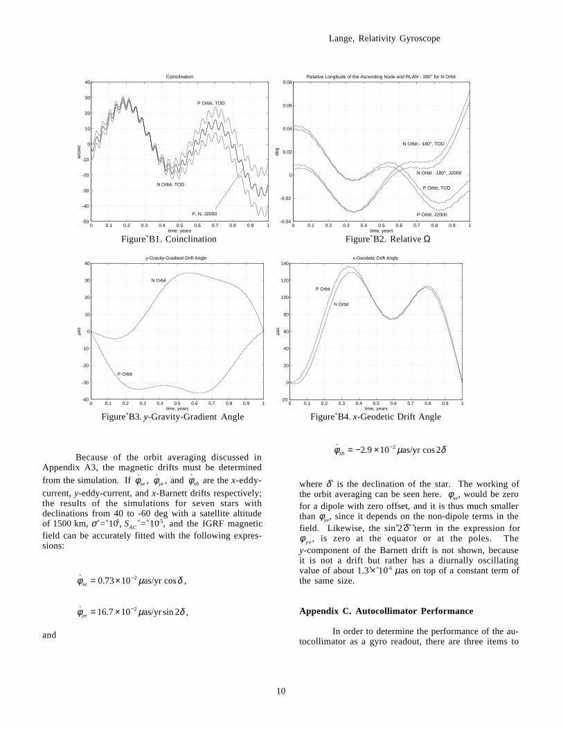
Figures B1 and B2 show coinclination, i', andlongitude of the ascending node, Ω, relative to Alnilamas the reference star. The coinclination is chosen sothat the average of the longitude of the ascending noderelative to Alnilam is approximately zero which causesthe y-gravity-gradient drift and the x-geodetic-relativitydrift to first grow and then return to zero at the end ofthe year as can be seen in Figures B3 and B4. Thecoinclination is shown both for the positive (P) andnegative (N) satellites and both relative to J2000 andrelative to the true earth of date (TOD). The curves rel-ative to J2000 lie on top of each other and cannot bedistinguished in the plots. The coinclinations relative tothe earth slowly diverge from the middle curve mostlydue to the precession of the equinoxes. It can be seenthat the average of the coinclination relative to J2000 isapproximately zero. In both Figures B1 and B2 the six-month period of the perturbation of the sun can beclearly seen; and in Figure B1, the two-week period ofthe perturbation of the moon is discernible. The two-week lunar period is also present in the longitudecurves, but it is weaker.

The initial coinclination and relative longitudewere chosen to also zero the x-geodetic drift because al-though a precision frame-dragging measurement wouldnormally be done in a separate experiment, it is still de-sirable to measure frame dragging simultaneously withthe geodetic drift; and the x-axis is the experiment axisfor frame dragging. Since the amplitude of the geodeticterm can be approximately 160 times as big as framedragging, it could be a significant error. At any ratethere is no other reasonable choice since both thex-gravity-gradient and y-geodetic drifts are not affectedto first order by the orientation of the orbit plane .


10

0 0.1 0.2 0.3 0.4 0.5 0.6 0.7 0.8 0.9 1-50

-40

-30

-20

-10

0

10

20

30

40Coinclination

arcs

ec

time, years

P Orbit, TOD

N Orbit, TOD

P, N, J2000

0 0.1 0.2 0.3 0.4 0.5 0.6 0.7 0.8 0.9 1

-0.04

-0.02

0

0.02

0.04

0.06

0.08Relative Longitude of the Ascending Node and RLAN - 180° for N Orbit

deg

time, years

P Orbit, TOD

P Orbit, J2000

N Orbit - 180°, TOD

N Orbit - 180°, J2000

Figure B1. Coinclination Figure B2. Relative Ω

0 0.1 0.2 0.3 0.4 0.5 0.6 0.7 0.8 0.9 1-40

-30

-20

-10

0

10

20

30

40y-Gravity-Gradient Drift Angle

µas

time, years

N Orbit

P Orbit

0 0.1 0.2 0.3 0.4 0.5 0.6 0.7 0.8 0.9 1

-20

0

20

40

60

80

100

120

140x-Geodetic Drift Angle

µas

time, years

P Orbit

N Orbit

Figure B3. y-Gravity-Gradient Angle Figure B4. x-Geodetic Drift Angle

Because of the orbit averaging discussed inAppendix A3, the magnetic drifts must be determined

from the simulation. If φxe , φye , and φxb are the x-eddy-

current, y-eddy-current, and x-Barnett drifts respectively;the results of the simulations for seven stars withdeclinations from 40 to -60 deg with a satellite altitudeof 1500 km, σ = 105, SAC = 10-5, and the IGRF magneticfield can be accurately fitted with the following expres-sions:

˙ . cosφ µ δxe = × −0 73 10 2 as/yr ,

˙ . sinφ µ δye = × −16 7 10 22 as/yr ,

and

˙ . cosφ µ δxb = − × −2 9 10 22 as/yr

where δ is the declination of the star. The working ofthe orbit averaging can be seen here. φxe, would be zerofor a dipole with zero offset, and it is thus much smallerthan φye, since it depends on the non-dipole terms in thefield. Likewise, the sin 2 δ term in the expression forφy e , is zero at the equator or at the poles. They-component of the Barnett drift is not shown, becauseit is not a drift but rather has a diurnally oscillatingvalue of about 1.3 × 10-6 µas on top of a constant term ofthe same size.

Appendix C. Autocollimator Performance

In order to determine the performance of the au-tocollimator as a gyro readout, there are three items to


11

check: the instrument noise equivalent angle, the zeropoint errors, and the scale factor errors.

Appendix C1. Autocollimator Noise EquivalentAngle

The autocollimator noise depends primarily onthe number of photons / sec in the beam and the size ofthe focused light spot or slit which in turn depend on the

design of the field-stop reticule. The performance re-ported by Jones for his optical lever [36], 14-µas/yr, wasachieved by having a large number of photons combinedwith a small effective slit size. For example to dividethe image of the focused slit by 3 × 106 in one second inthe presence of photon shot noise, approximately 1013

photons are needed. This is converted to an angle bydividing by the focal length; and if the focal length isabout 3 × 103 times the slit size, this gives 10-10 radiansor about 20 µas.

MinusPhoto-detector

PlusPhoto-detector

Field-Stop Mask

Detector Mask

Two-AxisDetectorMaskJones Original Single-Axis Reticule

Two-Axis Field-StopMask

Figure C1. Single- and Two-Axis Jones-Pfund Type Reticules

The Jones design uses a grid of slits as shownin Figure C1 to greatly increase the amount of light inthe beam while maintaining a very narrow slit andsmoothing out variations in the grid and photodetector.The field-stop mask is placed at the focal point of thecollimating lens next to the condensing lens in Figure 3,and the detector is masked with an identical maskexcept that the bars in the mask are displaced one halfof the slit width (Cf. Figure C1). When the image ofthe field-stop mask moves in a given direction, ituncovers the detector mask on one photodetector andcovers it on the other. Subtraction then generates a sig-

nal proportional to the displacement of the image of thefield stop, i.e. proportion to the mirror rotation. The con-denser lens focuses the image of the light source intothe interior of the collimating lens thus maximally defo-cusing the light source and guaranteeing a very uniformintensity across the detector surface as well as capturingmost of the light which passes through the collectorlens. Alternately the image of the light source may befocused on the optical flat, and this captures all of thelight which passes through the collector lens at the costof some uniformity across the detector surface.


12

The extension of the Jones' reticule to a two-axis autocollimator is also shown in Figure C1. Thenoise equivalent angle in radians/Hz1/2 of a two-axis in-strument with this reticule is given by w / 2 f n1/2 where nis the total number of detected photons in all four detec-tors, w is the width of one slit, and f is the focal length.If L is the length of the two-axis slits, the light-transmit-ting area is given by 2 L2 and is independent of w , sothat the noise equivalent angle is minimized by mini-mizing w / f. This is in stark contrast to autocollimatorswith a single square hole such as the ones that KenLorell and David Klinger built in our laboratories in thelate 1960s [49, 51]. (In their case, since n is pro-portional to w2 for a given illumination, w cancels in thenumerator and denominator.) The minimum value ofw / f in the Jones design is limited by the diffraction ofthe collimating lens; or in the case of the gyro readout,by the diameter of the optical flat, df . In order to deter-mine w / f, the diffraction pattern of the image of thefield-stop reticule in the image plane must be computed.Since the field-stop reticule is not self luminous, thelight will be at least partially coherent. To account forthis, the diffraction has been computed for two cases,incoherent illumination and completely coherent illumi-nation. For a flat diameter, df , of 5 mm, a focal lengthof 10 cm, and 0.5-micron light, 1.2 λ f / df is about 12 µ;and this provides a lower limit to the slit width. Thesurprising result is that the slits do not need to be verymuch wider than this limit. For example, when thediffraction calculation is done for a slit width of 25 mi-crons for incoherent light, the dark strip attenuates thelight by 2.5 × 10-2 at the center. For completely coher-ent illumination, the intensity alternates in the maskedregion with peaks and zeros with a period of about 2.5microns; and the attenuation at the central peak is about2 × 10-3. Also since the first zero of the coherent patternis about two microns past the edge, the edge is muchsharper for the coherent light as was first shown byAbbe. In either case the effect of the diffracted light onthe expression for the noise equivalent angle or on thescale factor of the instrument is small, and a slit widthof 25 microns is acceptable. Coherent illumination al-ways has a much smaller value at the center of themask; and with a fiber-optic bundle as the light source,coherent light will be possible so that the attenuation of2 × 10-3 should be regarded as more nearly correct. If aquarter section of the reticule is assumed to be 5 mm ona side, there will be 100 grid lines in each section; andthe maximum off axis angle of the ƒ20 optical systemwill be 2.9 deg.

With w = 25 µ and a focal length of 10 cm,w / f = 2.5 × 10-4; and for a total number of detectedphotons of 1013 per second, the noise equivalent anglefor each axis given by the above expression is8.2 µas/Hz1/2. The total beam intensity of1013 photons/sec corresponds to a photocurrent of 0.4 µA

in each of the four detectors making almost anyphotodiode detected-photon-noise limited. In one axis,the shot noise from 0.8 µA is 500 fA/Hz1/2; and thisshould be compared with: 1) the Johnson noise currentfrom the 10-M to 100-G feedback resistors of the opera-tional amplifier in the transconductance mode or the10-M current-source resistor which is 0.4 to 40 fA/Hz1/2 ,2) the noise current of typical FET or JFET operationalamplifiers which lies between 0.4 fA/Hz1 / 2 and10 fA/Hz1/2 , and 3) the shot noise from a photodiodewith a dark current of 3 nA which is 30 fA/Hz1/2 . The1/ f corners of the detectors and amplifiers typically liebetween 2 and 200 Hz so that 10- to 100-kHz choppingwhich any case is necessary to eliminate cross talk fromstray light among the four instruments (twoautocollimators and two transcollimators) completelyeliminates 1/ f noise.

Since an angle change at the mirror is multi-plied by two at the photodetectors, the maximum linearrange of the autocollimator is given by w / 4 f =6 × 10-4 rad = 13 arcsec. The maximum angle whichthe autocollimator must measure is about 0.2 arcsecarising from the flat misalignment error. This is one60th of the maximum linear range and corresponds to anoscillating reticule-image motion of 0.2 microns. 13arcsec gives a ratio of about 106 between the maximumlinear range and the smallest angle change which canbe measured with one second of averaging. This largeratio is particularly useful as it allows the zero to be setelectronically with a DC current source over a widerange of misalignment of the satellite maximum axis ofinertia. The DC gain at the input of the operational am-plifier is 2 nef / w, about 62 pA / mas; so that the highestDC output gain is 6 volts / mas. From the input gain,the 0.5 pA/Hz1/2 shot noise from two photodiodes corre-sponds to 8.1 µas/Hz1/2 which agrees with the noiseequivalent angle calculated above. Jones also had verylarge effective photo currents, and this explains why hewas able to operate at the photon-noise limit with veryprimitive detectors and electronics.

Appendix C2. Autocollimator Zero-Point Errors

The zero-point errors and drift of themechanics, photodetectors, and electronics are removedby spinning the satellite, and this is discussed in moredetain in Section 5 and Appendix F. In order to stay ineach other's linear ranges and to be consistent with theflat position errors, the two autocollimators should bealigned within about one arcsec of each other. Thesatellite maximum axis of inertia should also be alignedto the autocollimator zero points to this tolerance, andthis is accomplished with a satellite active mass-trimsystem [49]. The electronic zero can be set to bring thebalance of any DC offsets to less than one mas, and it isthe mass-trim system plus the electronic offset control


13

which guarantee that the largest autocollimator signalswill come from the flat misalignment error and thesatellite attitude motion.

Although the absolute zero-point drift in the au-tocollimator is removed by the satellite spin, it is stillinteresting to calculate what its value would be. It isdetermined principally by the thermal temperature coef-ficient of the materials and is of the order of 5 × 10-7

rad/K/meter = 100 mas/K/meter. The electronic offsetdrift with FET or JFET operational amplifiers is muchsmaller, of the order of 200 µas/K; and even bipolar op-erational amplifiers give an electronic offset of about8 mas/K. With absolute temperature control to 0.1 Kand a typical autocollimator size of 0.1 meter, the abso-lute zero point drift is not expected to exceed one mas.

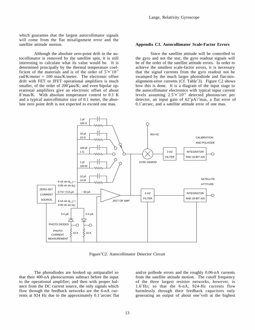
Appendix C3. Autocollimator Scale-Factor Errors

Since the satellite attitude will be controlled tothe gyro and not the star, the gyro readout signals willbe of the order of the satellite attitude errors. In order toachieve the smallest scale-factor errors, it is necessarythat the signal currents from the gyro readout not beswamped by the much larger photodiode and flat-mis-alignment-error currents (Cf. Table 3). Figure C2 showshow this is done. It is a diagram of the input stage tothe autocollimator electronics with typical input currentlevels assuming 2.5 × 1012 detected photons/sec perdetector, an input gain of 62 pA / mas, a flat error of0.1 arcsec, and a satellite attitude error of one mas.

10 K 10 KPHOTO

CURRENT

MEASUREMENT

10 M

10 pf

100 M

1 pf

1 G

100 pf

10 G

10 pf

100 G

1 pf

ZERO-SET

CURRENT

SOURCE JFET OP AMP

2-HZ

FILTER

INTEGRATOR

AND 16-BIT A/D

SATELLITE

ATTITUDE

INTEGRATOR

AND 16-BIT A/D

CALIBRATION

AND POLHODE

SYNC DEMOD

924 HZ

2-HZ

FILTER

PHOTO DIODES

0.4 µA 0.4 µA

6 nA sin ωG-St +

0.06 nA sin ωSt

6 nA sin ωG-St +

0.06 nA sin ωSt

0 TO +- 0.8 µA ~ 50 pA

Figure C2. Autocollimator Detector Circuit

The photodiodes are hooked up antiparallel sothat their 400-nA photocurrents subtract before the inputto the operational amplifier; and then with proper bal-ance from the DC current source, the only signals whichflow through the feedback networks are the 6-nA cur-rents at 924 Hz due to the approximately 0.1 arcsec flat

and/or polhode errors and the roughly 0.06-nA currentsfrom the satellite attitude motion. The cutoff frequencyof the three largest resistor networks, however, is1.6 Hz; so that the 6-nA, 924-Hz currents flowharmlessly through their feedback capacitors onlygenerating an output of about one volt at the highest


14

gain compared to 6 volts from the low frequency0.06-nA current. This means that the 400-nA and 6-nAcurrents do not coexist in an amplifier with the 0.06-nAattitude signal creating dynamic-range and linearityproblems. One volt, however, is large enough to stillprovide a useful gain-stabilizing or calibration signalsince the high stability of the capacitors and the gyrospin frequency combined with accurate measurement ofthe satellite roll frequency allows stable operation onthe descending slope of the frequency response curvebeyond the feedback network's cutoff frequency. At thelower gains, however, the 10- and 100-M networks havea cutoff frequency of 1600 Hz which allows the flat-misalignment signal to be seen at its full amplitude ifdesired. Once the flat misalignment error has beenmeasured with respect to the orbital aberration to a frac-tion of a µas; flat-misalignment which is stable to wellover 10-7 can take over from the aberration of starlightand provide continuous autocollimator calibrationthroughout the rest of the mission. The two 10-K re-sistors on the ground side of the photodiodes provide acontinuous measurement of the photocurrent and allowpossible variations in the light level to be compensated.The output of the operational amplifier is synchronouslydemodulated at the rotor-minus-satellite frequency of924 Hz to recover the calibration and polhode signals.The satellite attitude and zero-point error signals arecontained in the low frequency output of the operationalamplifier; and the satellite attitude is subtracted fromthe telescope signal to eliminate satellite motion fromthe star-gyro angle. The gain resistors must be switch-able to allow the autocollimator to operate at maximumlinear range for initial acquisition.

To achieve an accuracy of a fraction of a µas,the scale factors must be calibrated to this accuracy. Inthe case of the autocollimator this is not particularlycritical. Since the 924-Hz flat-misalignment and pol-hode errors can be filtered away, the largest signal inthe autocollimator is due to the satellite attitude motionand is of the order of one mas. A calibration accuracyof 10-4 gives a final error of approximately 0.1 µas, andeven a calibration as poor as one part in 103 would onlygive an error of about one µas. One problem is the pho-todiodes whose gain stability with respect to tempera-ture is relatively poor, about 10-3 / K; but with ten per-cent matching and temperature control to 0.1 K, theymore than meet a requirement of 10-4. Furthermore, theflat misalignment error will allow the autocollimator tostay in calibration at all future times.

Because an accuracy for the autocollimator of10-4 would be acceptable, most of the calibration can bedone on the ground before the flight. The principal prob-lem is the accuracy with which the reticule lines can belaid down, approximately 0.1 µ . Reticule errors areameliorated by the square root of the number of reticulelines and by about another factor of 10 by the continuity

of the marking process and the smearing of the imagedue to the diffraction of light and the optical aberrations.The telescope and autocollimator calibrations areclosely connected, and the details of the calibration arediscussed in Appendix G.

Appendix C4. Transcollimator

A transcollimator is an autocollimator with onlyone minor change. The focal length of the collimatinglens is shortened so that the exit beam is focused to apoint at the place where the center of the spherical gyrorotor would lie. When this is done, a translation, x, ofthe rotor perpendicular to the beam causes anequivalent rotation of, φ = x / a. This has the advantagethat almost all of the technology of autocollimators canbe carried over with very little change, and it allows aprecision optical measurement of rotor position with awide gap [1, 52]. Thus with a focal length of thecollimating lens such that the effective lever arm is 3cm when reflected from the sphere and a Jones reticulewith w = 1000 µ, the transcollimator noise equivalenttranslation will be 1.2 × 10-10 meter/Hz1/2 with a maxi-mum linear range of 200 µ for a rotor radius of 2.5 cm.

Within the accuracy with which the mass-trimsystem can center the center of mass of the satellite andwith which the drag-free control system can control thesatellite, the transcollimators operate with no distur-bance or offset signals so that scale factor errors are nota serious problem. In addition, there is no high-accuracy requirement for the measurement of theabsolute cavity position of the rotor. The only highprecision requirement is that the inertial component ofx -y translation be stable to 10-9 meters (See Ap-pendix A4).

Appendix D. Summary of the Technique forPlacing the Optical Flats on the Rotor

Polishing optical flats onto the rotor with an er-ror of 0.1 to 0.2 arcsec with respect to the zero-g maxi-mum axis of inertia is mostly a measurement problem.The basic method is to find the natural maximum axisof a newly polished sphere, polish an initial set of flatsperpendicular to this axis, measure the error of theseflats, and iteratively repolish the flats until the desiredaccuracy is obtained. The initial steps can be done inan air bearing to an accuracy of a few arcseconds, butthe final high precision measurements must be done inan electric bearing mounted on a three axis table whichtracks the spin axis of the rotor so that no torques needbe applied to keep the spin axis in the field of view ofthe autocollimators during the precision measurement.The techniques described here were worked out between1966 and 1972 [53, 54, 55, 33, 49].


15

The initial flats must be polished at the naturalmaximum axis of a new sphere because although theflats would determine the maximum axis of inertia on aperfect sphere, the initial moment-of-inertia differenceratio caused by surface irregularities and bulk inhomo-geneity of the material would compete with the maxi-mum axis caused by the flats to generate very large er-rors. If εpi is the initial permanent moment-of-inertia dif-ference ratio of a newly polished rotor and εpn is the newvalue after the flats are on the rotor, the error angle be-tween the apparent and zero-g maximum axes is givenby (εpi / εpn) sin θ cos θ where θ is the angle betweenthe initial and new maximum axes. If εp i = 10-6 andεpn = 15 (df / dr)

4 / 16 ≈ 10-4, the error could be as largeas 0.005 radians ≈ 1000 arcsec since εpi / εpn = 10-2. Inorder to reduce this initial error to about 30 arcsecwhere it can easily be removed by iterative polishing,the initial maximum axis of inertia must be located toan accuracy of 3000 arcsec or a little less than a degree.

This can be achieved in an air bearing in spiteof its potentially large torques which could cause an er-ror between the true zero-g maximum axis and the ap-parent maximum axis. The adequacy of an air bearingis an experimental result, but it may be explained asfollows: Since a symmetric rigid body executespolhodes with the apparent maximum axis of inertia atthe center, it can be seen from Euler's rigid-bodyequations that a rotor-fixed moment, M , rotates theapparent maximum axis of inertia by an angleφ = M / εphG ωG radians where h G is the angularmomentum of the spinning rotor whose maximum axis isbeing measured. An estimate of the magnitude of Mgenerated in an air bearing can be obtained bycomparing it with the inertially-fixed moment whichwould cause typical drift rates, d, of 10 to 100 deg/hr foran air-bearing rotor spinning at 300 rad/sec. This isuseful because the drift rates are much easier to see andhence are better known. Although the drift torques areinertially fixed and the maximum-axis error torques arerotor fixed, they can still be compared. This givesφ = d / εpωG which shows the great lack of sensitivity ofthe maximum-axis error. For 10- to 100-deg/hr drifts,this expression gives about 0.1 to one deg between theapparent and zero-g axes, but this is much larger thanthe actual error since the mechanisms by which an airbearing generates rotor-fixed moments is very weak.Thus the robustness of the principal-axis directioncombined with the relatively small magnitude of therotor-fixed air torques makes an air bearing acceptablefor the initial flat placement.

In a high-quality bearing, the offset of the rotorcenter of mass perpendicular to a vertical spin axis be-comes the more severe effect. The size of this offset

can be estimated from the lack of roundness of thesphere. If εerr ≈ 10-6 is the effective fractional polishingerror of the initial rotor which will be assumed to alsogive the offset when multiplied by the rotor radius, theapparent maximum-axis error from gravity acting on theoffset is given by 5 gεerr / εpaωG

2. For εp = 10-4, this isabout 50 arcsec in an air bearing with ωG ≈ 300 rad/secand about 0.12 arcsec in an electric bearing withωG ≈ 5800 rad/sec. These considerations were borne outby the experience in the late 1960s although those rotorswere commercial Beryllium-Copper spheres with an εerr

of about 10-4 giving an offset of 5000 arcsec in an airbearing. In spite of this, it was possible to align themaximum axis to about one arcsecond at a given tem-perature and rotor speed with laser mass trimming [54],and to measure the zero-g maximum axis to about 4arcsec [55]. (In an isotropic material there is nosensitivity of the principle-axis direction to temperaturein the zero-g conditions of space. It is only important inan earth-bound laboratory due to the temperaturevariation of the center of mass relative to the effectivecenter of support.)

Thus to locate the initial maximum axis of iner-tia of a newly polished sphere, the rotor is placed in anair bearing with eddy-current torquing coils and/or a pairof jets to provide the spin motor. The rotor can bedamped by rubbing it with a small soft brush or the pol-hodes can be traced out by putting successive ink dotsat the spin axis. This generates a marked rotor whichlooks like the one in the frontispiece of Deimel's book[56] and locates the maximum axis to an accuracy of afew degrees. Next a grid (which will be covered upwhen the flat is polished on the rotor) is inscribed overthis spot, the rotor is cleansed, and a short perpendicularsynchronizing line is drawn on the equator to opticallytrigger a signal synchronous with rotor spin. The rotor isthen placed in an air bearing which also has three pairsof orthogonal eddy-current torquing coils that can applya moment perpendicular to the spin axis, and the rotor isdoubly illuminated with white DC light from an ordinaryincandescent lamp and with a stroboscope which is syn-chronized to the spin speed. When the rotor surface isobserved under a microscope, the spin axis can be seenas a set of concentric circles of the white DC light re-flecting off of tiny surface imperfections; and the pol-hoding causes the surface as seen in the strobe light tomove under the microscope crosshairs centered on theconcentric circles much like a city in the sights of abombardier in an old WW II movie. The maximum axisis to the left of the motion; and by hooking the torquingcoils to a joy stick so that it generates rotor-fixedtorques proportional to its displacement, a visuallysteered active damper can be constructed which willdrive the spin axis to the maximum axis of inertia [53].Using this technique, the location of the apparent maxi-


16

mum axis on the inscribed grid can be found to a fewarcseconds.

Next two optical flats are polished on the rotor,and it is placed in an electric bearing mounted on athree-axis table with an autocollimator at each end.The error in the flat placement is then determined[54, 55], and the flats iteratively polished to eliminatethe error. If necessary, the difference between theapparent and zero-g maximum axes can be determinedby plotting the flat error as a function of spin speed; butas seen above, the error in the electric bearing is onlyabout 0.12 arcsec. In addition the spin axis can be ro-tated to be either vertical or horizontal, and the electricbody-fixed moment determined. The anticipated im-provement in accuracy over the results of the 1960scomes about by improved rotor polishing (now routinelydone to about one µin, i.e. about a part in 106 [28]), bythe use of an electric bearing with the correspondinglyhigher rotor spin speeds and well defined disturbingtorques, and the three-axis table which eliminates theneed for a torque motor during the measurements andwhich allows the spin axis to have any orientation be-tween horizontal and vertical. Using these techniques,the zero-g axis can be measured to better than one masand the flats can be aligned with this axis to at least 0.1or 0.2 arcseconds.

Appendix E. Telescope Performance

Appendix E1 Telescope Noise Equivalent Angle

The telescope noise equivalent angles are cal-culated using the method of spectral integration, i.e. byintegrating the product of the star, photodetector, andfilter spectral responses rather than the monochromaticapproximation which uses the peak wavelength of thestar. It is better to integrate over the spectral responsessince the monochromatic approximation underestimatesthe photon noise by about two thirds. The method ofspectral integration and the formulas for the noiseequivalent angles are derived in [43].

Although the photon beam is divided amongmultiple detectors, it is convenient to express the noiseangle in terms of the total number of photons detectedby all detectors. The number of photons detected de-pends on the quantum efficiency, η (λ ), of the detectorwhich is just the responsivity scaled by hc / λ e so that

η λλ

λλ

λ

λλ

λ

( ) ( ).

( )

. ( )

= = × −

=

−hc

eR R

R

1 2398 10

2 2543

6

0

watt mAmp

wattsAmp

E1

where R(λ) is the detector responsivity in Amps/watt, eis the electronic charge, and λ 0 = 5500 A°. Since astar's visual magnitude is defined by a photon flux, S, at5500 A° such that S(5500 A°) = 10-m V / 2.5 × 1.053×107

photons/sec/m2/A°; the total number of photons/seconddetected by all detectors, n, is given by

n A S R We

edT

mnqe

x

xV=

−−

−∞

∫1011

2 5 05

0

0/ . ( ) ( )λ λ λ

λλ E2

where Snqe = 1.053×107 photons/sec/m2/A° × 2.2543watts/Amp = 2.373×107 watt-photons/sec/m2/A°/Amp,W(λ) is the IR window transmission function, and AT isthe effective area of the telescope primary calculatedbelow. x = hc / λ kT and x0 = hc / λ 0kT where T is thetemperature of star so that the incident flux has beenscaled to match the visual magnitude of the star at5500 A°. Using Equation E2, the noise equivalent angleof a single axis is given by

θ

πλ λ

λλλ

λ

n

T Tm

nqe

x

x

n

A D SR W e

edV

=

−−

−∞

∫

1 22

2 1011

2 5 05

0

0

.

( ) ( )/ .

E3

Table E1 shows the results of the noise cal-culations for the most likely candidates for the referencestar. The number of detected photons per second, thedetected-photon noise equivalent angles, and the detec-tor-dark-current noise equivalent angles at room temper-ature are shown for two detectors; a Burle IndustriesGallium Arsenide C31034A photomultiplier and aHamamatsu R4632 photomultiplier. The C31034Awhich is a Gallium Arsenide device has especially highambient-temperature dark current. For this reason it istypically operated at –30° C, but the number of detectedphotons in this application is so large that the ambient-temperature dark noise of the C31034A is acceptable.The effective primary area is determined as follows:counting the Schmidt corrector, the primary and sec-ondary mirrors, four tipping plates, the pyramid prism,the refocusing reflectors, and the refocusing lenses;there is the IR window with a transmission of 0.75(assuming W (λ ) = 1), four reflecting surfaces with atransmission of (0.97)4, six bulk absorbtions with atransmission of (0.9995)6, and twelve refractive coatingswith a transmission of (0.985)12 making a total transmis-


17

sion in the optics of 0.552. Counting a central obscura-tion with a diameter of 10 cm, the total telescope

transmission becomes 0.518 giving an effective area of0.065 m2 down from 0.126 m2.

Name Declination Det Ph/sec Det Ph Dark Det Ph/sec Det Ph Dark(deg) Burle Ga As Noise Noise Hamamatsu Noise Noise

C31034A µas/Hz1/2 µas/Hz1/2 R4632 PM µas/Hz1/2 µas/Hz1/2

Achernar -57.24 1.01E+09 7.7 1.8 9.80E+08 6.5 0.021Rigel -8.202 9.34E+08 9.1 3.2 7.40E+08 8.8 0.032Capella 46.00 6.34E+08 15 10.6 3.08E+08 19 0.106Mintaka -0.2992 2.56E+08 14 6.4 2.91E+08 11 0.064Nair al Saif -5.917 1.58E+08 18 10.3 1.81E+08 14 0.103Alnilam -1.202 3.86E+08 12 4.6 4.19E+08 9 0.046Canopus -52.70 1.48E+09 8.5 3.0 9.45E+08 9.2 0.030Sirius -16.72 3.43E+09 5.1 1.0 2.48E+09 5.2 0.010Procyon 5.225 5.02E+08 16 10.2 2.93E+08 18 0.102Mimosa -59.69 5.79E+08 9.6 3.0 6.35E+08 7.6 0.030Hadar -60.37 1.01E+09 7.4 1.8 1.07E+09 5.9 0.018Arcturus 19.18 7.23E+08 15 10.8 3.13E+08 19 0.108Rigel Kent -60.84 6.98E+08 14 8.2 3.79E+08 16 0.082Ve ga 38.78 8.90E+08 9.9 3.9 6.53E+08 10 0.039

Table E1. Detected-Photon Noise for Selected Bright Stars and a 40-cm Telescope.

The stars in Table E1 generally have ac-ceptable noise performance with both types ofphotomultiplier, but they naturally fall into certaingroups which are useful for different mission emphases.The low declination stars: Mintaka, Nair al Saif,Alnilam, Procyon, and Rigel give the best drift perfor-mance; and Mintaka or Alnilam would be best for afour-satellite mission doing a simultaneous high-precision geodetic and frame-dragging experiment usingonly one star. This is because their very smalldeclinations guarantee that the declination-timecondition, the product of declination and experimenttime must be less than 8 (rs / Re)

2 / 3 J2 n in a polar orbit,e.g. 450 arcmin-years at 1500 km [27, 2], is fulfilled forlong missions which in turn guarantees that the gravity-gradient-drift angle will also return to zero in the frame-dragging case. The hot, distant, O and B stars: Alnilam,Mintaka, and Rigel have the least inherent proper mo-tion uncertainty. The very hot O and B stars: Mimosa,Nair al Saif, Mintaka, and Alnilam would have betternoise performance if acceptable UV optics andphotomultipliers could be found. The very close stars:Rigel Kent, Sirius, and Procyon would give the bestchance of seeing earth-like planets (Cf. Appendix H5),but the intermediate-distance stars: Achernar, Capella,Arcturus, and Vega might also reveal small planets.The medium-temperature main-sequence stars: Sirius,

Vega, and Rigel Kent would be of the most interest ifearth-like planets were detected around them.

Appendix E2. Telescope Zero-Point Errors

As with the autocollimator, the telescope zero-point errors are eliminated by spinning the satellite (Cf.Section 5 and Appendix F). Since the telescope looksat inertial space, however, any change in the effectivecenter of the incoming light is fixed in inertial spaceand is not removed by spinning the satellite. In additionto proper motion, subtraction of the results of twoexperiments looking at the same star also suppressesthese errors. They include any change in thebackground light of the very faint distant stars andgalaxies (a remote supernova or quasar flare), varyingbackground nebulosity, any change in the centroid ofthe star's light, polarization of the starlight, gravitationalbending of the incoming light by the sun, etc. Somestars have a detectable polarization in their light, andthis would be seen in the telescope via transmissionthrough the tipping plates. This error is theoreticallyzero since it is at twice roll frequency, but a subhar-monic component could be generated by tipping plateoscillations for example. In any event all common-


18

mode problems are eliminated to the accuracy of the in-struments by subtraction.

Although like the autocollimator the zero-pointoffset drift is removed by the satellite spin, it is stilluseful to know its size. The absolute offset drift of thetelescope is determined principally by the thermal tem-perature coefficient of the materials and is of the orderof 5 × 10-7 rad/K/meter = 100 mas/K/meter. Theelectronic offset with FET or JFET operationalamplifiers is much smaller, of the order of 0.05 µas/K.With absolute temperature control to 0.1 K and a typicaltelescope size of one meter, the absolute zero point driftis expected to be less than 10 mas.

Appendix E3. Telescope Scale-Factor Errors

In order to keep the telescope scale-factorerrors in bound it is necessary to operate the telescopeas close to null as possible. For an accuracy of 0.2 µasand a limit on the linear range of 106, the apparentangle between the gyro spin axis an the star cannotexceed 0.2 arcsec. This is accomplished by using theorbital aberration of starlight to cancel the relativitydrift. Since the annual aberration of starlight can be aslarge as 40 arcsec, high precision measurements in nullcan only be made at the beginning and end of theexperiment, one year apart, when the annual aberrationreturns to its starting value. Using the telescope coarsetipping plates, measurements could be made andaveraged over the whole year; but high-precision datawould only be taken at the beginning and the end.

0 0.1 0.2 0.3 0.4 0.5 0.6 0.7 0.8 0.9 1-25

-20

-15

-10

-5

0

5

10

15

20

25Annual Aberration versus Right Ascension

arcs

ec

Time, years

a y

a x , RA=0°

a x , RA=45°a x , RA=90°

Figure E1. Annual Aberration Signals for Various Star Right Ascensions

With this strategy, the important question be-comes how long does a ±0.2 arcsec null last, i.e. howmuch averaging time is available for the telescope andautocollimator noise equivalent angles? In the star co-ordinate system with the z-axis toward the star, thex-axis making the smallest angle with north, and ωa

equal to the earth's mean annual orbital rate; the non-spinning x- and y-telescope annual aberration angles aregiven by

a

v

ct txa

moa a= −

+[ ]−sin 1 s sω α ω α εc c c E4


19

and

a

v

ct tya

moa a= −

+ −( )[ ]−sin 1 s s s s sω δ α ω δ ε δ α εc c c c

E5

where α and δ are the star's right ascension and decli-nation, ε is the obliquity of the ecliptic, and vm o is thevelocity of the earth in its orbit which is assumed to becircular. Figure E1 shows plots of ax a and a y a for adeclination of zero degrees and three right ascensions,0, 45, and 90 degrees. It can be seen that each aberra-tion curve has a maximum or a minimum twice per yearwhen the aberration changes only slowly, and the aber-ration angle remains within ±0.2 arcsec for about 23days for x and about 36 days for y. For small declina-tions and stars close to the equinoxes, the x - andy-curves are almost in phase, and it possible to remainwithin ±0.2 arcsec for 23 days in both axes. For starswith right ascensions other than zero or 180 deg, thex-aberration angle dephases from the y-angle, drasticallyreducing the time that both axes are in null. In the ex-treme case of 90 deg, the time in null is only two orthree days for some stars giving a very small averagingtime. There is a way around this problem, however,such that the maximum null time of 23 days may be hadfor a star with any right ascension. To see this, the ex-act method of cancellation of the relativity drift by theorbital aberration must first be considered.

It can be seen from Table 1 that orbitalaberration can be used to exactly cancel the relativitydrift at any altitude above 1560 km and to cancel it witha maximum error of 0.8 arcsec at altitudes above 1000km. To effect this cancellation the measurements aremade in different parts of the orbit at the start and endof the experiment. The gyro alignment is initializedwhen the satellite is over the ±90-deg points withrespect to the star where the orbital aberration is zero,i.e. the angle measurement between the star and the gy-roscope is averaged during the approximately 90seconds at each 90-deg point while the aberration iswithin the 0.2 arcsec null. This is repeated for as manyorbits as possible until the change in the annual aberra-tion makes it no longer possible to come into null. Atthe end of the year the angle between the gyro and thestar is read when the orbital aberration is close to themaximum, i.e. when the satellite is close to the equatordefined by the star (zero-degree point). Since orbitalaberration and the geodetic relativity drift are in thesame direction, they then cancel one another. Againthe number of orbits where data can be taken is limitedby the change in the annual aberration. In order to getaround the difficulty of dephasing and have the maxi-mum time that the annual aberration is within ±0.2arcsec, the experiment is initialized at one of the two

times per year when the x-aberration angle is at amaximum or a minimum giving the full 23 days in thataxis. In the case of the y-axis, the aberration angle israpidly changing and the null is much shorter than 23days for stars that do not lie close to the equinoxes. They-axis, however, is the experiment axis; and the annual-aberration y-angle can be canceled at each pass withthe orbital aberration by moving the point at which datais taken a little bit before or after the exact position atthe ±90-deg points or at the zero-degree point. In thisway any star can have the full 23 days of null. For thefirst in the series of one-year experiments where therelativity geodetic drift and the orbital aberration arealmost equal, this option is not available at the end ofthe experiment at the zero-degree point; but this is not aserious drawback since the time in the orbital null isabout five times as long at the zero-degree point, 900seconds compared to 180 seconds. As the series of one-year experiments progresses and the altitude is raised in100-km increments, more and more freedom becomesavailable at the zero-degree point to advance or retardthe measurement to cancel the annual aberration.

Thus 23 days are available at the ±90-degpoints with about 12.4 orbits per day and 90 seconds ateach point, and this gives a total averaging time ofabout 26,000 seconds counting the fact that the totalmust be reduced by about half because the full ±0.2 arc-sec is not available at the edges of the cancellation. Atthe zero-deg point, this time is five times larger,130,000 sec. In the case of the autocollimator, thetimes are further cut in half by the chopping. If thenoise equivalent angle of the telescope is 10 µas/Hz1/2,the error after 26,000 seconds of averaging is approxi-mately 0.05 µas. Having sufficient averaging time toalways be able to make the telescope measurementswithin a range of ±0.2 arcsec lessens the severity of thescale-factor problem by a factor of 100 to 200 over anexperiment which averages over the entire year.

There is an additional advantage to setting thestart and end times at the maximum or minimum valuesof the x-aberration. These occur when the earth, sun,and projection of the star into the plane of the eclipticall lie in a straight line. When the order is sun-earth-star, the sun shines on the back side of the spacecraft sothat the telescopes are in the vehicle's shadow when theprecision data is taken; and the satellite itself is mostlyon the night side of the earth. The angle between thesun and the –z-axis of the vehicle is equal to theecliptic latitude of the star. Table E2 shows thestart/end date and the ecliptic and galactic latitudes ofselected bright stars. It can be seen that in most cases,the sun is almost directly behind the spacecraft becausethe ecliptic latitude is small. The galactic latitude hasno relevance to the sun angle, but it is also shownbecause it gives an idea of the density of faintbackground stars.


20

Star RA Declination Start/End Ecl Lat/ Gal Lat(deg) (deg) Date Sun Angle

Achernar 24.425 -57.25 19-Oct -59.4 -58.7Rigel 78.643 -8.202 11-Dec -31.1 -25.0Capella 79.171 46.00 12-Dec 22.9 4.73Mintaka 83.001 -0.2992 15-Dec -23.6 -17.5Nair al Saif 83.858 -5.917 16-Dec -27.4 -18.5Alnilam 84.053 -1.202 16-Dec -24.5 -17.0Canopus 95.988 -52.68 27-Dec -75.8 -25.1Sirius 101.29 -16.72 1-Jan -39.6 -8.65Procyon 114.83 5.233 28-Jan -16.0 13.3Mimosa 191.93 -59.70 2-Apr -48.6 3.17Hadar 210.96 -60.37 23-Apr -44.1 1.21Arcturus 213.92 19.18 26-Apr 30.7 68.9Rigel Kent 219.90 -60.83 2-May -42.6 -0.738Ve ga 279.23 38.78 30-Jun 61.7 19.0

Table E2. Start Date and Sun Angle of the Bright Stars

The question now arises how to design the tele-scope to cover the linear range from zero to 0.2 arcsecwith a scale-factor error of the order of 10-6. This can bedone by reading out the rotation angle of two servo-con-trolled tipping plates which center the diffraction spoton the pyramid prism. If the telescope has a focallength of 10 meters, the movement of the image spot atmaximum deviation of ±0.2 arcsec is ±10 microns. Forsmall angles, the lateral displacement of the beamcaused by a tipping-plate rotation, θ, is given by θ t (n – 1) / n where t is the thickness of the plate and n is itsindex of refraction. For n = 1.5, a 150-micron thick tip-ping plate can zero a deviation of ±10 microns with amaximum rotation of approximately ±10 degrees. In or-der to avoid the problem of converting an analog signalwith an accuracy of 10-6 or better which would requirean AD converter with at least 20-bit accuracy, the tip-ping plate is rigidly connected to an 11-bit angle en-coder with 2048 divisions per 20 degrees at the 11th bit.The last bit is divided by an analog signal which is ob-tained from a capacitive coupler also consisting of 2048plates per 20 degrees (18432 in the full circle) on theouter radius of the encoder. This analog signal is con-verted with a 12-bit AD converter giving a total of 23bits ≈ 8.4 million without requiring a 23-bit AD con-verter. This corresponds to a resolution of approxi-mately 0.05 µas in reading ±200,000 µas. In addition tothe analog signal from the last bit division, the tipping-

plate servo mechanism makes errors of the order of30 µas in centering the diffraction spot on the prism.Because of this, it is necessary to correct the analogmeasurement with the raw light signal to get the lastone or two orders of magnitude of accuracy.

The accuracy with which the 8.14-µ wide platescan be laid down on the angle encoder is about 0.1 µwhich corresponds to an error of about 0.2 arcsec at a ra-dius of 10 cm. Although full scale corresponds to ±10degrees for the tipping plates, the entire circle of the an-gle encoder would be used for the capacitive divider.With 18432 plates, the 0.1-µ error would be reduced bya further factor of about (18432)1/2 ≈ 136 by smoothing,so that the final angle-encoder error would be of the or-der of 2 mas. Since the amplification of the tippingplate is n f / t (n – 1) = 2 × 105, an angle-encoder error of2 mas corresponds to a readout error of 0.01 µas .Because of these considerations and the symmetry prop-erties of a full circle, only very minimal calibration ofthe angle encoder is required. The cross-axis bearingstability requirements are similar. Assuming a 10-cmaxis, a bearing-centering stability of about 0.1 µ or 4 µintranslates into an angle-encoder error of 0.2 arcsecwhich in turn corresponds to a readout error of one µas.This would also be reduced by about one or two ordersof magnitude by the averaging of the bearing noise.


21

PYRAMID PRISM

REFOCUSING REFLECTOR

REFOCUSING LENSES

D1ID2I

D1Q

D2Q

CHOPPER WHEEL

x = Q + Iy = Q - I

CHOPPER MOTOR

xy

Figure E2. Telescope Readout Light Path

The photodetectors for the telescope have thesame stability problem as with the autocollimator, andin the case of the telescope there is no calibratingsignal to hold the gain stable. The problem can besolved, however, by chopping which also eliminates the1/ f noise. Figure E2 shows the detector arrangementand the light path after the prime focus at the tip of thepyramid prism10 . In the figure the focused light from

10 A beam splitter and two roof prisms [53] couldbe used to process the image instead of the pyramidprism, but this has the additional complication of apossible curvature of the roof prism edge. If theroof prisms were to be used, the light path from asingle roof prism would be the same as one half ofFigure E2 with only one chopper and one set ofreflectors and detectors. A system with two roofprisms has the advantage that the prisms areperhaps easier to manufacturer, and the tipping

the telescope arrives at the point of the prism down-wards along a line perpendicular to the page. The tip-ping plates (not shown) are just above the pyramidprism. The diffraction spot is focused onto the point ofthe pyramid prism for maximum sensitivity and then thepairs of split beams are refocused on the detector D1 bythe concave reflectors and the refocusing lenses. A fan-blade chopper wheel exactly cuts off one of the twobeams, and the interrupted beam is reflected to detectorD2. Thus D1 and D2 alternately see the plus and minusbeams, and the servo error signal is always generatedfrom the same detector. Detector scale-factor drift thenplays an insignificant role since the tipping-plate servoholds the two beams in close balance.

plates would be single-axis devices. The noise forthe roof prisms is 21/2 greater than for the pyramidprism, and the noise values in Table E1 are for apyramid prism with only one detector or roof prismswith detectors D1 and D2.


22

The chopper shaft frequency is about 0.5 Hzwhich combined with a 10-blade wheel gives achopping frequency of 5 Hz. The very low shaftfrequency combined with precision bearings andprecision wheel balancing eliminates vibration as aproblem. The chopper has many other sources of error,but the system can be designed so that they do noteffect detector D1 because its beam passes the chopperunimpeded. This is done by blocking the measurementwhen the beam is switched so that switch-over errorsdue to blade imperfections and the finite beam widthare eliminated. In addition to vibration, the choppererrors are: unequal angular size of the openings,misalignment of the wheel plane with respect to thechopper shaft, misalignment of the shaft bearings withrespect to the optical axis, bearing noise,desynchronization of the wheel angle with respect to thedemodulation signal, and wheel flatness errors. Theseerrors mostly affect D2 but not D1 because they affectthe centering and the focus of the light which falls onD2 since it is reflected from the wheel surface, and theycould potentially require that the data from D2 not beused.

In addition to scale-factor errors caused by thereadout, coma in the telescope also generates a scale-factor error. The Schmidt telescope can be designed to

reduce coma to about 100 µas / arcsec-off-axis, and therest can be removed by calibration. Because the tele-scope signal is chopped, the absolute stability of thescale factor is determined principally by the thermal ex-pansion coefficients of the materials and is about5 × 10-7 / K for a truss made of Invar.

Appendix F. Roll-Coupled Zero-Point Errors andDrifts

Since satellite spin is used to separate the zero-point errors and drifts from the science data, any contri-bution to an instrument zero point which had a compo-nent at the satellite roll frequency would cause a mea-surement error. If the amplitude of any such term driftedover the course of the year while the experiment was inprogress, it would constitute an error in the experimentalresult. For this reason the gyro and the instruments,telescope and autocollimator, are surrounded by a ther-mally insulated, mechanically and electrically isolatedenclosure. The instrument zeros shift because of me-chanical deformation and because of change in theelectrical balance of the photodetectors and their opera-tional amplifiers. Table F1 shows a summary of theresults of the calculations of the roll-coupled zero-pointerrors.

Roll-Coupled Zero-Point Errors Summary:(µas)

Thermal Thermal deformation of the truss structure 5.7E-04Leakage Thermal deformation of the telescope 5.7E-04

Thermal deformation of the autocollimator 5.7E-05

Mechanical Transmitted satellite thermal deformation 0.01Leakage Thruster-caused mechanical deformation 4.5E-06

Tipping-Plate-caused mechanical deformation 5.0E-13Subharmonic tidal deformation 4.1E-07

Elec. Leakage Power supply roll frequency ripple, see text. 0

Telescope Telescope photomultiplier unbalance 1.1E-08Electronic Offset Telescope op amp, input offset current 5.5E-07

Telescope op amp, input offset voltage 5.5E-10

Autocollimator Autocollimator photodetector unbalance 5.5E-08Electronic Offset Autocollimator op amp, input offset current 5.5E-10

Autocollimator op amp, input offset voltage 5.5E-10

Zero-Point Error RSS 0.010

Table F1. Roll-Coupled Zero-Point Errors


23

The first group of errors is the distortion of thetelescope and autocollimator frames and of the trussstructure which supports the instruments caused by tem-perature gradients inside of the enclosure which oscil-late at roll frequency. The deformation of the truss cancause an error angle between the telescopes and the au-tocollimators, and a deformation of an autocollimator ora telescope causes a direct mechanical shift of its zeropoint. If the heights and widths of the instruments areroughly equal, then the angle error is simply the temper-ature coefficient of expansion of the material times thetemperature difference. The thermal expansion coeffi-cient used was that of Invar, 5 × 10-7 / K. In addition toInvar, Zerodur glass with a thermal coefficient of expan-sion of 5 × 10-7 / K can be used for the telescope optics;and in difficult situations, Superinvar with 1 × 10-7 / K isavailable.

The second group consists of the errors causedby mechanical deformation in the satellite which cou-ples to the trust structure inside of the enclosure whichmounts the telescopes and the gyro assembly includingthe autocollimators and magnetic shield. The largest er-ror in this group comes from the thermal distortions ofthe satellite structure outside of the enclosure which aretransmitted mechanically to the truss structure on the in-side. To keep this error within bounds the support of thestructure must be carefully designed. At this time forthe purpose of calculating the size of this effect, it willbe assumed that the truss structure is coupled to the restof the satellite at a single point. Once in space this isnot a problem; but to survive launch, other supportpoints are required. It is assumed that these additional

support points are severed just after orbit insertion. Thesatellite distortion angle is assumed to be given by thethermal coefficient of expansion of Aluminum,2.5 × 10-5 / K, times the assumed roll-frequency ampli-tude of the temperature of the satellite structure, 0.1 K.Although the outside skin temperature variation wouldbe about 10 K, the structure is temperature controlled toabout 0.1 K in roll. The transmission of the structuraldeformation to the inner truss was calculated by a finite-element model and was found to be about 0.01 µas [57].

The balance of the errors are very small, butthey are included for completeness. The thruster defor-mation assumes that the trust is deformed by the forcefrom the drag-free thrusters which would have a compo-nent at roll. The magnitude of the thruster forces wastaken from the drag at a solar maximum or the solar ra-diation pressure which are about the same magnitude.The tipping-plate error comes from the fact that it mustoscillate at roll frequency and the reaction torque dis-torts the truss. The tidal distortion is theoretically zerosince it occurs at twice roll frequency, but there mightbe some conceivable mechanism where the oscillationsdid not return to exactly the same point causing a sub-harmonic term. The amplitude in the table was calcu-lated by multiplying the amplitude of the tidal distortionby 0.001 as an estimate of the subharmonic amplitude.The amplitude of the electronic offsets were calculatedin the standard way by multiplying the temperature sen-sitivities of the offset voltages and currents by the rolltemperature amplitude and translating this into theequivalent angle.

Temperature and Temperature Gradient in Roll K or K/meter

Temperature waves through the insulated enclosure walls 3.84E-09Temperature waves through 33 cm of copper power leads 3.99E-09Roll-temperature amplitude at the telescope IR window 1.00E-11Roll-temperature amplitude at the vacuum exhaust port 1.00E-12Roll-temperature due to roll ripples on the power bus 2.49E-101100th orbital harmonics 3.47E-12

RSS Roll-Temperature Amplitude 5.54E-09

Table F2. Temperature and Temperature-Gradient Amplitudes at Roll Frequency

Finally the roll-frequency variations of tempera-ture and temperature gradient inside of the thermal en-closure must be calculated. Table F2 shows the resultsof this calculation. Temperature influences from roll-coupled heating of the spacecraft by the sun and theearth's IR can enter the enclosure as temperature waves

through its insulated walls, along the copper in thepower and communication cables, through the telescopeaperture, through the vacuum exhaust ports, and by in-ternal heating caused by ripples on the power bus. Inaddition, approximately the 1108th harmonic of the orbitfrequency lies at the roll frequency. Using a square-wave model there is a small outside temperature varia-


24

tion equal to approximately the orbital variation inspacecraft skin temperate divided by 1100. This is avery tiny effect; but the question occasionally comesup, so it is included here.

The calculations shown in the table only givethe roll temperature amplitude at the output of the leak-

age source and do not take into account the heat capac-ity of structures or temperature waves inside of the en-closure. These would have the effect of further attenuat-ing the temperature amplitudes. No distinction is madein the calculations between temperature and tempera-ture gradient since the size of the satellite is of theorder of one meter.

10-4

10-3

10-2

10-1

100

10-20

10-15

10-10

10-5

100

Frequency, Hz

Atte

nuat

ion

Insulation Attenuation versus Frequency

2 cm (66 cm Cu)

1 cm (33 cm Cu)

rho=200 kg/m^3, C=1880 J/kg-K,

kappa=0.04 watts/m-K

Orbit 10 min GP-B 1 min AC-USG

Figure F1. Temperature Wave Attenuation versus Satellite Roll Frequency, ωS / 2 π

The most important roll-temperature source is tempera-ture waves through the insulated walls. The calculationof this effect is done in the classical manner using theresult of wave attenuation calculated from a sinusoidalinput to the diffusion equation. The characteristiclength is given by L = (2κ / Cρ ωS)

1/2 where κ is thethermal conductivity of the insulation, C its specificheat capacity, and ρ its density. The roll-temperatureamplitude is then given by the outside temperatureamplitude times exp(-tw / L) where tw is the thicknessof the insulation and the outside temperature variation isassumed to be 10 K. In this calculation tw was taken asone cm, and for typical insulation, κ as 0.04 watts/m/K,ρ as 200 kg/m3, and C as 1880 J/kg/K resulting in a

characteristic length of 0.46 mm. An interesting point isthat the characteristic length for copper is 15 mm, i.e.only about 33 times as long although the conductivitydiffers by orders of magnitude. This means that a powercable of length 33 cm has the same attenuation as aninsulating wall one cm thick and allows temperaturevariations from this source to be suppressed. The otherinteresting thing about this calculation is that becauseof the exponential, a loglog plot of the attenuationversus frequency is not a straight line but an eversteepening curve in the downward direction. Thismeans that beyond a certain roll frequency, roll tem-perature variations essentially vanish; and conversely,too slow a roll frequency does not achieve very much.


25

This is shown in Figure F1. For this reason the satelliteroll frequency has been chosen at one rad/sec, and it isbasically this high roll rate which eliminates many ofthe problems from roll-coupled errors.

The telescopes are completely enclosed in thethermal enclosure and look into space through and IRwindow which is designed to prevent heat leaking out ofthe enclosure and to attenuate roll temperature varia-tions entering the cavity. Outside of the enclosure, thetelescope field of view is protected from sunlight andearth albedo and IR by a cylindrical shield one or twometers long with about ten equally-spaced flat ring-shaped baffles inside. These shields were developed forearth-observing satellites and are available as off-the-shelf items. They are stowed for launch in collapsedform like a stove-pipe hat and are deployed in orbit withan internal spring. They can also have a shutter at theend which can be closed if needed, for example, at thesix-months point when the sun can shine almost directlyinto the telescope as shown in Table E2. The roll-temperature amplitude at the telescope window iscalculated by assuming an IR window attenuation of0.01 and an attenuation of 0.1 per baffle. Roll-coupledIR radiation into the telescope from the sun shining intothe end of the shield is then attenuated by 1011. Inaddition to direct sunshine inside of the end of theshield, the sun could also heat the side of the shield atroll frequency. These sources are unlikely to be aproblem during the precision measurements in nullsince, as explained in Appendix E3, the experiment canalways be started and ended with the sun almostdirectly behind the spacecraft. For year-roundmeasurements, they can be eliminated either by doubleshields or a reflective coating on the shield.

The power-bus ripples can be completely elimi-nated by having two batteries inside of thermal enclo-sures of their own which are alternately used while theother one is being charged from the power bus. Becauseof the extra batteries, it would be desirable not use thissolution; but it provides a backup in case the power buscannot be sufficiently regulated so it can be used di-rectly. If the power-bus is used, the roll rippleamplitude must be held below approximately onemicrovolt.

Appendix G. Instrument Scale-Factor CalibrationAccuracy

The coefficients of the calibration polynomialsin Section 6 are determined by comparing known inputangles with the telescope or autocollimator mea-surements. There are two instruments and only one cali-bration signal; but because the higher order terms are in-significant at small amplitudes, separate calibration ofthe autocollimator and telescope may be bootstrapped

by alternately controlling satellite attitude to the gyroand then to the telescope. Except for the measurementof the flat-misalignment error and satellite attitude con-trol, however, separate calibration of the two instru-ments can be avoided by directly calibrating the differ-ence angle between the telescope and the autocollima-tor.

Higher order unmodelled terms bias the mod-eled coefficients; and because of this at least a third or-der calibration polynomial must be used. The principalbias comes from the unmodelled odd powers of x(satellite spin eliminates the even-ordered terms), forexample x5 and higher if a third order model is used.Typical biases of the x-terms normalized to one can becalculated by multiplying the third-order least squarespseudoinverse matrix times the measurement matrix ofa given term and are 0.1491 for x5, 0.1663 for x7, 0.1556for x9, 0.1397 for x11, etc. Unlike the covariance errors,the unmodelled bias terms do not decrease with increas-ing numbers of measurements; also the influences dieout very slowly, for example x23 is 0.0729 and x39 is0.0402. Slow convergence is not a problem, however,since the higher-order inputs decrease because the coef-ficients are washed out by the continuity of the tipping-plate polishing, the finite size of the beam, thecontinuity of the reticule lines, diffraction, opticalaberration, etc. If only a first-order model had beenused for the calibration, the unmodelled bias from just x3

would have been 0.45 and would not have beensufficiently reduced by the above factors.

The question then arises as to the accuracywith which the calibration can be done, and this in turndepends principally on the total number of calibrationpoints. Establishing the counter-rotating orbits requiresabout one year (Cf. Appendix H1), and the initialcalibration can be done during this time. The gyrowould be realigned every few days with a bright star andcalibration measurements taken every satellite pass atthe orbital point where the star is closest to the zenithwith respect to the satellite. Around this point the or-bital aberration remains within ±0.2-arcsec for about 900seconds, and gyro drift and star proper motion are in-significant during 900 seconds. With approximately12.4 passes per day, this gives a total calibration time ofabout 11000 seconds per day. Once an experiment runbegins, each orbital measurement pass also includes180 seconds of calibration check at the start of anexperiment and 900 seconds at the end (Cf.Appendix E3). Also after the end of a one-year run, thecalibration can again be checked in the same manner asprior to the run.

Figure G1 shows the calibration accuracy (RSSof the coefficient errors) versus the number of cal-ibration points assuming an intrinsic stability of 10-7 anda one-second average for each point. The results in


26

Figure G1 are for a linear- and a third-order calibrationpolynomial in x and y. The curves marked "1st Order"and "3rd Order" are the RSS values of the errors in thecalibration coefficients for each model, i.e. the squareroot of the trace of the covariance matrix. This givesthe total error of the calibration coefficients, but it overemphasizes the errors of measurements made with thiscalibration. The reason is that not all of the mea-surements are made at full scale where the higher orderterms would be important. If it is assumed that aboutone half of the measurements are made at one half offull scale or less, then a better approach is to weight thelinear terms by 0.5 and the third-order terms by

0.53 = 0.125. This gives the curve that is labeled"Weighted 3rd Order" in the figure. The RSS of the lin-ear terms in the third-order calibration are also shownfor comparison in the curved labeled "3rd Order, LinearOnly". Because the RSS of the trace of the covariancematrix increases as the order of the model increases,Figure G1 might give the impression that there is no cutoff at higher orders; but this simply shows that in-creasing the order of the model increases the number ofcoefficients and hence their RSS value and emphasizesthe fact that it is wrong to use a model with too manycoefficients or to take the total RSS as a measure ofsystem accuracy.

0 0.2 0.4 0.6 0.8 1 1.2 1.4 1.6 1.8 2

x 106

10-2

10-1

100

101

Calibration Errors versus Number of One-Second Points

Number of Calibration Points

µas

1st Order

Weighted 3rd Order

3rd Order

3rd Order, Linear Only

Figure G1. Scale-Factor Calibration Errors

The question now arises: How large are thescale-factor errors expect to be, and what are the errorsdue to the unmodelled terms? Because the use of a fullcircle greatly reduces calibration errors in the angle en-coder, the principal errors will come from imperfectionsin the tipping plate. In addition to thickness variations,

the tipping plate has a beam displacement error due to alack of parallelism, φ, given by φ t / n and an angle er-ror for the outgoing beam of φ (n2 – 1) / n. These errors,however, are small compared to the errors caused bythickness variations. Assuming thickness errors of aboutof 0.005 µ (0.2 µin) which is about one hundredth of a


27

fringe, the resulting angle error for a 150-µ thick tippingplate is about 7 µas. For the nth-order terms, however,it will be assumed that this error is reduced by about nby the continuity of the polishing and by a further factorof n by the finite size of the beam which is slightlylarger than full-scale displacement. Taking the RSSvalue of 7 µ as times the fifth order and higherunmodelled biases listed in the second paragraph of thissection divided by n 2 , the total error from theunmodelled terms is about 0.051 µas. For the modelederrors, the weighted third-order curve, i.e.0.04 µas × 0.707 = 0.03 µas, will be used as the systemcalibration accuracy. The factor of 0.707 arises becausethe odd symmetry means that each measurement givestwo values, plus and minus; and because of this, the twomillion points shown in Figure G1 become four million.In calculating Figure G1, the discrete Kalman-filter co-variance equation was solved with input noise arisingfrom the stability model and measurement noise equalto a telescope noise density of 10 µas/Hz1/2 averaged forone second. The stability was modeled as a random-walk process with a buildup to a relative error of 10-7 ina time of 108 seconds.

Appendix H. Operational and MiscellaneousConsiderations

Appendix H1. Entering the Counter-Rotating Orbits

In order to establish the counter-rotating orbitsfrom a single launch of two satellites, one satellite isgiven a small positive coinclination and the other a neg-ative one. Each then regresses through 90 deg due tothe earth's oblateness, J2, until the counter-rotating or-bits are attained. In order to complete the maneuverwithin one year, each coinclination must be set to about3 degrees. At the end this must be removed giving a to-tal inclination change of 6 degrees. To change the alti-tude of one satellite from 1500 km to 2500 km, a veloc-ity increment of 413 m/sec is required which is equiva-lent to another 3.5 degrees of inclination change. Thusto accomplish the mission, a total inclination-changecapability of 9.5 degrees must be carried. With mono-propellant hydrazine, Isp = 220 sec, this requires approx-imately 42 percent of the satellite's initial mass. Theamount of Nitrogen gas required for drag-free operationis negligible by comparison, a few kilograms. Duringthe year that the counter-rotating orbits are being estab-lished, the cavity can be baked using eddy currents fromthe spin-up motor to suppress outgassing, the drift of thetwo gyros can be cross checked, the severity of the rotorcharging problem can be checked, the autocollimatorand telescope readouts can be calibrated, and miniaturelow-accuracy geodetic drift experiments lasting aboutone month can be performed.

Appendix H2. Radiation Environment

The altitude range of 1000 to 2500 km entersthe inner Van Allen belt, and starting at about 800 kmthere is a steep increase with altitude in the radiationdosage absorbed by a spacecraft [58]. The total un-shielded dosage when one year is spent at each of thealtitudes 1000, 1100, etc. to 2000 km is about 20 × 106

RAD; and for the range 1500 to 2500 km, it is about40 × 106 RAD. In spite of these seemingly large values,a reasonable amount of shielding can reduce the totaldose to acceptable levels in most cases. For example,using a 450-mil thick Aluminum shield, the calculateddose per year in a polar orbit at each of the altitudes1500, 1600, etc. up to 2500 km. is 3.4, 4.3, 5.2, 6.2, 7.3,8.2, 9.1, 10.0, 10.6, 11.2, and 11.6 kRAD for a total doseof 87.1 kRAD for an 11-year mission [59]. Electronicparts with a total dose resistance of 100 to 300 kRADare available off the shelf, but typically not every satel-lite subsystem can be constructed with radhardenedcomponents. A typical non-radhardened linear IC has ahardness level between 30 and 100 kRAD; and in theworse case, this might limit the maximum altitude to2200 km. This problem could be dealt with by begin-ning the mission between 1000 and 1300 km instead of1500 km with some loss in cancellation from the orbitalaberration, or the one-year data points could be reducedor overlapped. But the final decision will have to awaita more detailed design study.

A shield thickness of 450 mils does not meanthat the electronics must actually be enclosed in such ashield. Often the spacecraft structure, internal boxes,and skin can provide this amount of shielding. This isespecially true for the experiment described here sincethe telescope and gyro assembly must be enclosed in athermal-isolation shield, and the gyro must be sur-rounded by at least 0.4 cm of mumetal for the magneticshield. Other than the linear circuits in the autocollima-tors, transcollimators, and telescopes; most of the othersatellite subsystems can be constructed with radhard-ened parts. Because of the large number of photons persecond, additional detector noise from the radiation isnot a serious problem, and the A/D conversion takesplace immediately after the first stages with the con-verters located at the detectors.

The solar arrays, however, cannot be shieldedexcept by the 100-micron thick cover glasses (whichstop the very damaging low energy protons); and at1500 km they must absorb a total dose of about 8 × 106

RAD. In the case of Silicon cells, the total ten-yearlifetime degradation due to 8 × 106 RAD is about 30percent. With a total dose of 15 × 106 RAD, thedegradation would be about 47 percent, but at about50 × 106 RAD other effects come into play and the cellswould be totally destroyed. On the other hand Gallium-


28

Arsenide cells have only about 10 percent of thedegradation of Silicon; and in addition, they are betterfor protons which is the most damaging radiationcomponent at these altitudes. Thus it can be seen thatalthough a vehicle operating between 1000 and 2500 kmmust be specifically designed to withstand the radiationenvironment, this problem can be solved for the gyroexperiment described in this paper.

Appendix H3. Active Damping

Unless there is a failure where the rotor orienta-tion is lost, the active damper would not be needed atall since the rotor would be initially caged with the flatscorrectly aligned; and the torque motor would be used tomaintain this alignment during uncaging and during theorbit change maneuvers when the rotor was not spinning.As a backup, however, an active damping system willbe included. Coarse active damping is accomplishedusing the method of hemispheric torquing developed byParkinson [33]. The signal pulse which marks themeridian passage of the north flat and hence the north-ern hemisphere can be obtained by a light pulse fromthe line of fiber-optic light sources and receptors shownin Figure 1 due to the optical flat. Alternatively if asatisfactory method of darkening the rotor can be found,the original Parkinson-VanPatten pattern can be used.In this case the transcollimators may have to be tiltedslightly out of the plane of the equator. The transitionfrom coarse active damping to acquisition of the opticalflat by the autocollimator is done either open loop orwith the Parkinson-VanPatten equatorial markings, andfine damping with the autocollimator is done using thealgorithms developed by Parkinson and McKinley[33, 54]. If it can be realized, the Parkinson-VanPattenpattern is by far the better solution; and the array offiber-optic sensors has only been considered because ofthe potential difficulties of darkening the rotor.

Appendix H4. Absolute Temperature Control

Absolute temperature control of the thermal en-closure will be done with heater strips attached to theoutside. The heaters will be used to control the temper-ature to about 0.1 kelvin. Flight qualified heater stripshave now been developed to a very advanced state, andthe use of a great number of heaters to control absolutetemperature is now standard practice on modern satel-lites. For this reason it has been decided to take advan-tage of this development to simplify the design and tocreate a more stable thermal environment for the tele-scope.

Appendix H5. Planetary Structure of the ReferenceStar

Planets with a star/planet mass ratio of 300,000(earth sized) cause their central body to move in a cir-cle with a radius of 3 µas-parsecs / AU with the period ofthe planet. For example, a star at a distance of6 parsecs with the mass of the sun would oscillate oneµas due to an earth-sized planet two AU from the star.When the two relativity measurements are addedinstead of subtracted, the reference star's proper motionin declination can be seen; and the experiment issensitive enough to detect a motion of this amplitude.This possibility has not yet been studied in detail.

Appendix H6. Testing

All of the instruments and the gyro can be fullyend-to-end tested before launch. For example in thecase of the autocollimator, it can be tested either withthe rotor spinning or nonspinning. A nonspinning rotorcan be placed on an optical bench with two autocolli-mators front and back so that the rotor can be rotatedslightly and the resulting angle change read out by theautocollimators. A spinning rotor in an electric bearingon a three-axis table can be tested by rotating the tableand comparing the outputs of the two autocollimatorsagainst each other and the table rotation.

It is sometimes mistakenly said that an unsup-ported gyroscope cannot be tested prior to orbit. In factevery thing but the gyro drift (which can't be tested inany case no matter what gyro design is used but whichwas partly checked by the 1972 flight) can be tested bymounting the rotor in an electric bearing on a three-axistable. Since the purpose is to test the spin motor, theactive damper, the flat alignment accuracy, and the ro-tor quality including roundness and CM offset; it is of noimportance that the rotor is suspended since the onlytorque which could cause an error is the rotor-fixedcomponent which can be accurately accounted for. Thegyro drifts during testing are removed by tracking withthe three-axis table so that no eddy-current torques needbe applied during a test run. An ESG on the other handmust be spun up and tested prior to flight because thenarrow 30-µ gap and the possibility of low-temperaturewhiskers requires that it be demonstrated that the gap isentirely clear. The one-cm gap of the USG guaranteesthat the gyro will be completely free and fullyfunctional in the drag-free mode if it functions correctlyin an electric bearing.

Appendix H7. Four Gyros Versus One

The question of cross checking the gyro drift isimportant. In a given satellite only one gyro can be un-


29

supported, and the only way to have additional gyros forcross checking is to electrically support them.Additional ESGs, however, are expensive, unreliable,add complexity, and impose constraints on the USGwhich worsen its performance. For example, they re-strict the spin speed of the satellite due to disturbingtorques on the ESGs from centrifugal force; and a slowerspin speed worsens the thermal isolation and the atti-tude control accuracy. In addition the satellite becomesmuch larger, and it is difficult to retain a form such thatit is a major-axis spinner since the additional gyros mustlie on the spin axis. It turns out that there are severalbetter ways to cross check the gyro drift than multiplegyros in one satellite: 1) Probably the best cross checkis to do repeated measurements versus altitude since thescatter in the data gives the overall system errors, notjust the gyro drift. 2) By launching two or more satel-lites, the gyros can be compared with one another with-out the possibility of a common-mode error which couldoccur for gyros together in one satellite11 . 3) In an ex-periment which does the geodetic and frame draggingexperiments separately, the cross axis can be used tocheck the drift of the experiment axis. 4) In the experi-ment with counter-rotating orbits, the two orbits alsogive a measurement of the frame-dragging drift whichcan be compared with the gyro result. 5) The AC-USGis a very simple device and its drift performance can beaccurately calculated so that much greater confidencemay be had in this gyro than in an ESG or an ESG witha gas spinup channel in the cavity. This is especiallytrue in light of the 1972 drag-free flight since the gapand cavity design in that satellite were very similar tothe AC-USG. A pure unsupported gyroscope is uncou-pled from the rest of the universe to an extraordinary de-gree.

References

[1] B. Lange, Phys. Rev. Lett. 74, 1904-1907, (13 Mar1995).

[2] B. Lange, The Unsupported Gyroscope WithAutocollimator Readout, a High-Accuracy Designfor the Relativity Gyro Experiment, Unpublished.

[27] Lange, B., Techniques for a High-Precision Frame-Dragging Measurement Using an UnsupportedGyroscope in a Drag-Free Satellite, Presented at the8th Marcel Grossmann Meeting, Jerusalem, 22-28June, 1997.

[28] Gravity Probe B: I, II, and III, p. 1632, 382, 394.Proc. 6th M. Grossmann Meeting, World Scientific(1991). J. Turneaure, Stanford Phys. Colloquium

11 Interestingly it has also turned out that two ormore satellites are cheaper than solving the manyproblems associated with several gyroscopes in asingle satellite.

(Feb. 1994). Saps Buchman et al., The RelativityMission Gyroscopes, pp. 1533-1535, SeventhMarcel Grossmann Meeting, ibid. See also theplenary talk by C. W. F. Everitt and the papers byS. Buchman, M. Meifetz et al., D. Bardas, and B.Muhlfelder et at. in the parallel session on GR inSpace in the 8th Marcel Grossmann proceedings(in preparation).

[32] B. Lange, Ph.D. Thesis, SUDAER12 Report No.194, June 1964. AIAA Journal, 2, 9, 1950 (1964).Unconventional Inertial Sensors Symposium Proc.,Nov. 1964, Center for Aerosp. Inf., Baltimore, MD(66X-14701). Third Interim Report: AdvancedResearch in Guidance, Control , andInstrumentation, Jan. 1966, Stanford EngineeringLibr. (SUAA-6604) or AFAL Wright-PattersonAFB (TECE-39860).

[33] B. Parkinson and B. Lange, J. Spacecr. Rockets, 7,6, 667; 7, 6, 675 (1970). B. Lange, J. Spacecr.Rockets, 9, 2, 96 (1972).

[36] R. V. Jones and J. C. Richards, J. of Sci. Instr., 36,2, 90 (1959). R. V. Jones, J. of Sci. Instr., 38, 2, 37(1961).

[39] APL Technical Digest, 12 , No. 2, (1973). J.Spacecr. Rockets, 11, 9, 637 (1974).

[41] Standish, E. Myles, Ephemeris Specialist, NASA JetPropulsion Laboratories, Personal communication.

[42]. Davis, George W., Center for Space Research(CfSR), University of Texas at Austin, data onTopex and other satellite programs from Doris,SLR, and GPS tracking, Personal Communication.

[43] Lange, B., The GP-B Reference Star, GP-BTechnical Report S0194, June 4, 1993. NoiseEquivalent Angles and Detector Current Levels forthe VLBI Radio Stars and Rigel By the Method ofSpectral Integration, GP-B Technical ReportS0225, February 4, 1994.

[47] Cannon, R. H. Jr., "Requirements and Design for aSpecial Gyro for Measuring General RelativityEffects from an Astronomical Satellite,"Kreiselprobleme, edited by H. Ziegler, Springer-Verlag, Berlin, 1963, pp. 91-118.

[48]. The 1999 Astronomical Almanac, U. S. GovernmentPrinting Office, p. K6.

[49] K. R. Lorell, Ph.D. Thesis, SUDAAR12 Report No.422, Apr. 1971.

[50] U. S. Standard Atmosphere, 1976, NOAA, NASA,USAF, Washington, DC, October, 1976.

12 SUDAER, Stanford University Department ofAeronautical Engineering Report; and SUDAAR,Stanford University Department of Aeronautics andAstronautics Report: Ph.D. theses mostly in AA andEE available in the Stanford Engineering Library ordirectly from the Department of Aeronautics andAstronautics.


30

[51] Klinger, David L., Error Modeling of PrecisionOrientation Sensors in a Fixed Base Simulation,SUDAAR12 Report No. 481, Ph.D. Thesis, July1974.

[52] Lange, B., The Two-Color Transcollimator, aPrecision Position Detector for a Satellite Two-Sphere Equivalence-Principle Experiment ,Presented at the 8th Marcel Grossmann Meeting,Jerusalem, 22-28 June, 1997.

[53] R. V. Plank, Optical Flat Placement on AlmostSpherical Gyro Rotors, Engineering Thesis,Stanford University Department of Aeronautics andAstronautics, Aug. 1965.

[54] H. L. McKinley, Jr., The Stability and Control of thePrincipal Axes of Inertia of Almost Spherical Bodies,Ph.D. Thesis, SUDAAR12 Report No. 325, Feb.1968.

[55] W. N. Blanchard, The Readout-Axis Stability ofElastic, Nearly Spherical Gyro Rotors, Ph.D.Thesis, SUDAAR12 Report No. 431, Sept. 1971.

[56] Deimel, Richard F., Mechanics of the Gyroscope,the Dynamics of Rotation, Dover Publications,1950, frontispiece.

[57] Meisinger, Reinhold, Personal communication.Gottman, M., Mechanical Coupling betweenThermal Deformation of Satellite Structure and anInner Instrument Truss Isolated by a Single Joint,Diplomarbeit, Labor für Fahrzeugsimulation andFEM, Ohm Fachhochschule, Nürnberg, 1996.

[58] Wertz, James R. and Larson, Wiley J. (Editors),Space Mission Analysis and Design, KluwerAcademic Publishers, Boston, 1991, Chapter 8.

[59] Wong, Frankie, Personal communication.Computer runs using the CRRES Radiation Model.

Detailed Acknowledgments

My former students, William N. Blanchard,Alan Fleming, Kenneth Lorell, Howard L. McKinley,Jr., Bradford Parkinson, Robert Victor Plank, andJ. David Powell all worked on some part of the AC-USGdesign as part of their thesis research. Their work wasprincipally directed toward the gyro readout system,although David Powell and Alan Fleming made

important contributions to the drag-free design itself.Furthermore, Alan Fleming accurately computed thesum of the gravitational attraction on the proof mass ofall of the component parts of the spacecraft for the 1972drag-free spacecraft thus making it possible to achievethe performance of 0.5 × 10-11 g. Richard VanPatten andRobert Clappier did all of the electronics for the studentexperiments and for the flight version of the drag-freecontrol system. F. E. Futtere built the polishingapparatus and polished the first optical flats on the gyrorotors. In more recent times I have engaged in manystimulating discussions with Bradford Parkinson andGaylord Green which greatly improved the design.

Professor Robert Cannon was my thesis advisorand supported the research on the UnsupportedGyroscope. Dan DeBra managed the program for thefirst drag-free satellite ever flown, developed the very-low-force continuous cold-gas thrusters, and argued con-vincingly for counter-rotating orbits instead of co-rotat-ing orbits at different altitudes in spite of the largeamount of propellant and the year needed to establishthem. Andrew Buffington took a considerable amount ofhis personal time to examine the telescope design, iden-tify critical areas, and suggest useful approaches.Francis Everitt conceived of calibration by orbital aber-ration, made significant contributions to the calculationof the gyro torques, the experimental goals, and the sig-nificance of the results to gravitational physics.Professor Leonard Schiff conceived of the original ex-periment at Stanford and was Ken Nordtvedt's thesis ad-visor. Reinhold Meisinger, an expert in finite-elementmethods (FEM), volunteered to have one of his students(M. Gottman) calculate the mechanical coupling be-tween the spacecraft structure and the inner truss struc-ture; and he invented a method to circumvent the limitof precision of classical FEM programs for the maxi-mum dynamic range between input and output. FrankieWong used his personal time to make special computerruns to calculate the radiation-dose levels which wouldbe encountered in a polar orbit in the altitude range of1500 to 2500 km.

appendices for the paper: design and analysis of a high...

Documents