2016-07-01 Bachelor thesis ESE

Stefan van Vlijmen 347834sv Erasmus University Prof. dr. J.M.A. Viaene

against

“The Mexican Peso crisis: What happened theoretically followed by a more practical view using the monetary model” Abstract: This bachelor thesis is a review of the Mexican Peso crisis. The existing literature about the Peso crisis is followed

by a theoretical paragraph. The shadow exchange rate is important. Concepts of the monetary model will be

explained and a sequence of events regarding the Peso crisis completes the theoretical part. This theoretical part

is followed by a practical research, which tries to check if Mexican authorities reacted on the right way according

to the monetary model. The main result is that according to the monetary model Mexican authorities reacted too

late by changing the exchange rate system. Using statistical analysis, they had to change the system earlier. In

results the E-views monetary regression will be discussed by using OLS and testing the coefficients. All the results

are discussed here. After this, policy relevance takes its place. Conclusions is about answering the three hypotheses

in which the first hypothesis is leading in importance. Shortcomings of the research makes this bachelor thesis

complete followed by the chapter references.

Table of contents Chapter number Chapter name Page numbers

1. Introduction 1 - 3

2. Literature review 4 - 7

3. Explaining concepts 8 - 15

and sequence of events

4. Data and methodology 16 - 19

5. Results 20 - 30

6. Policy relevance 31

7. Conclusions 32 - 33

8. Shortcomings of the research 34

9. References 35 - 36

1. Introduction

The Mexican Peso crisis, in other words the Tequila crisis, has left several unanswered

questions regarding the exact causes. One thing is for sure, overvaluation of the Mexican Peso

has played a big role in this process. Overvaluation is risky, especially in times when the

international reserves of a country’s central bank are temporary too low (Lustig and Fellow,

1995). But as we will see later, it is too easy to put all the blame of The Mexican Peso Crisis

on the overvaluation of the Peso (Lustig and Fellow, 1995). Overvaluation itself is per definition

not always tricky, but the wrong reaction on overvaluation makes it risky. What makes the Peso

crisis relevant? First of all the lessons that could have been learned from it. A policy lesson is

for example the riskiness of a pegged exchange rate system (Mishkin, 1999). A pegged

exchange rate system will be explained later, but the main objective of a system like this is the

combination of a fixed exchange rate system and a flexible exchange rate system (Copeland,

2014). This means there is a fixed rate but with possibilities to depreciate or appreciate within

an upper and lower limit (Copeland, 2014). A depreciation could reach the upper limit and an

appreciation the lower limit (Copeland, 2014). This system allows some changes in the fixed

rate, so the probability of currency collapsing is less present in a system like this. However, for

certain reasons this system collapsed also in late 1994 and after this event the Mexican Peso

was free to flow in an even more flexible system. Therefore, from January 1995 there were no

monetary authorities able to adjust the exchange rate. What, why and how this pegged exchange

rate collapse happened are important questions regarding this topic. The Peso crisis was a

worldwide crisis because of its large impact, its international background and its unexpected

collapse of the Peso. Therefore, it’s a perfect subject for writing a bachelor thesis. The decision

to compare the Mexican Peso with the US Dollar is the fact that Mexico and the United States

are geographically neighbours and therefore the direct impact on the US Dollar.

In this bachelor thesis, theory is followed by a self-made research. The first part consists of

existing literature about the currency crisis, explaining important concepts with respect to the

topic and a sequence of the event. Data & methodology explains the objective of the research,

writes down the regression and hypotheses of the monetary model and declares how the

research is made.

1

Data & methodology is followed by the results of the research with all its tests, tables and

graphs. Policy relevance is a chapter which consists of the relevance of the research in practice,

how relevant the results are and how valid the monetary model is. Conclusions and

shortcomings consists of answering the hypotheses and making conclusions next to some

shortcomings of the research and the monetary model.

The Mexican Peso and the US Dollar are the relevant currencies, where Mexico is always the

home country and the USA the foreign country. As already said, the second part of this bachelor

thesis has a more practical view. In this part, testing the monetary model with the first-

generation model of crises and credibility will be a key point. The monetary model shadow

exchange rate is defined in terms of money stock, industrial production, interest rate

differentials and expected changes in the shadow exchange rate (Copeland, 2014). The model

will be explained more precisely in data & methodology. By using the theory of the first-

generation model plus the model itself and research data, we try to simulate the first-generation

model. On a certain moment named T, the pegged exchange rate system collapses and a more

flexible system has to start. In reality this time T was in December 1994. The research is a

simulation where we investigate the whole pattern of the shadow exchange rate between the

Mexican Peso and the US Dollar in the years before and after the event happened.

As already said, before January 1995 there was a pegged exchange rate system with some

possibilities for appreciation and depreciation. From January 1995, there is a more flexible

system. From January 1995 till 2015, we are able to simulate the pattern of the shadow exchange

rate on a quarterly basis. By using this pattern of the shadow exchange rate, we try to simulate

the pattern from the shadow exchange rate in the years before January 1995. In reality there

was a pegged exchange rate system and no flexible exchange rate system in the years before

January 1995. With this simulation, we try to formulate some backward predictions on how the

shadow exchange rate would have been developed as if there was a flexible exchange rate

system before January 1995 too. This means the research consists mainly of a backward

prediction. What is the objective of this thesis research?

2

The pattern of the shadow exchange rate in the years before the pegged exchange rate collapsed

are very important in the research and constitute the major part of this research. We actually try

to test the first-generation model by using the monetary model based on (Copeland, 2014). This

means we are testing the reliability of the monetary model related to the first-generation model.

With support of the theory we are expecting a certain pattern of the shadow exchange rate and

we try to investigate if this pattern corresponds with the pattern in reality. By using Excel for

entering the data of the monetary model and using E-Views for making and simulating the

model, we can draw our conclusions. Of course we are testing lots of other characteristics from

the model in E-Views too.

Let’s give an introduction of what happened for explaining why it’s an interesting topic. Before

the financial crisis started in late 1994, Mexico was growing economically and became

financially healthier and healthier (Whitt, 1996). The capital markets succeeded to let investors

from abroad invest into Mexico because of the upcoming Mexican business.

The rise in Mexican business projects caused worldwide increasing demand for the Mexican

Peso which led vice versa to an appreciation of the Mexican Peso. Meanwhile, the result of this

demand increase of Peso’s and the Peso appreciation was a short-term rise in international

reserves held by the Central Bank of Mexico (Whitt, 1996).

Because of the appreciation of the Peso, Mexican interest rates tended to go up. These higher

Mexican interest rates gave again a boost to the capital account because at this point even more

foreign investors were willing to invest in Mexico. Higher interest rates, appreciation and

economic growth is mostly followed by inflation. This happened also in Mexico. The result

was that right now the high inflation rate made Mexican products less competitive for exports

and Mexican residents were encouraged to buy more relatively cheaper products from abroad

and less domestic products (Whitt, 1996). Abroad started to demand less for the more expensive

Mexican products too. Because of this, the current account made a deficit (Whitt, 1996). This

surplus on the capital account and deficit on the current account became bigger and bigger.

International reserves had been used to compensate this growing balance difference. Starting

from this point, together with the fact that at that moment Mexico had a pegged exchange rate

system and international reserves became rapidly smaller, the problems for Mexico started

(Whitt, 1996). Fact is that the Mexican Central Bank underestimated this risky situation of

Mexico for a too long time (Lustig and Fellow, 1995).

3

2. Literature review

Lustig and Fellow (1995) argued the Mexican Peso crisis on their own way and separated the

devaluation of the Mexican Peso in December 1994 with the financial crisis which followed

this devaluation. Lustig and Fellow (1995) talk about causes of the crisis and calls the

devaluation as the real breaking point for starting the financial crisis. According to this paper

there were made fiscal and monetary policy mistakes through the authorities for making the

devaluation possible. Despite the pegged exchange rate system where a small devaluation is

allowed, a devaluation as high, fast and unsurprised like this one was not expected. Lustig and

Fellow (1995) really suggest the fiscal and monetary authorities were too expansionary in their

policy to maintain the pegged exchange rate system. Lustig and Fellow (1995) papers view is

also a huge miscalculation and wrong expectation about the influences of the devaluation from

lots of economic analysts.

But the main part of the Lustig and Fellow (1995) paper is why this devaluation subsequently

led to a financial crisis especially in Latin America. Most of the time in huge cases like this,

there is no one cause for a financial crisis but there are more causes. Lustig and Fellow (1995)

describe why some causes existed for the Mexican Peso Crisis and elaborates them. Capital

inflows and appreciation in the beginning and thereafter monetary policy, interest rates and

replacing short term debt into foreign currency make a significant part in this paper. Most of

the time a chain reaction takes place in which causes are connected with each other.

Naturally this bachelor thesis consists of the Mexican Peso Crisis, a financial crisis which

started in 1994. But for academic relevance, the (in)stability of a pegged exchange rate system

will be described in the review of literature. According to Eichengreen et al. (1994), the

riskiness of a pegged exchange rate system is elaborated for 22 countries in 25 years between

1969 and 1992. We have to keep in mind that between 1969 and 1992 more countries were

involved in a pegged exchange rate system as nowadays. Especially international reserves,

exchange rate movements and interest rate changes are mentioned as source of instability. One

of the researches comes up with a model where lots of business cycles from these 22 countries

are compared in the first generation model of crises.

4

This means we get a comparison of crisis periods and periods of more economic stability in a

25 year time-setting. Concerning the length and variety of this research, this paper of

Eichengreen et al. (1994) tries to develop facts about the behaviour of some macroeconomic

variables. A key point in this research is the distinction between ERM currencies and non-ERM

currencies. ERM stands for Exchange Rate Mechanism, which is a system developed in 1979

as part of the European Monetary System (EMS). At the time of introducing, ERM’s function

was to increase the monetary stability in Europe and to decrease the variability in exchange

rates. In other words, because of the ERM lots of European currencies maintained their

economic value and a fixed exchange rate system with other European ERM member countries

started.

This fixed exchange rate system was more a managed float exchange rate system where

movement of the exchange rate within certain boundaries was allowed. So this system is much

like a pegged exchange rate system of Mexico during the Mexican Peso crisis. But not every

European country was a member of this ERM managed float exchange rate system and that’s

why the distinction between ERM currencies and non-ERM currencies is made in this research.

The results of the research of Eichengreen et al. (1994) are important as well.

For relevance, ERM currencies of member countries have a more pegged exchange rate system

as non-ERM currencies. They concluded that for the ERM currencies they cannot reject the

null-hypothesis of equal registrations for all included macroeconomic variables between

different economic time periods. In other words, for almost every macroeconomic variable

included in the model there are no big differences between financial crisis periods and economic

stable periods. Besides international reserves and interest rates, two of the variables who

suggest a financial crisis in case of extreme changes, only money growth and inflation are

significantly different in the two time periods between 1969 and 1992 for ERM currencies. This

is inconsistent with the predictions of the research beforehand.

Eichengreen et al. (1994) concludes that for the non-ERM currencies we can now reject the

same null-hypothesis as for ERM currencies. Therefore, there are no equal registrations for all

the included macroeconomic variables within different economic time periods. Significant

differences between crisis periods and control periods (economic stable periods) exist for

inflation rates, credit growth rates, budget deficit and trade balances.

5

We can conclude that in Europe for the time period 1969-1992, ERM- currencies consist of

more stability for macroeconomic variables as non-ERM currencies. In other words, a pegged

exchange rate system is in this research quite safe. Despite these results, for Mexico in 1994

the pegged exchange rate system was less successful. Moreover, another research in the paper

of Eichengreen et al. (1994) says that for comparing control observations of economic stable

periods and periods where the exchange rate system changed, another path is visible. Over here

the non-ERM currencies null-hypothesis is not rejected and the ERM currencies null-hypothesis

is rejected. This means the managed float exchange rate system (pegged exchanged rate system)

of member countries from ERM is here less stable as non-ERM currencies.

Whitt (1996) is a research about whether the Mexican policy decisions of the authorities during

the devaluation of the Mexican Peso were unavoidable or not. It’s a discussion about the policy

decisions Mexican authorities made and the decisions they didn’t made. A part of this research

also consists of the reaction Mexican and US markets had after the event took place. The

conclusion of this research made by Whitt (1996) is that the Mexican authorities clearly

underestimated the Mexican situation, they could have expected a possible financial crisis but

they didn’t. More attention on the overvaluation of the Mexican Peso was actually needed. For

months the policy decision of Mexican authorities was to maintain the pegged exchange rate

whatever it took. But meanwhile other needed policy interventions stayed unchanged. In the

long term, these circumstances expanded the problems. This was a reason why the Mexican

authorities had to devalue the Mexican Peso after a while. Whitt (1996) tells us about the

difficult and risky situation which arises when a government tries to maintain a fixed or pegged

exchange rate system when it’s better to do not. Another important explanation for the start of

the financial crisis is reserved for foreign investors who removed their funds out of Mexico

because of a lack of trust (Whitt, 1996). But Whitt (1996) suggests domestic inhabitants instead

of foreign investors caused most of the devaluation of the Mexican Peso.

Edwards (1997) continues to talk about the Mexican Peso crisis with all its characteristics.

Before the Peso crisis started, in Latin-America a more market oriented view on the economy

had started to become more important.

6

Mexico was in Latin-America one of the best reformers to a more market-oriented view in the

early nineties, but meanwhile it was also the only country of Latin-America whose currency

collapsed during the nineties. According to Edwards (1997), general doubts to a market-

oriented view started to grow while the currency crisis took place.

Edwards (1997) is about the East Asian crisis of 1997, specifically the lessons that could have

been learned from the Peso crisis of 1995 for preventing or reducing the East Asian crisis.

Edwards (1997) suggests the Peso crisis has to be an important learning point for future

currency crises. The paper also suggests the IMF, the World Bank and other financial

institutions failed again during the currency crisis of East- Asia in 1997 because they didn’t

notice the signs which were given beforehand. Edwards (1997) talks about why it went so

wrong in Mexico during the Peso crisis while a little earlier in countries like for example Canada

and Spain similar exchange rate changes occurred too. The difference has something to do with

the drastic and rapid consequences of Mexico after the collapse of the Mexican Peso. Because

of the enormous collapse, a huge loss in faith for rapid recovery started. Everyone economically

involved in Mexico was suddenly unsure about future gains, investment possibilities and the

ability to repay debts. International reserves declined and specifically the inability to repay

debts made maturing securities riskier and riskier. The concern for the inability to pay these

securities raised by investors.

Edwards (1997) concludes that because of the help of global institutions like the International

Monetary Fund and the World Bank, the Peso crisis didn’t became a global event. Correct

policy for reducing the instability of Mexico’s currency and helping the ones who suffered the

most, made Mexico economically more healthy in 1996. After a while, on January 1997,

Mexico’s capital account raised again. Therefore, lots of capital flew into Mexico. Right now

Mexico was able to maintain a relatively stable, but flowing Peso. Therefore, with respect to

the global financial institutions, Edwards (1997) has its own opinion on this event. The paper

assumes Mexico’s government didn’t react correctly before the currency crisis, but in the

aftermath they helped by Mexico’s recovery. Because of them it didn’t became a worldwide

crisis.

7

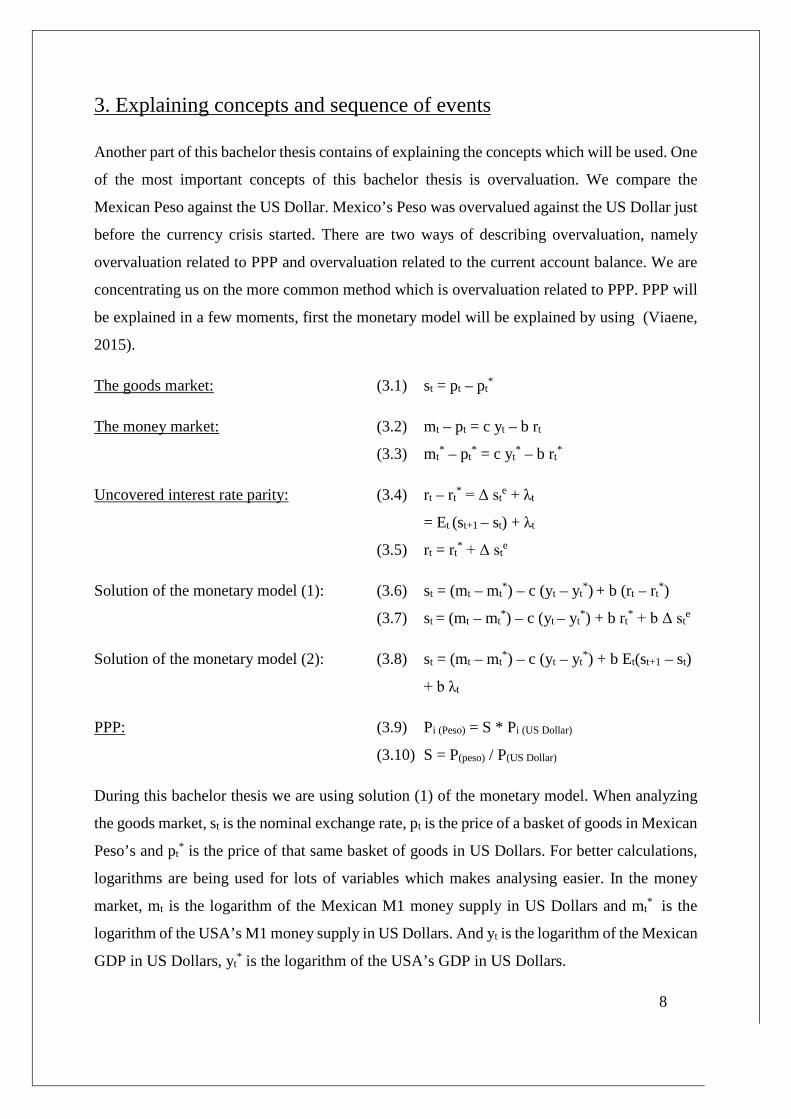
3. Explaining concepts and sequence of events

Another part of this bachelor thesis contains of explaining the concepts which will be used. One

of the most important concepts of this bachelor thesis is overvaluation. We compare the

Mexican Peso against the US Dollar. Mexico’s Peso was overvalued against the US Dollar just

before the currency crisis started. There are two ways of describing overvaluation, namely

overvaluation related to PPP and overvaluation related to the current account balance. We are

concentrating us on the more common method which is overvaluation related to PPP. PPP will

be explained in a few moments, first the monetary model will be explained by using (Viaene,

2015).

The goods market: (3.1) st = pt – pt*

The money market: (3.2) mt – pt = c yt – b rt

(3.3) mt* – pt

* = c yt* – b rt

*

Uncovered interest rate parity: (3.4) rt – rt* = Δ st

e + λt

= Et (st+1 – st) + λt

(3.5) rt = rt* + Δ st

e

Solution of the monetary model (1): (3.6) st = (mt – mt*) – c (yt – yt

*) + b (rt – rt*)

(3.7) st = (mt – mt*) – c (yt – yt

*) + b rt* + b Δ st

e

Solution of the monetary model (2): (3.8) st = (mt – mt*) – c (yt – yt

*) + b Et(st+1 – st)

+ b λt

PPP: (3.9) Pi (Peso) = S * Pi (US Dollar)

(3.10) S = P(peso) / P(US Dollar)

During this bachelor thesis we are using solution (1) of the monetary model. When analyzing

the goods market, st is the nominal exchange rate, pt is the price of a basket of goods in Mexican

Peso’s and pt* is the price of that same basket of goods in US Dollars. For better calculations,

logarithms are being used for lots of variables which makes analysing easier. In the money

market, mt is the logarithm of the Mexican M1 money supply in US Dollars and mt* is the

logarithm of the USA’s M1 money supply in US Dollars. And yt is the logarithm of the Mexican

GDP in US Dollars, yt* is the logarithm of the USA’s GDP in US Dollars.

8

Moreover, rt is the long term interest rate in Mexico and is noted in percentages and not in

logarithm. The same is assumed for rt* which is the USA’s long term interest rate. Continuing

our analysis, Δ ste is the expected depreciation of the Mexican Peso for the next period which

is nothing more as Et (st+1 – st), the expectation of the nominal exchange rate in Mexican Peso’s

per 1 US Dollar for the next period in the future minus the nominal exchange rate right now.

And λt is a disturbance term, it’s a constant term and has something to do with the political

differences of Mexico and the USA. This λt term will not be used during our analysis.

According to Copeland (2014), PPP (purchasing power parity) means that the price for a basket

of goods in Mexico must be equal to the price for that same basket of goods in the USA. One

extra variable is added here, the nominal exchange rate between the Mexican Peso and the US

Dollar. This nominal exchange rate S compensates the price differences between the two

currencies (see equation 3.8). Mexico is the home country and the USA is the foreign country.

S is equal to the Peso price level divided by the US Dollar price level (see equation 3.9). This

gives the PPP value of Peso’s in terms of US Dollars.

A higher S means a depreciation of the Peso related to the US Dollar and a lower S is an

appreciation of the Peso related to the US Dollar. Because this holds for every basket of goods

in the two countries, we can say that PPP holds for the general price level between in this case

Mexico and the USA. So P (MEX) = S * P (USA) (Copeland, 2014).

PPP says when converting two currencies into one common currency with their nominal

exchange rate, the price level must the same. Taking the logs of every term gives:

PPP: (3.11) p (MEX) = s * p (USA).

This means the absolute price and exchange rate levels are now replaced by relative price and

exchange rate changes (t1 – t0). dP (MEX) is the price difference for Mexico in Peso, dP (USA) is

the price difference for the USA in Dollars and dS is the nominal exchange rate difference

between the two time periods t1 and t0.

PPP: (3.12) dp (MEX) = dP (MEX) / P (MEX)

(3.13) dp (USA) = dP (USA) / P (USA)

(3.14) ds = dS / S

(3.15) dp (MEX) – dp (USA) = ds

9

Equation 3.14 says that Mexico’s inflation rate minus USA’s inflation rate is equal to the rate

of currency depreciation/appreciation (Copeland, 2014). According to PPP, inflation is very

determinative for calculating depreciation/appreciation.

In the case of Peso overvaluation, it means the actual spot exchange rate is higher as the PPP

exchange rate (Suranovic, 2006).

Overvaluation: (3.16) Pi (MEX) > S * Pi (USA)

This means PPP doesn’t hold anymore and the general price level in Mexico is relatively higher

as the general price level in the USA multiplied by the actual spot exchange rate (Suranovic,

2006). This means also that the actual nominal spot exchange rate is lower as the PPP nominal

spot exchange rate (see graph 2.1). Taking dp (MEX) – dp (USA) = ds, with overvaluation of the

Peso this formula becomes (3.17) dp (MEX) – dp (USA) > ds and

Overvaluation: (3.18) dp (MEX) > dp (USA) + ds.

This means the inflation rate in Mexico is bigger as the sum of the inflation rate in the USA

together with the appreciation of the Mexican Peso. So an American tourist in Mexico will

encounter that the actual price of a Mexican product is more than the PPP price (Suranovic,

2006). For Mexico, export becomes more expensive and import cheaper. Not only for tourists

the Mexican Peso is overvalued and too expensive, also for Mexican residents it becomes more

interesting to buy their products cheaper abroad (Suranovic, 2006). In the graph below we could

see the overvaluation of the Mexican Peso compared with the US Dollar in a graph. This

overvaluation started at the beginning of the nineties after a period of high economic growth in

Mexico. In the period between 1982 and 1985, the exchange rate system of Mexico was quite

fixed and controlled (Mexico, 2009), but this started to change in August 1985.

Graph 2.1: Overvaluation of the Mexican Peso in the years before the collapse of the fixed exchange rate system

Source: What-when-how, THE MEXICAN PESO CRISIS (FINANCE), http://what-when-how.com/finance/the-

mexican-peso-crisis-finance/ 10

In August 1985, Mexico’s exchange rate system changed and can be seen as an intermediate

fixed and floating system (Bordo, 2003). This means from August 1985, the controllable fixed

rate between the Peso and the US Dollar was still being used but could be modified regularly

by unequal amounts only if necessary (Banco of México). On a flexible way they tried to

maintain the fixed exchange rate as much as possible. For export benefits, Mexico decided in

November 1991 to introduce a new system which was quite synonymous to the old one. Right

now, a managed slippage exchange rate regime started to work which allowed the fixed

exchange rate to move within certain borders (Banco of México). These borders changed daily

and became widener, so that the chance of a border crossing was reduced. In this way the

financial authorities always kept control over the exchange rate. This is a so-called pegged

exchange rate system. Because of the Peso crisis the Mexican financial authorities couldn’t

sustain the crawling peg with the US Dollar and the pegged exchange rate system collapsed.

Right now every exchange rate upper/lower border disappeared (Banco of México). From this

point the free market decided in which direction the exchange rate moved, without monetary

interventions (van der Molen, 2013).

This brings us to the next important concept. In the first-generation model, the shadow exchange

rate (st*) is the exchange rate which is reached when the pegged exchange rate system changes

to a free-market floating system (Copeland, 2014). The shadow exchange rate will during this

bachelor thesis be indicated as st*. The actual exchange rate will be indicated as st.

In a pegged exchange rate system, the authorities always try to maintain a certain area in which

the exchange rate can move. But when they stop intervene, for example because the whole

system collapses due to an unexpected event, the exchange rate would automatically float to a

market-based exchange rate called the shadow exchange rate (Copeland, 2014). The shadow

exchange rate is based on the monetary model (Copeland, 2014). When the shadow exchange

rate and the fixed rate are equal to each other, we could say that temporarily no depreciation or

appreciation occurs if the system changes. With respect to this bachelor thesis, in words the

formula consists of the logs of the money stock relatively between Mexico and the USA, the

logs of real income relatively between Mexico and the USA and the interest rate differential

between Mexico and the USA. The shadow exchange rate formula is:

Shadow exchange rate: st* = (mt MEX – mt USA) – c (yt MEX – yt USA) + b (rt MEX – rt USA).

11

In this way we can calculate the shadow exchange rate using the monetary model. The collapse

of the pegged exchange rate system at December 22, 1994 has partially to do with the

prosperous years of Mexico before 1994. In 1993 and the beginning of 1994, Mexico had

economically the best period since a long time. The approval of NAFTA during the U.S.

Congress followed by reduced trade barriers between Mexico and the USA made Mexico

economically more wealthy. NAFTA is a free trade agreement between Canada, the USA and

Mexico and it stands for North American Free Trade Agreement. This agreement made Mexico

more attractive for domestic and foreign investors, mainly because Mexico was now more

accessible for American markets too. Therefore, Mexico benefited a lot from NAFTA (Whitt,

1996) and (Lustig and Fellow, 1995).

Mexico’s objectives were to decrease their budget deficit, reducing the inflation rate, abolishing

other trade barriers and the privatization of some government companies. The current account

deficit raised from six billion US dollars in 1989 to twenty billion US Dollars in 1992-1993.

Therefore, improving the huge current account deficit was a main objective for Mexico in 1993-

1994 (Whitt, 1996) and (Lustig and Fellow, 1995). Because of this large current account deficit,

the capital account had a big surplus.

This surplus could be a positive event, after all lots of capital amounts flew into the country and

international currency reserves rose. A current account deficit could be balanced by a capital

account surplus, at least in the short-term. The demand for Peso’s inclined as a result of a

increasing foreign demand for investing in Mexican capital and buying Mexican products.

Because of this capital surplus, a tendency to Peso appreciation started (Whitt, 1996) and

(Lustig and Fellow, 1995). Before this demand increase of the Mexican Peso, only a real

exchange rate depreciation of the Peso was expected. This is due to the fact that until then

Mexico had a pegged exchange rate system with a crawling peg where only the upper band

moved upwards periodically, meaning only a permission for a regularly nominal depreciation

of the Peso. But the opposite happened (Whitt, 1996) and (Lustig and Fellow, 1995). We speak

here about a real appreciation of the peso, where Q = SP*/P. Q is the real exchange rate, S is

the nominal exchange rate, P* is USA’s price level and P is Mexico’s price level. A higher Q

indicates a depreciation and a lower Q indicates an appreciation. In log terms, the real exchange

rate change is equal to the sum of the nominal exchange rate change and USA’s inflation rate

minus Mexico’s inflation rate.

12

Mexico’s inflation rate was in the early nineties very high. A smaller nominal depreciation of

the Peso or bigger inflation of the US Dollar was not enough to compensate the large Peso

inflation. Taking this into account, this indicates a real exchange rate appreciation according to

the theory. Because PPP couldn’t hold anymore, the Peso inclined to be overvalued related to

the US Dollar (Whitt, 1996) and (Lustig and Fellow, 1995). The combination of Peso’s

overvaluation and a huge capital account surplus made things slowly worse for Mexico. The

unexpected real exchange rate appreciation of the Peso made Mexican imports grow because

the American Dollar products became cheaper for Mexican residents, but conversely it reduced

the Mexican exports abroad. In this way this led to an even bigger current account deficit (Whitt,

1996) and (Lustig and Fellow, 1995).

But because of the economic instability which began to rose and the pegged exchange rate

system of Mexico with its fixed rate character, Mexico tried to maintain their currency value.

In order to undo the actual appreciation pressure, a short-term devaluation was needed. By

making arrangements between the government and the private sector to let the Peso devalue,

Mexico’s Central Bank thought everything was all right. The thought was that after this process

of devalue the Peso, where a short-term increase in prices was needed, in the long-term the

enormous inflation rate could go down. All this could lead to a short-term recession but to a

long-term stabilization of the economy. This long-term stabilization is because exports and

productivity would increase again in the long-term (Whitt, 1996) and (Lustig and Fellow, 1995).

To devalue their Peso, Mexico used their accumulated amount of international reserves as a

result of the surplus on the capital account. By selling their foreign currencies and buying Peso’s

The Mexican Central Bank tried to increase the supply of Peso’s in Mexico. By increasing the

supply of Peso’s together with a constant demand, the idea is that the Peso’s value decreases.

In this way a devaluation in a pegged exchange rate system was expected after a while. In this

way the Mexican government thought the economy would stabilize again. But they didn’t

thought about a devaluation as large as a collapse of the pegged exchange rate system (Whitt,

1996) and (Lustig and Fellow, 1995). As already said, in order to devalue the Peso international

foreign reserves were used. But at first Mexico hoped that only the capital account surplus could

lead to a future improved current account, without harming the international foreign reserves.

13

With the surplus of capital in Mexico, the government hoped that additional investments were

made in the form of new equipments and factories that would raise exports in the future.

In this way, the objective was to improve the current account using the capital inflows (Whitt,

1996) and (Lustig and Fellow, 1995). But in reality, the government underestimated the little

trust in the Peso of foreign investors and Mexican residents. Lots of investors removed their

capital and shares away from Mexico and exchanged it for other currency funds. They did this,

because speculations on the Peso were made and they expected a potential fall of the Peso. In

order to make profits in other trade markets before their capital devalues too, lots of investors

removed their capital away from Mexico and suddenly Mexico was not interesting for

investments anymore. This means there was a sudden and enormous decrease of capital inflows,

therefore the capital outflows and current account deficit couldn’t been compensated anymore

(Whitt, 1996; Lustig and Fellow, 1995).

From this moment, international foreign currencies were fully used to compensate the current

account deficit. But short-term inflation rose. In this way a non-stop current account deficit was

created, because exports continued to be relatively expensive and imports relatively cheap. The

capital outflow, together with a lower capital inflow, reduced the capital account and a rapidly

shrinkage of international reserves was inevitable. From this point, the international reserves

exhausted rapidly. In a short time there was a loss of almost 11 billion in international reserves

and the pressure on the Peso raised. An amount of reserves from almost 30 billion in February

1994 reduced to an amount of almost 5 billion in December 1994 (Whitt, 1996; Lustig and

Fellow, 1995). At this point the increased real interest rate through the Mexican Central Bank

in order to improve the capital account was a sign for the Mexican and foreign investors that

both capital and current accounts were difficult to keep balanced. The Mexican government

decided to devalue the Peso on 20 December 1994 as a result of a large economic instability

together with a rapid distrust in the Peso. This process was probably accelerated because

rumours of a possible exchange rate policy change made the speculations and distrust in the

Peso higher than ever (Whitt, 1996; Lustig and Fellow, 1995). Mexico devalued their Peso

almost 15% on the 20th December 1994. With a manual interference, where the upper band

rose, the Mexican government hoped the trust in the Peso would be restored and the economy

improved through domestic production and exports (Whitt, 1996; Lustig and Fellow, 1995).

14

But in reality the currency collapsed fully a few days after the announcement of the 15%

devaluation and a financial crisis was very close. One of the goals from the 15% devaluation

on December 22, 1994 was to stop the exhaustion of the foreign international reserves.

Another goal was to improve the accounts and reduce the outstanding foreign debts. A problem

here was that lots of Mexican debts were recognized as dollar debts, so-called debts that don’t

change in case of a Peso devaluation. Only defaulting on these foreign currency debts reduced

this US Dollar debt. But defaulting was not preferable, therefore this was hardly an option.

Although the devaluation of the Peso was set, a reduction of the US Dollar debts didn’t

occurred. US Dollar debts in Mexico are called Tesobonos.

On the other hand, the devaluation of the Peso made lots of foreign investors again shift their

funds away from Mexico. This arose because of a lack of trust in a fast recovery of the Mexican

Peso. While the Mexican government prepared their selves for a major capital outflow again, a

new option was created (Whitt, 1996; Lustig and Fellow, 1995). A dollar liquidity swap-line

with the USA could lead to improved market liquidity in which the demand for the Mexican

market was able to improve again. A dollar liquidity swap-line is an amount of credit funded

by the USA’s Fed to the Mexican Central Bank to improve liquidity problems in Mexico for

dollar markets. In this case, the USA helped Mexico and for the USA this meant they offered

dollars in foreign USA institutions for solving liquidity problems of Mexico. By doing this, a

swap-line of 7 billion US Dollars was created for Mexico on 22 December 1994 (Whitt, 1996;

Lustig and Fellow, 1995).

Another major announcement in 1994 on December, 22 was the collapse of the pegged

exchange rate system while a floating exchange rate system was introduced. After this

announcement, Mexico totally lost its worldwide, stable reputation. Moreover, the benefit of a

pegged exchange rate system for adjusting the real interest rate when necessary was lost. The

Peso collapsed even more now, the interest rates in Mexico rose a lot and the sale of Tesobonos

wasn’t by far as high as expected. But mainly the enormous reduction of the governments

influence to help Mexican markets had its impact. Depreciation of the Peso continued (Whitt,

1996; Lustig and Fellow, 1995).

15

4. Data and methodology

The content of this chapter contains of giving a precise description of the collected data and the

method which is used during the research on E-Views. Another part of this chapter is about

introducing and explaining the hypotheses.

The monetary model of the first generation model is used during the research. After the

assumption that the interest rate of Mexico is equal to the interest rate of the USA plus the

expected depreciation rate of the Mexican Peso, writing down this monetary model is as

follows: st* = (mt (mex) – mt (usa)) – c(yt (mex) – yt (usa)) + br*t + bΔse

t. In this overview, the shadow

exchange rate st* is very important. It’s a function of M1 money supply differentials and GDP

differentials, plus a long term nominal interest rate and expected rate of depreciation. The two

differentials containing the differences between Mexico’s and the USA’s numeric values of M1

money supply and GDP. The nominal interest rate is the foreign interest rate, the USA interest

rate. The expected rate of depreciation is calculated for the Mexican Peso. Putting everything

together we get a shadow exchange rate, the exchange rate which would be reached if a fixed

exchange rate system is replaced by a more floating exchange rate system (Copeland, 2014).

This is the monetary model.

The M1 money supply with currency and deposits (called m) and the GDP (called y) of Mexico

and the USA are both written in logarithms because analysis is easier and more valid by using

these terms instead of the huge numeric values. Because the interest rate of the USA (called r*t)

and the expected rate of Peso depreciation (called bΔset) are already in percentages, writing

down in logarithms isn’t needed over here. The interest rate of the USA is a long term nominal

interest rate, this rate was calculated of the ten year time of maturing for the US government

bonds. The expected rate of depreciation is zero for the period 1990Q1 till 1995Q1 during the

more fixed exchange rate regime. This is an obvious and clear assumption considering the fact

that we expect no change in the exchange rate for the next period during a fixed exchange rate

system where authorities try to maintain the current exchange rate as fixed as possible.

16

But after the collapse of this system and the introduction of a more flexible exchange rate,

matters change. Right now the expected rate of depreciation is calculated by another assumption

of the monetary model. This assumption says the expected rate of depreciation equals the

growth of domestic credit (Copeland, 2014). Since the M1 money supply after the fixed- rate

collapse contains mainly of domestic credit, the expected growth rate of domestic credit equals

the expected depreciation of the Mexican Peso (Copeland, 2014).

In formula: Δset+ = ΔMt+ , with the numeric values of M1 money supply from Mexico. Now we

can calculate the expected rate of depreciation using the M1 money supply. We do this by

calculating the growth rates of the numeric money supply values from Mexico. With these

growth rates, which is the growth of Mexico’s money supply in the current period compared

with the previous period, we obtain the expected depreciation/appreciation rates. The growth

rate of Mexico’s money supply in the current period is equal to the expected rate of

depreciation/appreciation of the Mexican Peso in the next period. A minus sign equals an

expected appreciation and a plus sign equals an expected depreciation.

All the data are on a quarterly basis from 1990Q1 till 2015Q2. Lots of data is founded on the

OECD database, this is a worldwide database with lots of historic economic data. The OECD

data of 1995Q2- 2015Q2 is used from every variable for deriving the coefficients, the OECD

data of 1990Q1-1995Q1 from every variable is used together with the coefficients for deriving

the shadow exchange rates. These shadow exchange rate results for the time interval 1990Q1-

1995Q1 are simulated results which will be explained later.

As already said, the regression is only for the period 1995Q1-2015Q2. By using the coefficients

of this analysis from every independent variable, we could calculate the answers for the period

1990Q1 till 1995Q1. However, there’s made one exception here for the regression model: for

the exchange rate s there’s data used for the whole time interval 1990Q1- 2015Q2. This is

because a comparison of the fixed nominal exchange rates during the period 1990Q1-1995Q1

and the simulated shadow exchange rates for period 1990Q1-1995Q1 is needed.

The regression equation used in E-Views is as follows:

s_d = β1 * lm1_diff_d – β2 * lgdp_diff_d + β3 * ir_usa_d + β4 * DUMDATE1 + β5 *

exp_deprec_d + resid. 17

DUMDATE1 needs some extra explanation. This is an extra variable added to the model. It’s

a dummy variable for the peak of the Global Financial crisis in 2009.

Originally this term isn’t part of the monetary model, but because of the huge residuals in 2008-

2010 this dummy is added extra to the model. It’s just a variable who indicates the impact of

the Global Financial Crisis. We give the value 1 during the period 2009Q1-2010Q1 (2009Q1,

2009Q2, 2009Q3, 2009Q4, 2010Q1) and 0 in all other periods and check what its coefficient is

and whether this coefficient is significant.

E-Views and Excel is used for making a backward simulation of the shadow exchange rate from

the monetary model for the period 1990Q1 till 1995Q1. OLS (ordinary least squares) is used as

the appropriate regression method. By using this regression method, the parameters and

significance of the linear regression are estimated. By making the regression on E-Views and

analysing the parameters and R-squared, four conditions are very important considering the

strength and validity of the OLS regression. These conditions which are tested and analysed

are:

• No autocorrelation for the error terms

• Homoscedasticity for the error terms

• Normal distribution for the error terms

• No perfect multicollinearity

In the next chapter there’s a description for every assumption, together with its results. Other

tests for checking the strength of the model are performed as well. By using the coefficients out

of the regression made on E-Views and the already known inserted data from every variable for

the period 1995Q1-2015Q2, we could simulate over the past. By calculating over the past with

Excel, we could simulate the shadow exchange rate for the period 1990Q1 till 1995Q1. After

modelling the simulation made on Excel, a comparison of the real rate with the shadow rate is

made for the period 1990Q1-1995Q1. We hope to find a point within the time interval 1990Q1-

1995Q1, where the actual exchange rates approximately equalize the simulated shadow

exchange rates. After analysing whether the collapse of the fixed exchange rate system was on

time according to the monetary model, we could make our conclusions.

Before we can say anything about actual results, hypotheses are relevant for statistical research.

They say something about expectations before results are available.

18 The first hypothesis says something about the timing of the collapse and is as follows: “H0: For the fixed exchange rate system in the period 1990Q1 till 1995Q1, the timing of the system change

according to the monetary model is approximately equal to the real time of system change”.

“Ha: For the fixed exchange rate system in the period 1990Q1 till 1995Q1, the timing of the system change

according to the monetary model is not at all equal to the real time of system change”.

With this hypothesis the representativeness of the monetary model will be tested. Was 1995Q1,

in which the exchange rate system changed, on time or were the monetary authorities of Mexico

too early or too late with introducing the floating system according to the monetary model? The

monetary model is tested based on a true event, so theory and practice are combined during this

research. We want to check whether the theory is significant enough for the practice and on

which scale the monetary model fits in this research. We expect that H0 will be maintained. In

other words, the timing of Mexican authorities for changing their policies regarding the

exchange rate system was on time according to the monetary model (Copeland, 2014).

The second hypothesis says something about the expected pattern of the shadow exchange rate

during the research range and is as follows: “H0: The patterns of the shadow exchange rate in the period 1990Q1 till 1995Q1 and 1995Q1 till 2015Q2

are linear”.

“Ha: The patterns of the shadow exchange rate in the period 1990Q1 till 1995Q1 and 1995Q1 till 2015Q2

are not linear”.

Here we check the linearity of the data. We check also if the patterns of the two time ranges

differ significantly from each other. In other words, is there a trend observable or is the pattern

of the data sets totally random? This means we check the patterns of the shadow exchange rate

for time interval 1990Q1 till 1995Q1 and for time interval 1995Q1 till 2015Q1. We expect

linearity by significance in both patterns.

The third hypothesis is about testing the coefficients of the single independent variables on its

own and is as follows: “H0: β1, β2, β3, β4, β5, β6 are together significant coefficients”

“Ha: β1, β2, β3, β4, β5, β6 are together no significant coefficients”

We check with this hypothesis the strength of the regression model, we expect the coefficients

together are significant and the coefficients are significantly different from zero.

19

5. Results In this chapter we will discuss the results of the research. We will talk about the results captured

from E-Views. The OLS assumptions and hypotheses are very important over here. The results

of E-Views with its OLS assumptions is the first paragraph of this chapter. The E-Views

regression output is as follows:

L = logarithm, DIFF = difference (Mexico-USA), IR = Nominal interest rate, M1 = M1 money supply,

EXP = Expected, DEPREC = Depreciation, GDP = Gross Domestic Product, DUMDATE1 = Dummy for

the Global Financial crisis in the period 2009Q1-2010Q1, D = First difference of the data (one lag).

Table 5.1: E-Views output

Table 5.2: Auto-correlation test (Breusch-Godfrey LM test with 1 lag to include)

F-statistic 58.51204 Prob. F(1,74) 0.0000

Obs*R-squared 35.76638 Prob. Chi-Square(1) 0.0000

20

Table 5.3: Heteroscedasticity test (Breusch-Pagan-Godfrey test)

F-statistic 1.095056 Prob. F(4,76) 0.3703

Variable Coefficient Standard

error

T-statistic Probability

C 24.49413 5.050059 4.850267 0.0000

LM1_DIFF_D 3.627645 0.443679 8.176282 0.0000

LGDP_DIFF_D 10.60503 5.535304 1.915890 0.0592

IR_USA_D -67.06225 8.713759 -7.696133 0.0000

DUMDATE1 1.351880 0.262045 5.158952 0.0000

EXP_DEPREC_D -0.342625 1.318037 -0.259951 0.7956

R2 0.933768 F-statistic 211.4771

Adjusted R2 0.929353 Prob(F-

statistic)

0.000000

Number of

observations after

one lag for every

leading variable

81

Obs*R-squared 5.510982 Prob. Chi-Square(4) 0.3567

Scaled Explained SS 5.168731 Prob. Chi-Square(4) 0.3956

Table 5.4: Normality test (Histogram Error terms with Jarque-Bera statistic)

Sample 1995Q2 2015Q2

Observations 81

Jarque-Bera 0.183650

Probability 0.912265

Graph 5.1: Output Normality test (Histogram Error terms with Jarque-Bera statistic)

Table 5.5: Multicollinearity test (VIF Factors)

Variable Coefficient Variance Uncentered VIF Centered VIF

C 25.50309 6951.479 NA

LM1_DIFF_D 0.196851 6.997574 3.340822

LGDP_DIFF_D 30.63959 7435.568 1.665618

IR_USA_D 75.92959 43.45900 4.338398

DUMDATE1 0.068668 1.155374 1.084055

EXP_DEPREC_D 1.737223 1.753997 1.038230

21 Table 5.6: Wald-test (Testing C1=C2=C3=C4=C5=C6)

Test statistic Value Df Probability F-statistic 6447.513 (5,75) 0.0000

0

1

2

3

4

5

6

7

8

9

-1.0 -0.5 0.0 0.5 1.0 1.5

Series: ResidualsSample 1995Q2 2015Q2Observations 81

Mean -2.06e-16Median 0.038375Maximum 1.570932Minimum -1.328133Std. Dev. 0.527820Skewness -0.069100Kurtosis 3.187925

Jarque-Bera 0.183650Probability 0.912265

Chi-Square 32237.57 5 0.0000

Table 5.7: Wald-test (Testing C1=C2=C3=C4=C5=C6=0)

In the first table of the regression output we find the data obtained from running the OLS

regression. Making all the data stationary is very important for using these data in regression

models. Every leading variable (so no C and no DUMDATE1) is made stationary by taking the

first difference (one lag) of the data from these variables. This is necessary because all these

variables have a unit root when we don’t use the first differences, in other words all these

variables are not stationary. By taking the first difference of every variable we obtain stationary

variables in which we reject the null-hypothesis of a unit root.

These stationary variables are appropriate for making and analyzing OLS-regressions. The _D

in the regression output stands for first difference and shows stationary variables. The C,

LM1_DIFF_D, IR_USA_D and DUMDATE1 are on its own significant variables where the

coefficients are very strong, also LGDP_DIFF_D is considered to be significant because its

probability is 0.0592 which is almost equal to the critical value of 0.05. For all these variables

the null-hypothesis of no significance is for at least 95% rejected according to these low values

of probability. Unfortunately EXP_DEPREC_D is not significant which means we cannot take

the values of these variable for certain, it’s the least reliable variable of the model. The R2 of

0.933768, which is the explanatory power of the model on the dependent variable S_D, is very

high. The regression model explains for more than 93% the dependant variable S_D. This

means the model fits very well. When we check four assumptions of OLS (ordinary least

squares), we cope with three of the four assumptions. Unfortunately there is some auto-

correlation of the error terms according to the Breusch-Godfrey LM test with one lag to include.

22

The low values of 0.0000 for the Prob. F(1,74) and Prob. Chi-Square(1) indicate a rejection of

the null-hypothesis for no auto-correlation. This means we have to accept the alternative

hypothesis which says there is some auto-correlation for the error term values within the dataset

Test statistic Value Df Probability

F-statistic 5373.653 (6,75) 0.0000

Chi-Square 32241.92 6 0.0000

of every independent variable. In other words, there is a to high degree of dependency for the

error terms of every single variable. Because randomness and independency are preferable, no

auto-correlation is a better feature. In a correlogram we find auto-correlation of the squared

error terms for the first obtained observations. In the chapter policy relevance and potential

improvements of this thesis, auto-correlation will be further discussed.

Fortunately the other assumptions of OLS we have tested are all satisfied. We obtain

homoscedasticity of the error terms, because the null-hypothesis from the Breusch-Pagan-

Godfrey test of homoscedasticity of the error terms is not rejected according to the value of

0.1630 which is more than the critical value 0.05. This means the variance of the error term is

significantly the same for all the independent variables and there’re no extreme outliers within

these variances. Therefore the scale of randomness is for every value of every independent

variable the same. This is very important by making regression models. Inserting the dummy

variable for the Global Financial Crisis is important for making the model homoscedastic.

We obtain also another very important assumption of OLS, which is the error terms are

normally distributed. According to the histogram we see a quite normal distribution of the error

terms. But with the help of the Jarque-Bera statistic 0.183650 and the Probability of 0.912265,

we could say the null-hypothesis of a normal distribution is by far not rejected. There’s a huge

certainty that the error terms of the independent variables have a significant normal distribution.

Also the assumption of no perfect multicollinearity is satisfied. The null-hypothesis of no

perfect multicollinearity is not rejected. All the Centered VIF values are below the critical value

of 5, so there is no perfect multicollinearity. If these values are higher than 5, multicollinearity

could be a problem which leads to incorrect data. No perfect multicollinearity means the leading

regressors are all linearly independent of each other which is preferable in a regression model.

With the Wald-test we test coefficient restrictions which are very important for analyzing the

model. C in E-Views is equivalently to β, this means C1=β1, C2=β2, C3=β3, C4=β4, C5=β5, C6=β6.

C1=C, C2=LM1_DIFF_D, C3=LGDP_DIFF_D, C4=IR_USA_D, C5=DUMDATE1,

C6=EXP_DEPREC_D.

23

When we test the hypothesis that every coefficient is significantly the same by

C1=C2=C3=C4=C5=C6 we find a rejection of the null-hypothesis that every coefficient is the

same. In other words, the coefficients are significantly different from each other. Also when we

test C1=C2=C3=C4=C5=C6=0 a rejection of the null-hypothesis is the case, therefore the

coefficients together are different from zero.

The date dummy variable has a positive impact on the fitness of the model. When making this

date dummy variable, we assumed after looking at a residuals graph for the whole time interval

with its outliers, the Global Financial Crisis had its biggest impact in 2009. That’s why the date

dummy variable is set on only 2009 plus the first quarter of 2010 for better model results.

Results are affected by the Global Financial Crisis, therefore we obtain a restriction in our

model in which we value the outcomes for the dependent variable higher during 2009 as in the

other years. The coefficient of 1.351880 for the DUMDATE1 means we add an extra value of

1.351880 * 1 = 1.351880 during 2009Q1-2010Q1. During the other periods this value is

1.351880 * 0 = 0. We could say, according to the model, the dummy for the Global Financial

Crisis has a positive effect of 1.351880 on the value of the exchange rate for the period 2009Q1-

2010Q1.

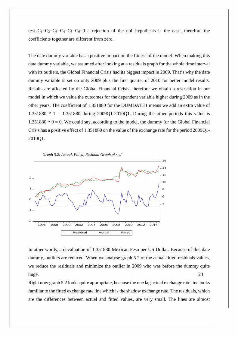
Graph 5.2: Actual, Fitted, Residual Graph of s_d

In other words, a devaluation of 1.351880 Mexican Peso per US Dollar. Because of this date

dummy, outliers are reduced. When we analyse graph 5.2 of the actual-fitted-residuals values,

we reduce the residuals and minimize the outlier in 2009 who was before the dummy quite

huge. 24

Right now graph 5.2 looks quite appropriate, because the one lag actual exchange rate line looks

familiar to the fitted exchange rate line which is the shadow exchange rate. The residuals, which

are the differences between actual and fitted values, are very small. The lines are almost

-2

-1

0

1

2

4

6

8

10

12

14

16

1996 1998 2000 2002 2004 2006 2008 2010 2012 2014

Residual Actual Fitted

identical. In other words, the actual rate and the calculated shadow exchange rate by E-Views

are almost identical for the period 1995Q1-2015Q1. The residuals are always around the zero-

line when we check graph 5.2. Small amounts of residuals of the dependent variable are

preferable, because in that way E-Views is able to regress the model optimally. For the period

1995Q1-2015Q1, E-Views is able to regress the model quite well. For the period 1990Q1-

1995Q1, we use another method which will be explained in a few moments.

When we check validity of the residuals, we observe just like every other variable stationary

residuals when we obtain the first differences of the residuals. Right now the null-hypothesis

of a unit root will be rejected and stationary residuals occurs. In table 5.8 the results are shown

if we take the first difference of the level values from the residuals.

Null- hypothesis: D(RESID) has a unit root. Exogenous: Constant. Lag length: 3 (Automatic-

based on SIC, maxlag=11) Table 5.8: Testing stationarity on the first differences of the residuals T-statistic Prob.

Augmented Dickey-Fuller test statistic -7.984902 0.0000

Test critical values: 1% level -3.521579

5% level -2.901217

10% level -2.587981

When analysing the other coefficients of the variables, we observe a depreciation of 3.627645

Mexican Peso’s per US Dollar when LM1_DIFF_D increases with one unit. An increase in

LM1_DIFF_D means a bigger increase in the logarithm of the M1 money supply of Mexico

compared with the logarithm of the M1 money supply of the USA. An increase in logarithm of

the M1 money supply is as an even higher increase in the absolute value of the M1 money

supply.

25

Ceteris paribus, when the logarithm of the one lagged M1 money supply differential (Mexico

– USA) increases by one unit, the Mexican Peso reduces in value for an amount equal to

3.627645 Mexican Peso’s per US Dollar. The only difference here is that the differentials of

the M1 money supply logarithms are negative instead of positive in our data, meaning a bigger

USA M1 money supply compared with Mexico’s M1 money supply. Knowing this, the

coefficient of 3.627645 has an appreciation effect on the shadow rate of the Mexican Peso per

US Dollar (s_d). The same analysis we could apply to LGDP_DIFF_D. Here an one unit

increase in LGDP_DIFF_D is equal to a depreciation of 10.60503 Mexican Peso’s per US

Dollar. In other words, an increase of the logarithm differential by one unit is equal to a

depreciation of the Mexican Peso for 10.60503 Mexican Peso’s per US Dollar. GDP has an

bigger effect on the exchange rate as M1 money supply, because 10.60503 is higher as

3.627645. In our data all the differentials of the GDP logarithms are again negative, meaning

the 10.60503 has an appreciation effect on the shadow rate of Mexican Peso per US Dollar

(s_d).

The coefficient of IR_USA_D has an appreciation effect on the shadow rate of the Mexican

Peso per US Dollar. The value of -67.06225 has to be analysed a little bit different because of

the interest rate scale in percentages. In our data, an interest rate increase of 0.01 (1% USA’s

nominal interest rate increase) combines a decrease of s_d (appreciation of the Mexican Peso

per US Dollar) for an amount of 0.6706225. The EXP_DEPREC_D has a counter effect on the

s_d, which is an unexpected result. But in this dataset, the effect of expected depreciation on

the shadow exchange rate is quite small. The value of -0.342625 says that an 1% (0.01) increase

in the expected rate of depreciation leads to a decrease of 0.00342625 of s_d, which is again

positive but this time a small appreciation effect on the Mexican Peso per US Dollar.

The next part is the analysis made on Excel for forecasting the shadow exchange rate. After this

process we could distinguish the shadow rates from the actual rates. Before showing the results,

an explanation is needed of how the results of the shadow rate are obtained. This shadow

exchange rate is the rate which would have been obtained if Mexican authorities stopped

intervening into the private markets to maintain the fixed rate. The shadow rate is the rate to

which the fixed rate immediately moves in case the exchange rate system changes from fixed

to flexible.

26 By making the regression on E-Views with the help of data of every variable found on World

Databanks, the right monetary model equation could be made. Adding the correct DUMMY

variable makes the model complete. After inserting all the data in E-Views on the right way

with lags, differences and logs, the output of the regression is important for analysis. Out of the

regression, the coefficients of every variable are used as beta’s for further calculations.

These coefficients are, together with the data of every variable, used for calculating the expected

exchange rate in Excel. For the whole time interval 1990Q1-2015Q2 these coefficients could

be used and in Excel there’s an option to vice these coefficients in an equation. By multiplying

these fixed coefficients with the data of all variables we get the shadow exchange rate. We don’t

insert the coefficient of the constant C in this equation because the monetary model is a

combination of M1 money supply, GDP, interest rates and expected depreciations and no

constant C is needed to insert here. This makes a more reliable prediction, moreover the results

of the shadow exchange rate are more close to the actual exchange rates. Both the actual

exchange rates from the OECD Stats Databank as the calculated shadow exchange rates are

derived for the period 1990Q1-2015Q2. The whole Excel sheet with all data and calculations

from 1990Q1-2015Q2 could be found in the appendix. But for now the most important time

intervals are the quarters before 1995Q1 and just after 1995Q1, because we expect our

conclusions could be made during this time interval which is around the actual collapse of the

pegged exchange rate system at 1994Q4.

The results of both exchange rates for 1990Q1-1996Q4 are inserted below. It’s the exchange

rate in Peso’s per US Dollar. During all quarters and in every expected exchange rate

calculation, the coefficients obtained from E-Views stay unchanged for every variable.

Conversely, the data of every variable is different for every quarter. We obtain calculations

from the shadow exchange rate and we add a lower and upper 10% boundary to the actual

exchange rate. This is done because the actual exchange rate is a measure in which some

movements are allowed. During most of this time interval, the present pegged exchange rate

system allowed some movements outside the actual rate and within some boundaries.

Therefore, 0.90 * st and 1.10 * st are obtained as well and we compare these data with the

calculated st* out of the data.

27 Table 5.9: The calculated shadow exchange rates versus the actual exchange rate

Time st* st 1.10 * st 0.90 * st

1990Q1 1-0.754658136 2.733 3.006 2.460

1990Q2 -0.867165288 2.820 3.102 2.538

1990Q3 -0.705865048 2.880 3.168 2.592

1990Q4 -0.344776422 2.930 3.223 2.637

1991Q1 -0.01264047 2.969 3.266 2.672

1991Q2 -0.111113845 3.006 3.307 2.705

1991Q3 0.887470147 3.044 3.348 2.740

1991Q4 1.384422089 3.070 3.377 2.763

1992Q1 1.404628675 3.065 3.372 2.759

1992Q2 1.353654152 3.098 3.408 2.788

1992Q3 1.902040279 3.097 3.407 2.787

1992Q4 1.953434181 3.120 3.432 2.808

1993Q1 2.216698743 3.105 3.416 2.795

1993Q2 2.462348943 3.115 3.427 2.804

1993Q3 2.675904983 3.116 3.428 2.804

1993Q4 2.867824399 3.126 3.439 2.813

1994Q1 2.450541983 3.177 3.495 2.859

1994Q2 1.776804371 3.343 3.677 3.009

1994Q3 1.592917827 3.395 3.735 3.056

1994Q4 1.232544498 3.640 4.004 3.276

1995Q1 1.573526242 6.007 6.608 5.406

1995Q2 6.01544 6.122 6.734 5.510

1995Q3 6.39937 6.215 6.837 5.594

1995Q4 6.75443 7.342 8.076 6.608

1996Q1 7.28468 7.522 8.274 6.770

1996Q2 7.47261 7.486 8.235 6.737

1996Q3 7.05374 7.559 8.315 6.803

1996Q4 7.17055 7.836 8.620 7.052

(OECD)

The result of -0.754658136 says that according to the monetary model and the data from

databanks, in 1990Q1 the expected exchange rate is 0.75 Mexican Peso’s (75 cents) equals 1

US Dollar. During this time interval 1990Q1-1996Q4 a certain depreciation of the shadow

exchange rate in Peso’s per US Dollar is observable. In other words, the value of the Mexican

Peso decreases compared with the US Dollar. Moreover, the actual exchange rates are

depreciating even faster as the shadow exchange rates.

28

1 The value of -0.754658136 is calculated as follows: S_D1990Q1 = 3.627645 * LM1_DIFF_D1990Q1 – 10.60503 * LGDP_DIFF_D1990Q1 – 67.06225 * IR_USA_D1990Q1 + 1.35188 * DUMDATE11990Q1 – 0.342625 * EXP_DEPREC_D1990Q1. For every quarter we use the same type of calculation but with different quarter data.

In table 5.9 we can see that for the shadow exchange rates the results for the period 1990Q1-

1995Q1 are obtained out of calculated backward simulations of the monetary model. For the

period 1995Q2-1996Q4, the results of the shadow exchange rates are equal to the fitted values

obtained from E-Views regression. The main objective of this research is to check whether

according to the monetary model the Mexican authorities reacted on the right time by changing

the exchange rate structure. We observe this by simulating the shadow exchange rate and adding

the actual exchange rate with 10% upper and lower boundaries. The actual exchange rates are

founded on the OECD Stats Worldbank website and are used for analysis. These actual rates

are the red, green and purple lines in graph 5.3 and these rates are in Peso’s per 1 US Dollar.

As already said, the shadow exchange rates are derived on another way. The shadow exchange

rate is the blue line in graph 5.3. These rates and partly backwards simulated and partly obtained

from E-Views results. For the period 1990Q1-1995Q1 (includes one lag), these shadow

exchange rates are calculated by backwards simulation of the monetary model. During this

period the data of every variable of the monetary model obtained from the OECD Stats

Worldbank is used for calculating the shadow exchange rates. For the period 1995Q2-2015Q2,

these shadow exchange rates are equal to the fitted values of the OLS regression on E-Views.

These calculated shadow exchange rates by E-Views are the expected rates of the actual rate

using the monetary model. In graph 5.3 we can see clear the patterns of the different exchange

rates for the period 1990Q1-2015Q2. The shadow exchange rate is st* and the actual exchange

rate is st. Graph 5.3: st

*, st, 1.10 * st and 0.90 * st for the period 1990Q1-2015Q2

29

st*

st

1.10 * st

0.90 * st

When the actual rate and the calculated shadow exchange rate intercept each other for the first

time, the first generation model of the monetary model says a pegged exchange rate system

would eventually collapse (Copeland, 2014). According to the monetary model, only if

authorities react at the point of interception by changing the system, a currency crisis could be

prevented. If authorities wait too long, overvaluation or undervaluation of the currency make

sure a currency system collapse and a financial crisis occurs.

In our research according to table 5.9 and graph 5.3, the shadow exchange rate and the actual

exchange rate are the closest to each other in late 1993, 1993Q4. When comparing the data, we

observe significantly the same values of the exchange rate in Peso’s per US Dollar at 1993Q4

for the st* and the 0.90 * st. During the fixed exchange rate system from 1990Q1-1995Q1, we

observe actual values around approximately 2.50 and 3.50 Peso’s per US Dollar. With an upper

and lower boundary of 10% in which the exchange rate could move, the lines intercept at

1993Q4. Especially the lower boundary of 0.90 * st intercepts the st* line very well in 1993Q4.

If Mexican authorities in the period 1990Q1-1995Q1 stopped intervening and let the exchange

rate free, the immediate result was appreciation towards the shadow exchange rate. At 1993Q4,

the interception of the 0.90 * st versus the st* means the Mexican government had to stop

intervening the fixed rate and had to move to the free rate where the market decides how the

exchange rate fluctuates. At this point it’s the best option to change the system from fixed to

more flexible. But Mexican authorities ignored this signal at 1993Q4 and didn’t change the

system at that time. After this a situation occurred in which the balance between the actual and

shadow rates disappeared more and more, followed by a massive loss of trust in the Mexican

Peso and a collapse of the pegged exchange rate system one year later in 1994Q4. Possibly, if

Mexican authorities reacted earlier, a currency crisis could have been prevented.

30

6. Policy relevance

Policy relevance matters too. We observe if and where the calculated expected exchange rate

(the shadow exchange rate) is approximately equal to the actual fixed rate. We could say

therefore that if the two rates are equal around 1994Q4, the monetary model succeeds in

explaining this exchange rate event. When the monetary model forecast an equality of both

rates on a certain point in time, authorities have to react on this according to the monetary model

by changing the structure. We could expect that if the authorities don’t react on this the crisis

occurs early or later no matter what. This is demonstrated in our research, where the monetary

model simulated a collapse around 1993Q4 but the collapse actually occurred a year later

around 1994Q4. Over time, this is considered to be a significant observation. Because the model

fits in general very well with all its tests and its explanatory power, the results are assumed to

be significant too.

Policy relevance in this sense is that the monetary model is doing a good job by backwards

simulating and explaining exchange rate crises. In other words, also in other cases where an

exchange rate collapse occurred the monetary model could help. Because in our research

simulating is backwards, forwards forecasting is difficult. But also by backwards simulating we

could check after an event occurred what the characteristics and patterns of the exchange rate

were according to the monetary model. By checking historic patterns of the shadow exchange

rate and the actual exchange rate on historic events, the monetary model could develop

warnings and learning points for future crises. Abnormal movements right now in money

supply, GDP, interest rates and/or expectations on currency depreciation could change the

shadow exchange rate between two currencies immediate and drastically.

In this way the monetary model could help predicting and preventing future exchange rate crises

right now by applying historic analysis of the monetary model out of different historic events.

Because the monetary model applying on the Mexican Peso crisis is just one analysis, more

analysis is needed for making the monetary model stronger. We could think about applying the

monetary model on more recent exchange rate crises where the currency is devaluating rapidly,

like the currencies in Russia and Argentina. The monetary model must play a role by central

banks and governments in order to react on abnormal movements and trying to prevent a

possibly future currency crisis.

31

7. Conclusions In the conclusions paragraph, answering the three hypotheses is very important. The first

hypothesis has something to do with the timing of the collapse. The first hypothesis is: “H0: For the fixed exchange rate system in the period 1990Q1 till 1995Q1, the timing of the system change

according to the monetary model is approximately equal to the real time of system change”.

“Ha: For the fixed exchange rate system in the period 1990Q1 till 1995Q1, the timing of the system change

according to the monetary model is not at all equal to the real time of system change”.

A “quiet” change at 1993Q4 was favourable where no appreciation or depreciation was

obtained if Mexican authorities changed their exchange rate system. Because Mexican

authorities waited too long, after 1993Q4 the mismatch became larger as we have seen and the

difference between the actual fixed rate and the shadow rate became bigger. After all we could

say the Mexican government reacted too late according to the monetary model. They reacted at

1994Q4, where according to the monetary model a reaction at 1993Q4 was favourable. Because

Mexico reacted to late, the Mexican Peso started to become overvalued after 1993Q4 and the

probability of a currency collapse rises. This is what actually happened and the Mexican Peso

collapsed at 1994Q4, a year later. If we link this information to the first hypothesis, we can say

the difference in timing of reaction was not very large but it also wasn’t exactly the same.

Therefore, we reject this null-hypothesis. We don’t have to reject the null-hypothesis for the

full 100%, but in general the timing isn’t totally equal. In other words, Mexican authorities

didn’t listen to the signals of the monetary model to change the currency system earlier.

The second hypothesis is: “H0: The patterns of the shadow exchange rate in the period 1990Q1 till 1995Q1 and 1995Q1 till 2015Q2

are linear”.

“Ha: The patterns of the shadow exchange rate in the period 1990Q1 till 1995Q1 and 1995Q1 till 2015Q2

are not linear”.

We could be short about this hypothesis. Fortunately, the pattern of the calculated shadow

exchange rate is perfectly linear during our total time interval 1990Q1-2015Q2. The only

exception here, in which there is no perfect linearity, is the small decrease of the st* line at 1993-

1994, just before the pegged exchange rate collapsed. But overall the st* line is linear.

32

A linear pattern is very important, because otherwise possibly no conclusions at all could have

been made about our research. If the pattern wouldn’t been linear, there was possibly no

interception at all between the shadow exchange rates and the actual rates. In this case no

interception means no system change is necessary at all. Another important implication is if the

shadow exchange rate pattern was completely based on randomness, no conclusions could have

been made related to the model and the monetary model would have been less reliable and less

valid. Randomness of the shadow exchange rate means no single signal of the monetary model

is significant because in the next period the shadow exchange rate could have been completely

different again. But fortunately we accept this null-hypothesis of linear patterns. In other words,

we can draw our conclusions based on the shadow exchange rate because it’s linear.

The third hypothesis is: “H0: β1, β2, β3, β4, β5, β6 are together significant coefficients”

“Ha: β1, β2, β3, β4, β5, β6 are together no significant coefficients”

This hypothesis is based on the Wald-test and the significance of the independent variables.

Fortunately, together the coefficients are significant and different from zero. The test

C1=C2=C3=C4=C5=C6=0 tests if all the independent variable coefficients together are

significantly different from zero or not. The null-hypothesis says the coefficients aren’t

significantly different from zero, the alternative hypothesis says they are different from zero.

This is an important test, because if these coefficients aren’t significantly different from zero it

means actually that all explanatory variables together don’t have any influence on the dependent

variable (the shadow exchange rate in Peso’s/Dollar). Fortunately the null-hypothesis of this

test is rejected when analyzing the probabilities, therefore the coefficients together are

significant and the coefficients all together are significantly different from zero. In other words,

the coefficients couldn’t be interpreted as significantly zero. Moreover, we could say with

certainty the coefficients tell us something about the relationship between the independent

variables and the dependent variable. Besides that, almost all single probabilities of the

explanatory variables are significant. Only EXP_DEPREC_D isn’t a significant variable. After

all, this null-hypothesis is accepted.

33

8. Shortcomings of the research

Shortcomings of the research are the limited amount of observations. Because the most

important data points are around 1993-1995 in which the conclusions are made, the availability

of a large data set is limited. We assume the monetary model is a good model while the model

is possibly not as good as assumed for our topic. Another shortcoming of the research is the

small influence of the expected depreciation on the shadow exchange rate, both the coefficient

and the data values. This variable is also insignificant which is another shortcoming. Another

shortcoming has something to do with the limited attention for other countries except Mexico

and the USA. We checked what happened with the Mexican Peso compared with the US Dollar

in which other currencies could have been used too.

For example a research with the Euro could have been made too. Besides that, we constantly

wrote only about the financial situation in Mexico. However, the collapse of the Mexican Peso

under a pegged exchange rate system had consequences for other countries like the USA too.

This could have been added to this bachelor thesis too, but will now be noted as a shortcoming.

Because it’s a large and international topic, there are always shortcomings. Lots of empirical

articles are written about this topic and many causes are mentioned, but no cause could have

been for the full 100% the reason. It’s always a combination of events. But according to the

research of this bachelor thesis, for future situations like this the monetary model could be taken

a little more serious.

34

9. References

Banco of México. Foreign Exchange Market (Exchange Rates). About Banco de México,

http://www.banxico.org.mx/portal-mercado-cambiario/foreign-exchange-markets--exc.html

[04-03-2015]

Bordo, M. D. (2003, August). Modern Exchange Rate Arrangements. IMF Working Paper:

Exchange Rate Regime Choice in Historical Perspective, https://www.imf.org/external/pubs

/ft/wp/2003/wp03160.pdf [11-06-2015]

Copeland, L. S. (2014). “Exchange Rates and International Finance sixth edition. Harlow:

Pearson Education Limited, 60-78, 150-161, 387-416.

Edwards, S. (1997, December). The Mexican Peso crisis: How much did we know? When did

we know it? NBER Working Paper Series, 1-10. http://www.nber.org/papers/w6334.pdf [08-

04-2016]

Eichengreen, B., Rose, A. K., & Wyplosz, C. (1994, October). Speculative attacks on pegged

exchange rates: an empirical exploration with special reference to the Euopean Monetary

system. National Bureau of Economic Research, 1-49. file:///C:/Users/Gebruiker/Pictures/

scriptie/w4898.pdf [10-2015]

Jr.A.Whitt, J. (1996, January/February). The Mexican Peso Crisis. Federal Reserve Bank of

Atlanta, 1-8. file:///C:/Users/Gebruiker/Downloads/Jwhi811%20(2).pdf [10-2015]

Lustig, N., & Fellow, S. (1995, June). The Mexican Peso crisis: the Foreseeable and the

Surprise. Brookings Institution, 2-5, 16-21. http://www.brookings.edu/views/papers/bdp/

bdp114/bdp114.pdf [09-2015]

Mathur, I., C.Gleason, K., & Singh, M. (1998, January 30). Did markets react efficiently to the

1994 Mexican peso crisis? Evidence from Mexican ADRS. Journal of Multinational Financial

Management (Elsevier), 40-42. http://down.cenet.org.cn/upfile/36/200541409251 87.pdf [06-

22-2015]

35

Mexico, B. D. (2009, September). Chronology of exchange rate regimes. Exchange Rate

Regimes in Mexico since 1954, 2-8. http://www.banxico.org.mx/sistema-financiero/material-

educativo/basico/%7BA363683E-9B8D-C3A9-610C-E2153395E4B8%7D.pdf [06-11-2015]

Mishkin, F. S. (1999, September 8th). Lessons from the Tequila Crisis; Policy lessons. Journal

of Banking and Finance (Sciencedirect), http://www.sciencedirect.com/science/

article/pii/S0378426699000291?np=y [09-2015]

OECD. Organisation for economic co-operation and development. OECD. Stat, http://stats.oecd.org/ [01-2016]

Suranovic, S. M. (2006, January 25th). Overvaluation and Undervaluation. International

Finance Theory and Policy, http://internationalecon.com/Finance/Fch30/F30-6.php [11-06-

2015]

The Economist. (2014, December 13). Pass the tequila. Mexico's economy, http://www.

economist.com/news/finance-and-economics/21636106-two-decades-after-peso-crisis-

mexico-faces-new-shocks-pass-tequila [06-22-2015]

Viaene, J.M. (2015, April 1th). Section 3.2 The 'news' models. Seminar: The Economics of Exchange Rates, http://bb-archive.eur.nl/bbcswebdav/pid-456407-dt-content-rid-32166831/ courses/FEB13037-14/FEB%2013037%20Slides%20Section%203.2.pdf [04-26-2016]

van der Molen, M. (2013, September 13th). The Tequila crisis in 1994. Economic Research,

file:///C:/Users/Gebruiker/Pictures/scriptie/The%20Tequila%20crisis%20in%201994%20-

%20Rabobank,%20Economic%20Research.html [11-06-2015]

36