anti-diffusive high order weno schemes for hamilton-jacobi...

METHODS AND APPLICATIONS OF ANALYSIS. c© 2005 International PressVol. 12, No. 2, pp. 169–190, June 2005 004

ANTI-DIFFUSIVE HIGH ORDER WENO SCHEMES FOR

HAMILTON-JACOBI EQUATIONS∗

ZHENGFU XU† AND CHI-WANG SHU‡

Dedicated to Professor Joel A. Smoller on the occasion of his 70th birthday

Abstract. In this paper, we generalize the technique of anti-diffusive flux corrections for highorder finite difference WENO schemes solving conservation laws in [21], to solve Hamilton-Jacobiequations. The objective is to obtain sharp resolution for kinks, which are derivative discontinuitiesin the viscosity solutions of Hamilton-Jacobi equations. We would like to resolve kinks better whilemaintaining high order accuracy in smooth regions. Numerical examples for one and two spacedimensional problems demonstrate the good quality of these Hamiltonian corrected WENO schemes.

Key words. Hamilton-Jacobi equations, anti-diffusive flux correction, kinks, Hamiltonian cor-rection, high order accuracy, finite difference, WENO scheme

AMS subject classifications. 65M06

1. Introduction. In this paper, we consider the numerical solutions of theHamilton-Jacobi equations

ut +H(ux1, · · · , uxn) = 0, u(x, 0) = u0(x). (1.1)

As is well known, solutions to (1.1) are Lipschitz continuous but could contain discon-tinuous derivatives, even when the initial conditions are smooth. Derivative disconti-nuities are observed as kinks in geometric structures. The nonuniqueness of solutionsto (1.1) also makes it necessary to define the concept of a viscosity solution, to singleout a unique, practically relevant solution. See Crandall and Lions [4].

In [5], Crandall and Lions proved convergence for first order monotone finite dif-ference schemes to the viscosity solutions of (1.1). To solve (1.1) with higher orderaccuracy, Osher and Sethian in [15] and Osher and Shu in [16] introduced a classof high order essentially non-oscillatory (ENO) schemes, which are adapted from themethodologies for hyperbolic conservation laws [7, 19, 20]. Weighted ENO (WENO)schemes for conservation laws [14, 10] are adapted to solve the Hamilton-Jacobi equa-tions in [9] for the rectangular meshes and in [22] for the triangular meshes. Runge-Kutta discontinuous Galerkin methods for conservation laws [3, 2] are also adaptedto solve the Hamilton-Jacobi equations in [8, 11, 13]. Numerical results producedby these high order schemes indicate convergence to the viscosity solutions of (1.1)with high order accuracy in smooth regions and sharp resolutions of the derivativediscontinuities.

We now concentrate on the issue of sharp resolutions of the derivative disconti-nuities, which is the main theme of this paper. High order finite difference WENOschemes for solving Hamilton-Jacobi equations [9] do produce better resolutions for

∗Received May 3, 2005; accepted for publication November 30, 2005. Research supported byARO grant W911NF-04-1-0291, NSF grants DMS-0207451 and DMS-0510345, and AFOSR grantFA9550-05-1-0123.

†Department of Mathematics, Pennsylvania State University, University Park, PA 16802, USA(xu [email protected]).

‡Division of Applied Mathematics, Brown University, Providence, Rhode Island 02912, USA([email protected]).

169

170 Z. XU AND C.-W. SHU

the derivative discontinuities than a low order scheme, especially for nonlinear prob-lems. However, for linear problems, numerical results by high order schemes stillsuffer from relatively poor resolutions of discontinuous derivatives comparing withthe resolution for nonlinear problems. This is a more serious issue for long time evo-lution, when the resolution of kinks becomes progressively worse. Considering theclose link between Hamilton-Jacobi equations and conservation laws, it is natural toadapt techniques of sharpening contact discontinuities for conservation laws to obtainsharper resolution of derivative discontinuities for Hamilton-Jacobi equations. In thispaper, we extend our work in [21] of anti-diffusive flux corrections for high order finitedifference WENO schemes for conservation laws to solve Hamilton-Jacobi equations.The technique we explored in [21] for sharpening contact discontinuities is adaptedto resolve derivative discontinuities for linear Hamilton-Jacobi equations both in onespace dimension and in two space dimensions.

This paper is organized as follows. In Section 2, we review briefly the anti-diffusive flux correction technique developed in [21], in a finite volume frameworkrather than in a finite difference framework as in [21]. This technique in a finitevolume framework for solving conservation law equations is then adapted to solveone dimensional Hamilton-Jacobi equations in Section 3. In Section 4, we generalizethis Hamiltonian correction method to two (or higher) dimensional Hamilton-Jacobiequations. We demonstrate the good numerical quality achieved by this Hamiltoniancorrection method through extensive numerical examples in Section 5. Concludingremarks are given in Section 6.

2. Flux corrections for high order finite volume WENO schemes. In thissection, we briefly review the flux correction technique developed and applied in [21]for solving conservation law equations both in one dimension and in two dimensions.However, instead of describing the technique in a finite difference framework as in[21], we present the technique in a finite volume framework which is easier to adaptto solve the Hamilton-Jacobi equations in next section.

2.1. Flux corrections for finite volume WENO schemes in one dimen-

sion. We consider the one dimensional conservation law

ut + f(u)x = 0 (2.1)

with f ′(u) > 0, for simplicity. The case with f ′(u) < 0 can be considered symmet-rically. We reintroduce the flux correction technique in [21] by a third order TVDRunge-Kutta method in time and a fifth order finite volume WENO discretization inspace, instead of the finite difference WENO discretization adopted in [21]. Noticethat the choice of fifth order WENO discretization in space and third order Runge-Kutta method in time is just for the convenience of presentation: the flux correctiontechnique can be applied to WENO schemes of any order and also to other Runge-Kutta methods. The full algorithm has the following form

u(1) = un + ∆tL(un)

u(2) = un +1

4∆tL(un) +

1

4∆tL(u(1)) (2.2)

un+1 = un +1

6∆tL(un) +

1

6∆tL(u(1)) +

2

3∆tL(u(2))

where u denotes the cell average of the solution u, ∆t is the time step which can bechanged from step to step, and L denotes the spatial WENO operator to be described

ANTI-DIFFUSIVE WENO SCHEMES FOR HAMILTON-JACOBI EQUATIONS 171

in detail below. In order to maintain the moving traveling wave solutions for piecewiseconstant functions containing contact discontinuities, we modified the scheme (2.2) in[21] by

u(1) = un + ∆tL(un)

u(2) = un +1

4∆tL′(un) +

1

4∆tL(u(1)) (2.3)

un+1 = un +1

6∆tL′′(un) +

1

6∆tL(u(1)) +

2

3∆tL(u(2))

where the operator L is defined by

L(u)i = −λi

(

fai+ 1

2− fa

i− 12

)

, (2.4)

with λi = ∆t∆xi

, where ∆xi is the local mesh size of cell i, and the anti-diffusive

numerical flux fa is given by

fa

i+ 12

= f�u−

i+ 12

�+ϕi minmod

�ui − ui−1

λi

+ f�u−

i− 12

�− f

�u−

i+ 12

�, f�u

+

i+ 12

�− f

�u−

i+ 12

��where u±

i+ 12

are the high order WENO reconstructions of the point values of u from

its cell averages u, with stencils biasing to the left and to the right respectively, see[10, 18] for details. The minmod function is defined as usual

minmod (a, b) =

0 a b ≤ 0

a a b > 0, |a| ≤ |b|b a b > 0, |a| > |b|

The operator L′ is defined by

L′

(u)i = −λi

(

fai+ 1

2− fa

i− 12

)

(2.5)

with the modified anti-diffusive flux fa given by

fa

i+ 12

=

8<:f

�u−

i+ 12

�+ ϕi minmod

�4(ui−ui−1)

λi+ f

�u−

i− 12

�− f

�u−

i+ 12

�, f

�u+

i+ 12

�− f

�u−

i+ 12

��fa

corresponding to the cases

{

b c > 0, |b| < |c|otherwise

(2.6)

respectively, and the operator L′′ is defined by

L′′(u)i = −λi

(

fai+ 1

2− fa

i− 12

)

(2.7)

with the modified anti-diffusive flux fa given by

fa

i+ 12

=

8<:f(u−

i+ 12

) + ϕi minmod�

6(ui−ui−1)

λi+ f

�u−

i− 12

�− f

�u−

i+ 12

�, f�u+

i+ 12

�− f

�u−

i+ 12

��fa


corresponding to the cases (2.6) respectively. Here b and c are defined as b = ui−ui−1

λi+

f(

u−i− 1

2

)

− f(

u−i+ 1

2

)

, c = f(

u+i+ 1

2

)

− f(

u−i+ 1

2

)

and ϕi is a discontinuity indicator

with its value between 0 and 1. Ideally, ϕi should be close to 0 in smooth regions andclose to 1 near a discontinuity. Our original choice of ϕi can be found in [21] and asomewhat improved choice is described in Section 2.2. We remark that the scheme(2.3) with L, L′ and L′′ defined by (2.4), (2.5) and (2.7) is fifth order accurate inspace and third order accurate in time. The correction to the original WENO scheme

is no larger in magnitude than that of f(

u+i+ 1

2

)

− f(

u−i+ 1

2

)

, which is on the level of

truncation errors for the WENO schemes because both u+i+ 1

2

and u−i+ 1

2

are high order

approximations to the same point value u(xi+ 12). This ensures that the high order

accuracy of the finite volume WENO schemes is achieved. The purpose of the extrafactor 4 in the first argument of the minmod function in the definition of fa and theextra factor 6 in the first argument of the minmod function in the definition of fa isto compensate for the coefficients 1

4 and 16 in front of L′ and L′′ respectively, so that

the final scheme could still maintain exactly traveling wave solutions of a piecewiseconstant function. We refer to [21] for more details.

For the upwind WENO-Roe schemes [10], the numerical flux is chosen as f(

u−i+ 1

2

)

when f ′(u) > 0 and as f(

u+i+ 1

2

)

when f ′(u) ≤ 0. The scheme described above is

therefore a flux corrected WENO-Roe scheme. Due to the entropy violating possi-bility of the Roe scheme, we only apply this technique on linear problems or linearlydegenerate fields of systems.

2.2. The discontinuity indicator. The discontinuity indicator ϕi is designedsuch that it is close to 0 in smooth regions and close to 1 near a discontinuity. Outof symmetry consideration and for the objective of a better description of the dis-continuity positions, we modify the definition of ϕi in [21] slightly to the followingform:

ϕi =βi

βi + γi

. (2.8)

with

αi = |ui−1 − ui|2 + ε, ξi = |ui−1 − ui+1|2 + ε, (2.9)

βi =ξi

αi−1+

ξi

αi+2, γi =

|umax − umin|2αi

.

Here ε is a small positive number taken as 10−6 in our numerical experiments, andumax and umin are the maximum and minimum values of uj for all cells. Clearly,0 ≤ ϕi ≤ 1, and ϕi = O(∆x2) in smooth regions. Near a strong discontinuity,γi ≪ βi, ϕi is close to 1.

2.3. Flux corrections for finite volume WENO schemes in two dimen-

sions. Two dimensional finite volume WENO schemes are similar to the schemes forone dimension described above, with reconstruction from two dimensional cell aver-ages to point values, which can be performed sequentially one dimension after anotherfor rectangular meshes. We refer to [17, 18] for more details. Thus, for example, af-ter the reconstruction of the point values ui+ 1

2 ,j and ui,j+ 12

at the interfaces, for theequation

ut + f(u)x + g(u)y = 0, f ′(u) > 0, g′(u) > 0,


we present the anti-diffusive flux by

fa

i+ 12

,j= f

�u−

i+ 12

,j

�+ ϕi,j minmod

�ui,j − ui−1,j

dλxi

+ f�u−

i− 12

,j

�− f

�u−

i+ 12

,j

�, f�u

+

i+ 12

,j

�− f

�u−

i+ 12

,j

��where d = 2 is the dimension. For fixed j, ϕi,j has the same definition as in (2.8) inone dimension. Symmetrically for the y direction, we have

ga

i,j+ 12

= g�u−

i,j+ 12

�+ ψi,j minmod

�ui,j − ui,j−1

d λyj

+ g�u−

i,j− 12

�− g

�u−

i,j+ 12

�, g�u

+

i,j+ 12

�− g

�u−

i,j+ 12

��with the discontinuity indicator ψi,j defined similarly to the one dimensional case in(2.8) in the y direction with fixed xi. The procedure described above applies to eachquadrature point along the cell interfaces to compute the numerical fluxes.

3. Hamiltonian corrected method for one dimensional Hamilton-Jacobi

equations. In this section, we consider the one dimensional Hamilton-Jacobi equa-tion

ut +H(ux) = 0 (3.1)

with H ′(u) > 0, for simplicity. The other case H ′(u) < 0 can be considered symmet-rically. The tight link between the Hamilton-Jacobi equation and the conservationlaw equation (2.1) in one dimension makes it easy to adapt schemes for conservationlaws to schemes for Hamilton-Jacobi equations [15]. We will adapt the flux correc-tion technique, developed in [21] and reviewed in the previous section, for sharpeningcontact discontinuities of high order WENO schemes for solving conservation laws,to sharpen kinks in the solutions of linear Hamilton-Jacobi equations. We start withthe adaptation of the first order scheme in [6] to the Hamilton-Jacobi equation.

3.1. First order Hamiltonian corrected method. We use the explicit form,interpreted in [1], of the limited down-wind scheme reintroduced in [6]. We referthe details of the limited down-wind scheme to [6]. Its simple explicit equivalentfinite volume scheme for the conservation law (2.1) with f ′(u) > 0 has the followingdefinition for the numerical flux

fai+ 1

2= f(ui) + minmod

(

ui − ui−1

λi

+ f(ui−1) − f(ui), f(ui+1) − f(ui)

)

. (3.2)

A relaxed version of (3.2) we have used is

fai+ 1

2= f(ui) + ϕi minmod

(

ui − ui−1

λi

+ f(ui−1) − f(ui), f(ui+1) − f(ui)

)

, (3.3)

where ϕi is the discontinuity indicator given by (2.8).This first order anti-diffusive scheme has the following property, which was proved

in [6, 1].

Proposition 3.1. Assume that the CFL condition λi f′(u) ≤ 1 holds, and the

numerical flux is defined by (3.3), then the scheme

un+1i − un

i + λi

(

fni+ 1

2− fn

i− 12

)

= 0 (3.4)


satisfies the maximum principle

minkun

k ≤ un+1i ≤ max

kun

k .

To solve the Hamilton-Jacobi equation (3.1), we define the first order divideddifference operator D− by

D−ui =ui − ui−1

∆x,

where ui = u(xi) is the point value of the solution u and for simplicity we assumethat the mesh size ∆x is a constant. This operator actually defines a cell average forux as it equals 1

∆x

∫ xi

xi−1ux dx. We adapt the finite volume scheme (3.4) and obtain

the following corrected numerical Hamiltonian

Hai = H(D−ui) (3.5)

+ ϕi minmod

�D−ui −D−ui−1

λi

+H(D−ui−1) −H(D−ui),H(D−ui+1) −H(D−ui)

�to form the following scheme

un+1i − un

i + ∆tHai = 0 (3.6)

for solving the Hamilton-Jacobi equation (3.1). Parallel to Proposition 3.1, we havethe following property for this first order Hamiltonian corrected scheme:

Proposition 3.2. Assume that the CFL condition λi H′(u) ≤ 1 holds, and

the numerical Hamiltonian is defined as in (3.5), then the scheme (3.6) satisfies themaximum principle for the first order divided difference

minkD−u

nk ≤ D−u

n+1i ≤ max

kD−u

nk . (3.7)

For the proof, we simply need to take the operator D− on (3.6) and then useProposition 3.1.

An immediate conclusion we can reach from Proposition 3.2 is

Proposition 3.3. Assume that the CFL condition λiH′(u) ≤ 1 holds, and the

numerical Hamiltonian is defined as in (3.5), then the scheme (3.6) is total variationbounded (TVB)

N∑

i=1

|uni − un

i−1| ≤ Lmaxi

|D−u0i | (3.8)

for any time level n, where L is the length of the domain for computation.


3.2. High order Hamiltonian corrected method. Using the first order di-vided differences D−ui and using the standard WENO procedure, we can reconstructD−

−ui and D+−ui as the left and right high order approximations of ux(xi). This

WENO reconstruction is given in details in [9]. We then adapt our anti-diffusive fifthorder finite volume WENO scheme, presented in Section 2, to the following Hamil-tonian corrected method for solving the Hamilton-Jacobi equation (3.1):

u(1) = un + ∆tL(un)

u(2) = un +1

4∆tL′(un) +

1

4∆tL(u(1)) (3.9)

un+1 = un +1

6∆tL′′(un) +

1

6∆tL(u(1)) +

2

3∆tL(u(2))

where the operator L is defined by

L(u)i = −Hai (3.10)

with the numerical Hamiltonian Ha given by

Hai = H(D−

−ui)

+ ϕi minmod

(

D−ui −D−ui−1

λi

+H(D−−ui−1) −H(D−

−ui), H(D+−ui) −H(D−

−ui)

)

The operator L′ is defined by

L′

(u)i = −Hai (3.11)


Hai =

(H(D−

−ui) + ϕi minmod

�4(D

−ui−D

−ui−1)

λi+ H(D−

−ui−1) − H(D−

−ui), H(D+

−ui) − H(D−

−ui)

�Ha

corresponding to the cases (2.6) respectively; the operator L′′ is defined by

L′′(u)i = −Hai (3.12)


Hai =

(H(D−

−ui) + ϕi minmod

�6(D

−ui−D

−ui−1)

λi+ H(D−

−ui−1) − H(D−

−ui), H(D+

−ui) − H(D−

−ui)

�Ha

corresponding to the cases (2.6) respectively, with b = D−ui−D−ui−1

λi+H(D−

−ui−1)−H(D−

−ui) and c = H(D+−ui) − H(D−

−ui). Finally, the kink indicator ϕi is againgiven by (2.8), with the cell averages u in (2.9) replaced by the first order divideddifferences D−u. This relaxation coefficient ϕi, which is a number between 0 and 1,is again introduced to give correction to the numerical Hamiltonians around kinks,and meanwhile to inherit the original WENO scheme in smooth regions.

Once again, we remark that the scheme (3.9) is fifth order accurate in space(when the WENO reconstruction is fifth order accurate) and third order accurate intime. The correction to the original WENO Hamiltonian is no larger in magnitudethan that of H(D+

−ui) −H(D−−ui), which is on the level of truncation errors for the

WENO schemes because both D+−ui and D−

−ui are high order approximations to the


point value ux at the same location xi. This guarantees that the high order accuracyof the WENO scheme is maintained. As before, the choice of fifth order WENOdiscretization in space and third order Runge-Kutta method in time is just for theconvenience of presentation: the Hamiltonian correction technique can be applied toWENO schemes of any order and also to other Runge-Kutta methods.

4. Hamiltonian corrected method for two dimensional Hamilton-Jacobi

equations. We have presented the flux corrected methods for high order finite dif-ference and finite volume WENO schemes for solving two dimensional conservationlaws in [21] and in Section 2, respectively. In this section, we directly adapt theanti-diffusive WENO schemes for two dimensional conservation law equations to twodimensional Hamilton-Jacobi equations

ut +H(x, y, ux, uy) = 0. (4.1)

For simplicity, we assume ∂H∂ux

> 0 and ∂H∂uy

> 0. Other cases can be treated symmet-

rically. Our Hamiltonian corrected scheme is given as follows

u(1) = un + ∆tL(un)

u(2) = un +1

4∆tL′(un) +

1

4∆tL(u(1)) (4.2)

un+1 = un +1

6∆tL′′(un) +

1

6∆tL(u(1)) +

2

3∆tL(u(2))

with the operator L(u) defined by

L(u)ij = −(Hi,j + Cxi,j + C

yi,j) (4.3)

where H is the upwind numerical Hamiltonian

Hi,j = H(xi, yj , D−x ui,j , D

−y ui,j),

andCxi,j andCy

i,j are the Hamiltonian corrections in the x and y directions respectively,defined by

Cxi,j = ϕi,j minmod

�Dxui,j −Dxui−1,j

d · λxi

+ Hi−1,j − Hi,j , H(xi, yj ,D+x ui,j ,D

−y ui,j) − Hi,j

�C

yi,j = ψi,j minmod

�Dyui,j −Dyui,j−1

d · λyj

+ Hi,j−1 − Hi,j ,H(xi, yj ,D−x ui,j ,D

+y ui,j) − Hi,j

�where d = 2 is the dimension. Same as in the one dimensional case, we fix j to defineDxui,j as

Dxui,j =ui,j − ui−1,j

∆xi

and symmetrically, we fix i to define Dyui,j as

Dyui,j =ui,j − ui,j−1

∆yj

.

We define the relaxation coefficients ϕi,j and ψi,j exactly the same way as in the onedimensional case in Section 3 by fixing j and i respectively. Finally, the modified


Table 5.1

Errors and numerical orders of accuracy of the fifth order Hamiltonian corrected fifth orderWENO scheme and the original fifth order WENO scheme for the one dimensional linear Hamilton-Jacobi equation (5.1).

Hamiltonian corrected WENO original WENON L1 error order L∞ error order L1 error order L∞ error order40 3.33E-6 5.34E-6 4.46E-5 7.72E-580 1.39E-6 4.58 2.20E-6 4.60 1.48E-6 4.91 2.41E-6 5.00160 4.66E-8 4.89 7.35E-8 4.78 4.73E-8 4.97 7.51E-8 5.00320 1.48E-9 4.97 2.34E-9 4.97 1.49E-9 4.99 2.35E-9 4.99640 4.66E-11 4.98 7.33E-11 4.99 4.66E-11 5.00 7.34E-11 5.00

operators L′ and L′′ can be defined similarly as before with the extra factors 4 and 6in the first arguments of the minmod functions respectively under the condition (2.6).

Again, this is a high order scheme according to the same observation that theHamiltonian correction is no larger in magnitude than the truncation error of theWENO reconstruction as in the one dimensional case. We will display numericaleffect of this scheme in next section, especially its quality in capturing kinks.

5. Numerical results. We give extensive numerical examples in this section todemonstrate the effect of the schemes we have developed in previous sections. Noticethat all PDEs in this section are understood to be the Hamilton-Jacobi equationsand we seek approximations to the viscosity solutions, which are continuous but maycontain discontinuous derivatives. The CFL number is taken as 0.3, except for theaccuracy tests where the CFL numbers are taken smaller for more refined meshes toguarantee that spatial errors dominate.

5.1. One dimensional problems. In this subsection we test our schemes onone dimensional scalar linear Hamilton-Jacobi equations. The computational domainis −1 < x ≤ 1 and periodic boundary conditions are used for all problems in thissubsection.

Example 5.1. We test the accuracy of the Hamiltonian corrected fifth orderWENO scheme for the linear Hamilton-Jacobi equation

ut + ux = 0 (5.1)

with the initial condition

u(x, 0) = sin(πx)

up to t = 2. The results and a comparison with the original fifth order WENO scheme[9] are given in Table 5.1. We can clearly see that fifth order accuracy is achieved andthe errors of the fifth order Hamiltonian corrected WENO scheme are comparablewith that of the original fifth order WENO scheme.

Example 5.2. We solve the linear Hamilton-Jacobi equation (5.1) with the initialcondition

u(x, 0) =

0, x ≤ −0.5

0.5− | x | | x |< 0.5

0 x > 0.5.

(5.2)


X

U

-1 -0.5 0 0.5 10

0.1

0.2

0.3

0.4

0.5

X

U

-1 -0.5 0 0.5 10

0.1

0.2

0.3

0.4

0.5

X

U

-1 -0.5 0 0.5 10

0.1

0.2

0.3

0.4

0.5

X

U

-1 -0.5 0 0.5 10

0.1

0.2

0.3

0.4

0.5

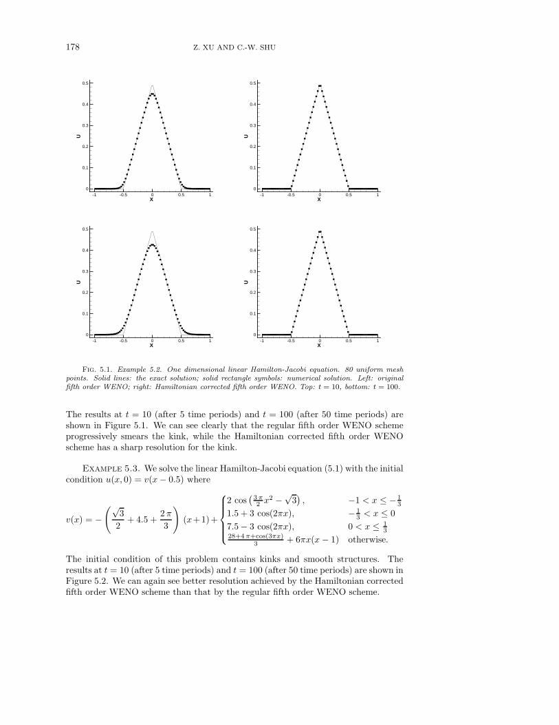
Fig. 5.1. Example 5.2. One dimensional linear Hamilton-Jacobi equation. 80 uniform meshpoints. Solid lines: the exact solution; solid rectangle symbols: numerical solution. Left: originalfifth order WENO; right: Hamiltonian corrected fifth order WENO. Top: t = 10, bottom: t = 100.

The results at t = 10 (after 5 time periods) and t = 100 (after 50 time periods) areshown in Figure 5.1. We can see clearly that the regular fifth order WENO schemeprogressively smears the kink, while the Hamiltonian corrected fifth order WENOscheme has a sharp resolution for the kink.

Example 5.3. We solve the linear Hamilton-Jacobi equation (5.1) with the initialcondition u(x, 0) = v(x− 0.5) where

v(x) = −(√

3

2+ 4.5 +

2 π

3

)

(x+1)+

2 cos(

3 π2 x

2 −√

3)

, −1 < x ≤ − 13

1.5 + 3 cos(2πx), − 13 < x ≤ 0

7.5 − 3 cos(2πx), 0 < x ≤ 13

28+4 π+cos(3πx)3 + 6πx(x − 1) otherwise.

The initial condition of this problem contains kinks and smooth structures. Theresults at t = 10 (after 5 time periods) and t = 100 (after 50 time periods) are shown inFigure 5.2. We can again see better resolution achieved by the Hamiltonian correctedfifth order WENO scheme than that by the regular fifth order WENO scheme.


X

U

-0.5 0 0.5-5.5

-5

-4.5

-4

-3.5

-3

-2.5

-2

-1.5

X

U

-0.5 0 0.5-5.5

-5

-4.5

-4

-3.5

-3

-2.5

-2

-1.5

X

U

-1 -0.5 0 0.5 1

-5

-4.5

-4

-3.5

-3

-2.5

-2

-1.5

-1

X

U

-1 -0.5 0 0.5 1

-5

-4.5

-4

-3.5

-3

-2.5

-2

-1.5

-1

Fig. 5.2. Example 5.3. One dimensional linear Hamilton-Jacobi equation. 200 uniform meshpoints. Solid lines: the exact solution; solid rectangle symbols: numerical solution. Left: originalfifth order WENO; right: Hamiltonian corrected fifth order WENO. Top: t = 10, bottom: t = 100.

5.2. Two dimensional problems. In this subsection we test our schemes ontwo dimensional linear Hamilton-Jacobi equations. The computational domain is(x, y) ∈ [−1, 1]2 with periodic boundary conditions.

Example 5.4. We solve the two dimensional linear Hamilton-Jacobi equation

ut + ux + uy = 0 (5.3)

with the initial condition given by:

u(x, y, 0) =

0, 0.7 ≤ r

0.7 − r, 0.2 < r < 0.7

0.5 r ≤ 0.2

with r =√

x2 + y2. The results at t = 2 (after 1 time period) and at t = 20 (after10 time periods) are given in Figures 5.3 and 5.4 for the one dimensional cuts and inFigure 5.5 for the two dimensional surfaces. We can observe a significant improvementof the Hamiltonian corrected fifth order WENO scheme over the regular fifth order


X

U

-1 -0.5 0 0.5 1

0

0.1

0.2

0.3

0.4

0.5

X

U

-1 -0.5 0 0.5 1

0

0.1

0.2

0.3

0.4

0.5

X

U

-1 -0.5 0 0.5 1

0

0.1

0.2

0.3

0.4

0.5

X

U

-1 -0.5 0 0.5 1

0

0.1

0.2

0.3

0.4

0.5

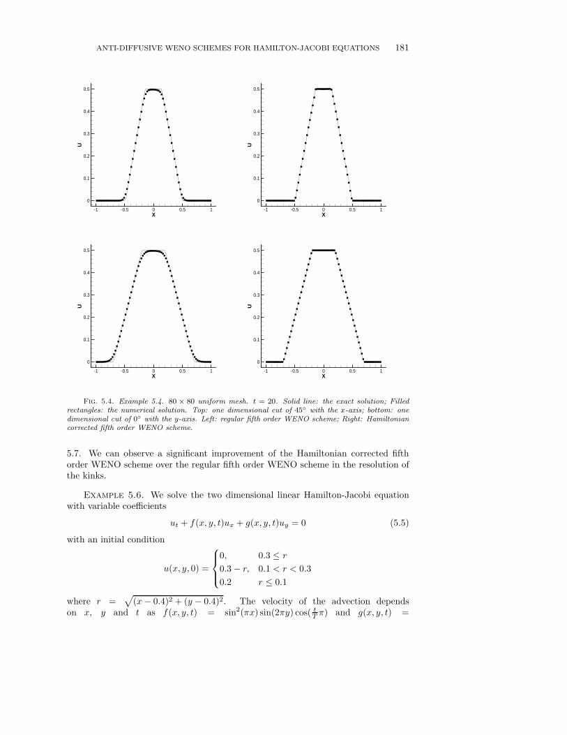
Fig. 5.3. Example 5.4. 80 × 80 uniform mesh. t = 2. Solid line: the exact solution; Filledrectangles: the numerical solution. Top: one dimensional cut of 45◦ with the x-axis; bottom: onedimensional cut of 0◦ with the y-axis. Left: regular fifth order WENO scheme; Right: Hamiltoniancorrected fifth order WENO scheme.

WENO scheme around the resolution of the kinks, especially for longer time. Thisimprovement can be seen most clearly in the zoomed surface plots in Figure 5.5.

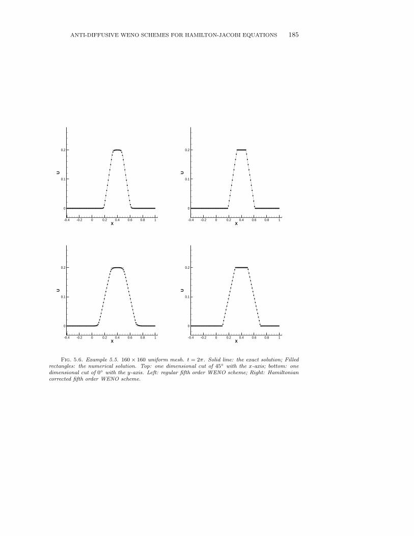
Example 5.5. We solve the two dimensional linear Hamilton-Jacobi equationwith variable coefficients

ut − yux + xuy = 0 (5.4)

with an initial condition

u(x, y, 0) =

0, 0.3 ≤ r

0.3 − r, 0.1 < r < 0.3

0.2 r ≤ 0.1

with r =√

(x− 0.4)2 + (y − 0.4)2. This is a solid body rotation around the origin.The computational result at t = 2π (after one rotation) is given in Figures 5.6 and


X

U

-1 -0.5 0 0.5 1

0

0.1

0.2

0.3

0.4

0.5

X

U

-1 -0.5 0 0.5 1

0

0.1

0.2

0.3

0.4

0.5

X

U

-1 -0.5 0 0.5 1

0

0.1

0.2

0.3

0.4

0.5

X

U

-1 -0.5 0 0.5 1

0

0.1

0.2

0.3

0.4

0.5

Fig. 5.4. Example 5.4. 80 × 80 uniform mesh. t = 20. Solid line: the exact solution; Filledrectangles: the numerical solution. Top: one dimensional cut of 45◦ with the x-axis; bottom: onedimensional cut of 0◦ with the y-axis. Left: regular fifth order WENO scheme; Right: Hamiltoniancorrected fifth order WENO scheme.

5.7. We can observe a significant improvement of the Hamiltonian corrected fifthorder WENO scheme over the regular fifth order WENO scheme in the resolution ofthe kinks.

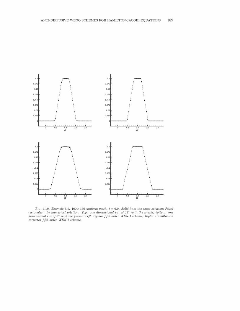
Example 5.6. We solve the two dimensional linear Hamilton-Jacobi equationwith variable coefficients

ut + f(x, y, t)ux + g(x, y, t)uy = 0 (5.5)

with an initial condition

u(x, y, 0) =

0, 0.3 ≤ r

0.3 − r, 0.1 < r < 0.3

0.2 r ≤ 0.1

where r =√

(x− 0.4)2 + (y − 0.4)2. The velocity of the advection dependson x, y and t as f(x, y, t) = sin2(πx) sin(2πy) cos( t

Tπ) and g(x, y, t) =


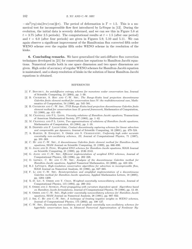
− sin2(πy) sin(2πx) cos( tTπ). The period of deformation is T = 1.5. This is a nu-

merical test for incompressible flow first introduced by LeVeque in [12]. During theevolution, the initial data is severely deformed, and we can see this in Figure 5.8 att = 3.75 (after 2.5 periods). The computational results at t = 1.5 (after one period)and t = 6.0 (after four periods) are given in Figures 5.9, 5.10 and 5.11. We canagain observe a significant improvement of the Hamiltonian flux corrected fifth orderWENO scheme over the regular fifth order WENO scheme in the resolution of thekinks.

6. Concluding remarks. We have generalized the anti-diffusive flux correctiontechniques developed in [21] for conservation law equations to Hamilton-Jacobi equa-tions. Numerical results both in one space dimension and two space dimensions aregiven. High order of accuracy of regular WENO schemes for Hamilton-Jacobi equationis maintained, and a sharp resolution of kinks in the solution of linear Hamilton-Jacobiequations is obtained.

REFERENCES

[1] F. Bouchut, An antidiffusive entropy scheme for monotone scalar conservation law, Journalof Scientific Computing, 21 (2004), pp. 1–30.

[2] B. Cockburn, S. Hou and C.-W. Shu, The Runge-Kutta local projection discontinuousGalerkin finite element method for conservation laws IV: the multidimensional case, Math-ematics of Computation, 54 (1990), pp. 545–581.

[3] B. Cockburn and C.-W. Shu, TVB Runge-Kutta local projection discontinuous Galerkin finiteelement method for conservation laws II: general framework, Mathematics of Computation,52 (1989), pp. 411–435.

[4] M. Crandall and P.L. Lions, Viscosity solutions of Hamilton-Jacobi equations, Transactionsof American Mathematical Society, 277 (1983), pp. 1–42.

[5] M. Crandall and P.L. Lions, Two approximations of solutions of Hamilton-Jacobi equations,Mathematics of Computation, 43 (1984), pp. 1–19.

[6] B. Despres and F. Lagoutiere, Contact discontinuity capturing schemes for linear advectionand compressible gas dynamics, Journal of Scientific Computing, 16 (2001), pp. 479–524.

[7] A. Harten, B. Engquist, S. Osher and S. Chakravathy, Uniformly high order accurateessentially non-oscillatory schemes, III, Journal of Computational Physics, 71 (1987),pp. 231–303.

[8] C. Hu and C.-W. Shu, A discontinuous Galerkin finite element method for Hamilton-Jacobiequations, SIAM Journal on Scientific Computing, 21 (1999), pp. 666–690.

[9] G. Jiang and D. Peng, Weighted ENO schemes for Hamilton-Jacobi equations, SIAM Journalon Scientific Computing, 21 (1999), pp. 2126–2143.

[10] G. Jiang and C.-W. Shu, Efficient implementation of weighted ENO schemes, Journal ofComputational Physics, 126 (1996), pp. 202–228.

[11] O. Lepsky, C. Hu and C.-W. Shu, Analysis of the discontinuous Galerkin method forHamilton-Jacobi equations, Applied Numerical Mathematics, 33 (2000), pp. 423–434.

[12] R.J. LeVeque, High-resolution conservative algorithms for advection in incompressible flow,SIAM Journal on Numerical Analysis, 33 (1996), pp. 627–665.

[13] F. Li and C.-W. Shu, Reinterpretation and simplified implementation of a discontinuousGalerkin method for Hamilton-Jacobi equations, Applied Mathematics Letters, 18 (2005),pp. 1204–1209.

[14] X.-D. Liu, S. Osher and T. Chan, Weighted essentially nonoscillatory schemes, Journal ofComputational Physics, 115 (1994), pp. 200–212.

[15] S. Osher and J. Sethian, Front propagating with curvature dependent speed: Algorithms basedon Hamilton-Jacobi formulations, Journal of Computational Physics, 79 (1988), pp. 12–49.

[16] S. Osher and C.-W. Shu, High-order essentially nonoscillatory schemes for Hamilton-Jacobiequations, SIAM Journal on Numerical Analysis, 28 (1991), pp. 907–922.

[17] J. Shi, C. Hu and C.-W. Shu, A technique of treating negative weights in WENO schemes,Journal of Computational Physics, 175 (2002), pp. 108–127.

[18] C.-W. Shu, Essentially non-oscillatory and weighted essentially non-oscillatory schemes forhyperbolic conservation laws, in Advanced Numerical Approximation of Nonlinear Hy-


perbolic Equations, B. Cockburn, C. Johnson, C.-W. Shu and E. Tadmor (Editor: A.Quarteroni), Lecture Notes in Mathematics, volume 1697, Springer, 1998, pp. 325–432.

[19] C.-W. Shu and S. Osher, Efficient implementation of essentially non-oscillatory shock-capturing schemes, Journal of Computational Physics, 77 (1988), pp. 439–471.

[20] C.-W. Shu and S. Osher, Efficient implementation of essentially non-oscillatory shock cap-turing schemes II, Journal of Computational Physics, 83 (1989), pp. 32–78.

[21] Z. Xu and C.-W. Shu, Anti-diffusive flux corrections for high order finite difference WENOschemes, Journal of Computational Physics, 205 (2005), pp. 458–485.

[22] Y.-T. Zhang and C.-W. Shu, High-order WENO schemes for Hamilton-Jacobi equations ontriangular meshes, SIAM Journal on Scientific Computing, 24 (2003), pp. 1005–1030.


Fig. 5.5. Example 5.4. Surface of 80 × 80 uniform mesh. t = 20. Top: the exact solution;middle: regular fifth order WENO; bottom: Hamiltonian corrected fifth order WENO. Left: full viewof the surface; Right: zoomed view of the angle with the x-y plane.


X

U

-0.4 -0.2 0 0.2 0.4 0.6 0.8 1

0

0.1

0.2

X

U

-0.4 -0.2 0 0.2 0.4 0.6 0.8 1

0

0.1

0.2

X

U

-0.4 -0.2 0 0.2 0.4 0.6 0.8 1

0

0.1

0.2

X

U

-0.4 -0.2 0 0.2 0.4 0.6 0.8 1

0

0.1

0.2

Fig. 5.6. Example 5.5. 160 × 160 uniform mesh. t = 2π. Solid line: the exact solution; Filledrectangles: the numerical solution. Top: one dimensional cut of 45◦ with the x-axis; bottom: onedimensional cut of 0◦ with the y-axis. Left: regular fifth order WENO scheme; Right: Hamiltoniancorrected fifth order WENO scheme.


-1

-1

-1Fig. 5.7. Example 5.5. Surface of 160 × 160 uniform mesh. t = 2π. Top: the exact solution;

middle: regular fifth order WENO; bottom: Hamiltonian corrected fifth order WENO. Left: full viewof the surface; Right: zoomed view of the angle with the x-y plane.


X

Y

0.5 1

0

0.25

0.5

0.75

1

X

Y

0.5 1

0

0.25

0.5

0.75

1

Fig. 5.8. Example 5.6. Contours at t = 3.75. Left: the regular fifth order WENO scheme;Right: Hamiltonian corrected fifth order WENO scheme.


X

U

0 0.2 0.4 0.6 0.8

0

0.025

0.05

0.075

0.1

0.125

0.15

0.175

0.2

X

U

0 0.2 0.4 0.6 0.8

0

0.025

0.05

0.075

0.1

0.125

0.15

0.175

0.2

X

U

0 0.2 0.4 0.6 0.8

0

0.025

0.05

0.075

0.1

0.125

0.15

0.175

0.2

X

U

0 0.2 0.4 0.6 0.8

0

0.025

0.05

0.075

0.1

0.125

0.15

0.175

0.2

Fig. 5.9. Example 5.6. 160 × 160 uniform mesh. t = 1.5. Solid line: the exact solution; Filledrectangles: the numerical solution. Top: one dimensional cut of 45◦ with the x-axis; bottom: onedimensional cut of 0◦ with the y-axis. Left: regular fifth order WENO scheme; Right: Hamiltoniancorrected fifth order WENO scheme.


X

U

0 0.2 0.4 0.6 0.8

0

0.025

0.05

0.075

0.1

0.125

0.15

0.175

0.2

X

U

0 0.2 0.4 0.6 0.8

0

0.025

0.05

0.075

0.1

0.125

0.15

0.175

0.2

X

U

0 0.2 0.4 0.6 0.8

0

0.025

0.05

0.075

0.1

0.125

0.15

0.175

0.2

X

U

0 0.2 0.4 0.6 0.8

0

0.025

0.05

0.075

0.1

0.125

0.15

0.175

0.2

Fig. 5.10. Example 5.6. 160×160 uniform mesh. t = 6.0. Solid line: the exact solution; Filledrectangles: the numerical solution. Top: one dimensional cut of 45◦ with the x-axis; bottom: onedimensional cut of 0◦ with the y-axis. Left: regular fifth order WENO scheme; Right: Hamiltoniancorrected fifth order WENO scheme.


Fig. 5.11. Example 5.6. Surface of 160 × 160 uniform mesh. t = 6.0. Top: the exact solution;middle: regular fifth order WENO; bottom: Hamiltonian corrected fifth order WENO. Left: full viewof the surface; Right: zoomed view of the angle with the x-y plane.

anti-diffusive high order weno schemes for hamilton-jacobi...

Documents