Anthropogenic climate change: what we know and don’t know

Steven SherwoodGeology and Geophysics Dept.

04/2004

Where did this “global warming” idea come from?

1) Early, obscure theoretical predictions (~1900)

2) Geologic evidence of large climate changes in the past--why, how?

3) Renewed modeling work (~1960+)

4) Late 20th-century warming that seems to stand above natural variability.

5) Really Bad Hollywood Movies

What we know for sure (and don’t…?)

1) CO2, CH4, N2O, halocarbs are IR absorbers and warm the surface: 2 x CO2 (from preindustrial) adds about 4 W m-2. But how much does T go up per W m-2?

2) CO2 rose 4%/decade since 1980, other gases rising too. But will this stay the same?

3) Global mean temperature rose by 0.6o C during 20th century. Many indirect indicators of warming (earlier spring blossomings and lake thaws, glacial retreat, melting permafrost, etc. etc.) But did we cause this?

4) Stratospheric temperatures are falling by ~ 1 C per decade. Due to GHG’s?

What we know for sure (and don’t…?)

1) CO2, CH4, N2O, halocarbs are IR absorbers and warm the surface: 2 x CO2 (from preindustrial) adds about 4 W m-2. But how much does T go up per W m-2?

2) CO2 rose 4%/decade since 1980, other gases rising too. But will this stay the same?

3) Global mean temperature rose by 0.6o C during 20th century. Many indirect indicators of warming (earlier spring blossomings and lake thaws, glacial retreat, melting permafrost, etc. etc.) But did we cause this?

4) Stratospheric temperatures are falling by ~ 1 C per decade. Due to GHG’s?

QuickTime™ and aTIFF (Uncompressed) decompressor

are needed to see this picture.

QuickTime™ and aTIFF (Uncompressed) decompressor

are needed to see this picture.

(NASA GISS)

What we know for sure (and don’t…?)

1) CO2, CH4, N2O, halocarbs are IR absorbers and warm the surface: 2 x CO2 (from preindustrial) adds about 4 W m-2. But how much does T go up per W m-2?

2) CO2 rose 4%/decade since 1980, other gases rising too. But will this stay the same?

3) Global mean temperature rose by 0.6o C during 20th century. Many indirect indicators of warming (earlier spring blossomings and lake thaws, glacial retreat, melting permafrost, etc. etc.) But did we cause this? Some, but not sure how much:• Regression analysis of last millennium• “GCM” simulations with/without “GHG’s” etc.• “Fingerprint analysis” of modern record

What we know for sure (and don’t…?)

1) CO2, CH4, N2O, halocarbs are IR absorbers and warm the surface: 2 x CO2 (from preindustrial) adds about 4 W m-2. But how much does T go up per W m-2?

2) CO2 rose 4%/decade since 1980, other gases rising too. But will this stay the same?

3) Global mean temperature rose by 0.6o C during 20th century. Many indirect indicators of warming (earlier spring blossomings and lake thaws, glacial retreat, melting permafrost, etc. etc.) But did we cause this?

4) Stratospheric temperatures are falling by ~ 1 C per decade. Due to GHG’s?

Yes, but O3 and H2O contribute strongly.

Stratospheric cooling by GHG’s2003

Water vapor changes are a key unknown.

What we want to know

• “Global warming” is only a first-order metric: we want regional variations, precipitation changes, glacial melt, extreme weather and other consequences!

• Alas, even the amount of future global warming is highly uncertain because of uncertainty in– Future CO2 levels,

– “Climate senstivity” dT/dln(CO2)

QuickTime™ and aTIFF (Uncompressed) decompressor

are needed to see this picture.

Y2000 US National Assessment: a tale of two models (neither from the US)

QuickTime™ and aTIFF (Uncompressed) decompressor

are needed to see this picture.

Climate sensitivity varies among GCM’s too.

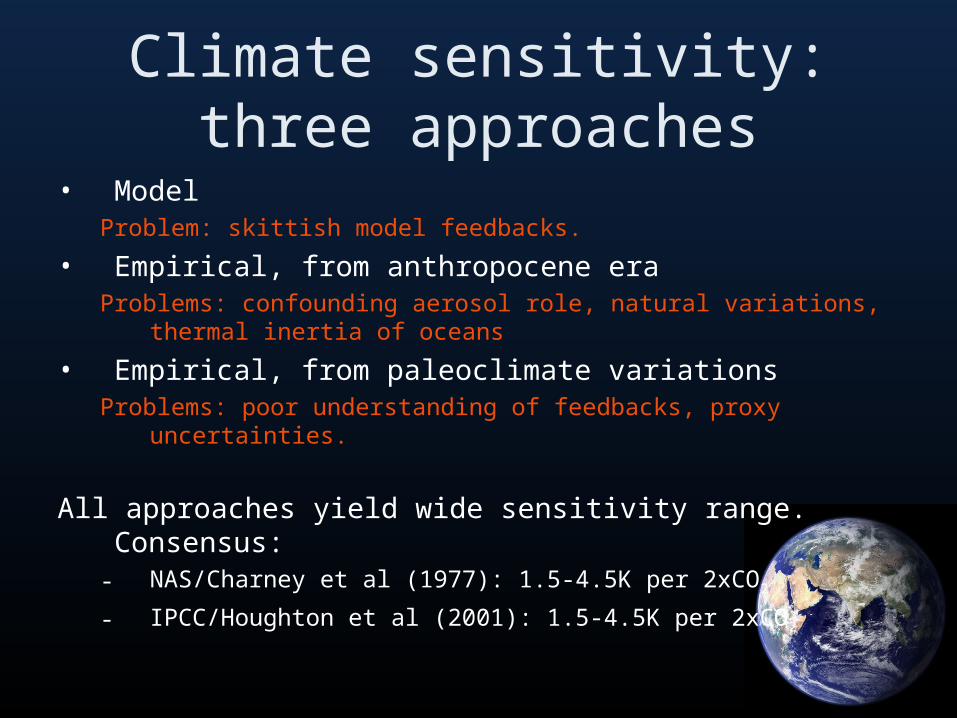
Climate sensitivity: three approaches

• ModelProblem: skittish model feedbacks.

• Empirical, from anthropocene eraProblems: confounding aerosol role, natural variations, thermal

inertia of oceans

• Empirical, from paleoclimate variationsProblems: poor understanding of feedbacks, proxy uncertainties.

All approaches yield wide sensitivity range. Consensus: - NAS/Charney et al (1977): 1.5-4.5K per 2xCO2

- IPCC/Houghton et al (2001): 1.5-4.5K per 2xCO2

Earth’s energy balance

Why is climate sensitivity so hard to quantify?

The solution, for a step change in forcing, is

€

σρc phdT

dt= δFforce

↓ −δFresponse↑

€

T(t) −Teq = δTe−t /τ

But h T/Fforce -- depends on the sensitivity!At equilibrium, for small perturbations we have

€

T = δFforce↓ /λ

λ ≡dFresponse

↑

dT=∂F↑

∂T+

∂F↑

∂qii

∑ dqidT

qi are variables (water vapor, cloud, ice) that affect F. With no feedbacks, 2xCO2 +1.2K.

3.8 Wm-2K-1

-1.5 (H2O)-1 (ice)? (clouds)

Water vapor feedback

• Clausius-Clapeyron relation implies saturation vapor pressure of H2O increases 6-17% per K; H2O strongest GHG!

• Actual H2O will presumably do same…?• The largest of the feedbacks, and most consistent

among models (roughly doubles sensitivity)• Lingering doubts about the possibility of universal model

failure? Microscale processes important? Relative humidity sensitive to T?

• Need either (a) full-physics model, or (b) a satisfying explanation for RH conservation.

Water vapor feedback

One possible heuristic explanation for RH conservation:1. Water vapor near saturation in small moist convective

regions;2. Water vapor mixing ratio conserved as air leaves;3. Dynamics maintains constant (small) difference

between temperatures in convective and elsewhere;4. Transport and horizontal organization of convective

regions don’t change muchHowever, one recent numerical experiment raises doubt

about constant-RH (Hartmann and Larson 2002).

QuickTime™ and aNone decompressor

are needed to see this picture.

Horizontal mixing rate

Mic

roph

ysic

al p

aram

eter

RH mean

RH range

Modeling of humidity distributions

Cloud feedback• Clouds reduce F by

infrared absorption, but increase F by solar reflection.

• Net effect is very sensitive to cloud altitude, water content, time of day, position.

• No simple rules for predicting these.

Cloud top altitude

• Height of upper-tropospheric clouds most important--produced by deep convective storms

• Storm height/intensity not well understood; may be controlled by– Buoyant instability of troposphere– Microphysical controls on cloud freezing/ease of raining– Airflow dynamics at “mesoscales”

• Thought to be regulated by position of tropopause

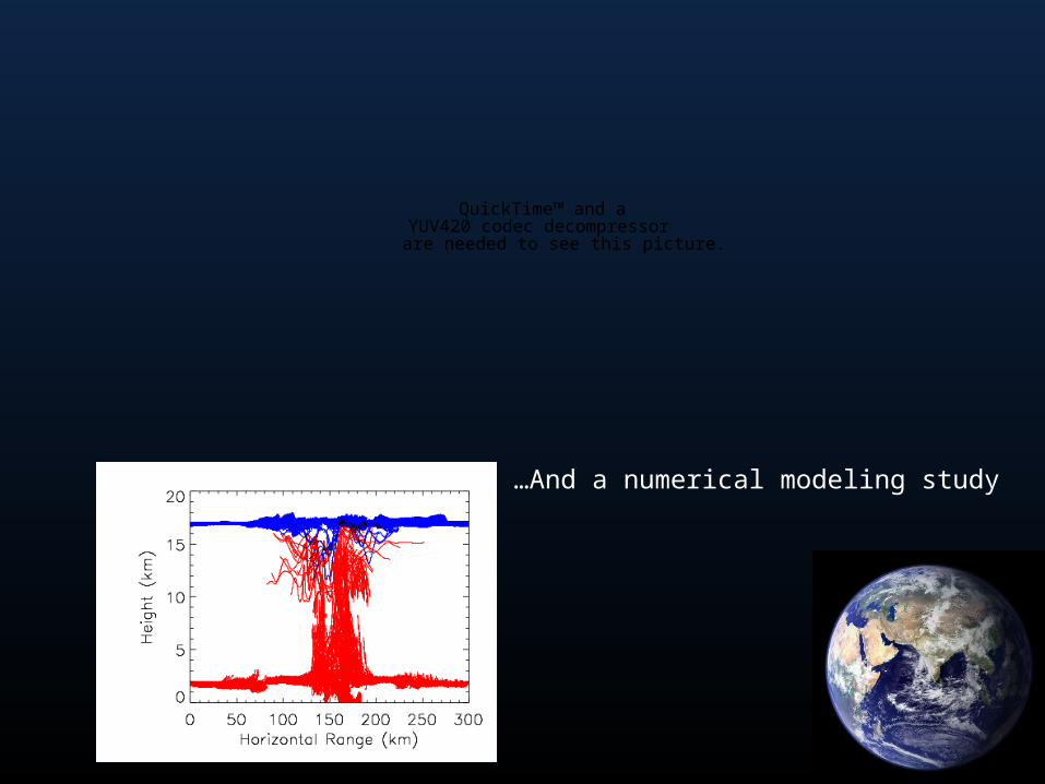
An observational study of the Florida region…

Deeper clouds over peninsula compared to surrounding oceans, as yet unexplained.

QuickTime™ and aYUV420 codec decompressor

are needed to see this picture.

…And a numerical modeling study

Cloud water content, area

• Some GCM’s assume water content proportional to saturation vapor pressure…raises …inconsistent with recent observations?

• Water content may be limited by ability of droplets to coalesce into raindrops

• If so, cloud water content and/or area should be increased by aerosols, but not T.

• Aerosols provide sites for cloud condensation -> ”indirect effect” -> current hot topic.

Detailed microphysical simulations

Clean environment

Polluted environment

Effect is apparent even in the tallest ice clouds, but tangled up with dynamics

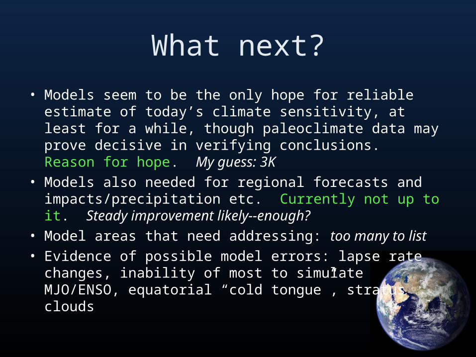
What next?

• Models seem to be the only hope for reliable estimate of today’s climate sensitivity, at least for a while, though paleoclimate data may prove decisive in verifying conclusions. Reason for hope. My guess: 3K

• Models also needed for regional forecasts and impacts/precipitation etc. Currently not up to it. Steady improvement likely--enough?

• Model areas that need addressing: too many to list• Evidence of possible model errors: lapse rate changes,

inability of most to simulate MJO/ENSO, equatorial “cold tongue”, stratus clouds

Summary

• “Climate sensitivity” is only the beginning, but is already quite difficult. Future GHG concentrations also hard to predict.

• GCM’s have many weaknesses and are nearly unfalsifiable, but still our main tool. Most available tests are only indirectly relevant to climate change.

• Human influence now widely accepted, based on many indirect analysis strategies.

• Yale G&G researchers are working on aerosol-cloud impacts, cloud greenhouse trapping, water vapor feedback, land and ecosystem hydrological interactions, ENSO and paleo-ENSO, all tied to the understanding of processes that determine climate sensitivity (and regional and hydrological behavior).

NCAR-GFDL difference due primarily to low cloud response difference

Allen and Ingram, 2002

Coupled AOGCM climate changes

1) Remote effects of tropical SST

Hoerling and Kumar 2003

Reasons for global influence of tropics

1) Isentropic surfaces

2) Diabatic overturning

3) Waves/PNA

Menon et al. 2002

2) Aerosol “direct effect”

SSA=0.85

SSA=1.00

JJA

JJA

Rosenfeld, 2000

Understanding the competition…

Larger (or more hydrophilic) particles are more appealing to water vapor molecules, hence activate sooner.

“Wal-Mart” effect:

more small

more large

Ocean-atmosphere influences

(NOAA)

1996

Warm surface -> clouds

but surface respondsto heat input

A really simple model of tropical air-sea interaction

€

dT

dt= −α 0T −α 1C + FT

C = βT + FC

T = Sea surface temperature anomalyC = Cloud cover anomalyFC, FT = stochastic forcings0,1, = positive constants (0.15, 0.5, 0.15)

Regression slope depends crucially on magnitudes of FT and FC!

Unpredictable atmosphere, obedient ocean(e.g. West Pacific Warm pool!)

Obedient atmosphere, unpredictable ocean(e.g. East equatorial Pacific)

Coupled OAGCM (NCAR PCM) simulation

Following Lindzen et al. 2001

Can feedbacks be “observed”?

• In this case, ocean-atmosphere interactions render the interpretation qualitatively sensitive to the underlying statistical model of the system.

• In general, previous attempts to observe feedbacks/sensitivity of poorly understood climate components do not appear to work.

• Other options are possible:

– fluctuation-dissipation– “fitted meta-parameterizations.”

Summary: what we know about variations of

• Global mean P

– climate warming ,– atmospheric absorbers .

• Regional P

– SST, absorbing aerosols (nonlocal dynamical) or , – CCN aerosols (local microphysical) or .

• Humidity

– CCN aerosols (local microphysical) in stratosphere,– Temperature effects? Don’t know yet, but significant

magnitude is increasingly doubtful (e.g. Pinatubo experiment, Soden et al 2002).

• Clouds, their role in global sensitivity

– not much (but low clouds probably more important).

“Global warming” climate sensitivity to CO2 etc.

• Original calculation (Ahrrenius 1896) within range of current uncertainty

• In GCM’s, main uncertainty is due to model differences in cloud cover response (sea ice also important)

– Cess 1989: factor of three uncertainty among models (most crude by today’s standards)

– Cess 1996: range narrowed significantly as sophistication increases

– 2003: more “improvements”; range broadening again?• Key problem: no theory for cloud cover or cloud properties.

2003 Model intercomparison

QuickTime™ and aYUV420 codec decompressorare needed to see this picture.

Infrared emission Solar albedo