Ant Colony Optimization and Its Application tothe Vehicle Routing Problem with Pickups andDeliveries

Bulent Catay

Abstract. Ant Colony Optimization (ACO) is a population-based metaheuristic thatcan be used to find approximate solutions to difficult optimization problems. It wasfirst introduced for solving the Traveling Salesperson Problem. Since then manyimplementations of ACO have been proposed for a variety of combinatorial opti-mization problems. In this chapter, ACO is applied to the Vehicle Routing Problemwith Pickups and Deliveries (VRPPD). VRPPD determines a set of vehicle routesoriginating and ending at a single depot and visiting all customers exactly once. Thevehicles are not only required to deliver goods but also to pick up some goods fromthe customers. The objective is to minimize the total distance traversed. The chapterfirst provides an overview of the ACO approach. Next, VRPPD is described and therelated literature is reviewed. Then, an ACO approach for VRPPD is presented. Theapproach proposes a new visibility function which attempts to capture the “deliv-ery” and “pickup” nature of the problem. The performance of the approach is testedusing well-known benchmark problems from the literature.

1 Introduction

Ant Colony Optimization (ACO) is a population-based metaheuristic that can beused to find approximate solutions to difficult optimization problems [16]. It wasfirst introduced for solving the Traveling Salesperson Problem (TSP) [15, 18]. Sincethen many implementations of ACO have been proposed for a variety of combina-torial optimization problems such as Quadratic Assignment Problem [34], Schedul-ing Problems [11], Sequential Ordering Problem [21], and various Vehicle RoutingProblems [5, 6, 14, 22, 30, 31].

The approach is based on the observation of the behavior of real ant coloniessearching for food sources. Real ants deposit an aromatic essence, called pheromone,

Bulent CataySabanci University, Faculty of Engineering and Natural Sciences,Tuzla, 34956 Istanbul, Turkeye-mail: catay@sabanciuniv.edu

on the path they walk. Other ants searching for food sense that pheromone and usethis information in selecting their path. The quantity of pheromone deposited on apath is based on the length of the path and the quality of the food source. As moreants follow a path the level of pheromone on that path will increase, thus increasingits selection probability by other ants. In ACO, artificial ants are used for searchinggood solutions to an optimization problem by taking advantage of this cooperativelearning process.

In this chapter, we apply the ACO approach to the well-known Vehicle Rout-ing Problem with Pickups and Deliveries (VRPPD). The classical Vehicle RoutingProblem (VRP) involves a set of delivery customers to be serviced by a fleet of ve-hicles housed at a central depot. The objective of the problem is to develop a set ofvehicle routes originating and terminating at the depot such that all customers areserviced, the demands of the customers assigned to each route do not violate thecapacity of the vehicle that services the route, and the total distance traveled by allvehicles is minimized. VRPPD is a variant of the VRP where the vehicles are notonly required to deliver goods to customers but also to pick up some goods fromthe customers. Customers receiving goods are called linehauls and customers send-ing goods are called backhauls. VRPPD may be classified into three categories: (i)Deliveries First, Pickups Second: the vehicles pick up goods only after they havedelivered their goods; (ii) Mixed Pickups and Deliveries: the vehicles deliver andpick up goods in any sequence along their routes; and (iii) Simultaneous Pickupsand Deliveries: the vehicles simultaneously deliver and pick up goods [28].

VRP with delivery first, pickup second is the first VRPPD problem introduced inthe literature and is known as the VRP with Backhauls (VRPB). The reason why thevehicles have to finish delivering their load before they start picking up items maybe due to the difficulty of rearranging the delivery and pickup items on the vehicles,e.g. rear loaded vehicles. However, it is also possible to perform both tasks in anyorder or simultaneously when the vehicle is nearly empty or is designed for bothrear and side loading and unloading. Hence, several variants of this problem havebeen proposed over time relaxing the restriction of servicing backhaul customersafter the linehauls as well as introducing multiple-depot cases. In this chapter, weconsider two of these variants: Mixed VRP with Backhauls (MVRPB) and VRPwith Simultaneous Pickups and Deliveries (VRPSPD). In MVRPB and VRPSPDthe objective and constraints are the same as in VRPB except the servicing order ofthe customers, which makes the former two problems more complicated because ofthe fluctuating loads on the vehicle along the route.

VRPB has been extensively studied in the literature. However, the research onMVRPB is scant and VRPSPD has only recently received some attention. Thesetwo problems are more realistic and applicable to real-world situations. This chapterattacks these problems using an ant algorithm and is organized as follows: Section 2depicts the mechanism of the ACO metaheuristic and summarizes some of the vari-ants proposed in the literature. Section 3 is devoted to the description of VRPPDand the overview of various approaches proposed for solving the problem. Section4 introduces an ACO approach by proposing a new visibility function and Section 5

presents the computational experiments and numerical results. Finally, concludingremarks are given in the last section.

2 Ant Colony Optimization

ACO is a metaheuristic approach designed for solving hard combinatorial optimiza-tion problems. Real ant colonies deposit pheromone on the paths they walk whilesearching for food sources. If other ants searching for food sense the pheromone ona path, they are likely to follow it rather than traveling at random, thus reinforcingthe path. As more and more ants follow a path the level of pheromone on that pathwill enhance, which in turn will increase its selection probability by other ants. Onthe other hand, the pheromone evaporates over time, reducing the chance of otherants following the path. The longer the path between the nest and the food sourcethe more the pheromone evaporates. Thus, the pheromone levels remain higher onthe shorter paths. As a consequence, the level of pheromone laid is basically basedon the path length and the quality of the food source.

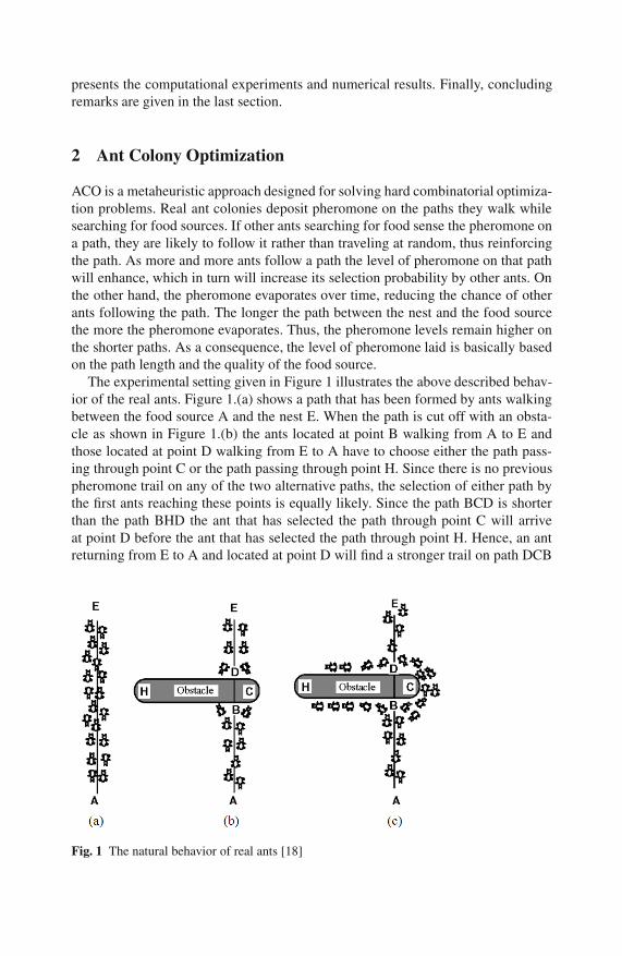
The experimental setting given in Figure 1 illustrates the above described behav-ior of the real ants. Figure 1.(a) shows a path that has been formed by ants walkingbetween the food source A and the nest E. When the path is cut off with an obsta-cle as shown in Figure 1.(b) the ants located at point B walking from A to E andthose located at point D walking from E to A have to choose either the path pass-ing through point C or the path passing through point H. Since there is no previouspheromone trail on any of the two alternative paths, the selection of either path bythe first ants reaching these points is equally likely. Since the path BCD is shorterthan the path BHD the ant that has selected the path through point C will arriveat point D before the ant that has selected the path through point H. Hence, an antreturning from E to A and located at point D will find a stronger trail on path DCB

Fig. 1 The natural behavior of real ants [18]

due to the ants that have already selected that path by chance and those walkingthrough BCD. Therefore, the selection probability of path DCB will be larger thanthat of path DHB. Consequently, the amount of pheromone on path BCD will in-crease faster than the pheromone on path BHD because of the larger number of antsfollowing path BCD per unit time and the evaporation factor. In time, all ants willselect the shorter path [18].

ACO simulates this natural behavior of real ants to solve combinatorial optimiza-tion problems by using artificial ants. To apply ACO, the optimization problem istransformed into the problem of finding the best path on a weighted graph. Theartificial ants incrementally build solutions by moving on the graph using a stochas-tic construction process guided by artificial pheromone and heuristic informationknown as visibility [16]. The amount of pheromone deposited on arcs is propor-tional to the quality of the solution generated and increases at run-time during thecomputation.

The Ant System (AS) is the first ACO algorithm which was applied for solvingthe TSP [15, 18]. Given a number of cities and the costs of traveling from any cityto any other city, TSP aims at finding the least-cost round-trip route that visits eachcity exactly once and then returns to the starting city. In AS, each ant probabilisti-cally chooses the next city to visit based on a heuristic combining the distance tothat city and the amount of virtual pheromone deposited on the arc to that city. Theants explore, depositing pheromone on each arc they cross, until they have all com-pleted a tour. At this point the ant which has completed the shortest tour depositsvirtual pheromone along its complete tour. The amount of pheromone deposited isinversely proportional to the tour length; i.e., the shorter the tour, the more amountof pheromone the ant deposits on the arcs of the corresponding tour.

Although AS provided competitive results its performance was still inferior inlarge instances compared to other algorithms specifically designed for the TSP [19].However, its successful application has led to many extensions for various combi-natorial optimization problems utilizing a similar construction mechanism. Someearly applications include the elitist strategy for Ant System (EAS) [15, 18], rank-based version of Ant System (ASrank) [6], MAX-MIN Ant System (MMAS) [35],Ant Colony System (ACS) [17], and Multiple Ant Colony System (MACS) [22].

In the next section we provide a more detailed explanation of the mechanisms ofAS approach and its extensions applied to the TSP.

2.1 Ant System

In AS , K artificial ants probabilistically construct tours in parallel exploiting a givenpheromone model. Initially, all ants are placed on randomly chosen cities. At eachiteration, each ant moves from one city to another, keeping track of the partial solu-tion it has constructed so far. The algorithm has two fundamental components:

• The amount of pheromone on arc (i, j), τi j

• Desirability of arc (i, j), ηi j

where arc (i, j) denotes the connection between city i and city j.

At the start of the algorithm an initial amount of pheromone τ0 is deposited oneach arc: τi j = τ0 = K/L0, where L0 is the length of an initial feasible tour and K isthe number of ants. In AS, the initial tour is constructed using the nearest-neighboralgorithm; however, another TSP heuristic may be utilized as well. The desirabilityvalue (also referred to as visibility or heuristic information) between a pair of citiesis the inverse of their distance ηi j = 1/di j, where di j is the distance between citiesi and j. So, if the distance on the arc (i, j) is long, visiting city j after city i (orvice-versa) will be less desirable.

Each ant constructs its own tour utilizing a transition probability: an ant k posi-tioned at a city i selects the next city j to visit with a probability given by

pki j =

⎧⎪⎪⎨

⎪⎪⎩

ταi j ηβ

i j

∑l∈Nk

i

ταil ηβ

il

, if j ∈ Nki

0 , otherwise

(1)

Here, Nki denotes the set of not yet visited cities; α and β are positive parameters to

control the relative weight of pheromone information τi j and heuristic information

ηi j. Note that ταi j η

βi j is also referred to as the attractiveness and is denoted as ϕi j.

After each ant has completed its tour, the pheromone levels are updated. Thepheromone update consists of the pheromone evaporation and pheromone reinforce-ment. The pheromone evaporation refers to uniformly decreasing the pheromonevalues on all arcs. The aim is to prevent the rapid convergence of the algorithm toa local optimal solution by reducing the probability of repeatedly selecting certaincities. The pheromone reinforcement process, on the other hand, allows each ant todeposit a certain amount of pheromone on the arcs belonging to its tour. The aimis to increase the probability of selecting the arcs frequently used by the ants thatconstruct short tours. The pheromone update rule is the following:

τi j ← (1−ρ)τi j +K

∑k=1

Δτki j, ∀(i, j) (2)

In this formulation, ρ (0 < ρ ≤ 1) is the pheromone evaporation parameter andΔτk

i j is the amount of pheromone deposited on arc (i, j) by ant k and is computed asfollows:

Δτki j =

{1Lk , if ant k uses arc (i, j) on its tour

0 , otherwise(3)

where Lk is the length of tour constructed by ant k.Prior to the pheromone update a local search procedure may be applied on the

tours constructed by the ants to reduce the distance traversed. It has been observedthat such a procedure enhances the performance of the AS algorithm. In Figure 2 anoverview of the steps of the algorithm is provided.

Fig. 2 Description of AS

2.2 The Extensions of AS

In the EAS [15, 18] an elitist strategy is implemented by further increasing thepheromone levels on the arcs belonging to the best tour achieved since the initiationof the algorithm. That best-so-far tour is referred to as the “global-best” tour. Thepheromone update rule is as follows:

τi j ← (1−ρ)τi j +K

∑k=1

Δτki j + wΔτgb

i j , ∀(i, j) (4)

Here, w denotes the weight associated with the global-best tour and Δτgbi j is the

amount of pheromone deposited on arc (i, j) by the global-best ant and calculatedby the following formula:

Δτgbi j =

{1

Lgb , if global best ant uses arc (i, j) on its tour

0 , otherwise(5)

where Lgb is the length of global-best tour.In the ASrank [6] a rank-based elitist strategy is adopted in an attempt to pre-

vent the algorithm from being trapped in a local minimum. In this strategy, w best-ranked ants are used to update the pheromone levels and the amount of pheromonedeposited by each ant decreases with its rank. Furthermore, at each iteration, theglobal-best ant is allowed to deposit the largest amount of pheromone. The updaterule is the following:

τi j ← (1−ρ)τi j +w−1

∑r=1

(w− r)Δτri j + wΔτgb

i j , ∀(i, j) (6)

The ACS presented in [17] attempts to improve AS by increasing the impor-tance of exploitation versus exploration of the search space. This is achieved by

employing a strong elitist strategy to update pheromone levels and a pseudo-randomproportional rule in selecting the next node to visit. The strong elitist strategy isapplied by using the global-best ant only to increase the pheromone levels on thearcs that belong to the global-best tour:

τi j ← (1−ρ)τi j + ρΔτgbi j , ∀(i, j) (7)

The mechanism of the pseudo-random proportional rule is as follows: an ant k lo-cated at customer i may either visit its most favorable customer or randomly selecta customer. The selection rule is the following:

jk =

⎧⎨

⎩

argmaxj∈Nk

i

ταi j η

βi j , if z≤ z0

Jk , otherwise(8)

where z is a random variable drawn from a uniform distribution U[0,1] and z0 (0≤ z0 ≤ 1) is a parameter to control exploitation versus exploration. Jk is selected ac-cording to the probability distribution (1). ACS also uses local pheromone updatingwhile building solutions: as soon as an ant moves from city i to city j the pheromonelevel on arc (i, j) is reduced in an attempt to promote the exploration of other arcsby other ants. The local pheromone update is performed as follows:

τi j← (1− ξ )τi j + ξ τ0 (9)

where ξ is a positive parameter less than 1.Similar to ACS, MMAS [35] uses either the global-best ant or the iteration-best

ant alone to reinforce the pheromone. It has been observed that using iteration-best ant at the start of the algorithm and then gradually increasing the frequencyof using the global-best ant for the pheromone update improves the performance.However, this strategy may cause a rapid convergence to a sub-optimal solution.Thus, maximum and minimum limits on the pheromone levels are imposed to avoidstagnation. The interval in which the pheromone may vary is set to [τmin, τmax]. Thepheromone levels are initialized at τmax to allow the exploration of the search spaceat the beginning. In addition, the pheromone levels are reinitialized whenever thesystem approaches stagnation or no improvement has been achieved after a numberof consecutive iterations.

Gambardella et al. [22] developed a multiple ACS (MACS) for solving the VRPwith Time Windows (VRPTW). VRPTW has two objectives: to minimize the num-ber of vehicles used and the total tour time. The former is considered to be the pri-mary objective, i.e. a solution with less number of vehicles but longer travel time ispreferred over a solution with more vehicles but shorter travel time. MACS attemptsto minimize both objectives simultaneously by using two parallel ant colonies. Thefirst colony, named as ACS-VEI, reduces the number of vehicles while the second,named as ACS-TIME, minimizes the total tour time by using the number of vehicles

provided by ACS-VEI. Although the two ant colonies run in parallel they use inde-pendent pheromone trails.

The interested reader is referred to [19] for more details on ACO metaheuristicand its variants.

3 Vehicle Routing Problem with Pickups and Deliveries

In this section, we first describe VRPPD and present a 0-1 mixed integer linearprogramming model following the formulation of [13]. We next review the existingliterature on MVRPB and VRPSPD.

3.1 Problem Description

VRPPD deals with a single depot distribution/collection system servicing a set ofcustomers by means of a homogeneous fleet of vehicles, i.e. all vehicles have thesame capacity. The customers may require two types of service: a delivery and/ora pickup. Products to be delivered are loaded at the depot and products picked upare transported back to the depot. The objective is to find the set of vehicle routesservicing all the customers with the minimum total distance. A maximum routelength restriction may be imposed on the vehicles.

In VRPB, each customer has either a delivery or a pickup demand to be satisfiedand the vehicle services the linehaul customers first. The main reasoning behindvisiting linehaul customers before backhaul customers is the fact that linehaul cus-tomers have precedence over backhaul customers in many real world cases and ve-hicles are often rear loaded. The latter causes problems when rearranging the itemson the vehicle, thus preventing the mixed routes and simultaneous pickup and de-livery. However, the improved design of vehicles allows side loadings, making themixed routes a more practical option since that would provide shorter routes. Thus,in MVRPB, each customer has either a delivery or a pickup demand and backhauland linehaul customers may be visited in any order. On the other hand, servicingthe customers in any order but not allowing simultaneous pickup and delivery isnot practical and realistic in many real world situations. As a result, VRPSPD wasproposed where each customer has both a delivery and a pickup demand and bothservices are performed simultaneously. Although the customers can be visited inany order along the route in both problems they must be serviced exactly once.

From a practical point of view VRPPD models situations such as distribution ofbottled drinks, chemicals, LPG tanks, laundry service of hotels, etc. where the cus-tomers are typically visited for a double service. In the case of the distribution of thebottled drinks for instance, full bottles are delivered to customers and empty ones arebrought back either for re-use or for recycling. In the distribution of chemicals case,some hazardous materials may need to be returned for safe disposal. Regulations

or environmental issues may also force companies to take responsibility for theirproducts throughout their lifetime and to collect them.

In VRPB, the loads of linehaul customers and backhaul customers can be checkedseparately during the delivery route and pickup route, respectively, to ensure thatthe vehicle capacity is not exceeded. In MVRPB, however, the decrease or increaseon the vehicle load at each customer must be checked depending on whether thecustomer is a linehaul or backhaul customer, respectively. Similarly, in VRPSPD,the net change (decrease or increase) on the vehicle load at each customer mustbe monitored. Therefore, in these two problems the vehicle capacity must not beexceeded at any arc along the route.

Since VRPB is out of the scope of this study we omit further discussion on theproblem and refer the interested reader to [4, 23, 36] for details.

3.2 Problem Formulation

Mathematically, VRPSPD is described by a set of homogenous vehicles V, a set ofcustomers J, and a complete undirected graph G(N, A). The graph consists of n+1vertices where the customers are denoted by 1, 2, ..., n and the depot is representedby the vertex 0. A = {(i, j): i, j ∈ N, i �= j} denotes the set of arcs that representsconnections between the depot and the customers and among the customers. A cost(time, distance) ci j is associated with each arc (i, j). Each vehicle has capacity Q andeach customer (node) i is characterized by its geographical location and its deliveryand pickup requests Di and Pi, respectively. Finally, Q, Di, Pi, and ci j are assumed tobe non-negative integers. The VRPSPD determines a set of paths (routes) such that:

1. each vehicle travels exactly one route;2. each customer is visited only once by one of the vehicles completely satisfying

its demand and supply;3. the load carried by a vehicle between any pair of adjacent customers on the route

must not exceed its capacity; and4. total distance given by the sum of the arcs belonging to these routes is minimal.

In addition, a maximum route length (maximum time) restriction may be imposedon the vehicles.

Following the model in [13] the 0-1 mixed integer linear programming model ofVRPSPD can be formulated as follows:

Decision Variables

L j load of vehicle after having serviced customer j ∈ J

z j subtour elimination variable

xi jv =

{1 , if vehicle v travels directly from customer i to j

0 , otherwise

Mathematical Model

Minimize z = ∑i∈N

∑j∈N

∑v∈V

ci jxi jv (10)

Subject to

∑j∈N

∑v∈V

xi jv = 1 i ∈ J (11)

∑i∈N

∑v∈V

xi jv = 1 j ∈ J (12)

∑i∈N

xikv−∑j∈N

xk jv = 0 k ∈ J,v ∈V (13)

Lj ≥ ∑i∈N

∑j∈J

D jxi jv−D j + Pj−M(1− x0 jv

)j ∈ J,v ∈V (14)

Lj ≥ Li−D j + Pj−M

(

1−∑v∈V

xi jv

)

i, j ∈ J, i �= j (15)

∑i∈N

∑j∈J

D jxi jv ≤ Q v ∈V (16)

Lj ≤ Q j ∈ J (17)

z j ≥ zi + 1−n

(

1−∑v∈V

xi jv

)

i, j ∈ J, i �= j (18)

z j ≥ 0 j ∈ J (19)

xi jv ∈ {0,1} i, j ∈ N,v ∈V (20)

where M is a sufficiently large number (e.g. M = max

⎧⎪⎨

⎪⎩∑

j∈Nc

(D j + Pj), ∑i∈N

∑j∈Nj �=i

Ci j

⎫⎪⎬

⎪⎭).

The objective function (10) minimizes the total distance traveled. Constraint sets(11) and (12) assure servicing each customer exactly once. Constraint (13) makessure that if a vehicle arrives at a customer, then the same vehicle departs from it.The load after servicing the first customer is defined with constraint (14) while theload “en route” is limited with constraint (15). Constraint sets (16) and (17) ensurethat the load when leaving the depot and “en route”, respectively, does not exceedthe vehicle capacity. Constraint (18) is the subtour elimination constraint. Constraint(19) is the non-negativity constraint and constraint (20) defines the binary variables.

MVRPB may be considered as a special case of VRPSPD in which some of thecustomers require only delivery service while the remaining customers require onlypickup service. In other words, we define JL as the set of linehaul customers, JL ={j: j∈ J, D j > 0, Pj = 0}, JB as the set of backhaul customers, JB = { j: j ∈ J, D j =0, Pj > 0}, and J = JL ∪ JB. Therefore, the above VRPSPD model also formulatesMVRPB where Pj = 0 for j ∈ JL and D j = 0 for j ∈ JB.

We can prove that VRPSPD and MVRPB are NP-hard in the following way: LetJB = . Then MVRPB reduces to VRP, which is known to be NP-hard. Hence,

MVRPB is also NP-hard. Since MVRPB is a special case of VRPSPD, VRPSPD isNP-hard as well.

3.3 Literature Review

Although research on VRPSPD has recently gained momentum, there are only a fewpapers attacking MVRPB. Golden et al. [24] developed an algorithm which insertsbackhaul customers into the routes formed by the linehaul customers. The algorithmutilizes a penalty factor which considers the number of linehaul customers left onthe route after the insertion point.

Casco et al. [7] proposed a load-based insertion procedure where the insertioncost for backhaul customers is determined based on the remaining load to be de-livered along the route of the vehicle. Salhi and Nagy [33] modified this methodby proposing the cluster insertion of backhauls to solve both MVRPB and VRP-SPD. In their problem structure, nodes are represented as disjoint delivery or pickupnodes; thus repetitive servicing is allowed. Salhi and Nagy also investigated the casewith multiple depots. Nagy and Salhi [28] improved their previous approach usingseveral heuristics in which they first find a solution to the VRP by allowing infeasi-bilities then modify this solution to make it feasible for the MVRPB and VRPSPD.The proposed approach is capable of solving both single- and multi-depot problems.

Wade and Salhi [38] proposed an ant algorithm which uses the ACS approach ofDorigo and Gambardella [17]. However, the computational results were rather poorcompared to those in the literature. Wade and Salhi [39] further enhanced their antalgorithm by using different mechanisms, and hence, improved their earlier results.Recently, Ropke and Pisinger [32] developed a unified heuristic for a large classof VRPPD based on a large neighborhood search (LNS). The proposed heuristicprovides competitive results for both MVRPB and VRPSPD.

VRPSPD was first introduced by Min [26] as a book distribution and collectionproblem between a central library and 22 remote libraries in Ohio using two vehi-cles. Min utilizes a cluster-first route-second approach and solves the TSP to opti-mality as sub-problems. Halse [25] proposed a cluster-first route-second approachfor VRPSPD as well as for several other variants of VRPPD. In this approach thenodes are first distributed to vehicles and then the problem is solved using the 3-optalgorithm. Halse also utilizes Lagrangean relaxation and column generation tech-niques and discusses the results for single depot instances with 22 to 150 customers.

Angelelli and Mansini [2] addressed the VRPSPD with time windows con-straints. They developed a branch-and-price approach based on a set covering for-mulation for the master problem. A relaxation of the elementary shortest path prob-lem with time windows and capacity constraints is used as the pricing problem.Branch-and-bound is applied to obtain integer solutions.

Dethloff [13] presented insertion-based heuristics using four different criteria. Hedeveloped 40 instances to test his algorithm. He also compared his results with thoseof Salhi and Nagy [33] and reported an improvement on Min’s problem. Vural et al.[37] reported improvements on the results of Dethloff problems employing a dual

genetic algorithm approach. In this approach first tours are created and partitionedinto sub-tours, then a local search is performed, and finally crossover and mutationoperations are executed.

Crispim and Brandao [12] proposed a hybrid tabu search (TS)-variable neigh-borhood search approach. The approach uses the sweep algorithm to construct theinitial solution and then performs arc exchanges in the TS procedure. If it is facedwith any overloads it exchanges the order of the customers on the route until itachieves feasibility. For the improvement phase it uses “insert” and “swap” movesby penalizing the overloads. Other TS approaches for VRPSPD include Chen andWu [8] which presented an insertion-based procedure followed by a hybrid heuristicbased on the record-to-record travel, tabu lists, and improvement procedures; Mon-tane and Galvao [27] which developed a TS algorithm using “insert”, “exchange”,“split and splice” (on two routes), and 2-opt; Bianchessi and Righini [3] which pro-posed constructive algorithms, local search algorithms, and TS algorithms to obtainapproximate solutions fast; and Wassan et al. [40] which designed a reactive tabusearch metaheuristic. The last approach provides competitive results.

In what follows we propose an ACO algorithm for efficiently solving MVRPBand VRPSPD and test its performance against the approaches presented in the abovementioned papers.

4 An Ant Algorithm for VRPPD

An initial solution is first obtained using the nearest-neighbor heuristic: start at thedepot and then select the not yet visited closest feasible customer as the next cus-tomer to be visited. A customer is feasible if visiting her next does not violate thecapacity constraint (and the maximum route length restriction, if any). If no feasiblecustomer is available then the route is terminated at the depot and a new route isinitiated. The procedure is repeated until all customers are serviced. This solutionis used to initialize the pheromone trails on the arcs as follows: τ0 = n/L0, where L0

is the length of the nearest-neighbor heuristic solution. Note that this heuristic doesnot guarantee feasibility if a limit on the number of vehicles is imposed.

4.1 Heuristic Information

In the classical ant approaches developed for solving TSP and VRP the visibilityvalue between a pair of customers is the inverse of their distance. On the other hand,[6, 14] employed the savings function as the visibility function for solving the VRP.While the latter utilized the classical Clarke and Wright savings function ([10]) theformer used the Paessens’ parametrical savings function ([29]). The classical sav-ings function calculates the savings in distance achieved by serving two customersi and j on the same route instead of serving them on different routes using the fol-lowing formula:

Si j = (c0i + ci0 + c0 j + c j0)− (c0i + ci j + c j0) = ci0 + c0 j− ci j (21)

where ci0 (c0 j) is the distance of customer i (j) to the depot and ci j represents thedistance between the customer i and j. Since a high value of savings indicates thatvisiting customer j after customer i is a desired choice the tour length is expected tobe shorter if the probability of moving from customer i to customer j increases withthe savings value.

Paessens’ formulation aims at collecting more information about the distributionof the customers in an attempt to avoid the circumferenced formation of routes. Theproposed parameterized formulation is as follows:

Si j = ci0 + c0 j−λ ci j + μ∣∣ci0− c0 j

∣∣ (22)

where λ and μ are non-negative constants.In our approach, the visibility function consists of two components. The first

component is an enhanced savings function developed by [20]:

Si j = ci0 + c0 j−λ ci j + μcos(θi j)∣∣c0i− c j0

∣∣ (23)

where θi j is the angle formed by the two rays originating from the depot and cross-ing the customers i and j, and λ and μ are non-negative parameters. The proposedsavings function (23) can be regarded as a more general enhancement to Paessens’savings formulation and was shown to perform better on various problem sets.

The second component takes into consideration the load of the vehicle on itsroute. This component is equal to the largest of the ratio of delivery to customer jto the average value of all deliveries and the ratio of pickup from customer j to theaverage value of all pickups if total deliveries or total pickups so far have exceededhalf of the vehicle capacity; and is equal to 1 otherwise. The idea is to basically givemore chance of selection to customers requiring larger delivery or pickup quantities.Our motivation in doing so stems from the “put first larger items” approach used in[1]. The reason why we start employing this approach after half of the vehicle capac-ity is used up is to let the first component determine the selection of the customers atthe early stages of the route construction in an attempt to not adversely affect the in-fluence of this heuristic information on building a shorter route. In other words, thefirst component acts as a primary heuristic information whereas the second compo-nent starts playing a role after we have already constructed a partial tour using onlythe distance criterion. The computation of the second visibility value is as follows:

R j =

⎧⎪⎨

⎪⎩

max(

Pj

P,

Dj

D

), if min

(

∑k∈Vq

Pk, ∑k∈Vq

Dk

)

> Q2

1 , otherwise

(24)

Here, D (P) is the average delivery (pickup) and Vq is the set of customers alreadyvisited by the associated vehicle q. Note that the first component is static whereasthe second depends on the current load of the vehicle. The visibility function is thenthe following:

ηi j = Si j×R j (25)

4.2 Route Construction

The route construction process uses the pseudo-random proportional rule of ACSdepicted in Section 2.2. In addition, a candidate list is used in selecting a customerto visit, i.e. Nik consists of a number of customers that have not been visited yet andhave the largest attractiveness values.

After an ant has constructed its tour, a local search is performed in an attemptto further improve the solution. In our algorithm we use the “swap” and “move”procedures sequentially. In swap two customers are exchanged whereas in move acustomer is removed and inserted into another arc. These procedures are appliedboth within routes and between different routes.

4.3 Pheromone Update

Our pheromone update consists of a rank-based MMAS strategy. In this strategy, wbest-ranked ants of each iteration along with the best-so-far ant are used to updatethe pheromone trails. The pheromone reinforcement of each ant is proportional toits rank. Our pheromone update rule is as follows:

τi j ← (1−ρ)τi j +w

∑r=1

(w− r)Δτri j + wΔτgb

i j (26)

Here, Δτri j=1/Lr for all arcs (i, j) belonging to the tour built by the rth best ant

where Lr is the length of the corresponding tour. gb denotes the global-best ant.If the pheromone level on any arc drops below an explicit lower limit or exceedsan explicit upper limit it is set equal to that limit. In other words, if any τi j < τmin

(τi j > τmax) then τi j = τmin (τi j = τmax). The aim in using this MMAS approach isto reduce the risk of a premature convergence.

5 Experimental Study

The proposed algorithm is coded using C++ and executed on an Intel Pentium T21301.86 GHz processor with 1 Gb RAM. The parameters in the savings function areλ = μ = 1. The parameters of the ACO algorithm are set according to initial experi-mental runs as: z0 = 0.7,α = 1,β = 4,ρ = 0.1,τmax = n/ρLgb, and τmin = ρτmax/50.For consistency, the same parameter values are used for solving both VRPSPD andMVRPB. The number of best ants used for the pheromone reinforcement and thesize of the candidate list used in the selection of the next customer to be visited areproportional to the number of ants and the number of customers, respectively, andtheir values are set to w = n/10 and s = n/5, respectively. Since setting the number ofants equal to the number of customers has been observed to perform well in the lit-erature (see e.g. [19]) we also adopted the same strategy. For each problem instancewe performed 10 runs, each carried on for 100 iterations.

Table 1 Results for the VRPSPD data set of Dethloff [13]

ACOProblem MG Avg Best %GapSCA3-0 640.55 640.47 636.06 -0.71SCA3-1 697.84 708.59 700.50 0.38SCA3-2 659.34 662.72 659.86 0.08SCA3-3 680.04 685.13 680.04 0.00SCA3-4 690.50 691.26 690.50 0.00SCA3-5 659.90 673.27 662.75 0.43SCA3-6 653.81 661.08 653.69 -0.02SCA3-7 659.17 668.83 659.17 0.00SCA3-8 719.70 724.62 720.06 0.05SCA3-9 681.00 687.91 682.33 0.20SCA8-0 981.47 992.60 978.10 -0.34SCA8-1 1077.44 1085.45 1079.92 0.23SCA8-2 1050.98 1058.43 1046.20 -0.46SCA8-3 983.34 1027.30 1006.59 2.31SCA8-4 1073.46 1098.11 1077.01 0.33SCA8-5 1047.24 1081.44 1067.29 1.88SCA8-6 995.59 1004.30 990.44 -0.52SCA8-7 1068.56 1088.35 1079.20 0.99SCA8-8 1080.58 1100.73 1086.72 0.57SCA8-9 1084.80 1091.19 1074.40 -0.97CON3-0 631.39 619.30 617.98 -2.17CON3-1 554.47 562.89 558.69 0.76CON3-2 522.86 522.55 519.11 -0.72CON3-3 591.19 591.63 591.19 0.00CON3-4 591.12 597.08 590.49 -0.11CON3-5 563.70 572.44 564.88 0.21CON3-6 506.19 504.51 501.34 -0.97CON3-7 577.68 591.48 585.51 1.34CON3-8 523.05 524.51 523.14 0.02CON3-9 580.05 591.57 588.84 1.49CON8-0 860.48 873.67 861.40 0.11CON8-1 740.85 772.33 753.81 1.72CON8-2 723.32 729.46 725.54 0.31CON8-3 811.23 852.86 835.77 2.94CON8-4 772.25 795.59 775.67 0.44CON8-5 756.91 781.35 769.20 1.60CON8-6 678.92 701.69 695.43 2.37CON8-7 814.50 819.04 811.96 -0.31CON8-8 775.59 795.40 775.56 0.00CON8-9 809.00 834.63 826.95 2.17Average 764.25 776.64 767.58 0.39

5.1 Benchmark Problems and Results for the VRPSPD

The performance of the algorithm for VRPSPD is tested using two well-knownbenchmark problem sets from the literature. The first problem set was proposed bySalhi and Nagy [33] based on the 14 VRP problems proposed in [9]. The num-ber of customers in this data varies from 50 to 199 and problems CMT6-10 andCMT13-14 impose a maximum route length restriction for the vehicles. For eachVRP instance in [9], Salhi and Nagy generated a VRPSPD problem by splitting theoriginal demand between demand and pickup loads. Another instance was obtainedby exchanging these demand and pickup loads of every other customer. Thus, twoclasses of problems were generated and referred to as problem classes X and Y.

The second problem set was presented by Dethloff [13] where random instanceswith 50 customers were generated considering two different geographical scenarios:In scenario SCA, the coordinates of the customers are uniformly distributed over theinterval [0,100]. In scenario CON, half of the customers are distributed in the sameway as in SCA while the coordinates of the other half are uniformly distributed overthe interval [100/3,200/3]. The delivery demand D j of the customers is uniformlydistributed over the interval [0,100]. The pickup demand Pj are computed by usinga random number r j that is uniformly distributed over the interval [0,1] such that Pj

=(0.5+ r j)D j. Instances with different vehicle capacities were generated by choos-ing the minimal number of vehicles μ . Then, the corresponding capacity was set toC = ∑s∈J Ds/μ where μ was chosen to be 3 or 8.

Table 11 compares the best-so-far distances for Dethloff’s problems to the aver-age and best distance values found using ACO. Avg and Best columns denote theaverage distance and best distance, respectively. %Gap column shows the percent-age difference between the best-so-far distances and ACO distances and calculatedas (Best-so-far/ACO Best)-1. We note that only Ropke and Pisinger [32] and Mon-tane and Galvao [27] utilize this data set in their experiments; however, the formeronly reports the average results. Thus, we compare our results to those of [27] whichare better than those of [13] in all instances. We observe that the ACO improves thesolutions of 10 problems and matches 5. Although the overall performance of [27]is better the average gap is only 0.39%. On the other hand, ACO requires more com-putational effort: 18 seconds versus 3.7 seconds (using Athlon 2.0 GHz processor).

Table 2 provides a comparison of the best solutions published by Dethloff [13],Chen and Wu [8], Montane and Galvao [27], Wassan et al. [40] and those obtainedby ACO for Salhi and Nagy problems. In this table column n denotes the numberof customers and Veh is the number of vehicles. Note that Nagy and Salhi [28]and Ropke and Pisinger [32] reported only their average results (the former forall problems and the latter for class X only). Hence, we cannot make a detailedcomparison.

However, we include their results in Table 3 where we make a comparison of theaverage solutions. Note also that none of the results in [12] is any better than thosepublished in the literature. Thus, we do not use them as benchmarks. Furthermore,

1 In all the tables presented in this section, the first letter of the names of the correspondingauthors are used for referencing.

Table 2 Comparison of results for the VRPSPD data set of Salhi and Nagy [33]

D CV MG WWN ACOProblem n Veh Best Veh Best Veh Best Veh Best Veh BestCMT1X 50 3 501 3 478.59 3 472 3 468.30 3 479.94CMT2X 75 7 782 6 688.51 7 695 6 668.77 6 707.87CMT3X 100 5 847 5 744.77 5 721 4 729.63 5 729.27CMT4X 150 7 1050 7 887.00 7 880 7 876.50 7 914.65CMT5X 199 11 1348 10 1089.22 11 1098 9 1044.51 11 1133.92CMT6X 50 6 584 - - - - 6 556.06 6 556.68CMT7X 75 11 961 - - - - 11 903.05 11 901.22CMT8X 100 9 928 - - - - 9 879.60 9 865.51CMT9X 150 15 1299 - - - - 15 1220.00 14 1184.34CMT10X 199 19 1571 - - - - 19 1464.58 18 1444.90CMT11X 120 4 959 4 858.57 4 900 4 861.97 4 898.35CMT12X 100 6 804 6 678.46 6 675 5 644.70 6 678.08CMT13X 120 11 1576 - - - - 12 1647.51 11 1596.01CMT14X 100 10 871 - - - - 10 823.95 10 821.75CMT1Y 50 3 501 3 480.78 3 470 3 458.96 3 475.37CMT2Y 75 7 782 6 679.44 7 700 6 663.25 6 699.89CMT3Y 100 5 847 5 723.88 5 719 4 745.46 5 733.82CMT4Y 150 7 1050 7 852.35 7 878 7 870.44 7 894.11CMT5Y 199 11 1348 10 1084.27 10 1083 9 1054.46 10 1112.66CMT6Y 50 6 584 - - - - 6 558.17 6 555.43CMT7Y 75 11 961 - - - - 11 903.36 11 901.22CMT8Y 100 9 936 - - - - 10 917.42 9 865.50CMT9Y 150 15 1299 - - - - 15 1213.11 14 1184.05CMT10Y 199 19 1571 - - - - 18 1419.79 18 1437.07CMT11Y 120 4 1070 5 859.77 5 910 4 830.39 4 933.59CMT12Y 100 5 825 6 676.23 6 689 6 659.52 5 676.21CMT13Y 120 11 1576 - - - - 11 1647.04 11 1597.03CMT14Y 100 10 871 - - - - 10 823.34 10 821.75Average 1010.79 912.64 921.43

Table 3 Comparison of the average results for the VRPSPD data set of Salhi and Nagy [33]

Problem Type D NS CV RP MG WWN ACOCMT-X no distance restriction 899 - 775 - 777 792 756

distance restriction 1113 - - - - 1053 1071All 1006 991 - 919 - 922 914

CMT-Y no distance restriction 918 - 765 - 778 789 755distance restriction 1114 - - - - 1052 1069All 1016 989 - - - 921 912

since the maximum route length constraints were not considered in [8, 27] we onlycompare the unrestricted problems. The results show that ACO improves 10 best-so-far distances. In addition, ACO finds best-so-far distance and number of vehicles in

Table 4 Improvements on the best-so-far solutions for the VRPSPD data set of Salhi andNagy [33]

Best-so-far ACOProblem Reference Veh Dist Veh DistCMT7X WWN 11 903.05 11 901.22CMT8X WWN 9 879.60 9 865.51CMT9X WWN 15 1220.00 14 1184.34CMT10X WWN 19 1464.58 18 1444.90CMT14X WWN 10 823.95 10 821.75CMT6Y WWN 6 558.17 6 555.43CMT7Y WWN 11 903.36 11 901.22CMT8Y WWN 10 917.42 10 865.50CMT9Y WWN 15 1213.11 14 1184.05CMT12Y WWN 6 659.52 5 676.21CMT14Y WWN 10 823.34 10 821.75

problems CMT9X, CMT10X, and CMT9Y. Although the distance is not improvedin CMT12Y, the best-so-far distance is obtained using 5 vehicles. The improvementson the best-so-far solutions are summarized in Table 4. We also observe in Table 2that the average gap in the performance of ACO is inferior to that of Wassan et al.[40] but the difference is less than 1%. On the other hand, we note that ACO requiresmore computational effort: an average of 615 seconds versus 221 seconds in [40]using UltraSPARC-IIIi 1062 MHz Solaris 9.

5.2 Benchmark Problems and Results for the MVRPB

To test the performance of our algorithm for MVRPB we used the benchmark prob-lems generated by Salhi and Nagy [33] based on 14 VRP problems proposed in [9]and the problems proposed by Goetschalckx and Jacobs-Blecha [23]. For each VRPinstance Salhi and Nagy generated three MVRPB problems replacing every second,forth, and tenth delivery customer with a backhaul customer and assigning a pickupquantity equal to its original delivery quantity. Thus, three classes of problems weregenerated for 50%, 25%, and 10% of backhauls, respectively, and were referred toas problem classes H, Q, and T, respectively. The data set of [23] consists of 63instances with the number of customers varying from 25 to 150.

Since only Salhi and Nagy [33] reported the individual results we base our com-parisons on those results in Table 5. The results show that the performance of ACOis significantly better. However, the average computation time in [33] is less than 4seconds on a VAX 4000-500 computer whereas our average is 672 seconds. If weinvestigate the average results of each type of data given in Table 6, we see that ACOoutperforms the more recent results of Nagy and Salhi [28]; however, the averageresults of Ropke and Pisinger [32] are better.

Table 5 Results for the MVRPB data set of Salhi and Nagy [33]

ACOProblem SN Avg Best Veh %GapCMT1T 541 522.66 520.93 5 -3.71CMT2T 839 817.50 802.75 9 -4.32CMT3T 903 831.36 826.20 7 -8.51CMT4T 1111 1045.28 1023.20 11 -7.90CMT5T 1423 1306.66 1295.34 15 -8.97CMT6T 571 556.66 555.43 6 -2.73CMT7T - 906.92 903.05 11 -CMT8T 911 869.81 865.54 9 -4.99CMT9T 1164 1201.22 1181.34 14 1.49CMT10T 1418 1469.37 1447.59 18 2.09CMT11T 1075 1060.00 1042.46 7 -3.03CMT12T 827 818.65 804.89 9 -2.67CMT13T 1600 1608.66 1587.17 11 -0.80CMT14T 866 840.18 829.76 10 -4.18CMT1Q 557 497.64 492.79 4 -11.53CMT2Q 860 756.82 745.64 8 -13.30CMT3Q 918 778.05 764.88 6 -16.68CMT4Q 1164 969.08 947.19 9 -18.63CMT5Q 1477 1228.70 1213.41 13 -17.85CMT6Q 594 558.86 556.68 6 -6.28CMT7Q - 903.37 900.69 11 -CMT8Q 918 871.30 865.50 9 -5.72CMT9Q 1178 1202.60 1187.16 14 0.78CMT10Q 1477 1461.64 1452.52 18 -1.66CMT11Q 1075 990.50 976.04 6 -9.21CMT12Q 843 755.57 747.94 7 -11.28CMT13Q 1613 1610.48 1588.68 11 -1.51CMT14Q 873 827.75 823.11 10 -5.71CMT1H 594 469.17 465.02 3 -21.71CMT2H 873 672.76 664.82 6 -23.85CMT3H 915 748.75 735.43 4 -19.63CMT4H 1164 896.41 875.15 7 -24.82CMT5H 1509 1095.15 1080.69 9 -28.38CMT6H 594 558.40 556.68 6 -6.28CMT7H - 901.28 901.22 11 -CMT8H 915 867.82 865.51 9 -5.41CMT9H 1164 1200.56 1191.53 14 2.37CMT10H 1509 1458.58 1446.11 18 -4.17CMT11H 1120 868.44 852.62 4 -23.87CMT12H 850 686.47 671.51 5 -21.00CMT13H 1546 1616.59 1598.75 11 3.41CMT14H 866 827.69 821.75 10 -5.11Average 1036.28 955.60 944.63 -8.85

Table 6 Comparison of the average results for the MVRPB data set of Salhi and Nagy [33]

Problem Set SN NS RP ACO10% (T) 2008 1011 955 97825% (Q) 2050 1034 922 94750% (H) 2088 1045 881 909

Table 7 compares our average distances to those of Wade and Salhi [39]. In thistable, n1 and n2 columns denote the number of linehaul and backhaul customers,respectively, and column Q denotes the vehicle capacity. The results show that ourACO approach outperforms the ant system algorithm of [39] in 28 instances out of46. The average improvement is 0.22.

In Table 8, we report our best distances and compare them to the best distances re-ported by Halse [25] and Wade and Salhi [39]. The results reveal that ACO improves17 best-so-far solutions. In addition, ACO finds best-so-far distance and number ofvehicles in problems f1, l4, and h1. We also observe that ACO provides very com-petitive results: the average improvement of ACO on Wade and Salhi’s results is0.03% and on Halse’s results is 0.65%. On the other hand, ACO’s performance issurprisingly poor on problem instance j4.

5.3 Sensitivity of the Results to the Parameter Setting

In the initial experimental study that we conducted for determining suitable param-eter values we observed that the algorithm was robust in the sense that fairly goodsolutions could be obtained for varying parameter values. This is mostly due to thecontribution of the local search strategy to the overall solution quality. As men-tioned in Section 4.2, we apply the local search at each iteration after each ant hasconstructed its tour. This exhaustive local search procedure has a significant con-tribution in achieving relatively short distances fast. To illustrate the effect of thelocal search mechanism we provide in Figure 3 the results for 5 sample runs of amedium size problem instance with 100 customers, namely CMT3X. This figurealso shows the convergence pattern with regard to the 100 iterations. Note that allparameter values are kept same as in the earlier experimental study. We see thatthe local search procedure provides a significant improvement in the total distancetraversed.

To investigate the robustness of the proposed method with respect to the param-eter set we show the variations in the solutions of problem CMT3X for variousparameter values in Figure 4. The charts (a)-(d) in this figure report the average dis-tance of 10 runs for different values of the (a) heuristic information parameter β , (b)evaporation rate ρ , (c) pseudo-random proportional rule parameter z0, and (d) num-ber of best ants used for the pheromone update w, respectively — ceteris paribus.We observe that z0 and w have more effect on the solution quality compared to β andρ : the maximum deviations from the best distance are 2.6% and 3.4% in the case of

Table 7 Comparison of the average distances of MVRPB data set of Goetschalckx andJacobs-Blecha [23]

Problem n1 n2 Q WS Avg ACO Avg %Gapa1 20 5 1550 223374 225002 0.73a2 20 5 2550 169797 169500 -0.17a3 20 5 4050 142126 142034 -0.06b1 20 10 1600 234514 231667 -1.21b2 20 10 2600 179760 181391 0.91b3 20 10 4000 145702 145702 0.00c1 20 20 1800 240126 237979 -0.89c2 20 20 2600 197287 199002 0.87c3 20 20 4150 165710 166858 0.69d1 30 8 1700 307383 309454 0.67d3 30 8 2750 224598 223616 -0.44d4 30 8 4075 - 184171 -e1 30 15 2650 225927 223172 -1.22e2 30 15 4300 191342 191240 -0.05e3 30 15 5225 184621 184136 -0.26f1 30 30 3000 251364 244671 -2.66f3 30 30 4400 218818 212939 -2.69f4 30 30 5500 202280 199993 -1.13g1 45 12 2700 311057 304590 -2.08g2 45 12 4300 236623 235416 -0.51g3 45 12 5300 215133 213154 -0.92g5 45 12 6400 203777 204068 0.14g6 45 12 8000 190572 190128 -0.23h1 45 23 4000 241850 239730 -0.88h2 45 23 5100 220532 215634 -2.22h4 45 23 6100 208693 206046 -1.27h5 45 23 7100 203647 199589 -1.99i1 45 45 3000 336501 332321 -1.24i2 45 45 4000 281864 283803 0.69i3 45 45 5700 241102 245197 1.70j1 75 19 4400 341272 337791 -1.02j2 75 19 5600 301779 300712 -0.35j3 75 19 8200 261264 265131 1.48j4 75 19 6600 278866 284264 1.94k1 75 38 4100 370134 369437 -0.19k2 75 38 5200 327324 326044 -0.39k4 75 38 6200 308065 302954 -1.66l1 75 75 4000 418644 412875 -1.38l2 75 75 5000 377962 374397 -0.94l4 75 75 6000 339020 350558 3.40m1 100 25 5200 381006 382016 0.26m3 100 25 6200 354797 345619 -2.59m4 100 25 8000 311410 312310 0.29n1 100 50 5700 387926 392479 1.17n3 100 50 6600 349555 366509 4.85n5 100 50 8500 332754 336372 1.09Average 263064 260906 -0.22

Table 8 Comparison of results for the MVRPB for the data set Goetschalckx and Jacobs-Blecha [23]

ACO WS HProblem Best Veh Best Veh %Gap Best Veh %Gapa1 223088 8 223088 8 0.00 227725 8 -2.04a2 169500 5 169500 5 0.00 169497 5 0a3 142034 3 142034 3 0.00 142032 3 0b1 229403 7 233001 7 -1.54 233950 7 -1.94b2 179194 4 179258 4 -0.04 182326 4 -1.72b3 145702 3 145702 3 0.00 145699 3 0c1 233087 7 239192 7 -2.55 242931 7 -4.05c2 197278 5 196883 5 0.20 197276 5 0c3 164891 3 164891 3 0.00 167663 4 -1.65d1 307110 11 307110 11 0.00 307875 11 -0.25d3 220751 7 224598 7 -1.71 222195 7 -0.65d4 182496 5 - - - - - -e1 220742 7 223774 7 -1.35 222518 7 -0.80e2 191135 4 190559 4 0.30 190048 4 0.57e3 183197 4 182804 4 0.21 187793 4 -2.45f1 243496 6 248333 7 -1.95 254977 6 -4.50f3 210629 4 217317 5 -3.08 215575 5 -2.29f4 198709 4 200964 4 -1.12 203448 5 -2.33g1 298882 10 301235 10 -0.78 304106 10 -1.72g2 234242 6 235920 6 -0.71 235220 6 -0.42g3 212841 5 214534 5 -0.79 213757 5 -0.43g5 202282 4 203233 4 -0.47 202610 4 -0.16g6 188696 3 189922 3 -0.65 201875 4 -6.53h1 237631 6 241619 6 -1.65 235269 6 1.00h2 213756 5 220305 5 -2.97 215649 5 -0.88h4 203441 4 208412 4 -2.39 202971 4 0.23h5 197875 3 203193 4 -2.62 201896 4 -1.99i1 326706 10 327168 10 -0.14 329237 10 -0.77i2 279396 7 278727 7 0.24 289501 7 -3.49i3 240974 5 238626 5 0.98 244782 5 -1.56j1 331175 10 332471 10 -0.39 337800 10 -1.96j2 296918 8 292698 8 1.44 298432 8 -0.51j3 260619 6 259243 6 0.53 280070 7 -6.95j4 280140 7 261066 7 7.31 257895 6 8.63k1 365664 10 360954 10 1.30 361287 10 1.21k2 322150 8 323979 8 -0.56 320012 8 0.67k4 297570 7 298518 7 -0.32 296766 7 0.27l1 405412 10 416167 11 -2.58 412278 11 -1.67l2 371012 8 360018 8 3.05 362399 8 2.38l4 343574 7 337620 7 1.76 341304 7 0.67m1 377846 10 370920 10 1.87 372840 11 1.34m3 343133 9 335486 9 2.28 336011 9 2.12m4 307990 7 310567 7 -0.83 305118 7 0.94n1 386780 10 370690 10 4.34 385978 10 0.21n3 357552 9 349516 9 2.30 352992 9 1.29n5 329462 7 323698 7 1.78 319811 7 3.02Average 257743 259011 -0.03 260698 -0.65

Fig. 3 Sample results of 5 runs for problem CMT3X (a) without local search, (b) with localsearch

Fig. 4 Average distance of 10 runs of CMT3X for different parameter values of the (a) heuris-tic information parameter β , (b) evaporation rate ρ , (c) pseudo-random proportional rule pa-rameter z0, and (d) number of best ants used for the pheromone update w

z0 and w, respectively, whereas the maximum deviations are 1.2% and 1.6% in thecase of β and ρ . Note that these solutions are obtained by varying the value of oneparameter only and keeping the remaining parameters at the already determined val-ues. As expected, changing the values of multiple parameters simultaneously wouldlead to inferior solutions. These results reveal that a different selection of parametervalues would not deteriorate the solution quality much due to the contribution of thelocal search. Nevertheless, the best distances are achieved by using the values weemployed in our experimental study: β = 4,ρ = 0.1,z0 = 0.7, and w = 100/10=10.

6 Conclusions

In this chapter, we addressed two types of VRPPD, namely MVRPB and VRPSPDwhich have a growing practical relevance in the reverse logistics literature. The com-putational complexity of these problems necessitates good heuristic solution proce-dures. We developed an ant colony algorithm equipped with a new visibility functionin an attempt to capture the delivery and pickup nature of these two problems. Theexperimental analysis reveals promising results compared to the results published inthe literature. Furthermore, improvements on some of the best-so-far solutions areobtained as well.

Although a fair comparison of the computational efforts cannot be made becauseof the use of different processors we observed that our computation times are fairlylong compared to other heuristics presented in the literature. We observed that thelocal search procedure takes a significant amount of time. Thus, further researchmay focus on reducing the computation times, for instance by decreasing the antcolony size, using a candidate list, and/or by carrying out an elitist local search usingonly some best-performing ants. More efficient pheromone trail update proceduresand visibility functions specific to the problem type may also be investigated toimprove the solution quality.

References

1. Altınel, I.K., Oncan, T.: A new enhancemant of the Clarke and Wright savings heuristicfor the capacitated vehicle routing problem. Journal of the Operational Research Soci-ety 56, 954–961 (2005)

2. Angelelli, E., Mansini, R.: The vehicle routing problem with time windows and simulta-neous pick-up and delivery. In: Klose, A., Speranza, M.G., Van Wassenhove, L.N. (eds.)Quantitative approaches to distribution logistics and supply chain management series.Lecture Notes in Economics and Mathematical Systems, vol. 519, pp. 249–267. Springer,Berlin (2002)

3. Bianchessi, N., Righini, G.: Heuristic algorithms for the vehicle routing problem withsimultaneous pick-up and delivery. Computers and Operations Research 34, 578–594(2007)

4. Brandao, J.: A new tabu search algorithm for the vehicle routing problem with backhauls.European Journal of Operational Research 173, 540–555 (2006)

5. Bullnheimer, B., Hartl, R.F., Strauss, C.: Applying the ant system to the vehicle routingproblem. In: Voss, S., et al. (eds.) Meta-heuristics: Advances and trends in local searchparadigms for optimization, pp. 285–296. Kluwer Academic Publishers, Boston (1998)

6. Bullnheimer, B., Hartl, R.F., Strauss, C.: An improved ant system algorithm for the ve-hicle routing problem. Annals of Operations Research 89, 319–328 (1999)

7. Casco, D.O., Golden, B.L., Wasil, E.A.: Vehicle routing with backhauls: models, algo-rithms, and case studies. In: Golden, B.L., Assad, A.A. (eds.) Vehicle routing: Methodsand studies, pp. 127–147. Elsevier, Amsterdam (1988)

8. Chen, J.F., Wu, T.H.: Vehicle routing problem with simultaneous deliveries and pickups.Journal of the Operational Research Society 57, 579–587 (2006)

9. Christofides, N., Mingozzi, A., Toth, P.: The vehicle routing problem. In: Christofides,N., et al. (eds.) Combinatorial optimization, pp. 315–338. Wiley, Chichester (1979)

10. Clarke, G., Wright, W.: Scheduling of vehicles from a central depot to a number ofdelivery points. Operations Research 12, 568–581 (1964)

11. Colorni, A., Dorigo, M., Maniezzo, V., Trubian, M.: Ant system for job-shop schedul-ing. Belgian Journal of Operations Research, Statistics and Computer Science 34, 39–45(1994)

12. Crispim, J., Brandao, J.: Metaheuristics applied to mixed and simultaneous extensionsof vehicle routing problems with backhauls. Journal of the Operational Research Soci-ety 56, 1296–1302 (2005)

13. Dethloff, J.: Vehicle routing and reverse logistics: the vehicle routing problem with si-multaneous delivery and pick-up. OR Spektrum 23, 79–96 (2001)

14. Doerner, K.F., Gronalt, M., Hartl, R.F., Reimann, M., Strauss, C., Stummer, M.: Sav-ingsAnts for the vehicle routing problem. In: Cagnoni, S., Gottlieb, J., Hart, E., Midden-dorf, M., Raidl, G.R. (eds.) EvoWorkshops 2002. LNCS, vol. 2279, pp. 11–20. Springer,Heidelberg (2002)

15. Dorigo, M.: Optimization, learning and natural algorithms (in Italian), PhD Thesis, Di-partimento di Elettronica, Politecnico di Milano, Italy (1992)

16. Dorigo, M.: Ant colony optimization. Scholarpedia 2(3), 1461 (2008)17. Dorigo, M., Gambardella, L.M.: Ant colony system: A cooperative learning approach

to the traveling salesman problem. IEEE Transactions on Evolutionary Computation 1,53–66 (1997)

18. Dorigo, M., Maniezzo, V., Colorni, A.: The ant system: Optimization by a colony ofcooperating agents. IEEE Transactions on Systems, Man, and Cybernetics-Part B 26,29–41 (1996)

19. Dorigo, M., Stutzle, T.: Ant colony optimization. MIT Press, Cambridge (2004)20. Doyuran, T., Catay, B.: Two enhanced savings functions for the Clark-Wright algo-

rithm. In: Blecker, T., Kersten, W., Gertz, C. (eds.) Management in logistics networksand nodes: Concepts, technology and applications. Series on Operations and TechnologyManagement, vol. 8, pp. 245–258. Erich Schmidt Verlag, Berlin (2008)

21. Gambardella, L.M., Dorigo, M.: Ant colony system hybridized with a new local searchfor the sequential ordering problem. INFORMS Journal on Computing 12, 237–255(2000)

22. Gambardella, L.M., Taillard, E., Agazzi, G.: MACS-VRPTW: a multiple ant colony sys-tem for vehicle routing problems with time windows. In: Corne, D., Dorigo, M., Glover,F. (eds.) New ideas in optimization, pp. 63–76. McGraw-Hill, London (1999)

23. Goetschalckx, M., Jacobs-Blecha, C.: The vehicle routing problem with backhauls. Eu-ropean Journal of Operational Research 42, 39–51 (1989)

24. Golden, B., Baker, A.J., Schaffer, J.: The vehicle routing problem with backhauling: twoapproaches. In: Hammesfahr, R.D. (ed.) Proceedings of the 21st Annual Meeting of S.E.,TIMS, Myrtle Beach, USA, pp. 90–92 (1985)

25. Halse, K.: Modeling and solving complex vehicle routing problems. PhD Thesis, De-partment of Mathematical Modeling, Technical University of Denmark (1992)

26. Min, H.: The multiple vehicle routing problem with simultaneous delivery and pick-uppoints. Transportation Research 23A, 377–386 (1989)

27. Montane, F.A.T., Galvao, R.D.: A tabu search algorithm for the vehicle routing problemwith simultaneous pick-up and delivery service. Computers and Operations Research 33,595–619 (2006)

28. Nagy, G., Salhi, S.: Heuristic algorithms for single and multiple depot vehicle routingproblems with pickups and deliveries. European Journal of Operational Research 162,126–141 (2005)

29. Paessens, H.: The savings algorithm for the vehicle routing problem. European Journalof Operational Research 34(3), 336–344 (1988)

30. Reimann, M., Doerner, K.F., Hartl, R.F.: Insertion based ants for vehicle routing prob-lems with backhauls and time windows. In: Dorigo, M., Di Caro, G.A., Sampels, M.(eds.) Ant Algorithms 2002. LNCS, vol. 2463, pp. 135–148. Springer, Heidelberg (2002)

31. Reimann, M., Doerner, K., Hartl, R.F.: Analyzing a unified ant system for the VRP andsome of its variants. In: Raidl, G.R., Cagnoni, S., Cardalda, J.J.R., Corne, D.W., Gottlieb,J., Guillot, A., Hart, E., Johnson, C.G., Marchiori, E., Meyer, J.-A., Middendorf, M.(eds.) EvoWorkshops 2003. LNCS, vol. 2611, pp. 300–310. Springer, Heidelberg (2003)

32. Ropke, S., Pisinger, D.: A unified heuristic for vehicle routing problems with backhauls.European Journal of Operational Research 171, 750–775 (2006)

33. Salhi, S., Nagy, G.: A cluster insertion heuristic for single and multiple depot vehiclerouting problems with backhauling. Journal of the Operational Research Society 50,1034–1042 (1999)

34. Stutzle, T., Dorigo, M.: ACO algorithms for the quadratic assignment problem. In:Corne, D., Dorigo, M., Glover, F. (eds.) New ideas in optimization, pp. 33–50. McGraw-Hill, London (1999)

35. Stutzle, T., Hoos, H.H.: The MAX-MIN ant system and local search for the travelingsalesman problem. In: Back, T., Michalewicz, Z., Yao, X. (eds.) Proceedings of the 1997IEEE International Conference on Evolutionary Computation (ICEC 1997), pp. 309–314. IEEE Press, Piscataway (1997)

36. Toth, P., Vigo, D.: An exact algorithm for the vehicle routing problem with backhauls.Transportation Science 31, 372–385 (1997)

37. Vural, A.V., Catay, B., Eksioglu, B.: A dual GA approach to capacitated vehicle routingproblem with simultaneous pick-up and deliveries. In: Proceedings of the IIE ResearchConference (CD-ROM), Atlanta, GA (2005)

38. Wade, A., Salhi, S.: An ant system algorithm for the vehicle routing problems with back-hauls. In: De Sousa, J.P. (ed.) Proceedings of the 4th Metaheuristics International Con-ference (MIC 2001), Porto, Portugal, pp. 99–203 (2001)

39. Wade, A., Salhi, S.: An ant system algorithm for the mixed vehicle routing problem withbackhauls. In: Resende, M.G., de Sousa, J.P. (eds.) Metaheuristics: Computer decision-making, pp. 699–719. Kluwer, New York (2003)

40. Wassan, N.A., Wassan, A.H., Nagy, G.: A reactive tabu search algorithm for the vehi-cle routing problem with simultaneous pickups and deliveries. Journal of CombinatorialOptimization 15, 368–386 (2008)