anouar belahcen - universitylib.tkk.fi/diss/2004/isbn9512271850/isbn9512271850.pdf ·...
TRANSCRIPT

Helsinki University of Technology Department of Electrical and CommunicationsEngineering Laboratory of ElectromechanicsTeknillinen korkeakoulu sähkö- ja tietoliikennetekniikan osasto sähkömekaniikan laboratorioEspoo 2004 Report 72
Doctoral thesis
Anouar Belahcen
Dissertation for the degree of Doctor of Science in Technology to be presented with due permissionof the Department of Electrical and Communications Engineering, for public examination and debatein Auditorium S4 at Helsinki University of Technology (Espoo, Finland) on the 27th of August, 2004,at 12 o’ clock noon.
Helsinki University of TechnologyDepartment of Electrical and Communications EngineeringLaboratory of Electromechanics
Teknillinen korkeakouluSähkö- ja tietoliikennetekniikan osastoSähkömekaniikan Laboratorio

2
DistributionHelsinki University of TechnologyLaboratory of ElectromechanicsP. O. Box 3000FIN-02015 HUTTel. +358 9 451 2384Fax. 0358 9 451 2991E-mail: [email protected]
© Anouar Belahcen
ISBN 951-22-7183-4ISSN 1456-6001
Picaset OyHelsinki 2004

3
Belahcen, A., Doctoral thesis, Helsinki University of Technology, Laboratory of Electromechanics,Report 72, Espoo 2004, 115 p.
Keywords: magnetic force, magnetostriction, electrical machine, finite element analysis, vibration,magnetoelastic coupling.
!
This thesis deals with the computation of magnetic and magnetostrictive forces, as well as with themagnetoelastic coupling in rotating electrical machines. means here theinteraction between the magnetic and elastic fields in the iron parts of a machine. is the phenomenon by which an iron part changes its dimensions under the effect of a magneticfield.
The equations for magnetoelastic coupling are derived within the finite element time steppinganalysis of rotating electrical machines. The elastic part of these equations is implemented into anexisting program that handles the magnetic and circuit equations. Formulas for the calculation ofmagnetic and magnetostrictive forces are also derived. The implemented method is used to computethe vibrations of the stator core of rotating electrical machines under the effect of magnetic andmagnetostrictive forces. The effect of coupling between the magnetic and elastic fields is alsocomputed for these machines. Moreover, the effects of structural damping and of differentapproaches (quasi-static, dynamic, coupled and uncoupled) are illustrated.
The magnetostriction, as well as the magnetisation of electrical steel sheets, is measured within thiswork. The measurements are carried out using a modified version of the standard Epstein frame.The data obtained show a strong dependence on the applied mechanical stress. These results can beused not only in simulation but also for the determination of magnetoelastic coupling coefficients insome models of magnetoelasticity using coupled constitutive equations.
It is noticed that the quasi-static elastic approach is not accurate enough for the calculation ofvibrations in these machines. The structural damping plays an important role in determining theamplitude of vibrations; however, within realistic values of damping, these vibrations are almost thesame.
The magnetostriction damps the vibrations at some frequencies and increases them at others. Thevelocities of vibrations at some frequencies are found to be 8 to 9 times larger when themagnetostriction is taken into account. The magnetoelastic coupling between the displacement andthe magnetic fields in the stator core of electrical machines increases the amplitudes of vibrations byabout 17 % at some frequencies for the large machine, while its effect on the vibrations of the smallstator is less than 0.5 %.

4
"#
This work has been conducted in the Laboratory of Electromechanics at the Helsinki University ofTechnology within a project financed by the Academy of Finland.
First, I express my gratitude to Prof. Tapani Jokinen, former head of the Laboratory, and Prof. AskoNiemenmaa, head of the Laboratory, for giving me the chance to carry out this study at theLaboratory and under their supervision. I am also obliged to Prof. Antero Arkkio for providing mewith valuable guidance and fruitful discussions.
I thank colleagues in ABB Oy and at VTT Industrial Systems for their fruitful discussions and closeco-operation.
I also thank the research group “magnetostriction” from the Laboratory of Electromechanics fortheir close co-operation and understanding, as well as for the help they provided in getting themeasurement results used in this work.
Thanks are also due to the staff of the Laboratory of Electromechanics for making the time I spentwith them so pleasant and for their good humour and sound advice.
I finally thank my little daughters Delila and Amira and my wife Hannele for the understanding andpatience they showed me during the years of this work.
Espoo, February 2004Anouar Belahcen

5
Abstract ................................................................................................................................................ 3Preface ................................................................................................................................................. 4Contents ............................................................................................................................................... 5List of symbols and abbreviations ....................................................................................................... 71 Introduction..................................................................................................................................... 10
1.1 Background............................................................................................................................... 101.2 Aim of the research................................................................................................................... 121.3 Scope of the research................................................................................................................ 121.4 Scientific contribution .............................................................................................................. 141.5 Conclusions .............................................................................................................................. 14
2 Literature review............................................................................................................................. 152.1 Magnetoelasticity...................................................................................................................... 152.2 Magnetostriction in rotating electrical machinery.................................................................... 202.3 Conclusions .............................................................................................................................. 22
3 Forces.............................................................................................................................................. 233.1 Terminology ............................................................................................................................. 233.2 Reluctance forces...................................................................................................................... 243.3 Magnetostrictive forces ............................................................................................................ 263.4 Derivation of forces .................................................................................................................. 273.5 The method of magnetostrictive stress ..................................................................................... 323.6 Maxwell stress tensor ............................................................................................................... 343.7 Example of force calculation.................................................................................................... 37
3.7.1 Nodal forces ....................................................................................................................... 373.7.2 Magnetostriction forces...................................................................................................... 393.7.3 Maxwell stress method....................................................................................................... 42
3.8 Conclusions .............................................................................................................................. 454 Magnetoelastic coupling ................................................................................................................. 46
4.1 Magnetic field........................................................................................................................... 464.2 Elastic field............................................................................................................................... 48
4.2.1 Equilibrium equations ........................................................................................................ 484.2.2 Boundary conditions .......................................................................................................... 514.2.3 Time discretisation ............................................................................................................. 53
4.3 Magnetoelastic coupling........................................................................................................... 544.3.1 Indirect coupling ................................................................................................................ 554.3.2 Direct coupling................................................................................................................... 574.3.3 Hybrid method.................................................................................................................... 57
4.4 Conclusions .............................................................................................................................. 625 Measurements ................................................................................................................................. 63
5.1 Measurement of magnetisation................................................................................................. 635.2 Measurement of magnetostriction ............................................................................................ 665.3 Calculation of single-valued curves ......................................................................................... 685.4 Calculation of magnetostriction from measurements............................................................... 695.5 Conclusions .............................................................................................................................. 70
6 Validation........................................................................................................................................ 716.1 Structure and construction of the device .................................................................................. 716.2 Measurements and simulations................................................................................................. 736.3 Conclusions .............................................................................................................................. 80
6
7 Simulations and results ................................................................................................................... 817.1 Synchronous machine............................................................................................................... 82
7.1.1 Quasi-static case................................................................................................................. 847.1.2 Dynamic case ..................................................................................................................... 87
7.2 Induction machine .................................................................................................................... 927.2.1 Dynamic and coupled cases ............................................................................................... 94
7.3 Conclusions .............................................................................................................................. 998 Discussion and conclusions .......................................................................................................... 100
8.1 Importance of the work........................................................................................................... 1008.2 Accuracy matters and computation time ................................................................................ 1028.3 Future work ............................................................................................................................ 104
Appendix A: Parameters of the validation device ........................................................................... 105Appendix B: Result of measurements and simulations of the test device ....................................... 106Appendix C: Parameters of the analysed synchronous machine ..................................................... 109Appendix D: Parameters of the analysed induction machine .......................................................... 110References........................................................................................................................................ 111

7
#$!!!%
Magnetic vector potential
Coefficient of cubic spline approximation / two dimensional Fourier series
Magnetic flux density vector, strain-displacement matrix in mechanics
Coefficient of two-dimensional Fourier series
Mechanical damping matrix, coupling matrix in magnetic problem
Electric flux density vector, coupling matrix in magnetic problem
Electric field strength, stress-strain matrix
Modulus of elasticity
Force
Force density
Coupling matrix in magnetic problem
Magnetic field strength, coupling matrix in magnetic problem
Current
Current density
Jacobian matrix in FEM
Circuit connection matrix in FEM
Length
Mass matrix
Spatial and temporal harmonic order
Shape function
Jacobian matrix of Newton iteration
Pole-pairs number
Resistance
Load vector in elasticity
Position, radius
Surface
Magnetic stiffness matrix
Torque, transformation matrix between two references
Time
Voltage
Displacements/ components of displacements in different directions
Volume, voltage

8
Energy, work
Weighting factor for numerical integration
! Nodal coordinates
,α β Coefficients of the Rayleigh damping
∆ Element area in FEM
∆ Time step
ε Strain
κ Mechanical damping parameter
ϕ Angle
φ Reduced electric scalar potential, flux, angular position
λ Relative elongation (Magnetostriction)
ν Reluctivity, Poisson ratio
ω Angular velocity
ρ Resistivity, mass density
θ Angle
µ Magnetic permeability
0µ Magnetic permeability of vacuum
Maxwell stress tensor
τ Shear stress
,η ξ Coordinates in the reference element
,γ β Constants defining the time integration scheme in dynamics
∇ Gradient operator
∇⋅ Divergence operator
∇× Curl operator
Ω Volume
AT Ampere turns
det Determinant of matrix
FE Finite Element
FEM Finite Element Method
DFT Discrete Fourier Transform
ms Magnetostriction

9
, stand for, respectively, the first and second order derivatives of with respect to time.
The subscripts and within a vector quantity refer respectively to the x- and y-component of that
quantity in a Cartesian coordinate system.
The subscripts and within a vector quantity refer respectively to the normal and tangential
component of that quantity with respect to a given surface.
The subscripts andϕ within a vector quantity refer respectively to the radial and circumferential
component of that quantity in a polar coordinate system.
The subscript " is used for the component in ith row and jth column of matrices and tensors.
The subscripts and ⊥ within a vector quantity refer to the components of that quantity respectively
parallel and orthogonal to the direction of the flux density vector.
Superscript within a quantity refers to the same quantity at element level.
The quantities representing vectors, tensors and matrices are denoted by bold face in the text.

10
&'
The aim of this chapter is to present the background of the research work reported below, as well as
its scope, aims and scientific contributions in brief. The need for a study such as this is stated and
the reader introduced to the main areas of the research undertaken.
&(&)*'
The magnetic and elastic properties of ferromagnetic and other materials depend on each other. The
different couplings between these properties are called magnetoelastic effects. These effects can be
separated into two main categories, namely direct effects and inverse effects. The best-known direct
effects are the volume, Joule and dipolar magnetostriction, as well as the ∆#$$ and direct
$$. In the literature, some of the inverse effects are referred to by special terms such
as $$ for the inverse of Joule magnetostriction and $$ for the inverse of the
Wiedemann effect. These terms are explained in greater detail in Chapter 2.
The magnetostriction itself, which is one of the subjects of this work, is the phenomenon by which a
ferromagnetic sample deforms due to magnetic interactions that can be either within the sample
itself (spontaneous magnetostriction) or caused as a consequence of an external magnetic field
(forced magnetostriction). Both kinds of magnetostriction have isotropic (volume magnetostriction)
and anisotropic (Joule and dipolar magnetostriction) components. The effects of the Joule and
dipolar magnetostriction on the vibrations and acoustic noise of electrical machines are the only
ones of interest in this work.
Rotating electrical machines are designed at many levels and from a number of different points of
view. The development of powerful computation engines in previous decades allowed for the use of
numerical methods in both the mechanical and electromagnetic design. The finite element method
(FEM) has shown its usefulness and powerfulness as one of these methods.
Electrical machines are usually analysed separately for mechanical and electromagnetic behaviour.
On the one hand, the electromagnetic analysis deals with the magnetic field in the core and air gap
of the machine, as well as with related variables such as voltages, currents, power and torque. On
the other hand, the mechanical analysis deals with the elasticity and mechanical structure of the
machine. In this case, the vibrations of the machine, as well as the mechanical dimensioning of
11
different parts, are of interest. This approach is not sufficient when the design and analysis are
concerned with the vibrations and noise of such a machine, or when the magnetic field is coupled
with the mechanical displacement and stress. This, for example, is the case when the
magnetostriction is to be taken into account or when the deformations in the stator core and teeth of
the machine affect the magnetic field distribution and/or the vibrational behaviour of the stator core.
Traditionally, the problem of acoustic noise from rotating electrical machinery has been regarded as
caused by separate phenomena. These phenomena are the cooling-air flow, the friction between
different parts of the machine (mainly in the bearings and brushes) and the vibrations of the stator
core under the effect of magnetic forces. Furthermore, the magnetostriction in the core of power
transformers is known to be a major cause of low frequency acoustic noise. The effect of
magnetostriction on vibrations and the acoustic noise of rotating electrical machinery has also been
dealt with by some research groups. Some of the research on the subject showed that the
magnetostriction might have a great effect on the vibrational behaviour of rotating electrical
machines (Låftman 1995, Witczak 1996). Others believe that the magnetostriction does not have
considerable effect on the noise of this kind of machinery (Delaere 2002).
A rigorous simulation tool and an extensive analysis of the effect of magnetostriction on the
vibrations and the acoustic noise in rotating electrical machines are needed to confirm the previous
results. Regardless of the errors induced by the FEM, it has proven to be an efficient tool when the
geometry of a problem is too complicated to be handled by analytical methods. This is the case
when dealing with the magnetic and mechanical aspects of electrical machines. The
magnetostriction can be dealt with by including a model of it into FE analysis and solving the
coupled magnetoelastic equations with a time stepping FE method.
The problem of rotating electrical machinery is a three-dimensional one, the solution of which
requires huge calculation times and models that are still impossibly large. With a few
simplifications, the analysis can be reduced to a two-dimensional one with acceptable accuracy. In
this work, the effect of magnetostriction on the noise and vibrations in rotating electrical machines
is numerically analysed by solving boundary values problems, which are integrated in time (this is
known as %&). The FE model is a two-dimensional one combined with the
circuit equations for the windings of the machine. This work also contributes to the understanding

12
of magnetoelastic phenomena in magnetic material in general and in rotating electrical machines in
particular.
The magnetic and magnetoelastic properties of magnetic materials differ from one material to
another. Some properties, such as losses and magnetisation, are defined within existing standards,
but most of the properties related to magnetoelastic coupling are not defined, neither are they
known. Only old-materials measurements are available. For this reason, measurements of these
properties are needed for materials that are nowadays standard.
&(+$#
The aim of this research is to find out how the magnetostriction and magnetoelastic coupling affect
the vibrations and noise of rotating electrical machines. The work consists of developing a model
for the magnetostriction and the incorporation of this into an existing magnetic FE program, as well
as building an elastic FE program that can be coupled with the magnetic one.
The developed simulation procedures are used to investigate the effect of magnetostriction and
stator deformations on the solution of the magnetic and displacement fields of induction and
synchronous machines.
Any model of magnetostriction requires magnetostriction data for the electrical steel sheets. These
data are not available from the manufacturer and need to be carefully measured. The measurements
needed for the acquisition of these data are also a major part of this work.
Finally, a validation device is built to estimate the validity and the accuracy of the developed
magnetoelastic model. This device is constructed in such a way that it reproduces the magnetic field
distribution in rotating electrical machines, but without causing the so-called Maxwell or reluctance
magnetic forces.
&(,-#
The magnetoelastic coupling is understood here as the reciprocal effect between the magnetic field
and the displacement field. An obvious and direct coupling occurs through the magnetic forces as
loads for the elastic field. Other kinds of coupling are the Villari effect and the effect of geometrical

13
changes on the magnetic field and magnetostriction. These aspects of the magnetoelasticity are
explained in the appropriate chapters of this thesis.
Some assumptions and simplifications are made within this work. First, the hysteresis, anisotropy
and temperature-dependency of the materials are ignored. Second, the volume magnetostriction is
not taken into account and the magnetic and elastic fields are supposed to be two-dimensional.
These assumptions are made for the following reasons.
The time constant of the thermal problem is larger than that of the magnetic and elastic problem;
thus the thermal problem can be treated separately if necessary. The iron core of rotating electrical
machines is usually manufactured in a way that minimises the anisotropic effect (transposing of iron
sheets). They can be treated as isotropic with acceptable accuracy. The hysteresis is present in all
iron sheets and so in rotating electrical machines. However, its treatment requires much more work
and its benefit is minor for the study of noise and vibrations. These simplifications are made in
accordance with the motivation of this work; namely the study of the effect of magnetostriction on
noise and vibrations in rotating electrical machines.
The history and background of magnetostriction, as well as a brief literature review on the
modelling of magnetostriction and its effects on the vibrations and noise of electrical machinery, are
given in Chapter 2. In Chapter 3, different methods for calculating the magnetic and
magnetostrictive forces are presented and used in either a simple model or a more complex
calculation. The methods adopted in this work are developed in more detail. Chapter 4 deals with
the methods for the magnetoelastic coupling. In this chapter, a short review of the calculation of the
magnetic field in electrical machinery using the FE method and time stepping is given; the main
aspects of the elastic field calculation are also presented. The coupling between these two fields is
also developed within FEM. In Chapter 5, the measurement set up for the magnetic properties of
electrical steel sheets is presented, together with the results of these measurements. These original
results are the ones used in the calculations of Chapters 6 and 7. A validation device is constructed
and measured and then simulated using the methods developed in Chapters 3 and 4. The results of
these measurements and simulations are presented in Chapter 6. In Chapter 7, the simulations of a
synchronous and an induction machine are presented. Conclusions are drawn in Chapter 8, where
the validity of the model and the results obtained are discussed.

14
&(.#!'
Both the development of magnetoelastic formulas and the construction of the simulation tools based
on these formulas are original contributions to the development and understanding of
magnetoelasticity, particularly in rotating electrical machines.
The stress dependency of magnetostriction is taken into account in the simulation of electrical
machines and its effect on the vibrations is estimated. The stress-dependent magnetostriction is
shown to increase the vibrations at almost all the frequencies. The effect of magnetostriction on the
vibrations of electrical machines is established and shown to be of great importance.
The magnetoelastic coupling phenomenon is shown to exist in rotating electrical machines. The
magnetoelastic coupling causes considerable changes in the velocity of vibrations of the large stator;
its effect on the vibrations of the small stator is not very important. The existence of the
magnetoelastic coupling phenomenon makes the traditional calculation of vibrations of electrical
machines less accurate in comparison with the coupled model presented. Moreover, the simulation
results show that the quasi-static elastic approximation is not sufficiently accurate to describe the
vibrational behaviour of rotating electrical machines.
This work also contributes to the understanding of magnetostriction and magnetoelastic phenomena
in electrical machines. The measured magnetostriction and magnetisation and their strong
dependence on the applied mechanical stress are results that can be used not only in simulations as
input data but also for the determination of magnetoelastic coupling coefficients in some models of
magnetoelasticity using coupled constitutive equations (local coupling).
&(/'
The background and need of this study have been stated, its aim clarified and scope set out. The
scientific contributions are emphasised and explained.
Due to the controversial results on the effect of magnetostriction and magnetoelastic coupling on the
vibrations of electrical machines, more research on the subject is needed. The stress dependency of
magnetostriction has to be taken into account and rigorous simulation tools have to be constructed.

15
+'%0
The aim of this chapter is to introduce in more detail the phenomena related to magnetoelasticity as
they are described in the literature. A review of different models of magnetostriction and
magnetoelasticity is also presented in order to define the state of art in this field and the
improvements needed to achieve an accurate and rigorous model of magnetostriction and
magnetoelastic coupling and to acquire adequate computation tools.
+(&
W. P. Joule discovered the magnetostriction of iron in 1842. Since then, many phenomena related to
magnetoelasticity of iron and iron alloys have been discovered and studied. Among such
phenomena that may be mentioned here are volume magnetostriction, form effect, ∆E effect and the
direct Wiedemann effect. These phenomena also have inverse effects, one of which is the Villari
effect – the inverse of Joule magnetostriction.
(du Trémolet 1993)
By is meant the deformation of a sample due to magnetic interactions. It can be
divided into spontaneous and forced magnetostriction. The former is due to internal magnetic
interaction in a sample, while the latter is due to magnetic interaction between the sample and an
externally applied magnetic field.
When iron is cooled down from a high temperature through its Curie temperature, an anomalous
isotropic expansion is observed near the Curie temperature. This slightly magnetic field-dependent
anomaly associated with the magnetism of iron (and other magnetic substances) is called
. This is the isotropic aspect of the spontaneous magnetostriction. Now, if a
magnetic field is applied to the iron sample, an additional anisotropic deformation that stretches or
shrinks the sample in the direction of the magnetic field is observed. This field-dependent
phenomenon is called ; it is measured in microns per metre (µm/m) and is
the anisotropic aspect of the forced magnetostriction.

16
There is also a deformation associated with the Joule magnetostriction in the orthogonal direction to
the field. This has the opposite sign and half the amplitude and is called
.
The Joule and transverse magnetostriction do not change the volume of the sample. At higher
magnetic fields, the Joule and transverse magnetostriction are accompanied by a small change in
volume, which is the isotropic part of the forced magnetostriction.
Joule magnetostriction and transverse magnetostriction are nonlinear phenomena that reach
saturation at the same level as the technical saturation of the magnetisation. Fig. 1 illustrates the
spontaneous volume magnetostriction and the forced Joule and transverse magnetostriction of a
spherical sample.
The above-mentioned types of magnetostriction occur at different states of magnetisation. Fig. 2
illustrates the occurrence of these phenomena at different values of the magnetic field strength. The
occurrence of forced volume magnetostriction at only very high values of the magnetic field
explains the exclusion of this phenomenon from the scope of this thesis.
For electrical steel and iron, the maximum value of Joule magnetostriction is of the order 1 to 10
µm/m. The highest value of magnetostriction is of the order of 1000-2000 µm/m and occurs for the
Tb0.3Dy0.7Fe2 alloy known as Terfenol-D. The Joule magnetostriction is also stress dependent. For
iron and iron alloys, this dependency is complicated and, at its extremes, changes the sign of
magnetostriction so that, at high values of unidirectional stress, the magnetostriction is negative.
%'()*$$ & '
Cooling through Curietemperature
Volume magnetostrictiondue to intrinsic field
HPositive Joulemagnetostrictionin presence ofexternal field
Negative Joulemagnetostrictionin presence ofexternal field
H=0
H

17
%'+) $$$ &',
& ,& -.(/012'
Fig. 3 illustrates the effect of mechanical stress on the magnetostriction of polycrystalline
ferromagnetic metal. The meaning of the dotted line in Fig. 3 is not clear in the original reference.
%'3)$$$& 4 5-.(/012'

18
1##2-$ (Bozorth 1951, du Trémolet 1993)
The application of a mechanical stress to magnetic material changes its magnetic properties. Such
changes occur in, for example, the magnetisation curve of iron and make the magnetic induction
different for a given magnetic field at different applied stresses. This phenomenon is known as the
Villari effect or inverse magnetostriction. It is illustrated in Fig. 4.
The magnetic behaviour of iron under applied mechanical stress is, by comparison with that of other
magnetic materials, one of the most complicated phenomena. However, this is not a coincidence,
since the magnetostrictive behaviour of iron is just as complicated as its inverse phenomena. Indeed,
the Joule magnetostriction changes with applied mechanical stress. These changes are due mainly to
two mechanisms: a macroscopic one due to the magnetoelastic energy, which modifies the
anisotropy of the material without changing its magnetostriction coefficients, and a microscopic one
due to a change in the interatomic distances and symmetry lowering. This last mechanism causes
changes of the magnetostriction coefficients. Moreover, the order in which the stress is applied with
respect to the magnetic field affects the final values of the magnetic induction and magnetostriction.
The other magnetoelastic phenomena mentioned above are explained in the specialised literature
(Bozorth 1951, du Trémolet 1993), but are not within the scope of this study; neither are the other
changes of magnetic properties with temperature. Almost all magnetic phenomena have some
hysteresis; this aspect is not of concern in this work, neither is the magnetic and elastic anisotropy
of the material.
%'6)$$$& &$$ -(//62'
19
The magnetostrictive effect in magnetic materials is a useful phenomenon as it is used in actuators,
transducers and devices for ultrasound generation and detection, as well as in magnetostriction
motors (du Trémolet 1993). This same phenomenon becomes parasitic when the noise and
vibrations of electrical machines are considered. Indeed, the low frequency monotone noise from
power transformers, inductors and chokes is due mainly to magnetostriction (Thompson 1963). The
effect of magnetostriction on the noise and vibrations of rotating electrical machine is still a matter
of controversy.
#$
The models for magnetostriction can be separated into two main frames: elongation-based and
force-based. The elongation-based models use the magnetostrictive elongation as the primary
quantity. In this approach, the magnetostriction data is a model of the relative elongation versus
magnetic induction. The model can be a look-up table or a more or less complicated polynomial fit
of measured data (Låftman 1995, Benbouzid 1997, Body 1997, Lundgren 1997, Gros 1998, Garvey
1999, Dapino 2000, Delaere 2002). The force-based models are by far the most common ones. They
use magnetostrictive forces as the primary quantity. In this approach, the forces are calculated in a
similar manner for both the conventional magnetic effect (called reluctance forces or Maxwell
forces) and the magnetostrictive effect (called magnetostrictive forces) (Witczak 1995, 1996,
Besbes 1996, 2001, Mohammed 1999, 2001, 2002, Vandevelde 2001).
The force calculation is commonly based on the principle of virtual work locally applied to an FE
mesh. This principle, also known as the local Jacobian derivative, was presented by Rafinéjad
(1977) and developed by Coulomb (1983) followed by Besbes et al. (1996) and Mohammed et al.
(1999). In the work of Coulomb (1983), the force is calculated as total magnetic force on rigid
bodies. Bossavit (1992) is actually the first who presented the notion of force field based on the
principle of virtual work. He worked out his method using the differential geometry. The merit of
Besbes et al. (1996) was to rewrite the force field using vector calculus and apply them to nodal
elements in 2-D problems. This method is developed further in Chapter 3.
Some force-based models use different approaches to calculate the forces; they may be based on the
concept of short- and long-range forces presented by Vandevelde (1998), for example.

20
More complicated models, mainly based on the work of du Trémolet (1993), have also been
presented where the magnetoelastic coupling is developed from the laws of thermodynamics. The
problem of this approach is that the polycrystalline iron has a structure so complicated that makes it
almost impossible to deal with without strong simplifications (Beckley 2000). Other models have
also been presented (Witczak 1995, 1996, Reyne 1987); they are based on different forms of the
Maxwell stress tensor summarised in the work of Melcher (1981).
In most of the FE models of magnetostriction and magnetoelastic coupling encountered, the energy
is separated into magnetic energy and elastic energy, the sum of which is considered as the
magnetoelastic energy of the coupled system. In a recent paper, Besbes et al. (2001) presented a
form of magnetoelastic energy that explicitly takes the coupling into account. This approach is quite
new and its validity has to be demonstrated on simple models before it can be used for more
complicated systems such as rotating electrical machines.
#2-$
The change in magnetisation due to applied mechanical stress has been measured and modelled by
many researchers (Bozorth 1951, du Trémolet 1993, Jiles 1994, 1995, Witczak 1996). For electrical
steel and iron, this behaviour is quite complicated since these materials behave in different ways at
different levels of magnetisation. In general, the effect of unidirectional stress on magnetisation
depends on the magnetostriction of the material (Bozorth 1951). Materials with positive
magnetostriction expand under the effect of a magnetic field and their magnetisation is increased
with tensile mechanical stress. Materials with negative magnetostriction contract under the effect of
a magnetic field and their magnetisation decreases with tensile mechanical stress. Iron and iron
alloys present both positive and negative magnetostriction, depending on the strength of the applied
magnetic field. Under applied mechanical stress, their magnetisation behaves in different ways with
different magnetic fields. Inversely, the magnetostriction of such a material is not only field
dependent but also stress dependent, as shown in Fig. 3.
+(+$
Witczak (1996) presented a method for calculating the magnetostrictive forces in the iron core of
electrical machines. In this method, he assumed the ferromagnetic medium to be conservative,
isotropic and elastically linear. He derived an expression for the tensor to be used for calculating the

21
magnetic forces and used it in an FE calculation of an induction machine. From his results, it
appears that the magnetostrictive force density is of a larger magnitude (about 100 MN/m3),
compared to the Lorentz force density in the windings of a low-voltage induction machine (about
0.5 MN/m3). However, the effect of these forces on the vibrations and noise of the machine has not
been clarified.
He also measured the effect of an externally applied stress on the magnetisation curve of electrical
steel, as well as the relative elongation (magnetostriction), under the effect of an external magnetic
field. He reported data for the magnetisation curve under mechanical stress, but not those of
magnetostriction under mechanical stress, as we know that magnetostriction is stress dependent.
Låftman (1995) investigated the effect of magnetostriction on the noise emitted by an induction
motor. He used separate FEM packages for the mechanical and the magnetic field solution. The
magnetostriction was modelled according to the strain it induces for a given value of the magnetic
field distribution. These strains are obtained from measurement data of the elongation vs. magnetic
field distribution. Here again the effect of stress on magnetisation and magnetostriction has not been
taken into account. Låftman suggested that the magnetostriction might have a quieting effect on the
noise from rotating electrical machines.
Delaere (2002) presented a method to calculate the magnetic and magnetostriction forces using the
principle of virtual work combined with an alternative expression of magnetic energy. In this
expression, he used the magnetic vector potential and the source term of an FE model to get the
magnetic energy in terms of FE variables. The magnetostriction forces are calculated in this model
as the forces needed to stretch or shrink one element into its initial form from the deformed one.
The deformation itself can be calculated from a model of magnetostriction as a function of magnetic
field distribution. In his work, Delaere (2002) used a polynomial fit of the magnetic flux density ;
measured data, however, could also be used. The effect of mechanical stress on magnetostriction
has also been disregarded here. With regard to the vibrations of rotating electrical machines, the
result was that the magnetostriction does not affect the vibrations and noise of these machines.
Mohammed et al. (2002) presented a calculation of magnetic and magnetostriction forces in a
permanent magnet motor. They also performed a calculation of the vibration of the stator core of
such a machine and concluded that the vibrations due to magnetostriction are significant. The

22
magnetostriction induced asymmetry in the vibrations and enlarged the amplitude of vibrations
about twice. The magnetisation and magnetostriction data used in this work are only hypothetical;
they have not been measured.
$%#
Modelling the magnetostriction with equivalent magnetostrictive forces has a major drawback.
Indeed, this method does not correctly model the mechanical stress-state of the materials. This is
illustrated by the two cases of Fig. 5. In the first case the iron is prohibited from changing its
dimensions by an infinitely stiff and rigid frame while in the second case the iron is free to change
its dimensions without external constraints. In both cases the changes in dimensions are well
described by magnetostrictive forces; however, the stress-state of iron is not correctly modelled.
This effect will be explained later in Chapter 7.
2 $ 2$
%'7)& #$ &$ & '
+(,'
The phenomenon of magnetostriction in iron is a complicated one. The magnetostriction depends on
the magnetic field as well as on mechanical stress. Most of the models presented up to now do not
take this stress-dependency into account. The need for a model that takes it into account is obvious.
Moreover, the results from different models are different and controversial and the data relating to
the magnetostriction of electrical steel sheets are not available. More research on the subject is
clearly needed.
IronB
Equivalent forces:λ = 0 ; σ = 0
Actual behaviour:λ = 0 ; σ = σms
IronB
Equivalent forces:λ = λms ; σ = -σms
Actual behaviour:λ = λms ; σ = 0

23
,
The aim of this chapter is to introduce the methods used for calculating magnetic and
magnetostrictive forces. The terminology related to the forces from either a magnetic or a
magnetostrictive origin is clarified and existing methods of calculating such forces are presented.
The methods developed and used in this work are derived in detail and discussed. Calculations on
simple models are carried out to demonstrate which method is best suited to meet the objectives of
this work.
,(&$
The terms $ -2 and $ -2 are used in the literature in a sometimes-confusing way.
The standard for mechanical terminology (IEC 60027-1 1992) recommends the use of
$ $- 2 to describe mechanical actions on differential volumes or surfaces, as in body forces,
surface forces or inertia forces. The same standard also defines the total force as &
& & $$ $ . The total force can be referred to as $ for short.
Terms like $ -2, $ -2 and $ are also encountered in literature
dealing with magnetism and magnetic materials.
The calculation of the magnetic force acting on a ferromagnetic material without magnetostriction
can be separated into two kinds: the calculation of the total force acting on a part of the machine,
such as the rotor or stator, and the calculation of distributed forces, which describe the forces acting
on a differential volume inside a given part. In fact, the knowledge of the force distribution is
enough, since the total force can be calculated as a its volume integral.
There exist many formulations for the calculation of magnetic force (Carpenter 1959). All these
formulations give the same total force acting on a part of the machine surrounded by air. However,
the distributed forces are calculated differently from one formulation to another. Up to now, there is
no consensus as to which of these formulations is the best, or which best describes the mechanical
effect of magnetism. This abundance of formulations is a result of different models of the
magnetised media (distribution of dipoles, dipoles and current, currents etc…)

24
,(+'#
The magnetic force is the rate of change in magnetic energy when the magnetic medium is
undergoing an incremental displacement with the magnetic excitation held fixed (Melcher 1981).
From the above statement and the principle of energy conservation, Melcher (1981) derived an
expression for the magnetic force density (Magnetic Korteweg-Helmholtz force density) and the
tensor associated with it. If the magnetised iron is considered as incompressible medium having
constant high permeability, the above force density reduces to a surface force density at the interface
between iron and air and is equal to the normal component of Maxwell stress tensor
(Carpenter 1959, Melcher 1981). The force density due to current distribution vanishes as the
currents are confined to conductors and iron is supposed free of current.
The reluctance forces, also called $ by reference to the Maxwell stress tensor, are
these forces acting at the surfaces (or the interface) between two magnetic media with different
reluctivities. It should be noticed that in this case the force distribution due to the gradient of the
permeability in iron is neglected as well as the one due to the Villari effect.
For the purpose of total force calculation on a magnetised part of iron, the above Maxwell stress can
be integrate on a closed surface situated in the air and surrounding the part under consideration. This
method is used effectively to calculate the total force acting on the rotor of electrical machines
(Arkkio 1995), as well as the torque of these machines (Arkkio 1987). Further, the radial component
of the Maxwell stress tensor can be developed into the so-called two-dimensional Fourier series that
can be used in the vibration analysis of rotating electrical machinery. This approach has been used
by Belahcen et al. (1999) and is reported later in this chapter.
The development of the Maxwell stress tensor into a Fourier series does not have a rigorous
theoretical background for the following reason: the integral of the divergence of the Maxwell stress
tensors over a volume can be shown rigorously to correspond to the total force acting on this
volume. Using mathematical equations, the volume integration can be reduced to surface integration
of the normal component of the stress on a surface enclosing the volume under consideration. Until
here, the procedure is mathematically correct. Now, taking the normal component of the stress for
given force distribution is not necessary correct. In fact, the Maxwell stress tensor is derived from a

25
given force density and using the principle of virtual work (Melcher 1981); it is this force density
that should be considered.
In an equivalent manner, as shown by Coulomb (1987), either the principle of virtual work or the
local Jacobian derivative method can be used for the purpose of total force calculation. Indeed,
Coulomb (1987) demonstrated that an appropriate choice of the integration path for the Maxwell
stress tensor leads to the same total magnetic force as the one calculated using the virtual work
principle. The torque of an electrical machine calculated in this manner is also demonstrated to
agree with the one calculated from the Maxwell stress tensor.
Using the differential geometry, Bossavit (1992) introduced a method to calculate the force field in
magnetised media. This method, combined with the local Jacobian derivative method has been
further developed by Ren and Razek (1992) so that it gives the so-called nodal forces (distributed
forces) in a FE calculation. This method is based on the differentiation of the magnetic energy of
one element with respect to virtual displacements of the nodes of that element. Later, Delaere
(1999) presented another version of these nodal forces. The magnetic energy was expressed in terms
of FE variables, namely the magnetic vector potential and the FE current terms while in Ren’s
method, the energy is expressed in terms of the magnetic field strength and the magnetic induction.
Kameari (1993) also presented a method of calculating the nodal forces based on the Maxwell stress
tensor. It is demonstrated that these three methods (Ren, Kameari, Delaere) are theoretically and
numerically equivalent (Kameari 1993, Belahcen 2001) and the total force acting on any separate
part of the machine is the same as that given by the Maxwell stress tensor method. Moreover, the
Lorentz force on a current-carrying conductor can be calculated using the same method
(Delaere 1999).
When dealing with the vibrations and noise of electrical machinery, distributed forces are needed.
From these forces, it is possible to carry out elasticity or structural analyses by reducing these
distributed forces to nodal forces. Due to the lack of accurate force distribution, and because the
nodal forces are enough for structural analysis, this as well as previous work uses the method of
nodal forces presented by Ren and Razek (1992) and further developed by Besbes et al. (1996) and
Mohammed et al. (1999) to handle the magnetostriction also. The magnetostrictive forces calculated
with this method are used in simple example in this work. However, the calculation of
26
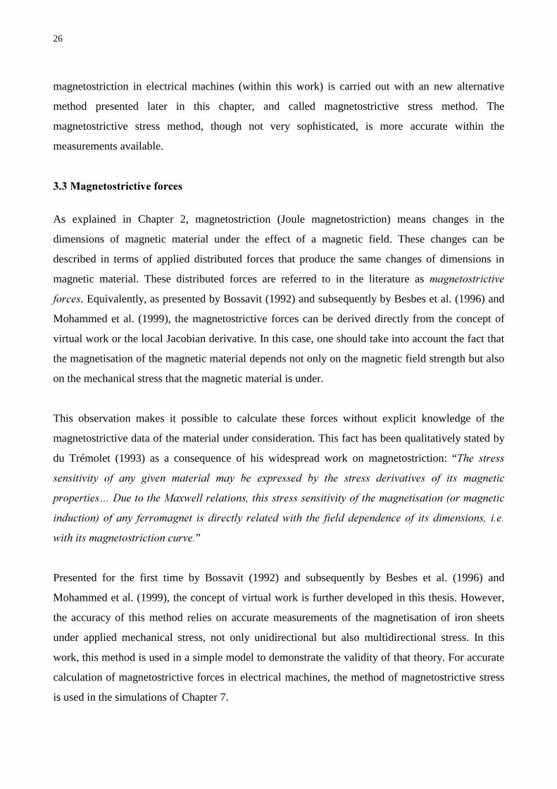
magnetostriction in electrical machines (within this work) is carried out with an new alternative
method presented later in this chapter, and called magnetostrictive stress method. The
magnetostrictive stress method, though not very sophisticated, is more accurate within the
measurements available.
,(,%#
As explained in Chapter 2, magnetostriction (Joule magnetostriction) means changes in the
dimensions of magnetic material under the effect of a magnetic field. These changes can be
described in terms of applied distributed forces that produce the same changes of dimensions in
magnetic material. These distributed forces are referred to in the literature as
$ . Equivalently, as presented by Bossavit (1992) and subsequently by Besbes et al. (1996) and
Mohammed et al. (1999), the magnetostrictive forces can be derived directly from the concept of
virtual work or the local Jacobian derivative. In this case, one should take into account the fact that
the magnetisation of the magnetic material depends not only on the magnetic field strength but also
on the mechanical stress that the magnetic material is under.
This observation makes it possible to calculate these forces without explicit knowledge of the
magnetostrictive data of the material under consideration. This fact has been qualitatively stated by
du Trémolet (1993) as a consequence of his widespread work on magnetostriction: “8&
$ & $
9*& & $&-
2$ $ & & $$ ''
& '”
Presented for the first time by Bossavit (1992) and subsequently by Besbes et al. (1996) and
Mohammed et al. (1999), the concept of virtual work is further developed in this thesis. However,
the accuracy of this method relies on accurate measurements of the magnetisation of iron sheets
under applied mechanical stress, not only unidirectional but also multidirectional stress. In this
work, this method is used in a simple model to demonstrate the validity of that theory. For accurate
calculation of magnetostrictive forces in electrical machines, the method of magnetostrictive stress
is used in the simulations of Chapter 7.
27
,(.%##
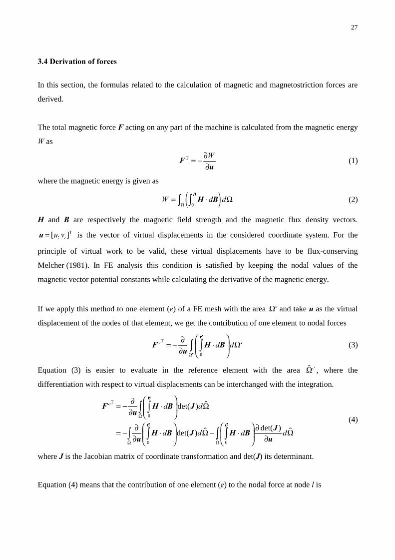
In this section, the formulas related to the calculation of magnetic and magnetostriction forces are
derived.
The total magnetic force acting on any part of the machine is calculated from the magnetic energy
as
T ∂= −∂
(1)
where the magnetic energy is given as
( )0
Ω= ⋅ Ω∫ ∫
%
(2)
and are respectively the magnetic field strength and the magnetic flux density vectors.
T[ ]O O
= is the vector of virtual displacements in the considered coordinate system. For the
principle of virtual work to be valid, these virtual displacements have to be flux-conserving
Melcher (1981). In FE analysis this condition is satisfied by keeping the nodal values of the
magnetic vector potential constants while calculating the derivative of the magnetic energy.
If we apply this method to one element () of a FE mesh with the area HΩ and take as the virtual
displacement of the nodes of that element, we get the contribution of one element to nodal forces
T
0H
H H Ω
∂= − ⋅ Ω ∂ ∫ ∫
%
(3)
Equation (3) is easier to evaluate in the reference element with the area ˆ HΩ , where the
differentiation with respect to virtual displacements can be interchanged with the integration.
T
ˆ 0
ˆ ˆ0 0
ˆdet( )
det( )ˆ ˆdet( )
H
Ω
Ω Ω
∂= − ⋅ Ω ∂ ∂ ∂= − ⋅ Ω − ⋅ Ω ∂ ∂
∫ ∫
∫ ∫ ∫ ∫
%
% %
(4)
where is the Jacobian matrix of coordinate transformation and det() its determinant.
Equation (4) means that the contribution of one element () to the nodal force at node is

28
H
H
[O
O
H
H
\O
O
%
%
∂= −∂
∂= −∂
(5)
Let us assume provisionally the constitutive equation of the material ( )2 ,ν= we may write
0 0
ν⋅ = ⋅∫ ∫% %
(6)
implying
0 0
1 2
22 2
20 0
3 4
2 2
0 0
( , ) ( , )
( , ) ( , )
ν
σν ν
σ
σ τν νσ τ
⊥
⊥
∂ ∂⋅ = ⋅ ∂ ∂
∂∂ ∂ ∂= ⋅ + ⋅ + ∂ ∂ ∂ ∂
∂ ∂ ∂ ∂⋅ + ⋅ ∂ ∂ ∂ ∂
∫ ∫
∫ ∫
∫ ∫
P
P
% %
% %
% %
(7)
The measurement of the reluctivity as function of the magnetic flux density and the unidirectional
mechanical stress and its development into two dimensional Fourier series in terms of the square of
the magnetic flux density and mechanical stress are described in Chapter 5.
Here, the measurement is provisionally supposed to be performed with the applied mechanical
stress and using its three components , andσ σ τ⊥P, respectively parallel and orthogonal to the
direction of and shear stress.
The first term of Eq. (7) can be calculated as follows
( )2
2 22
0
2
11 ( , )
2
1( , )
2
ν
ν
∂= ∂
=
∫%
(8)
This is half of the reluctivity of the element at the given values of flux density and mechanical
stress.
The second term of Eq. (7) is

29
22
2
0
1 ( , )2 ( )
2
σνσ
∂∂= ∂ ∂ ∫ P
P
%
(9)
The integration in Eq. (9) is done at constant stress since the measurement is performed at constant
externally applied stress and the effect of stress induced by magnetostriction is not considered. The
terms 3 and 4 of Eq. (7) are calculated in the same manner as term 2. The nodal forces are then
2 2
2 2
2T 2 2
ˆ 0 0
2 2
0 0
1 det( ) 1 1det( ) det( )
2 2 2
1 1 ˆdet( ) det( )2 2
H
σ νν νσ
σ ν τ νσ τ
Ω
⊥
⊥
∂∂ ∂ ∂= − + + + ∂ ∂ ∂ ∂∂ ∂ ∂ ∂ + Ω∂ ∂ ∂ ∂
∫ ∫ ∫
∫ ∫
P
P
% %
% %
(10)
For the evaluation of nodal forces, as well as for the evaluation of other terms that we will
encounter in the development of the coupling between magnetic and elastic fields, it is convenient
to present the reluctivity of the material as an m-dimensional cubic spline approximation with
respect to the square of the flux density 2 and the components of the mechanical stress. For
simplicity, and because the effect of the other stress components on the reluctivity is unknown, only
the component of stress parallel to the flux density is considered. On some interval
[ ]2 21 1, ,
N N K Kσ σ+ + × , the reluctivity is given by
2 2 2
0,30,3
( , ) ( ) ( )L M
NKLM N K
LM
ν σ σ σ==
= − −∑ (11)
The integration and differentiation of the reluctivity with respect to the variables 2 or σ is carried
out analytically using Eq. (11). In Eq. (10) there are derivatives of the flux density, the determinant
of the Jacobian matrix and stresses with respect to virtual displacements. These derivatives are
explicitly developed below.
The Jacobian matrix is given by
1, 1,
1, 1,
M M
M M
M Q M Q
M M
M M
M Q M Q
ξ ξ
η η
= =
= =
∂ ∂ ∂ ∂ = ∂ ∂ ∂ ∂
∑ ∑
∑ ∑ (12)
with the number of nodes in the element, the shape functions, ξ and η are the coordinates in the
reference frame.
The determinant of the Jacobian matrix is

30
11 22 12 21det( ) = − (13)
and the derivative of the determinant with respect to virtual displacements (which is the same as the
derivative with respect to nodal coordinates 0 0, = + = + ) is
22 12
11 21
det( )
det( )
O O
O
O O
O
ξ η
η ξ
∂ ∂ ∂ − ∂ ∂ ∂ =∂ ∂ ∂ − ∂ ∂ ∂
(14)
The flux density is calculated from the magnetic vector potential in a standard fashion
11 211,
22 121,
1
det( )
1
det( )
M M
M
M Q[
\ M M
M
M Q
η ξ
ξ η
=
=
∂ ∂ ∂ − ∂ ∂ ∂ = = ∂ ∂∂ − − ∂ ∂ ∂
∑
∑
(15)
using
2
2∂ ∂= ⋅∂ ∂
(16)
we still need to calculate ∂∂
, which is obtained from Eq. (15) and Eq. (14) as
1,
1 det( )
det( )
1 det( )
det( )
[ M MO O
M [
O M Q O
\
\
O O
ξ η ξ η=
∂ ∂ ∂ ∂ ∂ ∂− − ∂ ∂ ∂ ∂ ∂ ∂ = ∂ ∂− ∂ ∂
∑
(17)
and
1,
1 det( )
det( )
1 det( )
det( )
[[
OO
\ M MO O
M \
M QO O
ξ η ξ η=
∂ ∂ − ∂∂ = ∂ ∂ ∂ ∂ ∂ ∂− − ∂ ∂ ∂ ∂ ∂ ∂ ∑
(18)
The mechanical stress is given by
[ ] = (19)
where
[ ] 2
1 0
1 01
10 0
2
νν
νν
= − −
(20)

31
[ ] ( ) ( )
1 0
1 01 1 2
1 20 0
2
ν νν ν
ν νν
− = − + − −
(21)
1 1 2 2 3 3
∂ ∂ ∂ ∂ ∂ ∂ ∂ = ∂ ∂ ∂ ∂ ∂ ∂ ∂
σ σ σ σ σ σ σ(22)
so that
[ ] O O
∂ ∂=
∂ ∂ (23)
on the other hand
0
0
∂ ∂
∂ = ∂ ∂ ∂
∂ ∂
(24)
L L
L
=∑ and L L
L
=∑ (25)
so that
L
L
L
L
L
L
L L
L L
L L
∂ ∂ ∂ ∂
∂ ∂ ∂= ∂ ∂ ∂ ∂ ∂ ∂ ∂+ ∂ ∂ ∂ ∂
∑
∑
∑ ∑
(26)
and
[ ]
LL
LO
LL
LO O
L L
L L
L LO O
∂ ∂ ∂ ∂
∂ ∂ ∂= ∂ ∂ ∂ ∂ ∂ ∂ ∂+ ∂ ∂ ∂ ∂
∑
∑
∑ ∑
(27)
or more specifically, with , and the indices of the node of the element under consideration
(circular indices 1, 2 ,3 ,1 …)

32
[ ]
( )
( )
( ) ( )
M N L
LO
N M L
LO O
N M L M N L
L LO O
∂ − ∂ ∂ ∂= − ∂ ∂
∂ ∂− + − ∂ ∂
∑
∑
∑ ∑
(28)
[ ]( )
P Q
QP
Q P P Q
− = − − + −
(29)
Similarly
[ ]Q P
Q P
O
P Q Q P
− ∂ = − ∂ − + −
(30)
If the -axis is coincident with the direction defined by the flux density vector , we obtain the
derivatives for the plane stress case as:
2( ); 0
1 P Q
O O
σ σν
∂ ∂= − =
∂ − ∂P P (31)
2( ); 0
1 Q P
O O
σ σ
ν⊥ ⊥∂ ∂= − =
∂ − ∂(32)
2 2( ); ( )
1 1Q P P Q
O O
τ τ
ν ν∂ ∂= − = −∂ − ∂ −
(33)
However, there are no data available for the effect of multidirectional mechanical stress on the
magnetisation of iron. Furthermore, the effect of shear stress on the magnetic properties has never
been studied. In some publications (Schneider 1982, Kashiwaya 1991, Sablik 1993, 1995), there has
been an attempt to approach the effect of multidirectional stress in the same way as an equivalent
unidirectional stress. These different approximations are not accurate enough and sometimes they
are contradictory. The use of the developed formula for magnetostriction force is illustrated in a
calculation example below (3.7.2).
The method of virtual work developed above, although it gives good results for magnetic forces,
requires accurate measurement of the magnetisation versus applied mechanical stress to enable the
calculation of magnetostrictive forces.

33
From the measurement of magnetisation the derivative of the reluctivity with respect to
unidirectional stress can, in principle, be specified by iterating calculations and measurements.
Here, for simplicity, the derivative is specified from one cycle of measurements. Moreover, the
effect of orthogonal and shear stresses on magnetisation is unknown and its measurement is
complicated. For these reasons, the calculation of magnetostrictive forces is better carried out using
measured magnetostrictive stress versus magnetic flux density and applied mechanical stress. This
method, called the magnetostrictive stress method, is explained here.
First consider an element of iron in a magnetic field . Due to magnetostriction of iron, this
element will shrink or stretch depending on the sign of its magnetostriction. This change in
dimensions is described by a magnetostrictive strain tensor PV
. Corresponding to this strain, a
magnetostrictive stress tensor PV
can be calculated using Hook’s law. The nodal magnetostrictive
forces are calculated as the set of nodal forces due to this stress.
The measurement carried out and reported in Chapter 5 gives only the component of
magnetostrictive stress or strain in a direction parallel to that of the magnetic field. The other
component of magnetostrictive stress or strain orthogonal to the direction of the magnetic field
can be calculated within two assumptions. First, there is no magnetostrictive shear stress or strain in
the reference defined by the direction parallel to and the one orthogonal to it. Second, there is no
volume magnetostriction, which is a good assumption in the range of flux density occurring in
electrical machines. The latter assumption means that the magnetostriction strain in the direction
orthogonal to that of the magnetic field is opposite and has half the amplitude compared to the strain
parallel to the direction of the magnetic field.
The measurement described in Chapter 5 gives magnetostrictive stress PV
σPin a direction parallel to
that of the magnetic field as a two-dimensional cubic spline versus the magnetic flux density and the
applied mechanical stress. If PV
σ ⊥ is the magnetostrictive stress in a direction orthogonal to the
magnetic field, we can write, using the first assumption,
0 0
PV PV
PV PV
σ εσ ε⊥ ⊥
=
P P
(34)
The second assumption can be written as

34
1
2PV PVε ε⊥ = −
P(35)
So that, in the case of plane stress, we get
2 1
2PV PV
νσ σν⊥−=− P
(36)
The magnetostrictive nodal forces are calculated for each element as follows. Let θ be the angle
defined by the direction of the magnetic field and the x-axis. The projections of each edge of the
element in the directions parallel and orthogonal to the magnetic field are respectively
( ) ( )cos sin[ \
θ θ= +P
(37)
( ) ( )sin cos[ \
θ θ⊥ = − + (38)
where [ and \ are respectively the projection of the considered edge of the element on the - and -
axis. The forces, per unit length, parallel and orthogonal to the direction of the magnetic field are
respectively
PV PV σ=
P P P(39)
PV PV% σ⊥ ⊥ ⊥= (40)
These forces are distributed equally between the two nodes of the given edge. The forces in the
original Cartesian coordinate system are obtained as the projection of PV
%P and
PV% ⊥ on the axis of
that system
( ) ( )cos sinPV[ PV PV
% % %θ θ ⊥= −P
(41)
( ) ( )sin cosPV\ PV PV
% % %θ θ ⊥= +P
(42)
These forces are added to the magnetic nodal forces to get the nodal magnetic and magnetostrictive
forces. They can also be used separately in calculations to emphasise the effect of magnetostriction
only.
In a cartesian coordiante system the Maxwell stress tensor can be given as
2 2
2 2
0
2 2
1
21 1
21
2
[ [ \ [ ]
\ [ \ \ ]
] [ ] \ ]
: : : : :
: : : : :
: : : : :
− = − −
(43)

35
The Maxwell stress tensor can be applied to calculate the magnetic force acting on any part of the
machine e.g. the stator or rotor core of rotating electrical machines. If a closed surface M
Γ is chosen
as a cylinder in the air gap, closed through the end region of the machine, and with another
cylindrical surface outside the machine, the total force acting on the part considered can be deduced
as
j
j
2
0 0
2 2
0 0
1 1d
2
1 1( ) d
2
Q
Q W Q W
:
: : : :
= −
= − +
∫
∫
(44)
where the volume integral . d9
∇∫ is reduced to the closed surface integral of Eq. (44); and
stand respectively for the outward unit-vector normal to the differential surface dΓ and the
tangential one.
Since the integral on other surfaces than the one in the air gap is null, the integration in Eq. (44)
reduces to an integration over the cylindrical surface inside the air gap. The quantity inside the
integral of Eq. (44) is separated into the normal component (stress) and the circumferential
component (shear), respectively
2 2
0
1
2U U: :ϕ= − (45)
and
0
1U
: :ϕ ϕ= (46)
where the indices and have been replaced by and ϕ since the integration surface is now
cylindrical.
From the point of view of vibrations and noise analysis, it is important to know the spatial
distribution and the time dependence of the radial stress. For this purpose, the radial stress is
developed into a two-dimensional Fourier series
0 0
cos( )cos( ) cos( )sin( )
sin( )cos( ) sin( )sin( )
U PQ PQ PQ
P Q
PQ PQ
σ λ φ ω φ ω
φ ω φ ω
∞ ∞
= =
= + +
+
∑∑ (47)

36
where and are respectively space- and time-harmonic numbers, is the number of pole-pairs ω
is the rotational speed of the magnetic field, and φ are respectively the time and the angular
position. The other constants are given by
2 2
2 20 0 0
cos( )cos( )d d2
S
PQ U
ωω σ φ ω φµ
π π
=π ∫ ∫ (48)
2 2
2 20 0 0
cos( )sin( )d d2
S
PQ U
ωω σ φ ω φµ
π π
=π ∫ ∫ (49)
2 2
2 20 0 0
sin( )cos( )d d2
S
PQ U
ωω σ φ ω φµ
π π
=π ∫ ∫ (50)
2 2
2 20 0 0
sin( )sin( )d d2
S
PQ U
ωω σ φ ω φµ
π π
=π ∫ ∫ (51)
1for 0
41
21 for 0, 0
PQ
= == = > > =
> >
(52)
Equation (47) can be written as a sum of waves circulating forward (+) and backward (-) with
respect to the rotational direction of the rotor.
Hence, the radial stress can be written as
12 2 2
0 0
12 2 2
1 ( ) ( ) cos(- )
2
1( ) ( ) cos( )
2
U PQ PQ PQ PQ PQ
P Q
PQ PQ PQ PQ PQ
σ λ φ ω γ
λ φ ω γ
∞ ∞
+= =
−
= + + − + + +
− + + + +
∑∑(53)
In Eq. (53), the integer defines the mode or the spatial frequency of the radial stress components,
while defines the time frequency of these components. In the time stepping method, the
coefficients PQ, PQ, PQ and PQ are integrated at each step, and time-integrated from step to step so
that no post-processing is needed.

37
The nodal force method as described above and without magnetostriction has been used with a
simple benchmark model (Takahashi 1994). The model consists of a centre pole between yokes with
a small gap. The geometry of the device as presented by Takahashi et al. (1994) is shown in Fig. 6.
The geometry of the 2-D model and the FE mesh is shown in Fig. 7a. The calculated nodal forces
for that mesh are shown in Fig. 7b. The simulation is performed with a conventional magneto-static
FE program in Cartesian coordinates. The effect of saturation is taken into account in the form of a
nonlinear BH-magnetisation curve for the yoke and the pole.
The magnetisation curve used here is not the same as the one used in the reported benchmark of
Takahashi (1994). This missing information as well as the 2-D approach suggested that the
comparison of the forces should be made with known methods (Maxwell stress tensor and Lorentz
force) and not with measured results.
The mesh of Fig. 7a was adaptively refined. The total force acting on the iron pole and that on the
current carrying conductor are calculated. The nodal force method and either the Maxwell stress
tensor for the iron pole or the Lorentz formula for the conductor are used. The integration path for
the Maxwell stress tensor is kept the same regardless of the changed FE meshes. Fig. 8 shows the !-
components of the total force (calculated with the nodal forces method.) vs. the excitation current in
ampere-turns (AT)
%';)< $&& .-8.&&(//62'

38
Fig. 9 shows the !-components of the total forces vs. the number of nodes in the FE mesh at 1000
AT. The calculated forces agree with the results of the measured benchmark (Takahashi 1994) for
excitation currents of 5000 AT. At lower currents, the forces are much smaller. This can be caused
by the differences between the material magnetisation curves (not reported by Takahashi (1994))
and also by the 2-D approach. Moreover, the magnetisation curves used for the calculation of the
magnetic forces are linearised at low values of the magnetic field strength. This last procedure,
explained later in Chapter 6, makes the magnetic forces smaller at low values of the magnetic field
strength.
a) b)%'1)%&-2$ -2'
1
10
100
1000
10000
1000 2000 3000 4000 5000Exitation current (AT)
Fz (
N/m
)
Force on pole
Force on windings
%'0)% ' '

39
100
120
140
160
180
200
220
100 1000 10000 100000Node number
Fz (
N/m
)
Nodal forces
Maxwell stress
4
6
8
10
12
14
100 1000 10000 100000Node number
Fz
(N/m
) Nodal forcesLorentz force
a) b)%'/)% & -2&-2'
The results of this section are shown for the purpose of confirming the best accuracy of the method
of virtual work as compared to the Maxwell stress tensor for the calculation of total magnetic
forces. Although the two methods give the same result at high FE mesh density, the method of
virtual work (nodal forces) gives better results already at low FE mesh density. This result is in
accordance with the method used for the magnetic field calculation, which is based on the
minimisation of the energy. It is clear that the calculation of the forces from the energy is more
accurate than their calculation from field quantities which are calculated as derivatives of the
magnetic vector potential and include inaccuracies.
The calculation of magnetostrictive forces is carried out for a simple geometry with two different
methods to show the validity and accuracy of these methods.
The first method is the magnetostrictive stress method presented above where the magnetostrictive
forces are calculated directly from the measured magnetostrictive stress. The second method is the
energy derivative method presented above, which takes into account the dependency of
magnetisation on stress. The geometry is an iron core of width [= 0.2 m, thickness\ = 0.02 m
and infinitely long. The cross-section of the iron core is descretised into a 2-D FE mesh as shown in
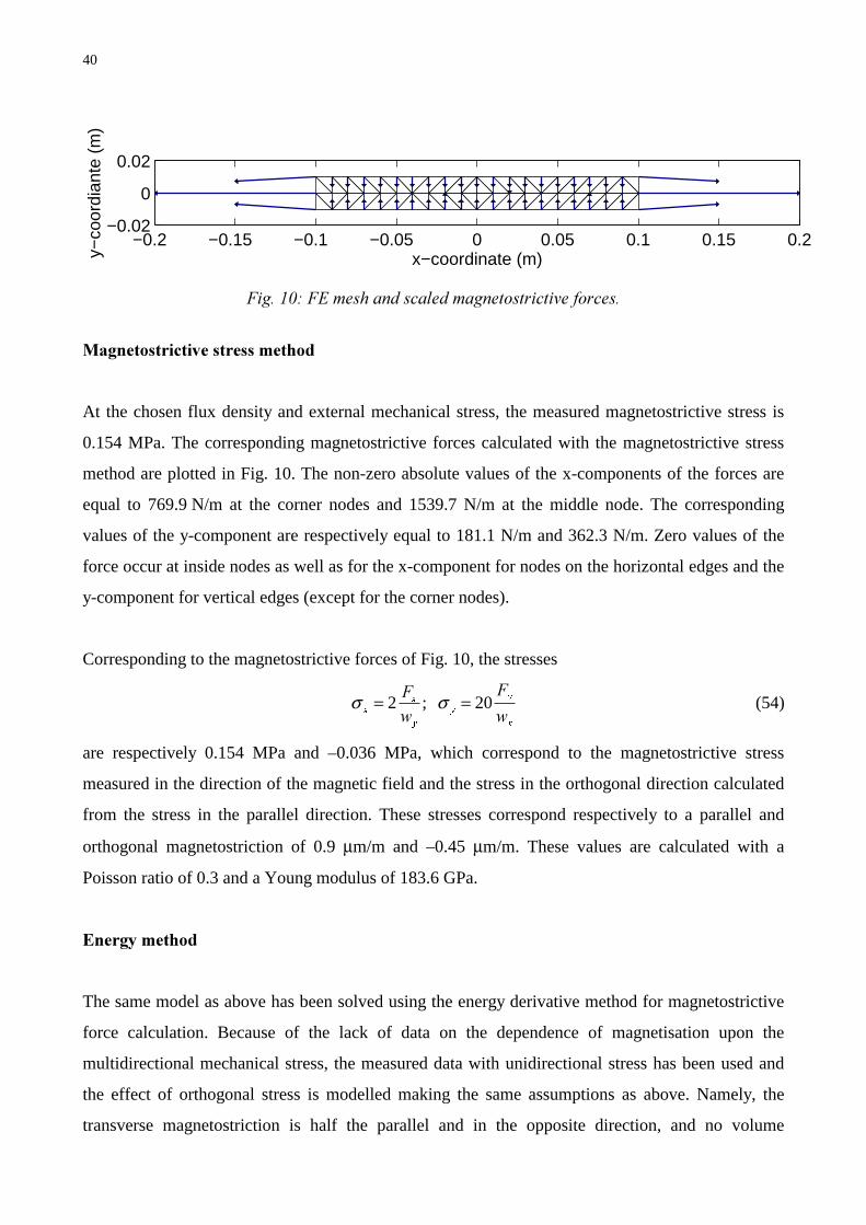
Fig. 10. The flux density is set to be constant and have a uniform value of 1 T in x-direction of the
Cartesian coordinate frame. The external mechanical stress is set to zero.
40
−0.2 −0.15 −0.1 −0.05 0 0.05 0.1 0.15 0.2−0.02
0
0.02
x−coordinate (m)y−co
ordi
ante
(m
)
%'(=)%& $ '
At the chosen flux density and external mechanical stress, the measured magnetostrictive stress is
0.154 MPa. The corresponding magnetostrictive forces calculated with the magnetostrictive stress
method are plotted in Fig. 10. The non-zero absolute values of the x-components of the forces are
equal to 769.9 N/m at the corner nodes and 1539.7 N/m at the middle node. The corresponding
values of the y-component are respectively equal to 181.1 N/m and 362.3 N/m. Zero values of the
force occur at inside nodes as well as for the x-component for nodes on the horizontal edges and the
y-component for vertical edges (except for the corner nodes).
Corresponding to the magnetostrictive forces of Fig. 10, the stresses
2 ; 20 \[
[ \
\ [
%%
σ σ= = (54)
are respectively 0.154 MPa and –0.036 MPa, which correspond to the magnetostrictive stress
measured in the direction of the magnetic field and the stress in the orthogonal direction calculated
from the stress in the parallel direction. These stresses correspond respectively to a parallel and
orthogonal magnetostriction of 0.9 µm/m and –0.45 µm/m. These values are calculated with a
Poisson ratio of 0.3 and a Young modulus of 183.6 GPa.
!
The same model as above has been solved using the energy derivative method for magnetostrictive
force calculation. Because of the lack of data on the dependence of magnetisation upon the
multidirectional mechanical stress, the measured data with unidirectional stress has been used and
the effect of orthogonal stress is modelled making the same assumptions as above. Namely, the
transverse magnetostriction is half the parallel and in the opposite direction, and no volume

41
magnetostriction occurs. The first assumption is taken into account only for the calculation of the
forces in the orthogonal direction; it is not the real effect of multidirectional stress on the
magnetisation.
The calculated forces are of the same form as in the magnetostrictive stress method; they can be
seen from Fig. 10. However, the corresponding values of the forces are the non-zero absolute values
of the -components equal to 3.32e+5 N/m at the corner nodes and 6.64e+5 N/m at the middle node.
The -components are respectively equal to 0.78e+5 N/m and 1.56e+5 N/m. Zero values of the force
occur at inside nodes as well as for the -component for nodes on the horizontal edges and the -
component for vertical edges (except for the corner nodes).
While the shape of the forces, their distribution and ratio are the same as in the magnetostrictive
stress method, their absolute values are more than 400 times larger than those calculated with this
method. These last ones agree well with the measurements. It is obvious that this difference is due
to the lack of information on the effect of multidirectional stress on the magnetisation. Indeed, in the
calculation of these forces, the effect of orthogonal stress on the magnetisation acts in the opposite
way to the stress in the parallel direction. This would result in a decrease of the forces as a result of
a decrease in the derivative of reluctivity, as can be seen from Eq. (10). Another cause of the
difference is the inaccuracy in the measurement of magnetisation. In this last measurement, only the
averaged single valued curves are taken. This is a good approximation for the magnetic field
computation, but it does not approximate well for the magnetostrictive force calculation.
The effect of mechanical stress on the magnetostrictive forces is shown using the example model
above. The force in the x-direction of the node in the middle of the right edge has been calculated at
various applied mechanical stresses. Fig. 11 shows the result of these calculations with both the
magnetostrictive stress method and the energy method; the flux density was 1 T.
The magnetostrictive forces show the same trend with respect to mechanical stress as reported by
Ruuskanen (1987). However, the forces calculated with the energy derivative method do not show
the saturation effect due to the mechanical stress. The forces calculated with the magnetostrictive
stress method show some fluctuations. This is not a real phenomenon; it is due only to the
representation of magnetostrictive stress with two-dimensional cubic splines and to measurement
inaccuracy.

42
−5 −4 −3 −2 −1 0 1 2 3 4 5−4
−2
0
2
4
6
8
10x 10
5
Mechanical stress (MPa)
For
ce (
N)
−5 −4 −3 −2 −1 0 1 2 3 4 5
−4000
−2000
0
2000
4000
6000
8000
10000
12000
Mechanical stress (MPa)
For
ce (
N)
-2 &-2 &%'(()*$& $ & '
0 0.2 0.4 0.6 0.8 1 1.2 1.4 1.6 1.80
2
4
6
8
10
12
14x 10
5
Flux density (T)
For
ce (
N)
0 0.2 0.4 0.6 0.8 1 1.2 1.4 1.6 1.8
−1000
0
1000
2000
3000
4000
5000
6000
7000
8000
9000
Flux density (T)
For
ce (
N)
-2 &-2 &%'(+)*$ $ &$ '
The change in magnetostrictive forces as a function of the flux density has also been checked by
setting the mechanical stress to 0 Pa and varying the flux density from 0 to 1.8 T. These results are
reported in Fig. 12. Here the trend is also almost the same for the two methods, but the absolute
values are different. Moreover, the decreases of magnetostriction at high flux densities are not seen
in the energy derivative method, neither is its correct behaviour seen at very low values of the
magnetic flux density.
Here, the method mentioned above that consists of developing the normal component of the
Maxwell stress tensor into a two-dimensional Fourier series is applied to a synchronous generator.
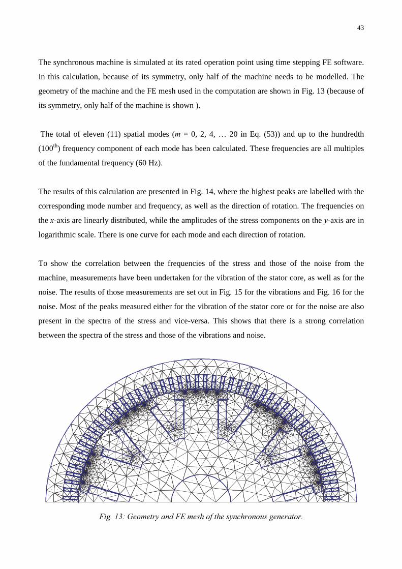
43
The synchronous machine is simulated at its rated operation point using time stepping FE software.
In this calculation, because of its symmetry, only half of the machine needs to be modelled. The
geometry of the machine and the FE mesh used in the computation are shown in Fig. 13 (because of
its symmetry, only half of the machine is shown ).
The total of eleven (11) spatial modes (= 0, 2, 4, … 20 in Eq. (53)) and up to the hundredth
(100th) frequency component of each mode has been calculated. These frequencies are all multiples
of the fundamental frequency (60 Hz).
The results of this calculation are presented in Fig. 14, where the highest peaks are labelled with the
corresponding mode number and frequency, as well as the direction of rotation. The frequencies on
the -axis are linearly distributed, while the amplitudes of the stress components on the -axis are in
logarithmic scale. There is one curve for each mode and each direction of rotation.
To show the correlation between the frequencies of the stress and those of the noise from the
machine, measurements have been undertaken for the vibration of the stator core, as well as for the
noise. The results of those measurements are set out in Fig. 15 for the vibrations and Fig. 16 for the
noise. Most of the peaks measured either for the vibration of the stator core or for the noise are also
present in the spectra of the stress and vice-versa. This shows that there is a strong correlation
between the spectra of the stress and those of the vibrations and noise.
%'(3)< %&$&& '
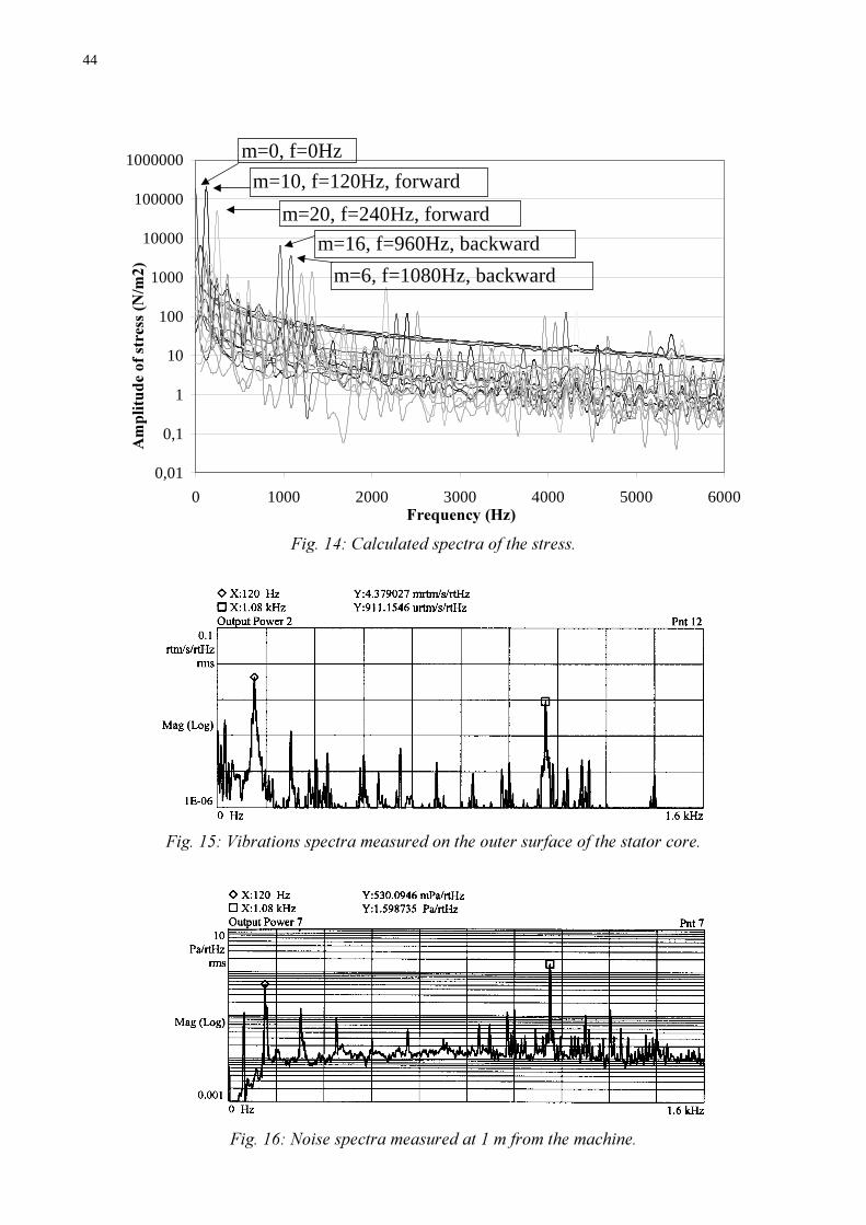
44
0,01
0,1
1
10
100
1000
10000
100000
1000000
0 1000 2000 3000 4000 5000 6000"#!$%&'
(
$
) '
m=10, f=120Hz, forward
m=20, f=240Hz, forward
m=16, f=960Hz, backward
m=6, f=1080Hz, backward
m=0, f=0Hz
%'(6)> $& '
%'(7) & $$& '
%'(;) ($ &&'
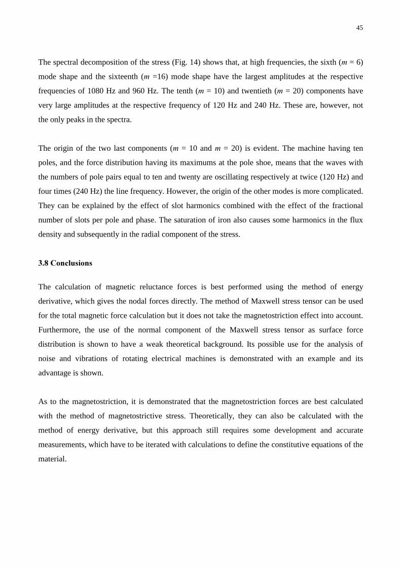
45
The spectral decomposition of the stress (Fig. 14) shows that, at high frequencies, the sixth ( = 6)
mode shape and the sixteenth ( =16) mode shape have the largest amplitudes at the respective
frequencies of 1080 Hz and 960 Hz. The tenth ( = 10) and twentieth ( = 20) components have
very large amplitudes at the respective frequency of 120 Hz and 240 Hz. These are, however, not
the only peaks in the spectra.
The origin of the two last components ( = 10 and = 20) is evident. The machine having ten
poles, and the force distribution having its maximums at the pole shoe, means that the waves with
the numbers of pole pairs equal to ten and twenty are oscillating respectively at twice (120 Hz) and
four times (240 Hz) the line frequency. However, the origin of the other modes is more complicated.
They can be explained by the effect of slot harmonics combined with the effect of the fractional
number of slots per pole and phase. The saturation of iron also causes some harmonics in the flux
density and subsequently in the radial component of the stress.
*+
The calculation of magnetic reluctance forces is best performed using the method of energy
derivative, which gives the nodal forces directly. The method of Maxwell stress tensor can be used
for the total magnetic force calculation but it does not take the magnetostriction effect into account.
Furthermore, the use of the normal component of the Maxwell stress tensor as surface force
distribution is shown to have a weak theoretical background. Its possible use for the analysis of
noise and vibrations of rotating electrical machines is demonstrated with an example and its
advantage is shown.
As to the magnetostriction, it is demonstrated that the magnetostriction forces are best calculated
with the method of magnetostrictive stress. Theoretically, they can also be calculated with the
method of energy derivative, but this approach still requires some development and accurate
measurements, which have to be iterated with calculations to define the constitutive equations of the
material.

46
,
In this chapter, the main equations for the magnetic and elastic field problems are introduced. The
different kinds of coupling between these two problems are explained and the coupling method used
in this work is developed. The aim of this chapter is to develop and present the equations needed for
the implementation of magnetoelastic software for the simulation of rotating electrical machines.
,
In this study, the magnetic field is calculated using the finite element method in two dimensions,
together with the time stepping scheme. The finite element method used here is based on the Φ−
formulation of the magnetic field, while the Crank-Nicholson method is used for time integration.
The electrical machines are treated as quasi-static magnetic systems (Arkkio 1987). In this case, the
Maxwell field equations reduce to
∂∇× = −∂
(55)
∇× = (56)
and the constitutive equations to
= (57)
= (58)
Using the vector potential and the reduced scalar potentialΦ defined by
= ∇× (59)
and
∂= − −∇∂
(60)
we get the equations for the vector and scalar potentials
(
σ σ∂∇× ∇× + + ∇ =∂
(61)
and
( ) ( ) 0
σ σ∂∇⋅ +∇ ⋅ ∇ =∂
(62)
For the sake of solution uniqueness, the "Coulomb gauge" is commonly used, i.e.
0∇⋅ = (63)
In the 2 dimensional case, the Coulomb gauge is satisfied implicitly.

47
The electrical machine is connected to the network and is usually voltage driven. In the two-
dimensional formulation, the voltage equation of conductors (with area )
S
d
σ ∂= + ⋅∂∫
(64)
has to be solved simultaneously with the field equations (61) and (62) (Arkkio 1987). The source of
the field being a known potential difference, the equation for the vector potential is
z(
∂∇× ∇× + =∂
(65)
where the potential difference between the ends of the conductors and the conductivityσ are
constant at every point on the cross section area of the conductor. is the length of the conductor. A
complete derivation of the above equations is given in Arkkio (1987).
The cross-section of the electrical machine is subdivided into triangular elements. The magnetic
vector potential is then approximated within each element in a standard fashion, and the potential
distribution in the various elements is constrained to be continuous across inter-element boundaries.
The system is discretised, and the set of equations obtained is solved using a computer program.
The nonlinearity of the iron requires an iterative solution process, in order to find the correct
solution of the vector potential, which also satisfies the material equations. This is achieved with the
Newton-Raphson iteration method (Zienkiewicz 1977).
In electrical machines, there is a rotor movement. Hence, the equations of movement, as well as the
changes in the geometry of the cross-section of the machine, have to be taken into account. The
equations of movement are solved with the FEM system of equation, while the change in the
geometry is brought about with the time-stepping method (Arkkio 1987).
In the time-stepping method, the time interval is also discretised into time steps of equal length. The
FE mesh of the region, between the static and moving parts of the machine, is regenerated after each
step. The system is solved at each step, taking into account the induced voltages due to the rotor’s
movement. A full description of the finite element method for electrical machines, as well as that of
the time stepping method, is given by Arkkio (1987).
In matrix form, the magnetic problem at each time step reduces to the following equations
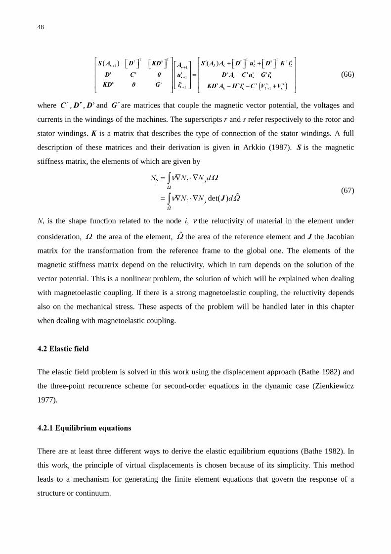
48
( )
( )
T T T Tr s r r s T s1 1
r r r r r r r r1
s s s s s s s s s1 1
( )N N N N N
N
N N N N
N N N N N
+ +
+
+ +
+ + = − − − − +
(66)
where U , U , V and V are matrices that couple the magnetic vector potential, the voltages and
currents in the windings of the machines. The superscripts and refer respectively to the rotor and
stator windings. is a matrix that describes the type of connection of the stator windings. A full
description of these matrices and their derivation is given in Arkkio (1987). is the magnetic
stiffness matrix, the elements of which are given by
ˆ
ˆdet( )
LM L M
L M
Ω
Ω
ν Ω
ν Ω
= ∇ ⋅∇
= ∇ ⋅∇
∫
∫ (67)
L is the shape function related to the node , ν the reluctivity of material in the element under
consideration, Ω the area of the element, Ω the area of the reference element and the Jacobian
matrix for the transformation from the reference frame to the global one. The elements of the
magnetic stiffness matrix depend on the reluctivity, which in turn depends on the solution of the
vector potential. This is a nonlinear problem, the solution of which will be explained when dealing
with magnetoelastic coupling. If there is a strong magnetoelastic coupling, the reluctivity depends
also on the mechanical stress. These aspects of the problem will be handled later in this chapter
when dealing with magnetoelastic coupling.
,
The elastic field problem is solved in this work using the displacement approach (Bathe 1982) and
the three-point recurrence scheme for second-order equations in the dynamic case (Zienkiewicz
1977).
, #-#
There are at least three different ways to derive the elastic equilibrium equations (Bathe 1982). In
this work, the principle of virtual displacements is chosen because of its simplicity. This method
leads to a mechanism for generating the finite element equations that govern the response of a
structure or continuum.

49
The domain under consideration is the stator core of the electrical machine. This domain can be
under the effect of surface tractions V , body forces % or concentrated forces L . These forces
include all externally applied forces and reactions and have in general three components
corresponding to the three coordinate axes
s B
s s B B
s B
; ;
L
[ [ [
L L
\ \ \
L
] ] ]
$ $ %
$ $ %
$ $ %
= = =
(68)
The displacements of the domain from the unloaded configuration are denoted by , where
[ ]T = (69)
The strains corresponding to these displacements are
T[[ \\ ]] [\ \] ][
ε ε ε γ γ γ = (70)
and the stresses corresponding to are
T[[ \\ ]] [\ \] ][
σ σ σ τ τ τ = (71)
The principle of virtual displacements states that the equilibrium of the domain requires that, for any
compatible, small virtual displacements (which satisfy the essential boundary conditions imposed
on the domain), the total internal virtual work is equal to the total external work:
T T B T S TS L L
L9 9 6
= + +∑∫ ∫ ∫ (72)
The internal virtual work is given on the left side of (72) and the external virtual work of the forces
is on the right side. The bar on the top of variables means they are virtual.
After FE discretisation, the displacements measured in a local coordinate system , , within each
element are approximated by
( ) ( ) ˆ( , , ) ( , , )P P = (73)
where ( )P is the displacement interpolation matrix, also called matrix of shape functions, and is
the vector of the three global displacement components at all nodal points
[ ]T1 1 1ˆ ...
Q = (74)
Although includes the displacements of all the nodal points, only the displacements at the nodes
of a given element affect the displacement and strain distributions in that element.
The strains in element are
( ) ( ) ˆ( , , ) ( , , )P P = (75)

50
where ( )P is the strain-displacement matrix, the rows of which are obtained from the rows of
( )P by appropriate differentiation and combinations.
The stresses are evaluated from the element strains and initial stresses ( )I P , if any, using
( ) ( ) ( ) ( )IP P P P= + (76)
where ( )P is the elasticity matrix of element .
Equation (72) is written as a sum of integrations over the volume and areas of all finite elements.
( ) ( ) ( )
T ( ) ( ) T B( ) ( ) T S( ) ( ) T( ) ( )S( )
P P P
P P P P P P LLP PP
9 9 6P P P L
= + +∑ ∑ ∑ ∑∫ ∫ ∫ (77)
Using the approximation in Eq. (73) and the relation of Eq. (76), Eq. (77) can be written in the
compact format
= (78)
where now contains the nodal displacements,
( )
( )
T ( ) ( )( ) ( )
P
P
P PP P
9P
= ∑ ∫
.
(79)
and
B C I S= + + + (80)
C = (81)
( )
( )I
T ( ) ( )( ) II
P
P
P PP
9P
= ∑ ∫
5
(82)
( )
S( )
T S( ) ( )( )S ( )
P
P
P PP P
6
6P
= ∑ ∫
5
(83)
The matrix ( )S P that appears in Eq.(83) is obtained from ( )P by substituting the element surface
coordinates.
Since this work deals with time-dependent fields, the effects of inertia and damping have to be
taken into account. This is done using d’Alembert’s principle, which includes the inertia forces as
part of the body forces. The damping forces are also included as velocity-dependent terms in the
body forces. So that

51
( )
T B( ) ( ) ( ) ( )( ) ( ) ( )
P
P P P PP P P
%
9P
ρ κ = − − ∑ ∫ (84)
Introducing Eq. (84) into Eq. (78) and rearranging gives the final second-order matrix-equation of
the elastic system
+ + = (85)
where
∂=∂
and
2
2∂=∂
are the first- and second-order derivatives of the nodal displacements
with respect to time and
( )
( )
T( ) ( )( ) ( )
P
P
P PP P
9P
ρ= ∑ ∫
0
(86)
( )
( )
T( ) ( )( ) ( )
P
P
P PP P
9P
κ= ∑ ∫
&
(87)
where ( )Pρ and ( )Pκ are respectively the mass density and damping property parameter of element
. The matrices , , and are respectively the mass, damping and stiffness matrices of the
system. These matrices are assembled in a standard fashion from element matrices ( )P , ( )P and
( )P . The knowledge of the parameter ( )Pκ is in general lacking. The damping matrix is then
evaluated using the so-called Rayleigh damping
α β= + (88)
with α and β appropriately chosen. These parameters can be calculated from two values of modal
damping at given frequencies. Reciprocally, the modal damping at any given frequency can be
estimated from the values of α and β . The choice of these parameters is explained in Chapter 7.
, . !
In the analysis of the elastic field of structures or continua, there are two kinds of boundary
conditions. The essential boundary conditions, also called or
and the natural boundary conditions, also called $ . The first
ones are the prescribed displacements or rotations, while the second ones are the applied external
forces. The latter are taken into account while evaluating the externally applied nodal-point force
vector. The displacement boundary conditions are handled in standard fashion (Bathe 1982).
Equation (85) is rewritten as
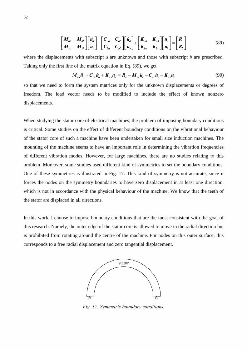
52
DD DE D DD DE D DD DE D D
ED EE E ED EE E ED EE E E
+ + =
(89)
where the displacements with subscript are unknown and those with subscript are prescribed.
Taking only the first line of the matrix equation in Eq. (89), we get
DD D DD D DD D D DE E DE E DE E+ + = − − − (90)
so that we need to form the system matrices only for the unknown displacements or degrees of
freedom. The load vector needs to be modified to include the effect of known nonzero
displacements.
When studying the stator core of electrical machines, the problem of imposing boundary conditions
is critical. Some studies on the effect of different boundary conditions on the vibrational behaviour
of the stator core of such a machine have been undertaken for small size induction machines. The
mounting of the machine seems to have an important role in determining the vibration frequencies
of different vibration modes. However, for large machines, there are no studies relating to this
problem. Moreover, some studies used different kind of symmetries to set the boundary conditions.
One of these symmetries is illustrated in Fig. 17. This kind of symmetry is not accurate, since it
forces the nodes on the symmetry boundaries to have zero displacement in at least one direction,
which is not in accordance with the physical behaviour of the machine. We know that the teeth of
the stator are displaced in all directions.
In this work, I choose to impose boundary conditions that are the most consistent with the goal of
this research. Namely, the outer edge of the stator core is allowed to move in the radial direction but
is prohibited from rotating around the centre of the machine. For nodes on this outer surface, this
corresponds to a free radial displacement and zero tangential displacement.
stator
%'(1) '

53
Since the degrees of freedom, on which the boundary conditions are imposed (i.e. radial and
tangential displacements), are not aligned with the global or local Cartesian coordinate system, we
need to express them in terms of the corresponding degrees of freedom of the defined assemblage
(i.e. displacements in the Cartesian coordinate system). Thus, we write
= (91)
with the vector of nodal displacements in the required direction. is an identity matrix that has
been altered by the direction cosines of the components in measured on the original displacement
direction. Equation (85) becomes
+ + = (92)
with
T T T T; ; ;= = = = (93)
In the two-dimensional approximation, two different approaches can be adopted. They are the plane
stress and plane strain.
The plane stress means that the only non-zero components of stress are in- plane. The other
components are zero. For the plane strain, the in-plane components of strain are non-zero and the
others are zero. Subsequently, the off-plane components of strain and stress respectively in plane
stress and plane strain are different from zero. However, their contributions to the internal work
vanish, since their counterparts, components of stress and strain, respectively, are zero.
The implementation of the plane stress or plane strain is the same; the only difference is in the
expression for the elasticity matrix[ ] . In this work, the plane stress approach was adopted, but the
computation routines are such that calculations with the plane strain approach are also possible. The
choice of one or other is more or less subjective. The main criterion behind this choice is the fact
that, in rotating electrical machines, both ends of the machine are allowed to move freely. This
situation corresponds better to the plane stress approach.
,
From the previous section, we obtained a second-order time-differential equation for the elastic field
problem. The solution of such an equation can be achieved using one of the recurrence schemes
summarised by Zienkiewicz (1977).
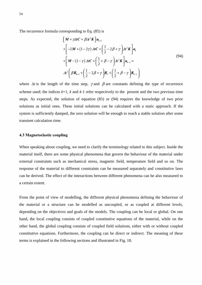
54
The recurrence formula corresponding to Eq. (85) is
( )
( )
21
2
21
21 1
12 1 2 2
2
11
2
1 12
2 2
N
N
N
N N N
γ∆ β∆
γ ∆ β γ ∆
γ ∆ β γ ∆
∆ β β γ β γ
+
−
+ −
+ + + − + − + − + + − − + + − = + − + + + −
(94)
where ∆ is the length of the time step, γ and β are constants defining the type of recurrence
scheme used; the indices .+1, . and .-1 refer respectively to the present and the two previous time
steps. As expected, the solution of equation (85) or (94) requires the knowledge of two prior
solutions as initial ones. These initial solutions can be calculated with a static approach. If the
system is sufficiently damped, the zero solution will be enough to reach a stable solution after some
transient calculation time.
,
When speaking about coupling, we need to clarify the terminology related to this subject. Inside the
material itself, there are some physical phenomena that govern the behaviour of the material under
external constraints such as mechanical stress, magnetic field, temperature field and so on. The
response of the material to different constraints can be measured separately and constitutive laws
can be derived. The effect of the interactions between different phenomena can be also measured to
a certain extent.
From the point of view of modelling, the different physical phenomena defining the behaviour of
the material or a structure can be modelled as uncoupled, or as coupled at different levels,
depending on the objectives and goals of the models. The coupling can be local or global. On one
hand, the local coupling consists of coupled constitutive equations of the material, while on the
other hand, the global coupling consists of coupled field solutions, either with or without coupled
constitutive equations. Furthermore, the coupling can be direct or indirect. The meaning of these
terms is explained in the following sections and illustrated in Fig. 18.

55
,/
Indirect coupling means that the magnetic, mechanical, thermal and other properties of the material
are not directly related to each other, either because we do not know the exact relation between
these properties, or because the dependence of one on the other is so small that we can ignore it. If
we ignore the coupling between materials’ properties we can still have a coupling between different
fields. Indirect coupling can be either weak (unidirectional) or strong.
0 1
The weak coupling is one possibility allowed by indirect coupling. It means that the effect of the
solution of one field on the other is only unidirectional. At a material-properties level, it also means
that the effect of the solution of one field on the properties related to the other field is ignored.
In magnetoelastic coupling, the weak coupling corresponds to the effect of the magnetic field on the
elastic field through magnetic forces, without any effect on the properties of the material. The
magnetic forces are then used as a load in the elastic field analysis. In this case, there is no back
effect of the elastic field on the magnetic field or on the magnetic properties of the material. This
approach is commonly used in the conventional design of electrical machines and apparatus that use
conventional materials such as iron, steel and copper and are not subject to very strict requirements
as to acoustic noise and vibrations.
Neither the effect of magnetostriction, nor the effect of geometrical changes due to elastic
displacement, can be taken into account accurately in such an analysis. The magnetostriction of iron
is stress sensitive within the range of stress occurring in electrical machines; the new geometry
requires new magnetic analysis either with FE, or analytically if we suppose linear behaviour.
The weak coupling is usually implemented so that the magnetic field is first solved with a computer
program or one of its components. Then, from the solution of the magnetic field, the magnetic
forces are calculated using one of the force calculation methods presented in Chapter 3. The
magnetic forces are then fed to another computer program that performs the elastic or mechanical
analysis to solve the displacement field from which different mechanical quantities can be
calculated (see). In this approach, the magnetic analysis is concerned with the electrical design of
the machine.

56
linear magnetic field
forces
elastic field
linear magnetic field
forces
elastic field
coupledmagnetoelastic field
a: weak b: strong c: direct
%'(0)%& $$$ .$'
It is meant to calculate the voltage, current, torque, power and other operational quantities. The
mechanical analysis on the other hand is meant to determine whether the mechanical parts of the
machine can stand the magnetic forces. The analysis checks the validity of the mounting, the
vibrational behaviour and possibly the noise of the machine.
Weak coupling is also used in magneto-thermal analysis, where the calculated electrical and
magnetic losses are used as load in the thermal problem. Only the approximate effect of temperature
on the resistance of conductors is taken into account. Usually, the solution of the thermal analysis is
not used to calculate the exact resistance corresponding to the calculated temperature.
2
The indirect coupling can be implemented also as strong coupling. In this case, not only the effect of
the magnetic field on the elastic one is taken into account, but also the effect of the elastic field on
the magnetic one is accounted for. This kind of analysis is necessary if the mechanical stress in the
machine is so high that it changes the magnetic properties of the material. The elastic displacement
field can also change the geometry of the machine and affect the solution of the magnetic field. The
strong coupling requires an iterative procedure using either the same computer program or different
programs to solve the magnetic and elastic field.
In FE analysis, the indirect coupling, either weak or strong, is implemented by assembling different
system matrices for the magnetic and elastic field. Moreover, the elastic and magnetic properties of
the material are separated. The Poisson ratio and Young modulus do not depend on the magnetic
field, while the magnetic permeability is either not dependent on mechanical stress (weak coupling)
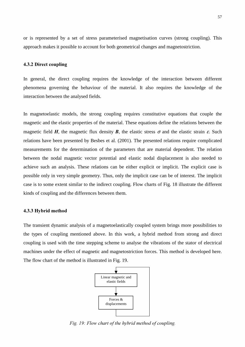
57
or is represented by a set of stress parameterised magnetisation curves (strong coupling). This
approach makes it possible to account for both geometrical changes and magnetostriction.
, 3
In general, the direct coupling requires the knowledge of the interaction between different
phenomena governing the behaviour of the material. It also requires the knowledge of the
interaction between the analysed fields.
In magnetoelastic models, the strong coupling requires constitutive equations that couple the
magnetic and the elastic properties of the material. These equations define the relations between the
magnetic field , the magnetic flux density , the elastic stress σ and the elastic strain ε. Such
relations have been presented by Besbes et al. (2001). The presented relations require complicated
measurements for the determination of the parameters that are material dependent. The relation
between the nodal magnetic vector potential and elastic nodal displacement is also needed to
achieve such an analysis. These relations can be either explicit or implicit. The explicit case is
possible only in very simple geometry. Thus, only the implicit case can be of interest. The implicit
case is to some extent similar to the indirect coupling. Flow charts of Fig. 18 illustrate the different
kinds of coupling and the differences between them.
,%!-
The transient dynamic analysis of a magnetoelastically coupled system brings more possibilities to
the types of coupling mentioned above. In this work, a hybrid method from strong and direct
coupling is used with the time stepping scheme to analyse the vibrations of the stator of electrical
machines under the effect of magnetic and magnetostriction forces. This method is developed here.
The flow chart of the method is illustrated in Fig. 19.
Linear magnetic andelastic fields
Forces &displacements
%'(/)%& $&& &$'
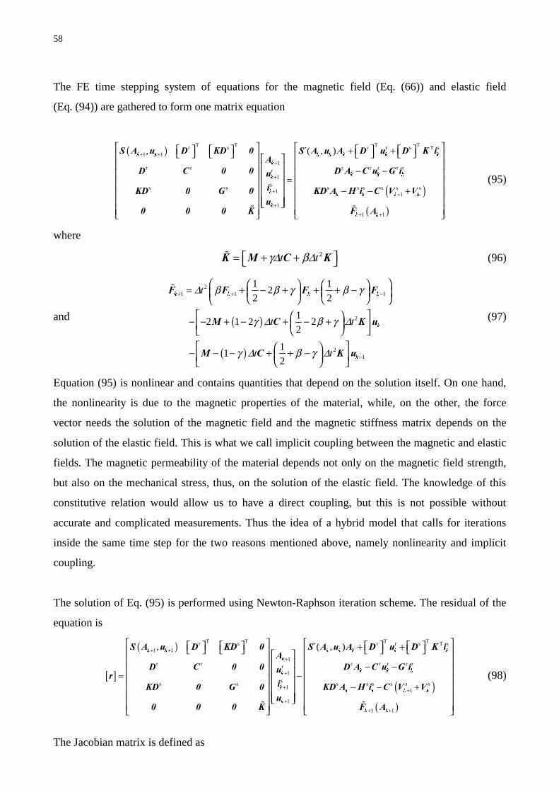
58
The FE time stepping system of equations for the magnetic field (Eq. (66)) and elastic field
(Eq. (94)) are gathered to form one matrix equation
( )
( )( )
T T T Tr s r r s T s1 1
1r r r r r r rr
1s
s s s s s s s s1
1
1
1 1
, ´( , )N N N N N N N
N
N N NN
NN N N N
N
N N
+ ++
+
+ +
+
+ +
+ + − − = − − +
(95)
where
2 γ∆ β∆ = + + (96)
and ( )
( )
21 1 1
2
21
1 12
2 2
12 1 2 2
2
11
2
N N N N
N
N
∆ β β γ β γ
γ ∆ β γ ∆
γ ∆ β γ ∆
+ + −
−
= + − + + + − − − + − + − + − − − + + −
(97)
Equation (95) is nonlinear and contains quantities that depend on the solution itself. On one hand,
the nonlinearity is due to the magnetic properties of the material, while, on the other, the force
vector needs the solution of the magnetic field and the magnetic stiffness matrix depends on the
solution of the elastic field. This is what we call implicit coupling between the magnetic and elastic
fields. The magnetic permeability of the material depends not only on the magnetic field strength,
but also on the mechanical stress, thus, on the solution of the elastic field. The knowledge of this
constitutive relation would allow us to have a direct coupling, but this is not possible without
accurate and complicated measurements. Thus the idea of a hybrid model that calls for iterations
inside the same time step for the two reasons mentioned above, namely nonlinearity and implicit
coupling.
The solution of Eq. (95) is performed using Newton-Raphson iteration scheme. The residual of the
equation is
[ ]
( )
( )( )
T T T Tr s r r s T s1 1
1r r r r r r rr
1s
s s s s s s s s1
1
1
1 1
, ´( , )N N N N N N N
N
N N NN
NN N N N
N
N N
+ ++
+
+ +
+
+ +
+ + − − = − − − +
(98)
The Jacobian matrix is defined as
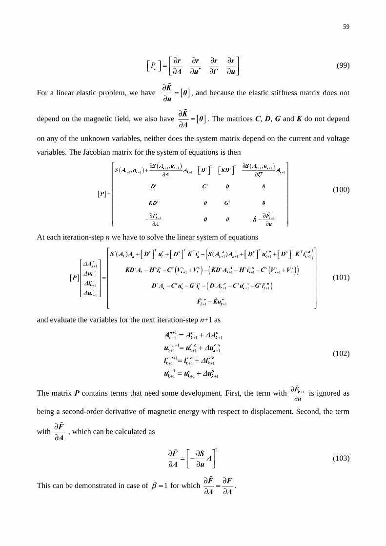
59
LM U V5
∂ ∂ ∂ ∂ = ∂ ∂ ∂ ∂
(99)
For a linear elastic problem, we have [ ]∂ =∂
, and because the elastic stiffness matrix does not
depend on the magnetic field, we also have [ ]∂ =∂
. The matrices , , and do not depend
on any of the unknown variables, neither does the system matrix depend on the current and voltage
variables. The Jacobian matrix for the system of equations is then
[ ]
( ) ( ) ( )T T1 1 1 1r s1 1 1 1
r r
s s
1 1
, ,, N N N N
N N N N
N N
+ + + ++ + + +
+ +
∂ ∂ + ∂ ∂
=
∂ ∂ − − ∂ ∂
% %
%
6 $ X 6 $ X6 $ X $ ' .' $
$ 8
' &
3
.' *
) ) .
$ X
(100)
At each iteration-step we have to solve the linear system of equations
[ ]
( )( ) ( )( )
T T T Tr r s T s r r s T s1 1 1 1
1 s s s s s s s s s s s s1 1 1 1
1
r r r r r r r11
1
´( ) ( )Q Q Q Q
N N N N N N N N
Q
NQ Q
U QN N N N N N N N
N
V Q
QN
N N N N N
Q
N
∆∆∆∆
+ + + +
+
+ + + ++
++
+
+ + − + + − − + − − − + = − − − −
( )r r r1 1
1 1
Q Q
N
Q Q
N N
+ +
+ +
−
−
(101)
and evaluate the variables for the next iteration-step +1 as
11 1 1
11 1 1
11 1 1
11 1 1
Q Q Q
N N N
U Q U Q U Q
N N N
V Q V Q V Q
N N N
Q Q Q
N N N
∆∆
∆∆
++ + +
++ + ++
+ + +++ + +
= +
= +
= +
= +
(102)
The matrix contains terms that need some development. First, the term with 1N+∂∂
is ignored as
being a second-order derivative of magnetic energy with respect to displacement. Second, the term
with ∂∂
, which can be calculated as
T∂ ∂ = − ∂ ∂
(103)
This can be demonstrated in case of 1β = for which ∂ ∂=∂ ∂
.

60
T
0
T
∂ ∂ ∂= −∂ ∂ ∂
∂ ∂= −∂ ∂
∂ = − ∂
∫$
(104)
In Eq. (104), the symmetry 7 = has been used as well as the alternative expression for magnetic
energy in terms of FE variables. The equality in Eq. (103) renders the system matrix symmetric. The
term with ∂∂
can be assembled from the same term calculated at element level
1 1 2 2 3 3
H H H H H H H
∂ ∂ ∂ ∂ ∂ ∂ ∂= ∂ ∂ ∂ ∂ ∂ ∂ ∂
(105)
the elements of which are given by
( )
ˆ
(1)
ˆ
(2)
ˆ
ˆdet( )
ˆdet( )
ˆdet( )
LM
L M
O O
L M
O
L M
O
Ω
Ω
Ω
ν Ω
ν Ω
ν Ω
∂ ∂ = ∇ ⋅∇ ∂ ∂
∂ = ∇ ⋅∇ + ∂
∂ ∇ ⋅∇ ∂
∫
∫
∫
(106)
with
( )2
ˆ
,ˆterm1 det( )
L M
O
Ω
νΩ
∂ = ∇ ⋅∇ ∂∫
(107)
and
( ) ( )ˆ ˆ
det( ) ˆ ˆterm2 det( )L M
L M
O O
Ω Ω
ν Ω ν Ω ∂ ∇ ⋅∇∂ = ∇ ⋅∇ + ∂ ∂∫ ∫
(108)
In Eq. (107), we have
( )2 2
2
,
O O O O O
ν σν ν ν σ ν τσ σ τ
⊥
⊥
∂ ∂∂ ∂ ∂ ∂ ∂ ∂ ∂= + + +∂ ∂ ∂ ∂ ∂ ∂ ∂ ∂ ∂
P
P
(109)
If we consider only the effect of unidirectional mechanical stress in the direction of the flux density
, we get

61
( )
2
2ˆ
det( )det( )
ˆdet( )
LM
L M
O O O O
L M
O
Ω
ν ν σ νσ
ν Ω
∂ ∂ ∂ ∂ ∂ ∂ = + + ∇ ⋅∇ + ∂ ∂ ∂ ∂ ∂ ∂ ∂ ∇ ⋅∇ ∂
∫
(110)
where the terms with 2
ν∂∂
, 2
O
∂∂
,νσ
∂∂
,Oσ∂
∂ and
det( )
O
∂∂
have been developed in the force
calculation and the terms with L M
∇ ⋅∇ and det( ) are calculated in a standard fashion.
We also have the following terms needed for the calculation of Eq. (110)
21 21 11
2
11 21 11
det( )
det( )
21
det( )2
L M OL M
O
MO L O O L
MO L O O L
η ξ ξ η η ξ
ξ η ξ η ξ η
∂ ∂∇ ⋅∇ ∂= − ∇ ⋅∇ +
∂ ∂ ∂ ∂ ∂ ∂ ∂− + + ∂ ∂ ∂ ∂ ∂ ∂ ∂ ∂ ∂ ∂ ∂ ∂ − + ∂ ∂ ∂ ∂ ∂ ∂
(111)
and
22 22 12
2
12 22 12
det( )
det( )
21
det( )2
L M OL M
O
MO L O O L
MO L O O L
η ξ ξ η η ξ
ξ η ξ η ξ η
∂ ∂∇ ⋅∇ ∂= − ∇ ⋅∇ +
∂ ∂ ∂ ∂ ∂ ∂ ∂− + + ∂ ∂ ∂ ∂ ∂ ∂ ∂ ∂ ∂ ∂ ∂ ∂ − + ∂ ∂ ∂ ∂ ∂ ∂
(112)
In the calculations of Chapter 7, the coupling terms between the magnetic and elastic problems in
the system matrix are small compared to the other terms. This results in an ill-conditioned matrix
that would require extra conditioning for the coupled problem. However, this procedure was not
needed, since the iteration process converged without these coupling terms, but with an extra
iteration at each step. On one hand, this makes the calculation time longer; on the other, it saves
time, since no conditioning is needed.
In systems with large displacements or a strong dependency of the force on the magnetic vector
potential (i.e. on the magnetic field distribution), the solution process would require either a
62
conditioning of the matrix or many more iterations. In that case, an estimation of the calculation
time for both processes is needed to make a choice that minimises the global calculation time. This
situation will be experienced when both the magnetoelastic coupling and the stress-dependency of
the magnetostrictive forces are taken into account in Chapter 7. Indeed, in that case, the iteration
process does not converge.
,,+
Different kinds of magnetoelastic coupling have been presented and discussed. A hybrid method of
magnetoelastic coupling has been introduced and the equations related to this method have been
derived from the magnetic and elastic field equations.
It is shown that the effect of mechanical stress on the magnetostriction of magnetic materials can be
taken into account only in a strong coupling approach either directly or indirectly. The introduced
hybrid method of coupling is able to account for both the geometrical changes and the
magnetostriction with its stress dependency.
The Hybrid method for magnetoelastic coupling is used in the coupled calculations of Chapter 7.
The stress-dependency of the magnetic properties (only the magnetostriction) is taken into account
in separate cases to show their effect on the vibrations.

63
The aim of this chapter is to introduce a device for measuring the magnetic properties of electrical
steel sheets, and to describe the set-up of the device. The measured properties are the magnetic flux
density versus the magnetic field strength, together with the externally applied mechanical stress,
and the magnetostrictive stress versus the magnetic flux density, together with the externally applied
mechanical stress. The measurements demonstrate the dependency of the measured quantities on the
applied mechanical stress. The results of these measurements are developed in a form adequate for
further use in the computations of Chapters 6 and 7.
The FE computation of magnetic fields in electrical machines requires knowledge of the magnetic
properties of materials used in the machine. Among these properties, the specific total loss and the
magnetisation data of magnetic materials are needed. The manufacturers of electrical steel sheets
usually provide these properties.
There are several standard methods for the measurement of magnetic properties of magnetic
materials. One of the most widely used methods is the 25 cm Epstein frame method (IEC 60404-2
1996). These methods give the magnetisation data as a function of magnetic field strength; the
specific total loss is given as a function of magnetic flux density.
However, the calculation of magnetic and magnetostriction forces as described in Chapter 3, as well
as the magnetoelastic coupling as described in Chapter 4, requires more complex material
properties. These are the magnetisation and the magnetostriction data, not only as a function of the
magnetic field strength or magnetic flux density, but also as a function of the externally applied
mechanical stress. This kind of data is not standard, neither is it provided by the manufacturers of
electrical steel sheets. In this work, the measurement of such data was conducted using a slightly
modified version of the 25 cm Epstein frame. The modifications mainly involve the dimensions of
the test specimen and the use of extra insulation between strips. These modifications are necessary
to allow for the application of externally applied mechanical stress. This particular modification was
applied and measured by a system of screws and load cells as shown in Fig. 20. A photo of the
Epstein frame is shown in Fig. 21.

64
1
2
3 4
5
5
5 5
!!!"#$!$!%
&!!!#$'!%
The screw system allowed for the application of both tensile (positive) and compressive (negative)
mechanical stresses. The use of plastic strips in between the iron strips prevented them bending
when compressive stress was applied.
The measurement set-up for the stress-dependent magnetisation data is shown in Fig. 22. The dc-
measurement method was used. The mechanical stress was varied from a value of –5.23 MPa to
5.23 MPa by steps of 0.436 MPa. At each step, the dc-measurement of the magnetisation was
carried out by changing the primary current from a minimum value to a maximum one and back to
the first value in very small steps, very slowly.

65
())
−2 −1.5 −1 −0.5 0 0.5 1 1.5 2
x 104
−2
−1.5
−1
−0.5
0
0.5
1
1.5
2
Magnetic field strength H (A/m)
Mag
netic
flux
den
sity
B (
T)
($!*!!$!!
The corresponding maximum and minimum values of the average magnetic field strength in iron
were calculated from the measured current as, respectively, –18 kA/m and 18 kA/m and those of the
magnetic flux density were calculated from the induced voltage as, respectively, –1.8 T and 1.8 T.
The measured hysteresis loop at no mechanical stress (σ = 0) is shown in Fig. 23. Single-valued
magnetisation curves were calculated from the hysteresis loops at each value of the applied
mechanical stress. The calculation procedure for single-valued magnetisation and magnetostriction
curves is explained later in this chapter. The positive parts of the single-valued curves (first
quadrant) were taken as magnetisation data for the electrical steel sheet. These magnetisation curves
are shown in Fig. 24 as functions of applied mechanical stress. Further, the parameterised
magnetisation curves have been developed into two-dimensional cubic spline form to make their
use easy within the FE computation and to enable the calculation of the magnetoelastic coupling
terms developed in Chapter 4.

66
0 100 200 300 400 5000
0.2
0.4
0.6
0.8
1
1.2
1.4
Magnetic field strength H (A/m)
Mag
netic
flux
den
sity
B (
T)
σ↑
(*!!$!!
−6−4
−20
24
6
0
1
2
30
1000
2000
3000
4000
5000
Applied mechanical stress (MPa)
square of the magnetic flux density (T2)
Rel
uctiv
ity (
Vs/
Am
)
−5
0
50
0.51
1.52
x 104
0
0.5
1
1.5
2
Magnetic field strength (A/m)
Applied mechanical stress (MPa)
Mag
netic
flux
den
sity
(T
)
%+!$'%"&!'!
A plot of the two-dimensional cubic spline approximation of the reluctivity is shown in Fig. 25a.
The corresponding plot of the magnetisation data is shown in Fig. 25b. The development of the
measured data into two-dimensional cubic spline was performed using standard and own routines in
a commercial software package (Matlab © university version 6.01).
The results of Fig. 25 were used in the calculation of magnetostrictive forces in the example of
Section 3.7.2 in conjunction with the method of energy derivative presented in Chapter 3.
The measurement of magnetostriction was conducted using the same set-up as for the measurement
of magnetisation. The only difference is the piezo-electric force transducer introduced between the

67
load cell and the specimen holder. The transducer was used for the measurement of the force due to
magnetostriction in the direction parallel to the magnetic field. The magnetic field density measured
by the integrator, as well as the magnetic field strength calculated from the current of the primary
winding and the magnetostrictive forces measured by the piezo-electric transducer, were collected
in the measurement computer as functions of time. The measurement frequency was 5 Hz.
The mechanical stress was varied as in the measurement of magnetisation from –5.23 MPa to 5.23
MPa by steps of 0.436 MPa. At each step, the magnetic field was varied from –18 kA/m to 18 kA/m
by varying the current of the primary winding of the Epstein frame. The corresponding maximum
and minimum values of the magnetic field density were –1.8 T and 1.8 T. Each step of measurement
produced a magnetostrictive hysteresis loop that consisted of magnetostrictive stress as a function of
magnetic field density. The procedure of calculating those loops from measured forces is explained
later in this chapter. One such hysteresis loop measured at a mechanical stress of 0.0 Pa is shown in
Fig. 26a. The corresponding magnetostriction loop is shown in Fig. 26b. The magnetostrictive
hysteresis loops were averaged to obtain single-valued magnetostrictive curves at different values of
the applied mechanical stress. Some of these curves are shown in Fig. 27a. The corresponding
magnetostriction is shown in Fig. 27b.
For a better use of the magnetostrictive data in computations, these data were presented in the so-
called two-dimensional cubic spline form as a function of the magnetic field density and the applied
mechanical stress. Such a representation is shown in Fig. 28. The data presented in Fig. 28 are used
in the simulations of Chapter 7, as well as in the example in 3.7.2, in conjunction with the method
of magnetostrictive stress.
−2 −1.5 −1 −0.5 0 0.5 1 1.5 2−2
0
2
4
6
8
10x 10
5
Magnetic flux density B (T)
Mag
neto
stric
tive
stre
ss (
Pa)
−2 −1.5 −1 −0.5 0 0.5 1 1.5 2
−2
0
2
4
6
8
10
12x 10
−7
Magnetic flux density B (T)
Mag
neto
stric
tion
(m/m
)
%'%,($! &

68
−2 −1.5 −1 −0.5 0 0.5 1 1.5 2−1
−0.5
0
0.5
1
1.5
2
2.5
3
3.5x 10
6
Flux density (T)
Mag
neto
stric
tive
stre
ss (
Pa)
3.9 MPa0.0 MPa−1.7 MPa−6.1 MPa
−2 −1.5 −1 −0.5 0 0.5 1 1.5 2
−2
−1
0
1
2
3
4
5x 10
−6
Flux density (T)
Mag
neto
stric
tion
(m/m
)
3.9 MPa0.0 MPa−1.7 MPa−6.1 MPa
%'%-(!!!
−5
0
5
0
1
2−1
0
1
2
3
4
x 106
Applied mechanical stress (MPa)Magnetic flux density (T)
Mag
neto
stric
tive
stre
ss (
Pa)
.&!#)!'!
+ 4
The measured hysteresis curves, both of magnetisation and magnetostriction, contain measurement
noise and need to be filtered. Furthermore, the data needed for computation have to be single-
valued. For these reasons, the measurement results have been handled as follows.
The data points are reordered to obtain smooth curves. The descending hysteresis branch is
resampled at the same abscisses as the ascending one and the average ordinates are taken as single
values (see Fig. 29). This procedure corresponds to the interpolation of the flux density of the
descending branch of the magnetisation curve at a given measured value of the magnetic field
strength on the ascending branch. The single value of the magnetic flux density corresponding to the
measured magnetic field strength on the ascending branch is the average value of the measured flux
density on the ascending branch and the interpolated one on the descending branch.

69
/0!!
The same procedure is applied to the magnetostrictive stress, where the abscisse is now the
magnetic flux density and the ordinate is the magnetostrictive stress. Fig. 29 illustrates the
averaging procedure.
,+
The presented device for measuring magnetostriction gives a force from which the magnetostriction
and the magnetostrictive stress need to be calculated. The procedure for calculating these quantities
is presented here.
One strip of the measurement device with its supports and holders, can be schematised as shown in
Fig. 30a. This part is mechanically equivalent to the system of springs shown in Fig. 30b. The force
measured by the piezo-electric force transducer is the force in the system of springs at equilibrium
after the magnetostriction takes place. Since the measurement is made at a frequency of 5 Hz, the
mass effect can be ignored. The spring constants of the iron strip, the force transducer, the load cell
and the support are respectively kiron=1.7E+8 N/m, kFT=1E+8 N/m, kLC=5E+8 N/m, and
ksupport=5E+6 N/m. The elongation of each spring at equilibrium can be calculated from the
measured force and the spring constants in a conventional way as
*1
∆ = . The elongation of the
iron due to the magnetostriction is then the sum of the elongations of each spring.
H2H1 H3
B1
B2
B3Bi
Ba
Measured points
Interpolated point
Averaged = single value point

70
%!!! '%2!
2!
To produce the same magnetostrictive elongationλ in the iron, a force PV LURQ
1 λ= − is needed. The
magnetostrictive stress is calculated as the stress due to this magnetostrictive force i.e. PV
PV
σ = ,
being the cross section of the iron strip.
+
A simple but sufficiently accurate measurement device is presented. The measurement set-up
enables measurements of both magnetisation and magnetostriction as functions of the externally
applied stress.
The measurement results show a strong dependency of the magnetostriction on the externally
applied mechanical stress, while the dependency of the magnetisation on the mechanical stress is
strong only at low values of the magnetic field strength and at the knee of the magnetisation curve.
The measured data have been developed into a format adequate for further use in FE computations
of electrical machines.
3 2 1
4
44
kiron kFT kLC ksupport
Before MS
After MS

71
5
The method developed in this work to calculate magnetic and magnetostrictive forces and
magnetoelastic coupling is first validated with a validation device. It is then applied to the analysis
of synchronous and induction machines. The results of measurements using the validation device,
and of computations made on it, are presented below.
The validation device was constructed to verify the calculation of magnetic and elastic fields and
magnetostriction forces. The goal was to design a motor-like device in which the reluctance or
Maxwell forces were minimal, causing it to vibrate under the effect of magnetostrictive forces only.
A comparison of the calculation results with those from measurements would confirm the validity
of the calculation method. The results of the measurements would verify the nature of the vibrations
of rotating electrical machines under the effect of magnetostriction.
2
The validation device consists of an induction machine in which the rotor has not been cut from the
stator. The device is, then, just like a induction machine, short in axial length and without an air
gap. The rotor part (if it can be called such) of the machine is different from a normal machine in
the sense that it has no windings. This device was designed, construct and measured within this
research work (the design and construction were done as a master’s thesis (Cester 2002) in the
Laboratory of Electromechanics at Helsinki University of Technology). Its geometrical and
electrical parameters are given in Appendix A. Fig. 31 shows a photo of this device.
!
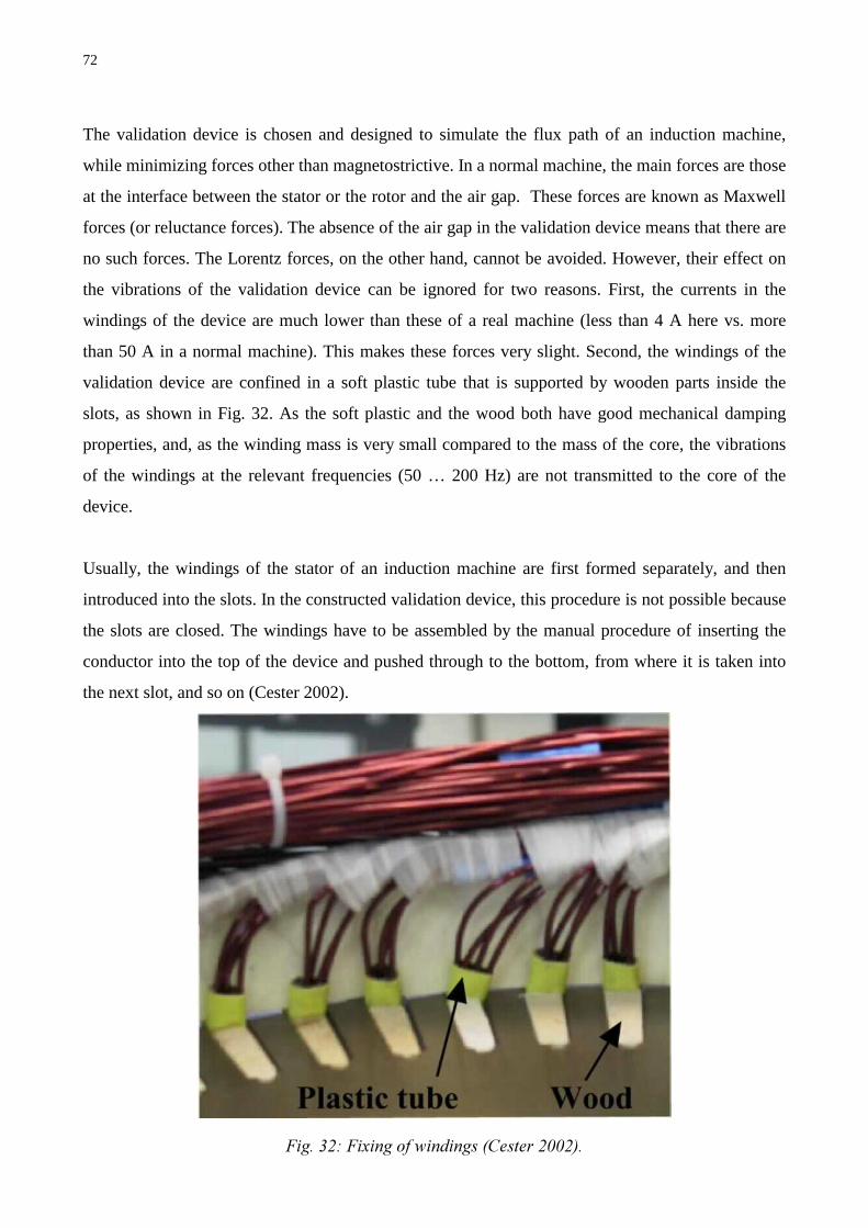
72
The validation device is chosen and designed to simulate the flux path of an induction machine,
while minimizing forces other than magnetostrictive. In a normal machine, the main forces are those
at the interface between the stator or the rotor and the air gap. These forces are known as Maxwell
forces (or reluctance forces). The absence of the air gap in the validation device means that there are
no such forces. The Lorentz forces, on the other hand, cannot be avoided. However, their effect on
the vibrations of the validation device can be ignored for two reasons. First, the currents in the
windings of the device are much lower than these of a real machine (less than 4 A here vs. more
than 50 A in a normal machine). This makes these forces very slight. Second, the windings of the
validation device are confined in a soft plastic tube that is supported by wooden parts inside the
slots, as shown in Fig. 32. As the soft plastic and the wood both have good mechanical damping
properties, and, as the winding mass is very small compared to the mass of the core, the vibrations
of the windings at the relevant frequencies (50 … 200 Hz) are not transmitted to the core of the
device.
Usually, the windings of the stator of an induction machine are first formed separately, and then
introduced into the slots. In the constructed validation device, this procedure is not possible because
the slots are closed. The windings have to be assembled by the manual procedure of inserting the
conductor into the top of the device and pushed through to the bottom, from where it is taken into
the next slot, and so on (Cester 2002).
" !

73
The measurement of the validation device was achieved using conventional measurement devices,
namely, a Wide Band Power Analyser Norma D6100 and a search coil (5 turns, 4100 mm2) around
the yoke of the stator core, for electric and magnetic quantities. A Polytech OFV-302 Single Point
Interferometer laser vibrometer with a standard head was used for the measurement of the velocity
of the outer surface of the device. The measurement set-up is shown in Fig. 33 (Cester 2002).
The velocity measurement was made at different points on the surface of the validation device. The
voltages induced in the search coils, as well as the current and the voltage of the first phase of the
winding, were recorded in real-time. The validation device was supplied with different voltages at
the frequency of 50 Hz; the recording time was 500 ms, which corresponds to 25 periods of the line
voltage. The sampling frequency was 50 kHz, so that a total of 25 000 data points were recorded for
each measured quantity.
The measurement of the validation device began with the measurement of the natural frequencies of
the device and its support. For this purpose, a hammer-test type measurement was made. In this
measurement, the device was exited with a hammer hit and the velocity signal was analysed. The
velocity of the surface of the device is reported in Fig. 34a.
The velocity signal was analysed by DFT in order to determine the natural frequencies of the
supported device. The frequency content of the velocity signal is reported in Fig. 34b. These results
state that, in the measurement of the velocity due to magnetostriction, the frequency components at
about 10 Hz have to be filtered for the signal to be meaningful.
2
The validation device was also simulated with the developed software. The simulations were made
under the same conditions as the measurements. The same voltages were used in the simulations
and the same measured quantities were calculated from the computations results.

74
#$%"&
0.1 0.15 0.2 0.25 0.3 0.35 0.4−1.5
−1
−0.5
0
0.5
1
1.5x 10
−4
Time (s)
Vel
ocity
(m
/s)
0 20 40 60 80 100 120 140 160 180
0
0.5
1
1.5
2
2.5
3
3.5
4
4.5x 10
−5
Frequency (Hz)
Am
plitu
de (
m/s
)
!'!"()&&"(
The results of the measurements were compared to the results of the simulations. These results for a
terminal voltage of 400 V at the frequency of 50 Hz, which correspond to a maximum flux density
in the yoke of the device of about 1.24 T, are presented below. The rest of these results, with
voltages of 300 V and 500 V and a frequency of 50 Hz, are given in Appendix B.
Fig. 35 shows the simulated flux lines in the cross section of the validation device with a line
voltage of 400 V at a frequency of 50 Hz. Fig. 36 shows the calculated magnetostrictive forces at
the last time step. The forces were normalised; the maximum force was 3 580 N/m. The calculated
deformation at the end of the simulation (600 000 times magnified) is shown in Fig. 37. The results
presented in Fig. 35, Fig. 36 and Fig. 37 correspond to the same time step.
(a)
(b)
(c)
(d)
(g)
(f)
(e)
(a) auto-transformer; (b) Norma multi-meter; (c) machine; (d) search coil; (e) laser head;(f) laser controller; (g) PC transient recorder; (h) accelerometer.
(h)
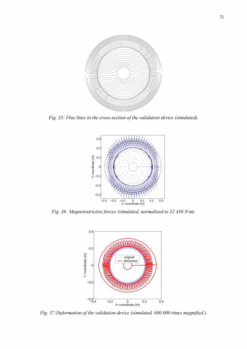
75
*&$"&!
−0.3 −0.2 −0.1 0 0.1 0.2 0.3
−0.3
−0.2
−0.1
0
0.1
0.2
0.3
X−coordinate (m)
Y−
coor
dina
te (
m)
+#",)* -.!
−0.4 −0.2 0 0.2 0.4−0.4
−0.2
0
0.2
0.4
X−coordinate (m)
Y−
coor
dina
te (
m)
originaldeformed
/0""&,+ "!
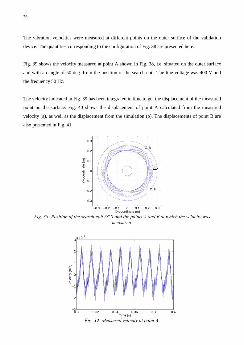
76
The vibration velocities were measured at different points on the outer surface of the validation
device. The quantities corresponding to the configuration of Fig. 38 are presented here.
Fig. 39 shows the velocity measured at point A shown in Fig. 38, i.e. situated on the outer surface
and with an angle of 50 deg. from the position of the search-coil. The line voltage was 400 V and
the frequency 50 Hz.
The velocity indicated in Fig. 39 has been integrated in time to get the displacement of the measured
point on the surface. Fig. 40 shows the displacement of point A calculated from the measured
velocity (a), as well as the displacement from the simulation (b). The displacements of point B are
also presented in Fig. 41.
−0.3 −0.2 −0.1 0 0.1 0.2 0.3
−0.3
−0.2
−0.1
0
0.1
0.2
0.3
X−coordinate (m)
Y−
coor
dina
te (
m)
SC
X A
X B
12"&&$!&%34 &&&
0.3 0.32 0.34 0.36 0.38 0.4−3
−2
−1
0
1
2
3x 10
−5
Time (s)
Vel
ocity
(m
/s)
5#%3

77
0.3 0.32 0.34 0.36 0.38 0.4−4
−3
−2
−1
0
1
2
3
4x 10
−8
Time (s)
Dis
plac
emen
t (m
)
0.1 0.12 0.14 0.16 0.18 0.2
−4
−3
−2
−1
0
1
2
3
4x 10
−8
Dis
plac
emen
t (m
)
Time (s)
!'!) 0%"%3
0.3 0.32 0.34 0.36 0.38 0.4−2
−1.5
−1
−0.5
0
0.5
1
1.5
2
2.5x 10
−8
Time (s)
Dis
plac
emen
t (m
)
0.1 0.12 0.14 0.16 0.18 0.2
−2
−1.5
−1
−0.5
0
0.5
1
1.5
2
2.5x 10
−8
Time (s)
Dis
plac
emen
t (m
)
!'!)0%"%4
0.3 0.32 0.34 0.36 0.38 0.4−15
−10
−5
0
5
10
15
Time (s)
Vol
atge
(V
)
0.1 0.12 0.14 0.16 0.18 0.2
−15
−10
−5
0
5
10
15
Time (s)
Vol
tage
(V
)
!'!)"&&

78
The measured voltage induced in the search coil was compared with the same voltage calculated
from the magnetic field from simulations. These results are shown in Fig. 42.
Some differences between the measured and simulated displacements have to be explained. They
are due to differences between the measured and simulated magnetic quantities. One of the
differences is due to the data on the magnetisation of the iron core. Indeed, the magnetisation curve
used in the simulations is not exactly the measured one, but is linearised at low values of the
magnetic field strength. In this way, the Newton-Raphson iteration is sure to converge and the
software rendered robust. This difference causes higher harmonics to occur in the flux density and
the measured search-coil voltage. The difference between the measured magnetisation data and
those used in simulations can be seen from Fig. 43. For the validation device, this difference is
crucial, since there is no air gap and the device is highly non-linear. However, in normal rotating
electrical machines, the air gap linearises the machine at low values of the magnetic field strength,
so the difference between the measured magnetisation and the used one is not very important.
Moreover, the slope at the origin of the magnetisation curve, measured with an Epstein frame, is
different from the one measured from the constructed validation device. This difference can also be
seen from Fig. 43. The latter magnetisation curve was measured in the following manner. The
windings of the validation device are opened, a current is fed through the shaft of the device and the
induced voltage in the search-coil is measured. From the current and the induced voltage, the
magnetisation curve is plotted. The differences may be due to differences in the material itself; the
one used for the validation device is not necessarily the same as that measured with an Epstein
frame (they are from different lots) or due to mechanical handling in the manufacturing process of
the validation device. The Epstein frame is a standard that does not necessary reproduce the actual
magnetisation curve of the material.
The differences in the wave form of the displacements at point A and B are explained by the
anisotropy of the material. Indeed, the validation device has been constructed so that all the
electrical sheets are in the same direction with regards to materials rolling direction. Although the
material is supposed to be isotropic, a certain amount of anisotropy occurs. The different phases of
the winding are not symmetric and the flux density is different from the calculated one. The
magnetostriction also presents anisotropy, which is not accounted for in the calculations. In normal
electrical machines, this anisotropy is avoided by transposing the electrical sheets.

79
0 200 400 600 800 1000 1200
0
0.2
0.4
0.6
0.8
1
1.2
1.4
1.6
Magnetic field strength H (A/m)
Mag
netic
flux
den
sity
B (
T)
measured with Epstein frameused in simulationsmeasured on the device
)6&&
0.3 0.32 0.34 0.36 0.38 0.4−1.5
−1
−0.5
0
0.5
1
1.5
Time (s)
Flu
x de
nsity
(T
)
0.1 0.12 0.14 0.16 0.18 0.2
−1.5
−1
−0.5
0
0.5
1
1.5
Time (s)
Flu
x de
nsity
(T
)
!'!))&&$
The measured and simulated voltages of the search-coil presented in Fig. 42 were integrated to
obtain the magnetic flux density across the surface of the coil. The measured and simulated flux
densities are shown in Fig. 44. Here also the differences in the wave form of the calculated and
simulated flux density are due to both linearisation and anisotropy.
Finally, the measured and calculated phase currents are presented in Fig. 45. It is clear that, due to
the magnetisation curve used, the measured and simulated phase currents are different. The
maximum value of the measured phase current is larger than the simulated one. This difference does
not affect very much the magnetostriction since the measured and simulated flux densities are
almost the same.

80
0.3 0.32 0.34 0.36 0.38 0.4−2
−1.5
−1
−0.5
0
0.5
1
1.5
2
Time (s)
Pha
se c
urre
nt (
A)
0.1 0.12 0.14 0.16 0.18 0.2
−2
−1.5
−1
−0.5
0
0.5
1
1.5
2
Time (s)
Pha
se c
urre
nt (
A)
!'!)*2&
+
A validation device that simulates the flux path of a rotating electrical machine and minimises all
forces other than magnetostrictive was constructed. The measurements made on this device show
that magnetostriction has a considerable effect on the amplitude of vibrations of rotating electrical
machines.
The differences between the measurements and the simulations are explained. They are caused by
the high non-linearity of the test device and the anisotropy of the iron . In a normal machine, these
differences are expected to be lower due to the linearising effect of the air gap and the skewing of
the iron sheets.
Comparison of the calculated and measured electromagnetic and elastic behaviour of the validation
device shows acceptable agreement and proves the validity of the model presented in this work.
Within the assumptions made on the anisotropy, the correctness of the computation procedures
based on this model is also proved.

81
2
In this chapter, results of computations with different approaches are presented and compared with
each other. Two types of machines are studied; the first one is a relatively large synchronous
generator and the second one is a small-size induction motor. The aim of this chapter is twofold: to
show the computational differences between different approaches and to establish the effect of
magnetostriction and magnetoelastic coupling on the vibrations of rotating electrical machines.
The different approaches used in the following computations are referred to in this work as ($
, , %, %, %, %, & and &
In the quasi-static approach, the effects of mass and damping are ignored in the elastic equations,
while, in the dynamic approach, at least the effect of mass is taken into account. If the damping is
non-zero in the dynamic approach, it is called a damped approach, while a dynamic approach with
zero damping is called an undamped approach. If the geometrical changes are also taken into
account in the solution of the magnetic field, the approach is called coupled, otherwise it is called
uncoupled. Magnetostriction may be taken into account or not in all these approaches.
Magnetostriction can be taken into account in a stress-dependent or stress-independent manner. The
stress-dependent case means that the effect of mechanical stress on the magnetostriction is
accounted for.
All the above-mentioned approaches are computed with the time-stepping method (including the so-
called quasi-static approach). In the coupled quasi-static approach, the geometrical changes are
accounted for only after each step, not during the iteration. In the coupled dynamic approach, these
geometrical changes are accounted for in the iteration process, so that the coordinates of the nodes
can be changed after each iteration.
Discrete Fourier Transform (DFT) was used to analyse the frequency content of the velocity signal
calculated in the simulations. The parameters used with DFT are summarised in Table 1 for each
simulated machine.

82
6'2 &06
Frequency Time-stepsTime step
Per period
Sampling
frequencyResolution
Maximum
Frequency
Synchronous
machine60 Hz 3 000 300 18 kHz 6 Hz 9 000 Hz
Induction
machine and
test device
50 Hz 3 000 300 15 kHz 5 Hz 7 500 Hz
2!
The analysed synchronous machine is a 3.025 MVA generator. This generator is driven by a diesel
motor in a large ship power-plant. The electrical and geometrical parameters of the machine are
given in Appendix C.
Different kinds of magnetoelastic computations were undertaken to check the effect of calculation
methods on the results and the effect of different phenomena on the vibrational behaviour of the
machine. Among the calculated cases, the quasi-static approach, and the dynamic one with different
damping factors, either coupled or not, were applied. The results of these calculations are presented
below.
The calculated deformation of the stator core, at any given time step, and with whichever method,
has the same form, as have the calculated magnetic and magnetostrictive forces; only the absolute
values change. The stator deformation and the radial displacement of a node on the outer surface of
the stator core (point P in Fig. 46a), calculated with the quasi-static approach, are shown in Fig. 46.
The magnetic and magnetostrictive forces are shown in Fig. 47, where the forces have been
normalised. The maximum value of the magnetic forces is 3 023 N/m and that of the
magnetostrictive forces is 8 900 N/m.
The major part of the deformation of the stator core corresponds to a static shrink at spatial mode
zero, on top of which deformations corresponding to different spatial modes are superposed. This
result is in accordance with that obtained from the calculations of the forces with the Maxwell stress
tensor, where the fundamental and the dc components of the radial stress were hundreds of times
bigger than the other ones.

83
−0.6 −0.4 −0.2 0 0.2 0.4 0.6
−0.6
−0.4
−0.2
0
0.2
0.4
0.6
X−coordinate (m)
Y−
coor
dina
te (
m)
originaldeformed
P
0.1 0.12 0.14 0.16 0.18 0.2
−4.5
−4
−3.5x 10
−6
Time (s)
Rad
ial d
ispl
acem
ent (
m)
!" "!'!%"%2)+"%($!
−0.6 −0.4 −0.2 0 0.2 0.4 0.6
−0.6
−0.4
−0.2
0
0.2
0.4
0.6
X−coordinate (m)
Y−
coor
dina
te (
m)
−0.8 −0.6 −0.4 −0.2 0 0.2 0.4 0.6 0.8
−0.8
−0.6
−0.4
−0.2
0
0.2
0.4
0.6
0.8
X−coordinate (m)
Y−
coor
dina
te (
m)
! -.!'!*+ -.!)/#"($!
The magnetic forces are distributed along the nodes at the interface between iron and air or iron and
copper. This phenomenon is due to two facts. On one hand, the major part of the magnetic energy is
stored in the air, while only a small part of it is stored in the iron. On the other hand, the change of
the magnetic energy of one element due to the virtual displacement of nodes inside the iron is
compensated by a change in neighbour elements due to the close values of reluctivity in these
elements. This results in a net nodal force close to zero. Only the great difference between the
reluctivity of iron and that of air (or copper) causes large changes in magnetic energy and large
forces.
The magnetostrictive forces are also distributed on the surface of the stator core, but there are still
some considerable forces inside the iron core. This can be understood by looking at the magnetic
flux path. Due to the magnetostriction, the iron stretches along the flux lines and shrinks in the
orthogonal direction. The flux lines are mostly parallel to the outer surface of the stator core in the

84
yoke and to the surface of the slots in the teeth. Only at the extremities of the electrical poles are
there curvatures of the flux lines. Hence, at these curvatures, the contributions to nodal
magnetostrictive forces from neighbour elements do not compensate each other and a net nodal
force occurs.
The Discrete Fourier Transform was applied to the velocity of the node on the outer surface of the
stator. The frequency content of the velocity is shown in Fig. 48. These results are calculated with
the quasi-static approach and without taking into account the effect of magnetostriction. The results
of calculations with the other approaches and with magnetostriction forces are presented later in this
chapter and compared to the first ones. The frequency content of the velocity calculated without
magnetostriction shows a sharp, high, peak at 1 080 Hz. This result is in accordance with the
measured result, and also with those calculated with the Maxwell stress tensor method. The other
peaks mentioned in the measurements (Chapter 3) are also visible in the frequency contents of the
velocity.
6 4
Calculations with time stepping and the quasi-static elastic approach were undertaken where the
magnetostriction is either taken into account or not. The effect of the displacement field on the FE
magnetic mesh has also been checked within the quasi-static elastic approach. In this last case, the
nodal coordinates are updated after each step, but not within the iterations. The difference in
magnitude of radial displacement of the same node is shown in Fig. 49. A positive difference means
that the amplitude of the first case is bigger than that of the second case.
0 1000 2000 3000 4000 5000 6000 7000 8000 90000
0.5
1
1.5
2x 10
−4
Frequency (Hz)
Am
plitu
de (
m/s
)
)1("&%2)+

85
0.1 0.12 0.14 0.16 0.18 0.2−8
−6
−4
−2
0
2
4
6
8x 10
−10
Time (s)
Diff
eren
ce in
mag
nitu
de (
m)
0.1 0.12 0.14 0.16 0.18 0.2
−7
−6.5
−6
−5.5
−5
−4.5
−4x 10
−7
Time (s)
Diff
eren
ce in
mag
nitu
de (
m)
!%7%'!7)50"""%"%2)+
0 1000 2000 3000 4000 5000 6000 7000 8000 9000−5
−4
−3
−2
−1
0
1
2
3
4x 10
−7
Frequency (Hz)
Am
plitu
de d
iffer
ence
(m/s
)
0 1000 2000 3000 4000 5000 6000 7000 8000 9000−0.5
−0.4
−0.3
−0.2
−0.1
0
0.1
0.2
0.3
Frequency (Hz)
Rel
ativ
e di
ffere
nce
in a
mpl
itude
* 0"""(%7%
0 500 1000 1500−1.5
−1
−0.5
0
0.5
1
1.5
2x 10
−5
Frequency (Hz)
Am
plitu
de d
iffer
ence
(m
/s)
0 500 1000 1500−8
−7
−6
−5
−4
−3
−2
−1
0
1
Frequency (Hz)
Rel
ativ
e di
ffere
nce
in a
mpl
itude
*0"""(7
The magnetostriction causes the amplitude of the dc-component of the mode zero of the radial
displacements to be smaller than those calculated without magnetostriction. Moreover, the
difference is composed of different frequencies. The coupling also changes the vibrations of the

86
stator core in a very complicated manner. These results will be commented on later in this chapter at
the frequency analysis level.
The frequency contents of the velocity as shown in Fig. 48 have also been calculated for both the
above-mentioned cases. The difference between frequency contents calculated with the quasi-static
uncoupled approach and the coupled one, both without magnetostriction, are shown in Fig. 50. The
difference between the uncoupled cases, one without magnetostriction and the other with are shown
in Fig. 51.
The relative differences in the amplitude of velocities between the uncoupled and coupled cases
range from –50 % up to 30 %, depending on the frequency. The most affected frequencies are those
higher than 1 000 Hz. The relative difference is calculated as 1 2
1
−. A negative relative
difference means that the amplitudes of vibration are highest in the second case, while a positive
relative difference means that the amplitudes of vibrations are highest in the first case. Both
negative and positive relative differences occur, as can be seen from Fig. 50. Due to the change in
magnetic field distribution in the core of the machine due to the vibrations of the stator core, there is
an electromagnetoelastic coupling phenomenon that changes the amplitude of vibrations when
compared to the uncoupled case. This phenomenon has been noticed by Arkkio (2001) in a different
approach.
Arkkio (2001) forced the stator of an induction machine to vibrate at given frequencies and modes
and calculated the power that the electromagnetic system absorbs from the vibrating stator core. He
used a relatively large amplitude of vibrations (45 µm, representing 10 % of the radial air gap) in
order to distinguish the damping forces from the radial magnetic forces. The method to compute the
forces was validated by measurements. Both positive and negative damping was found to occur,
depending on the frequency of vibration. The damping in this case was associated with the eddy-
current losses in the windings. The results of the computations presented in this chapter show the
same behaviour, except that here the coupling is bi-directional and the vibrations are not artificially
forced but the effect of the magnetic and/or magnetostrictive forces.
In the text below, the changes in the amplitude of velocities will be referred to as % when the
relative changes are positive and %" when they are negative. This is just an analogy

87
because, in reality, the phenomena occur at the same time. Strictly speaking, these phenomena are
computational damping and amplification, respectively.
The magnetostriction causes the same phenomenon as the coupling, but the relative difference in the
velocity amplitude now ranges from –800 % up to 100 %, depending on the frequency (see Fig. 51).
Some frequencies are damped due to the magnetostriction, including the component at 120 Hz
(25 %). The most damped frequencies are 24 Hz 85 %, 168 Hz 70 %, 390 Hz 60 %, 440 Hz and
456 Hz 55 %. Other frequencies are amplified (e.g. 192 Hz 540 %, 288 Hz 330 %, 432 Hz 785 %
and 1152 Hz 585 %). According to Låftman (1995), magnetostriction can damp vibrations due to
magnetic forces; this can be explained by reference to the damping of some frequencies including
the one at twice the fundamental harmonic. However, this is not the whole truth, since other
frequency components are largely increased.
3!
The dynamic case, which is the main concern of this thesis, has been calculated with different
approaches. First, the undamped dynamic case has been compared with the quasi-static case. The
differences in amplitude of radial displacements of a node on the outer surface of the stator core are
shown in Fig. 52. The differences in frequency contents of the velocities of the same node are
shown in Fig. 53. The effect of inertia (more than 1500 % in some frequency components of the
velocity) is clearly too important to be ignored in time stepping elastic calculations. Moreover, the
components of velocity at high frequency are damped, except at certain values. This damping is
partly due to the calculation method, which includes artificial damping of high frequencies and
makes the method stable (Zienkiewicz 1977).
0.1 0.11 0.12 0.13 0.14 0.15−1
−0.5
0
0.5
1
1.5x 10
−7
Time (s)
Diff
eren
ce in
mag
nitu
de (
m)
*0""%($7

88
0 1000 2000 3000 4000 5000 6000 7000 8000 9000−6
−4
−2
0
2
4
6
8
10x 10
−5
Frequency (Hz)
Am
plitu
de d
iffer
ence
(m/s
)
0 1000 2000 3000 4000 5000 6000 7000 8000 9000−20
−15
−10
−5
0
5
Frequency (Hz)
Rel
ativ
e di
ffere
nce
in a
mpl
itude
*0"""(($7
One problem encountered in the dynamic computation was the effect of structural damping and its
extent in the core of electrical machines. Several computations have been undertaken to check the
effect of damping. In these calculations, the uncoupled approach was used and the magnetostriction
was ignored. The calculated cases with different values of the Rayleigh damping factors α , β and
the corresponding modal damping at 60 and 1 000 Hz are listed in Table 2.
6'%%
α β Modal damping at 60 Hz Modal damping at 1000 Hz
0.00E+00 0.00E+00 0 % 0 %
0.00E+00 1.11E-09 0 % 0.0003 %
0.00E+00 1.11E-08 0.0002 % 0.0035 %
0.00E+00 1.11E-05 0.21 % 3.48 %
0.00E+00 1.11E-04 2.1 % 34.8 %
0.00E+00 1.11E-03 21 % 348 %
0.00E+00 1.11E-02 209 % 3480 %
0.00E+00 1.11E-01 2090 % 34800 %
5.00E+00 1.11E-09 0.66 % 0.04 %
7.00E+00 1.11E-06 0.92 % 0.40 %
4.00E+01 0.00E+00 5.31 % 0.32 %
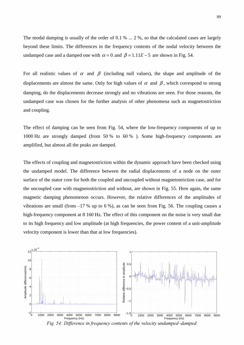
89
The modal damping is usually of the order of 0.1 % ... 2 %, so that the calculated cases are largely
beyond these limits. The differences in the frequency contents of the nodal velocity between the
undamped case and a damped one with 0.α = and 1.11 5β = − are shown in Fig. 54.
For all realistic values of α and β (including null values), the shape and amplitude of the
displacements are almost the same. Only for high values of α and β , which correspond to strong
damping, do the displacements decrease strongly and no vibrations are seen. For those reasons, the
undamped case was chosen for the further analysis of other phenomena such as magnetostriction
and coupling.
The effect of damping can be seen from Fig. 54, where the low-frequency components of up to
1000 Hz are strongly damped (from 50 % to 60 % ). Some high-frequency components are
amplified, but almost all the peaks are damped.
The effects of coupling and magnetostriction within the dynamic approach have been checked using
the undamped model. The difference between the radial displacements of a node on the outer
surface of the stator core for both the coupled and uncoupled without magnetostriction case, and for
the uncoupled case with magnetostriction and without, are shown in Fig. 55. Here again, the same
magnetic damping phenomenon occurs. However, the relative differences of the amplitudes of
vibrations are small (from –17 % up to 6 %), as can be seen from Fig. 56. The coupling causes a
high-frequency component at 8 160 Hz. The effect of this component on the noise is very small due
to its high frequency and low amplitude (at high frequencies, the power content of a unit-amplitude
velocity component is lower than that at low frequencies).
0 1000 2000 3000 4000 5000 6000 7000 8000 9000−2
0
2
4
6
8
10
12x 10
−6
Frequency (Hz)
Am
plitu
de d
iffer
ence
(m/s
)
0 1000 2000 3000 4000 5000 6000 7000 8000 9000
−1.5
−1
−0.5
0
0.5
1
Frequency (Hz)
Rel
ativ
e di
ffere
nce
in a
mpl
itude
*)0"""("&%7%

90
The effect of coupling and magnetostriction on the frequency contents of the velocity of the same
node can be seen from Fig. 56 as the difference between the coupled and uncoupled cases, both
without magnetostriction, and from Fig. 57 as the difference between the uncoupled cases, either
with or without magnetostriction.
The effect of magnetostriction is very considerable compared with that of coupling (from –800 %
up to 100 %). The magnetostriction damps some frequency components including the one at
120 Hz, which is usually attributed to magnetostriction, (25 %) while it increases others. The effect
of magnetostriction can be ignored for frequencies higher than 1 500 Hz.
0.1 0.12 0.14 0.16 0.18 0.2−2
−1
0
1
2
3
4
5
6
7x 10
−10
Time (s)
Diff
eren
ce in
mag
nitu
de (
m)
0.1 0.12 0.14 0.16 0.18 0.2
−7
−6.5
−6
−5.5
−5
−4.5
−4x 10
−7
Time (s)
Diff
eren
ce in
mag
nitu
de (
m)
!%7%'!7**0""%
0 1000 2000 3000 4000 5000 6000 7000 8000 9000−3.5
−3
−2.5
−2
−1.5
−1
−0.5
0
0.5x 10
−7
Frequency (Hz)
Am
plitu
de d
iffer
ence
(m/s
)
0 1000 2000 3000 4000 5000 6000 7000 8000 9000−0.2
−0.15
−0.1
−0.05
0
0.05
0.1
0.15
Frequency (Hz)
Rel
ativ
e di
ffere
nce
in a
mpl
itude
*+0"""(%7%
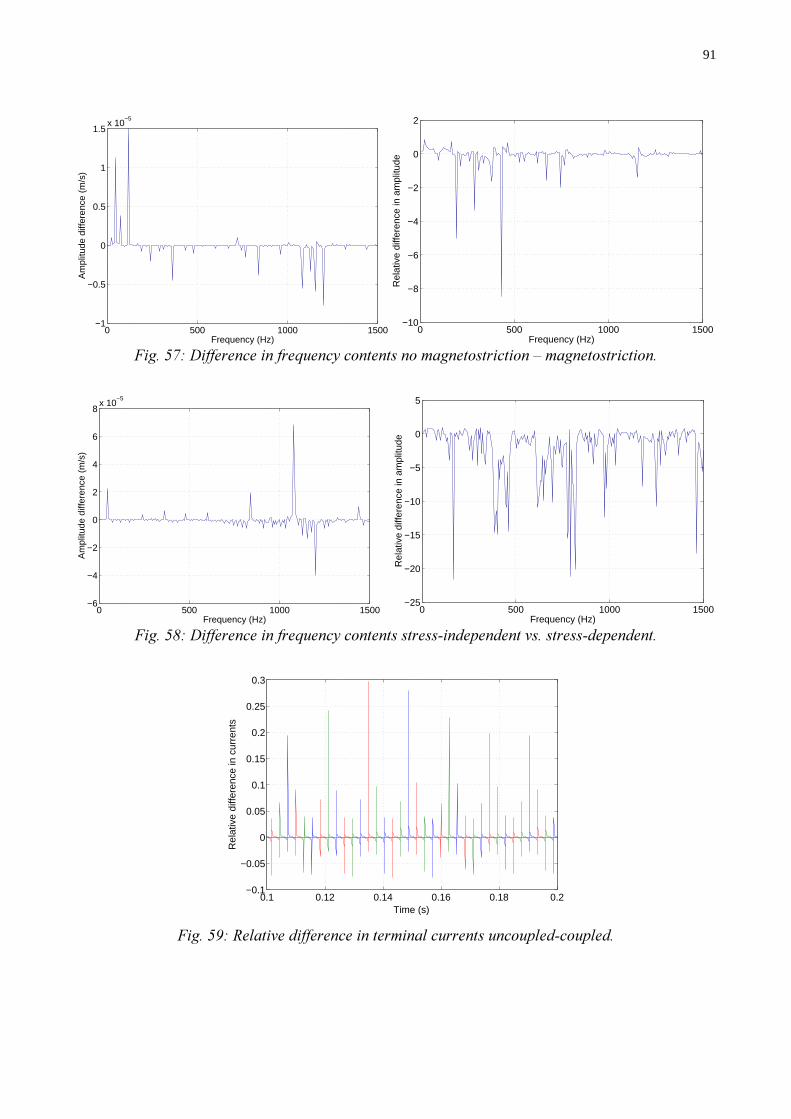
91
0 500 1000 1500−1
−0.5
0
0.5
1
1.5x 10
−5
Frequency (Hz)
Am
plitu
de d
iffer
ence
(m
/s)
0 500 1000 1500−10
−8
−6
−4
−2
0
2
Frequency (Hz)
Rel
ativ
e di
ffere
nce
in a
mpl
itude
*/0"""(7
0 500 1000 1500−6
−4
−2
0
2
4
6
8x 10
−5
Frequency (Hz)
Am
plitu
de d
iffer
ence
(m
/s)
0 500 1000 1500
−25
−20
−15
−10
−5
0
5
Frequency (Hz)
Rel
ativ
e di
ffere
nce
in a
mpl
itude
*10"""($%$%
0.1 0.12 0.14 0.16 0.18 0.2−0.1
−0.05
0
0.05
0.1
0.15
0.2
0.25
0.3
Rel
ativ
e di
ffere
nce
in c
urre
nts
Time (s)
*58""%$%

92
0.1 0.12 0.14 0.16 0.18 0.2−2
−1
0
1
2
x 10−4
Time (s)
Rel
ativ
e di
ffere
nce
in to
rque
+ 8""(%$%
The effect of stress on magnetostriction has also been checked. The differences in the frequency
contents of the velocity of the same node on the outer surface of the stator core are presented in Fig.
58. Here the stress-dependency of the magnetostriction increases almost all the frequency
components. Some of them are increased by up to 2 000 %. However, the high frequencies are
increased much more (not shown in Fig. 58). This increase is not correct, being due to the
inaccuracy of the linear triangular elastic elements combined with large values of the magnetic
forces. It is also partly due to the effect of magnetostrictive stress on the calculated mechanical
stress. Indeed, modelling the magnetostriction with equivalent forces causes mechanical stresses to
occur in the material although the structure modelled is free to stretch or shrink. This phenomenon
has been explained in Chapter 2.
Fig. 59 shows the relative difference in terminal currents between the cases uncoupled and coupled
XQFRXSOHG FRXSOHG
XQFRXSOHG
9 9
9
−
. Sharp peaks of up to 25 % of the terminal current are calculated when the
coupling is taken into account. This difference in current is not necessary visible in the Real Mean
Square values of the current since it can be a result of a phase shift only. The magnetoelastic
coupling does not have a major effect on the calculated torque, as can be seen from Fig. 60, where
the relative difference in electromagnetic torque XQFRXSOHG FRXSOHG
XQFRXSOHG
6 6
6
−
is shown (less than 2E-4 %).
/
The analysed induction machine is a small-size 37 kW motor, the parameters of which are given in
appendix D.
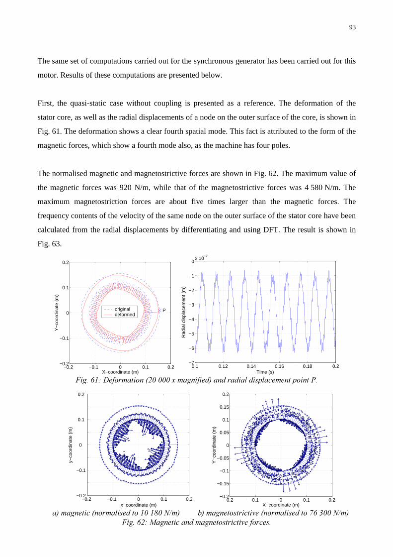
93
The same set of computations carried out for the synchronous generator has been carried out for this
motor. Results of these computations are presented below.
First, the quasi-static case without coupling is presented as a reference. The deformation of the
stator core, as well as the radial displacements of a node on the outer surface of the core, is shown in
Fig. 61. The deformation shows a clear fourth spatial mode. This fact is attributed to the form of the
magnetic forces, which show a fourth mode also, as the machine has four poles.
The normalised magnetic and magnetostrictive forces are shown in Fig. 62. The maximum value of
the magnetic forces was 920 N/m, while that of the magnetostrictive forces was 4 580 N/m. The
maximum magnetostriction forces are about five times larger than the magnetic forces. The
frequency contents of the velocity of the same node on the outer surface of the stator core have been
calculated from the radial displacements by differentiating and using DFT. The result is shown in
Fig. 63.
−0.2 −0.1 0 0.1 0.2−0.2
−0.1
0
0.1
0.2
X−coordinate (m)
Y−
coor
dina
te (
m)
originaldeformed
P
0.1 0.12 0.14 0.16 0.18 0.2
−7
−6
−5
−4
−3
−2
−1
0x 10
−7
Time (s)
Rad
ial d
ispl
acem
ent (
m)
+0" "!%%2
−0.2 −0.1 0 0.1 0.2−0.2
−0.1
0
0.1
0.2
x−coordinate (m)
y−co
ordi
nate
(m
)
−0.2 −0.1 0 0.1 0.2
−0.2
−0.15
−0.1
−0.05
0
0.05
0.1
0.15
0.2
X−coordinate (m)
Y−
coor
dina
te (
m)
! 1 -.!'!/+ -.!+#"
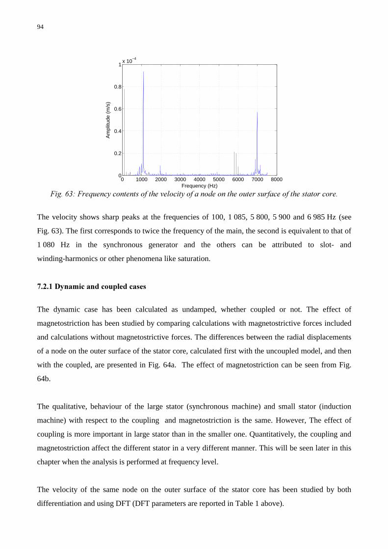
94
0 1000 2000 3000 4000 5000 6000 7000 80000
0.2
0.4
0.6
0.8
1x 10
−4
Frequency (Hz)
Am
plitu
de (
m/s
)
+("&"&""&
The velocity shows sharp peaks at the frequencies of 100, 1 085, 5 800, 5 900 and 6 985 Hz (see
Fig. 63). The first corresponds to twice the frequency of the main, the second is equivalent to that of
1 080 Hz in the synchronous generator and the others can be attributed to slot- and
winding-harmonics or other phenomena like saturation.
3!
The dynamic case has been calculated as undamped, whether coupled or not. The effect of
magnetostriction has been studied by comparing calculations with magnetostrictive forces included
and calculations without magnetostrictive forces. The differences between the radial displacements
of a node on the outer surface of the stator core, calculated first with the uncoupled model, and then
with the coupled, are presented in Fig. 64a. The effect of magnetostriction can be seen from Fig.
64b.
The qualitative, behaviour of the large stator (synchronous machine) and small stator (induction
machine) with respect to the coupling and magnetostriction is the same. However, The effect of
coupling is more important in large stator than in the smaller one. Quantitatively, the coupling and
magnetostriction affect the different stator in a very different manner. This will be seen later in this
chapter when the analysis is performed at frequency level.
The velocity of the same node on the outer surface of the stator core has been studied by both
differentiation and using DFT (DFT parameters are reported in Table 1 above).

95
The differences in the frequency contents for the quasi-static – dynamic, uncoupled – coupled
(without magnetostriction) and no magnetostriction – magnetostriction (uncoupled) cases are shown
respectively in Fig. 65, Fig. 66 and Fig. 67.
It is clear here again that the dynamic nature of the stator vibrations has to be taken into account for
more accurate evaluations of these vibrations. The relative difference in the amplitudes of velocities
calculated with the quasi-static elastic approach and the dynamic one is from –500 % up to 100 %;
almost all the frequencies are affected (see Fig. 65). Due to the higher mechanical stiffness of the
small stator, the high frequencies are much affect than the low one. This was not the case for the
large stator of the synchronous machine. This latter one is mechanically less stiff, which explains its
behaviour in the calculations with coupled approach.
0.1 0.12 0.14 0.16 0.18 0.2−2
−1.5
−1
−0.5
0x 10
−11
Time (s)
Diff
eren
ce in
mag
nitu
de (
m)
0.1 0.12 0.14 0.16 0.18 0.2−1.7
−1.6
−1.5
−1.4
−1.3
−1.2x 10
−7
Time (s)
Diff
eren
ce in
mag
nitu
de (
m)
!%7%'!7+)0""%
0 1000 2000 3000 4000 5000 6000 7000 8000−0.5
0
0.5
1
1.5
2
2.5
3x 10
−5
Frequency (Hz)
Am
plitu
de d
iffer
ence
(m/s
)
0 1000 2000 3000 4000 5000 6000 7000 8000−6
−5
−4
−3
−2
−1
0
1
Frequency (Hz)
Rel
ativ
e di
ffere
nce
in a
mpl
itude
+*0"""(($7

96
0 1000 2000 3000 4000 5000 6000 7000 8000−2
0
2
4
6
8
10
12x 10
−9
Frequency (Hz)
Am
plitu
de d
iffer
ence
(m/s
)
0 1000 2000 3000 4000 5000 6000 7000 8000−5
−4
−3
−2
−1
0
1
2
3x 10
−3
Frequency (Hz)
Rel
ativ
e di
ffere
nce
in a
mpl
itude
++0"""(%7%
0 500 1000 1500 2000−2
−1
0
1
2
3
4
5
6x 10
−6
Frequency (Hz)
Am
plitu
de d
iffer
ence
(m
/s)
0 500 1000 1500 2000−10
−8
−6
−4
−2
0
2
Frequency (Hz)
Rel
ativ
e di
ffere
nce
in a
mpl
itude
+/0"""(7
The effect of coupling on the stator vibration of the small induction machine is almost non-existent
(0.5 % at its maximum see Fig. 66). This is because the small stator is mechanically stiffer than the
large one. The displacements are very small and their effect on the magnetic calculation is
negligible.
On one hand, the magnetostriction in the case of the small stator damps some frequency
components of the velocity, e.g., those at 25 Hz (70 %), 100 Hz (7 %), 280 Hz (45 %) and 1190 Hz
(80 %). On the other hand, some frequency components are much more increased, like the ones at
40, 50 and 60 Hz (respectively 400, 320 and 280 %) also the one at 490 Hz (840 %) among others
(see Fig. 67). The argument in Låftman (1995), according to which the magnetostriction might
damp the vibrations due to magnetic forces, can only be partly validated with these results.
Furthermore, the increase in the frequency components at 40, 50, 60 and 490 Hz cannot be
explained by such simple reasoning.

97
The results presented by Delaere (2002), namely that the magnetostrictive forces can be ignored and
that they do not affect the noise and vibrations of rotating electrical machines, contradict the results
presented in this chapter. In Delaere (2002), the magnetostrictive forces are calculated in an
equivalent manner as it is done in this work. However, the data on the magnetostriction was missing
and a simple function of the square of the flux density was used. The only results from the literature
that agree somehow with the presented calculations are those presented by Witczak (1996). He
calculated large magnetostrictive forces in an induction machine.
In Fig. 68, the stresses in the direction parallel to that of the flux density vector at each element
are plotted. These are stresses calculated in the dynamic case without taking into account the effect
either of magnetostriction or of the magnetoelastic coupling. The stresses vary from –1 to 1.5 MPa.
Looking at the measurement results of magnetostriction, it becomes clear that the effect of stress on
magnetostriction has to be taken into account when evaluating magnetostriction forces.
Fig. 69 shows the differences in the stress component in the direction parallel to that of the flux
density vector. Most of the differences are between –800 and 200 kPa. This result explains why the
integration, with respect to the flux density, in the calculation of the magnetic energy and the
magnetic and magnetostriction forces are made at constant stress. However, the stress induced by
magnetostriction is large enough to cause some calculation error. This problem has been
experienced when the calculations with both magnetoelastic coupling and stress-dependent
magnetostriction were tried. The Newton iterations did not converge and the combined effect of
magnetostriction and magnetoelastic coupling could not be established, except in the case of stress-
independent magnetostriction.
0 500 1000 1500 2000−1
−0.5
0
0.5
1
1.5x 10
6
Element number
Str
ess
(Pa)
+1%"%&
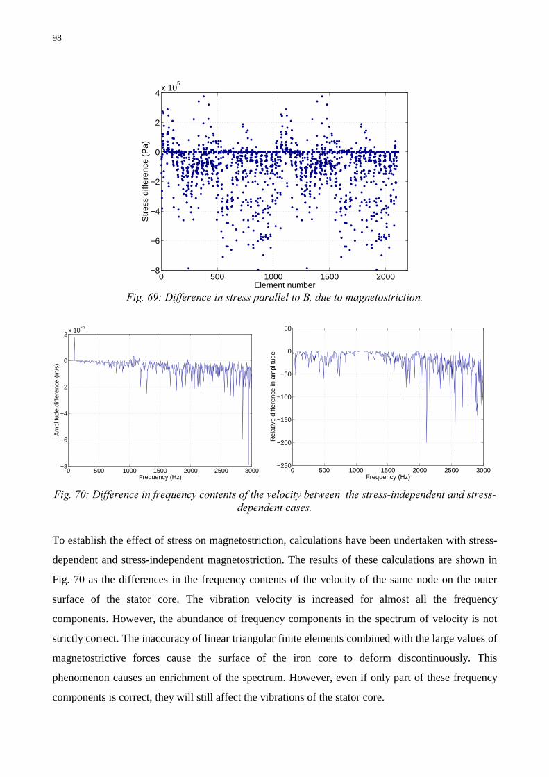
98
0 500 1000 1500 2000−8
−6
−4
−2
0
2
4x 10
5
Element number
Str
ess
diffe
renc
e (P
a)
+50""%4,
0 500 1000 1500 2000 2500 3000−8
−6
−4
−2
0
2x 10
−5
Frequency (Hz)
Am
plitu
de d
iffer
ence
(m
/s)
0 500 1000 1500 2000 2500 3000
−250
−200
−150
−100
−50
0
50
Frequency (Hz)
Rel
ativ
e di
ffere
nce
in a
mpl
itude
/ 0"""("&' &$%$%
To establish the effect of stress on magnetostriction, calculations have been undertaken with stress-
dependent and stress-independent magnetostriction. The results of these calculations are shown in
Fig. 70 as the differences in the frequency contents of the velocity of the same node on the outer
surface of the stator core. The vibration velocity is increased for almost all the frequency
components. However, the abundance of frequency components in the spectrum of velocity is not
strictly correct. The inaccuracy of linear triangular finite elements combined with the large values of
magnetostrictive forces cause the surface of the iron core to deform discontinuously. This
phenomenon causes an enrichment of the spectrum. However, even if only part of these frequency
components is correct, they will still affect the vibrations of the stator core.
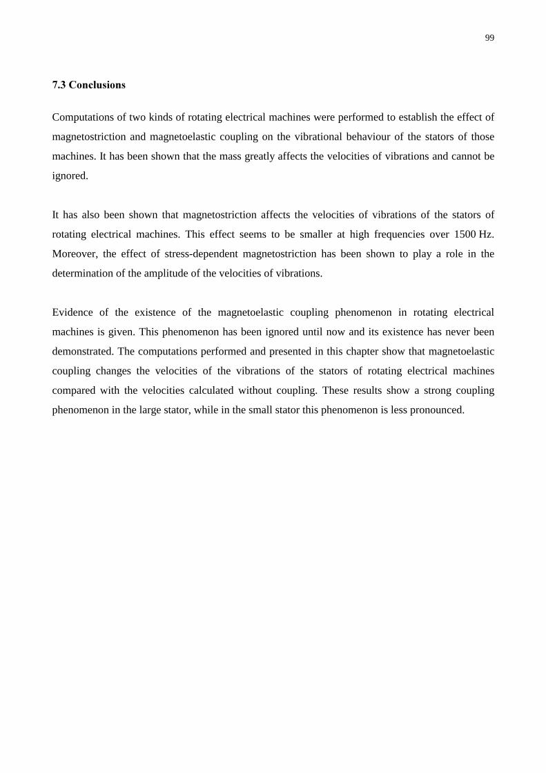
99
+
Computations of two kinds of rotating electrical machines were performed to establish the effect of
magnetostriction and magnetoelastic coupling on the vibrational behaviour of the stators of those
machines. It has been shown that the mass greatly affects the velocities of vibrations and cannot be
ignored.
It has also been shown that magnetostriction affects the velocities of vibrations of the stators of
rotating electrical machines. This effect seems to be smaller at high frequencies over 1500 Hz.
Moreover, the effect of stress-dependent magnetostriction has been shown to play a role in the
determination of the amplitude of the velocities of vibrations.
Evidence of the existence of the magnetoelastic coupling phenomenon in rotating electrical
machines is given. This phenomenon has been ignored until now and its existence has never been
demonstrated. The computations performed and presented in this chapter show that magnetoelastic
coupling changes the velocities of the vibrations of the stators of rotating electrical machines
compared with the velocities calculated without coupling. These results show a strong coupling
phenomenon in the large stator, while in the small stator this phenomenon is less pronounced.

100
*3
The aim of this chapter is to summarise and discuss the results obtained in this work. Some
computational aspects of the results, such as computation time and accuracy, are also discussed.
Suggestions as to how this work might be developed in the future, and possible issues relating to its
future applications, are also presented.
*/ 1
The updated literature review undertaken during the years of this study shows that the problem of
magnetostriction in electrical machines is still a matter of controversy. Many researchers tried, and
still try, to address the question of the nature of the effects of magnetostriction on the vibrations and
noise of rotating electrical machines. The model used for magnetostriction varies from one author to
another, and the differences between the results remain too large to allow definitive answers.
Although the magnetostriction phenomenon by itself is well understood, a major difference between
the so-called magnetostrictive forces and magnetic or reluctance forces should be emphasised. This
difference resides in the effect of these forces on elastic structures. While the magnetic forces act
mainly at interfaces between different materials (mostly iron-air interfaces) causing rigid body
displacements and elastic deformations of the structures, the magnetostrictive forces act at different
parts of the iron, only causing deformations other than rigid-body ones, and tending to stretch or
shrink the iron without any major effect on the structure itself. This difference makes the effects of
magnetic and magnetostrictive forces on a stator of electrical machines very different from one
another. The magnetic forces act on an elastic structure with relatively low stiffness, while the
magnetostrictive forces act on the material itself, which is very stiff. Although the magnetostriction
forces are many times larger than the magnetic forces, their effect on the vibrations of the structures
is, except at some frequencies, less important than that of the magnetic forces.
The separation of magnetic forces into the forces traditionally called magnetic (or reluctance) forces
and magnetostriction forces is shown in the derivation of magnetic forces from the principle of
virtual work. In this method, the magnetic forces are composed of different terms.
If the stress dependence of the magnetisation is not taken into account, the non-zero terms are
demonstrated to give the same total force as the Maxwell stress tensor method. However, while the
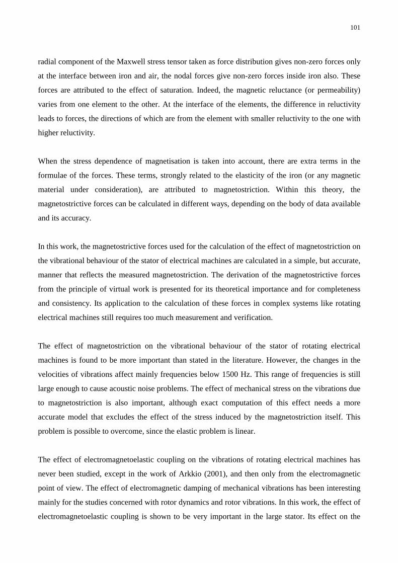
101
radial component of the Maxwell stress tensor taken as force distribution gives non-zero forces only
at the interface between iron and air, the nodal forces give non-zero forces inside iron also. These
forces are attributed to the effect of saturation. Indeed, the magnetic reluctance (or permeability)
varies from one element to the other. At the interface of the elements, the difference in reluctivity
leads to forces, the directions of which are from the element with smaller reluctivity to the one with
higher reluctivity.
When the stress dependence of magnetisation is taken into account, there are extra terms in the
formulae of the forces. These terms, strongly related to the elasticity of the iron (or any magnetic
material under consideration), are attributed to magnetostriction. Within this theory, the
magnetostrictive forces can be calculated in different ways, depending on the body of data available
and its accuracy.
In this work, the magnetostrictive forces used for the calculation of the effect of magnetostriction on
the vibrational behaviour of the stator of electrical machines are calculated in a simple, but accurate,
manner that reflects the measured magnetostriction. The derivation of the magnetostrictive forces
from the principle of virtual work is presented for its theoretical importance and for completeness
and consistency. Its application to the calculation of these forces in complex systems like rotating
electrical machines still requires too much measurement and verification.
The effect of magnetostriction on the vibrational behaviour of the stator of rotating electrical
machines is found to be more important than stated in the literature. However, the changes in the
velocities of vibrations affect mainly frequencies below 1500 Hz. This range of frequencies is still
large enough to cause acoustic noise problems. The effect of mechanical stress on the vibrations due
to magnetostriction is also important, although exact computation of this effect needs a more
accurate model that excludes the effect of the stress induced by the magnetostriction itself. This
problem is possible to overcome, since the elastic problem is linear.
The effect of electromagnetoelastic coupling on the vibrations of rotating electrical machines has
never been studied, except in the work of Arkkio (2001), and then only from the electromagnetic
point of view. The effect of electromagnetic damping of mechanical vibrations has been interesting
mainly for the studies concerned with rotor dynamics and rotor vibrations. In this work, the effect of
electromagnetoelastic coupling is shown to be very important in the large stator. Its effect on the

102
vibrational behaviour of small-size stators is not that important. This result is logical, since the
elastic displacements in large stators are much larger than those in small-size stators.
One aspect of the electromagnetoelastic coupling that has not been studied in this work is the
change of magnetisation with respect to mechanical stress. This problem has been disregarded for
three reasons: the low level of stress in the stator core, the lack in the knowledge of the effect of
multidirectional stress on the magnetisation and the lack of time.
The main achievements of this work are the development of the theory and formula relating to
magnetoelastic coupling within time stepping FE analysis and the building of the required
simulation tools. The measurement of magnetisation and magnetostriction under externally applied
mechanical stress is also an achievement, which produced results that have many applications,
either of theoretical interest, like the determination of magnetoelastic coupling constants, or of
computational interest, as in this work. Last but not least, the simulations of the two kinds of
machines and the results obtained from these simulations are very important for those designers
concerned with the problems of the vibrations and noise of rotating electrical machines.
* ( !
The accuracy of the developed model and that of the computation are difficult to evaluate. However,
some considerations have to be mentioned. First, the developed tools are based on linear triangular
finite elements, the accuracy of which is not the best possible. The development of the formula for
elements of a higher order is a task that can be better addressed in the next section (8.3 Future
work). However, before doing so, an estimate of the computation time with second- or third-order
elements is needed. Second, the magnetic field solution is based on the φ− formulation of the
magnetic field. In this formulation, the magnetic flux density is solved accurately at element level,
but the magnetic field strength is not. The continuity of the tangential component of the magnetic
field strength is not guaranteed within this formulation. This discontinuity results in inaccuracies of
both the magnetic vector potential and the magnetic forces. These phenomena are important in the
iron core, but as we have seen, the forces in the iron core are very small compared with those on its
surface.

103
The effect of magnetostrictive stress on the total mechanical stress in iron elements also decreases
the accuracy of the calculation of magnetostrictive forces when the stress-dependency of the
magnetostriction is taken into account.
These remarks, and the measurements made on the validation device, allow us to say that the
accuracy of the method, as well as that of the computations, are sufficiently accurate to allow us to
draw the conclusions presented in this work. The only way of estimating the accuracy of the
computations would be by complicated measurement of the vibrations of the computed machines as
well as the magnetic flux density in the core of these machines through search coils. This
measurement has not been performed on the simulated machines (synchronous and induction).
The accuracy of the measured data, on the other hand, can be considered as good. According to the
specifications of the measurement devices used, and within the range of measured values, the error
in measurements is less than 5 %. However, the measured values are hysteresis loops of either
magnetisation or magnetostriction. These loops needed filtering and averaging to get them into a
form suitable for the computations. As a result, a rough estimate of the error on these values is about
10 %.
The error on the measurement made on the validation device is estimated to be about 10 %, based
again on the specifications of instruments used for these measurements.
The computations were performed on different platforms. A total of 4000 time steps with 300 steps
per period of the line voltage was computed in each case. Each time step took five or six iterations,
depending on whether the problem was coupled or not. On a Sun Microsystems Blade 100
workstation with an UltraSPARC-IIe processor having a clock frequency of 500 MHz, the total
computation time was 10h 15min for an uncoupled dynamic case and 18h 16min for the coupled
one. This is already a huge computation time, and the idea of second- or higher-order finite elements
does not sound reasonable at least at this computational speed.
However, the tools developed here are for research or special analysis purposes. The program code
is not optimised and a possible lowering of the number of equations by using geometrical and
electrical symmetry of the machines was not used. Taking advantage of these technical
considerations might reduce the computation time.

104
*"1
The path from vibrations to the noise level of rotating electrical machines is long and complex.
Different aspects of the problem have to be studied. Among these aspects, we can mention here the
structure of the machine mounting, the mechanism of vibration transfer from the stator core to the
structure around it, the pre-stress of the stator core (in some induction machines the stator core is
under pre-stress from the surrounding frame) and the radiation of noise by the vibrating components
of the mounted machine. All these aspects require special studies that are beyond the scope of this
thesis; nevertheless, the study of aspects such as these is necessary if a better understanding and
quantitative establishment of the problem of noise from rotating electrical machines is to be gained.
The results and the tools built in this work give a good background for further studies. These tools
can also be used to study more complex phenomena like the effect of stress on magnetisation.
However, logically, the next step in this work is the systematic simulation of different types and
sizes of electrical machines and the use of statistical analysis of the results to formulate general
rules for the use of magnetostriction and electromagnetoelastic coupling to build and design less
noisy rotating electrical machines.
Last and not least, The effect of mechanical stress on the iron losses has not been studied in this
work. The mechanical stress is known to increase the magnetic losses in iron sheets. This is also a
subject than needs more work an deep studies to establish how the losses are changed and whether it
is possible to reduce them by any means.

105
((78
The main parameters of the validation device are listed below. Figure A1 shows the geometry of the
cross section of the device (only a quarter is shown), while Fig. A2 shows the geometry of a slot.
Table A1 gives the electric parameters of the device and its windings. Table A2 gives the
dimensions of the slot and Table A3 those of the device.
6'3%"&Number of poles 2
Number of phases 3
Number of parallel paths 1
Number of conductors in a stator slot 8
Number of layers of the stator winding 2
Coil pitch in slot pitches 30
3:"&
6'3Slot data [mm] 6'3"&H1 54 Stator data [mm]H2 44 Inner diameter DIN 410H3 3 Outer diameter DEXT 600B1 4 Shaft diameter DS 100B2 12 Height of stator yoke HSY 41B3 8 Length of stator core Th 100
3:"&
H2
H4H3
B2
B1
B3
H1
DIN
DS
DEXT
HSY
DES
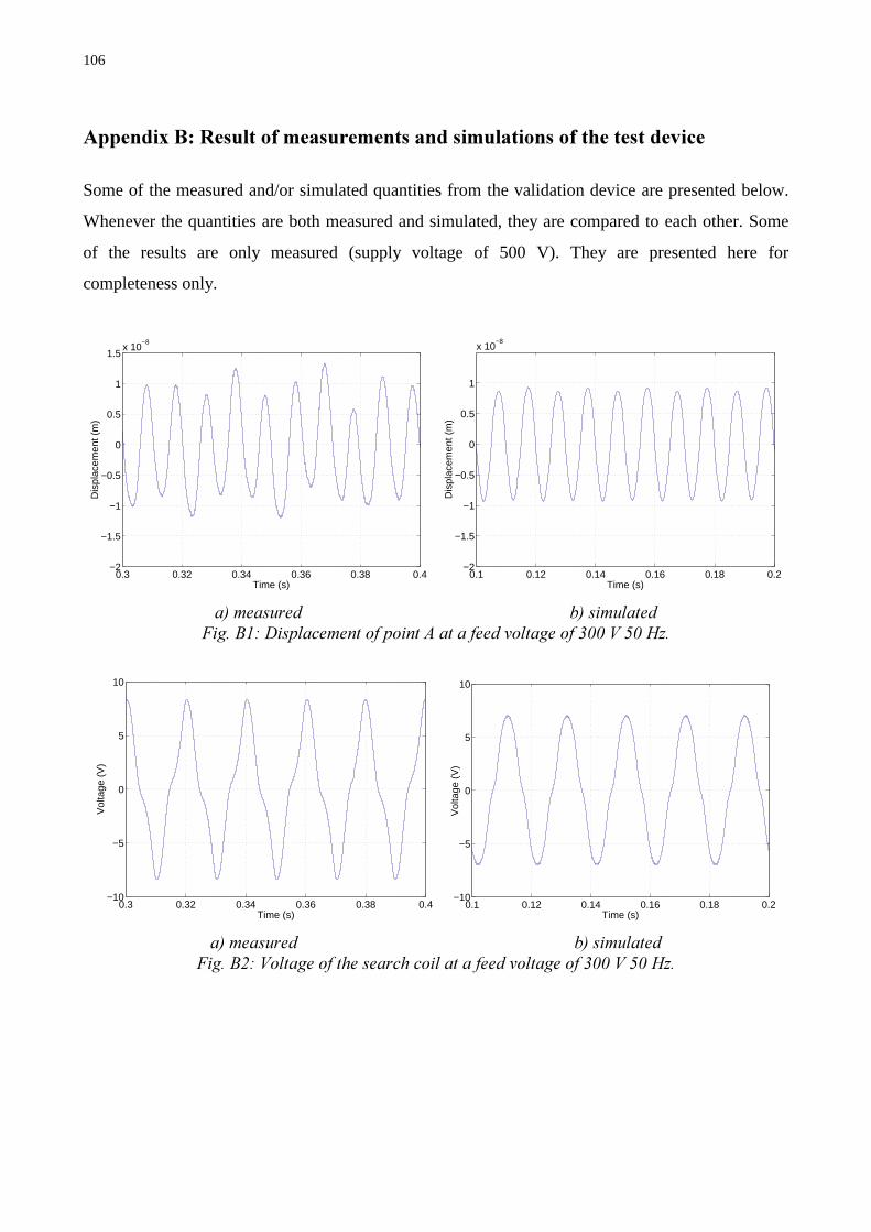
106
(.79
Some of the measured and/or simulated quantities from the validation device are presented below.
Whenever the quantities are both measured and simulated, they are compared to each other. Some
of the results are only measured (supply voltage of 500 V). They are presented here for
completeness only.
0.3 0.32 0.34 0.36 0.38 0.4−2
−1.5
−1
−0.5
0
0.5
1
1.5x 10
−8
Time (s)
Dis
plac
emen
t (m
)
0.1 0.12 0.14 0.16 0.18 0.2
−2
−1.5
−1
−0.5
0
0.5
1
x 10−8
Time (s)
Dis
plac
emen
t (m
)
!'!40%"%3"" * ;
0.3 0.32 0.34 0.36 0.38 0.4−10
−5
0
5
10
Time (s)
Vol
tage
(V
)
0.1 0.12 0.14 0.16 0.18 0.2
−10
−5
0
5
10
Time (s)
Vol
tage
(V
)
!'!4"&&"" * ;
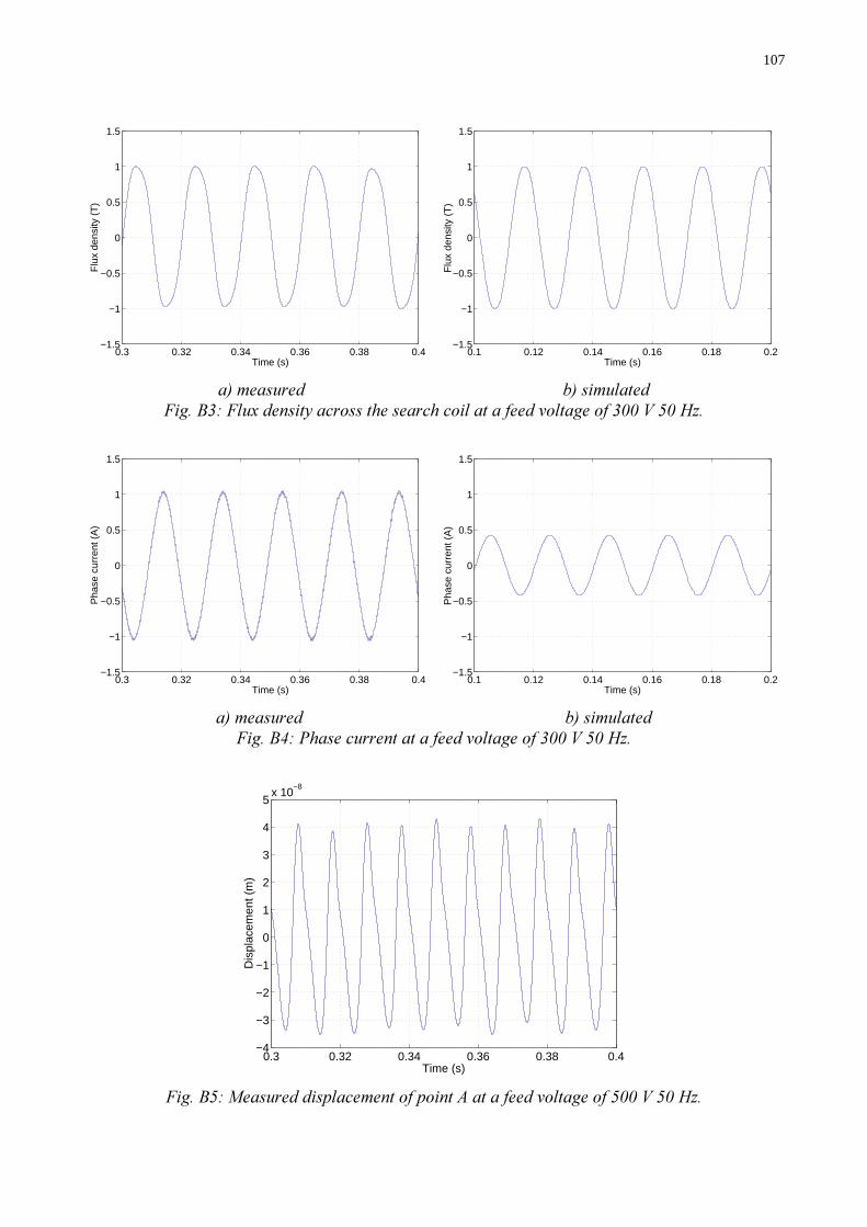
107
0.3 0.32 0.34 0.36 0.38 0.4−1.5
−1
−0.5
0
0.5
1
1.5
Time (s)
Flu
x de
nsity
(T
)
0.1 0.12 0.14 0.16 0.18 0.2
−1.5
−1
−0.5
0
0.5
1
1.5
Time (s)
Flu
x de
nsity
(T
)
!'!4&&"" * ;
0.3 0.32 0.34 0.36 0.38 0.4−1.5
−1
−0.5
0
0.5
1
1.5
Time (s)
Pha
se c
urre
nt (
A)
0.1 0.12 0.14 0.16 0.18 0.2
−1.5
−1
−0.5
0
0.5
1
1.5
Time (s)
Pha
se c
urre
nt (
A)
!'!4)2&"" * ;
0.3 0.32 0.34 0.36 0.38 0.4−4
−3
−2
−1
0
1
2
3
4
5x 10
−8
Time (s)
Dis
plac
emen
t (m
)
4*#%"%3""* * ;

108
0.3 0.32 0.34 0.36 0.38 0.4−20
−15
−10
−5
0
5
10
15
20
Time (s)
Vol
tage
(V
)
0.3 0.32 0.34 0.36 0.38 0.4
−1.5
−1
−0.5
0
0.5
1
1.5
Time (s)
Flu
x de
nsity
(T
)
!'!"4+#"&&"""*
* ;
0.3 0.32 0.34 0.36 0.38 0.4−4
−3
−2
−1
0
1
2
3
4
Time (s)
Pha
se c
urre
nt (
A)
4/#%&""* * ;

109
(+78 !!
The rated values and geometry of the synchronous machine simulated and analysed in Chapter 7 are
given in table C1.
The synchronous machine was simulated at the rated power. The field current was 100 A and the
terminal current 300 A. The power factor was 0.80 and the displacement factor 0.80 capacitive. The
shaft power was 2.78 MW.
6'8"&&&Rated power 3,025 MVA Number of stator slots 96
Rated voltage 6600 V Stack length 1200 mm
Frequency 60 Hz Stator outer diameter 1200 mm
Number of phases 3 Stator inner diameter 950 mm
Number of poles 10 Damping bars/pole 4
Power factor 0.80 Cap.
130
195
200
100
52
14
18
59.5
R115
R470
:!"&&&

110
(378 !
The rated values and geometry of the induction machine simulated and analysed in Chapter 7 are
given in table D1.
The induction machine was simulated at the rated power. The terminal current was 68.2 A, shaft
power 36.2 kW and the power factor 0.83.
6'08"&&Rated power 37 kW Stator outer diameter 310 mm
Rated voltage 380 V Stator inner diameter 200 mm
Connection Star Stack length 289 mm
Slip 1.7 % Number of stator slots 48
Frequency 50 Hz Rotor outer diameter 198.4 mm
Number of phases 3 Rotor inner diameter 70 mm
Number of poles 4 Number of rotor slots 40
6.5
3.5
6
2.5
5.85
17.8
15.4
6
17.5
23.9
8.8
0:!"&&

111
9
Arkkio, A. 1987, “Analysis of Induction Motors Based on the Numerical Solution of the Magnetic
Field and Circuit Equations”, doctoral thesis, Acta Polytechnica Scandinavica, Electrical
Engineering Series No. 59, 97 p. <http://lib.hut.fi/Diss/198X/isbn951226076X/>
Arkkio, A. 1995, “Unbalanced Magnetic Pull in a Four-Pole Induction Motor with an Odd Number
of Rotor Slots”, Proceedings of CICEM'95, Hangzhou, 31 Aug. - 2 Sept. 1995, China, pp. 343–348.
Arkkio, A. 2001, “Electromagnetic Damping of Stator Vibrations in a Cage Induction Motor”, VTT
SYMPOSIUM 209, Espoo 2001, pp. 25–44.
Bath, K. J. 1982, “Finite Element Procedure in Engineering Analysis”, Prentice-Hall International,
New Jersey, 1982, 735 p.
Belahcen, A., Arkkio, A., Klinge, P., Linjama, J., Voutilainen, V., Westerlund, J. 1999 “Radial
Forces Calculation in a Synchronous Generator for Noise Analysis”, Proceedings of CICEM’99,
Xi’an, China, 29-31 August 1999, pp. 119–122.
Belahcen, A. 2001, “Review of the Methods for Local Forces Calculation in Electrical Apparatus”,
Proceedings of Xth International Symposium on Electromagnetic Fields, 20-22 September 2001,
Cracow, Poland, pp. 339–342.
Benbouzid, M. E. H., Spornic, S. A., Body, C. 1997, “Computer-Aided Design of Magnetostrictive
Devices Using Terfenol-D”, ETEP, Vol. 7, No. 5, September 1997, pp. 351–159.
Besbes, M., Ren, Z., Razek, A. 1996, “Finite Element Analysis of Magneto-Mechanical Coupled
Phenomena in Magnetostrictive Materials”, IEEE Transaction on Magnetics, Vol. 32, No. 3, May
1996, pp. 1058–1061.
Besbes, M., Ren, Z., Razek, A. 2001, “A Generalized Finite Element Model of Magnetostriction
Phenomena”, IEEE Transaction on Magnetics, Vol. 37, No. 5, September 2001, pp. 3324–3328.

112
Body, C., Reyne, G., Meunier, G. 1997, “Nonlinear Finite Element Modelling of Magneto-
Mechanical Phenomena in Giant Magnetostrictive Thin Films”, IEEE Transaction on Magnetics,
Vol. 33, No. 2, March 1997.
Bossavit A., 1992, “Edge-element Computation of the Force Field In Deformable Bodies”, IEEE
Transaction on Magnetics, Vol. 28, No. 2, March 1992, pp. 1263-1266.
Bozorth, R. M. 1951, “Ferromagnetism”, Toronto, Van Nostrand, 968 p.
Carpenter, C. J. 1959, “Surface-Integral Methods of Calculating Forces on Magnetized Iron Parts”,
The Institution of Electrical Engineers Monograph, No. 342, pp.19–28.
Cester P. 2002, “Magnetostriction as Source of Noise and Vibration: Design, Construction and
Measurements on an Experimental Electrical Machine”, Università Degli Studi di Padova, Tesi di
Laurea (Master’s thesis), 61 p.
Coulomb J. L. 1983, “A Methodology for the Determination of Global Electromechanical
Quantities from a Finite Element Analysis and its Application to the Evaluation of Magnetic Forces,
Torques and Stiffness”, IEEE Transactions on Magnetics, Vol. MAG-19, No. 6, November 1983,
pp. 2514–2519.
Dapino, M. J., Smith, R. C. and Flatau, A. B. 2000, “Structural Magnetic Strain Model for
Magnetostrictive Transducers”, IEEE Transaction on Magnetics, Vol. 36, No. 3, May 2000, pp.
545–556.
Delaere, K., Belmans, R., Hameyer, K., Heylen, W., Sas, P. 1999, "Coupling of magnetic analysis
and vibrational modal analysis using local forces", Xth International Symposium on Theoretical
Electrical Engineering ISTET'99, Magdeburg, Germany, 6-9 September 1999, pp.417–422.
Delaere, K. 2002, “Computation and Experimental Analysis of Electrical Machine Vibrations
Caused by Magnetic Forces and Magnetostriction”, doctoral thesis, Publication of the Katholiek
Universiteit Leuven, 223 p.

113
Du Tremolét de Lacheisserie, E. 1993, “Magnetostriction, Theory and Applications of Magneto-
Elasticity, CRC Press, Florida, 1993, 409 p.
Garvey, S. D., 1999, “Magnetostrictive Excitation of Vibration in Machines – A Modal Approach”,
Proceedings of the 9th Conference on Electrical Machines and Drives, IEE Conference Publication
No. 468, pp. 169–173.
Gros, L., Reyne, G., Body, C. Meunier, G. 1998, “Strong Coupling Magneto Mechanical Methods
Applied to Model Heavy Magnetostrictive Actuators”, IEEE Transaction on Magnetics, Vol. 34,
No. 5, September 1998, pp. 3150–3153.
IEC 60027-1 1992, “Letter symbols to be used in electrical technology”, Corrected and reprinted
1995-03-31, - Part 1: General, 111 p.
IEC 60404-2 1996, “Magnetic materials - Part 2: Methods of measurement of the magnetic
properties of electrical steel sheet and strip by means of an Epstein frame”, 37p.
Jiles, D. C. and Devine, M., K. 1994, “Recent Developments in Modeling of The Stress Derivative
of Magnetization in Ferromagnetic Materials”, Journal of Applied Physics, Vol. 76, No. 10,
November 1994, pp. 7015–7017.
Jiles, D. C. 1995, “Theory of the Magnetomechanical Effect”, Journal of Physics D: Applied
Physics, Vol. 28, 1995, pp. 1537–1546.
Kameari, A. 1993, “Local Calculation of Forces in 3D FEM with edge elements”, International
Journal of Applied Electromagnetics in Materials, Vol. 3, 1993, pp. 231–240.
Kashiwaya, K. 1991, “Fundamentals of Nondestructive Measurement of Biaxial Stress in Steel
Utilizing Magnetoelastic Effect under Low Magnetic Field”, Japanese Journal of Applied Physics,
Vol. 30, No. 11A, November 1991, pp. 2932–2942.

114
Lundgren, S. A., Bergqvist, A. and Engdahl, S. G. 1997, “A Rate Dependent Magnetostrictive
Simulation Method for Silicon Iron Sheets under Harmonic Excitation”, IEEE Transaction on
Magnetics, Vol. 33, No. 2, March 1997, pp. 1674–1677.
Låftman, L. 1995. “The Contribution to Noise from Magnetostriction and PWM Inverter in an
Induction Machine”, doctoral thesis, IEA Lund Institute of Technology, 94 p.
Melcher, J. R. 1981, “Continuum Electromechanics”, MIT Press, Cambridge, MA, 1981, 640 p.
Mohammed, O., Calvert, T., and McConnell, R. 1999, “A Model for Magnetostriction in Coupled
Nonlinear Finite Element Magneto-Elastic Problems In Electrical Machines”, Proceedings of the
International Conference on Electric Machines and Drives, pp.728–735.
Mohammed, O., Calvert, T., and McConnell, R. 2001, “Coupled Magnetoelastic Finite Element
Formulation Including Anisotropic Reluctivity Tensor and Magnetostriction Effects for Machinery
Applications”, IEEE Transactions on Magnetics, Vol. 37, No. 5, September 2001, pp. 3388–3392.
Mohammed, O., Calvert, T. E., and McConnell, R. 2002, “Transient Modeling of Coupled
Magnetoelastic Problems in Electric Machines”, Proceedings of the Power Engineering Society
Summer Meeting, 21-25 July 2002, Vol. 1, pp. 281–287.
Rafinéjad, P. 1977, “Adaptation de la Méthode des Eléments Finis a la Modélisation des Systèm
Electroméchanique de conversion d’ Energie”, doctoral thesis, Grenoble.
Ren Z., Razek A. 1992. Local Force Computation in Deformable Bodies Using Edge Elements.
IEEE Transaction on Magnetics, Vol. 28, No. 2 March 1992. pp. 1212–1215.
Reyne, G. 1987, “Anlyse Theorique et Experimentale des Phenomenes Vibratoires d’Origine
Electromagnetique”, doctoral thesis, Grenoble, 1987, 267 p.
Ruuskanen, P. 1987, “Magnetomechanical Effect in Polycrystalline Iron and Nickel During Cyclic
Stressing”, doctoral thesis, Tampere University of Technology, publication 48, 126 p.

115
Sablik, M. J. and Jiles, D. C. 1993, “Coupled Magnetoelastic Theory of Magnetic and
Magnetostrictive Hysteresis”, IEEE Transactions on Magnetics, Vol. 29, No. 3, July 1993, pp.
2113–2123.
Sablik, M. J. and Burkhardt, G. L. 1995, “Biaxial Stress Effects on Magnetization Perpendicular to
the Stress Plan”, IEEE Transactions on Magnetics, Vol. 31, No. 6, November 1995, pp. 3665–3667.
Schneider, C. S. and Richardson, J. M. 1982, “Biaxial Magnetoelasticity in Steels”, Journal of
Applied Physics, Vol. 53, No. 11, November 1982, pp. 8136–8138.
Silvester, P. P., Ferrari R. L. 1991. “Finite Elements for Electrical Engineers”. 2nd edition,
Cambridge University Press, 344 p.
Takahashi, N., Nakata, T., Suhartono and Morishige, H. 1994 “Investigation of a Model to verify
Software for 3-D Force Calculation”, IEEE Transactions on Magnetics, Vol. 30, No. 5, September
1994, pp. 3483–3486.
Thompson J. E., Wilkins J. T.1963. Harmonics in Transformer Noise, Electrical Times, 14
November 1963.
Vandevelde, L., Gyselinck, J. J. C., Melkebeek, J. A. A. 1998, IEEE Transactions on Magnetics,
Vol. 34, No. 5, September 1998, pp. 3540–3543.
Vandevelde, L., and Melkebeek, J. A. A. 2001, “Magnetic Forces and Magnetostriction in Magnetic
Material”, COMPEL, Vol. 20, No.1, pp. 32–51.
Witczak, P. 1995. “The Magnetostriction Forces in the Induction Motor”, COMPEL, Vol. 14, No. 4,
pp. 229–232.
Witczak, P. 1996, “Calculation of Force Densities Distribution in Electrical Machinery by Means of
Magnetic Stress Tensor”, Archive of Electrical engineering, Vol. XLV, No. 1, pp. 67–81.
Zienkiewicz, O. C. 1977, “The Finite Element Method”, London, McGraw-Hill, 787p.