Annotated Image Datasets of Rosette Plants

Hanno Scharr1, Massimo Minervini2, Andreas Fischbach1, Sotirios A. Tsaftaris2

1Institute of Bio- and Geosciences: Plant Sciences (IBG-2)Forschungszentrum Julich GmbH, Julich, Germany2Pattern Recognition and Image Analysis (PRIAn)IMT Institute for Advanced Studies, Lucca, Italy

Report No.: FZJ-2014-03837

Abstract

While image-based approaches to plant phenotyping are gaining momentum, benchmarkdata focusing on typical imaging situations and tasks in plant phenotyping are still lacking,making it difficult to compare existing methodologies. This report describes a benchmarkdataset of raw and annotated images of plants. We describe the plant material, environmen-tal conditions, and imaging setup and procedures, as well as the datasets where this imageselection stems from. We also describe the annotation process, since all of these images havebeen manually segmented by experts, such that each leaf has its own label. Color imagesin the dataset show top-down views on young rosette plants. Two datasets show differentgenotypes of Arabidopsis while another dataset shows tobacco (Nicoticana tobacum) underdifferent treatments. A version of the dataset, described also in this report, is in the publicdomain at http://www.plant-phenotyping.org/CVPPP2014-dataset and can be used for thepurpose of plant/leaf segmentation from background, with accompanying evaluation scripts.This version was used in the Leaf Segmentation Challenge (LSC) of the Computer VisionProblems in Plant Phenotyping (CVPPP 2014) workshop organized in conjunction with the13th European Conference on Computer Vision (ECCV), in Zurich, Switzerland. We hopewith the release of this, and future, dataset(s) to invigorate the study of computer visionproblems and the development of algorithms in the context of plant phenotyping. We alsoaim to provide to the computer vision community another interesting dataset on which newalgorithmic developments can be evaluated.

1 Introduction

A key factor for progress in agriculture and plant research is the study of the phenotype expressedby cultivars (or mutants) of the same plant species under different environmental conditions.Identifying and evaluating a plant’s actual properties, i.e., its phenotype, is relevant to, e.g.,seed production and plant breeders. Image-based approaches are gaining attention among plantresearchers to measure and study visual phenotypes of plants. In the last decades a variety ofapproaches based on images have been developed to measure visual traits of plants in an automatedfashion [1, 2, 3]. Several laboratories developed customized image processing pipelines to analyzethe image data acquired during experiments [2, 4, 5, 6].

Nonetheless, benchmark data focusing on typical imaging situations and tasks in plant phe-notyping are still lacking, making it difficult to compare existing methodologies. We introducethree image datasets: two datasets showing Arabidopsis plants and one dataset showing Tobaccoplants. We describe the details of acquisition setups, plant material, and growing conditions. Theimages present several challenges from an image analysis and computer vision perspective, whichwe expand upon on a dedicated section. We also detail the annotation protocol where we describehow ground truth leaf segmentations have been derived.

1

In a dedicated section, we describe the part of the dataset which has been utilized in the LeafSegmentation Challenge (LSC) of the Computer Vision Problems in Plant Phenotyping (CVPPP2014) workshop1 organized in conjunction with the 13th European Conference on Computer Vi-sion2 (ECCV), in Zurich, Switzerland. Images together with the ‘ground truth’ hand segmen-tations have been released as training images, while the rest of the images has been released fortesting, where we kept the ‘ground truth’ secret. The LSC focused on multi-label image segmenta-tion of leaves of rosette plants, where only single images are given, as opposed to image sequences.Full rosette foreground/background segmentation (i.e., the delineation of the plant from the sur-rounding scene) can be regarded as a simpler task but the LSC dataset can be used there. Weshould note that the same LSC dataset can also be used for detection and counting problems,albeit plant or leaf.

The release of these data in the public domain is done in an effort to motivate developmentof novel methodologies for the segmentation of plants and leaves in images from phenotypingexperiments. We hope that this publicly available data will also stimulate contributions fromresearchers in computer vision, so far not considering plant phenotyping data in their research orwilling to augment the range of data their method has been tested on. We also do intend to usethis report as a reference for new annotated datasets (e.g., on leaf tracking) that may arise fromthe same raw material described herein.

2 Image Data

The three imaging datasets described here were acquired in two different labs with highly differentequipment. Arabidosis images have been acquired at the PRIAn research unit of IMT Lucca3

using a setup for investigating affordable hardware for plant phenotyping. Tobacco images havebeen acquired at IBG-2, Forschungszentrum Julich4 using a robotic setup for the investigation ofautomated plant treatment optimization by an artificial cognitive system.

In the following we first describe arabidopsis image datasets, including sections on imagingsetup and plant material, followed by the description of the tobacco dataset with the same textorganization. Finally, in Section 4 we delineate the composition of the datasets, shorthanded as‘A1’, ‘A2’, and ‘A3’, released for the LSC.

2.1 Arabidopsis Image Datasets

The arabidopsis image datasets were acquired in the context of the European project ‘PHIDIAS:Phenotyping with a High-throughput, Intelligent, Distributed, and Interactive Analysis System’5.We completed two data collections, the first in June 2012 and the second in September-October2013, obtaining two image datasets, hereafter named ‘Ara2012’ and ‘Ara2013’, respectively, bothconsisting of top-view time-lapse images of Arabidopsis thaliana rosettes. Parts of the datasetshave been manually annotated, to provide a benchmark for analysis methods, such as plant andleaf segmentation approaches (Section 2.1.2). Table 1 summarizes relevant information regardingthe datasets, which are discussed in detail in the following paragraphs.

2.1.1 Imaging Setup

Following the setup proposed in [7], we devised a small and affordable laboratory setup (overall,monetary cost of the system was below e 300, cf. Figure 1), composed of a growth shelf and anautomated low-cost sensing system, able to acquire images of the scene and send them throughwireless connection to a receiving computer. Example images captured with this setup are shownin Figure 2, illustrating the arrangement of the plants and the complexity of the scene.

1http://www.plant-phenotyping.org/CVPPP20142http://eccv2014.org/3http://prian.imtlucca.it/4http://www.fz-juelich.de/ibg/ibg-25http://prian.lab.imtlucca.it/PROJECTS/PHIDIAS/phidias.html

2

Table 1: Summary of statistics of the arabidopsis datasets where images for ‘A1’ and ‘A2’ weretaken from.

Dataset Subjects Wild- Mutants Period Total images Resolution Annotatedtypes before plants

cropping as of 7/2014

Ara2012 19 Yes (1) No 3 weeks 150 7 megapixel 161Ara2013 (Canon) 24 Yes (1) Yes (4) 7 weeks 4186 7 megapixel 40Ara2013 (Rasp. Pi) 24 Yes (1) Yes (4) 7 weeks 1951 5 megapixel –

To provide illumination to the plants, we installed two cool-white daylight fluorescent lamps,80 cm above the pots. The camera was positioned between the lights, at approximately 100 cmdistance from the plants. No modifications of the configuration were done after the experimentswere started.

The plants were imaged with a 7 megapixel commercial grade camera (Canon PowerShotSD1000), equipped with an Eye-Fi Pro X2 memory card, providing 8 GB SDHC capacity forstorage and 802.11n wireless networking capabilities for Wi-Fi communication with a computer.We installed on the camera the open source CHDK (Canon Hack Development Kit) firmware6,to enable control on a richer set of camera features (e.g., saving raw images) and the ability torun scripts (e.g., software-simulated intervalometer) [8]. Flash was disabled, while other camerasettings (e.g., exposure, focus distance) were obtained automatically from the camera before ac-quiring the first image, and were subsequently kept unchanged throughout the experiment. For theAra2013 dataset, at each time instant, we acquired two images of the same scene at different focusdistances, e.g. to have the possibility to fuse them in a single image that is in focus everywhere[9], or to enable 3D surface estimation using depth-from-defocus techniques [10]. Using the Luascripting language [11], we programmed the camera to capture time-lapse images of the scene, thatwere subsequently transmitted to a nearby workstation for storage. All acquired images (width ×height: 3108×2324 pixels) were stored in both raw uncompressed (DNG) format, to avoid distor-tion introduced by compression, and also JPEG format, to save the EXIF (EXchangeable ImageFile) metadata [12].

For the Ara2013 experiment we also deployed a Raspberry Pi7 single-board computer, equippedwith a 5 megapixel camera module, to capture static images (width × height: 2592×1944 pixels) ofthe same scene. We adopted the raspistill application, using the following command line options:raspistill -n -e png -awb fluorescent -rot 180 -o filename. In a distributed sensingand analysis scenario [13], where the acquired data needs to be transmitted via the Internet tocentralized locations for processing, it becomes necessary to compress the images effectively. Inthis context, a single-board computer such as the Raspberry Pi controlling (or attached to) thesensor allows to perform (low-complexity) pre-processing operations and run compression schemes,thus offering the possibility of improving quality of reconstructed images.

Raw image files from the Canon camera were developed using the dcraw8 software tool (version8.99), to obtain RGB images in TIFF format. We used the following command lines:

• dcraw -v -w -o 1 -q 3 -T filename for Ara2012; and

• dcraw -v -w -k 31 -S 1023 -H 2 -o 1 -q 3 -T filename for Ara2013.

In order to reduce disk occupancy, TIFF images were subsequently encoded using the losslesscompression standard available in the PNG file format [14].

6Available at http://chdk.wikia.com/wiki/CHDK7http://www.raspberrypi.org/8Available at http://www.cybercom.net/~dcoffin/dcraw/

3

Figure 1: Acquisition setup for ‘Ara2012’ and ‘Ara2013’ datasets, from which ‘A1’ and ‘A2’datasets were obtained.

2.1.2 Plant and Leaf Annotations

Portions of both Ara2012 and Ara2013 datasets have been used in experiments or released to thirdparties or in the public domain. Therefore, such data has been manually annotated, to obtainground truth information of plant pixel locations and individual leaves.

Annotations are provided in the form of images the same size of the originals, stored in PNGformat [14]. A pixel with black color denotes background, while all other colors are used to uniquelyidentify the leaves of the plants in the scene. Across the frames of the time-lapse sequence, weconsistently used the same color code to label the occurrences of the same leaf.

Figure 3 depicts the procedure that was followed to annotate the image data. In the first place,we obtained a binary segmentation of the plant objects in the scene in a computer-aided fashion.We used the approach based on active contours described in [15], the result of which was manuallyrefined using a raster graphics editing software (the GIMP9). Next, within the binary mask of eachplant, we delineated the individual leaves, following an approach based solely on manual labeling.To reduce observer variability, the labeling procedure involved two users, each annotating part ofthe dataset and inspecting the other. Figure 4 shows example plant images from the dataset, withcorresponding annotations.

The type of annotations released together with the images reflect the intended use of thedatasets. The first level of information regards what pixels in an image belong, respectively,to a plant object or background. This serves as a ground truth to evaluate plant segmentationapproaches. Furthermore, the leaf labeling allows to use the datasets to test leaf segmentation orcounting approaches. Finally, consistency of labels in time, allows to validate methods of plantand leaf tracking across the frames of a time-lapse sequence.

9http://www.gimp.org/

4

(a) Ara2012 (b) Ara2013 (Canon) (c) Ara2013 (Raspberry Pi)

Figure 2: Example images acquired with the setup shown in Figure 1.

Original Image Plant Segmentation Leaf Segmentation

Figure 3: Schematic of the workflow to annotate the images. Plants were first delineated in theoriginal image, then individual leaves were labeled.

2.1.3 Plant Material and Growing Conditions

The Ara2012 experiment involved 19 subjects, all Columbia (Col-0) wild types. On the otherhand, the Ara2013 experiment involved 24 subjects, including Col-0 wild types and four differentlines of mutants, all with Col-0 background. Specifically, the Ara2013 experimental setup wascomposed of the following genotypes:

• Col-0, 5 subjects;

• pgm (plastidial phosphoglucomutase), 5 subjects – impaired in starch degradation, exhibitsreduction in growth and a delay in flowering time;

• ctr (constitutive triple response), 5 subjects – exhibits dwarfism and very small rosetteleaves;

• ein2 (ethylene insensitive 2), 5 subjects – exhibits large rosettes, delayed in bolting;

• adh1 (alcohol dehydrogenase 1), 4 subjects.

Plants were grown in individual pots with 16/8 hour light/dark cycle for Ara2012, and 12hour light/dark cycle for Ara2013. Watering was provided two or three times per week by sub-irrigation. Images were captured during day time only, every 6 hours over a period of 3 weeks forAra2012, and every 20 minutes over a period of 7 weeks for Ara2013. For the Ara2013 dataset, thediameter of each plant was also manually measured with a caliper and recorded on a daily basisfor reference. Number of subjects was selected according to coverage area of the camera, to obtainsatisfactory imaging resolution (we measured pixel size to be ∼0.167 mm). Pots were spaced outin the tray, to prevent adult plants from touching (from an image processing standpoint, handlingthis circumstance in an automated fashion is difficult, and most solutions assume that distinctsubjects never touch). Arrangement of genotypes in the tray was randomized for the Ara2013experiment, to eliminate possible bias in the results due to variations in watering or lightingconditions.

5

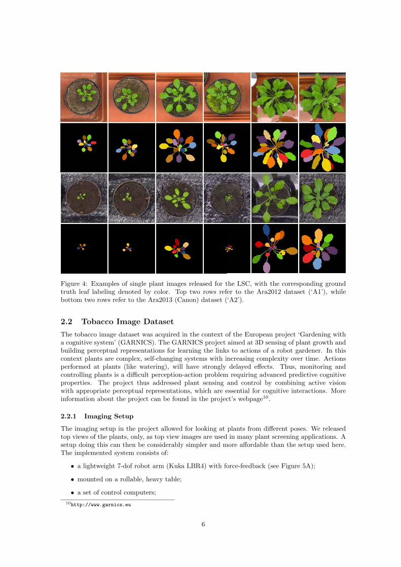
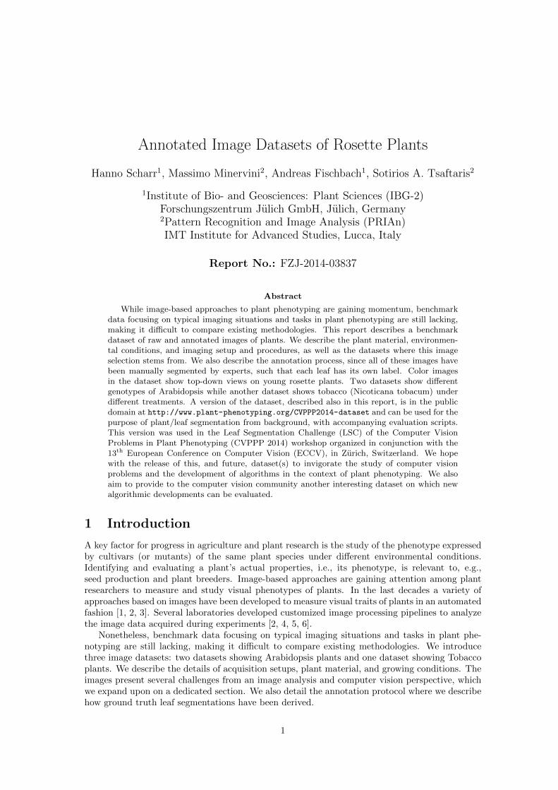
Figure 4: Examples of single plant images released for the LSC, with the corresponding groundtruth leaf labeling denoted by color. Top two rows refer to the Ara2012 dataset (‘A1’), whilebottom two rows refer to the Ara2013 (Canon) dataset (‘A2’).

2.2 Tobacco Image Dataset

The tobacco image dataset was acquired in the context of the European project ‘Gardening witha cognitive system’ (GARNICS). The GARNICS project aimed at 3D sensing of plant growth andbuilding perceptual representations for learning the links to actions of a robot gardener. In thiscontext plants are complex, self-changing systems with increasing complexity over time. Actionsperformed at plants (like watering), will have strongly delayed effects. Thus, monitoring andcontrolling plants is a difficult perception-action problem requiring advanced predictive cognitiveproperties. The project thus addressed plant sensing and control by combining active visionwith appropriate perceptual representations, which are essential for cognitive interactions. Moreinformation about the project can be found in the project’s webpage10.

2.2.1 Imaging Setup

The imaging setup in the project allowed for looking at plants from different poses. We releasedtop views of the plants, only, as top view images are used in many plant screening applications. Asetup doing this can then be considerably simpler and more affordable than the setup used here.The implemented system consists of:

• a lightweight 7-dof robot arm (Kuka LBR4) with force-feedback (see Figure 5A);

• mounted on a rollable, heavy table;

• a set of control computers;

10http://www.garnics.eu

6

Figure 5: Hardware setup of the robot gardener as used in the GARNICS project. (A) Therobot arm, in the lab environment. (B) Camera head with illumination and watering system. (C)Workspace with light, temperature, and humidity sensors.

• teaching buttons at the robots hand and on a switch panel;

• a head with cameras, light sources, and a watering system (see Figure 5B);

• digital and analog IOs for switching lights, pumps, or valves, hardware button presses, etc.;

• sensors for environment monitoring (see Figure 5C);

• a watering and nutrient solution dispensing system;

• high power white LED illumination allowing for photons fluxes of up to ∼2000 µmol s−1m−2

(see Figure 5A), switched off for imaging in an ‘inverse flashing’ fashion;

• low power white fluorescence illumination allowing for photons fluxes of up to ∼50 µmols−1m−2 (see Figure 5A), used for imaging.

The robot head consists of two stereo camera systems, black-and-white and color, each consist-ing of 2 Point-Grey Grashopper cameras with 5 megapixel (2448×2048, pixel size 3.45 µm) resolu-tion and high quality lenses (Schneider Kreuznach Xenoplan 1.4/17-0903). We added lightweightwhite and NIR LED light sources to the camera head.

7

Table 2: Summary of statistics of the acquired datasets where images for ‘A3’ were taken from.

Dataset Subjects Period Total Resolution Annotated Annotatedby start date images per plant plants images

23.01.2012 20 18 days 34560 5 megapixel 4 2616.02.2012 20 20 days 38400 5 megapixel 2 1315.05.2012 20 18 days 34560 5 megapixel 2 810.08.2012 20 30 days 57600 5 megapixel 5 36

Figure 6: Overview images of plants in final stages of 4 experiment runs. We refer to the experi-ments by their start date: A: 23.01.2012, B: 16.02.2012, C: 15.05.2012, D: 10.08.2012. Red squaresindicate the plants where images were taken for ‘A3’. Red 5 digit numbers are their plant IDsused to identify the plants (see Tables 3 and 4). Generally, plant IDs are increasing from left toright and top to bottom in the trays, respectively. IDs are A: 69665 – 69684, B: 69965 – 69984,C: 75984 – 76003, D: 79329 – 79348.

Using this setup, each plant was imaged separately from different but fixed poses. For each posein addition small baseline stereo image pairs were captured using each single camera, respectively,by a suitable robot movement, allowing for 3d reconstruction of the plant. For the top view pose,distance between camera center and top edge of pot varies between 15 cm and 20 cm for differentplants, but being fixed per plant, resulting in lateral resolutions between 20 and 25 pixel/mm.

Data released here stems from experiments aiming at acquiring training data for the robotgardener of the GARNICS project. Images were acquired every hour in a 24/7 manner for up to30 days. More details on the four experiments, from which the data is taken, can be found inTable 2. Overview images of the final stage of the plants from these experiments are shown inFigure 6.

8

Table 3: Time after experiment start per image in ‘A3’.

Training Testing

Image Plant Time Time Image Plant Time Time Image Plant Time TimeID [h] [d] ID [h] [d] ID [h] [d]

1 69665 6 0 28 69678 6 0 56 79329 132 62 78 3 29 78 3 57 204 93 174 7 30 174 7 58 276 124 222 9 31 222 9 59 349 155 270 11 32 270 11 60 444 196 428 18 33 343 14 61 516 227 69676 6 0 34 415 17 62 612 268 78 3 35 69684 6 0 63 709 309 174 7 36 78 3 64 79332 12 110 222 9 37 175 7 65 132 611 270 11 38 223 9 66 252 1012 294 12 39 271 11 67 372 1513 75984 9 0 40 343 14 68 492 2114 105 4 41 415 17 69 612 2615 178 7 42 69966 8 0 70 708 2916 289 12 43 80 3 71 79339 12 117 75985 9 0 44 148 6 72 133 618 81 3 45 200 8 73 252 1119 178 7 46 248 10 74 372 1620 275 11 47 296 12 75 492 2121 79348 12 0 48 344 14 76 613 2622 132 6 49 392 16 77 708 3023 253 11 50 69973 8 0 78 79347 13 124 373 16 51 94 4 79 132 625 493 21 52 147 6 80 253 1126 612 26 53 248 10 81 372 1627 709 30 54 344 14 82 493 21

55 79329 12 1 83 612 26

2.2.2 Plant and Leaf Annotations

As for the Arabidopsis datasets, annotations are provided in the form of images the same sizeof the originals, stored in PNG format [14]. A pixel with label index 0, depicted as black color,denotes background, while all other colors are used to uniquely identify the leaves of the plant inthe scene. Across the frames of the time-lapse sequence, label index and color do not depict thesame leaf.

For leaf segmentation we followed a similar procedure as described in Section 2.1.2, but using asimple color-based segmentation for foreground background segmentation. The result was manu-ally refined using a raster graphics editing software (Adobe Photoshop11). Next, within the binarymask of each plant, we delineated the individual leaves, following an approach completely basedon manual labeling. To reduce observer variability, the labeling procedure involved two users, oneannotating the dataset and inspecting the other. Figure 7 shows example plant images from thedataset, with corresponding annotations.

The type of annotations released together with the images reflect the intended use of thedatasets. The first level of information regards what pixels in an image belong, respectively,to a plant object or background. This serves as a ground truth to evaluate plant segmentationapproaches. Furthermore, the leaf labeling allows to use the datasets to test leaf segmentation orcounting approaches.

11http://www.photoshop.com/

9

Figure 7: Examples of single plant images ‘A3’ released for the LSC, with the correspondingground truth leaf labeling denoted by color.

2.2.3 Plant Material and Growing Conditions

Tobacco plants (Nicotiana tobacum cv. Samsun) were grown in 7 × 7 cm pots under constantlight conditions with a 16h/8h day/night rhythm. Light intensities were measured for each plantindividually (cf. Table 4).

Water was always provided by the robot system, where different but constant amounts perplant were given every two hours. Nutrients were either applied manually twice a week (12 mlHakaphos green 0.3%) or every other hour by the robot system (0.3 ml, 0.45 ml, or 0.9 ml Hakaphosgreen 1%). Treatments per plant are shown in Table 4. For water and nutrient solution dispensingthe GARNICS robot system positions small tubes, one for water and one for nutrient solution, atpredefined locations and pumps the liquids using an automated flexible-tube pump.

In the GARNICS project treatments were selected to produce training data for a cognitivesystem. The actual amounts of water and nutrient solution are therefore well adapted to the soilsubstrate such that the sets of plants show distinguishable performance of generally well growingplants. Finding an optimal treatment was left for the system. The soil used for the experiment(‘Kakteenerde’) has low nutrient content and dries relatively fast with an approximately exponen-tial behavior A = A0 exp(−t/τ), where τ ≈ 7 days.

Images show the growth stages from germination well into the leaf development stage, i.e. westarted our observations at growth stage 09 and typically stopped at stage 1009 to 1013 (accordingto the extended BBCH-scale presented in [16]), due to size restrictions. For each image of ‘A3’

10

Table 4: Plant treatments for tobacco plant experiments. Plants selected for ‘A3’ are highlighted.Treatments: T1 – T3: 0.6 ml, 1.8 ml, or 3.0 ml water every 2 hours, respectively, T4 – T5: 0.3 mlor 0.9 ml Hakaphos green 1% every 2 hours, T6: 0.9 ml water and 0.45 ml Hakaphos green 1%every 2 hours, T7 – T9: T1 – T3 plus 12 ml Hakaphos green 0.3% 2 times per week, respectively.

23.01.2012 16.02.2012 15.05.2012 10.08.2012Plant Treat- Light Plant Treat- Light Plant Treat- Light Plant Treat- Light

ID ment µmolm2s

ID ment µmolm2s

ID ment µmolm2s

ID ment µmolm2s

69665 T7 933 69965 T7 515 75984 T1 295 79329 T2 29569666 T8 1505 69966 T8 760 75985 T2 335 79330 T5 33569667 T9 1415 69967 T9 655 75986 T4 320 79331 T6 32069668 T7 1430 69968 T7 745 75987 T5 360 79332 T2 36069669 T8 1095 69969 T8 715 75988 T1 330 79333 T5 33069670 T9 1310 69970 T9 805 75989 T2 470 79334 T6 47069671 T7 2055 69971 T7 1200 75990 T4 570 79335 T2 57069672 T8 1825 69972 T8 1005 75991 T5 530 79336 T5 53069673 T9 1715 69973 T9 1060 75992 T1 600 79337 T6 60069674 T7 1365 69974 T7 990 75993 T2 545 79338 T2 54569675 T2 1200 69975 T2 790 75994 T4 545 79339 T5 54569676 T3 1910 69976 T3 1240 75995 T5 670 79340 T6 67069677 T1 1700 69977 T1 1035 75996 T1 630 79341 T2 63069678 T2 1455 69978 T2 1010 75997 T2 715 79342 T5 71569679 T3 1135 69979 T3 945 75998 T4 660 79343 T6 66069680 T1 705 69980 T1 560 75999 T5 470 79344 T2 47069681 T2 1110 69981 T2 880 76000 T1 590 79345 T5 59069682 T3 1030 69982 T3 755 76001 T2 550 79346 T6 55069683 T1 930 69983 T1 700 76002 T4 610 79347 T2 61069684 T2 700 69984 T2 620 76003 T5 565 79348 T5 565

acquisition times and plants shown are given in Table 3. Overview images of the final growthstages are given in Figure 6.

3 Analysis Challenges of the Acquired Image Data

Due to complexity of scene and plant objects, the datasets present a variety of challenges withrespect to analysis. Since our goal was to produce a good range of test images, several challengingsituations were allowed to occur by design.

For ‘A1’ and ‘A2’, occasionally, a layer of water in the tray due to irrigation causes reflections.As the plants grow, leaves tend to overlap, resulting in severe leaf occlusions. Nastic movementsmake leaves appear of different shape and size from one time instant to another. For ‘A3’ beneathshape changes due to nastic movements, also different leaf shapes appear due to different treat-ments. Under high illumination conditions plants stay more compact with partly wrinkled leaves,severely overlapping. Under lower light conditions leaves are more round and larger.

The Ara2012 dataset (‘A1’) presents a complex and changing background, that renders theplant segmentation task more challenging. A portion of the scene is slightly out of focus andappears blurred, and some images include external objects, such as tape or other fiducial markers.In some images, certain pots have moss on the soil, or have dry soil and appear yellowish (dueto increased ambient temperature for a few days). The Ara2013 dataset (‘A2’) presents a simplerscene (e.g., more uniform background, sharp focus, no moss), however it includes mutants withdifferent phenotypes related to rosette size (some genotypes produce very small seedlings) and leafappearance, with major differences in both shape and size. The GARNICS dataset (‘A3’) hasmuch higher image resolution, making computational complexity more relevant.

Also in the tobacco dataset plants undergo a wide range of treatments changing their appear-

11

ance dramatically, while Arabidopsis is known to have different leaf shape among mutants. Thus,shape-based segmentation is a challenging undertaking. In addition, self-occlusion, shadows, leafhairs, leaf color variations, and others make the scene even more complex.

4 The Leaf Segmentation Challenge Dataset Version

As we mentioned previously, a specially formatted part of these data was released to support theLeaf Segmentation Challenge component, of the Computer Vision Problems in Plant Phenotypingwhich was organized in conjunction with the European Conference of Computer Vision (ECCV),that was held in Zurich, Switzerland in September 2014.

As part of the benchmark data for the LSC we released three datasets, named respectively‘A1’, ‘A2’, and ‘A3’, consisting of single-subject images of arabidopsis and tobacco plants, eachaccompanied by manual annotation of plant and leaf pixels, examples of which are shown inFigures 4 and 7.

From the Ara2012 dataset, we extracted 161 images (width × height: 500×530 pixels), i.e.dataset ‘A1’, spanning a period of 12 days. Additional 40 images (width × height: 530×565pixels), i.e. ‘A2’ were extracted from the Ara2013 (Canon) dataset, and span a period of 26 days.From the tobacco dataset, we extracted 83 images (width × height: 2448×2048 pixels), i.e. ‘A3’.

The datasets were split into training and testing sets for the challenge. For the training subsetswere released in the public domain color images and annotations (i.e., 128, 31, and 27 images for‘A1’, ‘A2’, and ‘A3’, respectively). For the testing subsets, we released color images only (i.e., 33,9, and 56 for ‘A1’, ‘A2’, and ‘A3’, respectively) and kept the respective label images secret.

We should note that the LSC did not involve leaf tracking over time, therefore all plant imageswere considered separately, ignoring any temporal correspondence. Accordingly, the annotationswere released as indexed PNG images [14], where index 0 denotes background pixels and subsequentintegers denote leaf pixels. The images are mainly intended for plant and leaf segmentation, andrange from instances with well separated leaves and simple background, to more difficult exampleswith many leaf occlusions, complex leaf shapes, varying backgrounds, or plant objects not sharplyin focus.

File types and naming conventions. Plant images are encoded as PNG files and their size mayvary. Plants appear centered in the (cropped) image. Segmentation masks are image files encodedin PNG where each segmented leaf is identified with a unique (per image) integer value, startingfrom 1, where 0 is background. A color index palette is included within the file for visualizationreasons. The filenames have the form:

• plantXXX_rgb.png: the original RGB color image as true-color PNG file;

• plantXXX_label.png: the labeled image as indexed PNG file;

where XXX is an integer number. Note that plants are not numbered continuously.To evaluate submissions on the basis of testing data, we utilized several evaluation criteria in

a script, some of which are based on the Dice score of binary segmentations, measuring the degreeof overlap among binary segmentation masks:

Dice (%) =2 · TP

2 · TP + FP + FN(1)

where TP , FP , and FN represent the number of true positive, false positive, and false negativepixels, respectively, calculated by comparing algorithmic result and ground-truth segmentationmasks. Overall the criteria used where:

• SymmetricBestDice, the symmetric Average Dice among all objects (leaves), where for eachinput label the ground truth label yielding maximum Dice is used for averaging, to estimateaverage leaf segmentation accuracy;

12

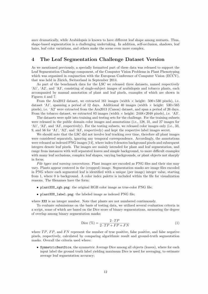
• FGBGDice, the Dice on the foreground mask (i.e., the whole plant assuming the union of alllabels different than background), to estimate how good the algorithm identifies plant frombackground;

• AbsDiffFGLabels, the absolute difference in object count, as number of leaves in groundtruth minus the algorithms results, to estimate how good the algorithm is in identifying thecorrect number of leaves present; and

• DiffFGLabels, the difference in object count, as number of leaves in ground truth minus thealgorithms results to estimate how good the algorithm is in identifying the correct numberof leaves present.

This dataset, and accompanying evaluation scripts, can be downloaded from: http://www.

plant-phenotyping.org/CVPPP2014-dataset.

5 Discussion and Conclusion

In this report we described design and implementation criteria adopted to collect three imagedatasets of growing Arabidopsis and Tobacco plants. This effort was intended to promote researchand development of computer vision approaches for plant phenotyping applications.

Parts of the datasets Ara2012 and Ara2013 have been already adopted to experimentallyvalidate new approaches that we presented in previous papers. In [13] we propose a distributedsensing and analysis framework for image-based plant phenotyping, and investigate application-aware image compression approaches. In [17] we propose color space transformations to improvecompression performance further. In [15] we propose a solution to analyze images from plantphenotyping experiments, with particular focus on plant segmentation. Finally, in [18] we exploreefficient approximations of complex image segmentation metrics, that could be adopted at thesensor.

The GARNICS project lead to 74 scientific and 23 non-specialist contributions, as well as 2patents. For more details we refer to the projects website12.

As a benefit to the scientific community, we are releasing in the public domain a speciallyformatted dataset, which contributed to the benchmark data for a leaf segmentation challenge.In the future, we do intend to use this technical report as a reference when releasing augmenteddatasets or datasets that could address different computer vision problems such as leaf tracking,leaf counting, leaf and plant detection, and others. We also do hope that this dataset and its futureversions, would be used from the computer vision community to learn suitable image statistics[19], adapt and test counting algorithms with [20] and without temporal information [21, 22,23], segmentation algorithms [24, 25, 26, 27, 28], multi-label segmentation [29, 30, 31, 32, 33] ordetection [34] approaches, and others. Additional depth information as can be computed fromstereo images [35] for the tobacco dataset, to be released in the future, may further facilitatesegmentation [36, 37, 38, 39].

6 Acknowledgements

The research work leading to the dataset ‘A3’ has received funding from the European Com-munity’s Seventh Framework Programme (FP7/2007-2013) under grant agreement no. 247947(GARNICS). Part of this work was performed within the German-Plant-Phenotyping Networkwhich is funded by the German Federal Ministry of Education and Research (project identifica-tion number: 031A053). The work leading to the arabidopsis datasets was also partially supportedby a Marie Curie Action: “Reintegration Grant” (grant #256534) of the EU’s Seventh FrameworkProgramme.

12http://www.garnics.eu

13

The authors would like to thank Prof. Pierdomenico Perata and his group from Scuola Su-periore Sant’Anna, Pisa, Italy, for providing us with plant samples and instructions on growthconditions of Arabidopsis. Finally, they also thank Fabiana Zollo and Ines Dedovic for assistancewith annotating part of the image data.

References

[1] Christine Granier, Luis Aguirrezabal, Karine Chenu, Sarah J. Cookson, Myriam Dauzat,Philippe Hamard, Jean-Jacques Thioux, Gaelle Rolland, Sandrine Bouchier-Combaud, AnneLebaudy, Bertrand Muller, Thierry Simonneau, and Francois Tardieu. PHENOPSIS, anautomated platform for reproducible phenotyping of plant responses to soil water deficit inarabidopsis thaliana permitted the identification of an accession with low sensitivity to soilwater deficit. New Phytologist, 169(3):623–635, January 2006.

[2] Achim Walter, Hanno Scharr, Frank Gilmer, Rainer Zierer, Kerstin A. Nagel, Michaela Ernst,Anika Wiese, Olivia Virnich, Maja M. Christ, Beate Uhlig, Sybille Junger, and Uli Schurr.Dynamics of seedling growth acclimation towards altered light conditions can be quantified viaGROWSCREEN: a setup and procedure designed for rapid optical phenotyping of differentplant species. New Phytologist, 174(2):447–455, 2007.

[3] M. Jansen, F. Gilmer, B. Biskup, K.A. Nagel, U. Rascher, A. Fischbach, S. Briem, G. Dreissen,S. Tittmann, S. Braun, I. De Jaeger, M. Metzlaff, U. Schurr, H. Scharr, and A. Walter.Simultaneous phenotyping of leaf growth and chlorophyll fluorescence via GROWSCREENFLUORO allows detection of stress tolerance in Arabidopsis thaliana and other rosette plants.Functional Pant Biology, Special Issue: Plant Phenomics, 36(10/11):902–914, 2009.

[4] Anja Hartmann, Tobias Czauderna, Roberto Hoffmann, Nils Stein, and Falk Schreiber. HT-Pheno: An image analysis pipeline for high-throughput plant phenotyping. BMC Bioinfor-matics, 12(1):148, 2011.

[5] Jonas De Vylder, Filip J. Vandenbussche, Yuming Hu, Wilfried Philips, and Dominique VanDer Straeten. Rosette Tracker: an open source image analysis tool for automatic quantifica-tion of genotype effects. Plant Physiology, 160(3):1149–1159, November 2012.

[6] Gerie van der Heijden, Yu Song, Graham Horgan, Gerrit Polder, Anja Dieleman, Marco Bink,Alain Palloix, Fred van Eeuwijk, and Chris Glasbey. SPICY: towards automated phenotypingof large pepper plants in the greenhouse. Functional Plant Biology, 39(11):870–877, 2012.

[7] Sotirios A. Tsaftaris and Christos Noutsos. Plant phenotyping with low cost digital camerasand image analytics. In Information Technologies in Environmental Engineering, Environ-mental Science and Engineering, pages 238–251. Springer Berlin Heidelberg, 2009.

[8] David Schneider. Camera hacking. IEEE Spectrum, 47(12):18–19, December 2010.

[9] Gonzalo Pajares and Jess Manuel de la Cruz. A wavelet-based image fusion tutorial. PatternRecognition, 37(9):1855–1872, 2004.

[10] Murali Subbarao and Gopal Surya. Depth from defocus: A spatial domain approach. Inter-national Journal of Computer Vision, 13(3):271–294, 1994.

[11] Roberto Ierusalimschy, Luiz Henrique de Figueiredo, and Waldemar Celes Filho. Lua – anextensible extension language. Software: Practice and Experience, 26(6):635–652, 1996.

[12] Japan Electronics and Information Technology Industries Association (JEITA). Exchangeableimage file format for digital still cameras: Exif version 2.2, April 2002.

14

[13] Massimo Minervini and Sotirios A. Tsaftaris. Application-aware image compression for lowcost and distributed plant phenotyping. In 18th International Conference on Digital SignalProcessing (DSP), pages 1–6, July 2013.

[14] W3C. Portable network graphics (PNG) specification, November 2003.

[15] Massimo Minervini, Mohammed M. Abdelsamea, and Sotirios A. Tsaftaris. Image-based plantphenotyping with incremental learning and active contours. Ecological Informatics, 2013.

[16] CORESTA. A scale for coding growth stages in tobacco crops, February 2009.

[17] Massimo Minervini, Cristian Rusu, and Sotirios A. Tsaftaris. Unsupervised and supervisedapproaches to color space transformation for image coding. In 21st International Conferenceon Image Processing (ICIP), October 2014.

[18] Massimo Minervini, Cristian Rusu, and Sotirios A. Tsaftaris. Learning computationally effi-cient approximations of complex image segmentation metrics. In 8th International Symposiumon Image and Signal Processing and Analysis (ISPA), pages 60–65, September 2013.

[19] M. Heiler and C. Schnorr. Natural image statistics for natural image segmentation. Interna-tional Journal of Computer Vision, 63:5–19, 2005.

[20] L. Fiaschi, K. Gregor, B. Afonso, M. Zlatic, and F. A. Hamprecht. Keeping count: Leverag-ing temporal context to count heavily overlapping objects. In International Symposium onBiomedical Imaging (ISBI), pages 656–659, 2013.

[21] C. Arteta, V. Lempitsky, J. A. Noble, and A. Zisserman. Learning to detect partially overlap-ping instances. In IEEE Conference on Computer Vision and Pattern Recognition (CVPR),2013.

[22] Victor S. Lempitsky and Andrew Zisserman. Learning to count objects in images. In Advancesin Neural Information Processing Systems (NIPS), pages 1324–1332, 2010.

[23] Luca Fiaschi, Ullrich Kothe, Rahul Nair, and Fred A. Hamprecht. Learning to count withregression forest and structured labels. In International Conference on Pattern Recognition(ICPR), pages 2685–2688, 2012.

[24] T.F. Chan and L.A. Vese. Active contours without edges. IEEE Transactions on ImageProcessing, 10(2):266–277, February 2001.

[25] L.A. Vese and T.F. Chan. A multiphase level set framework for image segmentation usingthe Mumford and Shah model. International Journal of Computer Vision, 50(3):271–293,December 2002.

[26] M. Rousson and R. Deriche. A variational framework for active and adaptative segmentationof vector valued images. In Proceedings of the Workshop on Motion and Video Computing,MOTION ’02, pages 56–61, Washington, DC, USA, 2002. IEEE Computer Society.

[27] R. Fahmi and A.A. Farag. A fast level set algorithm for shape-based segmentation withmultiple selective priors. In IEEE International Conference on Image Processing (ICIP),pages 1073–1076, 2008.

[28] Leah Bar, Tony F. Chan, Ginmo Chung, Miyoun Jung, Nahum Kiryati, Rami Mohieddine,Nir Sochen, and Luminita A. Vese. Mumford and Shah model and its applications to imagesegmentation and image restoration. In Otmar Scherzer, editor, Handbook of MathematicalMethods in Imaging, pages 1095–1157. Springer New York, 2011.

[29] Minsu Cho, Young Min Shin, and Kyoung-Mu Lee. Unsupervised detection and segmenta-tion of identical objects. In IEEE Conference on Computer Vision and Pattern Recognition(CVPR), pages 1617–1624, June 2010.

15

[30] C. Nieuwenhuis, E. Toeppe, and D. Cremers. A survey and comparison of discrete andcontinuous multi-label optimization approaches for the Potts model. International Journalof Computer Vision, 104(3):223–240, September 2013.

[31] C. Nieuwenhuis and D. Cremers. Spatially varying color distributions for interactive multilabelsegmentation. IEEE Transactions on Pattern Analysis and Machine Intelligence, 35(5):1234–1247, May 2013.

[32] Xuming He and S. Gould. Multi-instance object segmentation with exemplars. In IEEEInternational Conference on Computer Vision Workshops (ICCVW), pages 1–4, December2013.

[33] Xuming He and S. Gould. An exemplar-based CRF for multi-instance object segmentation.In IEEE Conference on Computer Vision and Pattern Recognition (CVPR), 2014.

[34] Olga Barinova, Victor S. Lempitsky, and Pushmeet Kohli. On detection of multiple objectinstances using hough transforms. IEEE Transactions on Pattern Analysis and MachineIntelligence, 34(9):1773–1784, 2012.

[35] B. Biskup, H. Scharr, U. Schurr, and U. Rascher. A stereo imaging system for measuringstructural parameters of plant canopies. Plant, Cell and Environment, 30:1299–1308, 2007.

[36] B. Dellen, G. Alenya, S. Foix, and C. Torras. Segmenting color images into surface patchesby exploiting sparse depth data. In WACV, 2011.

[37] G. Alenya, B. Dellen, and C. Torras. 3D modelling of leaves from color and tof data forrobotized plant measuring. In IEEE International Conference on Robotics and Automation,pages 3408–3414, 2011.

[38] M. Wallenberg, M. Felsberg, and P.-E. Forssen. Leaf segmentation using the Kinect. InProceedings SSBA’11 Symposium on Image Analysis, Mar 2011.

[39] M. Wallenberg, M. Felsberg, P.-E. Forssen, and B. Dellen. Channel coding for joint colourand depth segmentation. In Proceedings of Pattern Recognition 33rd DAGM Symposium,Frankfurt/Main, Germany, August 31 - September 2, volume LNCS 6835, pages 306–315,2011.

16