annex a: impacts of comprehensive climate and energy policy options on the u.s. economy

Impacts of Comprehensive Climate and Energy Policy Options on the U.S. Economy 73

The methodologies summarized in this Annex are used to extrapolate the quantification results (greenhouse gas [GHG] reduction potentials and per-ton cost/savings, i.e., cost-effectiveness) for the 23 “super options” analyzed by the Center for Climate Strategies (CCS) in 16 states. The 23 policies and measures in the 16 states’ action plans are extrapolated to the rest of the states. The 16 states with CCS-analyzed action plans include: Alaska, Arkansas, Arizona, Colorado, Florida, Iowa, Maryland, Michigan, Minnesota, Montana, New Mexico, North Carolina, Pennsylvania, South Carolina, Vermont, and Washington (“existing states”). The methodology was applied to each of the remaining 34 U.S. states (“new states”) to derive both the reduction potentials and cost-effectiveness of each individual super option.

I. Summary

In Section II of this Annex, three methods were evaluated to extrapolate the quantification results of the Energy Supply (ES), Residential Commercial, and Industrial (RCI), and Agriculture, Forestry, and Waste Management (AFW) super options in the 16 existing states where CCS had done analysis for climate action plans to the remaining non-Southern Governors’ Association (SGA) states. These methods are known as Analogous State, Simple-Average, and Weighted-Average. Of the three, the Weighted-Average Method was selected because of its superior performance. For every new state, this method utilizes the data from all of the 16 existing states in the extrapolation calculation for each super option. By applying this approach, rather than using a simple average, higher weights are assigned to existing states that share similarities with the new state. Also, this approach captures most of the major strengths of the Analogous State Method, but does not place the onus of comparison on any single state. It may still place too much emphasis on existing states that are different from the new state, but this is moderated somewhat in that different weights are used for each set of options.

The Weighted-Average Method develops a mathematical approach to quantify the similarities among individual states. The similarity measurement is established based on how each state ranks relative to others in terms of key factors affecting the reduction potentials and cost/savings of various mitigation/sequestration policy options. Theoretically, among the three alternative methods, the Weighted-Average Method can best capture the underlying factors that explain the variances in the quantification results of the super options among the 16 existing states.

In Section III, the VISION model is described, which was used to analyze the GHG reduction potentials and cost/savings associated with the implementation of the super options from the Transportation and Land Use (TLU) sector. The VISION model is a peer-reviewed spreadsheet scenario modeling tool that was developed by the United States Department of Energy (USDOE) (Ward, 2008). The VISION model is updated on an annual basis. The most recent version of the Voluntary Innovative Sector Initiatives (VISION) model was used for the analysis of the TLU sector.

In Section IV, two versions of national cost curves (full stakeholder implementation version and congressional target implementation version) are developed based on the extrapolation analysis of the GHG reduction potentials and cost-effectiveness of super options from the existing states to the remaining states in the U.S.

annex a

» Estimation Methodology for GHG Reduction Potentialand Cost-Effectiveness of Super Options

74 Johns Hopkins University and Center for Climate Strategies

II. Extrapolation Methodology for the ES, RCI, and AFW Super Options

Definitions and Descriptions of the Methods Used

A. Analogous State Method

In this method, we identify the analogous state from the 16 existing states to be used as the extrapolation basis for each of the new states in the cost curve extrapolation. An analogous state is not necessarily a neighboring state of the new state. It is more important that the analogous state and the new state share similar characteristics that are key factors affecting the GHG reduction potentials and costs/savings associated with the reduction. For each new state/territory, the analogous state is identified for each of the three sectors (Energy Supply [ES]. Residential, Commercial, and Industrial [RCI], and Agriculture, Forestry, and Waste Management [AFW]), since the key factors affecting the reductions and cost/savings are quite different in various sectors. Appendix A lists sectoral key factors. Appendix B gives an example of how the analogous state for the Demand Side Management Programs option for an example new state is determined.

After the analogous state is selected (see the details in Appendix B), the extrapolation to the new states is performed through the following steps:

1. For the ES options, the ratio of total emissions from the Power sector between the new state and the analogous state is computed.1 For the RCI options, the ratio of emissions from the Commercial and Industrial sectors between the new state and the analogous state is computed for the Combined Heat and Power option. Emissions from the Residential, Commercial, and Industrial sectors are computed for the other RCI options.2 For the AFW options, the ratio of applicability between the new and analogous states is computed (for example, the variable used to determine the applicability of the Livestock Manure option is the estimated total state population of dairy cattle, beef cattle, and swine. The variable used to determine the applicability of the Reforestation/Afforestation option is the total acres of combination of agricultural land and other non-forest, non-urban land).

2. The new state over the analogous state ratio of total sectoral emissions or the ratio of applicability is multiplied by the emission reduction potentials of the super option in the analogous state to get the estimate of the GHG reduction potentials in the new state. (For example, if the ratio of the estimated total population of dairy cattle, beef cattle, and swine in the new state and the analogous state is 2:1, the estimated GHG reduction potentials of the Livestock Manure option in the new state are two times that in the analogous state.)

3. The cost-effectiveness (i.e., per-ton cost/saving of GHG removed) of each super option in the new state is assumed to be same as in the analogous state.

B. Simple-Average Method

In this method, instead of using data from one analogous state to do the extrapolation, for each option, data from all the 16 existing states are utilized in the extrapolation analysis for the new states. In contrast to the Weighted-Average Method to be described below, this method treats the data from the 16 existing states equally in the extrapolation calculation for the new state.

1. For the super options of Carbon Capture and Sequestration and Coal Plant Efficiency Improvements, geological CO2 storage resource and total electricity generation from coal are used , respectively (instead of total emissions from the Power sector) in this extrapolation step.2. For High Performance Buildings, Appliance Standards, and Building Codes options, 100% of the emissions from the Residential and Commercial sectors is included. For the Industrial sector, only 9.4% of the sectoral emissions is included. This is because, according to the EIA 2002 Energy Consumption by Manufacturers report, approximately 9.4% of the industrial energy use in the U.S. is for heating, ventilating and air conditioning (HVAC), lighting, and other facility support (see http://www.eia.doe.gov/emeu/mecs/mecs2002/data02/shelltables.html). For the Demand Side Management option, total emissions from the Industrial sector are included, since this option would cover reductions in emissions from various industrial processes.


The extrapolation steps are:

1. For the ES and RCI super options, the ratio of emissions from the relevant sector between the new state and each of the 16 existing states is computed, while for the AFW options, the ratio of applicability between the new and each of the 16 existing states is computed.

2. The new state over the existing state ratio of total sectoral emissions or the ratio of applicability is multiplied by the emission reduction potentials of the super option in the existing state to get the estimate of the GHG reduction potentials in the new state. This calculation is made 16 times, each time using the numbers from one existing state as the extrapolation basis.

3. The simple average of the 16 estimates of GHG reduction potentials computed in step 2 is calculated as the final estimate for the new state.

4. The simple average of the cost-effectiveness of the 16 states is computed as the estimate for the new state.

5. Please note for options that are not recommended in all the 16 states, simple average is calculated by averaging the numbers from those states that included the options in their state climate action plan recommendations.

C. Weighted-Average Method

Similar to the Simple-Average Method, data from all 16 existing states are utilized in the extrapolation computation for any given new state. The difference is that weights for the 16 existing states are computed based on several key sectoral factors and state characteristics, so that existing states that share similarities with the new state will be given a higher weight in the extrapolation analysis. Appendix B contains an example of how the weights for the Demand Side Management Program option are computed for an example new state.

After the calculation of the weights for the 16 existing states (see Appendix B for details), the extrapolation steps are:

1. For the ES and RCI super options, the ratio of emissions from the relevant sector between the new state and each of the 16 existing states is computed, while for the AFW options, the ratio of applicability between the new and each of the 16 existing states is computed.

2. The new state over the existing state ratio of sectoral emissions or the ratio of applicability is multiplied by the emission reduction potentials of the super option in the existing state to get the estimate of the GHG reduction potentials in the new state. This calculation is made 16 times, each time using the numbers from one existing state as the extrapolation basis.

3. The weighted average of the 16 estimates of GHG reduction potentials computed in step 2 is calculated as the final estimate for the new state.

4. The weighted average of the cost-effectiveness of the 16 states is computed as the estimate for the new state.

5. Again, for options that are not recommended in all the 16 states, weighted average is calculated by averaging just the numbers from those states that included the options in their state climate action plan recommendations.

Sample Calculations for the Three Alternative Approaches

In this section, we use the RCI super option Demand Side Management Programs as an example to illustrate how the three alternative extrapolation methods work. Table A-1 lists the options from the 16 existing states on Demand Side Management Programs.


Table A-1. List of the Updated State Options on Demand Side Management Programs

Option Option Description2020 GHG

Reductions (MMtCO2e)

Cost–Effectiveness ($/tCO2e)

AK: ESD-2/4/6 Energy Efficiency for Residential, Commercial, and Industrial Customers, 2% per year 1.07 –$74.01

AR: RCI-2b Utility and Non-Utility Demand Side Management (DSM) and Energy Efficiency for Electricity 2.39 –$5.70

AZ: Combination of RCI-1 and RCI-8*

RCI-1: Efficiency Goals, Funds, Incentives, and Programs

RCI-8: Electricity Pricing Strategies

9.58 –$42.49

CO: Combination of RCI-1, RCI-7, and RCI-5b*

RCI-1: Expand DSM Programs of All Electric and Gas Utilities

RCI-5b: Inverted Block Rates to Fund Energy Efficiency (Less Stringent targets)

RCI-7: Electricity Smart Metering with Time-of-Use Rates and In-Home or In-Office Displays for All Residential, Commercial, and Industrial Consumers

8.40 –$62.78

FL: ESD-12 DSM/Energy Efficiency Programs, Funds, or Goals for Electricity 17.24 –$51.32

IA: Combination of EEC-2, EEC-5, EEC-12*

EEC-2: Demand Side Management/Energy Efficiency Programs for Natural Gas

EEC-5: Incentive Mechanisms for Achieving Energy Efficiency

EEC-12: Demand Side Management/Energy Efficiency Programs for Electricity

5.17 –$26.74

MD: RCI-2 Demand Side Management for Electricity and Natural Gas 4.48 –$63.70

MI: RCI-2

RCI-2: Existing Building Energy Efficiency Incentives, Assistance, Certification and Financing (MI RCI-2 is split 53% and 47% between DSM option and High Performance Buildings option)

15.29 –$30.27

MN: RCI-1 RCI-1 Maximize Savings from the Utility Conservation Improvement Program (CIP) 9.51 –$72.96

MT: Combination of RCII-1, RCII-2, RCII-10, RCII-11, and RCII-13*

RCII-1: Expand Energy Efficiency (EE) Funds

RCII-2: Market Transformation and Technology Development Programs

RCII-10: Industrial Energy Audits and Recommended Measure Implementation

RCII-11: Low-Income Energy Efficiency Programs

RCII-13: Metering Technologies with Opportunity for Load Management and Choice

2.43 –$21.03

NC: Combination of RCI-1, RCI-2, and RCI-11*

RCI-1: Demand Side Management Programs for the RCI Sectors—Recommended Case: “Top-Ten States” EE Investment

RCI-2: Expand Energy Efficiency Funds

RCI-11: Residential, Commercial, and Industrial Energy and Emissions Technical Assistance and Recommended Measure Implementation

17.86 –$43.99


Option Option Description2020 GHG

Reductions (MMtCO2e)

Cost–Effectiveness ($/tCO2e)

NM: Combination of RCI-1, RCI-2, RCI-3, RCI-6, and RCI-9*

RCI-1: Electricity DSM (over/above BAU)

RCI-2: Natural Gas DSM (over/above BAU)

RCI-3: Regional Market Transformation Alliance

RCI-6: Rate Design

RCI-9: Government Agency Requirements and Goals (Including Procurement)—Focus on Operations

1.69 –$37.98

PA: Combination of RCI-10, RCI-11, Ind-2, and Elec-3*

RCI-10: Demand Side Management—NG

RCI-11: Demand Side Management—Electricity

Ind-2: Industrial DSM

Elec-3: Stabilize Load Growth

20.90 –$13.99

SC: Combination of RCI-1 and RCI-2*

RCI-1: Demand Side Management (DSM)/Energy Efficiency Programs, Funds, or Goals for Electricity

RCI-2: Demand Side Management (DSM)/ Energy Efficiency Programs, Funds, or Goals for Natural Gas, Propane, and Fuel Oil

7.35 –$41.08

VT: ESD-1 ESD-1: Evaluation and Continuation / Expansion of Existing DSM for Electricity and Natural Gas 0.98 –$44.65

WA: Combination of RCI-1 and RCI-5*

RCI-1: Demand Side Management Programs Energy Efficiency Programs, Funds, or Goals for Natural Gas, Propane, and Fuel Oil

RCI-5: Rate Structures and Technologies to Promote Reduced GHG Emissions

1.57 –$50.80

* The overlaps between these options are adjusted before combining them in the table. The cost-effectiveness is the weighted average of these options (using GHG emission reductions as weights). AK = Alaska; AZ = Arizona; CO = Colorado; IA = Iowa; MI = Michigan; MN = Minnesota; MT = Montana; NM = New Mexico; PA = Pennsylvania; VT = Vermont; WA = Washington; DSM = demand side management; BAU = Business As Usual; EE = energy efficiency; NG = natural gas; ESD = Energy Supply and Demand; RCI =Residential, Commercial, and Industrial; RCIII = Residential, Commercial, Institutional,and Industrial; GHG = greenhouse gas; MMtCO2e = million metric tons of carbon dioxide equivalent; $/tCO2e = dollars per metric ton of carbon dioxide equivalent (reduced).

Table A-2 presents an example of the extrapolation results of the Demand Side Management Programs option to a hypothetical new state using the three alternative approaches. In the calculation, we assume:

1. For the new state, the weights computed for the 16 existing states (please see the method elaborated in Appendix B at the end of this Annex) are:

New State Weights Computed for Existing States

Alaska 4%

Arkansas 13%

Arizona 5%

Colorado 4%

Florida 4%

Iowa 6%

Maryland 3%

Table A-1, continued from previous page


New State Weights Computed for Existing States

Michigan 5%

Minnesota 4%

Montana 6%

North Carolina 6%

New Mexico 7%

Pennsylvania 6%

South Carolina 19%

Vermont 3%

Washington 5%

2. The ratios of the total emissions from the RCI sector between the new state and the 16 existing states are:

New State Ratio of Total Emissions from the RCI Sector

Alaska 3:1

Arkansas 2:1

Arizona 1.7:1

Colorado 1.3:1

Florida 1:2

Iowa 1.4:1

Maryland 1.3:1

Michigan 1.6:1

Minnesota 1.2:1

Montana 5.5:1

North Carolina 1:1.3

New Mexico 2.2:1

Pennsylvania 1:1.8

South Carolina 1.5:1

Vermont 14:1

Washington 2.5:1

Some states had slight variants on the sector names. For example, Alaska, Florida, and Vermont developed Energy Supply and Demand (ESD) policies. While most states used RCI, Iowa termed this sector Energy Efficiency and Conservation (EEC).

Table A-2. Illustrative Extrapolation Analysis Results of the Demand Side Management Programs Option Using the Three Alternative Approaches

Method 2020 GHG Reductions (MMtCO2e)

Cost-Effectiveness ($/tCO2e) Notes

Analogous State Method 11.03 –$41.08 In the Analogous State Method, South Carolina is identified as the analogous state to the new state.

Simple-Average Method 10.23 –$42.72

Weighted-Average Method 9.92 –$37.42

GHG = greenhouse gas; MMtCO2e = million metric tons of carbon dioxide equivalent; $/tCO2e = dollars per metric ton of carbon dioxide equivalent (reduced emissions).


Comparison of the Three Alternative Approaches

A. Analogous State Method

Pros:

»» Easy to understand.

»» Less time-consuming than the Weighted-Average Method.

»» Utilizes the sectoral key factors in the selection of the analogous state.

Cons:

»» May not seem to adequately consider political issues.

»» For each option, only data from one existing state are utilized in the extrapolation. If this state is not adequately representative of the new state, then the results will be biased.

B. Simple-Average Method

Pros:

»» Easy to understand.

»» Least time-consuming method among the three.

»» For each option, data from all the 16 existing states are utilized in the calculation.

Cons:

»» Sectoral key factors are not used in this method.

»» For each option, all the new states will have the same cost-effectiveness, which would be the average of those of the 16 existing states.

C. Weighted-Average Method

Pros:

»» For each option, data from all the 16 existing states are utilized in the calculation.

»» This method utilizes the sectoral key factors in the weightings computation, which potentially can capture some of the similarities and differences across the states.

Cons

»» Most time-consuming method.

We also need to acknowledge that additional variation exists that cannot be readily captured by any of the methods. This variation is a natural outcome of the stakeholder-driven processes that allow for local knowledge, as well as variation in the policy design and goals among states. An example of this in the RCI sector would be that, in some existing states, energy-efficient measures in new construction might be combined in the Demand Side Management super option, while in other states these measures might fall into the High Performance Buildings super option. However, this becomes a non-issue when looking at total RCI emission reduction potentials (all RCI super options together) among new and existing states.

In sum, the Weighted-Average Method was selected from the three alternative extrapolation approaches to use in this study. The Weighted-Average Method develops a mathematical approach to quantify the similarities among individual states. The similarity measurement is established based on how each state ranks relative to others in terms of key factors affecting the reduction potentials and cost/savings of various mitigation/sequestration policy options. Theoretically, among the three alternative methods, the Weighted-Average Method can best capture the underlying factors that explain the variances in the quantification results of the super options among the 16 analyzed states. The only drawback of the Weighted-Average Method is that, even with weighting, it may still place too much emphasis on existing states that are different from the new state. This is moderated somewhat in that different weights are used for each set of options from different sectors.


III. Extrapolation Methodology for the TLU Super Options, Including Description of the USDOE VISION Model

Analysis of the Scenario to Transition to Lower-Carbon Methods of Moving Goods (Covering Anti-Idling and Freight Mode Shift)

To quantify the GHG emission reductions and cost-effectiveness of a transition to low-carbon methods of moving goods, three policies were examined:

1. Encouraging truck stop electrification (TSE);

2. Promoting the use of plug-in trailer refrigeration units (TRUs); and

3. Encouraging increased use of shuttle rail to move goods.

The effects of encouraging TSE were calculated by estimating the number of expected TSE units during the policy analysis period (i.e., 2009 to 2020), the GHG reductions attributed to a TSE unit relative to traditional engine idling, and the cost of expanding TSE units on a per-unit basis. The 2009 count of TSE units was estimated using information from USDOE.3 The number of truck stops is assumed to increase at the same growth rate as TSE units in New York. The compound annual growth rate for TSE units in New York was estimated in a recently completed New York State Energy Research and Development Authority (NYSERDA) study. GHG emissions relative to traditional idling practices and TSE unit costs were gleamed from a 2004 Transportation Research Board (TRB) study.4

The number of TRUs was estimated by scaling the number of TRUs in New York, according to the same recently completed NYSERDA study, by the population ratio of the two states. Plugged-in TRU GHG emissions relative to traditional idling practices and TRU unit costs were gleaned from a 2004 TRB study.5 The analysis utilizes a perpetual inventory of TRUs that enter and exit the TRU population as old units are phased out and new units are purchased over time.

The effects of encouraging increased use of freight rail diversion were estimated from a national-level estimate of the impacts of freight rail diversion. The share of the estimated GHG reduction and cost estimates were scaled using the current share of national rail freight movement, which is estimated to be 1.3% of all national rail-transported freight and available rail lines.

Annual percentage reductions in carbon dioxide-equivalent (CO2e) emissions are applied to a baseline forecast of GHG emissions for New Jersey to determine the reduction in CO2e emissions. Omitted gasoline and ethanol sales are multiplied by a scaling factor and forecasted U.S. fuel prices. TRU and TSE program costs are calculated by multiplying the cost of a TRU or TSE unit by the number of TRUs and TSEs expected to be sold over time minus the fuel savings expected from introducing the new technology. The number of TSEs sold is based on a growth rate assigned to the number of TSEs. The number of TRUs is scaled down from the number of TRUs in New York based on the population ratio of the two states.

Rail freight diversion is estimated by scaling down the national-level costs of rail freight diversion based on the current share of rail freight that is transported through a state according to Freight Analysis Framework estimates. To calculate the costs and levels of rail diversion that might be realized, a credible source is the American Association of State Highway and Transportation Officials’ (AASHTO’s) Freight-Rail Bottom Line Report.6 The report addresses concerns about the capacity of the nation’s freight transportation system, especially the freight-rail system, to keep pace with the expected growth of the economy over the next 20 years. The report finds that relatively small public investments in the nation’s freight railroads can be leveraged into relatively large public benefits for the nation’s highway infrastructure, highway users, and freight shippers.

3. U.S. Department of Energy, http://www.afdc.energy.gov/afdc/locator/tse/state.4. Transportation Research Board. 2004. “Long-Haul Tractor Idling Alternative.” Table 1. See http://epa.gov/smartway/documents/dewitt-study.pdf.5. Ibid.6. American Association of State Highway and Transportation Officials. Transportation Invest in America Freight-Rail Bottom Line Report. Available at: http://freight.transportation.org/doc/FreightRailReport.pdf.

http://www.afdc.energy.gov/afdc/locator/tse/state

http://freight.transportation.org/doc/FreightRailReport.pdf


Analysis of Scenarios Describing Vehicle Efficiency Incentives and Greater Use of Biofuels

For these two scenarios, the VISION model was utilized as the central analytical tool to measure the emissions and costs impacts of both a higher-biofuels-usage scenario and a scenario in which effective incentives resulted in a more fuel-efficient light duty fleet.

The VISION model was developed by USDOE to provide estimates of the potential energy use, oil use, and carbon emission impacts of advanced light and heavy duty highway vehicle technologies and alternative fuels from the present through the year 2100.7 The VISION model uses vehicle survival and age-dependent use characteristics to project total light and heavy vehicle stock, total vehicle miles traveled (VMT), and total energy use by technology and fuel type by year, given market penetration and vehicle fuel economy assumptions developed exogenously. Total carbon emissions for on-highway vehicles by year are also estimated because life-cycle carbon coefficients for various fuels are included in VISION. These coefficients are consistent with the Greenhouse Gases, Regulated Emissions, and Energy Use in Transportation (GREET) model, which was also developed by USDOE.

The VISION model considers a set of input parameters. Default parameter values taken from USDOE’s Annual Energy Outlook (AEO) reference case are in place. The default parameter values are regularly updated, usually on an annual basis, to reflect the most recent AEO reference case, which was 2009 for this analysis. All input values can be changed by the user to customize the simulation. Input parameters include:

»» Car market penetration and fuel economy ratio;

»» Light truck market penetration and fuel economy ratio;

»» Light truck share of total light duty vehicle market;

»» Fuel type (including hydrogen and ethanol via multiple production pathways) and price;

»» VMT, including growth rate and elasticity to the cost of driving;

»» Heavy vehicle fuel economy, market share, and alternative fuel use; and

»» Light vehicle cost.

The model generates output values, by vehicle type (car, light truck, and heavy truck). The output totals include (Ward, 2008):

»» Energy use by fuel type (oil, compressed natural gas, Fischer-Tropsch diesel, biodiesel, methanol, hydrogen, electricity, ethanol, and other fuels);

»» Full-fuel-cycle carbon emissions (million metric tons [MMt] of CO2e);

»» Full-fuel-cycle GHG emissions (MMtCO2e);

»» Fuel expenditures (billion 2005$);

»» Fuel expenditures as a percentage of gross domestic product; and

»» Light vehicle miles per gallon gasoline equivalent (energy).

VISION is a well-documented, well-used, and well-published model. A 2006 American Association of State Highway and Transportation Officials and Transportation Research Board study recommended the use of the VISION tool for state-level and multi-state analyses. The VISION model is the most widely used tool for state-level analyses of transportation energy and climate emissions scenarios. In addition to the SGA region, the states where VISION has been used include California, New Mexico, Colorado, New York, and New Jersey. The northeastern states are developing a regionally tailored version of the VISION tool.

7. VISION is a public access tool that may be found at : http://www.transportation.anl.gov/modeling_simulation/VISION/index.html.


VISION can be tailored to specific states or multi-state regions when locally specific data are available to replace any default data.

VISION is an open-source, fully transparent tool, so many researchers have used and adapted it to their own needs, replacing some market assumptions (e.g., vehicle demand growth, alternative-fueled vehicle cost) with their own assumptions for different analyses. USDOE’s Argonne National Laboratory continues to maintain and update the model, and the key developers are readily available to answer questions. VISION is not a behavioral model. Rather, it is a complex accounting system that allows users to modify assumptions as needed. It provides a perpetual inventory of the vehicle fleet through 2100 by type, size, efficiency, technology, and use.

In order to generate estimates of the costs and impacts of a biofuels scenario, projected national trends of increased biofuels consumption by light duty and heavy duty vehicles were magnified from a baseline projection to a projection of 20% consumption by volume in 2020. (The baseline projection is roughly half the scenario projection.) In addition, market penetration of vehicles capable of using biofuels in the light duty market was also manipulated in line with fuel consumption trend adjustments. Those inputs were then utilized in the VISION model to estimate scenario costs for vehicles and fuels, as well as estimates for emissions from the light duty and heavy duty vehicle fleets.

In order to generate estimates of the costs and GHG reduction potentials of a vehicle purchase incentives scenario, estimates of the impacts of such a program were drawn from Greene et al.’s 2005 research on vehicle efficiency purchase incentives. The Greene study’s estimates of efficiency impacts were used as inputs in VISION to estimate scenario costs for vehicles and fuels, as well as estimates for emissions from the light duty vehicle fleet.

Analysis of Scenarios Describing Application of Smart Growth Principles and Greater Reliance on Public Transit

The VISION model was also used for the travel activity analyses. Since the amount and types of travel activity are important factors in the determination of fuel use, the VISION model was used as a complement to option-specific spreadsheet analyses for TLU-5: Smart Growth/ Land Use and for TLU-6: Transit. The complementary use of VISION with the VMT-related options included three specific uses that are particularly noteworthy:

»» Use of VISION to contribute to energy and GHG outputs under baseline forecast conditions,

»» Use of life-cycle GHG emissions factors to convert reductions in VMT to reductions in GHG potential, and

»» Use of VISION to run alternative scenarios with higher (baseline) VMT and lower (with TLU-5 and TLU-6) VMT reduction, so as to account for overlap between the VMT-related measures and other measures.

The option-specific spreadsheet analyses and parameters for analyses of smart growth and transit were taken from the spreadsheets and policy designs developed for the CCS states with completed state plans. The option-specific spreadsheets and parameters for smart growth incorporate the state-specific factors in terms of the baseline conditions for auto use and public transportation use, and in terms of their baseline VMT that may be associated with land development patterns.

The spreadsheet scenarios take into account the specific economic and transportation characteristics of each state, while extrapolating from the CCS state results on the basis of the policy descriptions and policy designs that reflect the stakeholder consensus and recommendations in the state plans. In this way, the national results represent an extrapolation of the results from the CCS state plans, adjusted for the key factors described and state-specific characteristics.


The analyses of the Transportation sector took into account key factors and state characteristics that included:

A. Population growth and density,

B. Energy consumption by the Transportation sector,

C. Shares of urban, suburban, and rural population,

D. Forecasted VMT levels and growth,

E. Shares of use of public transportation, and

F. Current and projected fleet mixes for passenger, heavy duty, and freight vehicles.

The discussion below shows step-by-step descriptions where the above key factors and state characteristics are factored in by showing the letters (A through F) following the step where these factors were taken into account. In addition to the factors applied, the initial judgments on the feasibility of VMT goals as determined by stakeholders in the CCS states with completed plans took into account many local and state-specific factors that are reflected in the goal levels.

Following is a step-by-step description of the smart growth and transit options spreadsheet analysis:

»» Use VISION 2008 (most recent VISION available), results with updated AEO 2009 fuel forecast for baseline VMT forecast consistent with adopted federal Corporate Average Fuel Economy standards. (Factor B)

»» Factor in state-specific motor vehicle registrations and state-specific motor vehicle use for the states. (Factor F)

»» Estimate the baseline state-specific VMT forecasts. (Factor D)

»» Compare the VISION state-specific baseline VMT forecasts with the U.S. Department of Transportation Federal Highway Administration state shares of VMT in order to confirm state shares of VMT. (Factor D)

»» Factor in light duty vehicle shares as a portion of all vehicles. (Factor F)

»» Factor in urban VMT shares as a portion of total VMT. (Factor C)

»» Use stakeholder-approved spreadsheet results to estimate 2020 result of percentage reductions in VMT associated with smart growth. (Factor A)

»» Obtain the state-specific transit use data from the national transit database. (Factor E)

»» Obtain the state-specific urban population, service area population, and population density data from the national transit database. (Factor A)

»» Calculate the potential VMT reduction for 2020 associated with increased transit ridership as a multiplicative factoring up of already existing state-specific transit ridership for each state, factoring in the national transit database data on urban population, service area population, and population density for each state. (Factors A, C, and E)

»» Convert from potential VMT reduction to GHG reduction using VISION light duty vehicle 2020 emissions coefficient factor. (Factors B and F)

»» Conduct cumulative GHG estimation analysis for 2010–2020 using linear ramp-up for the 11-year period. (Factors A through F)

The VISION tool was further used for analyses of potential overlap between strategies. The different amounts of VMT that were associated with the travel activity scenarios were used in alternative runs of the VISION model in order to estimate the impact of combined options related to vehicles, fuels, and travel activity taken together. The results of these analyses were used to reduce “stand-alone” estimates in order to take into account any potential double counting.


IV. Two Versions of the National Cost Curve

After the extrapolation of the GHG reduction potential and cost-effectiveness of each individual super option to the new states, the extrapolation analysis is also undertaken for the existing states for any “missing” (un-recommended) super options in the original state action plan. Table A-3 indicates the super options that were recommended in the state action plans for each of the 16 existing states.

Based on the extrapolation results, the national cost curve is developed by aggregating the 50 states’ data. For each super option, the national-level GHG reduction potential is computed as the sum of reduction potential in each individual state. The cost-effectiveness is computed as the weighted average of the cost-effectiveness of the 50 states, using GHG reduction potential as the weighting.

Two versions of national cost curve are developed in this study:

»» Full Stakeholder Implementation: In this scenario, it is assumed that all 23 super options are fully implemented in all the 50 states. The total GHG reduction potential of the 23 super options will help the country reduce 42.1% of the baseline emissions in year 2020.

»» Congressional Target Implementation: In this scenario, we proportionally scale back the reduction efforts of the 23 super options so that the aggregate reductions will meet the 2020 emission reduction target (or goal) specified in the Kerry-Lieberman bill exactly. The scale-back factor is computed for the C&T sector and non-C&T sector separately so that both the scaled-back efforts in the cap-and-trade (C&T) sector and in the non-C&T sector can achieve the 2020 emission reduction target or goal exactly. The scale-back factors for the C&T sector and the non-C&T sector are 62% and 27%, respectively. The former is applied to all non-AFW options, while the latter is applied to all AFW options. The cost-effectiveness (per-ton costs) of each super option is assumed to be same as in the Full Stakeholder Implementation scenario.


Table A-3. Recommendation Status of the 23 Super Options in the 16 Existing States

Super Options AK AR AZ CO FL IA MD MI MN MT NC NM PA SC VT WA Total

RPS 1 1 1 1 1 1 1 1 1 1 1 1 1 1 14

Nuclear 1 1 1 1 1 1 1 7

CCSR 1 1 1 1 4

Coal Plant Efficiency Improvements 1 1 1 1 1 1 6

DSM 1 1 1 1 1 1 1 1 1 1 1 1 1 1 1 1 16

High Performance Buildings 1 1 1 1 1 1 1 1 1 1 1 1 1 1 14

Appliance Standards 1 1 1 1 1 1 1 1 1 1 1 11

Building Codes 1 1 1 1 1 1 1 1 1 1 1 1 1 13

CHP 1 1 1 1 1 1 1 1 1 1 1 1 1 13

Crop Production Practices 1 1 1 1 1 1 1 1 1 1 1 1 1 1 14

Livestock Manure 1 1 1 1 1 1 1 1 1 1 1 1 1 13

Forest Retention 1 1 1 1 1 1 1 1 1 1 10

Reforestation/Afforestation 1 1 1 1 1 1 1 1 1 1 10

Urban Forestry 1 1 1 1 1 1 1 1 1 1 1 11

MSW Source Reduction 1 1 1 1 1 1 6

Enhanced Recycling of MSW 1 1 1 1 1 1 1 1 1 1 1 1 1 1 1 1 16

MSW LFG Management 1 1 1 1 1 1 1 1 1 1 10

Vehicle Purchase Incentives 1 1 1 1 1 1 1 1 1 1 1 1 1 13

Renewable Fuel Standard 1 1 1 1 1 1 1 1 1 1 1 1 1 1 14

Smart Growth/Land Use 1 1 1 1 1 1 1 1 1 1 1 1 1 1 1 1 16

Transit 1 1 1 1 1 1 1 1 1 1 1 1 1 1 1 15

Anti-Idling Technologies and Practices 1 1 1 1 1 1 1 1 1 1 1 1 12

Mode Shift from Truck to Rail 1 1 1 1 1 1 1 1 1 1 1 11

Total 9 20 14 16 20 18 19 20 14 15 20 16 21 18 13 16

“1” in the table represents that the state-recommended the super option. CCSR = carbon capture and storage or reuse; CHP = combined heat and power; DSM = demand side management; LFG = landfill gas; MSW = municipal solid waste; RPS = renewable portfolio standard.Sources: Center for Climate Strategies (CCS). 2009. Southern Regional Economic Assessment of Climate Policy Options and Review of Economic Stud-ies of Climate Policy. Available at: http://www.climatestrategies.us/template.cfm?FrontID=6081. Ward, J. VISION 2008 User’s Guide. Washington, DC: U.S. Department of Energy. October 2008.

http://www.climatestrategies.us/template.cfm?FrontID=6081


Appendix A. List of Key Factors

Heat and Power Generation Sector

1. Percentage of Electricity Generated by Coal

2. CO2 Intensity of Electricity Generated

3. Per-Capita Electricity Consumption

4. Weighted-Average Delivered Electricity Price

5. Net Electricity Trade Index [= production / (consumption + losses)]

6. Projected Wind Capacity Installations

7. Per-Capita Hydropower Nameplate Capacity

8. Solar Power Potential by Sun Index

9. Ratio of CO2 Storage Resource to 2020 Total CO2 Emissions (will only be used in Carbon Capture and Storage or Reuse option)

Residential, Commercial, Industrial, and Institutional Sectors

1. Per-Capita Income

2. Per-Capita Electricity Consumption

3. Net Electricity Trade Index [= production / (consumption + losses)]

4. Weighted-Average Delivered Electricity Price

5. Weighted-Average Natural Gas Price

6. Percentage of Gross Domestic Product From Manufacturing Sector

7. Percentage of Energy Consumption by Residential & Commercial Sectors

8. Percentage of Energy Consumption by Industrial Sector

9. Sum of Heating- and Cooling-Degree Days

10. American Council for an Energy-Efficient Economy (ACEEE) State Scoring on Energy Efficiency (scoring for certain aspects will be used for relevant super options, e.g., Building Code Score will only be used for the building codes super option)

11. Per-Capita Commercial/Industrial Combined Heat and Power (CHP) Potential (will only be used in the CHP super option)

Agriculture Sector

1. Harvested Cropland

2. Estimated Cropland Without No-Till

3. Synthetic Nitrogen Fertilizer Applied

4. Total Populations of Dairy Cattle and Hogs

Forestry Sector

1. Percentage of Total Land Forested

2. State-Level Acres of Forest

3. Combination of Agricultural Land and Other Non-forest Non-urban Land (pertains to Reforestation/Afforestation options)

4. Total Urban Land Area (pertains to urban forestry option)


Waste Sector

1. Municipal Solid Waste Landfilled (in tons of landfilled waste)

2. Waste in Place at Uncontrolled Landfills with Landfill Gas-to-Energy Potential

In addition to the above key factors, we examined some important assumptions used in quantification of the existing states, such as RCI Avoided Fuel Costs, Avoided Electricity Cost, RCI Cost of Energy Efficiency, and Avoided CO2 per megawatt-hour. Through comparison, we found that these important assumptions are relatively homogenous across the 16 existing states, so that no additional manipulation of these assumptions is required.

Transportation and Land Use Sectors

1. Population Growth and Density

2. Energy Consumption by Transportation Sectors

3. Shares of Urban, Suburban, and Rural Population

4. Forecasted VMT Levels and Growth

5. Shares of Use of Public Transportation

6. Current and Projected Fleet Mixes for Passenger, Heavy Duty, and Freight Vehicles

Appendix B. Method to Compute the Weights of the 16 Existing States

Table A-4 presents data on the key variables for the Demand Side Management Programs option, along with the state rankings in terms of each key variable.

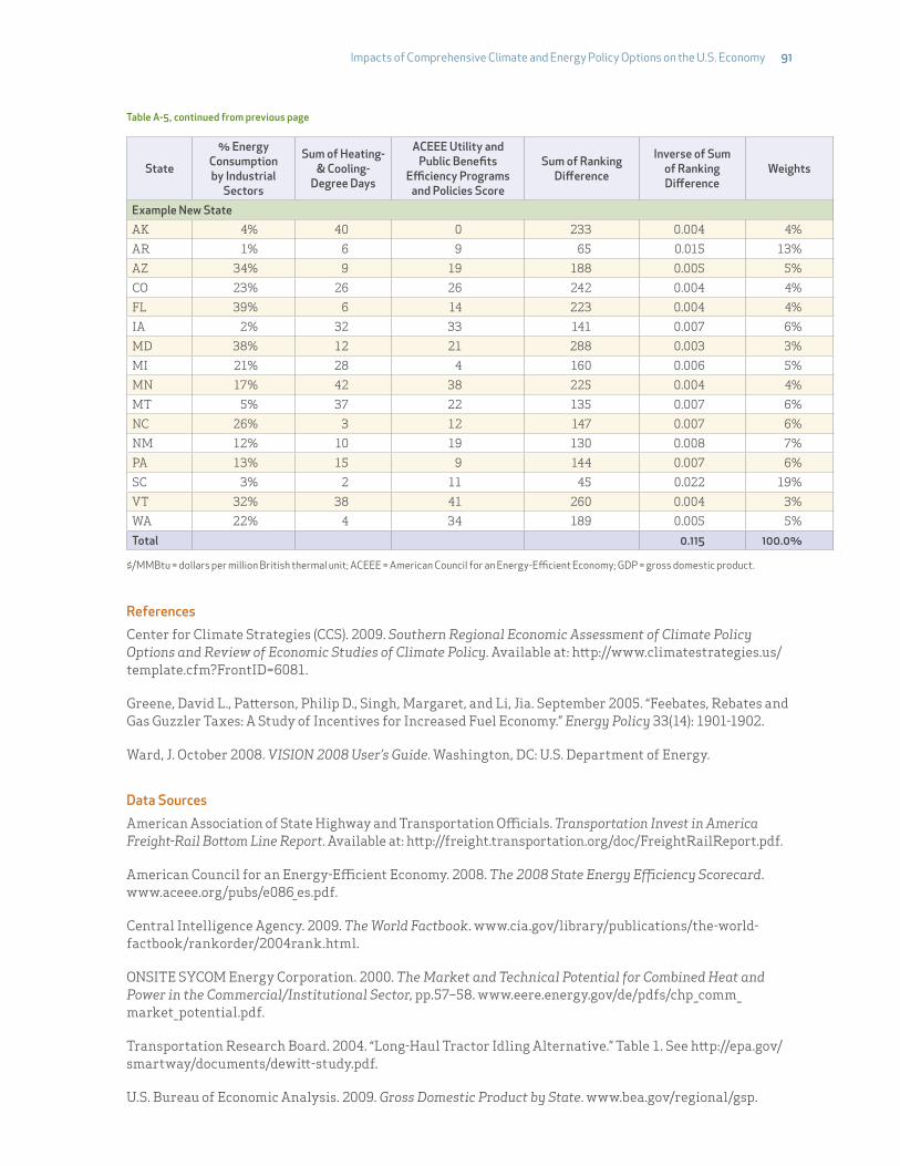
Table A-5 computes for each variable the absolute value of the ranking difference between an example new state and each of the 16 existing states. The ranking differences of all the variables are then added up in the Sum of Ranking Difference column.

In the Analogous State Method, since South Carolina has the lowest sum of ranking differences (45) across the 10 key variables with the example new state, South Carolina is selected as the analogous state for the new state for the Demand Side Management Programs option.

In the Weighted-Average Method, the Inverse of the Sum of Ranking Difference is computed for each existing state, as shown in the second-to-last column in Table A-5. The sum in this column in this case is 0.115. Then each of the inverse numbers and their sum (0.115) in this column are used to compute the weights, as shown in the last column of Table A-5. Intuitively, this approach assigns higher weights to existing states that have comparatively less differences with the new state. These weights will then be used in the 16-state Weighted-Average Method to estimate the GHG reduction potentials and cost-effectiveness of the Demand Side Management Programs option for the new state. This mathematical approach attempts to quantify similarities between individual states by comparing how each state ranks relative to others. For example, for electricity-exporting states, the weighting methodology allows for estimates of GHG reduction supplies to be more heavily weighted with data from states like New Mexico and Montana, the largest electricity exporters in the existing 16-state database.


Table A-4. Key Factors for the Demand Side Management Programs Option

States

Per Capita Income ($)

Per Capita Electricity

Consumption (megawatt-hours)

Net Electricity Trade Index

[= production / (consumption +

losses)]

Weighted-Average Delivered Electricity

Price (cents/kilowatt-hour)

Weighted-Average

Natural Gas Price ($/MMBtu)

% GDP from Manufacturing

Sector

Value Ranking Value Ranking % Ranking Value Ranking Value Ranking % Ranking

States Without Action Plans

AL 32,419 44 20.3 3 1.39 8 7.57 28 9.8 24 17.22% 10

CA 43,641 8 7.3 50 0.72 44 12.80 10 8.7 38 9.81% 33

CT 56,272 1 9.7 40 0.94 31 16.45 2 11.0 15 13.35% 18

DE 40,519 18 14.2 24 0.61 48 11.35 13 10.8 17 7.39% 40

GA 33,499 40 15.4 16 0.94 31 7.86 25 11.5 8 10.88% 26

HI 42,055 14 8.3 47 0.99 25 21.29 1 26.8 1 1.71% 50

ID 33,074 43 16.9 11 0.44 50 5.07 50 9.5 27 9.86% 31

IL 42,347 13 11.5 36 1.25 12 8.46 21 9.9 23 12.43% 21

IN 34,605 36 17.5 9 1.06 18 6.50 42 9.2 30 25.03% 1

KS 38,820 22 14.6 23 1.14 16 6.84 39 9.1 32 15.15% 14

KY 30,824 47 22.2 2 0.97 29 5.84 47 10.9 16 18.43% 6

LA 35,100 32 17.5 8 0.85 38 8.39 22 7.6 45 18.25% 7

MA 51,254 3 8.8 45 0.77 43 15.16 4 12.2 6 9.54% 35

ME 36,457 29 9.0 44 1.20 13 14.59 5 8.9 36 11.05% 25

MO 33,964 38 14.8 21 0.99 25 6.56 41 12.3 5 13.48% 17

MS 28,541 50 16.5 13 0.92 33 8.03 23 8.6 39 14.96% 15

ND 39,870 20 18.7 6 2.30 3 6.42 43 7.6 44 9.08% 37

NE 39,150 21 16.2 14 1.05 19 6.28 46 9.0 34 11.84% 23

NH 43,623 9 8.5 46 1.87 4 13.98 6 10.3 21 10.86% 27

NJ 51,358 2 9.4 42 0.69 46 13.01 9 11.3 13 9.23% 36

NV 41,182 17 15.2 19 0.85 38 9.99 16 8.1 42 4.37% 46

NY 48,753 4 7.7 48 1.00 23 15.22 3 11.4 10 6.04% 43

OH 36,021 31 14.1 25 0.89 35 7.91 24 11.4 12 17.83% 8

OK 34,997 33 15.7 15 1.18 14 7.29 31 8.1 43 10.75% 28

OR 36,297 30 13.5 28 1.05 19 7.02 36 9.0 33 18.69% 5

RI 41,368 16 7.4 49 0.87 37 13.12 8 10.7 18 9.82% 32

SD 38,661 24 13.7 27 0.53 49 6.89 38 8.9 37 9.57% 34

TN 33,395 42 17.9 7 0.82 41 7.07 35 11.6 7 16.10% 12

TX 37,083 28 15.1 20 1.02 21 10.11 15 7.0 47 12.98% 19

UT 31,944 45 11.5 37 1.45 7 6.41 44 7.2 46 11.86% 22

VA 41,727 15 14.8 22 0.65 47 7.12 34 11.5 9 8.59% 38

WI 37,767 26 12.8 32 0.80 42 8.48 20 10.2 22 20.32% 3

WV 29,385 49 18.8 5 2.48 2 5.34 48 11.2 14 10.73% 29

WY 48,608 5 30.6 1 2.56 1 5.29 49 7.0 48 3.06% 48

States With Action Plans

AK 44,039 7 9.6 41 0.97 29 13.28 7 5.8 50 1.99% 49

AR 30,177 48 16.9 10 1.02 21 6.96 37 9.0 34 17.37% 9

AZ 34,335 37 13.2 31 1.33 10 8.54 18 8.4 40 7.85% 39

CO 42,985 11 11.1 38 0.99 25 7.76 27 6.9 49 6.40% 42

FL 38,417 25 13.2 29 0.89 35 10.33 14 9.1 31 4.80% 45

IA 37,402 27 15.2 17 1.00 23 6.83 40 9.5 28 20.76% 2

MD 46,471 6 11.7 35 0.70 45 11.50 12 13.3 2 5.56% 44


States

Per Capita Income ($)


Consumption (megawatt-hours)



losses)]

Weighted-Average Delivered Electricity

Price (cents/kilowatt-hour)

Weighted-Average

Natural Gas Price ($/MMBtu)

% GDP from Manufacturing

Sector

Value Ranking Value Ranking % Ranking Value Ranking Value Ranking % Ranking

MI 34,949 34 10.7 39 0.98 28 8.53 19 9.6 26 16.14% 11

MN 43,037 10 13.2 30 0.84 40 7.44 29 9.3 29 12.83% 20

MT 34,644 35 16.6 12 1.50 5 7.13 33 9.6 25 4.05% 47

NC 33,735 39 15.2 18 0.90 34 7.83 26 12.3 4 19.48% 4

NM 33,430 41 11.7 34 1.50 5 7.44 29 8.4 41 6.59% 41

PA 40,140 19 12.2 33 1.37 9 9.08 17 11.4 10 13.64% 16

SC 31,103 46 19.3 4 1.16 15 7.18 32 10.3 20 16.10% 13

VT 38,686 23 9.3 43 1.30 11 12.04 11 12.7 3 11.40% 24

WA 42,857 12 13.8 26 1.12 17 6.37 45 10.5 19 9.91% 30

States

% Energy Consumption by Residential & Commercial

Sectors

% Energy Consumption by Industrial Sectors

Sum of Heating- & Cooling-Degree Days

ACEEE Utility and Public Benefits Efficiency Programs and Policies Score

(Maximum Possible Points Is 20)

% Ranking % Ranking Value Ranking Value Ranking

States Without Action PlansAL 32% 42 45% 9 4,537 43 0.0 42

CA 37% 33 23% 37 1,968 50 14.5 3

CT 56% 3 14% 45 6,863 16 15.5 2

DE 40% 25 35% 18 6,012 27 0.0 42

GA 40% 24 29% 28 4,463 46 1.5 31

HI 24% 47 21% 40 4,561 42 8.5 14

ID 39% 31 36% 16 6,578 19 10.0 10

IL 43% 17 30% 27 7,328 14 3.0 25

IN 30% 44 47% 6 6,563 20 2.5 28

KS 39% 32 35% 17 6,423 22 1.0 33

KY 30% 43 46% 8 5,604 32 3.0 25

LA 16% 50 64% 1 4,288 48 0.0 42

MA 54% 5 14% 46 6,407 23 12.5 6

ME 39% 28 32% 24 7,672 9 6.5 18

MO 46% 11 23% 38 5,991 29 0.0 42

MS 32% 40 37% 15 4,483 44 0.0 42

ND 28% 45 49% 4 9,280 2 0.5 38

NE 42% 20 31% 25 7,407 12 0.5 38

NH 52% 7 15% 44 7,927 7 7.5 17

NJ 45% 14 17% 42 6,048 26 10.0 10

NV 40% 26 27% 33 6,094 25 8.5 14

NY 60% 1 12% 50 7,405 13 12.5 6

OH 40% 27 34% 20 6,253 24 5.5 21

OK 34% 36 38% 13 5,015 38 0.0 42

OR 43% 16 26% 34 4,764 41 13.5 4

RI 58% 2 12% 49 6,468 21 10.0 10

SD 43% 15 24% 36 8,503 4 0.5 38

TN 39% 29 33% 23 5,138 36 1.0 33

TX 25% 46 50% 3 4,430 47 3.0 25

UT 39% 30 28% 29 6,696 18 6.5 18

VA 46% 12 22% 39 5,308 35 1.0 33

WI 41% 21 35% 19 7,712 8 10.0 10



States


Sectors

% Energy Consumption by Industrial Sectors

Sum of Heating- & Cooling-Degree Days

ACEEE Utility and Public Benefits Efficiency Programs and Policies Score

(Maximum Possible Points Is 20)

% Ranking % Ranking Value Ranking Value Ranking

WV 32% 41 46% 7 5,984 30 0.0 42

WY 21% 48 53% 2 7,569 10 0.0 42

States With Action PlansAK 17% 49 48% 5 8,574 3 0.0 42

AR 34% 37 41% 10 5,021 37 1.0 33

AZ 49% 8 15% 43 5,395 34 4.0 23

CO 42% 18 27% 32 6,823 17 8.0 16

FL 52% 6 13% 48 4,085 49 2.5 28

IA 34% 38 41% 11 7,484 11 10.5 9

MD 55% 4 13% 47 5,618 31 5.5 21

MI 45% 13 28% 30 7,176 15 0.5 38

MN 41% 23 31% 26 9,931 1 13.5 4

MT 34% 35 38% 14 8,001 6 6.0 20

NC 47% 10 26% 35 4,780 40 2.0 30

NM 33% 39 33% 21 5,571 33 4.0 23

PA 41% 22 33% 22 5,994 28 1.0 33

SC 35% 34 38% 12 4,467 45 1.5 31

VT 48% 9 19% 41 8,154 5 19.0 1

WA 42% 19 27% 31 4,970 39 12.0 8

ACEEE = American Council for an Energy-Efficient Economy; $/MMBtu = cost per million British thermal unit; GDP = gross domestic product.

Table A-5. Ranking Differences of Relevant Variables for the Demand Side Management Programs Option: An Example of a New State Versus 16 Existing States

State Per Capita Income ($)


Consumption (megawatt-

hours)



losses)]

Weighted-Average Delivered

Electricity Price (cents/kilowatt-

hour)

Weighted-Average

Natural Gas Price

($/MMBtu)

% GDP From Manufacturing

Sector


Sectors

Example New State

AK 37 38 21 21 26 39 7

AR 4 7 13 9 10 1 5

AZ 7 28 2 10 16 29 34

CO 33 35 17 1 25 32 24

FL 19 26 27 14 7 35 36

IA 17 14 15 12 4 8 4

MD 38 32 37 16 22 34 38

MI 10 36 20 9 2 1 29

MN 34 27 32 1 5 10 19

MT 9 9 3 5 1 37 7

NC 5 15 26 2 20 6 32

NM 3 31 3 1 17 31 3

PA 25 30 1 11 14 6 20

SC 2 1 7 4 4 3 8

VT 21 40 3 17 21 14 33

WA 32 23 9 17 5 20 23



State

% Energy Consumption by Industrial

Sectors

Sum of Heating- & Cooling-

Degree Days

ACEEE Utility and Public Benefits

Efficiency Programs and Policies Score

Sum of Ranking Difference

Inverse of Sum of Ranking Difference

Weights

Example New State

AK 4% 40 0 233 0.004 4%

AR 1% 6 9 65 0.015 13%

AZ 34% 9 19 188 0.005 5%

CO 23% 26 26 242 0.004 4%

FL 39% 6 14 223 0.004 4%

IA 2% 32 33 141 0.007 6%

MD 38% 12 21 288 0.003 3%

MI 21% 28 4 160 0.006 5%

MN 17% 42 38 225 0.004 4%

MT 5% 37 22 135 0.007 6%

NC 26% 3 12 147 0.007 6%

NM 12% 10 19 130 0.008 7%

PA 13% 15 9 144 0.007 6%

SC 3% 2 11 45 0.022 19%

VT 32% 38 41 260 0.004 3%

WA 22% 4 34 189 0.005 5%

Total 0.115 100.0%

$/MMBtu = dollars per million British thermal unit; ACEEE = American Council for an Energy-Efficient Economy; GDP = gross domestic product.

References

Center for Climate Strategies (CCS). 2009. Southern Regional Economic Assessment of Climate Policy Options and Review of Economic Studies of Climate Policy. Available at: http://www.climatestrategies.us/template.cfm?FrontID=6081.

Greene, David L., Patterson, Philip D., Singh, Margaret, and Li, Jia. September 2005. “Feebates, Rebates and Gas Guzzler Taxes: A Study of Incentives for Increased Fuel Economy.” Energy Policy 33(14): 1901-1902.

Ward, J. October 2008. VISION 2008 User’s Guide. Washington, DC: U.S. Department of Energy.

Data Sources

American Association of State Highway and Transportation Officials. Transportation Invest in America Freight-Rail Bottom Line Report. Available at: http://freight.transportation.org/doc/FreightRailReport.pdf.

American Council for an Energy-Efficient Economy. 2008. The 2008 State Energy Efficiency Scorecard. www.aceee.org/pubs/e086_es.pdf.

Central Intelligence Agency. 2009. The World Factbook. www.cia.gov/library/publications/the-world-factbook/rankorder/2004rank.html.

ONSITE SYCOM Energy Corporation. 2000. The Market and Technical Potential for Combined Heat and Power in the Commercial/Institutional Sector, pp.57–58. www.eere.energy.gov/de/pdfs/chp_comm_market_potential.pdf.

Transportation Research Board. 2004. “Long-Haul Tractor Idling Alternative.” Table 1. See http://epa.gov/smartway/documents/dewitt-study.pdf.

U.S. Bureau of Economic Analysis. 2009. Gross Domestic Product by State. www.bea.gov/regional/gsp.


http://www.aceee.org/pubs/e086_es.pdf

http://www.aceee.org/pubs/e086_es.pdf

https://www.cia.gov/library/publications/the-world-factbook/rankorder/2004rank.html



http://www.eere.energy.gov/de/pdfs/chp_comm_market_potential.pdf

http://www.eere.energy.gov/de/pdfs/chp_comm_market_potential.pdf


U.S. Bureau of Economic Analysis and Bureau of the Census. 2008. State Personal Income 2008. www.bea.gov/newsreleases/regional/spi/spi_newsrelease.htm.

U.S. Bureau of the Census, Population Division. 2004. State Interim Population Projections by Age and Sex: 2004–2030. www.census.gov/population/www/projections/projectionsagesex.html.

U.S. Bureau of the Census. 2009. Heating- and Cooling-Degree Days. www.census.gov/compendia/statab/tables/09s0379.xls.

U.S. Department of Energy, http://www.afdc.energy.gov/afdc/locator/tse/state.

U.S. Department of Energy, Energy Information Administration. 2005. 2002 Energy Consumption by Manufacturers. http://www.eia.doe.gov/emeu/mecs/mecs2002/data02/shelltables.html.

U.S. Department of Energy, Energy Information Administration. 2008. State Energy Data System. www.eia.doe.gov/emeu/states/hf.jsp?incfile=sep_sum/plain_html/sum.

U.S. Department of Energy, Energy Information Administration. 2009. Electric Power Annual 2007. www.eia.doe.gov/cneaf/electricity/epa/epa_sprdshts.html.

U.S. Department of Energy, Energy Information Administration. 2009. State Electric Profile. www.eia.doe.gov/cneaf/electricity/st_profiles/e_profiles_sum.html.

http://www.bea.gov/newsreleases/regional/spi/spi_newsrelease.htm

http://www.bea.gov/regional/gsp/

http://www.bea.gov/regional/gsp/

http://www.census.gov/population/www/projections/projectionsagesex.html

http://www.census.gov/population/www/projections/projectionsagesex.html

http://www.census.gov/compendia/statab/tables/09s0379.xls






http://www.eia.doe.gov/emeu/states/hf.jsp?incfile=sep_sum/plain_html/sum

http://www.eia.doe.gov/emeu/states/hf.jsp?incfile=sep_sum/plain_html/sum

http://www.eia.doe.gov/cneaf/electricity/epa/epa_sprdshts.html. 5

http://www.eia.doe.gov/cneaf/electricity/epa/epa_sprdshts.html. 5

http://www.eia.doe.gov/cneaf/electricity/st_profiles/e_profiles_sum.html

annex a: impacts of comprehensive climate and energy policy options on the u.s. economy

Documents