anisotropic acquisition and analysis for diffusion tensor...

by

Jee Eun Lee

A dissertation submitted in partial fulfillment of

the requirements for the degree of

Doctor of Philosophy

(Medical Physics)

at the

UNIVERSITY OF WISCONSIN-MADISON

2006

Anisotropic Acquisition and Analysis for Diffusion Tensor Magnetic Resonance Imaging

i ABSTRACT

Diffusion tensor magnetic resonance imaging (DT-MRI) is a noninvasive imaging

method for assessing the characteristics and organization of tissue microstructure. The

diffusion tensor provides information about the magnitude, anisotropy, and orientation of

water diffusion in biological tissues. In brain white matter, the direction of greatest

diffusivity is typically assumed to be parallel to the white matter tracts. The number of

DT-MRI applications is rapidly expanding; however, diffusion tensor measurements are

also highly sensitive to noise in the raw diffusion weighted (DW) images. Furthermore,

the relatively poor spatial resolution of most DT-MRI studies cause partial volume

averaging between different tissue regions, which can lead to errors in the estimated DT-

MRI measures. Finally, the variance of DT-MRI measures may impair the ability to

detect and characterize subtle differences either between regions or subjects. In this thesis,

new acquisition and analysis methods for reducing measurement noise effects are

investigated.

For the case where the diffusion tensor orientation and shape may be estimated a

priori, changing the diffusion-weighting with encoding direction may improve the overall

accuracy of the diffusion tensor measurements. The variance of DT-MRI measurements

is expressed as a function of directional diffusitivities and diffusion weightings.

Minimizing the variance using quadratic optimization algorithms leads to an obtainment

of anisotropic diffusion weightings. In this study anisotropic diffusion weighting reduced

the variance of FA and MD measurements by roughly 50 % in the corpus callosum.

Anisotropic Gaussian kernel smoothing was used to reduce the errors and noise for

ii the entire regions of DT-MRI data. The anisotropic Gaussian kernels for convolution

smoothing are equivalent to the water diffusion distributions described by the diffusion

tensor. Further the direction of greatest diffusitivity is often assumed to be parallel to the

direction of the local white matter tracts, thus the measured diffusion tensor is a good

candidate for anisotropic kernel smoothing. This reduces the partial averaging effects

with high levels of smoothing.

In voxel based analyses of DT-MRI data, isotropic Gaussian kernel smoothing is

often used to blur the individually distinct anatomic features. Anisotropic Gaussian kernel

smoothing may reduce the partial volume averaging which will improve anatomic

specificity. In this study, anisotropic Gaussian smoothing was applied to DT-MR data

from a group of autism subjects to investigate the differences of DT-MRI measurements

between the autism and control groups. Anisotropic Gaussian kernel smoothing provides

more consistent results for the group differences as compared with manual ROI analysis

Finally, anisotropic Gaussian kernel smoothing may be useful for estimating anatomic

connectivity as the diffusion will be greatest along the white matter pathways. In this

study iterative convolution with anisotropic Gaussian kernels was used to estimate

connectivity patterns in DT-MRI fields. Preliminary results in both phantoms and human

brain were promising. Future developments will constrain the diffusion propagation to

white matter to eliminate erroneous pathways.

iii

Acknowledgments

First and foremost, I would like to thank my supervisor Andy Alexander for his

warm and insightful guidance. His continuing devotion and innovative ideas in his

studies have been truly inspiring to me.

I am thankful for Moo Chung for his exquisite knowledge and useful advice in

Statistics. Without his abundant ideas and guidance, my thesis would not be carried on in

a right direction. I’d also like to thank all my other committee members; Beth Meyerand,

Wally Block, and Aaron Field, who generously advised me to carry out this dissertation.

I would not be able to accomplish what I wanted without Terry Oakes and Mariana

Lazar for all my computer programming troubles. I’d like to send my great appreciation

to Mariana and Terry for their valuable help.

I am sincerely grateful to Prof. Hyun Myung Jang, who always believes in me and

guides me. I’d like to thank all my friends to cheer me up whenever I got desperate,

especially Hyejeen Lee and Jeihoon Baek to have helped me grow as a person.

Last but not least, I thank my parents and my sisters who love and support me in

every way.

iv

Contents

1 Outlook ………………………………………………………….................. 1

2 Diffusion tensor magnetic resonance imaging ……………….................. 2

2.1 Introduction ……………………..................................................... 2

2.2 Magnetic resonance signal in Block equation …………………… 5

2.3 Signal detection and MRI reconstruction …………………………... 8

2.4 Diffusion ………………………………........................................... 10

2.5 Modified Block equation with diffusion and DT-MRI ................... 11

3 Optimization of diffusion tensor encoding with anisotropic diffusion weighting

………………………………….................................................................. 16

3.1 Introduction …………………………………......................... 16

3.2 Theory …………………………………......................... 17

3.3 Methods …………………………………………………. 20

3.4 Results …………………………………………………. 22

3.5 Conclusions ………………………………….......................... 24

v 4 Anisotropic Noise Filtering for DT-MRI ………………….............. 28

4.1 Introduction ………………………………………….. 28

4.2 Theory ………………………………………….. 30

4.3 Methods ………………………………………………….. 38

4.4 Results ………………………………………...………… 46

4.5 Discussion …………………………………........................... 50

4.6 Conclusions …………………………………........................... 52

5 Applications of Anisotropic Gaussian Smoothing: voxel-based analysis of DT-MRI

…………………………………............................................................... 53

5.1 Introduction …………………………………………………… 53

5.2 Methods …………………………………........................................ 54

5.3 Results …………………………………........................................ 61

5.4 Discussion ……………………………………………………. 69

5.5 Conclusions …………………………………………………… 73

6 Probabilistic connectivity of DT-MRI via anisotropic Gaussian kernel smoothing

…………………………............................................................................ 74

vi 6.1 Introduction …………………………………......................... 74

6.2 Theory …………………………………..................................... 76

6.3 Methods …………………………………..................................... 78

6.4 Results …………………………………...................................... 81

6.5 Discussion …………………….............................................. 86

7 Conclusions and future research plans …………………………… 91

References …………………………………........................................ 94

Appendix A …………………………………........................................ 105

Appendix B …………………………………........................................ 107

Appendix C …………………………………....................................... 109

Appendix D …………………………………....................................... 113

vii

List of Figures

2-1 Spin echo EPI pulse schematics …………………………………… 14

2-2 Stejskal-Tanner sequence …………………………………………… 15

3-1 Examples of directional sampling schemes …………………………….. 17

3-2 Plot of 2Dσ as a function of ibD …………………………………….. 18

3-3 Simulation results using the optimum diffusion weighting …………….. 22

3-4 An example of voxel based analysis using the optimum diffusion weightings

………………………………………………………………………….. 25

3-5 ROI analysis using the optimum diffusion weightings …………… 26

3-6 Examples of FA maps and FA variance maps using the optimum diffusion

weightings ……………………………………………………………… 27

4-1 The anisotropic Gaussian kernel that is projected in the x-y plane ……. 34

4-2 One dimensional Gaussian distribution as the diffusion time t increases 36

4-3 Example of smoothing kernels (x-y plane projected) for a voxel in the corpus

callosum for isotropic Gaussian kernel and anisotropic Gaussian kernel. ….. 36

4-4 A simulation to test the preservation of positive definiteness of the diffusion

tensor ………………………………………………………………….. 37

4-5 The effects of filtering on FA and MD in the whole brain …………….. 42

4-6 The effects of filtering on FA (a), (c) and MD (b) (d) in the total white matter

…………………………………………………….…..……………. 43

4-7 The effects of filtering on FA (a), (b) and MD (c) ,(d) in the total grey matter

……………………………………………………………………… 44

viii 4-8 Examples of filtered images of human data ………………………….. 45

4-9 Examples of filtered images of simulated data …………………… 48

4-10 The effects of filtering on FA and MD in the whole brain region with synthetic

noise added …………………………………………………………… 49

5-1 Examples of the white matter segmentation …………………………… 56

5-2 White matter segmentation: an additional removal of voxels using MD histogram

…………………………………………………………………………… 57

5-3 The corpus callosum segmentation …………………………………… 58

5-4 The regional corpus callosum segmentation …………………………… 59

5-5 Isotropic kernel smoothing with FWHM 12 mm. vs. anisotropic Gaussian kernel

smoothing 12 mm …………………………………………………… 62

5-6 Examples of histograms of data from isotropic smoothing vs. anisotropic

smoothing …………………………………………..………………. 63

5-7 t-maps of FA masked from a 12 mm FWHM isotropic Gaussian kernel smoothing and

with a 12 mm FWHM anisotropic kernel smoothing ………………….. 66

5-8 t-maps of MD masked from a 12 mm FWHM isotropic Gaussian kernel smoothing and

with a 12 mm FWHM anisotropic kernel smoothing ……………………….. 67

5-9 t-maps of 3λ masked from a 12 mm FWHM isotropic Gaussian kernel smoothing and

with a 12 mm FWHM anisotropic kernel smoothing ……………………….. 68

ix 5-10 Co registered white matter mask analysis: isotropic kernel smoothing with

FWHM 12 mm and FWHM 4 mm …………………………………. 71

5-11 Co registered white matter mask analysis: anisotropic kernel smoothing with

FWHM 12 mm and FWHM 8 mm …………………………………. 72

6-1 A numerical phantom with matrix size (100,100,100), FA map of the central

coronal view …………………………………………………………. 78

6-2 The x-y plane view of the kernel of a numerical phantom ………… 79

6-3 Examples of Gaussian kernels in the corpus callosum with different powers for

the diffusion tensor ………………………………………………… 80

6-4 Examples of the convolution smoothing with a seed situated in the numerical

phantom …………………………………………………………. 83

6-5 Examples of effects from using different powers of the diffusion tensor for a

numerical phantom …………………………………………………. 84

6-6 Examples of the convolution smoothing with a seed situated in the splenium of

the corpus callosum ………………………………………………. 85

6-7 Numerical simulation for the KL distance ………………………. 88

6-8 An examples of the KL distance with a seed situated in the splenium of the corpus

callosum ……………………………………………………….. 89

x

List of Tables

2-1 Properties of some NMR-Active Nuclei …………………………… 6

2-2 Typical brain tissue parameters measured at 1.5T …………………... 7

3-1 Encoding directions, average diffusitivities from ROI, their standard deviation,

and optimum diffusion weightings …………………………………………… 23

5-1 Group Comparison of Anisotropy and Diffusivities in the Corpus Callosum

Determined by One-way ANOVA ……………………………………………. 64

xi

List of Symbols

ADC Apparent diffusion coefficient

AG Anisotropic Gaussian

IG Isotropic Gaussian

PM Perona Malik algorithm

B Magnetic field

b diffusion weighting

CC Corpus Callosum

CNS Central nervous system

CSF Cerebral spinal fluid

DNR Diffusion to noise ratio

DW Diffusion weighted

DWI Diffusion weighted images

DT-MRI Diffusion tensor magnetic resonance imaging

DTI Diffusion tensor imaging

EPI Echo Planar Imaging

FA Fractional anisotropy

g Diffusion weighting gradient

GM Grey matter

MD Mean Diffusitivity

NEX Number of excitations

NMR Nuclear magnetic resonance

xii RMSE Root mean squared error

ROI Region of Interest

SNR Signal to noise ratio

TE Echo time

TR Repetition time

VBM Voxel-based morphometry

WM White matter

WMT White matter tractography

1

CHAPTER 1

OUTLOOK

The Diffusion tensor (DT) is a model-based approach of describing the molecular

diffusion displacement in a three-dimensional biological medium. Diffusion tensor MRI

(DT-MRI) is a non-invasive method for mapping the diffusion properties in vivo. DT-

MRI provides information about the magnitude and anisotropy of water diffusion in

biological tissues. The simplicity of the DT model is extremely promising for a broad

range of clinical and research applications; however, one caution should be used as DT-

MRI is exceptionally sensitive to the noise in the acquired diffusion weighted (DW)

images. This dissertation introduces and describes novel methods for reducing the effects

of image of noise in DT-MRI and potential applications of anisotropic Gaussian filter

construction. Anisotropic methods for the acquisition and analysis of DT-MRI are

discussed. These approaches are promising for reducing the effects of noise in the

computed DT-MRI maps. Further, potential applications of anisotropic image analysis

are discussed. An outline summary of this thesis is described here.

Chapter 2 reviews fundamental MRI physics and introduces DT-MRI.

Formulations of detecting MR signal based on the Block equation and imaging principles

are summarized in brief. The phenomenon of water diffusion in biological tissues is

2 discussed and the methodology of DT-MRI is described.

Chapter 3 introduces a method to minimize the errors in DT-MRI measures by

modifying the diffusion weighting as a function of diffusion encoding direction; thus the

diffusion-weighting is anisotropic. The basic mathematical formulation is based on a

model of noise propagation. The multivariate variables for this optimization problem are

the directional diffusitivities from a set of user-defined diffusion sensitizing gradients.

The propagated error in the variance of diffusion tensor measurements can be minimized

if these directional diffusitivities are known a priori since the variance of diffusion tensor

measurements (fractional anisotropy or mean diffusitivity) is a function of directional

diffusitivities. In fact, the expression of co-variance of FA in terms of directional

diffusitivity measurements is the core of this chapter.

Chapter 4 compares several spatial filtering methods for DT-MRI data. The

problem of spatial filtering in a tensor field image has not been widely explored to date in

the DT-MRI literatures. In this study, isotropic Gaussian smoothing is compared with two

anisotropic smoothing methods including a new approach which uses a blurring kernel

based upon the local diffusion tensor. The performance of these filters for reducing errors

(noise and bias) in DT-MRI maps is compared in both measured in vivo human brain

data and synthetic DT-MRI data.

Chapter 5 introduces an application of anisotropic Gaussian smoothing for voxel-

based methods for DT-MRI group analysis. The method was applied to DT-MRI data

from a group of autism spectrum subjects compared with normal control subjects. In

typical voxel-based analysis, isotropic Gaussian blurring is applied to improve spatial co-

alignment between images and application of random field theory. In this study,

3 anisotropic Gaussian blurring was used to minimize the mixing of signals between

anatomical structures. The results from anisotropic smoothing show more consistency

with the results with ROI analysis in the corpus callosum.

Chapter 6 discusses another application of the anisotropic Gaussian kernel

smoothing for mapping anatomic brain connectivity. In this approach Gaussian

convolution is assumed to be a local approximation of the solution to the diffusion

equation (also called the heat equation), a method for diffusion propagation that is

estimated from the DT-MRI data. A simulation of physical diffusion phenomenon based

upon the measured diffusion tensor gives a connection probability to every voxel in the

three-dimensional data. A transitional probability value at each voxel may be considered

as a likelihood of reaching each voxel from a starting point of the propagation.

Chapter 7 summarizes the key observations from all chapters and discusses

potential future directions.

4

CHAPTER 2

DIFFUSION TENSOR MAGNETIC RESONANCE IMAGING

2.1 Introduction

This chapter reviews the fundamentals of magnetic resonance imaging (MRI) and

introduces the theory and methods for diffusion tensor magnetic resonance imaging (DT-

MRI).

Nuclear magnetic resonance (NMR) was first illustrated by F. Block and E. M.

Purcell in 1946. NMR is achieved by exciting nuclei in an externally applied magnetic

field. The detectable MR (N is usually dropped from NMR since many people are

alarmed by the word “nuclear”) signal is not created by a single nucleus but by an

enormous number of nuclei- an ensemble. This ensemble driven phenomenon allows us

to demonstrate and to study the MR phenomenon via classical vector models without

having to resort to partial-differential wave equations in modern quantum mechanics.

MR has been utilized in many fields of science. One of the most successful

applications of MR is magnetic resonance imaging (MRI)- sometimes called the most

innovative medical diagnosis tools.

In the following sections, MR signal detection, image reconstruction, and diffusion

are reviewed.

5

2.2 Magnetic resonance signal in Block equation

The spin angular momentum of a nucleus with a spin number ½ (see the Table 2-1)

has two energy states (+1/2, and -1/2). Each nuclei magnetic moment µr

in the presence

of an applied magnetic filed is governed by the relationship of (2-1)

Brrr

×= µτ (2-1)

where Br

represents the magnetic field strength, and τr

is the torque experienced by the

magnetic moment µr

. Thermo-mechanics can help us to detect that a portion of the net

∑ µr

is in the direction of the applied field Br

, and the resultant magnetic moment per unit

volume can be symbolized as magnetization Mr

. The time dependent behavior of Mr

in

the presence of an applied magnetic filed can be derived as in (2-2) using dtJdr

r=τ and

Jrr

γµ =

BMdtMd rrr

×= γ (2-2)

The Bloch equation (2-2) describes that the vector dtMdr

is always oriented

perpendicular to the plane of Br

and Mr

, which leads to the precession movement of Mr

with the precession rate being dependent on the strength of the magnetic field Br

. This

unique angular frequency of nuclear precession is called Larmor frequency 0ω

ω0 = γ B0 (2-3)

6

Table 2-1. Properties of some NMR-Active Nuclei [Liang and Lauterbur, 1999]

Nucleus Spin Relative Sensitivity Gyromagnetic Ratio (MHz/T)

1H 1/2 1.000 42.58 13C 1/2 0.016 10.71 19F 1/2 0.870 40.05 31P 1/2 0.093 11.26

Usually the total magnetic field is composed of three components [Nishimura,

1996]

( )( )10

,,

)(10

BrGkBBMdtMd

dtMd

BGBB

rrrrrrr

+⋅++×=

+

δγ

δ

(2-4)

The gradient field Gr

is essential to creating 2D or 3D images and always in the z

direction, parallel to the 0Br

. The gradient field is discussed in the next section. 1Br

is a

shot-time varying magnetic field that is perpendicular to the 0Br

Relaxation is an important descriptive parameter for the time evolution of

magnetization in the two directions. When a 1Br

field at the Larmor frequency is applied to

the system, the magnetization is perturbed and flipped in the classical vector models. The

perturbed magnetization shortly recovers the equilibrium. The recovery time frame is

unique for the object of nuclei ensemble, and can be characterized with two parameters.

The first parameter, T1, describes the spin- lattice relaxation, or longitudinal relaxation. It

7 is mathematically described by:

1

0)()(T

MtMdt

tMd zz −−=

r (2-5)

where )(tMz is the longitudinal magnetization at time t and 0M is the initial longitudinal

magnetization.

The second parameter, T2, describes the spin-spin relaxation or the transverse

relaxation. The characteristic decay time T2 causes the transverse magnetization TM that

is perpendicular to the main magnetic field to relax back to zero by dephasing the

individual spins :

2

)()(T

tMdt

tMd TT −=r

(2-6)

Table 2.2 Typical brain tissue parameters measured at 1.5 T [Vlaardingerborek and Boer]

: ρ is the proton density

Tissue T1(ms) T2(ms) relative ρ

White matter 510 67 0.61 Gray matter 760 77 0.69 Cerebrospinal fluid 2650 280 1.00

8 These two relaxation phenomena are the main source for the detectable MR signal,

and are derived by Eqn (2-5) and (2-6) in the assumption of a homogeneous external

magnetic field. The field inhomogeneiy which is often problematic for brain imaging

causes additional signal attenuation. This is parameterized by the relaxation time T2*. T2*

is proportional to T2 and is also dependent on the field inhomogeneity. By combining (2-

5) and (2-6) the Block equation becomes:

dr M dt

= γr

M × B −M x

r i + M y

r j

T2

−(M z − M z

0)r k

T1

(2-7)

2.3 Signal detection and MRI reconstruction

MR signal detection is based on Faraday’s law of electromagnetic induction and

the principle of reciprocity. The time varying magnetic flux through a conduction loop,

i.e. a receiver coil will induce an electromagnetic field in the coil.

The magnetic flux through the coil by r

M (r r ,t) is given by

Φ(t) =

r B r(

r r )

object∫ ⋅

r M (

r r ,t ) d

r r (2-8)

According to Faraday’s law of induction, the voltage V (t) induced in the coil is

V (t) = −

∂Φ(t)∂t

= −∂∂t

r B r(

r r )

object∫ ⋅

r M (

r r ,t) d

r r (2- 9)

9 If the receiver coil has a homogeneous reception field over the region of interest,

as is often assumed, the signal expression can be fur ther simplified

rderMtS trixy

object

rrr r)()0,()( ω∆−∫= (2-10)

where tt ⋅∆ )(ω is the phase accumulation due to the frequency shift from 0ω .

The gradient field Gr

relates specifically to the spin frequency at an object location,

namely, rr

:

rGrrr

⋅+= γωω 0 (2-11)

Measured with respect to the echo time TE, t’=t-TE

∫ +=+=t

xyxyyn xkykxtGyTGdttyx0

, ),,( γγω (2-12)

∫=='

0

)(t

ynyyny dttGTGk γγ (2-13)

∫=='

0

)('t

xxx dttGtGk γγ (2-14)

These xk ,and yk define k-space. Expanding (2-10) with (2-11) through (2-14), the signal

can be expressed as a function of xk ,and yk (2-15)

dxdyeyxtS ykxki

object

yx )(2),()( +−∫∝ πρ (2-15)

10

2.4 Diffusion

Diffusion refers to a macroscopic manifestation of Brownian motion, which was

first studied by Robert Brown in the early 19th century. The Brownian motion refers to

the random movement of particles in a medium, and the trajectories of the motion are

continuous. If the motion is described in a discrete fashion, it may be called as random

walk process.

One way of mathematically relating Brownian motion to the diffusion equation is

summarized in the Appendix A. A derivation of the diffusion equation from a random

walk is discussed in the Appendix B. Those two approaches (Appendix A and B)

constitute the background theory for the Chapter 6: probabilistic connectivity via

diffusion process.

The diffusion equation can also be obtained using Fick's law that relates the bulk

diffusion flux Jr

to the concentration gradient C∇ through an apparent bulk diffusion

coefficient D .

CDJ ∇−=r

, C : the concentration gradient (2-16)

Combining the Fick’s law (2-16) with the equation of conservation of mass Eqn.

(2-17),

tC

J∂∂

−=⋅∇r

(2-17)

11 The diffusion equation is obtained as

)( CDtC

∇⋅∇=∂∂

(2-18)

One solution to the diffusion equation is given by the Gaussian function

−⋅−−

=

Dtrrrr

DttrC

4)()(

exp4

1),( 00

3 rrr

π (2-19)

in which, the diffusion coefficient D may be theoretically derived. This was done by

Albert Einstein using kinetic theory. D may be experimentally measured in several ways.

The next section discusses measuring D using MR experiments.

2.5 Modified Block equation with diffusion and DT-MRI

Diffusion tensor magnetic resonance imaging (DT-MRI) is built on the assumption

that three-dimensional diffusion phenomenon of water molecular ensembles can be

assessed and described with diffusion tensor on a voxel basis. The diffusion tensor has

been proved to be a particularly successful and useful model in brain imaging for

describing the microstructure of the biological tissues using MR imaging.

As already mentioned in the previous section, the NMR phenomenon is created by

an ensemble of nuclei. Thermal physics tells us that the particles are always thermally

agitated and the associated kinetic energy is proportional to the environmental

temperature. Therefore, if the temperature is not at absolute zero, the system is not static.

12 Since anything we can measure in reality exists at some temperature above zero the

Block equation should involve the diffusion considerations.

A noninvasive method for measuring diffusion in biological system has been done

by modeling the Block equations with diffusion motion. In a bipolar pulsed-gradient

experiment [Fig 2-2], which was developed based upon a spin echo EPI pulse sequence

[Fig 2-1], the interval of two diffusion sensitizing gradients (∆ ) leads to the added

dissipation of transverse phase by individual spin’s random displacements and the

resultant signal attenuation can be derived as follows [Stejskal and Tanner, 1965]

)()(

1

0

2

MDT

kMMT

jMiMBM

dtMd zzyx r

rrrr

r∇⋅∇+

−−

+−×= γ (2-20)

where D is the diffusion coefficient.

The solution of this equation is given by:

)')'()''(exp())(exp()1

exp()0(),(02

dttkDtktkriT

tMtrMt rrrrr∫−⋅−⋅−⋅== (2-21)

where

r k (t) = γ G(t')dt '

0

t

∫ ,

Ignoring T2 attenuation, the total magnetization ratio at time TE may be expressed

in Eqn (2-21) as

),exp()(

0

bDM

TEM −= (2-22)

where b =

r k (t') ⋅

r k (t')dt'

0

TE

∫ ,

13

If anisotropic Gaussian diffusion in 3D space is considered, a tensor model may be

employed, and the equation (2-22) above becomes

),'exp()(

0

gDgbM

TEM rr−= (2-23)

where D is a 3x3 tensor and gr is a unit vector that represents the direction of the

diffusion encoding gradient. More information on diffusion tensor formalism and its

invariant measures can be found in the Appendix C. Assuming that water molecules are

electromagnetically neutral, which leads to D being a symmetric tensor, solving the six

unknown tensor elements requires at least six different gr orientations; If more than six

encoding directions are used, Eqn (2-23) becomes an over-determined equation. That can

be solved by multivariate linear regression or nonlinear regression. In this dissertation,

all DT-MRI studies are based on twelve diffusion sensitizing encoding directions [Hasan

et al 2001a] and Eqn (2-23) was solved using the singular value decomposition with

linear regression.

In the Stejskal-Tanner scheme (Fig 2-2), commonly employed for DT-MRI

experiments, the b value (or b factor, diffusion weighting) is summarized as follows

[Mattiello et al., 1997]

),3/(222 δδγ −∆= Gb (2-24)

14 where γ is the gyromagnetic ratio, δ is the duration of the diffusion sensitizing gradient

and ∆ is the separation time of the two diffusion sensitizing gradient G.

Conventional DT-MRI uses the same b value (2-25) for each encoding direction.

Utilizing different b values per encoding direction is the subject of Chapter 3 and the

solution of the diffusion equation- the Gaussian function (2-20), is exercised in the rest of

the chapters.

Fig 2-1 Spin echo EPI pulse schematics. EPI was developed by P. Mansfield [Mansfield, 1977].

EPI is a fast MRI technique to acquire an image in only a single or very few excitations.

15

Fig 2-2. Stejskal-Tanner sequence. After a 90° RF pulse, the left side diffusion gradient G is on

over a short period δ and another RF pulse 180° is applied to precede the right side diffusion

gradient G. Two diffusion sensitizing gradients G are separated by the time interval∆ . G, δ and

∆ affect the total amount of diffusion related signal attenuation on the sampled data at the echo

time.

16

CHAPTER 3

OPTIMIZATION OF DIFFUSION TENSOR ENCODING WITH ANISOTROPIC DIFFUSION WEIGHTING

3.1 Introduction

Diffusion tensor MRI and the associated measures, such as fractional anisotropy

(FA), mean diffusitivity (MD), and eigenvector directions, are highly sensitive to image

measurement noise. The main strategy to decrease noise sensitivity is to employ

uniformly distributed diffusion encoding directions with a diffusion-weighting value that

is nearly optimum for the mean diffusivity. [Papadakis N.G et al., 1999; Jones DK et al,

1999; Armitage et al., 2001; Hasan K.M. et al., 2001] These approaches make sense for

the case where the diffusion tensor distributions and directions are arbitrary or unknown.

However, in the case where the diffusion tensor shape and orientation in a specific region

may be estimated a priori, such as in the corpus callosum, the corticospinal tract, or the

spinal cord, it may be possible to make more precise measurements in that region by

using an anisotropic diffusion-weighting scheme. In this study, the diffusion weighting

was optimized for each encoding direction to minimize the error in FA measurements of

the corpus callosum.

17

Fig 3-1 Examples of directional sampling schemes. [Le Bihan et al., 2001]. Conventionally

diffusion sensitizing encoding directions are set to be uniformly distributed and a single diffusion

weighting factor is used for all directions.

3.2 Theory

The diffusion to noise ratio (DNR) introduced by Xing et al [Xing et al., 1997] is

defined as:

D

DDNR

σ= DSNRκ= , where

)2exp(1 bD

bDD

+=κ (3-1)

where D represents the diffusitivity, b the diffusion weighting, and Dσ the standard

deviation of diffusitivity.

18

Fig 3-2. Plot of 2Dσ as a function of ibD . 2

Dσ is minimized at 1.1~ibD

The measured diffusitivity variance (Fig 3.2) can be plotted as a function of ibD ,

and the function has a global minimum at 1.1~ibD .

Since the diffusion-weighted image in each direction is considered to be

independent in the diffusion tensor-encoding scheme, the DNR in each direction i can be

denoted asiDiD σ/ . Consequently, an invariant function, i.e., a function of eigenvalues

can be expressed as a function of the measurement of iD . MD and FA variance

optimizations are constructed as follows.

19 MD optimization in the anisotropic scheme

The variance of MD may be expressed as:

jii DD

n

ij

n

i ij

D

n

i i

MDDD

MDD

MD 22

2

2

2 2 σσσ ∑∑∑≠

∂∂∂

+

∂∂

= (3-2)

MD is a linear summation of iD which makes the second term in (3-2) to vanish.

This means, each iD optimization, i.e. minimization of iD2σ , will lead to MD

optimization.

Since MD is the first order of diffusitivity variables iD the variance is easily

derived. It turns out to be the same as DNR calculated above since the jG ,3,2,11− in Eqn

(3-3) is a scalar factor.

3zzyyxx DDD

MD++

=3

1,3

1

1,2

1

1,1

1 ∑∑∑=

−

=

−

=

− ++=

N

jjj

N

jjj

N

jjj DGDGDG

(3-3)

FA optimization

Unlike the MD variance described above, the FA variance has a non-zero second

term in (3-2) due to the fact that FA is the second order function of iD . Detailed

derivation is described in the Appendix C.

20 If FA is expressed as a function ofDi , the variance FA has the following form.

jii DD

n

ij

n

i ij

D

n

i i

FADD

FADFA 2

22

2

2 2 σσσ ∑∑∑≠

∂∂∂

+

∂∂

= (3-4 a)

where ji

SDD

bbSji

12

0

22 0σ

σ = (Appendix C) (3-4 b)

The FA2σ is a function of diffusitivities iD and b factors ib . The highlight of this

chapter is in fact derivation of (3-4b) which shows that the covariance from two

independent directional diffusitivities is related to the diffusion weight ing factors.

Obviously if the two diffusion weighting factors are large, the covariance of the

directional diffusitivity becomes negligible.

Once the ROI is chosen, its representative iD is inserted into (3-4) then FA2σ is

expressed as a multivariate quadratic function (3-5)

Nibf iFA L1),(2 ==σ , N = number of encoding directions. (3-5)

Any multivariate minimization algorithm, such as the direction set method, which

doesn’t require derivatives, may be implemented to find the minimum FA2σ [Lee and

Alexander, 2004].

3.3 Methods

The method that was used in this study involves error/noise propagation through

Taylor expansions to calculate the error (variance) function, f=f(diffusitivities, b factors),

and a multivariate optimization algorithm to find the minimum of the error function.

21 A single-shot spin echo EPI sequence with diffusion-tensor encoding (12

directions (optimized using minimum energy criterion [Hasan et al 2001a]), & b =

1000s/mm2) was used to estimate the diffusion tensor of the corpus callosum. A region of

interest (ROI) in the corpus callosum, which is the largest white matter pathway

consisting mostly of contralateral axon projections that are made up of about 200-250

million nerve fibers, was selected manually. Only voxels with FA > 0.6 and the x

component of the major eigenvector> 0.9 retained. The measured diffusitivities of these

voxels were averaged for each encoding direction to estimate a representative set of

directional diffusitivities in the corpus callosum [Table 3-1]. Powell’s optimization

method was used to estimate the twelve directionally optimum b factors by minimizing

the variance of FA. The optimum diffusion weighting for each direction is listed in Table

1-1. Note that the optimum directional diffusion weightings ranged between 595 and

2014 s/mm2. In order to achieve the necessary diffusion weighting for the anisotropically

optimized encoding set, the times ∆ (interval between the two diffusion gradient pulses),

and δ (the diffusion gradient pulse duration) were increased from 21 ms to 26.2 ms and

from 27.4 ms to 32.2 ms, respectively. A subsequent diffusion tensor scan was

performed on the same subject using both with the isotropic diffusion-weighting (b =

1000 s/mm2) and the optimized anisotropic diffusion-weighting scheme listed in Table 3-

1. The scan was repeated nine times for each set of encoding weightings to estimate the

variance in FA for the region that was selected (FA>0.6, ex >0.9) in the corpus callosum.

22 3.4 Results

Simulation

The error propagation in simulation predicted that the variance in FA should

decrease by 56% using the anisotropic diffusion-weighting (shown in red plot, Fig 3-3).

A set of FA optimized b factors was inserted to the Eqn. (3-2) to see the impact on MD

variance. The reduction rate of the MD variance was close to the FA variance reduction

(shown in blue plot, Fig 3-3) indicating that us ing the FA optimizing b factors may be

also beneficial to optimizing MD measurements.

Fig 3-3 simulation results using the optimum diffusion weighting that are listed in the Table 3-

1.The line in green is the variance by using b=1000 s/mm2 isotropically, and the red line indicates

the variance of FA by using anisotropic b factors listed in the table 3-1. The blue line is the

consequent MD variance by using the same b factors that were optimized for FA.

23 Table 3-1. Encoding directions, average diffusit ivities from ROI, their standard deviation, and optimum diffusion weightings

Gx Gy Gz Mean (x10-3) Std dev (x10-3) FA optimized b factors

0.418 0.502 0.144 0.698 -0.090 -0.224 0.953 0.617 -0.918 -0.577 0.048 -0.735

0.824 0.568 -0.429 0.048 -0.829 -0.964 0.194 -0.166 0.354 0.740 0.276 -0.617

0.383 0.652 -0.891 -0.714 0.552 -0.142 0.234 0.769 0.180 -0.344 -0.960 0.282

0.568 1.11 0.562 0.988 0.649 0.738 1.91 1.08 1.36 0.741 0.525 1.38

0.0921 0.187 0.0458 0.220 0.0645 0.0751 0.208 0.200 0.185 0.0860 0.0737 0.156

1759 1033 1968 825 2014 1954 510 872 595 1104 1971 623

ROI based analysis

Fig 3-4 shows an example of how voxel based analysis was done. In most cases,

the FA variance was noticeably larger when using the isotropic diffusion weighting factor

of 1000 s/mm2 than when using the optimum diffusion weighting factors in the corpus

callosum area. The variance of the collection of voxels was estimated in the ROI shown

in the Fig 3-5. The ROI was manually drawn in the corpus callosum region with the same

threshold when the optimum diffusion weighting factor scheme was performed in the

method section. The x axis in the plot indicates the ROI (voxel index) and each bar

represents the standard deviation over the nine acquisition period. A significant reduction

in the variance was observed using the anisotropic diffusion weighting scheme.

In addition to the reduction of the FA variance, new optimum b factors decreased

the residual error |)lnln

(| ii

Ti

i

ioi gDg

bSS

D∑ −−

= in the corpus callosum region from ~2.5

to ~2.1. This fact ensures a better fitting to the single tensor model with the optimum b

24 factors.

Visualization of images

The optimum tensor encoding was applied to four other subjects and similar results

were obtained. Axial FA maps through the body of the corpus callosum for isotropic

diffusion weighting and the optimized anisotropic diffusion-weighting are shown in Fig

3-6. In general, the corpus callosum appears fuller and less noisy in the FA image

obtained with anisotropic diffusion-weighting. The other white matter regions, however,

appear blurrier and noisier. The variances of the FA maps across the nine runs are shown

in Fig 3-6. The variance in the corpus callosum is lower for anisotropic diffusion-

weighting but higher in most other brain regions. The overall reduction of the FA

variance in the corpus callosum region using optimum b factors was threefold.

3.5 Conclusions

Optimizing the diffusion-weighting for individual encoding directions was found to

reduce the variances of FA measurements in regions where there was an a priori estimate

of the apparent water diffusion tensor. However, as expected, in regions where the

diffusion tensor was not similar to the optimization case, the accuracy tended to be

similar or worse.

The sensitivity of the anisotropic encoding to slight variations in tensor shape and

orientation is unknown. In addition to the corpus callosum, this method may be useful

for studies of other white matter regions that are relatively homogeneous and the

25 approximate direction is known before the experiment, such as the spinal cord and the

corticospinal tract.

Fig 3-4 An example of voxel based analysis using the optimum diffusion weightings that are

listed in the table 3-1. As shown in the bottom left plot of the figure, the FA value at a voxel

fluctuates over the time series when using an isotropic diffusion weighting factor 1000 s/mm2.

Using the optimum diffusion weighting factor, FA variance was significantly reduced (bottom,

right).

26

Fig 3-5 ROI analysis using the optimum diffusion weightings that are listed in the table 3-1. Each

bar represents the standard deviation over nine time series. The standard deviation was noticeably

reduced using anisotropic diffusion weighting schemes.

27

Fig 3-6 The top row: FA maps using b= 1000 s/mm2 vs. FA map using optimum b factors listed

in the Table 3-1. The bottom row: the variance map of FA over repeated measurements using

conventional b factors vs. the variance map of FA using optimum b factors. Significantly lower

variance was observed in the CC using the anisotropic diffusion scheme.

28

CHAPTER 4

NOISE FIILTERING FOR DT-MRI

4.1 Introduction

The high sensitivity of DT-MRI to noise and error in the DW images may be

locally reduced by using the anisotropic diffusion weighting scheme discussed in the

previous chapter. However, the local error minimization from Chapter 3 is only optimal

for a specific tensor shape and orientation which must be known a priori. Therefore it

might not be useful for the whole brain assessment because its directional diffusitivity

would be different from region to region. To target the general heterogeneous region,

increasing the number of averaging DW data can substantially increase the SNR, yet in

certain cases (e.g., young children, anxious or claustrophobic subjects, etc.) it may be

desirable to minimize the acquisition time of the DT-MRI protocol. Lowering the spatial

resolution might increase the SNR, but obviously, the spatial resolution should be

improved to reduce partial volume averaging and to study the anatomy with greater detail

[Alexander et al, 2001]. Consequently, either the reduction of scan time (e.g., fewer

averages or encoding directions) or the acquisition of images with smaller voxel

dimensions will significantly reduce the SNR of DT-MRI measurements, thereby

29 affecting the accuracy. Reduced SNR will not only increase the variance of the

diffusivities, anisotropy, and eigenvector directions, but will also induce biases into the

eigenvalues and anisotropy measures [Pierpaoli and Basser, 1996; Basser and Pajevic,

2000]. The sorting bias of eigenvalues in noisy DT-MRI data causes a systematic

overestimation of the largest eigenvalues and an underestimation of the smallest

eigenvalues [Anderson, 2001].

In this chapter, a more reliable method to decrease the noise in DT-MRI through

post processing is discussed and anisotropic Gaussian smoothing using the diffusion

tensor at each voxel as the anisotropic diffusion kernel is proposed. The application of the

diffusion tensor as a convolution kernel will inherently smooth the data more in the

direction of greater diffusivity which is generally parallel to the orientation of white

matter tracts in the brain. Conversely, in gray matter areas, which demonstrate more

isotropic diffusion, the smoothing will also be more isotropic. The anisotropic kernel

smoothing approaches are compared against isotropic Gaussian smoothing and the

Perona Malik filtering algorithm. Comparisons of filtering applied directly to the

diffusion weighted data and to the estimated diffusion tensor elements are performed.

The performance of each spatial filtering method is evaluated as a function of SNR in in-

vivo high- resolution human DT-MRI data using the root mean squared error (RMSE)

that describes the accuracy and variance of the diffusion tensor measures.

30

4.2 Theory

Image filtering and smoothing methods may be used to reduce noise in medical

images. However, certain types of smoothing may also blur important image features

and the edges of structures. Fine image features and edges may be preserved using

anisotropic diffusion filtering methods such as Perona-Malik (PM) algorithm [Perona and

Malik, 1990]. Note that anisotropic diffusion here refers to the image filter used and not

the anisotropy from the diffusion tensor. The PM filter was originally developed for

scalar images and methods for smoothing DT-MRI data may require more complex

approaches than scalar image smoothing methods, because the diffusion tensor image

data is multidimensional and represents spatially coherent directional information by the

eigenvectors and eigenvalues. In this section, several smoothing algorithms are discussed:

They are the conventional isotropic Gaussian kernel, which is mostly used in the medical

image community, an anisotropic diffusion scheme using PDE to compensate for the

demerits of Gaussian blurring, and anisotropic Gaussian kernel smoothing that is based

on the measured diffusion tensor.

Gaussian kernel smoothing

Gaussian kernel smoothing is typically used in the field of image processing. The

Gaussian convolution is a linear operator and the resultant convolved image has less

noise due to the local averaging operation. The Gaussian kernel smoothing is essentially a

low pass filter in that the abrupt signal intensity change, which often time is due to noise,

is decreased thanks to the averaging with the neighborhood intensity values. The n-

31 dimensional Gaussian distribution is defined as

K(

r r ) =

exp(−r r '

r r /2σ 2)

(2π )n / 2σ n , r r = (r1,r2,L,rn )' (4-1)

where rr

is the position vector, and σ is the standard deviation of the distribution )(rKr

in

the n dimensional case.

This kernel in Eqn. (4-1) is herein called the isotropic Gaussian kernel partially

because it has an isotropic shape and also in order to be compared against an anisotropic

Gaussian kernel tha t is introduced later.

The mathematical description of Gaussian convolution is defined over the entire

domain, from - 8 to + 8, or the entire grid of points of data. However, integration of the

entire region for each data point is computationally overloaded, and in reality, the

Gaussian decreases exponentially, a reasonable approximation could be used. For

instance, integrating the kernel in the closed cube [-2.58, 2.58] leads to the value, 0.99,

which is close to 1. Therefore, a limited window size is used instead of the entire domain

and, which leads to the procedure that the kernel should be normalized in order to keep

the total probability 1, so that the kernel K is transformed as∫

=

window

KK

K~ .

To increase the kernel size, the iterated convolution is used.

tttttnKKKKK ⊗⊗⊗= ... (n times) (4-2)

32

PDE based image smoothing : Perona Malik Algorithm

Partial differential equations (PDEs), specifically the diffusion equation (hereafter,

heat equation, not to be confused with the diffusion in diffusion tensor MRI), based

technique have been used for imaging processing, and the basic idea is to lessen the

“diffusion”, i.e., regional intensities mixing effect, where the magnitude of the gradients

of the image intensity is large, so that the edges are kept to be sharp and the

homogeneous area is to be smoothed relatively generously [Perona and Malik, 1990]. The

“diffusion” function in most PDE based image smoothing schemes, is governed by image

intensity. Eqn (4-3) is the heat equation that the Perona Malik (PM) algorithm is based on.

∂I∂t

= div[g( ∇I )∇I] (4-3)

where I∇ is the image intensity gradient and there are infinite numbers of degree of

freedom for choosing the function g. One common characteristic that the g function must

have is an inverse relationship with the image gradient I∇ . Followings are examples of

the function g [Catte et al., 1992]:

2)/()( λIeIg ∇−=∇ , which tends to be better for high contrast edges over low contrast ones, and

NIIg

)(1

1)(

λ∇

+=∇ , which tends to better for wide regions over smaller ones.

33 In this study, the PM algorithm for DT-MRI is formulated as (4-4)

])/exp[()( 2KIIg ∇−=∇ (4-4)

Eqn (4-4) is from Parker et al [Parker et al., 2000].

Other Approaches

Besides applying the PM algorithm to the raw, diffusion-weighted scalar images

prior to the calculation of the diffusion tensor and associated measures, Pajevic et al used

a B-spline interpolation method to regularize the diffusion tensor field. More recently,

several investigators have applied constrained variational principles to the full diffusion

tensor data with promising results [Pajevic et al., 2002; Coulon et al., 2004; Tschumperle

and Deriche 2003; Wang et al., 2003, 2004]. However, these approaches have not been

widely used because they are relatively complex and the computational demands can be

high. Ding et al. developed the original Weickert’s method to provide a more reliable and

computationally less demanding smoothing algorithm. [Weickert, 1999; Ding et al.,

2005]

Gaussian kernel smoothing (revisited): Anisotropic Gaussian kernel smoothing

The anisotropic Gaussian kernel that is introduced herein is a generalization of the

isotropic Gaussian kernel formalism. H is a constant matrix that linearly transforms the

isotropic Gaussian function to be an anisotropic shape of Gaussian profile.

KH (r r ) = K(H−1r r ) /det(H ) (4-5)

34 Note that )(rKH

r remains as an isotropic Gaussian kernel if H is an identity matrix.

The anisotropic Gaussian kernel based on the diffusion tensor can be built on the

Riemannian metric tensors for the purpose of smoothing more along the larger metric

distance, such as the major eigenvalue in the diffusion tensor [Chung et al., 2003; Lee et

al., 2006]. The anisotropic Gaussian kernel may be formulated as

2/12/

1

)(det)4()4/exp(

)(Dt

trDrrK

nt π

rrr −−

= (4-6)

where t represents a dummy variable (a diffusion time) that is used to adjust a width of

the kernel (4-6) and D is a diffusion tensor.

=

100020

005

D

=

300060

0015

D

Fig 4-1.The anisotropic Gaussian kernel that is projected in the x-y plane

35 Voxel based normalization

The tensor D should be normalized in a voxel basis in order to regularize a kernel

shape for various ranges of diffusitivities. Our interest is in an anisotropic tensor shape

not the magnitude of the tensor. For instance, there can be a case where two different

voxels have the same anisotropy index but have different eigenvalues (Fig 4-1), which

means that the ratio of eigenva lues of each voxel is constant. If each tensor is not

normalized, the resultant anisotropic Gaussian kernel from the tensor that has bigger

eigenvalues has a bigger bandwidth with a given t in Eqn. (4-6). Normalization can be

done with the trace of the tensor or one of the maximum eigenvalues or minimum

eigenvalues. In this chapter, to make a fair comparison with isotropic Gaussian kernel

smoothing, the trace is used for the scale factor to regularize each diffusion tensor.

In this study, a 5 x 5 x 5 voxel window size and 2.0t = were chosen for the voxel

size 1mm x 1mm x 1mm. If t (or s), is small enough for the FWHM to be within one

voxel, then the purpose of Gaussian kernel smoothing, local averaging, is not effectively

done. Also, making t relatively big results in only the concentrated value around the peak

of the Gaussian profile within the window.

36

Fig 4-2. One dimensional Gaussian distribution as the diffusion time t increases. Each curve is normalized in such that the integral of the underneath area should be one. In a very shot time, the Gaussian profile is narrow (black, t=1) and the longer time passes, the more flattened the profile becomes. Therefore, if t (4-3) is too big then the distinction between different shapes of anisotropic Gaussian at each voxel would be not attainable.

(a) (b)

Fig 4-3. Example of smoothing kernels (x-y plane projected) for a voxel in the corpus callosum for (a) isotropic Gaussian kernel and anisotropic Gaussian kernel (b). The anisotropic kernel shows increased preferential smoothing in the x direction, which is parallel to the WM structure of the corpus callosum.

37

Positive Definite Constraints

A diffusion tensor is supposed to be positive definite and most regularization

algorithms for DT-MRI have a constraint to keep the tensor positive definite. However,

the Gaussian convolution operation doesn’t affect the tensor’s positiveness if the data is

given as positive definite [Appendix D], so that it doesn’t require any constraint. On the

other hand, the PM algorithm may not hold the positiveness [Fig 4-4].

Fig 4-4. A simulation to test the preservation of positive definiteness of the diffusion tensor.

Artificial noise was added to a Cholesky-decomposed matrix (L and L’) of the tensor (positive

definite) so that composed LL’ was guaranteed to be positive definite. Gaussian smoothing and

PM filtering were applied to the noisy positive definite tensor. Negative voxels were rapidly

formed by PM filter (plot in blue) whereas positive definiteness was hold with Gaussian

smoothing.

38

4.3 Methods

DTI Acquisition

DT-MRI data sets that were used for the evaluation of various smoothing

algorithms addressed in this paper were obtained from a single healthy subject. The

imaging was performed in accordance with the guidelines of the Institutional Review

Board at university of Wisconsin. DT-MRI was performed on a 3.0 Tesla GE SIGNA

(GE Healthcare; Waukesha, WI) using a diffusion-weighted, single-shot, spin echo, EPI

pulse sequence with diffusion-tensor encoding in 12 directions (direction set was

optimized using minimum energy criterion – Hasan et al. 2001a). The imaging protocol

was: cardiac gated (effective TR = 18 heartbeats ~ 19 s), TE = 73.9 ms, 1 NEX, b = 1000

s/mm2, slice thickness = 1.8mm (contiguous 0 mm gap), 54 contiguous axial slices, field-

of-view = 230 mm, matrix = 128x128, interpolated on the scanner to 0.8984 x 0.8984

voxel dimension. The scan was repeated twelve times. Two data sets that had relatively

severe head movement were excluded for the study. Image misregistrations between ten

repeated data sets were corrected using the 3D affine image registration program Flirt in

the FMRIB software library (http://fmrib.ox.ac.uk/fsl/). Ten registered data sets were

used to create “gold standard” averaged data and also different levels of SNR data, such

as NEX 3, NEX 6 data. The SNR of different NEX data were estimated in the high

anisotropy region (FA>0.45), and is listed in Table 1.

Linear regression was used to estimate the diffusion tensor from the raw DW data.

The diffusion tensors were diagonalized and maps of the mean diffusitivity (MD) and

fractional anisotropy (FA) [Basser and Pierpaoli, 1996] were generated using the

39 numerical methods that are described in [Hasan et al., 2001b].

Evaluation of Anisotropic Smoothing

Three image filters were evaluated: an isotropic Gaussian kernel, an anisotropic

Gaussian kernel based on the diffusion tensor D, and the Perona Malik (PM) algorithm.

Filter performance was evaluated for application to both the original diffusion-weighted

images, and the diffusion tensor elements.

Various kernel widths were investigated by using the iterative convolution in (4-2)

up to ten times. The optimal diffusion time (a temporal step size for each iteration) for the

Gaussian kernel and the PM smoothing was investigated with a small set of data prior to

applying different types of smoothing algorithms to the entire data sets for evaluation.

The optimal diffusion time t was sought in a range of values [0.01, 0.05, 0.1, 0.2…1.0]

for the step size that led to the minimum RMSE of FA and each diffusion time that was

used was 0.2 (s; seconds) for the lowest SNR data, and 0.1 (s) for the rest of data.

The effects of the filters on two widely used DTI measures – the fractional

anisotropy (FA) and the mean diffusivity (MD = trace(D)/3) - were evaluated by

estimating the root mean squared error (RMSE) at each voxel for each iteration, i, which

was quantified as the root mean square error between the gold standard maps, x~ and the

smoothed data, ix̂ ,

RMSE i ( ) >−<= ∑ 2ˆ~ixx (4-7)

40 The effects of filtering on the major eigenvector orientation (the directional field)

by Gaussian kernel convolution were also evaluated for voxels with high anisotropy (FA

> 0.45). The average error in the major eigenvector orientation was

ang i )ˆˆ(cos ,,111 ∑ ⋅<= −

nniee (4-8)

where 1̂e is the gold standard major eigenvector and

nie ,,1̂ is the eigenvector from the nth

filtered data set and ith iteration.

The measures were computed for the entire brain volume within the images.

Regions of CSF were excluded from the analysis by using a trace threshold (trace > 0.003

mm2 /s). All specific regions of interest including global white matter and grey matter

ROIs were extracted using the software SPAMALIZE

http://brainimaging.waisman.wisc.edu/~oakes/spam/spam_frames.htm by T. Oakes.

Simulated Data Analysis

The gold standard used in the real image data is non-ideal in that it still has some

degree of noise and error. In order to evaluate the filter performance relative to a true

gold standard, we developed a realistic synthetic data set by taking a high quality DTI

data set (SNR ~ 60) of a different subject with slightly different imaging parameters (3T;

a quadrature birdcage headcoil; twelve diffusion-weighted encoding directions at b =

1000 s/mm2 plus a non-diffusion weighted reference image (b = 0); peripheral pulse

gating (TR was 13 heartbeats ~ 15s); eight repeated scans with magnitude averaging; 39

contiguous 3 mm thick slices; voxel dimensions = 0.9375 x 0.9375 x 3.0 mm). To make

41 the noise ‘texture’ of the gold standard data smoother, a small degree of smoothing was

performed using a single iteration of the isotropic Gaussian filter. Noisy data sets at

different levels were synthesized by adding zero-mean normal random noise with a range

of standard deviations. The SNRs of the image sets were estimated in regions of high

anisotropy (FA>0.45), and were between 15 and 77. The filter performance with the same

methodology described in the previous section was applied.

42

Fig 4-5.The effects of filtering on FA (a), (c) and MD (b), (d) in the whole brain, CSF are

excluded in the evaluation. SNR ~12 was shown in these plots. Tsr AG represents the case of filtering of tensor elements with an anisotropic Gaussian filter. Tsr IG represents the case of filtering of tensor elements with an isotropic Gaussian filter. Tsr PM represents the case of filtering of tensor elements with a PM algorithm. AG, IG and PM represent the case of filtering DW data.

44

Fig 4-6.The effects of filtering on FA (a), (c) and MD (b) (d) in the total white matter (thresholded FA >0.45). The effects of filtering on FA in the corpus callosum (FA is greater than 0.6) is shown in (e) and (f) demonstrates the angular dispersion of the principal eigenvectors due to the filtering.

Fig 4-7.The effects of filtering on FA (a), (b) and MD (c) ,(d) in the total grey matter

(thresholded FA <0.15, CSF excluded).

45

(a) (b) Fig 4-8-(a). The first row is unfiltered FA, error, and variance map of SNR 12 data. The second row is the gold standard FA. The third row is AG filtered (the 4th iteration), the fourth row is IG filtered (the 3rd iteration), the fifth row is PM filtered (the 4th iteration) FA maps. Each iteration was corresponding to the minimum RMSE in Fig 4-5-(a). Fig 4-8-(b) All filtered images are at the 10th iteration. A significant error lied in the white matter region of IG filtered, (e.g. in the body of corpus callosum) Over-filtering led to almost invisible variance maps are in this figure (Fig 4-8-b 3rd column).

46 4.4 Results

Real In Vivo DT-MRI Data

Whole Brain. Plots of the estimated RMSE values (4-7) for all filters evaluated for

the whole brain (excluding CSF) are shown in Fig 4-5. For all filters, the RMSE initially

decreased for both FA and MD (Fig 4-5 a, b, respectively for SNR = 12) and then

increased after 3-4 iterations for FA and a single iteration for MD. At the lowest SNR

level, the isotropic and anisotropic Gaussian filters were very similar in overall minimum

RMSE; however, the error increased much more quickly for the isotropic filter after the

minimum RMSE point was passed. The Perona Malik filter did not reduce the RMSE

quite as effectively as the Gaussian filters at this level. The minimum RMSE levels for

both the original unfiltered data and each of the filters (applied to the tensor data) are

plotted as a function of SNR in Fig 4-5-c, and d for FA and MD, respectively. These

plots demonstrate that all filters performed comparably, particularly when the SNR was

large enough. The relative improvement with filtering was much greater for FA maps

than MD. Another interesting observation was that filtering DW data (legends; Ag, IG,

PM in Fig 4-5-a, b) was more effective until the RMSE reached each minimum RMSE

and after each minimum RMSE point, filtering tensor elements (legends; Tsr Ag, Tsr IG,

Tsr PM in Fig 4-5-a, b) increased errors more slowly from over-filtering.

White Matter. Summary plots of RMSE filter performance in regions of generally

homogenous white matter (FA > 0.45) are shown in Fig. 4-6. In general, the behavior is

similar to that observed over the entire brain. The optimum number of iterations was

roughly 2-3 for FA (slightly lower than for the whole brain) and 1-2 for MD. In a region

47 of corpus callosum [Fig 4-6 e], the optimum number of iterations increased and the

anisotropic Gaussian filter performed slightly better. The error in the major eigenvector

angle in white matter was greatly decreased with filtering with slightly better

performance with the Gaussian filters at the lowest SNR level [Fig 4-6 f].

Grey Matter. Summary plots of RMSE filter performance in regions of moderately

isotropic ‘grey’ matter (FA < 0.15) are shown in Fig. 4-7. In general, the behavior of

filtering on the MD maps (Fig. 4-7 b, d – optimum 1 iteration) is similar to that observed

over the entire brain. However, the filters took much longer to converge (6-9 iterations)

when minimizing the RMSE of FA (Fig 4-7 a). Relatively large decreases in FA error

were observed with all filters, particularly with filtering DW data [Fig 4-7c], particularly

for lower SNR data, whereas the decreases in MD error where much smaller [Fig 4-7 d].

Brain Images. Filter performance is compared visually in Fig 4-8. The unfiltered

FA map appears grainy relative to the gold standard with positive biases in regions of

gray matter. In all cases, the total-brain, optimum filtered image data appears much less

grainy with reduced biases in grey matter regions. However, the fine white matter detail

near the brain periphery is not as sharp as in the gold standard case. The mean error and

standard deviation maps demonstrate that these measures as well as the FA RSME in Fig

2 are clearly reduced for all filters. To investigate the effects of over- filtering on the

image data, the FA maps are shown after 10 filter iterations. It is clear that the isotropic

Gaussian filter causes more blurring than either the anisotropic Gaussian or Perona Malik

filters.

Simulated Images. The RMSE performance of the filters on the noisy synthetic

data is plotted in Fig. 4-10. Overall, the performances of the filters on images with

48 synthetic noise are similar to the results observed in real image data (Fig 4-5). The

effects of the step size for the Perona Malik filter are shown in Fig 4-10 a. For t = 0.5 or

less, the optimum filter performances (minimum RMSE condition) are similar, although

smaller step sizes result in less variability with number of iterations, which may be

preferable for cases where the optimum number of iterations are not well defined.

Fig 4-9. Simulation data The first row is unfiltered FA, error, and variance map of SNR 15 synthetic data. The second row is the gold standard FA. The third row is AG filtered (the 7th iteration), the fourth row is IG filtered (the 5th iteration), the fifth row is PM filtered (the 8th iteration) FA maps. Each iteration was corresponding to the minimum RMSE in Fig 4-5-(a).

49

Fig 4-10. The effects of filtering on FA (a), (c) and MD (b), (d) in the whole brain region with

synthetic noise added.

50 4.5 Discussion

In this study, a comparison of different DT-MRI filtering methods was performed.

In general all filtering approaches resulted in similar levels of error reduction in real DT-

MRI data when applied optimally; however, the Gaussian kernel filters (isotropic and

anisotropic) performed better than the Perona Malik filter for the synthetic noise data set.

Filtering, when applied optimally, does appear to reduce the root mean squared error

(RMSE) of all the investigated measures – FA, MD and the major eigenvector direction.

For DT-MRI data with the lowest SNR (~12), filtering reduces the RMSE of the FA by

44%, 24%, and 67% over unfiltered data in whole brain, WM and GM. For MD, the

relative reductions in RMSE were much less ~ 11-12% for all tissue regions. The angular

error in the major eigenvector was reduced by roughly 33% in WM. For all measures

and tissue types, the relative and absolute improvements in RMSE decreased with

increasing SNR. Also, the number of iterations required to optimize the RMSE

decreased with increasing SNR (data not shown).

Although the optimum performance was similar for all filters in the real data, it was

evident that the isotropic Gaussian kernel filter was more sensitive to over- filtering. This

is because the anisotropic filters (both anisotropic Gaussian and Perona Malik) performed

preferential smoothing parallel to the white matter tracts, which minimizes the partial

volume averaging between grey matter and white matter. Since the optimum amount of

filtering is generally not known in advance, anisotropic filtering strategies appear to be

preferable to avoid excessive blurring.

Another observation is that the optimum number of iterations was dependent upon

both the tissue and the specific measure. For example, the optimum number of iterations

51 for minimizing RMSE of FA was generally lower in WM than in GM. This would

imply that the optimum filtering depends upon the specific tissue type and even the

region of interest. Consequently, it would be advisable to do less filtering if one is

interested in regions of white matter FA; however, if the study focuses on gray matter

regions like the basal ganglia, more filtering will help to reduce the amount of error in the

measurement. In regions of white matter, the anisotropic Gaussian filters were less prone

to errors from over-filtering. Another example is the optimum number of iterations for

minimizing the RMSE of MD is much smaller than minimizing the RMSE of FA. This

would imply that as long as the analyses of FA and MD were separate, different amounts

of filtering may be used to optimize the errors in different maps.

The RMSE measure is a nonspecific indicator of error in that it may reflect either

systematic differences (e.g., mean difference) or signal variance (e.g., noise). In general,

the signal variance decreases with the higher amounts of filtering. However, the

systematic or mean differences often initially decrease a little, and then increase as the

image data is blurred, which ultimately drives the RMSE upward. Decreases in the

systematic error of FA often decrease much more in regions of grey matter because this

measure is biased in regions with isotropic diffusion at low SNR (data not shown – see

[Pierpaoli and Basser, 1996]). It should be noted that filtering will not remove all the

noise and will introduce blurring, which ultimately reduces the spatial resolution of the

image data. Consequently, there is a balance of tradeoffs between the spatial resolution

that can be achieved and the biases and noise associated with smaller voxels. Anisotropic

filtering appears to improve the noise problems, although it is not clear whether this is

preferable over acquiring the images with slightly lower spatial resolution. Future studies

52 are necessary to evaluate this tradeoff.

4.6 Conclusions

In this study, the performance of three spatial filtering methods for reducing the

errors of different DT-MRI measures – FA, MD and major eigenvector orientation was

compared. Overall, the study demonstrated that for noisy image data, optimum filtering

reduced the errors for all measures. The optimum performances of both the isotropic and

anisotropic Gaussian filters were similar, yet the anisotropic filter was much less prone to

over- filtering.

53

CHAPTER 5

APPLICATIONS OF ANISOTROPIC GAUSSIAN SMOOTHING: VOXEL BASED ANALYSIS OF DT-MRI

5.1 Introduction

DT-MRI of the human brain is increasingly being employed to investigate the

organization and microstructure of white matter tracts in the brain for a broad range of

applications including ischemia, neurodevelopment, aging, Alzheimer’s disease and

behavioral neurology [Erikkson et al., 2001; Moseley, 2002; Neil et al., 2002; Sotak,

2002; Barnea-Goraly et al., 2003; Burns et al., 2003; Jones et al., 2005; Filley 2005]. In

many of these studies, the DT-MRI properties are compared between two groups (i.e.,

disease versus control). If specific regions of the brain are hypothesized to be different or

affected, regional segmentation tools are used to define regions of interest. However,

when regions are not well-defined a priori, voxel based analysis methods are often used.

In this method, images from multiple subjects are co-registered using linear (i.e., affine)

or nonlinear warping transformations. Images are spatially blurred typically with an

isotropic Gaussian kernel to compensate for anatomical misregistration, and improve the

statistical properties (e.g., Gaussian random fields [Worsley et al., 1992]. Statistical

54 testing is performed at each voxel location. A significant problem with voxel-based

analysis of DT-MRI data is that spatial blurring causes the images to lose their anatomic

specificity. For example, standard Gaussian blurring will mix signals from WM, GM,

CSF, and other tissues.

In this chapter, the anisotropic Gaussian kernel smoothing that was explored in the

previous chapter is applied to the DT-MRI group analysis specifically of the white matter

in individuals with autism as compared to controls. Anisotropic blurring is believed to

reduce partial volume effects and therefore may be preferable to the conventional

isotropic smoothing. In this study anisotropic and isotropic blurring were compared. The

results obtained using voxel-based methods in the corpus callosum were compared with

those from an ROI analysis from the same data [Alexander et al., in press].

5.2 Methods

DT-MRI data preparation

DT-MRI data from seventy seven subjects were used in this study. Forty three

subjects belonged to the autism-spectrum group and thirty four subjects matched for age,

handedness, IQ, and head size of the autism data sets. More details about subject and

related assessment may be found in the paper [Alexander et al., in press].

Eddy currents and field inhomogeneiy related distortions of each data set were

corrected using a 2D affine automatic image registration program (AIR) and in-house

software for a field map correction method that is described in the paper [Jezzard et al,

1995]. Distortion corrected DW images were interpolated into 2 x 2 x 2 mm3 voxels and

six tensor elements were calculated using a multivariate log- linear regression method

55 [Basser et al, 1994]. Then the tensor was diagonalized to estimate three eigenvectors

and eigenvalues. Maps of DT-MRI measures, FA and MD were calculated for individual

subjects [Basser and Pierpaoli, 1996].

White matter segmentation

General white matter was extracted using FAST [Zhang et al., 2001] in the FMRIB

software library (http://www.fmrib.ox.ac.uk/fsl/). FAST was developed using a model of

hidden Markov random fields, and expectation-maximization theory. More details on this

program can be found in the paper [Zhang et al., 2001]. Two channels (the major and

minor eigenvalues of the diffusion tensor) were used as inputs to generate three classes of

tissues: grey matter, white matter, and CSF.

In addition to white matter segmentation using FAST, voxels in the white matter

segmented regions with relatively high MD values were removed (Fig 5-2) by

thresholding the MD maps to remove voxels that were greater than four standard

deviations above the mean.

Defining ROI on CC

ROI analysis was done on the corpus callosum prior to performing the voxel-based

analysis. First, the corpus callosum was contoured on a map of x component of major

eigenvector multiplied by FA. This map ( FAe X *,1r

) has better contrast on the voxels that

have higher FA and larger eigenvector components of right to left major eigenvector

directions. The extraction of the corpus callosum on the maps of ( FAe X *,1r

) was done for

all seventy-seven subjects by hand.

56 More specific regions on the corpus callosum were obtained [Fig 5-4]. Each sub

region was composed of a cubical 9 x 9 x 9 voxels, and also thresholded for ( FAe X *,1r

to

be greater than 0.4.

Statistical analysis

A one-way analysis of variance (ANOVA) is a way to test the equality of three or

more means at one time by using variances. Using ANOVA, group differences on the

DT-MRI measurements, specifically, FA, MD, and eigenvalues, in three separate sub

regions (genu, splenium, and body) and global corpus callosum were tested.

Fig 5-1 Examples of the white matter segmentation. The top row images are the original FA, MD,

?1, ?2, and ?3 maps of one of the subjects, and the bottom row images are white matter segmented

FA, MD, ?1, ?2, and ?3 maps using FAST.

FA MD ?1 ?2 ?3

57

Fig 5-2 white matter segmentation – additional removal of voxels using MD histogram.

Relatively high MD values are highly likely due to the partial volume effects affected by

surrounded CSF. These voxels (the right image in the plot box, shaded in hyper intensity, see the

borderlines that are within the red circle) were successfully removed using a threshold set by

using a histogram of MD. The right tail that was thresholded at the four times of standard

deviation of MD. The image on the left side of the green bar that indicates the four times of

standard deviation was produced after masking out the voxels with hyper intensities.

58

Fig 5-3 The corpus callosum segmentation. The top row is a map of ( FAe X *,1r

: white matter

segmented and thresholded shown as in Fig 5-2). High contrast for the corpus callosum is shown

in the top row images. The CC was then manually extracted under a condition of FAe X *,1r

>0.2,

and the extracted CC is shown in the bottom row in red shade.

59

Fig 5-4 The regional corpus callosum segmentation. The underlying image is a map of FAe X *,1r

of one subject. Genu is shown in blue, body in red, and splenium in green.

Voxel-based DT-MRI analysis

Each of the six elements of the diffusion tensor data for subjects were transformed

with the same transformation matrix by which FA maps were transformed to be

coregistered with the reference data. The reference data was one of seventy seven

subjects.

In order to construct the subject-based anisotropic Gaussian kernels, the

transformed diffusion tensor was reoriented using the preservation of principal directions

that were previously described [Alexander et al, 2001]. The reorientation was conducted

for the major eigen vector directions to be reoriented using the affine matrix that was

used for the transformation of FA, MD, eigenvalue maps and all tensor elements, then the

medium eigenvector directions that were also transformed through the same affine matrix

60 were projected to the plane that is to be normal to the reoriented major eigenvectors.

This projection is necessary because the affine transformed medium eigenvector may not

be perpendicular to the transformed major eigenvector. Once the major and medium

eigenvector directions were determined, the minor eigenvectors can only exist to be

orthogonal to both major and medium eigenvectors. Using the transformed eigenvectors

and same eigenvalues, transformed tensor was obtained in a voxel basis.

Smoothing kernels of the size 5 x 5 x 5 voxels were used to create the full width

half maximum (FWHM) 12 mm anisotropic Gaussian kernel. Using a t in Eqn. (4-6) a

value of 5.0 (s/mm2) required iterating six times to achieve a smoothing level that

corresponded to filter size 12 mm isotropic Gaussian smoothing. Unlike the isotropic

Gaussian kernel, anisotropic Gaussian kernel does not have a definitive FWHM since the

three principal directions have three different FWHM in the three dimensional space. The

total diffusion time t and iteration numbers were obtained as follows:

1. s in 32/3

2

)2()2/'exp(

)(σπ

σrrrK

rrr −

= (the isotropic Gaussian in the three dimensional

space), is determined with a given FWHM, )2log(8(/FWHM=σ

2. The total diffusion time t is defined in the isotropic system as 2/2σ=t

3. Iteration number 2)/( tt ∆ based on the property of tttttnKKKKK ⊗⊗⊗= ... (n

times), where t∆ is a dummy variable (local diffusion time per iteration)

Example: t∆ =5.0 iteration number, 6.

In addition, isotropic Gaussian smoothing with a 12 mm FWHM was also

performed. Once the individual data were smoothed, a two-tailed contrast t test was

61 performed on maps of FA, MD, and eigenvalues of the two groups. Significance levels

for t statistics were set at P<0.005. The resulting t statistic images were thresholded

using the minimum given by a Bonferroni correction and random field theory [Worsley et

al., 1992]. Cluster inference was performed using a software package FMRISTAT.

(http://www.math.mcgill.ca/keith/fmristat/).The threshold for cluster extent was set at

P<0.05.

5.3 Results

ROI analysis

The segmented corpus callosum analysis was summarized in the Table 5-1. The

axial and radial diffusitivities correspond to 1λ=aD , and 2

32 λλ +=rD , respectively.

The autism group had higher MD, radial eigenvalues, and lower values in FA in the

corpus callosum. Regionally, the body of corpus callosum was not significantly different

between the two groups. More detailed results are reported in [Alexander et al., in press]

Global analysis

A. Smoothing: After affine normalization was done for each subject to co-register

with the template, anisotropic Gaussian smoothing on the segmented FA, MD, ?1, ?2, and

?3, maps looked less blurred than the isotropic Gaussian smoothing cases. Fig 5-5 shows

white matter segmented, normalized (co-registered to the template) FA map (a) of one

subject, FWHM 12 mm isotropic Gaussian blurred map (b), and FWHM 12 mm

anisotropic Gaussian blurred map (c). As suggested by the images, anisotropic Gaussian

62 smoothing preserved the more peripheral white matter structures. In addition, the

overall intensities were less reduced with anisotropic smoothing.

Fig 5-6 shows the histogram of the data from Fig 5-5. As indicated in the Fig 5-6-c

anisotropic Gaussian smoothing better preserved the characteristics of the original

distributions of FA maps. Even with a 4 mm FWHM, the isotropic smoothing caused the

bump in the FA histogram to be eliminated.

(a) 0.306 (b) 0.124 (c) 0.154

Fig 5-5 Isotropic kernel smoothing with FWHM 12 mm. vs. anisotropic Gaussian kernel

smoothing 12 mm. All images displayed in the same scale. (a) is a white matter segmented

normalized FA map of one subject. (b) is isotropic smoothing with FWHM 12 mm. (c) is

anisotropic smoothing with FWHM 12 mm. The bottom row is the coronal view. Peripheral

structures are preserved better with anisotropic Gaussian kernel smoothing. The numbers below

each image are the overall averaged intensity values of FA.

63

(a) histogram of normalized FA, intensities (x10-3)

(b) histogram of normalized, isotropically smoothed FA, intensities (x10-3)

(c) histogram of normalized anisotropically smoothed FA, intensities (x10-3) Fig 5-6 a 12 mm FWHM isotropic kernel smoothing. vs. a 12 mm FWHM anisotropic Gaussian

kernel smoothing. Histogram of Fig 5-5 data. Profiles of anisotropic smoothing is more

representative for the raw histogram (a).

64 Table 5-1. Group Comparison of Anisotropy and Diffusivities in the Corpus Callosum

Determined by One-way ANOVA

Autism (n=43) Control (n=34) Group Comparison Mean SD Mean SD F Significance Fractional Anisotropy Genu .663 .042 .692 .037 10.01 .002** Body .664 .045 .683 .038 3.71 .058 Splenium .693 .045 .720 .032 8.22 .005** Total Corpus Callosum .552 .037 .579 .024 13.45 <.001*** Mean Diffusivity (10-3 mm2/s) Genu .842 .048 .820 .034 5.13 .026* Body .869 .041 .840 .041 13.69 <.001*** Splenium .832 .050 .818 .026 2.21 .141 Total Corpus Callosum .833 .037 .807 .023 13.01 .001** Axial Diffusivity (10-3 mm2/s) Genu 1.61 .074 1.62 .067 .33 .569 Body 1.67 .077 1.65 .067 1.74 .191 Splenium 1.64 .091 1.67 .071 1.30 .257 Total Corpus Callosum 1.43 .054 1.43 .043 .11 .747 Radial Diffusivity (10-3 mm2/s) Genu .457 .057 .420 .043 10.51 .002** Body .466 .057 .434 .039 8.12 .006** Splenium .426 .060 .394 .036 7.57 .007** Total Corpus Callosum .533 .045 .495 .027 18.01 <.001*** ***significant at the .001 level; **significant at the .01 level; *significant at the .05 level ANOVA = analysis of variance Table 5-1 is from Alexander et al., in press.

65 B. FA Measurements: The most of corpus callosum including the body, splenium

and genu were shown as significantly different between two groups with the contrast of

FA- reduced in autism using a 12 mm FWHM isotropic smoothing [Fig 5-7 a]. With the

anisotropic smoothing, the location of clusters was slightly different. Most noticeably no

significant differences were revealed in the body of the corpus callosum (squared in red),

which is in agreement with the results obtained using the ROI based analyses.

C. MD Measurements: Unlike the ROI analysis, no significant differences in mean

diffusitivity between the control and autism groups were found with a 12 mm isotropic

Gaussian kernel smoothing. The high T score (0-3.773) in the color bar (Fig 5-9) did

appear on the slices that did not cover the corpus callosum. As opposed to isotropic filter,

anisotropic smoothing showed significant clusters in the genu at the midline level, and

global corpus callosum on the lateral side.

D. Minor eigenvalue measurements: The voxel-based analysis was done on

1λ and 2λ maps, however, t maps of those two parameters did not show any significant

values. On the other hand, significant differences in the minor eigenvalue 3λ between the

control and autism groups were observed from both isotropic and anisotropic smoothing.

Fig (5- ) shows bigger significant clusters and higher T score was achieved by anisotropic

smoothing. In the ROI analysis the radial eigenvalues 2/)( 32 λλ + were analyzed and the

actual difference assumed to be from mainly minor eigenvalue 3λ .

66

(a)

(b)

Fig 5-7 t-maps of FA masked from a 12 mm FWHM isotropic Gaussian kernel smoothing (a) and

with a 12 mm FWHM anisotropic kernel smoothing (b). The color bar represents the T score.

Uncorrected p value was given 0.005. Cluster inference was done for a p value of 0.05

67

(a)

(b)

Fig 5-8 t-maps of MD from a 12 mm FWHM isotropic Gaussian kernel smoothing (a) and with a

12 mm FWHM anisotropic kernel smoothing (b). The color bar represents the T score.

Uncorrected p value was given 0.005. Cluster inference was done for a p value of 0.05

68

Fig 5-9 t-maps of 3λ from a 12 mm FWHM isotropic Gaussian kernel smoothing (a) and with a

12 mm FWHM anisotropic kernel smoothing (b). The color bar represents the T score.

Uncorrected p value was given 0.005. Cluster inference was done in p value 0.05

69

5.4 Discussion

The voxel-based analysis with anisotropic Gaussian smoothing was more

consistent with the manual segmentation results in the corpus callosum than conventional

isotropic Gaussian smoothing. The difference between isotropic and anisotropic filter lies

in the fact that the conventional isotropic Gaussian smoothing increases the partial

volume signal averaging, which is reduced with anisotropic kernel smoothing. More

thorough ROI analysis or other methods are necessary to verify the improved accuracy of

the anisotropic Gaussian filter.

The filter sizes that were used in this study were FWHM 12 mm, 8 mm, and 4 mm.

The effects of the filter size on the voxel-based analyses also need to be investigated.

According to the matched filter theorem, the filter size should be matched with signal of

interest [Rosenfeld and Kak, 1982]. Jones et al [Jones et al., 2005] explored a wide range

of filter sizes for the DT-MRI group analysis on schizophrenia, and concluded that each

study should seek the optimum filter size for its own. One caveat in choosing the filter

size is that if the filter size is too small, the residual might not be normally distributed,

and it would not be supported by underlying assumptions of the Gaussian random field

theory.

In addition, according to Jones’ paper, he found significant differences in FA maps

at certain kernel sizes, but did not find any significant difference on MD maps between

two groups with any size of isotropic Gaussian kernel. This might suggest that the

isotropic Gaussian smoothing could wipe the signal assuming that the difference in fact

exists; at least this hypothesis holds for the corpus callosum analysis in this study.

70 In order to investigate the characteristics between two different smoothing

approaches in voxel-based analysis, a segmented binary white matter mask for each

subject was transformed using the same affine matrix that was used for normalization of

DT-MRI measures. Since the binary mask did not have any diffusion tensor information,

the smoothed-normalized binary white matter mask images should not show a statistical

significance. On the contrary, Fig 5-13-a shows clusters on the same significance level

(P<0.005, uncorrected) when being performed with two-tailed contrast t test. More

interestingly as reducing the size of isotropic Gaussian filter, the number and size of

clusters reduced substantially [Fig 5-13 b]. This indicates that blurring with a 12 mm

isotropic Gaussian filter might have confounded the DT-MRI group analysis with

morphologic differences. The patters were shown in similar regions to the DT-MRI

analysis with isotropic Gaussian kernel smoothing, thus there is a confounding effect.

Anisotropic Gaussian kernel smoothing showed far fewer morphological differences [Fig

5-14] suggesting that the DT-MRI differences are real in this case.

Subjects’ age, and IQ related covariates may influence the voxel based analysis;

future studies will examine the influence of these parameters onto the autism-control

group differences.

71

(a)

(b)

Fig 5-10 Co registered white matter mask analysis: isotropic kernel smoothing with (a) FWHM

12 mm (b) FWHM 4 mm.

72

(a)

(b)

Fig 5-11 Co registered white matter mask analysis : anisotropic kernel smoothing with (a) FWHM

12 mm (b) 8mm. Clusters shown for an uncorrected p value of 0.005.

73 5.5 Conclusions

In this chapter, one application of the anisotropic Gaussian kernel smoothing was

shown through the DT-MRI group analyses. The anisotropic Gaussian filter was tailored

for each individual subject at a voxel level considering spatial transformation that

occurred during data normalization. The less sensitivity of anisotropic Gaussian filter

from over-filtering that was concluded in the chapter 4 was corroborated by the

observation that the anisotropic Gaussian filter preserved the more peripheral white

matter structures and the consequent blurring occurred in the direction of white matter

directions on the white matter segmented DT measurements (FA, MD and eigenvalues).

The ROI analysis of the corpus callosum was more consistent with results from

anisotropically smoothed data. In addition, anisotropic smoothing showed fewer

morphological differences through the binary mask analysis implying that anisotropic

smoothing had less confounding effects onto the group analysis of DT-MRI measures.

74

CHAPTER 6

PROBABILISTIC CONNECTIVITY OF DT-MRI

VIA ANISOTROPIC GAUSSIAN KERNEL SMOOTING

6.1 Introduction

White matter tractography (WMT) is a promising method for estimating the spatial

white matter pathways that connect brain regions. [Mori et al., 1999; Conturo et al., 1999;

Jones et al., 1999; Bassar et al., 2000]. Most WMT algorithms are based upon the

assumption that the major eigenvector of the diffusion tensor, in general is aligned with

the directions of white matter bundles. Researchers are continuously developing new

techniques for tracing anatomical fibers from DT-MRI and general diffusion imaging

[e.g., Pajevic et al., 1999; Poupon et al., 2000; Jones 2003, O’donnell et al., 2002; Brun et

al., 2004; Jackowski et al., 2005]

White matter tractography is a noninvasive method for estimating a CNS structural

connectivity. Potential applications of WMT include visualization of regional

connectivity patterns in both healthy and diseased brains. For example, WMT may be

used to map the locations of important white matter pathways (e.g., corticospinal tract) in

75 patients with brain lesions both prior to and after surgery [Lazar et al., 2006]. WMT

may also be used to segment specific entire or parts of WM tracts for subsequent ROI

analysis.

Unfortunately, the high sensitivity of DT-MRI to noise and other errors also causes

errors in WMT reconstructions. A model of tractography error based on voxel size,

distance, SNR and the difference between eigenvalues was developed by Anderson

(2000). Lazar and Alexander validated this error model for several WMT algorithms

[Lazar and Alexander, 2003]. The potential errors associated with single tractography

streamline results have led to the development of probabilistic fiber tractography, which

produces a map of connection probabilities from a defined region [Batchelor et al., 2001;

Koch et al., 2002; Tournier et al., 2003; Behrens et al, 2003; Parker et al., 2003; Jones et

al., 2003,; Lazar et al., 2005]. These methods also compensate somewhat for cases where

there is less certainty in the WM fiber orientating, such as the case of non-prolate

diffusion tensors.

In this chapter, anisotropic Gaussian kernel smoothing that was detailed in Chapter

4 is applied to generate probabilistic WMT maps of DT-MRI. Generating probabilistic

WMT by way of Gaussian kerne l smoothing has similarities to formerly proposed

probabilistic approaches including Monte Carlo simulations, and solving the heat

equation by fast-marching algorithm [Parker et al., 2002; Bachelor et al., 2001; Koch et al.

2001]. In contrast to theses methods, anisotropic Gaussian convolution will produce

continuous and consistent connectivity patterns using a simple smoothing approach. The

approach works by initializing a concentration at a specific brain region and then using

iterative convolution smoothing to estimate a “concentration” of diffusion connectivity.

76 Gaussian convolution smoothing has been shown to be equivalent to solving the

diffusion equation [Koenderink 1984].

6.2 Theory

White matter tractography: Deterministic Approach

Basic white matter fiber tracking methodologies are based on streamlines or line

propagation algorithms

)()(

stds

srd rr= (6-1)

where )(str

is the unit tangent vector to )(srr

at s, which is a stepping index (a dummy

variable). Assuming that the white matter tracks are represented in the measured major

eigenvectors of the diffusion tensor, )(str

may be replaced by

))(()( 1 srestrrr

= (6-2)

where ))((1 srerr

is the major eigenvector of the diffusion tensor that is estimated at

position )(srr

. In regions with low diffusion anisotropy, tensor deflection was proposed

to estimate the local tract directions [Lazar et al, 2003a]. The tensor deflection algorithm

uses the entire diffusion tensor to approximate the unit tangent vector to the trajectory:

invDstrr

=)( (6-3) A more general tractography algorithm, tensorlines, has been proposed, in which outv

r is

extended as

))1)((1()( inin vgDvgfefstrrrr

+−−+= (6-4) where f and g are weighting factors that are in a range of [0, 1] [Weinstein et al., 1999].

77 For all these approaches, the white matter track realization is ultimately a line

integration of (5-1) with an initial condition, 0)0( rrrr

= , (a starting point or a seed point).

Several numerical integration methods have been used, including Euler’s method

[Conturo, 1999] and Runge-Kutta integration [Basser et al., 2000]

White matter tractography: Probabilistic Approaches

Most probabilistic WMT methods use an iterative Monte Carlo tracking algorithm,

where the tract orientation is perturbed at each step. The degree of perturbation is

typically constrained by the local diffusion tensor. Consequently, highly anisotropic

diffusion tensors will produce low dispersion, whereas more oblate or spherical tensors

will result in high levels of tract dispersion [Koch et al., 2001, 2002, Parker and

Alexander 2003b].

A different approach is proposed here directed to solve the partial differential heat

equation using DT-MRI data. The Monte Carlo methods above approximate the effects of

a thermal heat equation [Appendix B]. Therefore, the heat equation is ultimately the

general solution to the random walk (e.g., Monte Carlo) problem. [Koenderink, 1984]

showed that the kernel smoothing in image processing is equivalent to the evolution of

the linear heat (or diffusion) equation if the kernels are Gaussian.

78 6.3 Methods

Simulated phantom

A simple three-dimensional numerical phantom shown in Fig 6-1 was constructed.

The phantom consisted of two perpendicular synthetic fiber bundles with high anisotropy

(FA> 0.8) crossing each other with surroundings regions filled with very low anisotropy

tensors (FA< 0.02). A seed (intensity value 1) was placed in the left horizontal branch

(Fig 6-1-c) and Gaussian kernel smoothing was performed to determine the kernel

smoothing effects on the diffusion propagation.

(a) (b) (c)

Fig 6-1 A numerical phantom with matrix size (100,100,100), a FA map of the central coronal

view is shown. Two perpendicular cylinders have uniform tensor fields with high anisotropic

properties, and the backgrounds (in black) are isotropic. The red bar indicates the numerical fiber

in the x directions and the z direction is represented in blur in the color map (b). The position of

an initial concentration for the diffusion propagation is shown in (c).

79 Anisotropic Gaussian kernel

As introduced in the chapter 4, the anisotropic Gaussian kernel is

2/12/

1

)(det)4()4/exp(

)(Dt

trDrrK

nt π

rrr −−

= (6-5)

where t is the parameter that determines the width of the kernel. In this simulation a t

value of 0.05 was used and the resultant Gaussian kernel profile in each numerical fiber is

shown in Fig 6-2.

(a) (b)

Fig 6-2 (a) shows the x-y plane view of the kernel in the region of the red bundle in Fig 6-1(b).

(b) is a projection view from the x-z plane in blur in color map Fig 6-1(b). Major weights in the

kernel correspond to the shape of the fiber directions.

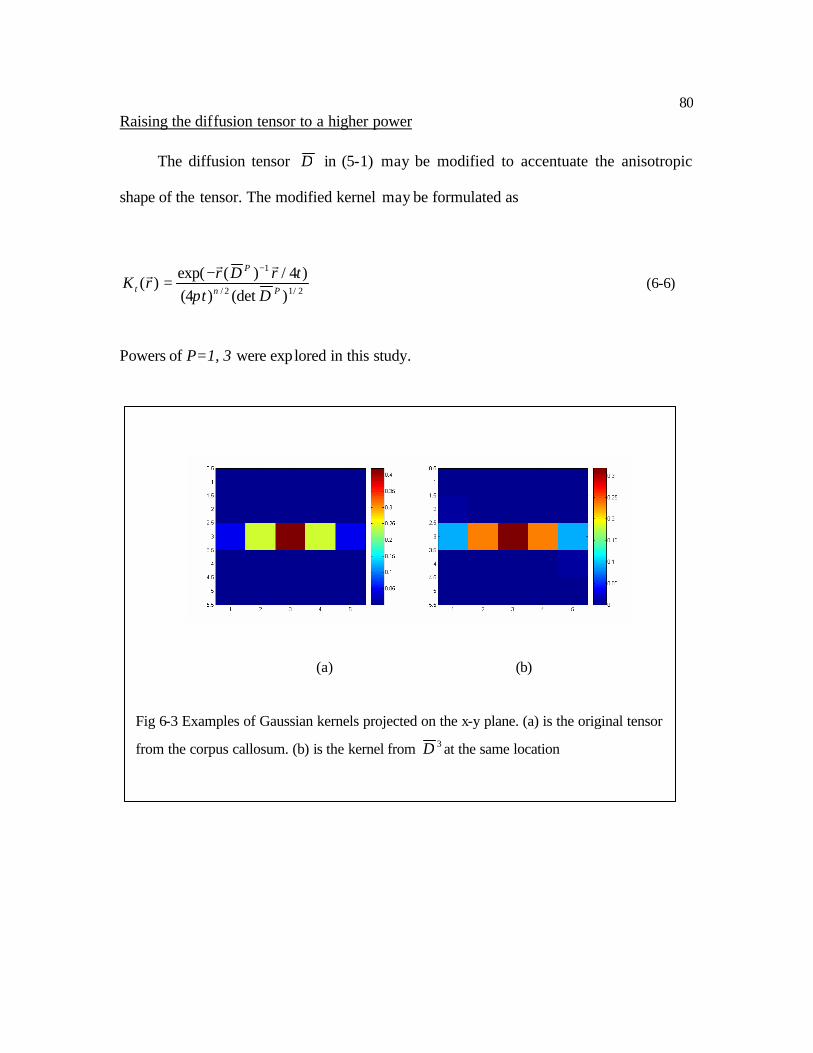
80 Raising the diffusion tensor to a higher power

The diffusion tensor D in (5-1) may be modified to accentuate the anisotropic

shape of the tensor. The modified kernel may be formulated as

2/12/

1

)(det)4()4/)(exp(

)(Pn

P

t DttrDr

rKπ

rrr −−

= (6-6)

Powers of P=1, 3 were explored in this study.

(a) (b)

Fig 6-3 Examples of Gaussian kernels projected on the x-y plane. (a) is the original tensor

from the corpus callosum. (b) is the kernel from 3D at the same location

81 Human brain data

The averaged (gold standard) DW data used in chapter 4 was employed in this

chapter to generate diffusion tensor and corresponding anisotropic Gaussian kernels. For

human brain data, a bigger widow (5 x 5 x 5 voxels) was used to facilitate regions of

curvature that are very commonly encountered in the brain data whereas the window that

was used for the previous simulation in the simplistic phantom was 3 x 3 x 3 voxels.

6.4 Results

Simulated phantom

Fig 6-4 was generated without using the conventional threshold to mask low

anisotropy regions. From the seeding point (in Fig 6-1), the diffusion profiles were

spreading out in the fiber directions and toward crossing regions, the diffusion became

separated into the three directions shown by the arrows.

The formulation of Fig 6-5-(a) to (c) is the same as for the Fig 6-4 except, in Fig 6-

5 all diffusion propagation was restricted in the region of FA>0.1. As shown in Fig 6-5

(d) to (e) compared against Fig 6-5 (a) to (c), raising the power of the tensor improved the

degree of anisotropy.

Human brain data

Fig 6-6 was generated using the power of P=1 (6-2). Increased power of the tensor

propagated faster, however, it did not change the overall propagation maps as noticeably

82 as in the simulation.

The starting seed point was placed at splenium (shown in Fig 6-6 a), and the

diffusion propagation was only allowed in the region of FA > 0.2. As the iteration of

convolution increased, the diffusion tended to propagate more in the direction of the

streamline tractography (Fig 6-6 f).

83

(a) (b) (c)

(d) (e) (f)

Fig 6-4. An example of the convolution smoothing with a seed point. (a), (b), and (c) are the

maps of sagittal, coronal, and axial view of a diffusion map at the level of iteration=40. (d), (e),

and (f) are from the iteration=200. Note that the diffusion propagation was not restricted in this

simulation, and restriction was allowed in Fig (6-5). The color is displayed in log scale (-log1/p)

of the diffusion probability, p

84

(a) (b) (c)

(d) (e) (f)

Fig 6-5 an example of effect of powers of the tensor. Increasing the power, p of PD increases the

propagation velocity with the same t value for 1D . Using a 3x3x3 window, with t value 0.05, (a),

(b) and (c) show sagittal, coronal, and axial views of using 1D and FA threshold mask (FA>0.1).

(d), (e), and (f) are sagittal, coronal, and axial view of using 3D . Gaussian convolution was

applied 200 times with a t value of 0.05. Raising the power p, ( PD ), can accentuate the

anisotropy shape of the tensor. Note that with the same t value and the same iteration of

performance, the 3D case diffused faster in the fiber directions (Fig 6-5 b and e) and diffusion

perpendicular to the fiber direction was more restricted in the magnified sagittal view (Fig 6-5 a

and d). The sagittal views (a, d) are zoomed up for the better visualization. The color is displayed

in log scale (-log1/p) of the diffusion probability, p.

85

(a) (b) (c)

(d) (e) (f)

Fig 6-6 iterations at 1 (a), 10 (b), 40 (c), 200 (d), and 400 (e). In (f), a seed was positioned at the

same location as for the convolution simulation, and then the Runge-Kutta interpolation method,

with a FA threshold of 0.2, and an angle threshold of 45 degree, was used to generate a single

track. The color in a-e is displayed in log scale (-log1/p) of the diffusion probability, p

86

6.5 Discussion

The connectivity probabilistic maps via anisotropic Gaussian kernel smoothing

produced a propagation distribution that was based upon the voxel-wise diffusion tensor

maps. Since the Gaussian kernel exists in three dimensions, the convolution process leads

to the blurring in the non-major eigenvector directions. This ultimately leads to apparent

connectivity in all arbitrary directions. To relate this issue, recently Morris et al proposed

a method of estimating the statistical significance of connection using random walk

simulation and PICo probabilistic tracking method [Morris et al., 2006]. In their method,

a null connection frequency was set up with non-restricted random walk probability map

and an experimental frequency was based on the connection map by PICo algorithm

[Parker et al, 2003a]. A statistical test was conducted on the two distributions to achieve

and estimate the significance of the experimental frequency connection map. Although

their method was adopted to minimize distance-related artifacts, one of the problems of

their method is that it is difficult to regularize the overall distribution concentration by the

Monte Carlo algorithm. To compensate for this effect, the distributions from anisotropic

and isotropic smoothing were computed in this study. Instead of using z statistics in

[Morris et al., 2006] to estimate the significance, a new concept of tensor distance by

measuring the similarity or dissimilarity between the tensors using Kullback-Leibler (KL)

divergence [Wang and Vemuri, 2005] can be utilized for the study of significance of

connection.

The KL divergence is defined [Kullback and Leibler, 1951]

87

xdxqxp

xpqpKLr

rr

r∫=

)()(

log)()||( (6-7)

where p(x) is the “true” probability distribution, and q(x) is the null probability

distribution. )||( qpKL measures a natural distance (difference) between these two

distinct probability distributions.

For the probabilistic connectivity by anisotropic smoothing, the KL distance can be

a measure of dissimilarity between probabilistic map from isotropic smoothing (q(x)) and

anisotropic smoothing (p(x)). In Fig 6-7, the KL distance was measured between 1D and

I (identity matrix for isotropic smoothing). Fig 6-7 shows a diffusion propagation map

obtained using the isotropic Gaussian kernel smoothing (a) and anisotropic Gaussian

kernel smoothing (b). Fig 6-7-c is the dissimilarity measure using the Eqn (6-7).

Interestingly in Fig 6-7-c the higher dissimilarity was observed in the vertical direction

anisotropy bar (shaded in blue) and the KL distance decreased rapidly in the horizontal

direction across the crossing region (shaded in violet). The difference between these

crossing two directions was more evident in the KL maps. The reason for this

dissimilarity originated from the two different FA values; FA of horizontal bar is

0.824494 and the FA of the vertical bar is 0.874281, so that ultimately the relative

anisotropy was directed toward the vertical bar leaving smaller values at the horizontal

bar.

Fig 6-8-d shows an example of the KL distance obtained in the corpus callosum.

The modified KL distance xdxqxp

xpxqxp

qpKLr

rr

rrr

∫=)()(

log)()()(

)||(' was attempted to create

88 more realistic connectivity patterns shown in Fig 6-9. Applications of KL distance need

to be developed for determining statistical significance.

(a) (b)

(c)

Fig 6-7 numerical simulation. (a) isotropic smoothing (b) anisotropic smoothing (c) KL distance

at iteration 200.

89

(a) (b)

(c) (d)

90 Fig 6-8 (a) Isotropic smoothing map (b) anisotropic smoothing map. (c) Subtraction map of the

isotropic smoothing from the anisotropic smoothing map. (d) KL distance. A seed at the same

position in the Fig 6-4 Splenium. The KL distance (dissimilarity between isotropic smoothing and

anisotropic smoothing) is shown using the rainbow color scale.

(a) (b)

Fig 6-9 Modified KL distance for a seed situated at the same position as in the Fig 6-4 in the

Splenium of the corpus callosum. The distance (dissimilarity between isotropic smoothing and

anisotropic smoothing) is shown in the rainbow color scale. (b) is thresholded map for KL values

longer than 0.3 in (a).

91

CHAPTER 7

CONLUSIONS AND FUTURE RESEARCH PLANS

This thesis investigates several novel methods based upon anisotropic diffusion-

weighting and image filtering. A summary of each chapter is as follows:

Chapter 3: anisotropic optimization of diffusion-weightings reduces the variances

of FA and MD measurements in the corpus callosum up to ~56 %. The method presented

in this chapter is a desirable approach when a region is homogeneous and the tensor

shape and orientations are predictable a priori; however, if the region of interest is mixed

with different orientations, it may lead to erroneous results for characterizing each

different tissue type.

Chapter 4: anisotropic Gaussian kernel smoothing is compared with isotropic

Gaussian smoothing and the Perona Malik algorithm. The evaluation is done with a

simulation using both synthetic noisy data and real human brain data. The performance of

three spatial filtering methods for reducing errors of FA, MD and major eigenvector

orientation demonstrates that an optimum level of filtering reduces the errors for all

measures. The optimum performances of both the isotropic and anisotropic Gaussian

filters are similar, yet the anisotropic filter is much less prone to over- filtering.

Chapter 5: an application of the anisotropic Gaussian kernel smoothing is shown

92 through a group analysis of autism data. The anisotropic Gaussian filter is constructed

for each individual subject at a voxel level considering spatial transformation that takes

place during data normalization. The anisotropic Gaussian kernel smoothing on white

matter segmented DT measurements data preserves the more peripheral white matter

structures and the consequent blurring occurs in the direction of white matter directions

on the white matter segmented DT measurements (FA, MD, and eigenvalues). The ROI

analysis in the corpus callosum is more consistent with results from anisotropically

smoothed data. In addition, anisotropic smoothing shows fewer morphological

differences through the binary mask analysis implying that anisotropic smoothing

confounds the group analysis of DT-MRI measures less frequently.

Chapter 6: the connectivity probabilistic maps via anisotropic Gaussian kernel

convolution produces a propagation distribution that is based upon the voxel-wise

diffusion tensor maps. The evaluation is done with a simple numerical phantom and

human brain data. The diffusion propagation in the phantom behaves as the tensor field

guides in the phantom. The diffusion propagation in the splenium of the corpus callosum

is also consistent with known anatomical connectivity.

As mentioned in Discussions of the last two chapters 5, and 6, more vigorous

studies are required and to complete the work in depth. Subjects below are the future

works that will be pursued.

The group analysis of DT-MRI data for autism using either anisotropic or isotropic

smoothing will be performed in more detail using a range of kernel sizes and examining

possible covariates such as age and behavioral measures.

93 Anisotropic Gaussian kernel smoothing for voxel-based group analysis still

requires more thorough validation. Experiments for evaluating the strengths and

weakness need to be performed. The validity of anisotropic kernel smoothing for random

field theory still needs to be examined more thoroughly.

For the anisotropic kernel smoothing, further algorithmic development is necessary

to minimize unlikely pathways to reduce the occurrence of false positive connections.

94

REFERENCES

[1] A.L. Alexander, K.M. Hasan, M. Lazar, J.S. Tsuruda, and D.L. Parker, “Analysis of

partial volume effects in diffusion-tensor MRI,” Magn. Reson. Med., vol. 45, pp. 770-

780, 2001.

[2] A.L. Alexander, J.E. Lee, M. Lazar, R.M. Boudos, M.B. DuBray, T.R. Oakes, J. Lu,

E.K. Jeong, E.D. Bigler, and J.E. Lainhart, “Diffusion Tensor Imaging of the Corpus

Callosum in Autism,” NeuroImage (in press), 2006

[3] D.C. Alexander, C. Pierpaoli, P.J. Basser and J.C Gee, “Spatial Transformations of

Diffusion Tensor Magnetic Resonance Images,” IEEE Transactions on Medical

Imaging, vol. 20 pp 1131-1139, 2001.

[4] A.W. Anderson, “Theoretical Analysis of the Effects of Noise on Diffusion Tensor

Imaging,” Magn. Reson. Med., vol.46, pp. 1174-1188, 2001.

[5] P.A. Armitage and M.E. Bastin, “Utilizing the Diffusion-to-Noise Ratio to Optimize

Magnetic Resonance Diffusion Tensor Acquisition Strategies for Improving

Measurements of Diffusion Anisotropy”, Magn. Reson. Med., vol.45, pp. 1056-1065,

2001.

[6] R. Bammer, “Basic principles of diffusion-weighted imaging,” European Journal of

Radiology, vol. 45, pp. 169-184, 2003.

[7] N. Barnea-Goraly, S. Eliez, M. Hedeus, V. Menon, C.D. White, M. Moseley, and A.L.

Reiss, “White matter tract alterations in fragile X syndrome: preliminary evidence

from diffusion tensor imaging,” Am. J. Med. Genet, Part. B 118B, pp. 81-88, 2003.

95 [8] P.G. Batchelor, D. L. G. Hill, D. Atkinson, and F. Calamanten, “Study of

Connectivity in the Brain Using the Full Diffusion Tensor from MRI,” IPMI Lecture

Notes in Computer Science, vol. 2082, pp. 121-133, 2001.

[9] P. J. Basser, J. Matiello, and D. Le Bihan, “Estimation of the effective self-diffusion

tensor from the NMR spin echo,” J. Magn. Reson. B vol. 103, pp. 247-254, 1994.

[10] P. J. Basser, and C. Pierpaoli, “Microstructural and Physiological Features of

Tissues Elucidated by Quantative-Diffusion-Tensor MRI,” J Magn Reson., vol. 111,

pp 209-219, 1996.

[11] P. J. Basser, S. Pajevic, C. Pierpaoli, J. Duda, A. Aldroubi, “In Vivo Tractography

Using DT-MRI Data,” Magn. Reson. Med., vol. 44, pp.625-632, 2000a.

[12] P.J. Basser and S. Pajevic, “Statistical Artifacts in Diffusion Tensor MRI (DT-MRI)

Caused by Background Noise,” Magn. Reson. Med., vol. 44, pp. 41-50, 2000b.

[13] C. Beaulieu, “The basis of anisotropic water diffusion in the nervous system – a

technical review,” NMR Biomed., vol. 15, pp. 435 – 455, 2002.

[14] J. Burns, D. Job, M. E. Bastin, H. Whalley, T. MacGillivray, E.C. Johnstone, and S.

M. Lawrie, “Structural disconnectivity in schizophrenia: a diffusion tensor magnetic

resonance imaging study,” Br. J. Psychiatry, vol. 182, pp. 439-443, 2003.

[15] A. Brun, H. Knutsson, H-J. Park, M. E. Shenton, and C-F. Westin, “Clustering Fiber

Traces Using Normalized Cuts,” LCNS, vol. 3216, pp. 368-375, 2004.

[16] P.T. Callaghan, “Principles of Nuclear Magnetic Resonance Microscopy,” Oxford

Science Publications, pp 25-91, 1991.

96 [17] J. S. W. Campbell, K. Siddiqi, V. V. Rymar, A.F. Sadikot and G. B. Pike, “Flow-

based fiber tracking with diffusion tensor and q-ball data: validation and comparison

to principal diffusion direction techniques,” NeuroImage, vol. 27. pp. 725-736, 2005.

[18] F. Catte, P-L. Lions, J-M. Morel, and T. Coll, “Image selective smoothing and edge

detection by nonlinear diffusion,” SIAM journal on Numerical Analysis vol. 29 (1),

pp. 182-193, 1992.

[19] M.K. Chung, M. Lazar, A. L. Alexander, Y. Lu, and R. Davidson, “Probabilistic

Connectivity Measure in Diffusion Tensor Imaging via Anisotropic Kernel

Smoothing,” UW Dept of Stats Technical Report NO. 1081, 2003.

[20] T. E. Conturo, N. F. Lori, T.S. Cull, E. Akbudak, A. Z. Snyder, and J.S. Shimony,

“Tracking neuronal fiber pathways in the living human brain,” Proceeding of the

National Academy of Sciences of the USA, vol. 96, pp. 10422-10427, 1999.

[21] O. Coulon, D.C. Alexander, and S. Arridge, “Diffusion tensor magnetic resonance

image regularization,” Medical image analysis, vol. 8, pp.47-67, 2004.

[22] Z. Ding, J.C. Gore, and A.W. Anderson, “Reduction of Noise in Diffusion Tensor

Images Using Anisotropic Smoothing,” Magn. Reson. Med., vol. 53, pp. 485-490,

2005.

[23] S. H., Erikkson, F. J. Rugg-Gunn, M.R. Symms, G. J. Barker, and J.S. Duncan,

“Diffusion tensor imaging in patients with epilepsy and malformations of cortical

development,” Brain, vol. 124, pp. 617-626, 2001.

[24] C. M. Filley, “White Matter and Behavioral Neurology. ” Ann. N.Y. Acad. Sci.

vol.1064, pp.162-183, 2005.

97 [25] C. D. Good, I. S. Johnsrude, J. Ashburner, R. N. A. Henson, K. J. Friston, and R.

S. J. Frackowiak, “A voxel-Based Morphometric Study of Ageing in 465 Normal

Adult Human Brains,” NeuroImage, vol. 14, pp.21-36, 2001.

[26] K.M. Hasan, D.L. Parker, and A.L. Alexander, “Comparison of Gradient Encoding

schemes for Diffusion-Tensor MRI,” JMRI., vol. 13, pp. 769-780, 2001a.

[27] K.M. Hasan, D.L. Parker, and A.L. Alexander, “Analytical Computation of the

Eigenvalues and Eigenvectors in DT-MRI”, J Magn Reson., vol. 152, pp. 41-47,

2001b.

[28] M. Jackowski, C. Y. Kao, M. Qiu, R. T. Constable, and L.H. Staib, “ White matter

tractography by anisotropic wavefront evolution and diffusion tensor imaging,”

Medical Image Analysis, vol. 9, pp. 427-440, 2005.

[29] P. Jezzard, and R.S. Balaban, “Correction for geometric distortion in echo planar

images from B0 field variations,” Magn. Reson. Med., vol. 34, pp. 65-73, 1995.

[30] D.K. Jones, M.A. Horsfield, and A. Simmons, “Optimal Strategies for Measuring

Diffusion in Anisotropic Systems by Magnetic Resonance Imaging,” Magn. Reson.

Med., vol. 42, pp. 515-525, 1999.

[31] D.K. Jones, A. Simmons, S.C.R. Williams, and M.A. Horsfield, “Non-Invasive

Assessment of Axonal Fiber Connectivity in the Human Brain Via Diffusion Tensor

MRI,” Magn. Reson. Med., vol. 42, pp. 37-41, 1999.

[32] D.K. Jones, L.D. Griffin, D.C. Alexander, M. Catani, M. A. Horsfield, R. Howard

and S. C. R. Williams, “Spatial Normalization and Averaging of Diffusion Tensor

MRI data Sets,” NeuroImage, vol. 17, pp. 592-617, 2002.

98 [33] D.K. Jones, “Determination and Visualizing Uncertainty in Estimates of Fiber

Orientation From Diffusion Tensor MRI,” Magn. Reson. Med., vol. 49, pp. 7-12,

2003.

[34] D.K. Jones, M.R. Symms, M. Cercignani and R. I. Howard, “The effects of filter

size on VBM analyses of DT-MRI data,” NeuroImage, vol. 26, pp. 546-554, 2005.

[35] M. Koch, V. Glauche, J. Finsterbusch, U. Nolte, J. Frahm, and C. Buchel,

“Estimation of anatomical connectivity from diffusion tensor data, “ NeuroImage, vol.

13, S176, 2001.

[36] M.A. Koch, D.G. Norris, and M. Hund-Georgiadis, “An investigation of functional

and anatomical connectivity using magnetic resonance imaging,” NeuroImage, vol.

16 pp. 241-250, 2002.

[37] J. Koenderink, “The Structure of Images,” Biological Cybernetics vol. 50, pp. 363-370,

1984.

[38] S. Kullback and R. A. Leible, “On information and sufficiency,” Annals of

Mathematical Statistics, vol. 20, pp. 79-86, 1951.

[39] M. Lazar, D.M. Weinstein J.S. Tsuruda, K.M. Hasan, K. Arfanakis, M.E. Meyerand,

B. Badie, H,A,Rowley, V. Haughton, A. Field, and A.L. Alexander, “White Matter

Tractography Using Diffusion Tensor Deflection,” Human Brain Mapping, vol. 18,

pp. 306-321, 2003a.

[40] M. Lazar, and A.L. Alexander, “An error analysis of white matter tractography

methods: synthetic diffusion tensor field simulations,” NeuroImage, vol. 20, pp.

1140-1153, 2003b.

99 [41] M. Lazar, and A.L. Alexander, “Bootstrap white matter tractography(BOOT-

TRAC),” NeuroImage, vol. 24, pp. 524-532, 2005.

[42] M. Lazar, A.L. Alexander, P.J. Thottakara, B. Badie, and A.S. Field, “White Matter

Reorganization after Surgical Resection of Brain Tumors and Vascular

Malformations,” AJNR Am J Neuroradiol, vol. 27, pp. 1258-71, 2006.

[43] D. Le Bihan, and P.J. Basser, “Diffusion and Perfusion Magnetic Resonance

Imaging,” Raven press, Chapter 1, 1995.

[44] D. Le Bihan, J.F. Mangin, C. Poupon, C.A. Clark, S. Pappata, N.Molko and H.

Chabriat, “ Diffusion Tensor Imaging: Concepts and Applications,” Journal of

Magnetic Resonance Imaging, vol. 13, pp. 534-546, 2001.

[45] J.E. Lee, and A.L. Alexander, “Optimized diffusion tensor encoding schemes with

anisotropic diffusion weighting,” 12th Annual ISMRM meeting, Kyoto, Japan, 2004.

[46] J.E. Lee, M .K Chung and A.L. Alexander, “Evaluation of Anisotropic Filters for

Diffusion Tensor Imaging,” 3rd IEEE International Symposium on Biomedical

Imaging: Macro to Nano, pp 77-80, 2006.

[47] L. H. Leung, G.C. Ooi, D.L. Kwong, G.C. Chan, G. Cao, and P.L. Khong, “White

matter diffusion anisotropy after chemo-irradiation: a statistical parametric mapping

study and histogram analysis,” NeuroImage, vol. 21, pp. 261-268, 2004.

[48] Z-P. Liang and P.C. Lauterbur, “Principles of Magnetic Resonance Imaging, A

Signal Processing Perspective,” IEEE Press Series in Biomedical Engineering, Wiley-

IEEE Press; 1st edition , 1999

[49] C.C. Lin, and L.A. Segel, “Mathematics Applied to Deterministic Problems in the

Natural Sciences”. 1988

100 [50] P. Mansfield, J. Physics, C10, L 55, 1977.

[51] J. Mattiello, P.J. Basser, and D. Le Bihan, “The b matrix in diffusion tensor echo-

planar imaging,” Magn. Reson. Med., vol. 37, pp. 292-300, 1997.

[52] S. Mori, B.J. Crain, V.P. Chacko, and P.C. Van Zijl, “Three-dimensional tracking of

axonal projections in the brain by magnetic resonance imaging,” Ann. Neurol., vol. 45,

pp. 265-269, 1999.

[53] D. M. Morris, K. V. Embleton, and G. J. Parker, “Definition of connection

significance using probabilistic tractography,” 14th Annual ISMRM meeting, Seattle,

WA, 2006.

[54] M. E. Moseley, “Diffusion tensor imaging and aging-A review,” NMR Biomed., vol.

15, pp. 553-560, 2002.

[55] J. Neil, P. Miller, P. S. Mukherjee, and P. S. Huppi, “Diffusion tensor imaging of

normal and injured developing human brain-A technical review,” NMR Biomed., vol.

15, pp. 543-552, 2002.

[56] D.G. Nishimura, “Principles of Magnetic Resonance Imaging,” Stanford University,

1996.

[57] L. O’Donnell, S. Haker, and C-F. Westin, “New Approaches to Estimation of White

Matter Connectivity in Diffusion Tensor MRI: Elliptic PDEs and Geodesics in a

Tensor-Warped Space,” LCNS, vol. 2488, pp. 459-466, 2002.

[58] S. Pajevic, A. Aldroubi, and P.J. Basser, “A continuous tensor field approximation

of discrete DT-MRI data for extracting Microstructural and architectural features of

tissues,” J Magn Reson., vol. 154, pp. 85-100, 2002.

101 [59] S. Pajevic, and C. Pierpaoli, “Color schemes to represent the orientation of

anisotropic tissues from diffusion tensor data: application to white matter fiber tract

mapping in the human brain,” Magn. Reson. Med., vol. 42, pp. 526-540, 1999.

[60] N.G. Papadakis, D. Xing, C. L. H. Huang, L. D. Hall, and T.A. Carpenter,

“Comparative study of acquisition schemes for diffusion tensor imaging using MRI,”

JMR., vol. 137, pp. 67-82, 1999.

[61] G.J.M. Parker, J.A. Schnabel, M.R. Symms, D.J. Werring, and G.J. Barker,

“Nonlinear Smoothing for Reduction of Systematic and Random Errors in Diffusion

Tensor Imaging,” JMRI., vol.11, pp. 702-710, 2000.

[62] G.J.M. Parker, C.A.M. Wheeler-Kingshott, and G.J. Barker, “Estimating Distributed

Anatomical Connectivity Using Fast Marching Methods and Diffusion Tensor

Imaging,” IEEE Trans on Medical Imaging vol. 21, pp. 505-512, 2002.

[63] G.J.M. Parker, H. A. Haroon, and C. A.M. Wheeler-Kingshott, “A Framework for a

Streamline-Based Probabilistic Index of Connectivity (PICo) Using a Structural

Interpretation of MRI Diffusion Measurements,” JMRI, vol. 18, pp. 242-254, 2003a.

[64] G. J. M. Parker and D. C. Alexander, “Probabilistic Monte Carlo based mapping of

cerebral connections utilizing whole-brain crossing fiber information,” Lecture Notes

in Computer Science, vol. 2737, pp. 684-695, 2003b.

[65] P. Perona, and J. Malik, “Scale-space and edge detection using anisotropic

diffusion,” IEEE Trans. Pattern Anal. Machine Intell, vol.12, pp. 629–639, 1990.

[66] C. Pierpaoli, and P.J. Basser, “Toward a quantitative assessment of diffusion

anisotropy,” Magn. Reson. Med., vol. 36, pp. 893-906, 1996.

102 [67] M.A. Rodriguez-Florido, C-F. Westin, and J. Ruiz-Alzola, “DT-MRI

regularization using anisotropic tensor field filtering,” In: 2004 IEEE International

Symposium on Biomedical Imaging - April 15-18 - Arlington, VA (USA). pp. 336–

339.

[68] A. Rosenfeld, and A.C. Kak, “Digital Picture Processing 2.” Academic Press,

Orlando, FL, p.42, 1982.

[69] L. A. Segel, Mathematics Applied To Continuum Mechanics, 1977.

[70] R.I. Shrager, and P.J. Basser, “Anisotropically weighted MRI,” Magn. Reson. Med.,

vol. 40, pp. 160-165, 1998.

[71] M. Sommer, M.A. Koch, W. Paulus, C. Weiller, and C. Buchel, “Disconnection of

speech-relevant areas in persistent developmental stuttering, ” Lancet, vol. 360,

pp.380-383, 2002.

[72] C. H. Sotak, “The role of diffusion tensor imaging in the evaluation of ischemic

brain injury-A review,” NMR Biomed., vol. 15, pp. 561-569, 2002.

[73] J-D, Tournier, F. Calamante, D.G . Gardian, and A. Connelly, “Diffusion –weighted

magnetic resonance imaging fiber tacking using a front evolution algorithm,”

NeuroImage, vol. 20, pp. 276-288, 2003.

[74] D. Tschumperle, and R. Deriche, “DT-MRI: Estimation, Regularization and

Applications,” Eurocast 2003, 9th international conference on computer aided

systems theory.

[75] M.T. Vlaardingerborek and J.A. den Boer, “Magnetic Resonance Imaging” second

edition, Springer.

103 [76] Z. Wang, B.C. Vemuri, Y. Chen, and T.H. Mareci, “A Constrained Variational

for Direct Estimation and Smoothing of the Diffusion Tensor Field From complex

DWI,” IEEE Transactions on medical imaging, vol. 23, pp. 930-939, 2004.

[77] Z. Wang, B.C. Vemuri, Y. Chen Y, T. Mareci, “Simultaneous Smoothing and

Estimation of the Tensor Field from Diffusion Tensor MRI,” CVPR. 2003.

[78] Z. Wang, and B.C. Vemuri, “DTI Segmentation Using an Information Theoretic

Tensor Dissimilarity Measure,” IEEE Transactions on medical imaging, vol. 24, pp.

1267-1277, 2005.

[79] J. Weickert, “Coherence-enhancing diffusion of colour images,” Image and Vision

Computing, vol. 17, pp. 201-212, 1999.

[80] D. Weinstein, G. Kindlmann, and E. Lundberg, “Tensorlines: Advection-Diffusion

based Propagation through Diffusion Tensor Fields,” IEEE Visualization Proceedings

of the conference on Visualization ’99: celebrating ten years, pp. 249-253, 1999.

[81] William H. Press Numerical recipes in C: The art of scientific computing

[82] K. J. Worsley, A. C. Evans, S. Marrett, and P. Neelin, “A three dimensional

statistical analysis for CBF activation studies in human brain,” J. Cereb. Blood Flow

Metab., vol. 12, pp. 900-918, 1992.

[83] D. Xing, N.G. Papadakis, C. L. -H. Huang, M. L. Vee, T. A. Carpenter and L. D.

Hall, “Optimised diffusion-weighting for measurement of apparent diffusion

coefficient (ADC) in human brain,” Magnetic Resonance Imaging, vol. 15, pp. 771-

784, 1997.

104 [84] J. Zhang, N. Kang, and S. E. Rose, “Approximating Anatomical Brain

Connectivity with Diffusion Tensor MRI Using Kernel-Based Diffusion

Simulations,” LNCS, vol. 3565, pp. 64-75, 2005.

[85] Y. Zhang, M. Brady, and S. Smith, “Segmentation of Brain MR Images through a

Hidden Markov Random Field Model and the Expectation-Maximization Algorithm,”

IEEE Transactions on Medical Imaging, vol. 20, pp. 45-57, 2001.

105 Appendix A

Diffusion equation from Brownian motion

Consider the one dimensional case, a particle moves between ∆ and ∆+∆ d in a

time intervalτ with probability ∆∆φ d)( , the probability distribution must satisfy

∫+∞

∞−

=∆∆ 1)(φd , (A-1)

)()( ∆−=∆ φφ , (A-2)

0)( →∆φ as ∞→∆ || , (A-3)

If )t,x(C is the density of the particles at time t , the total number of particles

∫+∞

∞−

= dx)t,x(CN (A-4)

At time τ+t , the density is ∆∆∆φτ d)t,x(C)()t,x(C ∫+∞

∞−

−=+ (A-5)

Using the Taylor expansion

L++=+dtdC

)t,x(C)t,x(C ττ

L+∂∂

+∂∂

−=−2

22

xC

2xC

)t,x(C)t,x(C∆

∆∆

106 Substituting Taylor terms into (A-5)

∫∫∫∞

∞−

∞

∞−

∞

∞− ∂∂

+∂∂

−=∂∂

+ ∆∆

∆φ∆∆∆φ∆∆φτ d2

)(xC

d)(xC

d)(CxC

C2

2

2

(A-6)

Using the property of (A-1) and (A-2), (A-6) leads to 2

2

xC

DtC

∂∂

=∂∂

107 Appendix B

Diffusion equation from Random walk

Let ),( Nmw be the probability that a particle will arrive m steps to the right after

taking a total of N steps, and then (B-1) should be satisfied. This is called the difference

equation.

),(21

),(21

),( txxwtxxwttxw ∆++∆−=∆+ (B-1)

),(),(t

tx

xwtxw

∆∆≡ (B-2)

Thus )t,x(w is the probability that the particle which starts at the origin at time t=0

is located at point at time t.

),x(mx ∆= ),t(Nt ∆= (B-3)

Since we are interested in the solution only after the particle has taken a large

number of steps

0t,N →∞→ ∆ 0x,m →∞→ ∆ (B-4)

expanding the functions in (B-1) by the Taylor’s expansion

322 )())(,(21

)(),( xOxtxwtOttxw xxt ∆+∆=∆+∆ (B-5)

108

Dividing each term by t∆2 and setting (B-6), the diffusion equation (B-7) is derived.

,2

)( 2

0,0lim D

tx

tt=

∆∆

→∆→∆ ,0≠D (B-6)

xxt wDw = (B-7)

109 Appendix C

Derivation of the covariance of directional diffusitivities

)(12 ∑=

N

kj

ki

kjDD DD

Ni δδσ

)()(1

00

00

jk

j

jk

kjk

ik

i

ikN

k

kik

SS

DS

S

DS

SD

SSD

Nδδδδ

∂

∂+

∂

∂×

∂∂

+∂∂

= ∑

Since ji0 S,S,S are all independent of each other their cross multiplication is zero

)(1 2

000

SS

D

SD

Nkj

kN

k

ik

δ∂

∂

∂∂

= ∑

02

00

11S

ji SbSbσ=

02

20

1S

ji Sbbσ= (C-1)

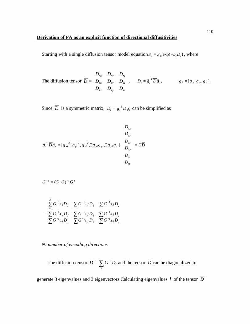
110 Derivation of FA as an explicit function of directional diffusitivities

Starting with a single diffusion tensor model equation )exp(0 iii DbSS −= , where

The diffusion tensor ,DDDDDDDDD

D

zzzyzx

yzyyyx

xzxyxx

= iT

ii gDgDrr

= , izyxi gggg ],,[=

Since D is a symmetric matrix, iT

ii gDgDrr

= can be simplified as

DG

DD

DD

DD

ggggggggDg

yz

xz

xy

zz

yy

xx

ziyiyixiziyixiiT

i =

⋅= ]2,2,,,[ 222rr

TT GGGG 11 )( −− =

=

∑∑∑∑∑∑

∑∑∑

−−−

−−−

−−

=

−

jjjjjj

jjjjjj

jjjj

N

jjj

DGDGDGDGDGDG

DGDGDG

,31

,61

,51

,61

,21

,41

,51

,41

1,1

1

N: number of encoding directions

∴ The diffusion tensor ∑ −=i

i1DGD and the tensor D can be diagonalized to

generate 3 eigenvalues and 3 eigenvectors Calculating eigenvalues λ of the tensor D

111

0DGDGDG

DGDGDG

DGDGDG

jj,31

jj,61

jj,51

jj,61

jj,21

jj,41

jj,51

jj,41

N

1jjj,1

1

=−

−

−

∑∑∑∑∑∑∑∑∑

−−−

−−−

−−

=

−

λλ

λ

(C-2)

Solving the (C-2), iλ becomes a function of iD , which makes FA to be an explicit

function of iD using invariants.

)(

)()()(23

23

22

21

32

22

1

λλλ

λλλλλλ

++

><−+><−+><−= iiiFA (C-3)

Another approach to find the FA as an explicit function of iD would be using the

invariants of the tensor and numerical methods. The invariants are as follows:

The numerical approach of finding eigenvalues is

zzyyxx DDDI ++=1

)( 2222 xzyzxyxxzzzzyyyyxx DDDDDDDDDI ++−++=

)(2 2223 xzyyyzxxxyzzyzxzxyzzyyxx DDDDDDDDDDDDI ++−+= (C-4)

3/)/1/cos(

2/6/)3/(

3/)3/(

3213

1

22

1

vvsa

IIIIs

IIv

×=

+−=

−=

φ

)3/cos(23/

)3/cos(23/

)cos(23/

13

12

11

φφλ

φφλ

φλ

−××−=

+××−=

××+=

vI

vI

vI

(C-5)

112

By inserting the (C-5) into (C-3) , )I2I(

I1FA

22

1

2

−−= , which leads to the FA is an

explicit function of diffusitivities iD

113 Appendix D

Positive Definite

A positive definite tensor is not altered throughout the kernel convolution as long

as all tensor elements within the discrete integral window are positive definite. If the

weighting factor is ijk njni ,,1,,,1 LL == window size= nxn

1=∑ ijk

Assuming the tensor

=

zzzyzx

yzyyyx

xzxyxx

DDDDDDDDD

T is positive definite then, for any vector, ),,( zyxr =r ,

0' >rTrrr

0222222 >+++++ xzyzxyzzyyxx xzDyzDxyDDzDyDx

the new tensor after kernel convolution, T’ may expressed as following

ijxxD means that xxD values in the ji, position.

=

∑∑∑∑∑∑∑∑∑

ijzzij

ijzyij

ijzxij

ijyzij

ijyyij

ijyxij

ijxzij

ijxyij

ijxxij

DkDkDk

DkDkDkDkDkDk

T '

calculating '' rTr rr

ijxzij

ijyzij

ijxyij

ijzzij

ijyyij

ijxxij DkxzDkyzDkxyDkzDkyDkx ∑∑∑∑∑∑ +++++ 222222

114

)222( 222 ijxz

ijyz

ijxy

ijzz

ijyy

ijxxij xzDyzDxyDDzDyDxk +++++= ∑

let ijxz

ijyz

ijxy

ijzz

ijyy

ijxxij xzDyzDxyDDzDyDxA 222222 +++++=

if all tensors in j,i position are positive definite, then 0Aij >

∑ >= 0ijij Ak

Applying the kernel to the directional diffusitivity is the same as the applying the

kernel to the tensor due to the linearity

ii TggD ',=

GTD =

DGGGT ')'( 1−= ')'( 1GGG − is a constant matrix.

∴ T is proportional to D

anisotropic acquisition and analysis for diffusion tensor...

Documents