Animal Breeder's Tool KitUser's Guide and Reference Manual

B. L. Golden, W. M. Snelling and C. H. Mallinckrodt1

1 Assistant professor, research associate and graduate assistant, Department of AnimalSciences.

The authors wish to thank Dr. Richard Bourdon, Associate Professor, Department ofAnimal Sciences, Dr. James Brinks, Professor, Department of Animal Sciences, and Dr.Thomas Field, Assistant Professor, Department of Animal Sciences for their commentsand assistance in the preparation of this bulletin.

These manuals describe release 1 of the abtk software.

Animal Breeder's Tool Kit

User's Guide

User's Guide Table of Contents

1 User Environment, Terminology and Definitions . . . . . . . G-1About This Document . . . . . . . . . . . . . . . . . . . . . . . . . . . . . . . . . . . . . G-2The User Environment . . . . . . . . . . . . . . . . . . . . . . . . . . . . . . . . . . . . . G-3Definitions and Terminology . . . . . . . . . . . . . . . . . . . . . . . . . . . . . . . . G-5Adding New Routines . . . . . . . . . . . . . . . . . . . . . . . . . . . . . . . . . . . . . G-5Obtaining a Copy of abtk . . . . . . . . . . . . . . . . . . . . . . . . . . . . . . . . . . . G-6

2 Preparing Data for Analysis . . . . . . . . . . . . . . . . . . . . . . . . G-7The Unix User Utilities . . . . . . . . . . . . . . . . . . . . . . . . . . . . . . . . . . . . G-7Missing Values . . . . . . . . . . . . . . . . . . . . . . . . . . . . . . . . . . . . . . . . . . . G-8

3 Storage Modes . . . . . . . . . . . . . . . . . . . . . . . . . . . . . . . . . . . G-10General Description of Storage Modes . . . . . . . . . . . . . . . . . . . . . . . G-10

4 Basic Commands for Assembling Linear Systems . . . . . G-13An Example Model . . . . . . . . . . . . . . . . . . . . . . . . . . . . . . . . . . . . . . G-13Equation for the Mean . . . . . . . . . . . . . . . . . . . . . . . . . . . . . . . . . . . . G-14Incidence of the Fixed Effects . . . . . . . . . . . . . . . . . . . . . . . . . . . . . . G-15Concatenating the Blocks . . . . . . . . . . . . . . . . . . . . . . . . . . . . . . . . . . G-16Creating the Normal Equations. . . . . . . . . . . . . . . . . . . . . . . . . . . . . . G-17

5 Assembling Single Trait Animal Models . . . . . . . . . . . . . G-18Constructing the Inverse NumeratorRelationship Matrix . . . . . . . . . . . . . . . . . . . . . . . . . . . . . . . . . . . . . . G-19Assembling the Normal Equations . . . . . . . . . . . . . . . . . . . . . . . . . . G-20Maternal Effects Model . . . . . . . . . . . . . . . . . . . . . . . . . . . . . . . . . . . G-21Maternal Effects Normal Equations . . . . . . . . . . . . . . . . . . . . . . . . . . G-23

6 Assembling Reduced Animal Models . . . . . . . . . . . . . . . . G-25Forming the Normal Equations . . . . . . . . . . . . . . . . . . . . . . . . . . . . . G-27

7 Assembling Multiple Trait Models . . . . . . . . . . . . . . . . . . G-28Multiple Trait Normal Equations . . . . . . . . . . . . . . . . . . . . . . . . . . . . G-28Inverse Residual Matrix Blocks . . . . . . . . . . . . . . . . . . . . . . . . . . . . . G-29RAM Multiple Trait Models . . . . . . . . . . . . . . . . . . . . . . . . . . . . . . . G-29

8 Solving The Linear System . . . . . . . . . . . . . . . . . . . . . . . . G-31Direct Solution Using an Inverse . . . . . . . . . . . . . . . . . . . . . . . . . . . . G-31Iterative Solution . . . . . . . . . . . . . . . . . . . . . . . . . . . . . . . . . . . . . . . . G-31

G-1

1 User Environment, Terminologyand Definitions

The Animal Breeder's Tool Kit (abtk) is a software package that assists thetechnically trained animal breeder in assembling and solving equation systems withoutneeding to know a third generation programming language such as FORTRAN or C.The abtk was originally developed around the linear systems common in animal breedingproblems. However, it was intended to be flexible enough that it should accommodatea wide variety of equation systems, linear or otherwise. Obviously, the field ofmathematics is such that not all routines to construct and solve every possible equationsystem are incorporated in this package. But the current release of abtk includes asubstantial number of tools that will assist most all users working in the field of livestockgenetics and form a foundation that can be built upon. It is hoped and intended that ifroutines a particular user finds helpful to fulfill his particular research needs are missing,he will develop them and share them with the rest of the animal breeding community bymaking them available on the anonymous ftp site at Colorado State University. Theprocedure for doing this is discussed later in this chapter.

We are certain that to try and accomplish for mixed models what, say, SAS(1990) PROC GLM has done for fixed models would be impossible. It may be possibleto prepare some subset of useful models, but even specifying the structure and solutioncharacteristics of the most basic mixed models is much more complex then fixed effectsanalysis. Thus, we have chosen the "toolkit" approach.

To some more experienced users part of the abtk will look and behave like theolder symbolic matrix interpreters such as SMIS or SAS's PROC MATRIX. Becausewe are targeting this package at trained animal breeders it was important to be able totake the information from literature and easily transfer it to application. Therefore,many parts of the system look like symbolic matrix interpretation. However, asexplained in detail in the Technical Reference, the underlying algorithms and datastorage modes are very dissimilar from traditional matrix packages. Traditionalapproaches to software for matrix interpretation have been limited in size of equationsystems due to algorithm performance and data storage modes. For the most part thealgorithms used in the abtk avoid these limitations.

The abtk was designed to take advantage of what appear to be the most promisingtrends in performance computing. The advent of small (in physical size), highperformance architectures with large memory and high speed I/O devices has directedthe development of the methods used in the abtk. Because of the success in thedevelopment of technology such as RISC computing, the algorithms are based on highspeed scaler processing with I/O that uses large band widths. The methods used in theabtk were not explicitly coded for a particular hardware configuration and have beenused in environments ranging from UNIX running on an Intel 80386 processor at 25 Mhto a Cray Y/MP 864. All algorithms take advantage of dynamic memory allocation and,thus problem size is limited only by the available memory and mass storage capacity ofthe system.

About This Document

G-2

The documentation for the abtk consists of three manuals. The first manual is a"Users Guide." This guide is not meant to be a training manual in best linear unbiasedprediction, but it does demonstrate how to build several mixed model linear systemsusing the abtk. It is hoped users will find this document a useful reference manual fornot only the software but also common methods and notations used by animal breeders.Many users should find the appendix particularly helpful.

The discussion of the abtk in the guide is strictly limited to its use in linearmodels. Once a substantial number of routines have been developed for handling othertypes of linear or non-linear systems a supplementary guide will be developed.However, even though only fixed and mixed model systems common in animal breedingare discussed, abtk is not limited to these uses.

The second manual is the "Reference Manual." The reference manual is analphabetized list of the commands and their descriptions. Users are strongly encouragedto keep a copy of the reference manual available when working with the abtk. Theprinted paper copy of the Reference Manual and the Users Guide are bound together.

A good UNIX reference is also necessary. The abtk is closely bound to the UNIXoperating system and many of the data manipulations that users make are performedusing the UNIX user utilities (awk, join, sort, etc.). For a discussion of the UNIX userutilities any good UNIX reference and guide will work. Many other public domain orfreeware utilities exist for UNIX. Users may want to supplement the user utilities witha package such as Perl, an advanced data manipulation package that combines many ofthe features of awk, sed join and other UNIX utilities. Perl can be obtained from theusenet archives on the Internet. The discussion in this guide will be restricted to utilitiesthat are available on all UNIX systems.

The third manual, or "Technical Reference", is a discussion of the algorithms andstorage modes used by the abtk. This manual should be very useful for the applicationdeveloper who needs examples and ideas for expanding the abtk.

The User Environment

The abtk is closely bound to the UNIX user utilities. Early in the developmentof the abtk we realized that any animal breeder doing even the most basic statisticalanalysis would benefit from knowing the UNIX user utilities. Moreover, relying on theUNIX user utilities avoids the development of redundant routines and algorithms.

The abtk is a series of commands that process data into symbolic representationsof matrices and matrix components and solve the equation systems assembled. Thecommands are all given from the UNIX prompt (any shell). All commands generallyfollow the proposed ANSI specification for parameters and arguments, with oneexception for a few simple commands. This exception involves the order dependenceof arguments. For example, to multiply two matrices together and save them as a thirdmatrix the syntax would be,

mult A B C

G-3

indicating that matrix A is to be multiplied by matrix B and store in matrix C (where Apremultiplies B). The proposed standard for command arguments specifies argumentsshould be order independent, but this did not make sense for certain commands thatinvolved matrix operations. Most other commands use UNIX parameter flags indicatingwhat the argument is, and thus the arguments are order independent. For example, toiteratively solve a linear system, the following command could be used,

itgen -R beta.old -n coef -r rhs -m 1000 -b beta.new

This command would result in the iterative solution (Gauss-Siedel) using the vectorbeta.old for starting values, coef as the coefficient matrix, rhs as the right hand sidevector, 1000 as the maximum number of rounds to iterate and place the solutions intobeta.new. The arguments could be given in any order (just like a UNIX command).

In addition to using a UNIX like command syntax, the commands behave in aUNIX like fashion. If a command is issued without arguments it returns a syntaxmessage. This is particularly useful if the exact syntax of the arguments is forgotten.For example, if you have forgotten the syntax of the generalized incidence matrixconstruction routine, entering,

gen_z

will result in the following syntax explaination,

gen_z: Syntax: gen_z -d data_vector -e effect_list -r rhs_vector -o output_matrix

The abtk relies on the UNIX system to supply components that are critical to itsoperation. Several of the UNIX user utilities provide important data handlingcapabilities that must be performed in the setup of a problem for solution. The mostused commands are the awk pattern scanning and recognition language, the joinrelational data operator, the sort data sorter, and occasionally the paste horizontal flatfile concatinator.

The most often used user utility is awk. Awk is a very easy to use language thatgives you powerful data manipulation capability without needing to know a thirdgeneration programming language. For a complete and easily understood discussion ofthe awk language see "AWK Programming Language" (Aho, 1988) or any basic UNIXguide.

It is also useful for the advanced user to learn shell programming. The codes thatmake up the abtk are a mixture of C language, awk and bourne shell scripts. The abtkis intended to work like a macro language that is processed by the command interpreter.Users should not hesitate to program analyses they will use multiple times into a scriptprogram that they can batch process. The developers have had success taking thisapproach when performing even REML type analyses. Example scripts are includedwith the release version in the examples subdirectory.

Definitions and Terminology

G-4

The discussion in this manual is a blend of terms commonly used among UNIXusers and among animal breeders. Since this manual cannot instruct in every aspect ofcomputing or animal breeding, a certain level of understanding will be assumed. Thisdocumentation and the level of sophistication of the abtk is intended for people who havereceived or are currently enrolled in at least one graduate level course in mixed modelsmethodology.

A complete discussion of how the abtk forms and stores its matrices appears insection 3 of the Users Guide. It is important that the user understand how the UNIX filesystem works and particularly how it works with the abtk. The abtk uses an objectoriented approach. Each matrix and data vector must be thought of as an individualobject. It is helpful if the beginning user tries to forget his understanding of data files,file systems and data analysis developed from working in environments such as SAS,MS-DOS or LSML76. In the abtk each data vector from a traditional flat text file willbe stored in its own UNIX "file". Each matrix formed from data vectors or othermatrices will also be stored in a UNIX "file".

The user should take a structured approach to solving his particular problem. Forexample, the first step when assembling a particular problem is to separate a traditionalflat data file into separate data vectors for each column in the flat file. By storing eachdata vector of the flat file in a separate UNIX file, each vector can be worked with as aunique object. This is analogous to a typical fourth generation data base manager whereeach category is given a unique name, and the UNIX subdirectory where the flat file isstored can be thought of as the data table. Users can easily accomplish these types ofmanipulations using the UNIX user utilities. This guide contains many examples ofthese tasks.

Adding New Routines

The abtk can be useful for testing and developing new models or new algorithms.It is intended that as new research is performed, the abtk can provide a starting point, orat least an environment that will allow the researcher to develop new methods withouthaving to generate computer code that performs the setup work. For example, if aresearcher were working in solution methods for non-linear systems, abtk could providemany of the assembly routines for the equation systems. The researcher would then befree to concentrate on the solution algorithm.

Researchers who would like to use the abtk for this purpose are encouraged tostudy the abtk Technical Reference for a discussion of algorithms and storage modes.Pay particular attention to the way in which storage modes have increased not onlyproblem size but also performance of the operation. For an example, see the discussionof how the matrix multiply is performed with the SPARSE storage mode.

Obtaining a Copy of abtk

Users can obtain a magnetic copy free of charge from anonymous FTP atanonymous@cgel.agsci.colostate.edu. The abtk is distributed in a compressed tar fileso the user will need both an uncompress utility and a good tar (Unix tape archive)

G-5

utility. Both are made available through the Internet at several anonymous FTP sitesoffering the GNU software collection.

The distribution file contains magnetic copies of the manuals in post scriptformat. Users can also obtain copies of the manuals in WordPerfect format from theanonymous server.

Paper copies of the documentation can be obtained by contacting the Departmentof Animal Sciences, Colorado State University, Ft Collins, CO 80523. There will be acharge for the paper copies of the documentation to cover printing costs.

The abtk will also be distributed for a minimal $20 processing fee on reel-to-reeltape (6250 or 1600 bpi) in a compressed tar format.

Users with special needs are encouraged to contact the author to makearrangements.

G-6

2 Preparing Data forAnalysis

Data preparation for an abtk analysis is performed primarily using the UNIX userutilities. It is not recommended that a user attempt to supplement the data preparationtasks with a fourth generation relational database manager such as SAS or Oracle. Theexperiences of our shop indicate that it is more efficient to manage data using the UNIXuser utilities.

The objective is to prepare a data set to work the way animal breeders are trainedto think and to work the way information about models is presented in the literature.Therefore, the data must be organized according to the object oriented model. For alltraditional statistical analysis packages the data are managed as a flat file. In some ofthe more sophisticated commercial statistical software packages the data are managedusing an object oriented approach, but are managed as binary data held in a single filethat is not generally available to the researcher except through the data managementpackage. The abtk uses the data stored as text files (ASCII) and any component of thefiles are generally available to the user through the UNIX user utilities.

The Unix User Utilities

Typically, data analyzed in animal breeding studies are organized in one or aseries of two dimensional data files. The data structure in these data files is usuallyconceptualized as having categories represented as columns and items represented withdifferent rows. For example, take the following data file,

A 1 5 500B 2 3 450C 1 2 475D 1 5 550E 2 4 425F 2 5 490

Say this file represents six beef cattle weaning weight observations . The animalidentification is held in the first field (column). The second field is the sex code, 1=bulland 2=heifer. The third field represents the age in years of the dam, and the last fieldrepresents the observed weaning weight of each animal in a row (item).

Traditionally, these data would be held in a single file as input to the analyticalsoftware that would perform, say, a fixed model analysis of weaning weight. The abtkrequires that each field be held in a separate UNIX file. To the first time user thisapproach may seem a little awkward, but, with some experience users will realize thatthis is not different from traditional approaches except that now there is much moreprecise control of the contents of these files. They can be conceptualized as the objectsrepresented by notations commonly seen in animal breeding literature.

File names should correspond to the field contained in the file (id, sex, aod etc.).The name of the directory containing a series of files should reflect the contents of thedirectory. Working from our example data set above, say the file was copied into the

G-7

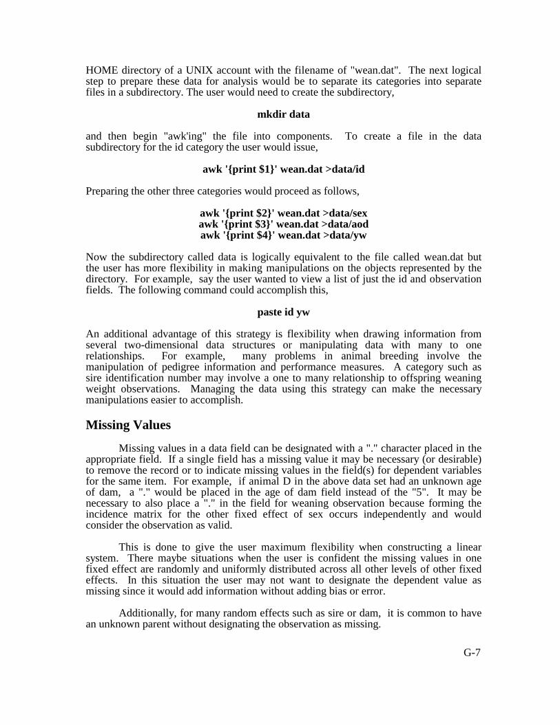
HOME directory of a UNIX account with the filename of "wean.dat". The next logicalstep to prepare these data for analysis would be to separate its categories into separatefiles in a subdirectory. The user would need to create the subdirectory,

mkdir data

and then begin "awk'ing" the file into components. To create a file in the datasubdirectory for the id category the user would issue,

awk '{print $1}' wean.dat >data/id

Preparing the other three categories would proceed as follows,

awk '{print $2}' wean.dat >data/sexawk '{print $3}' wean.dat >data/aodawk '{print $4}' wean.dat >data/yw

Now the subdirectory called data is logically equivalent to the file called wean.dat butthe user has more flexibility in making manipulations on the objects represented by thedirectory. For example, say the user wanted to view a list of just the id and observationfields. The following command could accomplish this,

paste id yw

An additional advantage of this strategy is flexibility when drawing information fromseveral two-dimensional data structures or manipulating data with many to onerelationships. For example, many problems in animal breeding involve themanipulation of pedigree information and performance measures. A category such assire identification number may involve a one to many relationship to offspring weaningweight observations. Managing the data using this strategy can make the necessarymanipulations easier to accomplish.

Missing Values

Missing values in a data field can be designated with a "." character placed in theappropriate field. If a single field has a missing value it may be necessary (or desirable)to remove the record or to indicate missing values in the field(s) for dependent variablesfor the same item. For example, if animal D in the above data set had an unknown ageof dam, a "." would be placed in the age of dam field instead of the "5". It may benecessary to also place a "." in the field for weaning observation because forming theincidence matrix for the other fixed effect of sex occurs independently and wouldconsider the observation as valid.

This is done to give the user maximum flexibility when constructing a linearsystem. There maybe situations when the user is confident the missing values in onefixed effect are randomly and uniformly distributed across all other levels of other fixedeffects. In this situation the user may not want to designate the dependent value asmissing since it would add information without adding bias or error.

Additionally, for many random effects such as sire or dam, it is common to havean unknown parent without designating the observation as missing.

G-8

G-9

3 Storage ModesSince it was intended in the design of this package to maximize performance

while optimizing utility, it was necessary to store and work with data held on massstorage in multiple storage modes. It is helpful (but probably not necessary) to have alimited understanding of the most common storage modes to effectively operate the abtk.The storage modes are the key to the feasibility of solving problems of realistic size.The storage modes help to increase the capacity of the software to handle large problemsby reducing wasted mass storage space and by allowing the implementation of specialalgorithms that take advantage of the features of some storage modes.

Users who want to develop additional tools are encouraged to carefully study thediscussion of storage modes in the technical reference.

General Description of Storage Modes

There are ten storage modes supported in the abtk. Not all ten are implementedin all routines, and thus for a few "non-typical" operations, translation of storage modesmay be necessary. For example, the routine ident, used to form an identity matrix,builds the identity matrix using only a storage mode called DIAGONAL.

Many routines accommodate several storage modes. The storage modes chosento be used by a given routine were determined by how likely it was that the routinewould receive as input a matrix in a given storage mode and what the effects of a givenstorage mode would be on the computer performance of the operation.

Users are encouraged to contact the developers and request changes in howstorage modes are implemented. If a given routine does not support a given storagemode, and the user sees this as a shortcoming, please contact the developers.

Headers, Text and Compression. All storage modes of data use a header recordexcept the storage mode called DEFAULT. The DEFAULT storage mode is atraditional storage method where a matrix or vector is stored as a complete, two-dimensional representation of the data. For example, when the example data set insection 1 of the Users Guide was separated into its component fields, each field wasstored in the DEFAULT storage mode. Another example is the following twodimensional matrix,

10 2020 30

If the user issued the UNIX cat command to a file that contained this matrix and itappeared as it does above, then the storage mode was DEFAULT.

All other storage modes have a header record. The header record is the first lineof the file. If a user uses the cat command to view the above matrix, and it was in, forexample, the SPARSE storage mode, it would appear as,

SPARSE 2 2 41 1 10

G-10

1 2 202 1 202 2 30

The first line of this five line file is the header record. The header record alwayscontains four fields. The first field indicates the storage mode, the next two fieldsindicate the row and column dimensions of the matrix being stored respectively, and thelast field indicates the number of records in the file. A record is always terminated bya newline (0x0A) character.

All storage modes use ascii character data. Even though performance would beimproved and total storage may be reduced by offering storage modes that containbinary data, it is important that the user be able to easily view the contents of a file andmanipulate it with the UNIX user utilities.

Compressed storage. Most of the tools accept input files (matrices) stored incompressed modes. The compression is performed using the compress utility installedon the users system. The user must be sure that his PATH variable is set to point to thelocation of the compress utilities and that this variable is globally available (see theexport command if using the Bourne or Korn shells).

If you do not have a compress utility that makes ".Z" files you can eitherreconfigure the compile to use the pack utility (see the technical reference) or build theGNU compress utility on your system. Installing the GNU compress routines ispreferable because they are very efficient.

To use a matrix file that has been compressed pre-pend the matrix file nameargument with the compress flag, "-z". For example, to multiply the compressed matrixA by the uncompressed matrix B and store in C,

mult -zA B C

No routines (except for the inverse numerator relationship builder, ainv) currentlyallow for the direct writing of compressed files on output. However, the only routinesthat really need it are the concatination routines, shcat and svcat. These routines, and afew others, have variations in the syntax that indicate the output is to come to standardoutput. Users who know how to redirect stdout will realize they can pipe the outputfrom these commands to compress and accomplish the compression. See examples inthis guide and the sample scripts.

G-11

4 Basic Commands forAssembling Linear Systems

The abtk can be used for much more than the solution of linear systems ofequations. However, statistical models and their solution make a good vehicle forlearning how to use the abtk. This guide assumes that users are familiar with the algebraof linear models and will be able to learn the abtk by comparing that understanding withthe syntax of commands.

An Example Model

It is important to keep a structured approach to the construction and solution ofa linear system using abtk. The first thing the researcher should do is write out the linearmodel and the normal equations (using matrix notation).

To begin the discussion, a basic linear model will be used as an example. Thismodel is commonly termed a "fixed effects" model, where the only random effect is theerror term. The model is typically written,

y = X$$$$ + e

where y is a vector of observations, $$$$ is a vector of fixed effects on observations in y,X is a matrix relating observations in y to effects in $$$$, and e is a vector of random errorsin observations in y. Assume var(e) = IF2.

The normal equations to be solved are,

X'X$$$$ = X'y

This example will be applied to the data set from section 2 of the Users Guidewith one missing value,

A 1 5 500B 2 3 450C 1 2 475D 1 5 .E 2 4 425F 2 5 490

The first step is to construct the vectors of the factors in X and the dependent variablevector y using the UNIX awk command. It is wise to do this in a subdirectory the usercreates to hold the data. If the data file of the above data were named wean.dat, thesequence of commands might look like,

mkdir dataawk '{print $2}' wean.dat >data/sex

G-12

awk '{print $3}' wean.dat >data/aodawk '{print $4}' wean.dat >data/yw

All three data vectors are now in the DEFAULT storage mode (see section 3 ofthe Users Guide).

The next step is to create the X matrix. Since the X matrix will not be of "fullrow rank" the user must decide what set of constraints will be imposed to solve thelinear system. For this example, an equation will be constructed for the mean and anequation will be constructed for each level of both fixed factors. The normal equationswill be constructed and then equations for the last level of each factor will be eliminatedto obtain a solution. This is the type of constraint that is imposed by PROC GLM inSAS (1990). Other constraints are possible.

Equation for the Mean

As with most things performed on a computer, building an equation for the meancan be accomplished in several ways. For most applications the best way will be to usethe mu tool. mu creates a vector of 0's or 1's that have a one to one correspondence withthe elements in the dependent variable vector. mu sends it's output to standard out andso the output must be piped into a file. To build the incidence matrix for the mean fromour example,

mu data/yw >x_mu

If the matrix file x_mu were listed using the cat command, it would look like,

111011

(Notice x_mu is in DEFAULT storage mode).

Incidence of the Fixed Effects

The abtk contains three tools for building the components of X for fixed factors.If the factor is a covariate, the tool cov should be used to construct the equation. Thisroutine will look at the values of the covariate and the dependent variable to constructa vector of covariate values that are corrected for missing values in the dependentvariable.

To construct components of X for factors that are "class" variables such as in theexample, the easiest tool is fef. A more generalized incidence matrix builder calledgen_z is available. Fef is preferable for this example because it will construct a list ofunique levels of the effect. This list of unique levels of the effect corresponds to thecolumns in X that represent the fixed factor. This list must be constructed and suppliedto gen_z.

G-13

To construct the component of X that represents sex in the example,

fef -d data/sex -r data/yw -e sex.list >x_sex

The -d parameter indicates the next argument is the data vector containing the effectvalues with a row wise correspondence to the observations in the vector of values of thedependent variable (data/yw). The -r parameter indicates the next argument is the vectorof the dependent variable. The -e parameter indicates the next argument is the outputfile name of the list of levels of the fixed effect. The output matrix of interest is sent tostandard output and therefore, should be piped into a file.

In this example the file sex.list will contain (when cat is used to list its contents),

12

indicating two levels of the sex factor were identified in the data and the incedencematrix x_sex will have two columns, the first one corresponding to individuals whichhave a sex level of 1 and the second corresponding to a sex level of 2. Fef will workwith character data in the data vector, e. g. "M" and "F" could have been in the datavector, data/sex, instead of "1" and "2".

The output matrix file x_sex will look like, SPARSE 6 2 5

1 1 12 2 13 1 15 2 16 2 1

(NOTE: This matrix can be viewed in DEFAULT storage mode by typing mprintx_sex.)

Likewise, the incidence matrix for the age of dam factor can be constructedusing,

fef -d data/aod -r data/yw -e aod.list >x_aod

The file aod.list would look like,

5324

Notice that it is not in any special sort order. fef constructs the list of levels in the orderit receives them from the data file. If the user wants a special order such as a sort order,then gen_z can be used instead of fef.

The output matrix file x_aod would look like,

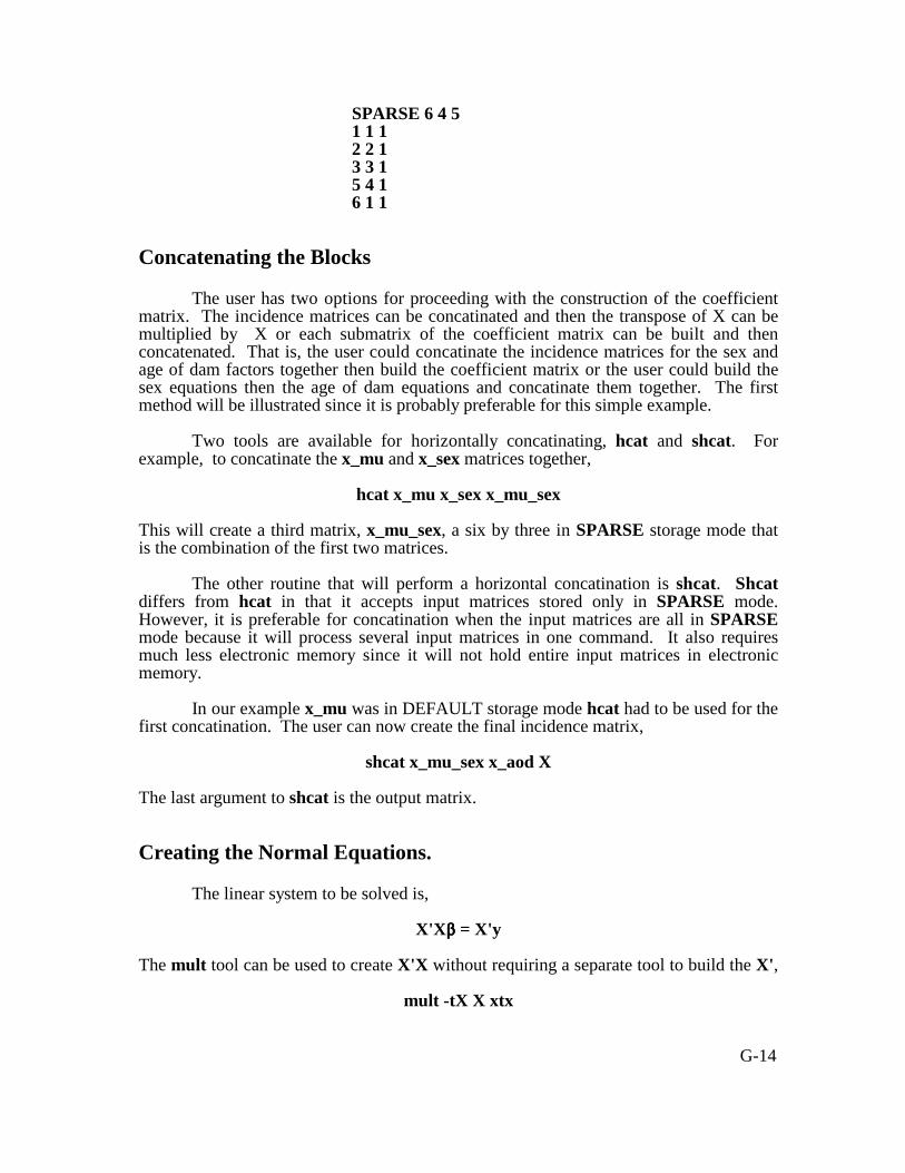
G-14

SPARSE 6 4 51 1 12 2 13 3 15 4 16 1 1

Concatenating the Blocks

The user has two options for proceeding with the construction of the coefficientmatrix. The incidence matrices can be concatinated and then the transpose of X can bemultiplied by X or each submatrix of the coefficient matrix can be built and thenconcatenated. That is, the user could concatinate the incidence matrices for the sex andage of dam factors together then build the coefficient matrix or the user could build thesex equations then the age of dam equations and concatinate them together. The firstmethod will be illustrated since it is probably preferable for this simple example.

Two tools are available for horizontally concatinating, hcat and shcat. Forexample, to concatinate the x_mu and x_sex matrices together,

hcat x_mu x_sex x_mu_sex

This will create a third matrix, x_mu_sex, a six by three in SPARSE storage mode thatis the combination of the first two matrices.

The other routine that will perform a horizontal concatination is shcat. Shcatdiffers from hcat in that it accepts input matrices stored only in SPARSE mode.However, it is preferable for concatination when the input matrices are all in SPARSEmode because it will process several input matrices in one command. It also requiresmuch less electronic memory since it will not hold entire input matrices in electronicmemory.

In our example x_mu was in DEFAULT storage mode hcat had to be used for thefirst concatination. The user can now create the final incidence matrix,

shcat x_mu_sex x_aod X

The last argument to shcat is the output matrix.

Creating the Normal Equations.

The linear system to be solved is,

X'X$$$$ = X'y

The mult tool can be used to create X'X without requiring a separate tool to build the X',

mult -tX X xtx

G-15

The "-t" parameter flag indicates transposition of X before performing the multiplication.The right hand side of the linear system is also constructed with the mult tool,

mult -tX yw xtyw

Now that the normal equations have been constructed, all that is left to do is toimpose constraints on the equations and solve the linear system. Constraint setting andsolution methods for linear systems are discussed in section eight of the Users Guide.

G-16

5 Assembling Single TraitAnimal Models

Several tools are available for building equation systems with both fixed andrandom factors with differing covariance structures between the levels of the randomfactors. This section demonstrates the basic methods and tools for assembling aparticular type of random factor linear system that is commonly called the "single traitanimal model". These techniques will be extrapolated to more complex random factoranalyses in the succeeding sections of this guide.

For the discussion in this section additional information must be added to theexample data file used in the previous sections. A field for sire and dam of the animalwho is represented by each item is included,

A . . 1 5 500B . . 2 3 450C A B 1 2 475D . B 1 5 .E C . 2 4 425F A E 2 5 490

The linear model now becomes,

y = X$$$$ + Zu + e

where u is a vector of random effects on y and Z relates those effects to observations iny. The values in u are typically called breeding values and represent the effects due toadditive gene action (breeding values). The variance structure of u is,

var[u] = AF2

a

where A is the matrix of Wright's numerator relationships and F2a is the variance of the

additive genetic effects.

The normal equations are,

Constructing the Inverse NumeratorRelationship Matrix

G-17

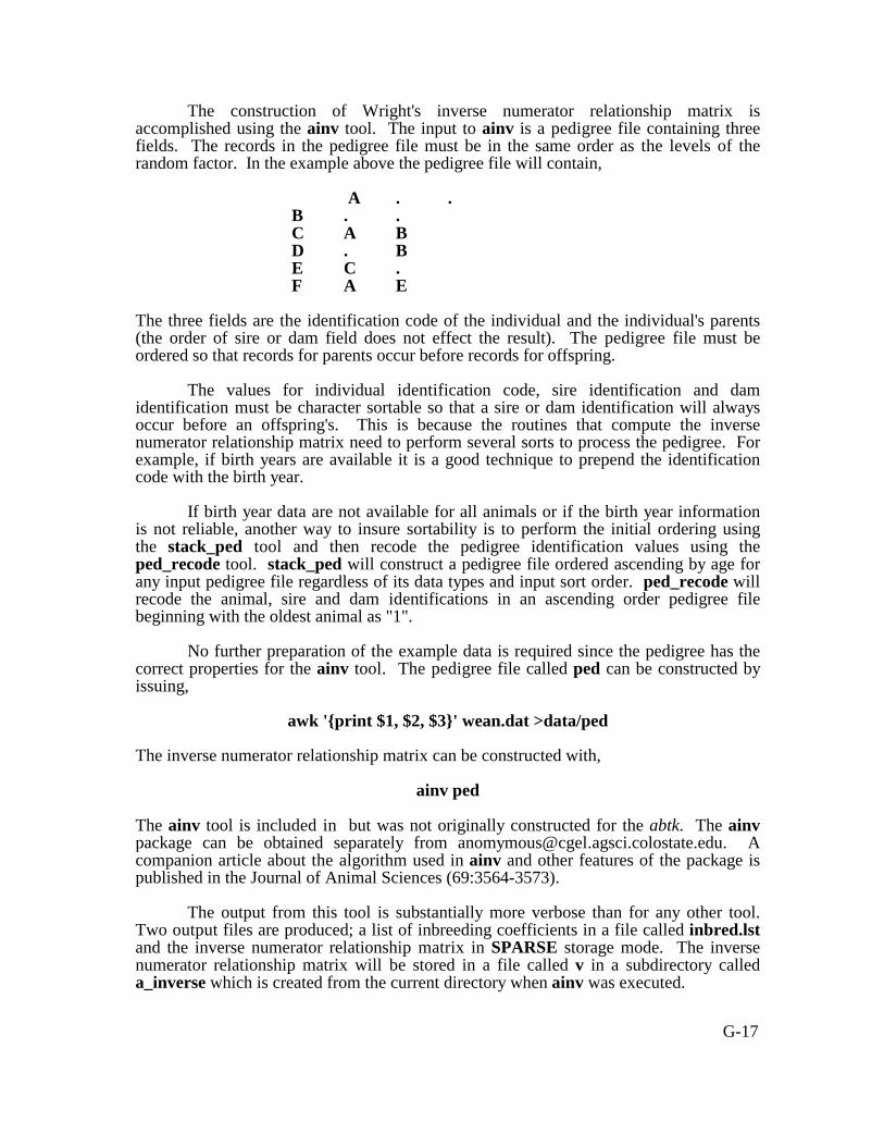
The construction of Wright's inverse numerator relationship matrix isaccomplished using the ainv tool. The input to ainv is a pedigree file containing threefields. The records in the pedigree file must be in the same order as the levels of therandom factor. In the example above the pedigree file will contain,

A . . B . . C A B D . B E C . F A E

The three fields are the identification code of the individual and the individual's parents(the order of sire or dam field does not effect the result). The pedigree file must beordered so that records for parents occur before records for offspring.

The values for individual identification code, sire identification and damidentification must be character sortable so that a sire or dam identification will alwaysoccur before an offspring's. This is because the routines that compute the inversenumerator relationship matrix need to perform several sorts to process the pedigree. Forexample, if birth years are available it is a good technique to prepend the identificationcode with the birth year.

If birth year data are not available for all animals or if the birth year informationis not reliable, another way to insure sortability is to perform the initial ordering usingthe stack_ped tool and then recode the pedigree identification values using theped_recode tool. stack_ped will construct a pedigree file ordered ascending by age forany input pedigree file regardless of its data types and input sort order. ped_recode willrecode the animal, sire and dam identifications in an ascending order pedigree filebeginning with the oldest animal as "1".

No further preparation of the example data is required since the pedigree has thecorrect properties for the ainv tool. The pedigree file called ped can be constructed byissuing,

awk '{print $1, $2, $3}' wean.dat >data/ped

The inverse numerator relationship matrix can be constructed with,

ainv ped

The ainv tool is included in but was not originally constructed for the abtk. The ainvpackage can be obtained separately from anomymous@cgel.agsci.colostate.edu. Acompanion article about the algorithm used in ainv and other features of the package ispublished in the Journal of Animal Sciences (69:3564-3573).

The output from this tool is substantially more verbose than for any other tool.Two output files are produced; a list of inbreeding coefficients in a file called inbred.lstand the inverse numerator relationship matrix in SPARSE storage mode. The inversenumerator relationship matrix will be stored in a file called v in a subdirectory calleda_inverse which is created from the current directory when ainv was executed.

G-18

Assembling the Normal Equations

There are two tools that can be used to assemble the Z matrix for a model withanimal effects. The generalized incidence matrix builder tool, gen_z, can be used buta special tool has been programmed for animal model incedence matrix construction,anim_z. The anim_z tool is preferable because it is substantially faster and does notconsume as much electronic memory to process.

To construct the random effect incidence matrix for the example,

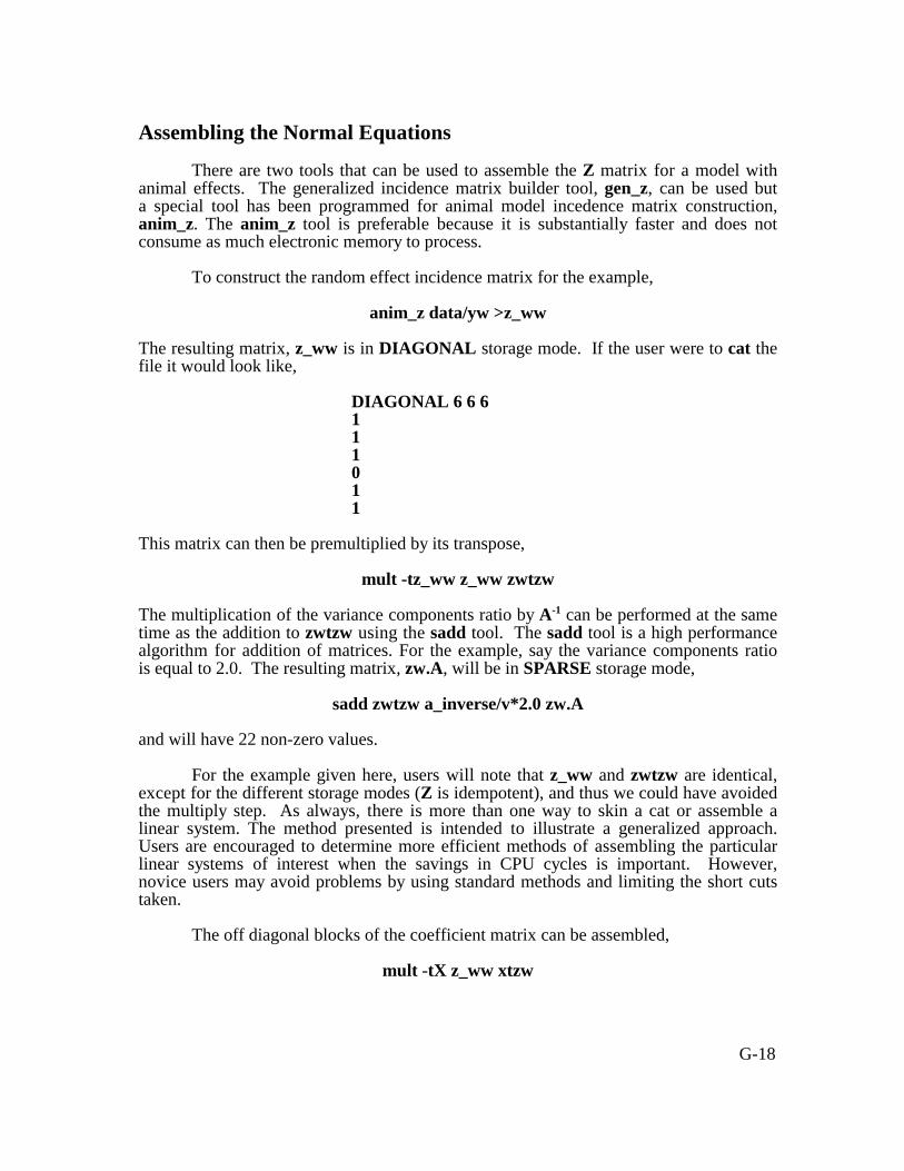
anim_z data/yw >z_ww

The resulting matrix, z_ww is in DIAGONAL storage mode. If the user were to cat thefile it would look like,

DIAGONAL 6 6 6111011

This matrix can then be premultiplied by its transpose,

mult -tz_ww z_ww zwtzw

The multiplication of the variance components ratio by A-1 can be performed at the sametime as the addition to zwtzw using the sadd tool. The sadd tool is a high performancealgorithm for addition of matrices. For the example, say the variance components ratiois equal to 2.0. The resulting matrix, zw.A, will be in SPARSE storage mode,

sadd zwtzw a_inverse/v*2.0 zw.A

and will have 22 non-zero values.

For the example given here, users will note that z_ww and zwtzw are identical,except for the different storage modes (Z is idempotent), and thus we could have avoidedthe multiply step. As always, there is more than one way to skin a cat or assemble alinear system. The method presented is intended to illustrate a generalized approach.Users are encouraged to determine more efficient methods of assembling the particularlinear systems of interest when the savings in CPU cycles is important. However,novice users may avoid problems by using standard methods and limiting the short cutstaken.

The off diagonal blocks of the coefficient matrix can be assembled,

mult -tX z_ww xtzw

G-19

The transpose of xtzw can be taken using the trans tool. However, because of the highspeed performance of the mult algorithm, mult is more efficient for problems withtypical sizes,

mult -tz_ww X zwtx

The mult tool will produce matrices that are in SPARSE storage mode and theresulting matrices can be concatinated using shcat and svcat,

shcat xtx xtzw x.EQ shcat zwtx z.A z.EQ

and

svcat x.EQ z.EQ coef

The right hand side can also be assembled in a similar manner,

mult -tz_ww yw zwtywsvcat xtyw zwtyw RHS

The completed coefficient matrix is coef and the right hand side vector is RHS. Thesolution of this linear system will be discussed in section G-8.

G-20

Maternal Effects Model

Adding maternal effects to the example is a relatively trivial task using the abtk. The model now becomes,

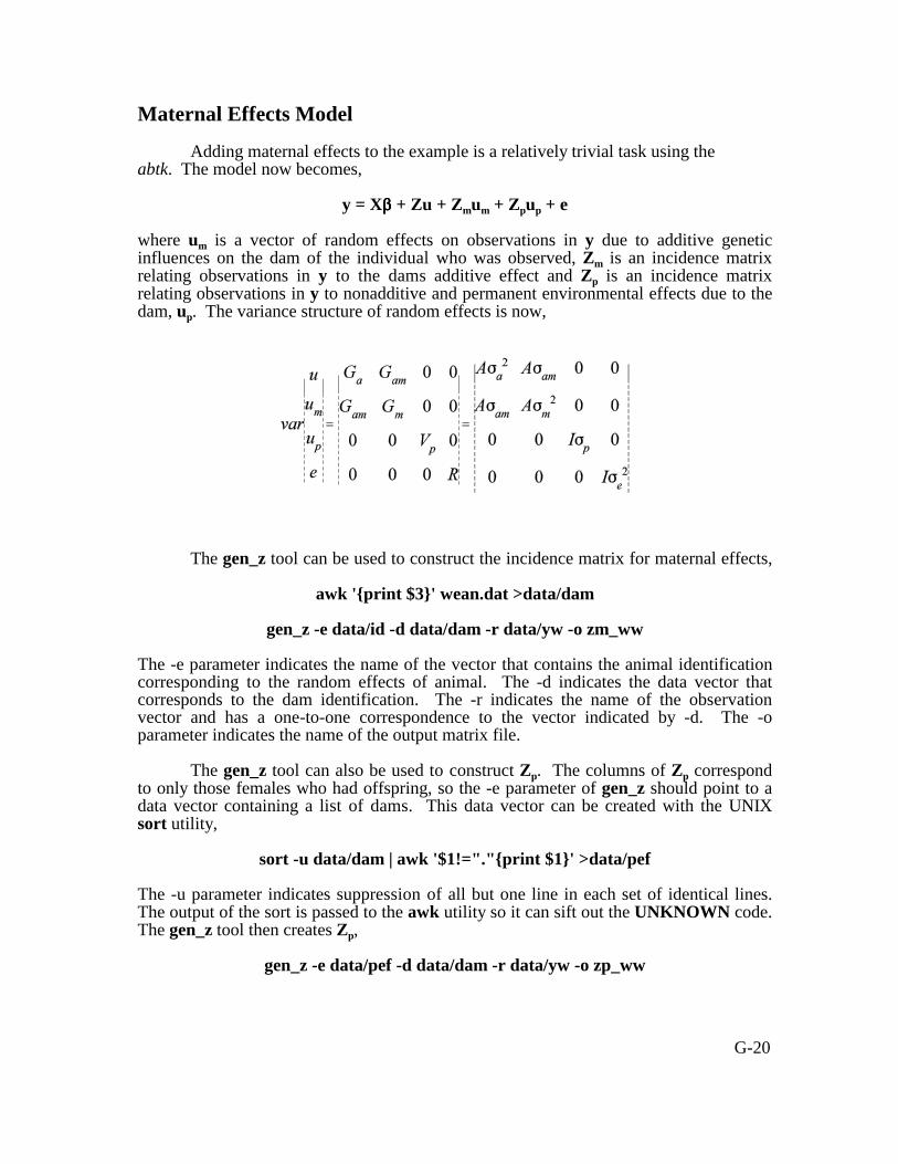
y = X$$$$ + Zu + Zmum + Zpup + e

where um is a vector of random effects on observations in y due to additive geneticinfluences on the dam of the individual who was observed, Zm is an incidence matrixrelating observations in y to the dams additive effect and Zp is an incidence matrixrelating observations in y to nonadditive and permanent environmental effects due to thedam, up. The variance structure of random effects is now,

The gen_z tool can be used to construct the incidence matrix for maternal effects,

awk '{print $3}' wean.dat >data/dam

gen_z -e data/id -d data/dam -r data/yw -o zm_ww

The -e parameter indicates the name of the vector that contains the animal identificationcorresponding to the random effects of animal. The -d indicates the data vector thatcorresponds to the dam identification. The -r indicates the name of the observationvector and has a one-to-one correspondence to the vector indicated by -d. The -oparameter indicates the name of the output matrix file.

The gen_z tool can also be used to construct Zp. The columns of Zp correspondto only those females who had offspring, so the -e parameter of gen_z should point to adata vector containing a list of dams. This data vector can be created with the UNIXsort utility,

sort -u data/dam | awk '$1!="."{print $1}' >data/pef

The -u parameter indicates suppression of all but one line in each set of identical lines.The output of the sort is passed to the awk utility so it can sift out the UNKNOWN code.The gen_z tool then creates Zp,

gen_z -e data/pef -d data/dam -r data/yw -o zp_ww

G-21

Maternal Effects Normal Equations

One set of normal equations for the maternal effects model is,

where,

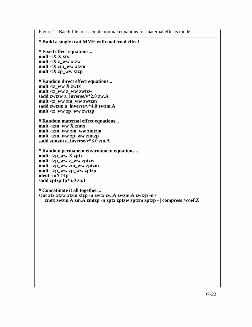
Assembling equations using a script file. The components can be assembled usingthe mult, sadd, shcat and svcat tools. These commands can be placed into a file usinga UNIX editor such as vi and executed as a batch file in background. Figure 1 shows anexample script file for building the normal equations for the model with maternal effects.If this file were named "mkcoef", it could be run in background by issuing,

sh mkcoef &

the "&" indicates background processing of the script file. The "sh" is the UNIX bourneshell command processor.

G-22

Figure 1. Batch file to assemble normal equations for maternal effects model. # Build a single trait MME with maternal effect

# Fixed effect equations...mult -tX X xtxmult -tX z_ww xtzw mult -tX zm_ww xtzmmult -tX zp_ww xtzp

# Random direct effect equations...mult -tz_ww X zwtxmult -tz_ww z_ww zwtzwsadd zwtzw a_inverse/v*2.0 zw.Amult -tz_ww zm_ww zwtzmsadd zwtzm a_inverse/v*4.0 zwzm.Amult -tz_ww zp_ww zwtzp

# Random maternal effect equations...mult -tzm_ww X zmtxmult -tzm_ww zm_ww zmtzmmult -tzm_ww zp_ww zmtzpsadd zmtzm a_inverse/v*3.0 zm.A

# Random permanent environment equations...mult -tzp_ww X zptxmult -tzp_ww z_ww zptzwmult -tzp_ww zm_ww zptzmmult -tzp_ww zp_ww zptzpident -mX >Ipsadd zptzp Ip*5.0 zp.I

# Concatinate it all together...scat xtx xtzw xtzm xtzp -n zwtx zw.A zwzm.A zwtzp -n \ zmtx zwzm.A zm.A zmtzp -n zptx zptzw zptzm zptzp - | compress >coef.Z

G-23

6 Assembling Reduced Animal Models

The normal equations for assembling a reduced animal model can be expressedin two ways. Many researchers represent the incidence matrix for non-parent randomeffects using a separate incidence matrix, usually P. So now Z becomes the incidencematrix relating the random additive effects of only parent animals to their observations.However, it is easier to conceptualize the model and construct it with the abtk if the Zmatrix represents both parent and nonparent observations and P is not considered. Thisis the method used by Quaas and Pollak (1980, Journ. Anim. Sci 51:1277) to express thelinear system for RAM. It has the additional advantage of using the same notationalmethod of expressing the normal equations as does the model with animal effects. Forexample, after manipulating the algebra the animal model normal equations can beexpressed as,

Z, A-1, u and R-1 are redefined for the reduced animal model.

The Z matrix for random additive effects in the example would be,

The columns of Z correspond to the four animals who became parents, A, B, Cand E. This incidence matrix can be constructed using the ram_z tool,

ram_z -i data/id -s data/sires -d data/dams -e parents -r data/yw -o zr_ww

where data/id is the vector of animal identifications from the data, data/sires is the vectorof sires from the data and data/dams is the vector of dam identifications from the data.These three vectors can be constructed using awk. They have a one-to-onecorrespondence to the observation vector data/yw. The parents vector is a listing of theparent identifications that correspond to the columns of the incidence matrix. It is an

G-24

input vector that can be constructed by passing a list of all parents to the sort utility andsorting it with a -u parameter (sifting out the UNKNOWN code, see section 5 of theUsers Guide). This vector should have a one to one correspondence with the A-1 matrix.

The R-1 has a different structure then the R-1 used for a full animal model set ofnormal equations. The residual variance of non-parents includes the sampling variance.A special tool, form_rr, will construct R-1 for a reduced animal model. Form_rr canconstruct an inverse residual matrix for a single trait model or it will construct the threeblocks of the inverse required for a two trait model (see section G7). For the single traitexample discussed in this section R-1 can be formed by,

form_rr -r 50.0 -g 25.0 -i data/id -p parents -1 data/yw Ri

where the argument to the -r parameter is the residual variance (50.0), the argument tothe -g parameter is the additive genetic variance (25.0). The -i indicates the name of theanimal identification vector from the data, -p indicates the name of the vector thatcontains the parent identifications that corresponds to the columns of the incidencematrix, -1 indicates the name of the observation vector. The last argument is the nameof the file where the inverse residual matrix will be stored.

It is important to point out that form_rr assumes a relationship coefficient of .5between offspring and parent when constructing the inverse residual variance matrix.This may influence an individual researchers decision to construct a full animal modelinstead a reduced animal model.

The A-1 becomes the relationship matrix for only animals who became parents.Therefore, a pedigree file must be constructed for the parents vector. This can be easilyaccomplished using the UNIX join utility. For example, the script in figure 2 willconstruct a pedigree file for parents (par_ped) only from the pedigree file called ped.

# Form parents only pedigree file.

awk '{printf "%s\n%s\n", $2, $3}' ped | sort -u | awk '$1!= "."{print $1}' >tmp1sort ped | join -a1 -e "." -o 1.1 2.2 2.3 tmp1 - >tmp2stack_ped tmp2 >par_pedrm tmp1 tmp2

Figure 2. Script to form a pedigree file for parents only from a complete pedigree file.

Forming the Normal Equations

Assembling the normal equations proceeds as discussed in section G5 with oneexception. The assembly of the blocks of the normal equations to include R-1 can occurin one command instead of requiring two separate mult commands. For example, toassemble,

Z'R-1X

a single mult can be issued,

G-25

mult -tzr_ww*Ri X zrtx

The mult tool uses a high performance algorithm that takes advantage of theDIAGONAL storage mode of Ri and the SPARSE storage modes of zr_ww and X. Theremainder of the assembly proceeds as discussed before.

G-26

7 Assembling Multiple TraitModels

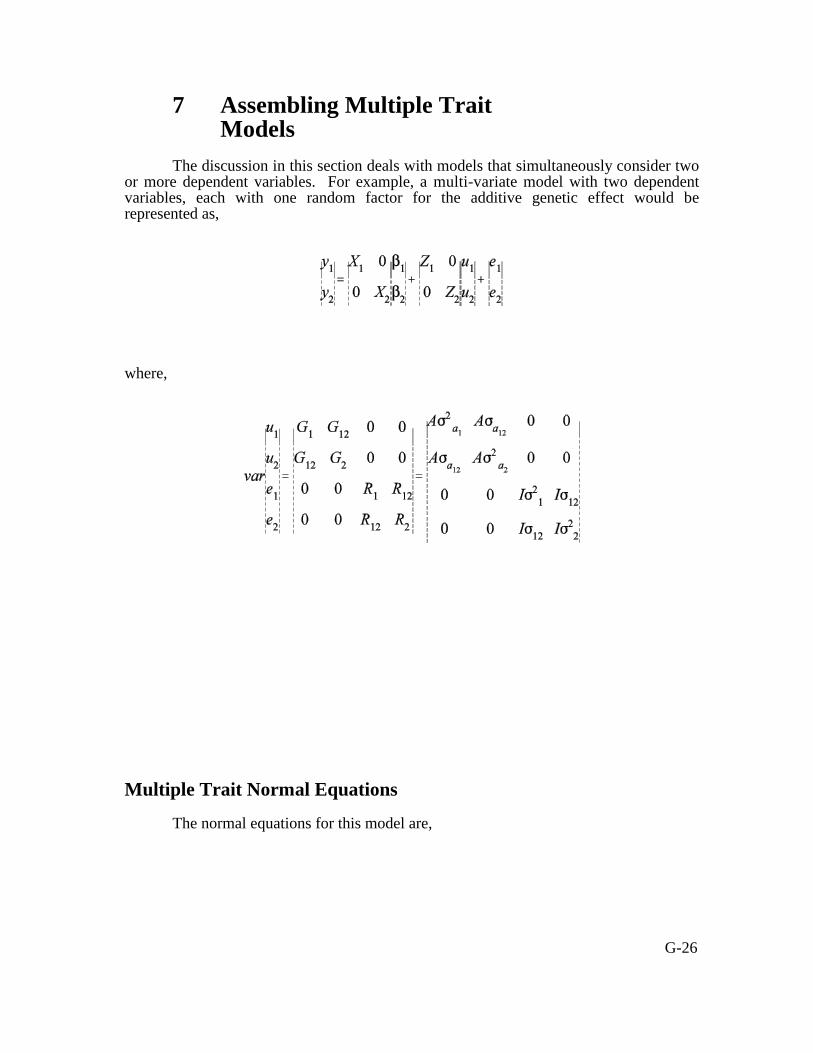
The discussion in this section deals with models that simultaneously consider twoor more dependent variables. For example, a multi-variate model with two dependentvariables, each with one random factor for the additive genetic effect would berepresented as,

where,

Multiple Trait Normal Equations

The normal equations for this model are,

G-27

Inverse Residual Matrix Blocks

The only tool required to assemble a multiple trait full animal model that has notalready been discussed is form_r. The form_r tool works like the form_rr tool for thereduced animal model only it assembles the block matrices for a two trait inverseresidual variance matrix for a full animal model. Users will realize that form_r, as withseveral of the tools is generalizable. It can be used to construct residual variancematrices for models that have other random factors besides animal. Such models includeherd effects, sire effects or sire and dam effects. 22

RAM Multiple Trait Models

As discussed in section six of the Users Guide, reduced animal models can berepresented using the same matrix algebra symbols as full animal models. The onlythings that need to change are the definitions of the random factor incidence matrices,the inverse residual variance matrix and the inverse numerator relationship matrix.

When assembling the multiple trait RAM the random factor incidence matriceswould each be assembled the same way as for a single trait RAM. The only matrix thatchanges substantially is the inverse residual matrix. The reader is encouraged to seeQuaas and Pollak (1980 JAS 51:1277) for a complete treatment of the subject. Theform_rr tool was used to assemble R-1 for the single trait RAM in section six of theUsers Guide. The form_rr tool can also be used to construct the three blocks of themultiple-trait RAM,

The user should refer to the reference manual page to see this syntax. The user is alsoencourage to see the example scripts that come with the abtk and are given in theappendix of this guide.

G-28

G-29

8 Solving The Linear SystemThe current release of the abtk comes with a direct solver and an iterative solver

routine. Both methods of solution are best suited for linear systems. It is possible toconstruct non-linear systems or optimization systems using the abtk. Users are highlyencouraged to develop source codes to work with these types of systems and distributethese codes to their colleagues through the anonymous FTP at cgel.agsci.colostate.edu.

Direct Solution Using an Inverse

Inverting the coefficient matrix of a linear system can be a very computationallyintensive procedure, even for relatively small systems of equations. The invert tool, likeall other abtk tools, uses dynamic memory allocation. Therefore problem size is limitedby available memory. However, practically the problem size is also limited byprocessing time and precision of arithmetic used by the C language compiler that builtthe toolkit. Unfortunately, the inverse is required for the prediction error variance of thesolutions. Current approximation methods for prediction error variance are not adequatefor many mixed models, particularly when variance components are being estimatedusing procedures such as REML.

Not many realistic mixed model linear systems can be solved directly using eventhe largest compute architectures currently available. However, the rapid pace of changein computing technology will continue to allow the user to increase problem sizes suitedfor direct solution. Users are encouraged to inspect the "CHANGES" file at theanonymous FTP at cgel.agsci.colostate.edu regularly to be informed about updates to theabtk.

The invert tool can take a direct inverse or a generalized inverse of a matrix.

Iterative Solution

An iterative solution can be obtained to the linear system using the itgen tool.itgen uses a Gauss-Siedel iteration strategy. Users are encouraged to see the referencemanual page to see the optional variations on the iterative method that may speedconvergence for their linear system.

Imposing constraints for an iterative solution. Van Vleck (personalcommunication, 1990) indicates that it is not necessary to impose constraints on linearsystems that have dependencies when computing an iterative solution. The valuesobtained for fixed effects may look well outside the parameter space, but the differencesbetween the values still have the same expectations. However, it is advantageous toimpose constraints on fixed effects because it reduces the total number of non-zeroelements processed. Additionally, if the equations eliminated are chosen carefully thediagonal dominance of the linear system can be substantially increased, and thus, thetotal number of rounds required to obtain a converged solution can be decreased.

A very practical constraint to impose is the elimination of the equation for themean. This equation is the most dense and usually slows the rate of convergence.Another reason to eliminate the equation for the mean is that the easiest way to eliminate

G-30

it would be to never build it. This way the user can avoid processing all non-zero valuesthrough the entire assembly phase.

However, the example given here from the linear system constructed in sectionsfour and five of the Users Guide does not eliminate the equation for the mean. Insteadthe constraints imposed are to eliminate the equations for the last level (class) of the twofixed effects, sex and age of dam. This is the type of constraint typically imposed byPROC GLM of the SAS procedures (1990). The solutions for the other levels of eacheffect are then the deviations from the last level. The last levels of the sex and age ofdam factors are in equations three and seven, respectively. The genrliz tool will imposethe constraints

genrlz -c coef -n coef_g -r RHS -R RHS_g 3 7

Solving the linear system. To compute five hundred rounds of Gauss-Siedeliteration for the example problem assembled in section five of the Users Guide andconstrained above, the invocation of itgen would be,

itgen -m 500 -r RHS_g -b beta -n coef_g

The -m parameter indicates the number of rounds to iterate, the -r parameter indicatesthe name of the right hand side vector, -n indicates the name of the coefficient matrixand -b indicates the name of the solution vector, in this example "beta". Additionally,there is an optional restart parameter, -R, who's argument indicates the name of a vectorto use as starting values.

The current implementation of itgen does not have a stopping criteria other thanthe -m parameter. It was determined that convergence criteria were too costly tocompute and yielded too little information about the behavior of the linear system.Users can compute convergence values such as the residual variance or genetic trend,in between sets of iteration and restart itgen as needed. There is a weak convergencecriteria printed to standard error that is useful in indicating if the solutions are diverging.This criteria is the average change in all solutions.

The order of the values in the solution vector file will be the same order that thelinear system was assembled. For the example, the first value in beta will be thesolution to the equation for the mean. The second value will be the solutioncorresponding to sex code 1. Its expectation will be the effect of sex 1 minus the effectof sex 2. The third value will be a zero because equation three was eliminated. Valuesin the fourth through the sixth rows will be solutions for age of dam categories 5, 3 and2 respectively. This is the order that the fef tool constructed the incidence matrix andcorresponds to the order of values in the a.list file (see section four of the Users Guide).The expectations of these solutions are the deviation of the effects from the last effect.The value in row seven is zero since its equation was eliminated to break thedependencies. The remaining values are "breeding values" of the animals in the orderthey appear in the pedigree file.