arX

iv:q

uant

-ph/

0105

127v

3 1

9 Ju

n 20

03

DECOHERENCE, EINSELECTION,

AND THE QUANTUM ORIGINS OF THE CLASSICAL

Wojciech Hubert Zurek

Theory Division, LANL, Mail Stop B288

Los Alamos, New Mexico 87545

Decoherence is caused by the interaction with the en-vironment which in effect monitors certain observablesof the system, destroying coherence between the pointer

states corresponding to their eigenvalues. This leadsto environment-induced superselection or einselection, aquantum process associated with selective loss of infor-mation. Einselected pointer states are stable. They canretain correlations with the rest of the Universe in spiteof the environment. Einselection enforces classicality byimposing an effective ban on the vast majority of theHilbert space, eliminating especially the flagrantly non-local “Schrodinger cat” states. Classical structure ofphase space emerges from the quantum Hilbert space inthe appropriate macroscopic limit: Combination of einse-lection with dynamics leads to the idealizations of a pointand of a classical trajectory. In measurements, einselec-tion replaces quantum entanglement between the appa-ratus and the measured system with the classical corre-lation. Only the preferred pointer observable of the ap-paratus can store information that has predictive power.When the measured quantum system is microscopic andisolated, this restriction on the predictive utility of itscorrelations with the macroscopic apparatus results inthe effective “collapse of the wavepacket”. Existential in-

terpretation implied by einselection regards observers asopen quantum systems, distinguished only by their abil-ity to acquire, store, and process information. Spreadingof the correlations with the effectively classical pointerstates throughout the environment allows one to under-stand ‘classical reality’ as a property based on the rela-

tively objective existence of the einselected states: Theycan be “found out” without being re-prepared, e.g, byintercepting the information already present in the envi-ronment. The redundancy of the records of pointer statesin the environment (which can be thought of as their ‘fit-ness’ in the Darwinian sense) is a measure of their clas-sicality. A new symmetry appears in this setting: Envi-ronment - assisted invariance or envariance sheds a newlight on the nature of ignorance of the state of the systemdue to quantum correlations with the environment, andleads to Born’s rules and to the reduced density matri-ces, ultimately justifying basic principles of the programof decoherence and einselection.

Contents

I. INTRODUCTION 2

A. The problem: Hilbert space is big 21. Copenhagen Interpretation 22. Many Worlds Interpretation 3

B. Decoherence and einselection 3C. The nature of the resolution and the role of envariance4

D. Existential Interpretation and ‘Quantum Darwinism’4

II. QUANTUM MEASUREMENTS 5A. Quantum conditional dynamics 5

1. Controlled not and a bit-by-bit measurement 62. Measurements and controlled shifts. 73. Amplification 7

B. Information transfer in measurements 91. Action per bit 9

C. “Collapse” analogue in a classical measurement 9

III. CHAOS AND LOSS OF CORRESPONDENCE 11A. Loss of the quantum-classical correspondence 11B. Moyal bracket and Liouville flow 12C. Symptoms of correspondence loss 13

1. Expectation values 132. Structure saturation 13

IV. ENVIRONMENT – INDUCED SUPERSELECTION14

A. Models of einselection 141. Decoherence of a single qubit 152. The classical domain and a quantum halo 163. Einselection and controlled shifts 16

B. Einselection as the selective loss of information 171. Mutual information and discord 18

C. Decoherence, entanglement, dephasing, and noise 19D. Predictability sieve and einselection 20

V. EINSELECTION IN PHASE SPACE 21A. Quantum Brownian motion 21B. Decoherence in quantum Brownian motion 23

1. Decoherence timescale 242. Phase space view of decoherence 25

C. Predictability sieve in phase space 26D. Classical limit in phase space 26

1. Mathematical approach (h→ 0) 272. Physical approach: The macroscopic limit 273. Ignorance inspires confidence in classicality 28

E. Decoherence, chaos, and the Second Law 281. Restoration of correspondence 282. Entropy production 293. Quantum predictability horizon 30

VI. EINSELECTION AND MEASUREMENTS 30A. Objective existence of einselected states 30B. Measurements and memories 31C. Axioms of quantum measurement theory 32

1. Observables are Hermitean – axiom (iiia) 322. Eigenvalues as outcomes – axiom (iiib) 333. Immediate repeatability, axiom (iv) 334. Probabilities, einselection and records 34

2

D. Probabilities from Envariance 341. Envariance 352. Born’s rule from envariance 363. Relative frequencies from envariance 384. Other approaches to probabilities 39

VII. ENVIRONMENT AS A WITNESS 40A. Quantum Darwinism 40

1. Consensus and algorithmic simplicity 412. Action distance 413. Redundancy and mutual information 424. Redundancy ratio rate 43

B. Observers and the Existential Interpretation 43C. Events, Records, and Histories 44

1. Relatively Objective Past 45

VIII. DECOHERENCE IN THE LABORATORY 46A. Decoherence due to entangling interactions 46B. Simulating decoherence with classical noise 47

1. Decoherence, Noise, and Quantum Chaos 48C. Analogue of decoherence in a classical system 48D. Taming decoherence 49

1. Pointer states and noiseless subsystems 492. Environment engineering 493. Error correction and resilient computing 50

IX. CONCLUDING REMARKS 51

X. ACKNOWLEDGMENTS 52

References 52

I. INTRODUCTION

The issue of interpretation is as old as quantum the-ory. It dates back to the discussions of Niels Bohr,Werner Heisenberg, Erwin Schrodinger, (Bohr, 1928;1949; Heisenberg, 1927; Schrodinger, 1926; 1935a,b; seealso Jammer, 1974; Wheeler and Zurek, 1983). Perhapsthe most incisive critique of the (then new) theory wasdue to Albert Einstein, who, searching for inconsisten-cies, distilled the essence of the conceptual difficulties ofquantum mechanics through ingenious “gedankenexper-iments”. We owe him and Bohr clarification of the sig-nificance of the quantum indeterminacy in course of theSolvay congress debates (see Bohr, 1949) and elucidationof the nature of quantum entanglement (Einstein, Podol-sky, and Rosen, 1935; Bohr, 1935, Schrodinger, 1935a,b).Issues identified then are still a part of the subject.

Within the past two decades the focus of the re-search on the fundamental aspects of quantum theory hasshifted from esoteric and philosophical to more “down toearth” as a result of three developments. To begin with,many of the old gedankenexperiments (such as the EPR“paradox”) became compelling demonstrations of quan-tum physics. More or less simultaneously the role of de-coherence begun to be appreciated and einselection wasrecognized as key in the emergence of classicality. Lastnot least, various developments have led to a new viewof the role of information in physics. This paper reviewsprogress with a focus on decoherence, einselection andthe emergence of classicality, but also attempts a “pre-view” of the future of this exciting and fundamental area.

A. The problem: Hilbert space is big

The interpretation problem stems from the vastness ofthe Hilbert space, which, by the principle of superposi-tion, admits arbitrary linear combinations of any statesas a possible quantum state. This law, thoroughly testedin the microscopic domain, bears consequences that defyclassical intuition: It appears to imply that the familiarclassical states should be an exceedingly rare exception.And, naively, one may guess that superposition principleshould always apply literally: Everything is ultimatelymade out of quantum “stuff”. Therefore, there is noa priori reason for macroscopic objects to have definiteposition or momentum. As Einstein noted1 localizationwith respect to macrocoordinates is not just independent,but incompatible with quantum theory. How can one thenestablish correspondence between the quantum and thefamiliar classical reality?

1. Copenhagen Interpretation

Bohr’s solution was to draw a border between thequantum and the classical and to keep certain objects –especially measuring devices and observers – on the clas-sical side (Bohr, 1928; 1949). The principle of superposi-tion was suspended “by decree” in the classical domain.The exact location of this border was difficult to pinpoint,but measurements “brought to a close” quantum events.Indeed, in Bohr’s view the classical domain was morefundamental: Its laws were self-contained (they could beconfirmed from within) and established the frameworknecessary to define the quantum.

The first breach in the quantum-classical border ap-peared early: In the famous Bohr – Einstein double-slitdebate, quantum Heisenberg uncertainty was invoked byBohr at the macroscopic level to preserve wave-particleduality. Indeed, as the ultimate components of classicalobjects are quantum, Bohr emphasized that the bound-ary must be moveable, so that even the human nervoussystem could be regarded as quantum provided that suit-able classical devices to detect its quantum features wereavailable. In the words of John Archibald Wheeler (1978;1983) who has elucidated Bohr’s position and decisivelycontributed to the revival of interest in these matters,“No [quantum] phenomenon is a phenomenon until it isa recorded (observed) phenomenon”.

1 In a letter dated 1954, Albert Einstein wrote to Max Born “Letψ1 and ψ2 be solutions of the same Schrodinger equation.. . ..When the system is a macrosystem and when ψ1 and ψ2 are‘narrow’ with respect to the macrocoordinates, then in by far thegreater number of cases this is no longer true for ψ = ψ1 + ψ2.Narrowness with respect to macrocoordinates is not only inde-pendent of the principles of quantum mechanics, but, moreover,incompatible with them.” (The translation from Born (1969)quoted here is due to Joos (1986).)

3

This is a pithy summary of a point of view – known asthe Copenhagen Interpretation (CI) – that has kept manya physicist out of despair. On the other hand, as long as acompelling reason for the quantum-classical border couldnot be found, the CI Universe would be governed by twosets of laws, with poorly defined domains of jurisdiction.This fact has kept many a student, not to mention theirteachers, in despair (Mermin 1990a; b; 1994).

2. Many Worlds Interpretation

The approach proposed by Hugh Everett (1957a, b)and elucidated by Wheeler (1957), Bryce DeWitt (1970)and others (see DeWitt and Graham, 1973; Zeh, 1970;1973; Geroch, 1984; Deutsch, 1985, 1997, 2001) was toenlarge the quantum domain. Everything is now repre-sented by a unitarily evolving state vector, a gigantic su-perposition splitting to accommodate all the alternativesconsistent with the initial conditions. This is the essenceof the Many Worlds Interpretation (MWI). It does notsuffer from the dual nature of CI. However, it also doesnot explain the emergence of classical reality.

The difficulty many have in accepting MWI stems fromits violation of the intuitively obvious “conservation law”– that there is just one Universe, the one we perceive.But even after this question is dealt with, , many a con-vert from CI (which claims allegiance of a majority ofphysicists) to MWI (which has steadily gained popular-ity; see Tegmark and Wheeler, 2001, for an assessment)eventually realizes that the original MWI does not ad-dress the “preferred basis question” posed by Einstein1

(see Wheeler, 1983; Stein, 1984; Bell 1981, 1987; Kent,1990; for critical assessments of MWI). And as long asit is unclear what singles out preferred states, perceptionof a unique outcome of a measurement and, hence, of asingle Universe cannot be explained either2.

In essence, Many Worlds Interpretation does not ad-dress but only postpones the key question. The quantum- classical boundary is pushed all the way towards theobserver, right against the border between the materialUniverse and the “consciousness”, leaving it at a veryuncomfortable place to do physics. MWI is incomplete:It does not explain what is effectively classical and why.Nevertheless, it was a crucial conceptual breakthrough:

2 DeWitt, in the Many Worlds re-analysis of quantum measure-ments makes this clear: in DeWitt and Graham (1973), lastparagraph of p. 189 he writes about the key ‘remaining prob-lem’: “Why is it so easy to find apparata in states [with a welldefined value of the pointer observable]? In the case of macro-scopic apparata it is well known that a small value for the meansquare deviation of a macroscopic observable is a fairly stableproperty of the apparatus. But how does the mean square devi-ation become so small in the first place? Why is a large value ofthe mean square deviation of a macroscopic observable virtuallynever, in fact, encountered in practice? . . . a proof of this doesnot yet exist. It remains a program for the future.”

Everett reinstated quantum mechanics as a basic tool inthe search for its interpretation.

B. Decoherence and einselection

Decoherence and einselection are two complementaryviews of the consequences of the same process of envi-ronmental monitoring. Decoherence is the destructionof quantum coherence between preferred states associ-ated with the observables monitored by the environment.Einselection is its consequence – the de facto exclusionof all but a small set, a classical domain consisting ofpointer states – from within a much larger Hilbert space.Einselected states are distinguished by their resilience –stability in spite of the monitoring environment.

The idea that “openness” of quantum systems mayhave anything to do with the transition from quantum toclassical was resolutely ignored for a very long time, prob-ably because in classical physics problems of fundamen-tal importance were always settled in isolated systems. Inthe context of measurements Gottfried (1967) anticipatedsome of the latter developments. The fragility of energylevels of quantum systems was emphasized by seminal pa-pers of Dieter Zeh (1970; 1973), who argued (inspired byremarks relevant to what would be called today “deter-ministic chaos” (Borel, 1914)) that macroscopic quantumsystems are in effect impossible to isolate.

The understanding of how the environment distills theclassical essence from quantum systems is more recent(Zurek, 1981; 1982; 1993a). It combines two observa-tions: (1) In quantum physics “reality” can be attributedto the measured states. (2) Information transfer usuallyassociated with measurements is a common result of al-most any interaction with the environment of a system.

Some quantum states are resilient to decoherence. Thisis the basis of einselection. Using Darwinian analogy,one might say that pointer states are most ‘fit’. Theysurvive monitoring by the environment to leave ‘descen-dants’ that inherit their properties. Classical domain ofpointer states offers a static summary of the result ofquantum decoherence. Save for classical dynamics, (al-most) nothing happens to these einselected states, eventhough they are immersed in the environment.

It is difficult to catch einselection “in action”: Envi-ronment has little effect on the pointer states, as theyare already classical. Therefore, it was easy to missdecoherence - driven dynamics of einselection by tak-ing for granted its result – existence of the classical do-main, and a ban on arbitrary quantum superpositions.Macroscopic superpositions of einselected states disap-pear rapidly. Einselection creates effective superselectionrules (Wick, Wightman and Wigner, 1952; 1970; Wight-man, 1995). However, in the microscopic, decoherencecan be slow in comparison with the dynamics.

Einselection is a quantum phenomenon. Its essencecannot be even motivated classically: In classical physicsarbitrarily accurate measurements (also by the environ-

4

ment) can be in principle carried out without disturbingthe system. Only in quantum mechanics acquisition ofinformation inevitably alters the state of the system –the fact that becomes apparent in double-slit and relatedexperiments (Wootters and Zurek, 1979; Zurek, 1983).

Quantum nature of decoherence and the absence ofclassical analogues are a source of misconceptions. Forinstance, decoherence is sometimes equated with relax-ation or classical noise that can be also introduced bythe environment. Indeed, all of these effects often ap-pear together and as a consequence of the “openness”.The distinction between them can be briefly summed up:Relaxation and noise are caused by the environment per-

turbing the system, while decoherence and einselection

are caused by the system perturbing the environment.Within the past few years decoherence and einselection

became familiar to many. This does not mean that theirimplications are universally accepted (see comments inthe April 1993 issue of Physics Today; d’Espagnat, 1989and 1995; Bub, 1997; Leggett, 1998 and 2002; Stapp,2001; exchange of views between Anderson, 2001, andAdler, 2001). In a field where controversy reigned for solong this resistance to a new paradigm is no surprise.

C. The nature of the resolution and the role of envariance

Our aim is to explain why does the quantum Universeappear classical. This question can be motivated onlyin the context of the Universe divided into systems, andmust be phrased in the language of the correlations be-tween them. In the absence of systems Schrodinger equa-tion dictates deterministic evolution;

|Ψ(t)〉 = exp(−iHt/h) |Ψ(0)〉 , (1.1)

and the problem of interpretation seems to disappear.There is no need for “collapse” in a Universe with no

systems. Yet, the division into systems is imperfect. Asa consequence, the Universe is a collection of open (in-teracting) quantum systems. As the interpretation prob-lem does not arise in quantum theory unless interactingsystems exist, we shall also feel free to assume that anenvironment exists when looking for a resolution.

Decoherence and einselection fit comfortably in thecontext of the Many Worlds Interpretation where theydefine the “branches” of the universal state vector. De-coherence makes MWI complete: It allows one to ana-lyze the Universe as it is seen by an observer, who is alsosubject to decoherence. Einselection justifies elementsof Bohr’s CI by drawing the border between the quan-tum and the classical. This natural boundary can besometimes shifted: Its effectiveness depends on the de-gree of isolation and on the manner in which the systemis probed, but it is a very effective quantum - classicalborder nevertheless.

Einselection fits either MWI or CI framework: It sup-plies a statute of limitations, putting an end to thequantum jurisdiction. . It delineates how much of the

Universe will appear classical to observers who monitorit from within, using their limited capacity to acquire,store, and process information. It allows one to under-stand classicality as an idealization that holds in the limitof macroscopic open quantum systems.

Environment imposes superselection rules by preserv-ing part of the information that resides in the correlationsbetween the system and the measuring apparatus (Zurek,1981, 1982). The observer and the environment competefor the information about the system. Environment –because of its size and its incessant interaction with thesystem – wins that competition, acquiring informationfaster and more completely than the observer. Thus, arecord useful for the purpose of prediction must be re-stricted to the observables that are already monitored bythe environment. In that case, the observer and the en-vironment no longer compete and decoherence becomesunnoticeable. Indeed, typically observers use environ-

ment as a “communication channel”, and monitor it to

find out about the system.Spreading of the information about the system through

the environment is ultimately responsible for the emer-gence of the “objective reality”. Objectivity of a statecan be quantified by the redundancy with which it isrecorded throughout Universe. Intercepting fragments ofthe environment allows observers to find out (pointer)state of the system without perturbing it (Zurek, 1993a,1998a, and 2000; see especially section VII of this pa-per for a preview of this new “environment as a witness”approach to the interpretation of quantum theory).

When an effect of a transformation acting on a systemcan be undone by a suitable transformation acting on theenvironment, so that the joint state of the two remainsunchanged, the transformed property of the system issaid to exhibit “environment assisted invariance” or en-

variance (Zurek, 2002b). Observer must be obviouslyignorant of the envariant properties of the system. Pureentangled states exhibit envariance. Thus, in quantumphysics perfect information about the joint state of thesystem-environment pair can be used to prove ignoranceof the state of the system.

Envariance offers a new fundamental view of what isinformation and what is ignorance in the quantum world.It leads to Born’s rule for the probabilities and justifiesthe use of reduced density matrices as a description of apart of a larger combined system. Decoherence and ein-selection rely on reduced density matrices. Envarianceprovides a fundamental resolution of many of the inter-pretational issues. It will be discussed in section VI D.

D. Existential Interpretation and ‘Quantum Darwinism’

What the observer knows is inseparable from what theobserver is: The physical state of his memory implieshis information about the Universe. Its reliability de-pends on the stability of the correlations with the exter-nal observables. In this very immediate sense decoher-

5

ence enforces the apparent “collapse of the wavepacket”:After a decoherence timescale, only the einselected mem-ory states will exist and retain useful correlations (Zurek,1991; 1998a,b; Tegmark, 2000). The observer describedby some specific einselected state (including a configu-ration of memory bits) will be able to access (“recall”)only that state. The collapse is a consequence of einse-lection and of the one-to-one correspondence between thestate of his memory and of the information encoded in it.Memory is simultaneously a description of the recordedinformation and a part of the “identity tag”, definingobserver as a physical system. It is as inconsistent toimagine observer perceiving something else than what isimplied by the stable (einselected) records in his posses-sion as it is impossible to imagine the same person with adifferent DNA: Both cases involve information encoded ina state of a system inextricably linked with the physicalidentity of an individual.

Distinct memory/identity states of the observer (thatare also his “states of knowledge”) cannot be superposed:This censorship is strictly enforced by decoherence andthe resulting einselection. Distinct memory states labeland “inhabit” different branches of the Everett’s “ManyWorlds” Universe. Persistence of correlations is all that isneeded to recover “familiar reality”. In this manner, thedistinction between epistemology and ontology is washedaway: To put it succinctly (Zurek, 1994) there can be no

information without representation in physical states.

There is usually no need to trace the collapse allthe way to observer’s memory. It suffices that thestates of a decohering system quickly evolve into mix-tures of the preferred (pointer) states. All that can beknown in principle about a system (or about an observer,also introspectively, e.g., by the observer himself) is itsdecoherence-resistant ‘identity tag’ – a description of itseinselected state.

Apart from this essentially negative function of a cen-sor the environment plays also a very different role ofa “broadcasting agent”, relentlessly cloning the informa-tion about the einselected pointer states. This role ofthe environment as a witness in determining what existswas not appreciated until now: Throughout the past twodecades, study of decoherence focused on the effect ofthe environment on the system. This has led to a mul-titude of technical advances we shall review, but it hasalso missed one crucial point of paramount conceptualimportance: Observers monitor systems indirectly, by in-tercepting small fractions of their environments (e.g., afraction of the photons that have been reflected or emit-ted by the object of interest). Thus, if the understand-ing of why we perceive quantum Universe as classicalis the principal aim, study of the nature of accessibil-ity of information spread throughout the environmentshould be the focus of attention. This leads one awayfrom the models of measurement inspired by the “vonNeumann chain” (1932) to studies of information trans-fer involving branching out conditional dynamics and theresulting “fan-out” of the information throughout envi-

ronment (Zurek, 1983, 1998a, 2000). This new ‘quantumDarwinism’ view of environment selectively amplifyingeinselected pointer observables of the systems of interestis complementary to the usual image of the environmentas the source of perturbations that destroy quantum co-herence of the system. It suggests the redundancy ofthe imprint of the system in the environment may be aquantitative measure of relative objectivity and hence ofclassicality of quantum states. It is introduced in Sec-tions VI and VII of this review.

Benefits of recognition of the role of environment in-clude not just operational definition of the objective exis-tence of the einselected states, but – as is also detailed inSection VI – a clarification of the connection between thequantum amplitudes and probabilities. Einselection con-verts arbitrary states into mixtures of well defined possi-bilities. Phases are envariant: Appreciation of envarianceas a symmetry tied to the ignorance about the state ofthe system was the missing ingredient in the attempts of‘no collapse’ derivations of Born’s rule and in the prob-ability interpretation. While both envariance and the“environment as a witness” point of view are only begin-ning to be investigated, the extension of the program ofeinselection they offer allowes one to understand emer-gence of “classical reality” form the quantum substrateas a consequence of quantum laws.

II. QUANTUM MEASUREMENTS

The need for a transition from quantum determinism ofthe global state vector to classical definiteness of statesof individual systems is traditionally illustrated by theexample of quantum measurements. An outcome of a“generic” measurement of the state of a quantum sys-tem is not deterministic. In the textbook discussionsthis random element is blamed on the “collapse of thewavepacket”, invoked whenever a quantum system comesinto contact with a classical apparatus. In a fully quan-tum discussion this issue still arises, in spite (or ratherbecause) of the overall deterministic quantum evolutionof the state vector of the Universe: As pointed out by vonNeumann (1932), there is no room for a ‘real collapse’ inthe purely unitary models of measurements.

A. Quantum conditional dynamics

To illustrate the ensuing difficulties, consider a quan-tum system S initially in a state |ψ〉 interacting with aquantum apparatus A initially in a state |A0〉:

|Ψ0〉 = |ψ〉|A0〉 =(

∑

i

ai|si〉)

|A0〉

−→∑

i

ai|si〉|Ai〉 = |Ψt〉 . (1)

Above, |Ai〉 and |si〉 are states in the Hilbert spacesof the apparatus and of the system, respectively, and ai

6

are complex coefficients. Conditional dynamics of suchpremeasurement (as the step achieved by Eq. (2.1) isoften called) can be accomplished by means of a unitarySchrodinger evolution. Yet it is not enough to claim thata measurement has been achieved: Equation (2.1) leadsto an uncomfortable conclusion: |Ψt〉 is an EPR-like en-

tangled state. Operationally, this EPR nature of the stateemerging from the premeasurement can be made moreexplicit by re-writing the sum in a different basis:

|Ψt〉 =∑

i

ai|si〉|Ai〉 =∑

i

bi|ri〉|Bi〉 . (2)

This freedom of basis choice – basis ambiguity – is guar-anteed by the principle of superposition. Therefore, ifone were to associate states of the apparatus (or the ob-server) with decompositions of |Ψt〉, then even before en-quiring about the specific outcome of the measurementone would have to decide on the decomposition of |Ψt〉;the change of the basis redefines the measured quantity.

1. Controlled not and a bit-by-bit measurement

The interaction required to entangle the measured sys-tem and the apparatus, Eq. (2.1), is a generalization ofthe basic logical operation known as a “controlled not”or a c-not. Classical, c-not changes the state at of thetarget when the control is 1, and does nothing otherwise:

0c at −→ 0c at ; 1c at −→ 1c ¬at (2.3)

Quantum c-not is a straightforward quantum version ofEq. (2.3). It was known as a “bit by bit measurement”(Zurek, 1981; 1983) and used to elucidate the connectionbetween entanglement and premeasurement already be-fore it acquired its present name and significance in thecontext of quantum computation (see e.g. Nielsen andChuang, 2000). Arbitrary superpositions of the controlbit and of the target bit states are allowed:

(α|0c〉 + β|1c〉)|at〉−→ α|0c〉|at〉 + β|1c〉|¬at〉 (3)

Above “negation” |¬at〉 of a state is basis dependent;

¬(γ|0t〉 + δ|1t〉) = γ|1t〉 + δ|0t〉 (2.5)

With |A0〉 = |0t〉, |A1〉 = |1t〉 we have an obvious anal-ogy between the c-not and a premeasurement.

In the classical controlled not the direction of informa-tion transfer is consistent with the designations of the twobits: The state of the control remains unchanged while itinfluences the target, Eq. (2.3). Classical measurementneed not influence the system. Written in the logical ba-sis |0〉, |1〉, the truth table of the quantum c-not isessentially – that is, save for the possibility of superpo-sitions – the same as Eq. (2.3). One might have antici-pated that the direction of information transfer and thedesignations (“control/system” and “target/apparatus”)

of the two qubits will be also unambiguous, as in the clas-sical case. This expectation is incorrect. In the conjugatebasis |+〉, |−〉 defined by:

|±〉 = (|0〉 ± |1〉)/√

2 , (2.6)

the truth table of Eq. (2.3) along with Eq. (2.6) lead toa new complementary truth table:

|±〉|+〉 −→ |±〉|+〉; |±〉|−〉 −→ |∓〉|−〉 . (4)

In the complementary basis |+〉, |−〉 roles of the con-trol and of the target are reversed: The former (basis|0〉, |1〉) target – represented by the second ket above –remains unaffected, while the state of the former control(the first ket) is conditionally “flipped”.

In the bit-by-bit case the measurement interaction is:

Hint = g|1〉〈1|S |−〉〈−|A =g

2|1〉〈1|S ⊗ (1 − (|0〉〈1| + |1〉〈0|))A (5)

Above, g is a coupling constant, and the two operatorsrefer to the system (i.e., to the former control), and tothe apparatus pointer (the former target), respectively.It is easy to see that the states |0〉, |1〉S of the systemare unaffected by Hint, since;

[Hint, e0|0〉〈0|S + e1|1〉〈1|S ] = 0 (2.10)

The measured (control) observable ǫ = e0|0〉〈0|+e1|1〉〈1|is a constant of motion under Hint. c-not requires inter-action time t such that gt = π/2.

The states |+〉, |−〉A of the apparatus encode theinformation about phase between the logical states. Theyhave exactly the same “immunity”:

[Hint, f+|+〉〈+|A + f−|−〉〈−|A] = 0 (2.11)

Hence, when the apparatus is prepared in a definite phasestate (rather than in a definite pointer/logical state), itwill pass on its phase onto the system, as Eqs. (2.7) -(2.8), show. Indeed, Hint can be written as:

Hint = g|1〉〈1|S |−〉〈−|A= g

2 (1 − (|−〉〈+| + |+〉〈−|))S ⊗ |−〉〈−|A (6)

making this “immunity” obvious.This basis-dependent direction of information flow in

a quantum c-not (or in a premeasurement) is a con-sequence of complementarity. While the informationabout the observable with the eigenstates |0〉, |1〉 trav-els from the system to the apparatus, in the comple-mentary |+〉, |−〉 basis it seems that the apparatus ismeasured by the system. This remark (Zurek 1998a, b;see also Beckman, Gottesman, and Nielsen, 2001) clari-fies the sense in which phases are inevitably “disturbed”in measurements. They are not really destroyed, but,rather, as the apparatus measures a certain observableof the system, the system simultaneously “measures”

7

phases between the possible outcome states of the ap-paratus. This leads to loss of phase coherence: Phasesbecome “shared property” as we shall see in more detailin the discussion of envariance.

The question “what measures what?” (decided by thedirection of the information flow) depends on the initialstates. In “the classical practice” this ambiguity does notarise. Einselection limits the set of possible states of theapparatus to a small subset.

2. Measurements and controlled shifts.

The truth table of a whole class of c-not like trans-formations that includes general premeasurement, Eq.(2.1), can be written as:

|sj〉|Ak〉 −→ |sj〉|Ak+j〉 (2.13)

Equation (2.1) follows when k = 0. One can thereforemodel measurements as controlled shifts – c-shifts –generalizations of the c-not. In the bases |sj〉 and|Ak〉, the direction of the information flow appears tobe unambiguous – from the system S to the apparatus A.However, a complementary basis can be readily defined(Ivanovic, 1981; Wootters and Fields, 1989);

|Bk〉 = N− 12

N−1∑

l=0

exp(2πi

Nkl) |Al〉 . (2.14a)

AboveN is the dimensionality of the Hilbert space. Anal-ogous transformation can be carried out on the basis|si〉 of the system, yielding states |rj〉.

Orthogonality of |Ak〉 implies:

〈Bl|Bm〉 = δlm . (2.15)

|Ak〉 = N− 12

N−1∑

l=0

exp(−2πi

Nkl) |Bl〉 (2.14b)

inverts of the transformtion of Eq. (2.14a). Hence:

|ψ〉 =∑

l

αl|Al〉 =∑

k

βk|Bk〉 , (2.16)

where the coefficients βk are:

βk = N− 12

N−1∑

l=0

exp(−2πi

Nkl)αl . (2.17)

Hadamard transform of Eq. (2.6) is a special case of themore general transformation considered here.

To implement the truth tables involved in premeasure-ments we define observable A and its conjugate:

A =

N−1∑

k=0

k|Ak〉〈Ak|; B =

N−1∑

l=0

l|Bl〉〈Bl| . (2.18a, b)

The interaction Hamiltonian:

Hint = gsB (2.19)

is an obvious generalization of Eqs. (2.9) and (2.12), withg the coupling strength and s:

s =

N−1∑

l=0

l|sl〉〈sl| (2.20)

In the |Ak〉 basis B is a shift operator,

B =iN

2π

∂

∂A. (2.21)

To show how Hint works, we compute:

exp(−iHintt/h)|sj〉|Ak〉 =

|sj〉N− 12

∑N−1l=0 exp[−i(jgt/h+ 2πk/N)l]|Bl〉 (7)

We now adjust the coupling g and the duration of theinteraction t so that the action ι expressed in Planckunits 2πh is a multiple of 1/N ;

ι = gt/h = G ∗ 2π/N . (2.23a)

For an integer G, Eq. (2.22) can be readily evaluated:

exp(−iHintt/h)|sj〉|Ak〉 = |sj〉|Ak+G∗jN〉. (8)

This is a shift of the apparatus state by an amount G ∗ jproportional to the eigenvalue j of the state of the sys-tem. G plays the role of gain. The index k+G ∗ jN isevaluated modulo N , where N is the number of the pos-sible outcomes, that is, the dimensionality of the Hilbertspace of the apparatus pointer A: When G ∗ j > N , thepointer will just rotate through the initial “zero”. Thetruth table for G = 1 defines a c-shift, Eq. (2.13), andwith k = 0 leads to a premeasurement, Eq. (2.1).

The form of the interaction, Eq. (2.19), in conjunc-tion with the initial state decide the direction of infor-mation transfer. Note that – as was the case with thec-nots – the observable that commutes with the interac-tion Hamiltonian will not be perturbed:

[Hint, s] = 0 (2.25)

s commutes with Hint, and is therefore a non-demolitionobservable (Braginsky, Vorontsov and Thorne, 1980;Caves et al, 1980; Bocko and Onofrio, 1996).

3. Amplification

Amplification was often regarded as the process forcingquantum potentialities to become classical reality. Itsexample is an extension of the model of measurementdescribed above.

8

Assume the Hilbert space of the apparatus pointer islarge compared with the space spanned by the eigenstatesof the measured observable s:

N = Dim(HA) ≫ Dim(HS) = n (2.26)

Then one can increase ι to an integer multiple G of 2π/N .This was implicit in Eqs. (2.23a) and (2.24). However,larger ι will lead to redundancy only when the appara-tus the Hilbert space has many more dimensions in thenthere are possible outcomes. Otherwise, only “wrapping”of the same record will ensue. The simplest example ofsuch wrapping: (c-not)2 is the identity. For N ≫ n,however, one can attain gain:

G = Ngt/2πh . (2.23b)

The outcomes are now separated by G−1 “empty” eigen-states of the record observable. In this sense G ≫ 1achieves redundancy, providing that wrapping of therecord is avoided, which is guaranteed when:

nG < N . (2.27)

Amplification is useful in presence of noise. For exam-ple, it may be difficult to initiate the apparatus in |A0〉,so the initial state may be a superposition;

|al〉 =∑

k

αl(k)|Ak〉 . (2.28a)

Indeed, typically a mixture of such superpositions;

ρ0A =

∑

i

wi|ai〉〈ai| (2.28b)

may be the starting point for a premeasurement. Then:

|sk〉〈sk′ |ρA = |sk〉〈sk′ |∑

l

wl|al〉〈al|

−→ |sk〉〈sk′ |∑

l

wl|al+Gk〉〈al+Gk′ | (9)

where |al+Gk〉 obtains from |al〉, Eq. (2.28a), through:

|al+Gk〉 =∑

j

αl(j)|Aj+Gk〉 , (2.30)

and the simplifying assumption about the coefficients;

αl(j) = α(j − l) (2.31)

has been made. Its aim to focus on the case when theapparatus states are peaked around a certain value l (e.g.,αl(j) ∼ exp(−(j− l)2/2∆2), and where the form of theirdistribution over |Ak〉 does not depend on l.

A good measurement allows one to distinguish statesof the system. Hence, it must satisfy:

|〈al+Gk|al+Gk′〉|2= |∑j α(j +G(k − k′))α∗(j)|2 ≈ δk′,k . (10)

States of the system that need to be distinguished shouldrotate the pointer of the apparatus to the correlated out-come states that are approximately orthogonal. Whenthe coefficients α(k) are peaked around k = 0 with dis-persion ∆, this implies:

∆ ≪ G . (2.33)

In the general case of an initial mixture, Eq. (2.29),one can evaluate the dispersion of the expectation valueof the record observable A as:

〈A2〉 − 〈A〉2 = Trρ0AA

2 − (Trρ0AA)2 (2.34)

The outcomes are distinguishable when:

〈A2〉 − 〈A〉2 ≪ G (2.35)

Interaction with the environment yields a mixture of theform of Eq. (2.29). Amplification can protect measure-ment outcomes from noise through redundancy.3

3 The above model of amplification is unitary. Yet, it containsseeds of irreversibility. Reversibility of c-shift is evident: Asthe interaction continues, the two systems will eventually disen-tangle. For instance, it takes te = 2πh/(gN) (see Eq. (2.23b)with G = 1) to entangle S (Dim(HS) = n) with an A withDim(HA) = N ≥ n pointer states. However, as the interac-tion continues, A and S disentangle. For a c-shift this recur-rence timescale is: tRec = Nte = 2πh/g. It corresponds to gainG = N . Thus, for an instant of less than te at t = tRec theapparatus disentangles from the system, as k + N ∗ jN = k.Reversibility results in recurrences of the initial state, but forN ≫ 1, they are rare.For less regular interactions (e.g, involving environment) recur-rence time is much longer. In that case, tRec is, in effect, aPoincare time: tRec ∼ tPoincare ≈ N !te. In any case tRec ≫ tefor large N . Undoing entanglement in this manner would beexceedingly difficult because one would need to know preciselywhen to look, and because one would need to isolate the appara-tus or the immediate environment from other degrees of freedom– their environments.The price of letting the entanglement undo itself by waiting foran appropriate time interval is at the very least given by the costof storing the information on how long is it necessary to wait.In the special c-shift case this is ∼ logN memory bits. In sit-uations when eigenvalues of the interaction Hamiltonian are notcommensurate, it will be more like ∼ logN ! ≈ N logN , as theentanglement will get undone only after a Poincare time. Bothclassical and quantum case can be analyzed using algorithmicinformation . For related discussions see Zurek, (1989), Caves,(1994); Schack and Caves (1996) and Zurek (1998b).Amplified correlations are hard to contain. The return to pu-rity after tRec in the manner described above can be hopedfor only when either the apparatus or the immediate environ-ment E (i.e., the environment directly interacting with the sys-tem) cannot “pass on” the information to their more remoteenvironments E ′. The degree of isolation required puts a strin-gent limit on the coupling gEE′ between the two environments:Return to purity can be accomplished in this manner only iftRec < te′ = 2πh/(N ′gEE′ ), where N ′ is the dimension of theHilbert space of the environment E ′. Hence, the two estimatesof tRec translate into: gEE′ < g/N ′ for the regular spectrum,and the much tighter; gEE′ < g/N !N ′ for the random case more

9

B. Information transfer in measurements

Information transfer is the objective of the measure-ment process. Yet, quantum measurements were onlyrarely analyzed from that point of view. As a result ofthe interaction of the system S with the apparatus A,their joint state is still pure |Ψt〉, Eq. (2.1), but each ofthe subsystems is in a mixture:

ρS = TrA|Ψt〉〈Ψt| =

N−1∑

i=0

|ai|2|si〉〈si| ; (11)

ρA = TrS |Ψt〉〈Ψt| =N−1∑

i=0

|ai|2|Ai〉〈Ai| . (12)

Partial trace leads to reduced density matrices, here ρSand ρA, important for what follows. They describe sub-systems to the observer who, before the premeasurement,knew pure states of the system and of the apparatus, butwho has access to only one of them afterwards.

Reduced density matrix is a technical tool ofparamount importance. It was introduced by Landau(1927) as the only density matrix that gives rise to thecorrect measurement statistics given the usual formalismthat includes Born’s rule for calculating probabilities (seee.g. p. 107 of Nielsen and Chuang, 2000, for an insight-ful discussion). This remark will come to haunt us laterwhen in Section VI we shall consider the relation betweendecoherence and probabilities: In order to derive Born’srule it will be important not to assume it in some guise!

Following premeasurement, the information about thesubsystems available to the observer locally decreases.This is quantified by the increase of the entropies:

HS = −TrρS log ρS = −N−1∑

i=0

|ai|2 log |ai|2

= −TrρA log ρA = HA (13)

As the evolution of the whole SA is unitary, the increaseof entropies in the subsystems is compensated by theincrease of the mutual information:

I(S : A) = HS +HA −HSA = −2

N−1∑

i=0

|ai|2 log |ai|2(14)

It was used in quantum theory as a measure of entangle-ment (Zurek, 1983; Barnett and Phoenix, 1989).

relevant for decoherence.In short, once information “leaks” into the correlations betweenthe system and the apparatus or the environment, keeping itfrom spreading further ranges between very hard and next toimpossible. With the exception of very special cases (small N ,regular spectrum), the strategy of “enlarging the system, so thatit includes the environment” – occasionally mentioned as an ar-gument against decoherence – is doomed to fail, unless the Uni-verse as a whole is included. This is a questionable setting (asthe observers are inside this “isolated” system) and in any casemakes the relevant Poincare time absurdly long!

1. Action per bit

An often raised question concerns the price of infor-mation in units of some other “physical currency”, (Bril-louin, 1962; 1964; Landauer, 1991). Here we shall es-tablish that the least action necessary to transfer one bitis of the order of a fraction of h for quantum systemswith two-dimensional Hilbert spaces. Information trans-fer can be made cheaper on the “wholesale” level, whenthe systems involved have large Hilbert spaces.

Consider Eq. (2.1). It evolves initial product stateof the two subsystems into a superposition of productstates, (

∑

j αj |sj〉)|A0〉 −→ ∑

j αj |sj〉|Aj〉. The expec-tation value of the action involved is no less than:

I =

N−1∑

j=0

|αj |2 arccos |〈A0|Aj〉| (2.39)

When |Aj〉 are mutually orthogonal, the action is:

I = π/2 (2.40)

in Planck (h) units. This estimate can be lowered byusing the initial |A0〉, a superposition of the outcomes|Aj〉. In general, interaction of the form:

HSA = ig

N−1∑

k=0

|sk〉〈sk|N−1∑

l=0

(|Ak〉〈Al| − h.c.) (15)

saturates the lower bound given by:

I = arcsin√

1 − 1/N , (2.42)

For a two-dimensional Hilbert space the average actioncan be thus brought down to πh/4 (Zurek, 1981; 1983).

As the size of the Hilbert space increases, action in-volved approaches the asymptotic estimate of Eq. (2.40).The entropy of entanglement can be as large as logNwhere N is the dimension of the Hilbert space of thesmaller of the two systems. Thus, the least action perbit of information decreases with the increase of N :

ι =I

log2N≈ π

2 log2N(2.43)

This may be one reason why information appears “free”in the macroscopic domain, but expensive (close to h/bit)in the quantum case of small Hilbert spaces.

C. “Collapse” analogue in a classical measurement

Definite outcomes we perceive appear to be at oddswith the principle of superposition. They can neverthe-less occur also in quantum physics when the initial stateof the measured system is – already before the measure-ment – in one of the eigenstates of the measured observ-able. Then Eq. (2.1) will deterministically rotate thepointer of the apparatus to the appropriate record state.

10

The result of such a measurement can be predicted byan insider – an observer aware of the initial state of thesystem. This a priori knowledge can be represented bythe preexisting record |Ai〉, which is only corroboratedby an additional measurement:

|Ai〉|A0〉|σi〉 −→ |Ai〉|Ai〉|σi〉 . (2.44a)

In classical physics complete information about the initialstate of an isolated system always allows for an exactprediction of its future state: A well-informed observerwill be even able to predict future of the classical Universeas a whole (“Laplace’s demon”).

Any element of surprise (any use of probabilities) mustbe therefore blamed on partial ignorance. Thus, when theinformation available initially does not include the exactinitial state of the system, observer can use an ensem-ble described by ρS – by a list of possible initial states|σi〉 and their probabilities pi. This is the ignorance

interpretation of probabilities. We shall see in section VIthat – using quantum envariance – one can justify igno-rance about a part of the system by relying on perfectknowledge of the whole.

Through measurement observer finds out which of thepotential outcomes consistent with his prior (lack of) in-formation actually happens. This act of acquisition ofinformation changes physical state of the observer – thestate of his memory: The initial memory state contain-ing description AρS

of an ensemble and a “blank” A0,|AρS 〉〈AρS | |A0〉〈A0|, is transformed into record of a spe-cific outcome: |AρS 〉〈AρS | |Ai〉〈Ai|. In quantum notationthis process will be described by such a discoverer as arandom “collapse”:

|AρS 〉〈AρS | |A0〉〈A0|∑

i

pi|σi〉〈σi|

−→ |AρS 〉〈AρS | |Ai〉〈Ai| |σi〉〈σi| . (16)

This is only the description of what happens “as reportedby the discoverer”. Deterministic representation of thisvery same process by Eq. (2.44a) is still possible. Inother words, in classical physics discoverer can be alwaysconvinced that the system was in a state |σi〉 alreadybefore the record is made in accord with Eq. (2.44b).

This sequence of events as seen by the discoverer lookslike a “collapse” (see also Zurek, 1998a,b): For instance,insider who knew the state of the system before discov-erer carried out his measurement need not notice anychange of that state when he makes further “confirma-tory” measurements. This property is the cornerstoneof the “reality” of classical states – they need not everchange as a consequence of measurements. We empha-size, however, that while the state of the system mayremain unchanged, the state of the observer must changeto reflect the acquired information.

Last not least, an outsider – someone who knows aboutthe measurement, but (in contrast to the insider) notabout the initial state of the system nor (in contrast to

the discoverer) about the measurement outcome, will de-scribe the same process still differently:

|AρS 〉〈AρS | |A0〉〈A0|∑

i

pi|σi〉〈σi| −→

−→ |AρS 〉〈AρS |(∑

i

pi|Ai〉〈Ai| |σi〉〈σi|) . (17)

This view of the outsider, Eq. (2.44c), combines one-to-one classical correlation of the states of the system andthe records with the indefiniteness of the outcome.

We have just seen three distinct quantum-looking de-scriptions of the very same classical process (see Zurek,1989, and Caves, 1994 for previous studies of the insider- outsider theme). They differ only in the informationavailable ab initio to the observer. The information inpossession of the observer prior to the measurement de-termines in turn whether – to the observer – the evolutionappears to be (a) a confirmation of the preexisting data,Eq. (2.44a), (b) a “collapse” associated with the informa-tion gain, Eq. (2.44b) – and with the entropy decreasetranslated into algorithmic randomness of the acquireddata (Zurek, 1989; 1998b) – or (c) an entropy-preservingestablishment of a correlation, Eq. (2.44c). All three de-scriptions are classically compatible, and can be imple-mented by the same (deterministic and reversible) dy-namics.

In classical physics the insider view always exists in

principle. In quantum physics it does not. Every ob-server in a classical Universe could in principle aspire tobe an ultimate insider. The fundamental contradictionbetween every observer knowing precisely the state of therest of the Universe (including the other observers) canbe swept under the rug (if not really resolved) in theUniverse where the states are infinitely precisely deter-mined and the observer’s records (as a consequence of theh → 0 limit) may have an infinite capacity for informa-tion storage. However – given a set value of h – informa-tion storage resources of any finite physical system are fi-nite. Hence, in quantum physics observers remain largelyignorant of the detailed state of the Universe as there canbe no information without representation (Zurek, 1994).

Classical “collapse” is described by Eq. (2.44b): Theobserver discovers the state of the system. From then on,the state of the system will remain correlated with hisrecord, so that all the future outcomes can be predicted,in effect by iterating Eq. (2.44a). This disappearance ofall the potential alternatives save for one that becomes a“reality” is the essence of the collapse. There need notbe anything quantum about it.

Einselection in observers memory provides many ofthe ingredients of the “classical collapse” in the quan-tum context. In presence of einselection, one-to-one cor-respondence between the state of the observer and hisknowledge about the rest of the Universe can be firmlyestablished, and (at least in principle) operationally ver-ified: One could measure bits in observers memory anddetermine what he knows without altering his records –

11

without altering his state. After all, one can do so witha classical computer. Existential interpretation recog-nizes that the information possessed by the observer isreflected in his einselected state, explaining his percep-tion of a single “branch” – “his” classical Universe.

III. CHAOS AND LOSS OF CORRESPONDENCE

The study of the relationship between the quantumand the classical has been – for a long time – focusedalmost entirely on measurements. However, the problemof measurement is difficult to discuss without observers.And once observer enters, it is often hard to avoid its ill-understood anthropic attributes such as consciousness,awareness, and the ability to perceive.

We shall sidestep these presently “metaphysical” prob-lems and focus on the information-processing underpin-nings of the “observership”. It is nevertheless fortunatethat there is another problem with the quantum - clas-sical correspondence that leads to interesting questionsnot motivated by measurements. As was anticipated byEinstein (1917) before the advent of modern quantumtheory, chaotic motion presents such a challenge. Full im-plications of classical dynamical chaos were understoodmuch later. The concern about the quantum-classicalcorrespondence in this modern context dates to Bermanand Zaslavsky (1978) and Berry and Balazs (1979) (seeHaake, 1991 and Casati and Chirikov, 1995a, for refer-ences). It has even led some to question validity of quan-tum theory (Ford and Mantica, 1992).

A. Loss of the quantum-classical correspondence

The interplay between quantum interference andchaotic exponential instability leads to the rapid loss ofthe quantum-classical correspondence. Chaos in dynam-ics is characterized by the exponential divergence of theclassical trajectories. As a consequence, a small patchrepresenting the probability density in phase space is ex-ponentially stretching in unstable directions and to expo-nentially compressing in the stable directions. The ratesof stretching and compression are given by positive andnegative Lyapunov exponents Λi. Hamiltonian evolutiondemands that the sum of all the Lyapunov exponents bezero. In fact, they appear in ±Λi pairs.

Loss of the correspondence in chaotic systems is a con-sequence of the exponential stretching of the effectivesupport of the probability distribution in the unstabledirection (say, x) and its exponential narrowing in thecomplementary direction (Zurek and Paz, 1994; Zurek,1998b). As a consequence, classical probability distribu-tion will develop structures on the scale:

∆p ∼ ∆p0 exp(−Λt) . (3.1)

Above, ∆p0 is the measure of the initial momentumspread. Λ is the net rate of contraction in the direction

of momentum given by the Lyapunov exponents (but seeBoccaletti, Farini, and Arecchi, 1997). In the real chaoticsystem stretching and narrowing of the probability distri-bution in both x and p occur simultaneously, as the initialpatch is rotated and folded. Eventually, the envelope ofits effective support will swell to fill in the available phasespace, resulting in the wavepacket coherently spread overthe spatial region of no less than;

∆x ∼ (h/∆p0) exp(Λt) (3.2)

until it becomes confined by the potential, while thesmall-scale structure will continue to descend to eversmaller scales (Fig. 1). Breakdown of the quantum-classical correspondence can be understood in two com-plementary ways, either as a consequence of small ∆p(see the discussion of Moyal bracket below), or as a re-sult of large ∆x.

Coherent exponential spreading of the wavepacket –large ∆x – must cause problems with correspondence.This is inevitable, as classical evolution appeals to theidealization of a point in phase space acted upon by aforce given by the gradient ∂xV of the potential V (x)evaluated at that point. But quantum wavefunction canbe coherent over a region larger than the nonlinearityscale χ over which the gradient of the potential changessignificantly. χ can be usually estimated by:

χ ≃√

∂xV/∂xxxV , (3.3)

and is typically of the order of the size L of the system:

L ∼ χ . (3.4)

An initially localized state evolving in accord with Eqs.(3.1) and (3.2) will spread over such scales after:

th ≃ Λ−1 ln∆p0χ

h. (3.5)

It is then impossible to tell what is the force acting onthe system, as it is not located in any specific x. This es-timate of what can be thought of as Ehrenfest time – thetime over which a quantum system that has started ina localized state will continue to be sufficiently localizedfor the quantum corrections to the equations of motionobeyed by its expectation values to be negligible (Got-tfried, 1966) – is valid for chaotic systems. Logarithmicdependence is the result of inverting of the exponentialsensitivity. In the absence of the exponential instability(Λ = 0) divergence of trajectories is typically polyno-mial, and leads to a power law dependence, th ∼ (I/h)α,where I is the classical action. Thus, macroscopic (largeI) integrable systems can follow classical dynamics for avery long time, providing they were initiated in a local-ized state. For chaotic systems th also becomes infinitein the limit h→ 0, but that happens only logarithmicallyslowly. As we shall see below, in the context of quantum-classical correspondence this is too slow for comfort.

Another way of describing the “root cause” of the cor-respondence breakdown is to note that after the timescale

12

of the order of th quantum wave function of the systemwould have spread over all of the available space, andis being forced to “fold” onto itself. Fragments of thewavepacket arrive at the same location (although withdifferent momenta, and having followed different paths).The ensuing evolution critically depends on whether theyhave retained phase coherence. When coherence persists,a complicated interference event decides the subsequentevolution. And – as can be anticipated from the doubleslit experiment – there is a big difference between co-herent and incoherent folding in the configuration space.This translates into the loss of correspondence, which setsin surprisingly quickly, at th.

To find out how quickly, we estimate th for an obvi-ously macroscopic Hyperion, chaotically tumbling moonof Saturn (Wisdom, 1985). Hyperion has a prolate shapeof a potato and moves on an eccentric orbit with a pe-riod tO =21 days. Interaction between its gravitationalquadrupole and the tidal field of Saturn leads to chaotictumbling with Lyapunov time Λ−1 ≃42 days.

To estimate the time over which orientation of Hyper-ion becomes delocalized, we use a formula (Berman andZaslavsky, 1978, Berry and Balazs, 1979):

tr = Λ−1 lnLP

h= Λ−1 ln

I

h(3.6)

Above L and P give the range of values of the coordinateand momentum in phase space of the system. Since L ≃χ and P > ∆p0, it follows that tr ≥ th. On the otherhand, LP ≃ I, the action of the system.

The advantage of Eq. (3.6) is its insensitivity to initialconditions, and the ease with which the estimate can beobtained. For Hyperion, a generous overestimate of theclassical action I can be obtained from its binding energyEB and its orbital time tO:

I/h ≃ EBtO/h ≃ 1077 (3.7)

The above estimate (Zurek, 1998b) is “astronomically”large. However, in the calculation of the loss of corre-spondence, Eq. (3.6), only its logarithm enters. Thus,

tHyperionr ≃ 42[days] ln 1077 ≃ 20[yrs] (3.8)

After approximately 20 years Hyperion would be in acoherent superposition of orientations that differ by 2π!

We conclude that after a relatively short time an ob-viously macroscopic chaotic system becomes forced intoa flagrantly non-local “Schrodinger cat” state. In theoriginal discussion (Schrodinger, 1935a,b) an intermedi-ate step in which decay products of the nucleus were mea-

sured to determine the fate of the cat was essential. Thus,it was possible to maintain that the preposterous super-position of the dead and alive cat could be avoided pro-viding that quantum measurement (with the “collapse”it presumably induces) was properly understood.

This cannot be the resolution for chaotic quantum sys-tems. They can evolve – as the example of Hyperion

demonstrates – into states that are non-local, and, there-fore, extravagantly quantum, simply as a result of theexponentially unstable dynamics. Moreover, this hap-pens surprisingly quickly, even for very macroscopic ex-amples. Hyperion is not the only chaotic system. Thereare asteroids that have chaotically unstable orbits (e.g.,Chiron), and even indications that the solar system asa whole is chaotic (Laskar, 1989; Sussman and Wisdom,1992). In all of these cases straightforward estimates ofth yield answers much smaller than the age of the solarsystem. Thus, if unitary evolution of closed subsystemswas a complete description of planetary dynamics, plan-ets would be delocalized along their orbits.

B. Moyal bracket and Liouville flow

Heuristic argument about breakdown of the quantum-classical correspondence can be made more rigorous withthe help of the Wigner function. We start with the vonNeumann equation:

ihρ = [H, ρ] . (3.9)

It can be transformed into the equation for Wigner func-tion W , which is defined in phase space:

W (x, p) =1

2πh

∫

exp(ipy

h)ρ(x− y

2, x+

y

2)dy . (3.10)

The result is:

W = H,WMB . (3.11)

Here ..., ...MB stands for Moyal bracket, the Wignertransform of the von Neumann bracket (Moyal, 1949).

Moyal bracket can be expressed in terms of the Pois-son bracket ..., ..., which generates Liouville flow in theclassical phase space, by the formula:

ih..., ...MB = sin(ih..., ...) . (3.12)

When the potential V (x) is analytic, Moyal bracket canbe expanded (Hillery et al, 1984) in powers of h:

W = H,W +∑

n≥1

h2n(−)n

22n(2n+ 1)!∂2n+1

x V ∂2n+1p W . (18)

The first term is just the Poisson bracket. Alone, itwould generate classical motion in phase space. How-ever, when the evolution is chaotic, quantum corrections(proportional to the odd order momentum derivatives ofthe Wigner function) will eventually dominate the righthand side of Eq. (3.10). This is because the exponentialsqueezing of the initially regular patch in phase space(which begins its evolution in the classical regime, wherethe Poisson bracket dominates) leads to an exponentialexplosion of the momentum derivatives. Consequently,after a time logarithmic in h, (Eqs. (3.5), (3.6)) the Pois-son bracket will cease to be a good estimate of the righthand side of Eq. (3.13).

13

The physical reason for the ensuing breakdown of thequantum-classical correspondence was already explainedbefore: Exponential instability of the chaotic evolutiondelocalizes the wavepacket. As a result, the force actingon the system is no longer given by the gradient of thepotential evaluated at the location of the system: It is noteven possible to say where the system is, since it is in asuperposition of many distinct locations. Consequently,phase space distribution and even the typical observablesof the system noticeably differ when evaluated classi-cally and quantum mechanically (Haake, Kus and Sharf,1987; Habib, Shizume and Zurek, 1998; Karkuszewski,Zakrzewski, and Zurek, 2002). Moreover, this will hap-pen after an uncomfortably short time th.

C. Symptoms of correspondence loss

Wavepacket becomes rapidly delocalized in a chaoticsystem, and the correspondence between classical andquantum is quickly lost. Schrodinger cat states appearafter th and this is the overarching interpretational aswell as physical problem: In the familiar real world wenever seem to encounter such smearing of the wavefunc-tion even in the examples of chaotic dynamics it is pre-dicted by quantum theory.

1. Expectation values

Measurements often average out fine phase space struc-tures, which may be striking, but experimentally inac-cessible symptom of breakdown of the correspondence.Thus, one might hope that when interference patterns inthe Wigner function are ignored by looking at the coarse-grained distribution, the quantum results should be inaccord with the classical. This would not exorcise the‘chaotic cat’ problem. Moreover, breakdown of corre-spondence can be also seen in the expectation values ofquantities that are smooth in phase space.

Trajectories diverge exponentially in a chaotic system.A comparison between expectation values for a single tra-jectory and for a delocalized quantum state (which is howthe Ehrenfest theorem mentioned above is usually stated)would clearly lead to a rapid loss of correspondence. Onemay object to the use of a single trajectory and arguethat both quantum and classical state be prepared andaccessed only through measurements that are subject tothe Heisenberg indeterminacy. Thus, it should be fairto compare averages over an evolving Wigner functionwith an initially identical classical probability distribu-tion (Ballentine, Yang, and Zibin, 1994; Haake, Kus &Sharf, 1987; Fox and Elston, 1994; Miller, Sarkar andZarum, 1998). These are shown in Fig. 2 for an exam-ple of a driven chaotic system. Clearly, there is reasonfor concern: Fig. 2 (corroborated by other studies, seee.g. Karkuszewski, Zakrzewski, and Zurek, 2002, for ref-erences) demonstrates that not just phase space portrait

but also averages diverge at a time ∼ th.In integrable systems rapid breakdown of correspon-

dence may still occur, but only for very special initialconditions. It is due to the local instability in phasespace. Indeed, a double - slit experiment is an exampleof a regular system in which a local instability (splittingof the paths) leads to correspondence loss, but only forjudiciously selected initial conditions. Thus, one may dis-miss it as a consequence of a rare pathological startingpoint, and argue that the conditions that lead to discrep-ancies between classical and quantum behavior exist, butare of measure zero in the classical limit.

In the chaotic case the loss of correspondence is typi-cal. As shown in Fig. 2, it happens after a disturbinglyshort th for generic initial conditions. The time at whichthe quantum and classical expectation values diverge inthe example studied here is consistent with the estimatesof th, Eq. (3.5), but exhibits a significant scatter. This isnot too surprising – exponents characterizing local insta-bility vary noticeably with the location in phase space.Hence, stretching and contraction in phase space will oc-cur at a rate that depends on the specific trajectory. De-pendence of its typical magnitude as a function of h isstill not clear. Emerson and Ballentine (2001a&b) studycoupled spins and argue that it is of order of h, but Fig.2 suggests it decreases more slowly than that, and that itmay be only logarithmic in h (Karkuszewski et al. 2002).

2. Structure saturation

Evolution of the Wigner function exhibits rapidbuildup of interference fringes. These fringes become pro-gressively smaller, until saturation when the wavepacketis spread over the available phase space. At that timetheir scales in momentum and position are typically:

dp = h/L ; dx = h/P (3.14, 3.15)

where L (P ) defines the range of positions (momenta) ofthe effective support of W in phase space.

Hence, smallest structures in the Wigner function oc-cur (Zurek, 2001) on scales corresponding to action:

a = dx dp = h× h/LP = h2/I , (3.16)

where I ≃ LP is the classical action of the system. Ac-tion a≪ h for macroscopic I.

Sub-Planck structure is a kinematic property of quan-tum states. It limits their sensitivity to perturbations,and has applications outside quantum chaos or deco-herene. For instance, Schrodinger cat state can be usedas a weak force detector (Zurek, 2001), and its sensitivityis determined by Eqs. (3.14)-(3.16).

Structure saturation on scale a is an important distinc-tion between quantum and classical. In chaotic systemssmallest structures in the classical probability density ex-ponentially shrink with time, in accord with Eq. (3.1)(see Fig. 1). Equation (3.16) has implications for deco-herence, as a controls sensitivity of the systems as well

14

as environments (Zurek, 2001; Karkuszewski, Jarzyn-ski, and Zurek, 2002): As a result of smallness of a,Eq. (3.16), and as anticipated by Peres (1993), quantumsystems are more sensitive to perturbations when theirclassical counterparts are chaotic (see also Jalabert andPastawski, 2001). But – in contrast to classical chaoticsystems – they are not exponentially sensitive to infinites-imally small perturbations: Rather, the smallest pertur-bations that can effective are set by Eq. (3.16).

Emergence of Schrodinger cats through dynamics is achallenge to quantum - classical correspondence. It isnot yet clear to what extent one should be concernedabout the discrepancies between quantum and classicalaverages: The size of this discrepancy may or may not benegligible. But in the original Schrodinger cat problemquantum and classical expectation values (for the sur-vival of the cat) were also in accord. In both cases it isultimately the state of the cat which is most worrisome.

Note that we have not dealt with dynamical localiza-tion (Casati and Chirikov, 1995a). This is because itappears after too long a time (∼ h−1) to be a primaryconcern in the macroscopic limit, and is quite sensitiveto small perturbations of the potential (Karkuszewski,Zakrzewski, and Zurek, 2002).

IV. ENVIRONMENT – INDUCED SUPERSELECTION

The principle of superposition applies only when thequantum system is closed. When the system is open,interaction with the environment results in an inces-sant monitoring of some of its observables. As a result,pure states turn into mixtures that rapidly diagonalizein the einselected states. These pointer states are cho-sen with the help of the interaction Hamiltonian and areindependent of the initial state of the system. Theirpredictability is key to the effective classicality (Zurek,1993a; Zurek, Habib, and Paz, 1993).

Environments can be external (such as particles ofthe air or photons that scatter off, say, the apparatuspointer) or internal (collections of phonons or other in-ternal excitations). Often, environmental degrees of free-dom emerge from the split of the original set of degreesof freedom into the “system of interest” which may be acollective observable (e.g., an order parameter in a phasetransition), and the “microscopic remainder”.

The set of einselected states is called the pointer ba-

sis (Zurek, 1981) in recognition of its role in measure-ments. The criterion for the einselection of states goeswell beyond the often repeated characterizations basedon the instantaneous eigenstates of the density matrix.What is of the essence is the ability of the einselectedstates to survive monitoring by the environment. Thisheuristic criterion can be made rigorous by quantifyingpredictability of the evolution of the candidate states,or of the associated observables. Einselected states pro-vide optimal initial conditions: They can be employedfor the purpose of prediction better than other Hilbert

space alternatives – they retain correlations in spite oftheir immersion in the environment.

Three quantum systems – the measured system S,the apparatus A, and the environment E – and corre-lations between them are the subject of our study. Inpre-measurements S and A interact. Their resulting en-tanglement transforms into an effectively classical corre-lation as a result of the interaction between A and E .

This SAE triangle helps analyze decoherence andstudy its consequences. By keeping all three corners ofthis triangle in mind, one can avoid confusion, and main-tain focus on the correlations between, e.g., the memoryof the observer and the state of the measured system.The evolution from a quantum entanglement to the clas-sical correlation may be the easiest relevant theme todefine operationally. In the language of the last part ofSection II, we are about to justify the “outsider” pointof view, Eq. (2.44c), before considering the “discoverer”,Eq. (2.44b) and the issue of the “collapse”. In spite ofthis focus on correlations, we shall often suppress oneof the corners of the SAE triangle to simplify notation.All three parts will however play a role in formulatingquestions and in motivating criteria for classicality.

A. Models of einselection

The simplest case of a single act of decoherence in-volves just three one-bit systems (Zurek, 1981; 1983).They are denoted by S, A, and E in an obvious refer-ence to their roles. The measurement starts with theinteraction of the measured system with the apparatus:

| ↑〉|A0〉 −→ | ↑〉|A1〉, | ↓〉|A0〉 −→ | ↓〉|A0〉; (4.1a, b)

where 〈A0|A1〉 = 0. For a general state:

(α| ↑〉+β| ↓〉)|A0〉 −→ α| ↑〉|A1〉+β| ↓〉|A0〉 = |Φ〉. (4.2)

These formulae are an example of a c-not like the pre-measurement discussed in section 2.

The basis ambiguity – the ability to re-write |Φ〉, Eq.(4.2), in any basis of, say, the system, with the superposi-tion principle guaranteeing existence of the correspond-ing pure states of the apparatus – disappears when anadditional system, E , performs a premeasurement on A:

(α| ↑〉|A1〉 + β| ↓〉|A0〉)|ε0〉−→ α| ↑〉|A1〉|ε1〉 + β| ↓〉|A0〉|ε0〉 = |Ψ〉. (19)

A collection of three correlated quantum systems is nolonger subject to the basis ambiguity we have pointedout in connection with the EPR-like state |Φ〉, Eq. (4.2).This is especially true when states of the environmentare correlated with the simple products of the states ofthe apparatus - system combination (Zurek, 1981; Elbyand Bub, 1994). In Eq. (4.3) this can be guaranteed(irrespective of the value of α and β) providing that:

〈ε0|ε1〉 = 0 . (4.4)

15

When this orthogonality condition is satisfied, the stateof the A− S pair is given by a reduced density matrix:

ρAS = TrE |Ψ〉〈Ψ| =

|α|2| ↑〉〈↑ ||A1〉〈A1| + |β|2| ↓〉〈↓ ||A0〉〈A0| (20)

containing only classical correlations.If the condition of Eq. (4.4) did not hold – that is, if

the orthogonal states of the environment were not corre-lated with the apparatus in the basis in which the originalpremeasurement was carried out – then the eigenstates ofthe reduced density matrix ρAS would be sums of prod-ucts rather than simply products of states of S and A.Extreme example of this situation is the pre-decoherencedensity matrix of the pure state:

|Φ〉〈Φ| = |α|2| ↑〉〈↑ ||A1〉〈A1| + αβ∗| ↑〉〈↓ ||A1〉〈A0|+α∗β| ↓〉〈↑ ||A0〉〈A1| + |β|2| ↓〉〈↓ ||A0〉〈A0|(21)

Its eigenstate is |Φ〉. When expanded, |Φ〉〈Φ| containsterms that are off-diagonal when expressed in any of thenatural bases consisting of the tensor products of statesin the two systems. Their disappearance as a result oftracing over the environment removes the basis ambigu-ity. Thus, for example, the reduced density matrix ρAS ,Eq. (4.5a), has the same form as the outsider descriptionof the classical measurement, Eq. (2.44c).

In our simple model pointer states are easy to charac-terize: To leave pointer states untouched, the Hamilto-nian of interaction HAE should have the same structureas for the c-not, Eqs. (2.9) - (2.10): It should be a

function of the pointer observable; A = a0|A0〉〈A0| +a1|A1〉〈A1| of the apparatus. Then the states of theenvironment will bear an imprint of the pointer states|A0〉, |A1〉. As noted in section II:

[HAE , A] = 0 (4.6)

immediately implies that A is a control, and its eigen-states will be preserved.

1. Decoherence of a single qubit

An example of continuous decoherence is afforded by atwo-state apparatus A interacting with an environmentof N other spins (Zurek, 1982). The two apparatus statesare | ⇑〉, | ⇓〉. For the simplest, yet already interest-ing example the self-Hamiltonian of the apparatus disap-pears, HA = 0, and the interaction has the form:

HAE = (| ⇑〉〈⇑ | − | ⇓〉〈⇓ |)⊗

∑

k

gk(| ↑〉〈↑ | − | ↓〉〈↓ |)k , (22)

Under the influence of this Hamiltonian the initial state:

|Φ(0)〉 = (a| ⇑〉 + b| ⇓〉)N∏

k=1

(αk| ↑〉k + βk| ↓〉k) (23)

evolves into:

|Φ(t)〉 = a| ⇑〉|E⇑(t)〉 + b| ⇓〉|E⇓(t)〉 ; (4.9)

|E⇑(t)〉 =N∏

k=1

(αkeigkt| ↑〉k + βke

−igkt| ↓〉k) = |E⇓(−t)〉.(24)

The reduced density matrix is:

ρA = |a|2| ⇑〉〈⇑ | + ab∗r(t)| ⇑〉〈⇓ |+ a∗br∗(t)| ⇓〉〈⇑ | + |b|2| ⇓〉〈⇓ | . (25)

The coefficient r(t) = 〈E⇑|E⇓〉 determines the relative sizeof the off-diagonal terms. It is given by:

r(t) =

N∏

k=1

[cos 2gkt+ i(|αk|2 − |βk|2) sin 2gkt] . (26)

For large environments consisting of many (N) spins atlarge times the off-diagonal terms are typically small:

|r(t)|2 ≃ 2−NN∏

k=1

[1 + (|αk|2 − |βk|2)2] (4.13)

The density matrix of any two-state system can berepresented by a point in the 3-D space. In terms ofthe coefficients a, b, and r(t) coordinates of the pointrepresenting it are; z = (|a|2 − |b|2), x = ℜ(ab∗r), y =ℑ(ab∗r). When the state is pure, x2 + y2 + z2 = 1: Purestates lie on the surface of the Bloch sphere (Fig. 3).

Any conceivable (unitary or non-unitary) quantumevolution can be thought of as a transformation of thesurface of the pure states into the ellipsoid contained in-side the Bloch sphere. Deformation of the Bloch spheresurface caused by decoherence is a special case of suchgeneral evolutions (Zurek, 1982, 1983; Berry, 1995). De-coherence does not affect |a| or |b|. Hence, evolution dueto decoherence alone occurs in plane z=const. Such a“slice” through the Bloch sphere would show the pointrepresenting the state at a fraction |r(t)| of its maximumdistance. The complex r(t) can be expressed as the sumof complex phase factors rotating with the frequenciesgiven by differences ∆ωj between the energy eigenvaluesof the interaction Hamiltonian, weighted with the prob-abilities of finding them in the initial state:

r(t) =

2N

∑

j=1

pj exp(−i∆ωjt) . (4.14)

The index j denotes the environment part of the energyeigenstates of the interaction Hamiltonian, Eq. (4.7):|j〉 = | ↑〉1 ⊗ | ↓〉2 ⊗ . . . ⊗ | ↑〉N . The correspondingdifferences between the energies of the eigenstates | ⇑〉|j〉and | ⇓〉|j〉 are; ∆ωj = 〈⇑ |〈j|HAE |j〉| ⇓〉. There are 2N

distinct |j〉’s, and, barring degeneracies, the same numberof different ∆ωj ’s. Probabilities pj are:

pj = |〈j|E(t = 0)〉|2 , (4.15)

16

which is in turn easily expressed in terms of the appro-priate squares of αk and βk.

The evolution of r(t), Eq. (4.14), is a consequence ofthe rotations of the complex vectors pk exp(−i∆ωjt) withdifferent frequencies. The resultant r(t) will then startwith the amplitude 1, and quickly “crumble”to

〈|r(t)|2〉 ∼2N

∑

j=1

p2j ∼ 2−N . (4.16)

In this sense, decoherence is exponentially effective – themagnitude of the off-diagonal terms decreases exponen-tially fast with the physical size N of the environmenteffectively coupled to the state of the system.

We note that the effectiveness of einselection dependson the initial state of the environment: When E is in thek’th eigenstate of HAE , pj = δjk, the coherence in thesystem will be retained. This special environment stateis, however, unlikely in realistic circumstances.

2. The classical domain and a quantum halo

Geometry of flows induced by decoherence in the Blochsphere exhibits characteristics encountered in general:

(i) The classical set of the einselected pointer states(| ⇑〉, | ⇓〉 in our case). Pointer states are the purestates least affected by decoherence.

(ii) Classical domain consisting of all the pointer statesand their mixtures. In Fig. 3 it corresponds to the section[-1,+1] of z-axis.

(iii) The quantum domain – the rest of the volumeof the Bloch sphere – consisting of more general densitymatrices.

Visualizing decoherence-induced decomposition of theHilbert space may be possible only in the simple casestudied here, but whenever decoherence leads to classi-cality, emergence of generalized and often approximateversion of the elements (i) – (iii) is an expected feature.

As a result of decoherence the part of the Hilbert spaceoutside of the classical domain is “ruled out” by einselec-tion. The severity of the prohibition on its states varies.One may measure “non-classicality” of (pure or mixed)states by quantifying their distance from this classicalstate with the rate of entropy production and compar-ing it with the much lower rate in the classical domain.Classical pointer states would be then enveloped by a“quantum halo” (Anglin and Zurek, 1996) of nearby, rel-atively decoherence - resistant but still somewhat quan-tum states, with a more flagrantly quantum (and morefragile) Schrodinger cat states further away.

By the same token, one can define einselection - in-duced metric in the classical domain, with the distancebetween two pointer states given by the rate of entropyproduction of their superposition. This is not the onlyway to define a distance: As we shall see in Section VII,redundancy of the record of a state imprinted on the en-vironment is a very natural measure of its classicality. In

course of decoherence, pointer states tend to be recordedredundantly and can be deduced by intercepting a verysmall fraction of the environment (Zurek, 2000; Dalvit,Dziarmaga and Zurek, 2001). One can then define dis-tance using the fraction of the environment that needs tobe intercepted to distinguish between two pointer statesof the system (Ollivier, Poulin, and Zurek, 2002).

3. Einselection and controlled shifts

Discussion of decoherence can be generalized to the sit-uation where the system, the apparatus, and the environ-ment have many states, and their interactions are morecomplicated. Here we assume that the system is isolated,and that it interacts with the apparatus in a c-shift

manner discussed in Section II. As a result of that in-teraction the state of the apparatus becomes entan-gled with the state of the system: (

∑

i αi|si〉)|A0〉 −→∑

i αi|si〉|Ai〉. This state suffers from the basis ambigu-ity: The S −A entanglement implies that for any stateof either there exists a corresponding pure state of itspartner. Indeed, when the initial state of S is chosen tobe one of the eigenstates of the conjugate basis:

|rl〉 = N− 12

N−1∑

k=0

exp(2πikl/N)|sk〉 , (4.17)

c-shift could equally well represent a measurement ofthe apparatus (in the basis conjugate to |Ak〉) by thesystem. Thus, it is not just the basis which is ambigu-ous: Also the roles of the control (system) and of thetarget (apparatus) can be reversed when the conjugatebasis is selected. These ambiguities can be removed byrecognizing the role of the environment.

Figure 4 captures the essence of the idealized decoher-ence process, that allows the apparatus to be – in spite ofthe interaction with the environment – a noiseless clas-sical communication channel (Schumacher, 1996; Lloyd,1997). This is possible because the A− E c-shifts donot disturb pointer states.

The advantage of this caricature of the decoherenceprocess as a sequence of c-shifts lies in its simplicity.However, the actual process of decoherence is usuallycontinuous (so that it can be only approximately bro-ken up into discrete c-shifts). Moreover, in contrastto the c-nots used in quantum logic circuits, the recordinscribed in the environment is usually distributed overmany degrees of freedom. Last not least, the observ-able of the apparatus (or any other open system) maybe subject to noise (and not just decoherence) or its self-Hamiltonian may rotate instantaneous pointer states intotheir superpositions. These very likely complications willbe investigated in specific models below.

Decoherence is caused by a premeasurement - like pro-cess carried out by the environment E :

|ΨSA〉|ε0〉 = (∑

j

αj |sj〉|Aj〉)|ε0〉

17

−→∑

j

αj |sj〉|Aj〉|εj〉 = |ΦSAE〉 (27)

Decoherence leads to einselection when the states of theenvironment |εj〉 corresponding to different pointer statesbecome orthogonal:

〈εi|εj〉 = δij (4.19)

Then the Schmidt decomposition of the state vector|ΦSAE〉 into a composite subsystem SA and E yieldsproduct states |sj〉|Aj〉 as partners of the orthogonal envi-ronment states. The decohered density matrix describingSA pair is then diagonal in product states: For simplicitywe shall often discard reference to the object that

ρDSA =

∑

j

|αj |2|sj〉〈sj ||Aj〉〈Aj |

= TrE |ΦSAE〉〈ΦSAE | . (28)

does not interact with the environment (here – the systemS). Nevertheless, preservation of the SA correlations is

the criterion defining the pointer basis. Invoking it wouldget rid of many a confusion (see, e.g, discussions in Hal-liwell, Perez-Mercader, and Zurek, 1994; Venugopalan,1994). The density matrix of a single object in contactwith the environment will be always diagonal in an (in-stantaneous) Schmidt basis. This instantaneous diago-nality should not be used the sole criterion for classical-ity (although see Zeh, 1973, 1990; Albrecht, 1992&1993).Rather, ability of certain states to retain correlations inspite of the coupling to the environment is decisive.

When the interaction with the apparatus has the form:

HAE =∑

k,l,m

gAEklm|Ak〉〈Ak||εl〉〈εm| + h.c. , (4.21)

the basis |Ak〉 is left unperturbed and any correlationwith the states |Ak〉 is preserved. But, by definition,pointer states preserve correlations in spite of decoher-ence, so that any observable A co-diagonal with the in-teraction Hamiltonian will be pointer observable. For,when the interaction is a function of A, it can be ex-panded in A as a power series, so it commutes with A:

[HAE (A), A] = 0 (4.22)

The dependence of the interaction Hamiltonian on theobservable is an obvious precondition for the monitor-ing of that observable by the environment. This admitsexistence of degenerate pointer eigenspaces of A.

B. Einselection as the selective loss of information

Establishment of the measurement-like correlation be-tween the apparatus and the environment changes thedensity matrix from the premeasurement ρP

SA to the de-cohered ρD

SA, Eq. (4.20). For the initially pure |ΨSA〉,

Eq. (4.18), this transition is represented by:

ρPSA =

∑

i,j

αiα∗j |si〉〈sj ||Ai〉〈Aj | −→

−→∑

i

|αi|2|si〉〈si||Ai〉〈Ai| = ρDSA (29)

Einselection is accompanied by the increase of entropy:

∆H(ρSA) = H(ρDSA) −H(ρP

SA) ≥ 0 (4.24)

and by the disappearance of the ambiguity in what wasmeasured (Zurek, 1981, 1993a). Thus, before decoher-ence the conditional density matrices of the system ρS|Cj〉are pure for any state |Cj〉 of the apparatus pointer. Theyare defined using the unnormalized:

ρS|Πj= TrAΠjρSA (4.25)

where in the simplest case Πj = |Cj〉〈Cj | projects onto apure state of the apparatus.4

Normalized ρS|Πjcan be obtained by using the prob-

ability of the outcome:

ρS|Πj= p−1

j ρS|Πj; pj = TrρS|Πj

. (30)

Conditional density matrix represents the description ofthe system S available to the observer who knows thatthe apparatus A is in a subspace defined by Πj .

Before decoherence, ρPS|Cj〉 is pure for any state |Cj〉:

(ρPS|Πj

)2 = ρPS|Πj

∀|Cj〉 (4.27a)

providing the initial premeasurement state, Eq. (4.23),was pure as well. It follows that:

H(ρPSA|Cj〉) = 0 ∀|Cj〉 . (4.28a)

For this same case given by the initially pure ρPSA of

Eq. (4.23), conditional density matrices obtained fromthe decohered ρD

SA will be pure if and only if they areconditioned upon the pointer states |Ak〉;

(ρDS|Cj〉)

2 = ρPS|Cj〉 = |sk〉〈sk| ⇐⇒ |Cj〉 = |Aj〉; (31)

H(ρDS|Aj〉) = H(ρP

S|Aj〉) . (4.28b)

4 This can be generalized to projections onto multidimensionalsubspaces of the apparatus. In that case, purity of the condi-tional density matrix will be usually lost during the trace overthe states of the pointer. This is not surprising: When the ob-server reads off the pointer of the apparatus only in a coarse-grained manner, he will forgo part of the information about thesystem. Amplification we have considered before can preventsome of such loss of resolution due to coarse graining in the ap-paratus. Generalizations to density matrices conditioned uponprojection operator valued measures (POVM’s) (Kraus, 1983)are also possible.

18

This last equation is valid even when the initial states ofthe system and of the apparatus are not pure. Thus, onlyin the pointer basis the pre-decoherence strength of theSA correlation will be maintained. In all other bases:

Tr(ρDS|Cj〉)

2 < TrρDS|Cj〉; |Cj〉 /∈ |Aj〉 (4.27c)

H(ρPS|Cj〉) < H(ρD

S|Cj〉); |Cj〉 /∈ |Aj〉 (4.28c)

In particular, in the basis |Bj〉 conjugate to the pointerstates |Aj〉, Eq. (2.14), there is no correlation left withthe state of the system, that is:

ρDS|Bj〉 = N−1

∑

k

|sk〉〈sk| = 1/N (4.29)

where 1 is a unit density matrix. Consequently;

(ρDS|Bj〉)

2 = ρS|Bj〉/N, (4.27d)

H(ρDS|Bj〉) = H(ρP

S|Bj〉) − lgN = − lgN . (4.28d)

Note that, initially, conditional density matrices werepure also in the conjugate (and any other) basis, providedthat the initial state was the pure entangled projectionoperator ρP

SA = |ΨSA〉〈ΨSA|, Eq. (4.23).

1. Mutual information and discord

Selective loss of information everywhere except in thepointer states is the essence of einselection. It is re-flected in the change of the mutual information whichstarts from:

IP (S : A) = H(ρPS ) +H(ρP

A) −H(ρPS,A)

= −2∑

i

|αi|2 lg |αi|2 (32)

As a result of einselection, for initially pure cases, it de-creases to at most half its initial value:

ID(S : A) = H(ρDS ) +H(ρD

A) −H(ρDS,A)

= −∑

i

|αi|2 lg |αi|2 (33)

This level is reached when the pointer basis coincideswith the Schmidt basis of |ΨSA〉. The decrease in themutual information is due to the increase of the jointentropy H(ρS,A):

∆I(S : A) = IP (S : A) − ID(S : A)

= H(ρDS,A) −H(ρP

S,A) = ∆H(ρS,A)(34)

Classically, equivalent definition of the mutual informa-tion obtains from the asymmetric formula:

JA(S : A) = H(ρS) −H(ρS|A) (4.32)

with the help of the conditional entropyH(ρS|A). Above,subscript A indicates the member of the correlated pairthat will be the source of the information about its part-ner. A symmetric counterpart of the above equation,JS(S : A) = H(ρA) −H(ρA|S), can be also written.

In the quantum case, definition of Eq. (4.32) is so farincomplete, as a quantum analogue of the classical con-ditional information has not been yet specified. Indeed,Eqs. (4.30a) and (4.32) jointly imply that in the caseof entanglement a quantum conditional entropy H(ρS|A)would have to be negative! For, in this case;

H(ρS|A) =∑

i

|αi|2 lg |αi|2 < 0 (4.33)

would be required to allow for I(S : A) = JA(S : A).Various quantum redefinitions of I(S : A) or H(ρS|A)have been proposed to address this (Lieb, 1975; Schu-macher and Nielsen, 1996; Lloyd, 1997; Cerf and Adami,1997). We shall simply regard this fact as an illustrationof the strength of quantum correlations (i. e., entangle-ment), which allow I(S : A) to violate the inequality:

I(S : A) ≤ min(HS , HA) (4.34)

This inequality follows directly from Eq. (4.32) and thenon-negativity of classical conditional entropy (see e.g.Cover and Thomas, 1991).

Decoherence decreases I(S : A) to this allowed level(Zurek, 1983). Moreover, now the conditional entropycan be defined in the classical pointer basis as the averageof partial entropies computed from the conditional ρD

S|Ai〉over the probabilities of different outcomes:

H(ρS|A) =∑

i

p|Ai〉H(ρDS|Ai〉) (4.35)

Prior to decoherence, the use of probabilities would nothave been legal.

For the case considered here, Eq. (4.18), the condi-tional entropy H(ρS|A) = 0: In the pointer basis there isa perfect correlation between the system and the appa-ratus, providing that the premeasurement Schmidt basisand the pointer basis coincide. Indeed, it is temptingto define a good apparatus or a classical correlation byinsisting on such a coincidence.

The difficulties with conditional entropy and mutualinformation are highly symptomatic. The trouble withH(ρS|A) arises for states that exhibit quantum correla-tions – entanglement of |ΨSA〉 being an extreme exam-ple – and, thus, do not admit an interpretation based onprobabilities. A useful sufficient condition for the classi-cality of correlations is then the existence of an apparatusbasis that allows quantum versions of the two classicallyidentical expressions for the mutual information to coin-cide, I(S : A) = JA(S : A), (Zurek, 2000b; 2002a; Ol-livier and Zurek, 2002): Equivalently, the discord

δIA(S|A) = I(S : A) − JA(S : A) (4.36)

19

must vanish: Unless δIA(S|A) = 0, probabilities of thedistinct apparatus pointer states cannot exist.

We end this subsection with a part summary, part an-ticipatory remarks: Pointer states retain undiminishedcorrelations with the measured system S, or with anyother system, including observers. The loss of informa-tion caused by decoherence is given by Eq. (4.31). Itwas precisely such as to lift conditional information fromthe paradoxical (negative) values to the classically al-lowed level, Eq. (4.33). This is equal to the informationgained by the observer when he consults the apparatuspointer. This is no coincidence – the environment has‘measured’ (became correlated with) the apparatus in thevery same pointer basis in which observers have to accessA to take advantage of the remaining (classical) correla-tion between the pointer and the system. Only whenobservers and the environment monitor co-diagonal ob-servables they do not get in each others way.

In the idealized case, preferred basis was distinguishedby its ability to retain perfect correlations with the sys-tem in spite of decoherence. This remark shall serve asa guide in other situations: It will lead to a criterion– predictability sieve – used to identify preferred statesin less idealized circumstances. For example, when theself-Hamiltonian of the system is non-trivial, or when thecommutation relation, Eq. (4.22), does not hold exactlyfor any observable, we shall seek states that are best inretaining correlations with the other systems.

C. Decoherence, entanglement, dephasing, and noise

In the symbolic representation of Fig. 4, noise is theprocess in which environment acts as a control, inscrib-ing information about its state in the state of the system,that assumes the role of the target. However, the direc-tion of the information flow in c-nots and c-shifts de-pends on the choice of initial states. Control and targetswitch roles when, for a given Hamiltonian of interac-tion, one prepares input of the c-not in the basis con-jugate to the logical “pointer” states. Einselected statescorrespond to the set which – when used in c-nots orc-shifts – minimizes the effect of interactions directedfrom the environment to the system.

Einselection is caused by the premeasurement car-ried out by the environment on the pointer states. De-coherence follows from the Heisenberg’s indeterminacy:Pointer observable is measured by the environment.Therefore, the complementary observable must becomeat least as indeterminate as is demanded by the Heisen-berg’s principle. As the environment and the systems en-tangle through an interaction that favors a set of pointerstates, their phases become indeterminate (see Eq. (4.29)and discussion of envariance in section VI). Decoherencecan be thought of as the resulting loss of phase relations.

Observers can be ignorant of phases for reasons thatdo not lead to an imprint of the state of the system onthe environment. Classical noise can cause such dephas-

ing when the observer does not know the time-dependentclassical perturbation Hamiltonian responsible for thisunitary, but unknown evolution. For example, in thepre-decoherence state vector, Eq. (4.18), random phasenoise will cause a transition:

|ΨSA〉 = (∑

j

αj |sj〉|Aj〉)

−→∑

j

αj exp(iφ(n)j )|sj〉|Aj〉 = |Ψ(n)

SA〉 . (35)

A dephasing Hamiltonian acting either on the system oron the apparatus can lead to such an effect. In this secondcase its form could be:

H(n)D =

∑

j

φ(n)j (t)|Aj〉〈Aj | . (4.38)

In contrast to interactions causing premeasurements, en-tanglement, and decoherence, HD cannot influence thenature or the degree of the SA correlations: HD doesnot imprint the state of S or A anywhere else in the Uni-verse: For each individual realization n of the phase noise

(each selection of φ(n)j (t) in Eq. (4.37)) the state |Φ(n)

SA〉remains pure. Given only φ(n)

j one could restore pre-dephasing state on a case - by - case basis. However, inabsence of such detailed information, one is often forcedto represent SA by the density matrix averaged over theensemble of noise realizations:

ρSA = 〈|ΨSA〉〈ΨSA|〉 =∑

j

|αj |2|sj〉〈sj ||Aj〉〈Aj |

+∑

j,k

∑

n

ei(φ(n)j

−φ(n)

k)αjαk|sj〉〈sk||Aj〉〈Ak| (36)

In this phase - averaged density matrix off-diagonal termsmay disappear. Nevertheless, each member of the ensem-ble may exist in a state as pure as it was before dephas-ing. NMR offers examples of dephasing (which can bereversed using spin echo). Dephasing is a loss of phasecoherence due to noise in phases. It does not result in aninformation transfer to the environment.

Dephasing cannot be used to justify existence of pre-ferred basis in individual quantum systems. Neverthe-less, the ensemble as a whole may obey the same masterequation as individual systems entangling with the envi-ronment. Indeed, many of the symptoms of decoherencearise in this setting. Thus, in spite of the light shedon this issue by the discussion of simple cases (Woot-ters and Zurek, 1979; Stern, Aharonov, and Imry, 1989)more remains to be understood, perhaps by consideringimplications of envariance (see Section VI).

Noise is an even more familiar and less subtle effectrepresented by transitions that break one-to-one corre-spondence in Eq. (4.39). Noise in the apparatus wouldcause a random rotation of states |Aj〉. It could be mod-

elled by a collection of Hamiltonians similar to H(n)D but

not co-diagonal with the observable of interest. Then, af-ter an ensemble average similar to Eq. (4.39), one-to-one

20

correspondence between S and A would be lost. How-ever – as before – the evolution is unitary for each n, andthe unperturbed state could be reconstructed from theinformation observer could have in advance.

Hence, in case of dephasing or noise information abouttheir cause obtained either in advance, or afterwards, suf-fices to undo their effect. Decoherence relies on entan-gling interactions (although, strictly speaking, it need notinvlove entanglement (Eisert and Plenio, 2002). Thus,neither prior nor posterior knowledge of the state of en-vironment is enough. Transfer of information about thedecohering system to the environment is essential, andplays key role in the interpretation.

We note that, while nomenclature used here seemsmost sensible to this author and is widely used, it is un-fortunately not universal. For example, in the context ofquantum computation “decoherence” is sometimes usedto describe any process that can cause errors (but seerelated discussion in Nielsen and Chuang, 2000).

D. Predictability sieve and einselection

Evolution of a quantum system prepared in a classi-cal state should emulate classical evolution that can beidealized as a “trajectory” – a predictable sequence ofobjectively existing states. For a purely unitary evolu-tion, all of the states in the Hilbert space retain theirpurity and are therefore equally predictable. However,in the presence of an interaction with the environment,a generic superposition representing correlated states ofthe system and of the apparatus will decay into a mix-ture diagonal in pointer states, Eq. (4.23). Only whenthe pre-decoherence state of SA is a product of a singleapparatus pointer state |Ai〉 with the corresponding out-come state of the system (or a mixture of such productstates), decoherence has no effect:

ρPSA = |si〉〈si||Ai〉〈Ai| = ρD

SA (4.40)

A correlation of a pointer state with any state of an iso-lated system is untouched by the environment. By thesame token, when the observer prepares A in the pointerstate |Ai〉, he can count on it remaining pure. One caneven think of |si〉 as the record of the pointer state of A.Einselected states are predictable: they preserve correla-tions, and hence are effectively classical.

In the above idealized cases predictability of somestates follows directly from the structure of the relevantHamiltonians (Zurek, 1981). Correlation with a subspaceassociated with a projection operator PA will be immuneto decoherence providing that:

[HA +HAE , PA] = 0 . (4.41)

In more realistic cases it is difficult to demand exact con-servation guaranteed by such a commutation condition.Looking for approximate conservation may still be a goodstrategy. Various densities used in hydrodynamics areone obvious choice (Gell-Mann and Hartle, 1990, 1994).

In general, it is useful to invoke a more fundamentalpredictability criterion (Zurek, 1993a). One can measurethe loss of predictability caused by the evolution for everypure state |Ψ〉 by von Neumann entropy or some othermeasure of predictability such as the purity:

ςΨ(t) = Trρ2Ψ(t) . (4.42)

In either case, predictability is a function of time and afunctional of the initial state as ρΨ(0) = |Ψ〉〈Ψ|. Pointerstates are obtained by maximizing predictability func-tional over |Ψ〉. When decoherence leads to classicality,good pointer states exist, and the answer is robust.

Predictability sieve sifts all of the Hilbert space, or-dering states according to their predictability. The topof the list will be the most classical. This point of view al-lows for unification of the simple definition of the pointerstates in terms of the commutation relation Eq. (4.41),with the more general criteria required to discuss classi-cality in other situations. The eigenstates of the exactpointer observable are selected by the sieve: Eq. (4.41)guarantees that they will retain their purity in spite of theenvironment, and are (somewhat trivially) predictable.

Predictability sieve can be generalized to situationswhere the initial states are mixed (Paraonanu, 2002). Of-ten whole subspaces emerge from the predictability sieve,naturally leading to “decoherence-free subspaces” (see e.g. Lidar et al., 1999) and can be adapted to yield “noise-less subsystems” (which are a non-Abelian generalizationof pointer states; see e.g. Zanardi, 2000; Knill, Laflamme,and Viola, 2000). However, calculations are in generalquite difficult even for the initial pure state cases.

The idea of the “sieve” selecting preferred to-be-classical states is novel and only partly explored. Weshall see it “in action” below. We have outlined two cri-teria for sifting through the Hilbert space in search forclassicality: von Neumann entropy and purity define, af-ter all, two distinct functionals. Entropy is arguably anobvious information-theoretic measure of predictabilityloss. Purity is much easier to compute and is often usedas a “cheap substitute”, and has a physical significanceof its own. It seems unlikely that pointer states selectedby the predictability and purity sieves could substantiallydiffer. After all, −Trρ ln ρ = Trρ(1−ρ)−(1−ρ)2/2+ ...so that one can expect the most predictable states toalso remain purest (Zurek, 1993a). However, the expan-sion, Eq. (4.43), is very slowly convergent. Therefore, amore mathematically satisfying treatment of the differ-ences between the states selected by these two criteriawould be desirable, especially in cases where (as we shallsee in the next section for the harmonic oscillator) pre-ferred states are coherent, and hence the classical domainforms relatively broad “mesa” in the Hilbert space.

The possible discrepancy between the states selectedby the sieves based on the predictability and on the pu-rity raises a more general question: Will all the sensi-ble criteria yield identical answer? After all, one canimagine other reasonable criteria for classicality, such asthe yet-to-be-explored “distinguishability sieve” of Schu-

21

macher (1999) which picks out states whose descendantsare most distinguishable in spite of decoherence. More-over, as we shall see in Section VII (also, Zurek 2000)one can ascribe classicality to states that are most re-dundantly recorded by the environment. The menu ofvarious classicality criteria already contains several posi-tions, and more may be added in the future. There is noa priori reason to expect that all of these criteria will leadto identical sets of preferred states. It is nevertheless rea-sonable to hope that, in the macroscopic limit in whichclassicality is indeed expected, differences between vari-ous sieves should be negligible. The same stability in theselection of the classical domain is expected with respectto the changes of, say, the time of the evolution fromthe initial pure state: Reasonable changes of such detailswithin the time interval where einselection is expected tobe effective should lead to more or less similar preferredstates, and certainly to preferred states contained withineach others “quantum halo” (Anglin and Zurek, 1996).As noted above, this seems to be the case in the exam-ples explored to date. It remains to be seen whether allcriteria will agree in other situations of interest.

V. EINSELECTION IN PHASE SPACE

Einselection in phase space is a special, yet very impor-tant topic. It should lead to phase space points, trajecto-ries, and to classical (Newtonian) dynamics. Special roleof position in classical physics can be traced to the natureof interactions (Zurek, 1981; 1982; 1991) that depend ondistance, and, therefore, commute with position (see Eq.(4.22)). Evolution of open systems includes, however,the flow in phase space induced by the self-Hamiltonian.Consequently, the set of preferred states turns out to bea compromise, localized in both position and momentum– localized in phase space.

Einselection is responsible for the classical structure ofphase space. States selected by the predictability sievebecome phase space “points”, and their time-ordered se-quences are “trajectories”. In the underdamped, clas-sically regular systems one can recover this phase spacestructure along with the (almost) reversible evolution. Inchaotic systems there is a price to be paid for classicality:Combination of decoherence with the exponential diver-gence of classical trajectories (which is the defining fea-ture of chaos) leads to entropy production at a rate given– in the classical limit – by the sum of positive Lyapunovexponents. Thus, the dynamical second law can emergefrom the interplay of classical dynamics and quantumdecoherence, with the entropy production caused by theinformation “leaking” into the environment (Zurek andPaz 1994 & 1995a; Zurek, 1998b; Paz and Zurek 2001).

A. Quantum Brownian motion

Quantum Brownian motion model consists of an en-vironment E – a collection of harmonic oscillators (co-ordinates qn, masses mn, frequencies ωn, and couplingconstants cn) interacting with the system S (coordinatex), with a mass M and a potential V (x). We shall oftenconsider harmonic V (x) = MΩ2

0x2/2, so that the whole

SE is linear and one can obtain an exact solution. Thisassumption will be relaxed later.

The Lagrangian of the system-environment entity is:

L(x, qn) = LS(x) + LSE(x, qn) ; (5.1)

The system alone has the Lagrangian:

LS(x) =M

2x2 − V (x) =

M

2(x2 − Ω2

0x2) . (5.2)

The effect of the environment is modelled by the sumof the Lagrangians of individual oscillators and of thesystem-environment interaction terms:

LSE =∑

n

mn

2

(

q2n − ω2n

(

qn − cnx

mnω2n

)2)

. (5.3)

This Lagrangian takes into account renormalization ofpotential energy of the Brownian particle. The inter-action depends (linearly) on the position x of the har-monic oscillator. Hence, we expect x to be an instanta-neous pointer observable. In combination with the har-monic evolution this leads Gaussian pointer states – well-localized in both x and p. An important characteristic ofthe model is the spectral density of the environment:

C(ω) =∑

n

c2n2mnωn

δ(ω − ωn) . (5.4)

The effect of the environment can be expressed throughthe propagator acting on the reduced ρS :

ρS(x, x′, t) =

∫

dx0dx′0J(x, x′, t|x0, x

′0, t0)ρS(x0, x

′0, t0).

(5.5)We focus on the case when the system and the environ-ment are initially statistically independent, so that theirdensity matrices in a product state:

ρSE = ρSρE . (5.6)

This is a restrictive assumption. One can try to justifyit as an idealization of a measurement that correlatesS with the observer and destroys correlations of S withE , but that is only an approximation, as realistic mea-surements leave partial correlations with the environmentintact. Fortunately, pre-existing post-measurement cor-relations lead only to minor differences in the salient fea-tures of the subsequent evolution of the system (Romeroand Paz, 1997; Anglin, Paz and Zurek, 1997).

22

Evolution of the whole ρSE can be represented as:

ρSE(x, q, x′, q′, t) =

∫

dx0dx′0dq0dq

′0 ρSE(x0, q0, x

′0, q

′0, t0)

K(x, q, t, x0, q0)K∗(x′, q′, t, x′0, q

′0) (37)

Above, we suppress the sum over the indices of the in-dividual environment oscillators. The evolution operatorK(x, q, t, x0, q0) can be expressed as a path integral:

K(x, q, t, x0, q0) =

∫

DxDq exp(i

hI[x, q]) (5.8)

where I[x, q] is the action functional that depends on thetrajectories x, q. The integration must satisfy boundaryconditions:

x(0) = x0; x(t) = x; q(0) = q0; q(t) = q . (5.9)

The expression for the propagator of the density matrixcan be now written in terms of actions corresponding tothe two Lagrangians, Eqs. (5.1-3):

J(x, x′, t|x0, x′0, t0) =

∫

Dx Dx′ expi

h(IS [x] − IS [x′])

×∫

dq dq0 dq′0 ρE(q0, q

′0)

∫

Dq Dq′ expi

h(ISE [x, q] − ISE [x′, q′]) . (38)

The separability of the initial conditions, Eq. (5.6), wasused to make propagator depend only on the initial con-ditions of the environment. Collecting all terms contain-ing integrals over E in the above expression leads to theinfluence functional (Feynman and Vernon, 1963):

F (x, x′) =

∫

dq dq0 dq′0 ρE(q0, q

′0)

∫

Dq Dq′ expi

h(ISE [x, q] − ISE [x′, q′]) .(39)

It can be evaluated explicitly for specific models of theinitial density matrix of the environment.

Environment in thermal equilibrium provides a usefuland tractable model for the initial state. The densitymatrix of the n’th mode of the thermal environment is:

ρEn(q, q′) =

mnωn

2πh sinh( hωn

kBT )× exp−

mnωn

2πh sinh( hωn

kBT )

×[

(q2n + q′2n ) cosh(hωn

kBT) − 2qnq

′n

]

. (40)

The influence functional can be written as (Grabert,Schramm, and Ingold, 1988):

i lnF (x, x′) =

∫ t

0

ds (x− x′)(s)∫ s

0

du

(

η(s− s′)(x + x′)(s′) − iν(s− s′)(x− x′)(s′))

,(41)

where ν(s) and η(s) are dissipation and noise kernels,respectively, defined in terms of the spectral density:

ν(s) =

∫ ∞

0

dω C(ω) coth(hωβ/2) cos(ωs); (5.14)

η(s) =

∫ ∞

0

dω C(ω) sin(ωs) . (5.15)

With the assumption of thermal equilibrium at kBT =1/β, and in the harmonic oscillator case V (x) =MΩ2

0x2/2, the integrand of Eq. (5.10) for the propaga-

tor is Gaussian: The integral can be computed exactly,and should also have a Gaussian form. The result canbe conveniently written in terms of the diagonal and off-diagonal coordinates of the density matrix in the positionrepresentation, X = x+ x′, Y = x− x′:

J(X,Y, t|X0, Y0, t0) =

b32π

exp i(b1XY + b2X0Y − b3XY0 − b4X0Y0)

exp(a11Y 2 + 2a12Y Y0 + a22Y 20 )

.(42)

The time-dependent coefficients bk and aij are computedfrom the noise and dissipation kernels, that reflect theproperties of the environment. They obtain from thesolutions of the equation:

u(s) + Ω20u(s) + 2

∫ s

0

dsη(s− s′)u(s′) = 0 . (5.17)

Two such solutions that satisfy boundary conditionsu1(0) = u2(t) = 1 and u1(t) = u2(0) = 0 can be usedfor this purpose. They yield the coefficients of the Gaus-sian propagator through;

b1(2)(t) = u2(1)(t)/2 , b3(4)(t) = u2(1)(0)/2 , (5.18a)

aij(t) =1

1 + δij

∫ t

0

ds

∫ t

0

ds′ui(s)uj(s′)ν(s− s′). (43)

The master equation can be now obtained by takingthe time derivative of the Eq. (5.5), which in effect re-duces to the computation of the derivative of the propa-gator, Eq. (5.16) above:

J = b3/b3 + ib1XY + ib2X0Y − ib3XY0

−ib4X0Y0 − a11Y2 − a12Y Y0 − a22Y

20 J .(44)

The time derivative of ρS can be obtained by multiply-ing the operator on the right hand side by an initial den-sity matrix and integrating over the initial coordinatesX0, Y0. Given the form of Eq. (5.19), one may ex-pect that this procedure will yield an integro-differential(non-local in time) evolution operator for ρS . However,time dependence of the evolution operator disappears asa result of two identities satisfied by the propagator:

Y0J =(b1b3Y +

i

b3∂X

)

J , (5.20a)

23

X0J =(

− b1b2X − i

b2∂Y

−i(2a11

b2+a12b1b2b3

)

Y +a12

b2b3∂X

)

J . (45)

After the appropriate substitutions, the resulting equa-tion with renormalized Hamiltonian has a form:

ρS(x, x′, t) = − i

h〈x|[Hren(t), ρS ]|x′〉

−(

γ(t)(x − x′)(∂x + ∂x′) −D(t)(x − x′)2)

ρS(x, x′, t)

−if(t)(x− x′)(∂x + ∂x′)ρS(x, x′, t). (46)

The calculations leading to this master equation are non-trivial. They involve use of relations between the coeffi-cients bk and aij . The final result leads to explicit for-mulae for its coefficients:

Ωren(t)/2 = b1b2/b2 − b1 , (5.22a)

γ(t) = −b1 − b2/2b2 , (5.23a)

D(t) = a11 − 4a11b1

+a12b1/b3 − b2(2a11 + a12b1/b3)/b2 , (47)

2f(t) = a12/b3 − b2a12/(b2b3) − 4a11 . (5.25a)

The fact that the exact master equation (5.21) is localin time for an arbitrary spectrum of the environment isremarkable. It was demonstrated by Hu, Paz, and Zhang(1992) following discussions carried out under more re-strictive assumptions by Caldeira and Leggett (1983),Haake and Reibold (1985), Grabert, Schramm, and In-gold (1988), and Unruh and Zurek (1989). It depends onthe linearity of the problem, that allows one to anticipate(Gaussian) form of the propagator.

The above derivation of the exact master equation usedthe method of Paz (1994) (see also Paz and Zurek, 2001).Explicit formulae for the time-dependent coefficients canbe obtained when one focuses on the perturbative masterequation. It can be derived ab initio (see Paz and Zurek,2001) but can be also obtained from the above results byfinding a perturbative solution to Eq. (5.17), and thensubstituting it in Eqs. (5.22a - 5.25a). The resultingmaster equation in the operator form is:

ρS = − i

h[HS +M Ω(t)2x2/2, ρS ] − iγ(t)

h[x, p, ρS]

−D(t)[x, [x, ρS ]] − f(t)

h[x, [p, ρS ]] . (48)

Coefficients such as the frequency renormalization Ω, therelaxation coefficient γ(t), and the normal and anomalousdiffusion coefficients D(t) and f(t) are given by:

Ω2(t) = − 2

M

∫ t

0

ds cos(Ωs)η(s) (5.22b)

γ(t) =2

MΩ

∫ t

0

ds sin(Ωs)η(s) (5.23b)

D(t) =1

h

∫ t

0

ds cos(Ωs)ν(s) (5.24b)

f(t) = − 1

MΩ

∫ t

0

ds sin(Ωs)η(s) (5.25b)

These coefficient can be made even more explicit whena convenient specific model for the spectral density:

C(ω) = 2Mγ0ω

π

Γ2

Γ2 + ω2(5.27)

is adopted. Above, γ0 characterizes the strength of theinteraction, and Γ is the high-frequency cutoff. Then:

Ω2 = − 2γ0Γ3

Γ2 + Ω2

(

1−(

cosΩt− Ω

Γsin Ωt

)

e−Γt

)

; (5.22c)

γ(t) =γ0Γ

2

Γ2 + Ω2

(

1−(

cosΩt− Γ

Ωsin Ωt

)

e−Γt

)

. (5.23c)

Note that both of these coefficients are initially zero.They grow to their asymptotic values on a timescale setby the inverse of the cutoff frequency Γ.

The two diffusion coefficients can be also studied, butit is more convenient to evaluate them numerically. InFig. 5 we show their behavior. The normal diffusion co-efficient quickly settles to its long-time asymptotic value:

D∞ = Mγ0Ωh−1 coth(hΩβ/2)Γ2/(Γ2 + Ω2) . (5.28)

The anomalous diffusion coefficient f(t) also approachesasymptotic value. For high temperature it is suppressedby a cutoff Γ with respect to D∞, but the approach to f∞is more gradual, algebraic rather than exponential. Envi-ronments with different spectral content exhibit differentbehavior (Hu, Paz, and Zhang, 1992; Paz, Habib, andZurek, 1993; Paz, 1994; Anglin, Paz and Zurek, 1997).

B. Decoherence in quantum Brownian motion

The coefficients of the master equation we have justderived can be computed under a variety of different as-sumptions. The two obvious characteristics of the en-vironment one can change are its temperature T andits spectral density C(ω). One general conclusion: Incase of high temperatures, D(t) tends to a temperature-dependent constant, and dominates over f(t). Indeed, inthis case all of the coefficients settle to asymptotic valuesafter an initial transient. Thus:

ρS = − i

h[Hren, ρS ] − γ(x− x′)(∂x − ∂x′)ρS

−2MγkBT

h2 (x− x′)2ρS . (49)

24

This master equation for ρ(x, x′) obtains in the unre-alistic but convenient limit known as the high tempera-

ture approximation valid when kBT is much higher thanall the other relevant energy scales, including the energycontent of the initial state and the frequency cutoff inC(ω) (see, e.g, Caldeira and Leggett, 1983). However,when these restrictive conditions hold, Eq. (5.29) canbe written for an arbitrary V (x). To see why, we give aderivation patterned on Hu, Paz, and Zhang (1993).

We start with the propagator, Eq. (5.5), ρS(x, x′, t) =J(x, x′, t|x0, x

′0, t0)ρS(x0, x

′0, t0), which we shall treat as

if it were an equation for state vector of the two dimen-

sional system with coordinates x, x′. The propagator isthen given by the high-temperature version of Eq. (5.10);

J(x, x′, t|x0, x′0, t0) =

∫

DxDx′ expi

h

IR(x) − IR(x′)

e−Mγ

(∫

t

0ds[xx−x′x′+xx′−x′x]+

2kB T

h2 [x−x′]2)

. (50)

The term in the exponent can be interpreted as an effec-tive Lagrangian of a two-dimensional system:

Leff(x, x′) = Mx2/2 − VR(x) −Mx′2/2 + VR(x′)

+γ(x− x′)(x + x′) + i2MγkBT

h2 (x− x′)2 . (51)

One can readily obtain the corresponding Hamiltonian;

Heff = x∂Leff/∂x+ x′∂Leff/∂x′ − Leff . (5.32)

Conjugate momenta p = px = Mx+ γ(x − x′) and p′ =px′ = −Mx′ + γ(x − x′) are used to express the kineticterm of Heff . After evaluating x and x′ in terms of pand p′ in the expression for Heff one obtains:

Heff =(

p− γ(x− x′))2/2M−

(

p′ − γ(x− x′))2/2M

+V (x) − V (x′) − i2MγkBT (x′ − x)2/h2 .(52)

This expression yields the operator that generates theevolution of the density matrix, Eq. (5.29).

The coefficients of Eq. (5.21) approach their high-temperature values quickly (see Fig. 5). Already forT well below what the rigorous derivation would demandhigh-temperature limit appears to be an excellent ap-proximation. The discrepancy – manifested by symptomssuch as some of the diagonal terms of ρS(x′, x) assum-ing negative values when the evolutions starts from aninitial state that is so sharply localized in position tohave kinetic energy in excess of the values allowed by thehigh-temperature approximation – is limited to the ini-tial instant of order 1/Γ, and is known to be essentiallyunphysical for other reasons (Unruh and Zurek, 1989;Ambegoakar, 1991; Romero and Paz, 1997; Anglin, Paz,and Zurek, 1997). This short - time anomaly is closelytied to the fact that Eq. (5.33) (and, indeed, many ofthe exact or approximate master equations derived todate) does not have the Lindblad form (Lindblad, 1976;see also Gorini, Kossakowski and Sudarshan, 1976, Alickiand Lendi, 1987) of a dynamical semigroup.

High temperature master equation (5.29) is a good ap-proximation in a wider range of circumstances than theone for which it was derived (Feynman and Vernon, 1963;Dekker, 1977; Caldeira and Leggett, 1983). Moreover,our key qualitative conclusion – rapid decoherence in themacroscopic limit – does not crucially depend on the ap-proximations leading to Eq. (5.29). We shall thereforeuse it in our further studies.

1. Decoherence timescale

In the macroscopic limit (that is, when h is smallcompared to other quantities with dimensions of action,such as

√

2MkBT 〈(x− x′)2〉 in the last term) the high-temperature master equation is dominated by:

∂tρS(x, x′, t) = −γ(x− x′)

λT

2ρS(x, x′, t) . (5.34)

Above;

λT =h√

2MkBT(5.35)

is thermal de Broglie wavelength. Thus, the density ma-trix looses off-diagonal terms in position representation:

ρS(x, x′, t) = ρS(x, x′, 0)e−γt( x−x′

λT)2. (5.36)

while the diagonal (x = x′) remains untouched.Quantum coherence decays exponentially at the rate

given by the relaxation rate times the square of the dis-tance measured in units of thermal de Broglie wavelength(Zurek, 1984a). Position is the “instantaneous pointerobservable”: If Eq. (5.36) was always valid, eigenstatesof position would attain the classical status.

The importance of position can be traced to the natureof the interaction Hamiltonian between the system andthe environment. According to Eq. (5.3):

HSE = x∑

n

cnqn . (5.37)

This form of HSE is motivated by physics (Zurek, 1982;1991): Interactions depend on the distance. However,had we endeavored to find a situation where a differentform of the interaction Hamiltonian – say, a momentum-dependent interaction – was justified, the form and con-sequently predictions of the master equation would havebeen analogous to Eq. (5.36), but with a substitution ofthe relevant observable “monitored” by the environmentfor x. Such situations may be experimentally accessible(Poyatos, Cirac, and Zoller, 1996) providing a test of oneof the key ideas of einselection: the relation between theform of interaction and the preferred basis.

The effect of the evolution, Eqs. (5.34) - (5.36), onthe density matrix in the position representation is easyto envisage. Consider a superposition of two minimum

25

uncertainty Gaussians. Off-diagonal peaks represent co-herence. They decay on a decoherence timescale τD, orwith a decoherence rate (Zurek, 1984a, 1991);

τD−1 = γ(

x− x′

λT)2 . (5.38)

Thermal de Broglie wavelength, λT , is microscopic formassive bodies and for the environments at reasonabletemperatures. For a mass 1g at room temperature andfor the separation x′ − x =1cm, Eq. (5.38) predicts de-coherence approximately 1040 times faster than relax-ation! Even cosmic microwave background suffices tocause rapid loss of quantum coherence in objects as smallas dust grains (Joos and Zeh, 1985). These estimates forthe rates of decoherence and relaxation should be takenwith a grain of salt: Often the assumptions that have ledto the simple high temperature master equation (5.29)are not valid (Gallis & Fleming, 1990; Gallis, 1992; An-glin, Paz & Zurek, 1997). For example, the decoherencerate cannot be faster than inverse of the spectral cutoff inEq. (5.27), or than the rate with which the superpositionis created. Moreover, for large separations quadratic de-pendence of decoherence rate may saturate (Gallis andFleming, 1990; Anglin, Paz, and Zurek, 1997) as seenin the “simulated decoherence” experiments of Chengand Raymer (1999). Nevertheless, in the macroscopicdomain decoherence of widely delocalized “Schrodingercat” states will occur very much faster than relaxation,which proceeds at the rate given by γ.

2. Phase space view of decoherence

A useful alternative way of illustrating decoherence isafforded by the Wigner function representation:

W (x, p) =1

2πh

∫ +∞

−∞dy e(ipy/h)ρ(x+

y

2, x− y

2) . (53)

Evolution equation followed by the Wigner function ob-tains through the Wigner transform of the correspond-ing master equation. In the high temperature limit, Eq.(5.29) (valid for general potentials) this yields:

∂tW = Hren,WMB + 2γ∂p(pW ) +D∂ppW . (5.40)

The first term – Moyal bracket – is the Wigner transformof the von Neumann equation (see Section III). In thelinear case it reduces to the Poisson bracket. The secondterm is responsible for relaxation. The last diffusive termis responsible for decoherence.

Diffusion in momentum occurs at the rate set byD = 2MγkBT . Its origin can be traced to the continu-ous “measurement” of the position of the system by theenvironment: In accord with the Heisenberg indetermi-nacy, measurement of position results in the increase ofthe uncertainty in momentum (see Section IV).

Decoherence in phase space can be explained on theexample of a superposition of two Gaussian wavepackets.

Wigner function in this case is given by:

W (x, p) = G(x+ x0, p) + G(x− x0, p)

+(πh)−1 exp(−p2ξ2/h2 − x2/ξ2) cos(∆xp/h) , (54)

where;

G(x± x0, p− p0) =e−(x∓x0)

2/ξ2−(p−p0)2ξ2/h2

πh. (55)

We have assumed the Gaussians are not moving (p0 = 0).The oscillatory term in Eq. (5.41) is the signature of

superposition. The frequency of the oscillations is pro-portional to the distance between the peaks. When theseparation is only in position x, this frequency is:

f = ∆x/h = 2x0/h . (5.43)

Ridges and valleys of the interference pattern are paral-lel to the separation between the two peaks. This, andthe fact that h appears in the interference term in Wis important for phase space derivation of the decoher-ence time. We focus on the dominant effect and directour attention on the last term of Eq. (5.40). Its effecton the rapidly oscillating interference term will be verydifferent from its effect on the two Gaussians: The inter-ference term is dominated by the cosine:

Wint ∼ cos(∆x

hp) . (5.44)

This is an eigenfunction of the diffusion operator. Deco-herence timescale emerges (Zurek, 1991) from the corre-sponding eigenvalue;

Wint ≈ −D∆x2/h2 ×Wint . (5.45)

We have recovered the formula for τD, Eq. (5.38), from adifferent looking argument: Eq. (5.40) has no explicit de-pendence on h for linear potentials (in the nonlinear caseh enters through the Moyal bracket). Yet, the decoher-ence timescale contains h explicitly – h enters throughEq. (5.43), that is through its role in determining thefrequency of the interference pattern Wint.

The evolution of the pure initial state of the type con-sidered here is shown in Fig. 6. There we illustrate evo-lution of the Wigner function for two initial pure states:Superposition of two positions and superposition of twomomenta. There is a noticeable difference in the rateat which the interference term disappears between thesetwo cases. This was anticipated. The interaction in Eq.(5.3) is a function of x. Therefore, x is monitored by theenvironment directly, and the superposition of positionsdecoheres almost instantly. By contrast, the superposi-tion of momenta is initially insensitive to the monitoringby the environment – the corresponding initial state is al-ready well localized in the observable singled out by theinteraction. However, a superposition of momenta leadsto a superposition of positions, and hence to decoherence,albeit on a dynamical (rather than τD) timescale.

26

An intriguing example of a long-lived superpositionof two seemingly distant Gaussians was pointed out byBraun, Braun and Haake (2000) in the context of super-radiance. As they note, the relevant decohering inter-action cannot distinguish between some such superposi-tions, leading to a ‘Schrodinger cat’ pointer subspace.

C. Predictability sieve in phase space

Decoherence rapidly destroys non-local superpositions.Obviously, states that survive must be localized. How-ever, they cannot be localized to a point in x, as thiswould imply – by Heisenberg’s indeterminacy – an infi-nite range in momenta, and, hence, of velocities. As aresult, a wave function localized too well at one instantwould become very non-local a moment later.

Einselected pointer states minimize the damage doneby decoherence over the “timescale of interest” (usuallyassociated with predictability or with dynamics). Theycan be found through the application of the predictabilitysieve outlined at the end of Section IV. To implement it,we compute entropy increase or purity loss for all initiallypure states in the Hilbert space of the system under thecumulative evolution caused by the self-Hamiltonian andby the interaction with the environment. It would bea tall order to carry out the requisite calculations foran arbitrary quantum system interacting with a generalenvironment. We focus on the exactly solvable case.

In the high temperature limit the master equations(5.26) and (5.29) can be expressed in the operator form:

ρ =1

ih[Hren, ρ] +

γ

ih[p, x, ρ] − ηkBT

h2 [x, [x, ρ]]

− iγh

(

[x, ρp] − [p, ρx])

(56)

Above, η = 2Mγ is the viscosity. Only the last two termscan change entropy. Terms of the form:

ρ = [O, ρ] (5.47)

where O is Hermitean leave the purity ς = Trρ2 and thevon Neumann entropy H = −Trρ lg ρ unaffected. Thisfollows from the cyclic property of the trace:

d

dtT rρN =

N∑

k=1

(Trρk−1[Oρ]ρN−k) = 0 (5.48)

Constancy of Trρ2 is obvious, while for Trρ lg ρ it followswhen the logarithm is expanded in powers of ρ.

Equation (5.46) leads to the loss of purity at the rate(Zurek, 1993a):

d

dtT rρ2 = −4ηkBT

h2 Tr(

ρ2x2 − (ρx)2)

+ 2γT rρ2 (5.49)

The second term increases purity – decreases entropy – asthe system is damped from an initial highly mixed state.

For predictability sieve this term is usually unimportant,as for a vast majority of the initially pure states its effectwill be negligible when compared to the first, decoherence- related term. Thus, in the case of pure initial states:

d

dtT rρ2 = −4ηkBT

h2 (〈x2〉 − 〈x〉2), (5.50)

Therefore, the instantaneous loss of purity is minimizedfor perfectly localized states (Zurek, 1993a). The secondterm of Eq. (5.49) allows for the equilibrium. (Neverthe-less, early on, and for very localized states, its presencecauses an (unphysical) increase of purity to above unity.This is a well-known artifact of the high-temperature ap-proximation (see discussion following Eq. (5.33)).

To find most predictable states relevant for dynamicsconsider entropy increase over a period of the oscillator.For a harmonic oscillator with mass M and frequency Ω,one can compute purity loss averaged over τ = 2π/Ω:

∆ς|2π/Ω0 = −2D

(

∆x2 + ∆p2/(MΩ)2)

. (5.51)

Above, ∆x and ∆p are dispersions of the state at theinitial time. By the Heisenberg indeterminacy, ∆x∆p ≥h/2. The loss of purity will be smallest when:

∆x2 = h/2MΩ, ∆p2 = hMΩ/2 . (5.52)

Coherent quantum states are selected by the predictabil-ity sieve in an underdamped harmonic oscillator (Zurek,1993a; Zurek, Habib and Paz, 1993; Gallis, 1996;Tegmark and Shapiro, 1994; Wiseman and Vaccaro,1998; Paraoanu, 2002). Rotation induced by the self-Hamiltonian turns preference for states localized in posi-tion into preference for localization in phase space. Thisis illustrated in Fig. 7.

We conclude that for an underdamped harmonic os-cillator coherent Gaussians are the best quantum the-ory has to offer as an approximation to a classical point.Similar localization in phase space should obtain in thereversible classical limit in which the familiar symptomsof the “openness” of the system – such as the finite relax-ation rate γ = η/2M – become vanishingly small. Thislimit can be attained for large mass M −→ ∞, whilethe viscosity η remains fixed and sufficiently large to as-sure localization (Zurek, 1991; 1993a). This is, of course,not the only possible situation. Haake and Walls (1987)discussed the overdamped case, where pointer states arestill localized, but relatively more narrow in position. Onthe other hand, ”adiabatic” environment enforces einse-lection in energy eigenstates (Paz and Zurek, 1999).

D. Classical limit in phase space

There are three strategies that allow one to simulta-neously recover both the classical phase space structureand the classical equations of motion.

27

1. Mathematical approach (h→ 0)

This “mathematical” classical limit could not be imple-mented without decoherence, since the oscillatory termsassociated with interference do not have an analytich → 0 limit (see, e.g, Peres, 1993). However, in thepresence of the environment, the relevant terms in themaster equations increase as O(h−2), and make the non-analytic manifestations of interference disappear. Thus,phase space distributions can be always represented bylocalized coherent state “points”, or by the distributionsover the basis consisting of such points.

This strategy is easiest to implement starting fromthe phase-space formulation. It follows from Eq. (5.45)that the interference term in Eq. (5.41) will decay (Paz,Habib, and Zurek, 1993) over the time interval ∆t as:

Wint ∼ exp(

−∆tD∆x2

h2

)

cos(∆x

hp)

. (5.53)

As long as ∆t is large compared to decoherence timescaleτD ≃ h2/D∆x2, the oscillatory contributions to theWigner function W (x, p) shall disappear with h → 0.Simultaneously, Gaussians representing likely locationsof the system become narrower, approaching δ-functionsin phase space. For instance, in Eq. (5.42);

limh→0

G(x − x0, p− p0) = δ(x− x0, p− p0) , (5.54)

providing half-widths of the coherent states in x and pdecrease to zero as h→ 0. This would be assured when,for instance, in Eqs. (5.41)-(5.42):

ξ2 ∼ h . (5.55)

Thus, individual coherent-state Gaussians approachphase space points. This behavior indicates that in amacroscopic open system nothing but probability distri-butions over localized phase space points can survive inthe h → 0 limit for any time of dynamical or predictivesignificance. (Coherence between immediately adjacentpoints separated only by ∼ ξ, Eq. (5.55), can last longer.This is no threat to the classical limit. Small scale coher-ence is a part of a “quantum halo” of the classical pointerstates (Anglin and Zurek, 1996).)

The mathematical classical limit implemented by let-ting h→ 0 becomes possible in presence of decoherence.It is tempting to take this strategy to its logical con-clusion, and represent every probability density in phasespace in the point(er) basis of narrowing coherent states.Such a program is beyond the scope of this review, butthe reader should be by now convinced that it is possible.Indeed, Perelomov (1986) shows that a general quantumstate can be represented in a sparse basis of coherentstates that occupy sites of a regular lattice, providingthat the volume per coherent state “point” is no morethan (2πh)d in the d−dimensional configuration space.In presence of decoherence arising from the coordinate-dependent interaction, evolution of a general quantum

superposition should be – after a few decoherence times– well approximated by the probability distribution oversuch Gaussian “points”.

2. Physical approach: The macroscopic limit

The possibility of the h → 0 classical limit in pres-ence of decoherence is of interest. But h = 1.05459 ×10−27erg s. Therefore, a physically more reasonable ap-proach increases the size of the object, and, hence, itssusceptibility to decoherence. This strategy can be im-plemented starting with Eq. (5.40). Reversible dynamicsobtains as γ → 0 while D = 2MγkBT = ηkBT increases.

The decrease of γ and the simultaneous increase ofηkBT can be anticipated with the increase of the sizeand mass. Assume that density of the object is indepen-dent of its size R, and that the environment quanta scat-ter from its surface (as would photons or air molecules).Then M ∼ R3 and η ∼ R2. Hence:

η ∼ O(R2) −→ ∞ , (5.56)

γ = η/2M ∼ O(1/R) −→ 0 , (5.57)

as R→ ∞: Localization in phase space and reversibilitycan be simultaneously achieved in a macroscopic limit.

Existence of macroscopic classical limit in simple caseshas been pointed out some time ago (Zurek 1984a, 1991;Gell-Mann and Hartle, 1993). We shall analyze it in thenext section in a more complicated chaotic setting, wherereversibility can no longer be taken for granted. In theharmonic oscillator case approximate reversibility is ef-fectively guaranteed, as the action associated with the1-σ contour of the Gaussian state increases with time atthe rate (Zurek, Habib, and Paz, 1993):

I = γkBT

hΩ(5.58)

Action I is a measure of the lack of information aboutphase space location. Hence, its rate of increase is ameasure of the rate of predictability loss. Trajectory isa limit of the “tube” swept in phase space by the mov-ing volume representing instantaneous uncertainty of theobserver about the state of the system. Evolution is ap-proximately deterministic when the area of this contouris nearly constant. In accord with Eqs. (5.56)-(5.57) Itends to zero in the reversible macroscopic limit:

I ∼ O(1/R) (5.59)

The existence of an approximately reversible trajectory-like thin tubes provides an assurance that, having local-ized the system within a regular phase space volume att = 0, we can expect that it can be found later inside theLiouville - transported contour of nearly the same mea-sure. Similar conclusions follow for integrable systems.

28

3. Ignorance inspires confidence in classicality

Dynamical reversibility can be achieved with einselec-tion in the macroscopic limit. Moreover, I/I or othermeasures of predictability loss decrease with the increaseof I. This is especially dramatic when quantified in termsof the von Neumann entropy, that, for Gaussian states,increases at the rate (Zurek, Habib and Paz, 1993):

H = I lgI + 1

I − 1(5.60a)

The resulting H is infinite for pure coherent states (I =1), but quickly decreases with increasing I. Similarly, therate of purity loss for Gaussians is:

ς = I/I2 . (5.60b)

Again, it tapers off for more mixed states.This behavior is reassuring. It leads us to conclude

that irreversibility quantified through, say, von Neu-mann entropy production, Eq. (5.60a), will approach

H ≈ 2I/I , vanishing in the limit of large I. When inthe spirit of the macroscopic limit we do not insist onthe maximal resolution allowed by the quantum indeter-minacy, the subsequent predictability losses measured bythe increase of entropy or through the loss of purity willdiminish. Illusions of reversibility, determinism, and ex-act classical predictability become easier to maintain inpresence of ignorance about the initial state!

To think about phase space points one may not evenneed to invoke a specific quantum state. Rather, a pointcan be regarded as a limit of an abstract recursive proce-dure, in which phase space coordinates of the system aredetermined better and better in a succession of increas-ingly accurate measurements. One may be tempted toextrapolate this limiting process ad infintessimum whichwould lead beyond Heisenberg’s indeterminacy principleand to a false conclusion that idealized points and tra-jectories “exist objectively”, and that the insider view ofSection II can be always justified. While in our quantumUniverse this conclusion is wrong, and the extrapolationdescribed above illegal, the presence, within the Hilbertspace, of localized wavepackets near the minimum uncer-tainty end of such imagined sequences of measurementsis reassuring. Ultimately, the ability to represent motionin terms of points and their time - ordered sequences(trajectories) is the essence of classical mechanics.

E. Decoherence, chaos, and the Second Law

Breakdown of correspondence in this chaotic settingwas described in section III. It is anticipated to oc-cur in all non-linear systems, as the stretching of thewavepacket by the dynamics is a generic feature, absentonly in a harmonic oscillator. However, exponential in-stability of chaotic dynamics implies rapid loss of quan-tum - classical correspondence after the Ehrenfest time,

th = Λ−1 lnχ∆p/h. Here Λ is the Lyapunov exponent,

χ =√

Vx/Vxxx typically characterizes the dominant scaleof nonlinearities in the potential V (x), and ∆p gives thecoherence scale in the initial wavepacket. The above es-timate, Eq. (3.5) depends on the initial conditions. Itis smaller than, but typically close to, tr = Λ−1 ln I/h,Eq. (3.6), where I is the characteristic action of the sys-tem. By contrast, phase space patches of regular systemsundergo stretching with a power of time. Consequently,loss of correspondence occurs only over a much longertr ∼ (I/h)α, that depends polynomially on h.

1. Restoration of correspondence

Exponential instability spreads the wavepacket to a“paradoxical” extent at the rate given by the positive

Lyapunov exponents Λ(i)+ . Einselection attempts to en-

force localization in phase space by tapering off interfer-ence terms at the rate given by the inverse of the de-coherence timescale τD = γ−1(λT /∆x)

2. The two pro-cesses reach status quo when the coherence length ℓc ofthe wavepacket makes their rates comparable, that is:

τDΛ+ ≃ 1 (5.61)

This yields an equation for the steady-state coherencelength and for the corresponding momentum dispersion:

ℓc ≃ λT

√

Λ+/2γ ; (5.62)

σc = h/ℓc =√

2D/Λ+ . (5.63)

Above, we have quoted results (Zurek and Paz, 1994)that follow from a more rigorous derivation of the co-herence length ℓc than the “rough and ready” approachthat led to Eq. (5.61). They embody the same physicalargument, but seek asymptotic behavior of the Wignerfunction that evolves according to the equation:

W = H,W +∑

n≥1

h2n(−)n

22n(2n+ 1)!∂2n+1

x V ∂2n+1p W

+ D∂2pW . (57)

The classical Liouville evolution generated by Poissonbracket ceases to be a good approximation of the de-cohering quantum evolution when the leading quantumcorrection becomes comparable to the classical force:

h2

24VxxxWppp ≈ h2

24

Vx

χ2

Wp

σ2c

(5.65)

The term ∂xV ∂pW represents the classical force in Pois-son bracket. Quantum corrections are small when;

σcχ≫ h (5.66)

Equivalently, Moyal bracket generates approximately Li-ouville flow when the coherence length satisfies:

ℓc ≪ χ (5.67)

29

This last inequality has an obvious interpretation: It isa demand for the localization to within a region ℓc smallcompared to the scale χ of the nonlinearities of the po-tential. When this condition holds, classical force willdominate over quantum corrections.

Restoration of correspondence is illustrated in Fig.8 where Wigner functions are compared with classicalprobability distributions in a chaotic system. The dif-ference between the classical and quantum expectationvalues in same chaotic system is shown in Fig. 9. Evenrelatively weak decoherence suppresses the discrepancy,helping reestablish the correspondence: D = 0.025 trans-lates through Eq. (5.62) into coherence over ℓc ≃ 0.3, notmuch smaller than the nonlinearity scale χ ≃ 1 for theinvestigated Hamiltonian of Fig. 8.

2. Entropy production

Irreversibility is the price for the restoration ofquantum-classical correspondence in chaotic dynamics.It can be quantified through the entropy production rate.The simplest argument recognizes that decoherence re-stricts spatial coherence to ℓc. Consequently, as the ex-ponential instability stretches the size L(i) of the distri-bution in directions corresponding to the positive Lya-

punov exponents Λ(i)+ , L(i) ∼ exp(Λ

(i)+ t) the squeezing

mandated by the Liouville theorem in the complemen-

tary directions corresponding to Λ(i)− will halt at σ

(i)c , Eq.

(5.63). In this limit, the number of pure states needed torepresent resulting mixture increases exponentially

N (i) ≃ L(i)/ℓ(i)c (5.68)

in each dimension. The least number of pure states over-lapped by W will be then N = ΠiN

(i). This implies:

H ≃ ∂t lnN ≃∑

i

Λ(i)+ . (5.69)

This estimate for entropy production rate becomes ac-curate as the width of the Wigner function reaches satu-

ration at σ(i)c . When a patch in phase space correspond-

ing to the initial W is regular and smooth on scales large

compared to σ(i)c , evolution will start nearly reversibly

(Zurek and Paz, 1994). However, as squeezing brings the

extent of the effective support ofW close to σ(i)c , diffusion

bounds from below the size of the smallest features of W .Stretching in the unstable directions continues unabated.As a consequence, the volume of the support of W willgrow exponentially, resulting in an entropy productionrate set by Eq. (5.69), the sum of the classical Lyapunovexponents. Yet, it has an obviously quantum origin indecoherence. This quantum origin may be apparent ini-tially, as the rate of Eq. (5.69) will be approached fromabove when the initial state is a non-local. On the otherhand, in a multidimensional system different Lyapunovexponents may begin to contribute to entropy produc-tion at different instants (as the saturation condition,

Eq. (5.61), may not be met simultaneously for all Λ(i)+ ).

Then the entropy production rate can accelerate (beforesubsiding as a consequence of approaching equilibrium).

The timescales on which this estimates of entropy pro-duction apply are still subject to investigation (Zurek andPaz, 1995a; Zurek, 1998b; Monteoliva and Paz 2000 &2001) and even controversy (Casati and Chirikov, 1995b;Zurek and Paz, 1995b). The instant when Eq. (5.69)becomes a good approximation corresponds to the mo-ment when the exponentially unstable evolution forcesthe Wigner function to develop small phase space struc-tures on the scale of the effective decoherence - imposed“coarse graining”, Eq. (5.63). This will be a good ap-proximation until the time tEQ at which equilibrium setsin. Both th have a logarithmic dependence on the corre-sponding (initial and equilibrium) phase space volumesI0 and IEQ, so the validity of Eq. (5.69) will be limitedto tEQ − th ≃ Λ−1 ln IEQ/I0.

There is a simple and conceptually appealing way toextend the interval over which entropy is produced at therate given by Eq. (5.69): Imagine an observer monitoringa decohering chaotic system, finding out its state at timeintervals small compared to Λ−1, but large compared tothe decoherence timescale. One can show (Zurek, 1998b)that the average increase of the size of the algorithmi-cally compressed records of measurement of a decoheringchaotic system (that is, the algorithmic randomness ofthe acquired data, see e.g. Cover and Thomas, 1991) isgiven – after conversion into bits from “nats” – by Eq.(5.69). This conclusion holds providing that the effect ofthe “collapses of the wavepacket” caused by the repeatedmeasurements is negligible – i.e., the observer is “skill-ful”. A possible strategy a skillful observer may adopt isthat of indirect measurements, of monitoring a fraction ofthe environment responsible for decoherence to find outthe state of the system. As we shall see in more detail inthe following sections of the paper, this is a very naturalstrategy, often employed by the observers.

A classical analogue of Eq. (5.69) has been obtained byKolmogorov (1960) and Sinai (1960) starting from verydifferent, mathematical arguments that in effect relied onan arbitrary but fixed coarse graining imposed on phasespace (see Wehrl, 1978). Decoherence leads to a sim-ilar looking quantum result in a very different fashion:Coarse graining is imposed by the coupling to the envi-ronment, but only in the sense implied by the einselec-tion. Its “graininess” (resolution) is set by the accuracyof the monitoring environment. This is especially obvi-ous when the indirect monitoring strategy mentioned im-mediately above is adopted by the observers. Preferredstates will be partly localized in x and p, but (in contrastto the harmonic oscillator case with its coherent states)details of this environment - imposed coarse graining willlikely depend on phase space location, precise nature ofthe coupling to the environment, etc. Yet, in the appro-priate limit, Eqs. (5.66)-(5.67), the asymptotic entropyproduction rate defined with the help of the algorithmiccontribution discussed above (i.e., in a manner of the

30

physical entropy, Zurek (1989)) does not depend on thestrength or nature of the coupling, but is instead givenby the sum of the positive Lyapunov exponents.

Von Neumann entropy production consistent with theabove discussion has been now seen in numerical stud-ies of decohering chaotic systems (Shiokawa and Hu,1995; Furuya, Nemes, and Pellegrino, 1998; Miller andSarkar, 1999; Schack, 1998; Monteoliva and Paz, 2000 &2001). Extensions to situations where relaxation matters,as well as in the opposite direction – to where decoher-ence is relatively gentle – have been also discussed (Brun,Percival, and Schack, 1995; Miller, Sarkar, and Zarum,1998; Pattanyak, 2000). An exciting development is theexperimental study of the Loschmidt echo using NMRtechiques (Levstein, Usaj, and Pastawski, 1998; Levsteinet al, 2000, Jalabert and Pastawski, 2001) which sheds anew light on the irreversibility in decohering complex dy-namical systems. We shall briefly return to this subjectin Section VIII, while discussing experimental investiga-tions relevant for decoherence and quantum chaos.

3. Quantum predictability horizon

The cross section I of the trajectory-like tube contain-ing the state of the harmonic oscillator in phase spaceincreases only slowly, Eq. (5.58), at a rate which – oncethe limiting Gaussian is reached – does not depend on I.By contrast, in chaotic quantum systems this rate is:

I ≃ I∑

i

Λ(i)+ . (5.70)

A fixed rate of entropy production implies an exponentialincrease of the cross-section of the tube of, say, the 1-σ contour containing points consistent with the initialconditions: Phase space support expands exponentially.

This quantum view of chaotic evolution can be com-pared with the classical “deterministic chaos”. In bothcases, in the appropriate classical limit – which may in-volve either mathematical h→ 0, or a macroscopic limit– the future state of the system can be in principle pre-dicted to a set accuracy for an arbitrarily long time. How-ever, such predictability can be accomplished only whenthe initial conditions are given with the resolution thatincreases exponentially with the time interval over whichthe predictions are to be valid. Given the fixed valueof h, there is therefore a quantum predictability horizon

after which the Wigner function of the system startingfrom an initial minimum uncertainty Gaussian becomesstretched to the size of the order of the characteristic di-mension of the system (Zurek, 1998b). The ability topredict the location of the system in the phase space isthen lost after t ∼ th, Eq. (3.5), regardless of whetherevolution is generated by the Poisson or Moyal bracket,or, indeed, whether the system is closed or open.

The case of regular systems is closer to the harmonicoscillator. The rate of increase of the cross-section ofphase space “trajectory tube” consistent with the initial

patch in the phase space will asymptote to I ≃ const:

H = I/I ∼ 1/t . (5.71)

Thus, initial conditions allow one to predict future of aregular system for time intervals that are exponentiallylonger than in the chaotic case. The rate of entropy pro-duction of an open quantum system is therefore a verygood indicator of the nature of its dynamics, as was con-jectured some time ago (Zurek and Paz, 1995a), and asseems born out in the numerical simulations (Shiokawaand Hu, 1995; Miller, Sarkar and Zarum, 1998; Millerand Sarkar, 1999; Monteoliva and Paz, 2000 & 2001).

VI. EINSELECTION AND MEASUREMENTS

It is often said that quantum states play only an epis-

temological role in describing observers knowledge aboutthe past measurement outcomes that have prepared thesystem (Jammer, 1974; d’Espagnat, 1976, 1995; Fuchsand Peres, 2000). In particular – and this is a key ar-gument against their objective existence (against theirontological status) – it is impossible to find out what thestate of an isolated quantum system is without prior in-formation about the observables used to prepare it: Mea-surement of observables that do not commute with thisoriginal set will inevitably create a different state.

The incessant monitoring of the einselected observablesby the environment allows pointer states to exist in muchthe same way classical states do. This ontological role ofthe einselected quantum states can be justified opera-tionally, by showing that in presence of einselection one

can find out what the quantum state is, without inevitably

re-preparing it by the measurement. Thus, einselectedquantum states are no longer just epistemological. In asystem monitored by the environment what is – the eins-elected states – coincides with what is known to be – whatis recorded by the environment (Zurek, 1993a,b; 1998a).

The conflict between the quantum and the classical wasoriginally noted and discussed almost exclusively in thecontext of quantum measurements (Bohr, 1928; Mott,1929; von Neumann, 1932; Dirac, 1947; Zeh, 1971, 1973,1993; d’Espagnat, 1976, 1995; Zurek 1981, 1982, 1983,1991, 1993a&b, 1998a; Omnes 1992, 1994; Elby, 1993,1998; Butterfield, 1996; Donald, 1995; Giulini et al.,1996; Bub, 1997; Saunders, 1998; Healey, 1998; Baccia-galuppi and Hemmo, 1998; Healey and Hellman, 1998).Here I shall consider quantum measurements, and, moreto the point, acquisition of information in quantum the-ory from the point of view of decoherence and einselec-tion.

A. Objective existence of einselected states

To demonstrate objective existence of einselected stateswe now develop an operational definition of existence andshow how, in the open system, one can find out what the

31

state was and is, rather than just “prepare” it. Thispoint was made before (Zurek, 1993a; 1998a), but this isfirst time I discuss it in more detail.

Objective existence of states can be defined opera-tionally by considering two observers. The first of themis the record keeper R. He prepares the states with theoriginal measurement and will use his records to find outif they were disturbed by the measurements carried outby other observers, e.g. the spy S. The goal of S is todiscover the state of the system without perturbing it.When an observer can consistently find out the state ofthe system without changing it, that state – by our op-erational definition – will be said to exist objectively.

In absence of einselection the situation of the spy S ishopeless: R prepares states by measuring sets of com-muting observables. Unless S picks, by sheer luck, thesame observables in case of each state, his measurementswill re-prepare states of the systems. Thus, when R re-measures using the original observables, he will likely findanswers different from his records. The spy S will “getcaught”, because it is impossible to find out an initiallyunknown state of an isolated quantum system.

In presence of environmental monitoring the natureof the “game” between R and S is dramatically altered.Now it is no longer possible for R to prepare an arbitrarypure state that will persist or predictably evolve withoutlosing purity. Only the einselected states that are al-ready monitored by the environment – that are selectedby the predictability sieve – will survive. By the sametoken, S is no longer clueless about the observables hecan measure without leaving incriminating evidence. Forexample, he can independently prepare and test survivalof various states in the same environment to establishwhich states are einselected, and then measure appropri-ate pointer observables. Better yet, S can forgo directmeasurements of the system, and gather information in-directly, by monitoring the environment.

This last strategy may seem contrived, but indirectmeasurements – acquisition of information about the sys-tem by examining fragments of the environment thathave interacted with it – is in fact more or less the onlystrategy employed by the observers. Our eyes, for exam-ple, intercept only a small fraction of the photons thatscatter from various objects. The rest of the photons con-stitute the environment, which retains at least as com-plete a record of the same einselected observables as wecan obtain (Zurek, 1993; 1998a).

The environment E acts as a persistent observer, dom-inating the game with frequent questions, always aboutthe same observables, compelling both R and S to focuson the einselected states. Moreover, E can be persuadedto share its records of the system. This accessibility ofthe einselected states is not a violation of the basic tenetsof quantum physics. Rather, it is a consequence of thefact that the data required to turn quantum state intoan ontological entity – an einselected pointer state – areabundantly supplied by the environment.

We emphasize the operational nature of this criterion

for existence: There may be in principle a pure stateof the Universe including the environment, the observer,and the measured system. While this may matter tosome (Zeh, 2000), real observers are forced to perceive theUniverse the way we do: We are a part of the Universe,observing it from within. Hence, for us, environment-

induced superselection specifies what exists.

Predictability emerges as a key criterion of existence.The only states R can rely on to store the information arethe pointer states. They are also the obvious choice forS to measure. Such measurements can be accomplishedwithout danger of re-preparation. Einselected states areinsensitive to measurement of the pointer observables –they have already been “measured” by the environment.Therefore, additional projections Pi onto the einselectedbasis will not perturb the density matrix (Zurek, 1993a)– it will be the same before and after the measurement:

ρDafter =

∑

i

PiρDbeforePi . (6.1)

Correlations with the einselected states will be left intact(Zurek 1981; 1982).

Superselection for the observable A =∑

i λiPi withessentially arbitrary non-degenerate eigenvalues λi andeigenspaces Pi can be expressed (Bogolubov et al., 1990)through Eq. (6.1). Einselection attains this, guarantee-ing diagonality of density matrices in the projectors Pi

corresponding to pointer states. These are sometimescalled decoherence - free subspaces when they are degen-erate; compare also nonabelian case of noiseless subsys-

tems discussed in quantum computation; see Zanardi andRasetti, 1997; Zanardi 1998; Duan and Guo 1998; Lidar,Bacon, and Whaley, 1999; Knill, Laflamme, and Viola,2000; Blanchard and Olkiewicz, 2000; Zanardi 2000).

B. Measurements and memories

The memory of an apparatus or of an observer canbe modelled as an open quantum A, interacting withS through a Hamiltonian explicitly proportional to themeasured observable s 5

Hint = −gsB ∼ s∂

∂A. (6.2)

Von Neumann (1932) considered an apparatus isolatedfrom the environment. At the instant of the interaction

5 The observable s of the system and B of the apparatus memoryneed not be discrete with a simple spectrum as was previouslyassumed. Even when s has a complicated spectrum, the outcomeof the measurement can be recorded in the eigenstates of thememory observable A, conjugate of B, Eq. (2.21). For the case ofdiscrete s the necessary calculations that attain premeasurement– the quantum correlation that is the first step in the creation ofthe record – were already carried out in section II. For the othersituations they are quite similar. In either case, they follow thegeneral outline of the von Neumann’s (1932) discussion.

32

between the apparatus and the measured system this is aconvenient assumption. For us it suffices to assume that,at that instant, the interaction Hamiltonian between thesystem and the apparatus dominates. This can be ac-complished by taking the coupling g in Eq. (6.2) to beg(t) ∼ δ(t− t0). Premeasurement happens at t0:

(∑

i

αi|si〉)|A0〉 −→∑

i

αi|si〉|Ai〉 . (6.3)

In practice the action is usually large enough to accom-plish amplification. As we have seen in section II, all thiscan be done without an appeal to the environment.

For a real apparatus interaction with the environmentis inevitable. Idealized effectively classical memory willretain correlations, but will be subject to einselection:Only the einselected memory states (rather than theirsuperpositions) will be useful for (or, for that matter, ac-cessible to) the observer: Decoherence timescale is veryshort compared to the time after which memory statesare typically consulted (i. e., copied or used in informa-tion processing), which is in turn much shorter than therelaxation timescale, on which memory “forgets”.

Decoherence leads to classical correlation:

ρPSA =

∑

i,j

αiα∗j |si〉〈sj ||Ai〉〈Aj | −→

−→∑

i

|αi|2|si〉〈si||Ai〉〈Ai| = ρDSA (58)

following an entangling premeasurement. Left hand sideof Eq. (6.4) coincides with Eq. (2.44c), the “outsiders”view of the classical measurement. We shall see how andto what extent its other aspects – including the insidersEq. (2.44a) and the discoverers Eq. (2.44b) – can beunderstood through einselection.

C. Axioms of quantum measurement theory

Our goal is to establish whether the above model canfulfill requirements expected from measurement in text-books (that are, essentially without exception, written inthe spirit of the Copenhagen Interpretation). There areseveral equivalent ‘textbook’ formulations of axioms ofquantum theory. We shall (approximately) follow Farhi,Goldstone, and Gutmann (1989) and posit:

(i) The states of a quantum system S are associatedwith the vectors |ψ〉 which are the elements of theHilbert space HS that describes S.

(ii) The states evolve according to ih|ψ〉 = H |ψ〉 whereH is Hermitean.

(iii a) Every observable O is associated with a Hermitian

operator O.

(iii b) The only possible outcome of a measurement of O

is an eigenvalue oi of O.

(iv) Immediately after a measurement that yields the

value oi the system is in the eigenstate |oi〉 of O.

(v) If the system is in a normalized state |ψ〉, then a

measurement of O will yield the value oi with theprobability pi = |〈oi|ψ〉|2.

The first two axioms make no reference to measure-ments. They state the formalism of the theory. Axioms(iii) - (v) are, on the other hand, at the heart of thepresent discussion. In the spirit, they go back to Bohrand Born. In the letter, they follow von Neumann (1932)and Dirac (1947). The two key issues are the projection

postulate, implied by a combination of (iv) with (iiib),and the (Born’s) probability interpretation, axiom (v).

To establish (iiib), (iv) and (v) we shall interpret – inoperational terms – statements such as “the system is

in the eigenstate” and “measurement will yield value ...with the probability ...” by specifying what these state-ments mean for the sequences of records made and main-tained by an idealized, but physical memory.

We note that the above Copenhagen-like axioms pre-sume existence of quantum systems and of classical mea-suring devices. This (unstated) “axiom (o)” comple-ments axioms (i) - (v). Our version of axiom (o) demandsthat the Universe consists of systems, and asserts that acomposite system can be described by a tensor productof the Hilbert spaces of the constituent systems. Somequantum systems can be measured, others can be usedas measuring devices and/or memories, and as quantumenvironments that interact with either or both.

Axioms (iii) - (v) contain many idealizations. For in-stance, in real life or in laboratory practice measurementshave errors (and hence can yield outcomes other than theeigenvalues oi). Moreover, only rarely do they “prepare”the system in the eigenstate of the observable they aredesigned to measure. Furthermore, coherent states – of-ten an outcome of measurements, e. g., in quantum op-tics – form an overcomplete basis. Thus, their detectiondoes not correspond to a measurement of a Hermiteanobservable. Last not least, the measured quantity maybe inferred from some other quantity (e.g. deflection of abeam in the Stern-Gerlach experiment). Yet, we shall notgo beyond the idealizations of (i) - (v) above. Our goal isto describe measurements in a quantum theory “withoutcollapse”, to use axioms (o), (i) and (ii) to understandthe origin of the other axioms. Non-ideal measurementsare a fact of life incidental to this goal.

1. Observables are Hermitean – axiom (iiia)

In the model of measurement considered here the ob-servables are Hermitean as a consequence of the assumedpremeasurement interaction, e.g. Eq. (2.24). In par-ticular, Hint is a product of the to-be-measured observ-able of the system and of the “shift operator” in thepointer of the apparatus or in the record state of the

33

memory. Interactions involving non-Hermitean operators(e.g., Hint ∼ a†b+ab†) may be, however, also considered.

It is tempting to speculate that one could dispose ofthe observables (and, hence, of the postulate (iiia)) alto-gether in the formulation of the axioms of quantum the-ory. The only ingredients necessary to describe measure-ments are then the effectively classical, but ultimatelyquantum apparatus, and the measured system. Observ-ables emerge as a derived concept, as a useful idealiza-tion, ultimately based on the structure of the Hamilto-nians. Their utility relies on the conservation laws thatrelate outcomes of several measurements. Most basic ofthese laws states that the system that did not (have timeto) evolve will be found in the same state when it is re-measured: This is the content of axiom (iv). Other con-servation laws are also reflected in the patterns of correla-tion in the measurement records, that must in turn arisefrom the underlying symmetries of the Hamiltonians.

Einselection should be included in this program, as itdecides which of the observables are accessible and use-ful – which are effectively classical. It is conceivable thatalso the “fundamental” superselection may emerge in thismanner (see Zeh, 1970; Zurek, 1982; for early specula-tions; Giulini, Kiefer, and Zeh, 1995; and Kiefer, 1996;Giulini, 2000, for the present status of this idea).

2. Eigenvalues as outcomes – axiom (iiib)

This statement is the first part of the “collapse” postu-late. Given einselection, (iiib) is easy to justify: We needto show that only the records inscribed in the einselectedstates of the apparatus pointer can be read off, and that –in a well-designed measurement – they correlate with theeigenstates (and, therefore, eigenvalues) of the measuredobservable s.

With Dirac (1947) and von Neumann (1932) we as-sume that the apparatus is built so that it satisfies theobvious “truth table” when the eigenstates of the mea-sured observable are at the input:

|si〉|A0〉 −→ |si〉|Ai〉 (6.5)

To assure this one can implement the interaction in ac-cord with Eq. (6.2) and the relevant discussion in sec-tion II. This is not to say that there are no other ways:Braginski and Khalili (1996), Aharonov, Anandan andVaidman (1993), and Unruh (1994) have all considered“adiabatic measurements”, that correlate the apparatuswith the discrete energy eigenstates of the measured sys-tem, nearly independently of the structure of Hint.

Truth table of Eq. (6.5) does not require collapse – forany initial |si〉 it represents a “classical measurement inquantum notation” in the sense of Section II. However,Eq. (6.5) typically leads to a superposition of outcomes.This is the “measurement problem”. To address it, weassume that the record states |Ai〉 are einselected. Thishas two related consequences: (i) Following the measure-ment, the joint density matrix of the system and the

apparatus decoheres, Eq. (6.3), so that it satisfies thesuperselection condition, Eq. (6.1), for Pi = |Ai〉〈Ai|.(ii) Einselection restricts states that can be read of “as ifthey were classical” to pointer states.

Indeed, following decoherence only pointer states|Ai〉 of the memory can be measured without diminish-ing the correlation with the states of the system. Withoutdecoherence, as we have seen in section II, one could useentanglement between S and A to end up with an al-most arbitrary superposition states of either, and, hence,to violate the letter and the spirit of (iiib).

Outcomes are restricted to the eigenvalues of measuredobservables because of einselection. Axiom (iiib) is then aconsequence of the effective classicality of pointer states,the only ones that can be “found out” without beingdisturbed. They can be consulted repeatedly and remainunaffected under the joint scrutiny of the observers andof the environment (Zurek, 1981; 1993a; 1998a).

3. Immediate repeatability, axiom (iv)

This axiom supplies the second half of the “collapse”postulate. It asserts that in the absence of (the timefor) evolution quantum system will remain in the samestate, and its re-measurement will lead to the same out-come. Hence, once the system is found out to be in acertain state, it really is there. As in Eq. (2.44b) ob-server perceives potential options “collapse” to a singleactual outcome. (The association of the axiom (iv) withthe collapse advocated here seems obvious, but it is notcommon: Rather, some form of our axiom (iiib) is usuallyregarded as the sole “collapse postulate”.)

Immediate repeatability for Hermitean observableswith discrete spectra is straightforward to justify on thebasis of Schrodinger evolution generated by Hint of Eq.(6.2) alone, although its implications depend on whetherthe premeasurement is followed by einselection. Everett(1957) used the “no decoherence” version as a founda-tion of his relative state interpretation. On the otherhand, without decoherence and einselection one couldpostpone the choice of what was actually recorded bytaking advantage of the entanglement between the sys-tem and the apparatus, evident on the left hand sideof Eq. (6.3). For instance, a measurement carried outon the apparatus in a basis different from |Ai〉 wouldalso exhibit a one-to-one correlation with the system:∑

i αi|si〉|Ai〉 =∑

k βk|rk〉|Bk〉. This flexibility to re-write wavefunctions in different bases comes at a priceof relaxing the demand that the outcome states |rk〉be orthogonal (so that there would be no associated Her-mitean observable). However, as was already noted, co-herent states associated with a non-Hermitean annihila-tion operator can also be an outcome of a measurement.Therefore (and in spite of the strict interpretation of ax-iom (iiia)) this is not a very serious restriction.

In presence of einselection the basis ambiguity disap-pears. Immediate repeatability would apply only to the

34

records made in the einselected states. Other appara-tus observables lose correlation with the state of the sys-tem on decoherence timescale. In the effectively classicallimit it is natural to demand repeatability extending be-yond that very short time interval. This demand makesthe role of einselection in establishing axiom (iv) evident.Indeed, such repeatability is – albeit in a more generalcontext – the motivation for the predictability sieve.

4. Probabilities, einselection and records

Density matrix alone – without the preferred set ofstates – does not suffice as a foundation for a probabilityinterpretation. For, any mixed state density matrix ρScan be decomposed into sums of density matrices thatadd up to the same resultant ρS , but need not share thesame eigenstates. For example, consider ρa

S and ρbS , rep-

resenting two different preparations (i.e., involving mea-surement of two distinct, non-commuting observables) oftwo ensembles, each with multiple copies of a system S.When they are randomly mixed in proportions pa andpb, the resulting density matrix:

ρa∨bS = paρa

S + pbρbS

is the complete description of the unified ensemble (seeSchrodinger (1936); Jaynes (1957)).

Unless [ρaS , ρ

bS ] = 0, the eigenstates of ρa∨b

S do not coin-cide with the eigenstates of the components. This featuremakes it difficult to regard any density matrix in termsof probabilities and ignorance. Such ambiguity would beespecially troubling if it arose in the description of anobserver (or, for that matter, of any classical system).Ignorance interpretation – i.e., the idea that probabili-ties are observer’s way of dealing with uncertainty aboutthe outcome we have briefly explored in the discussion ofthe insider-outsider dichotomy, Eqs. (2.44), – requires atthe very least that the set of events (“the sample space”)exists independently of the information at hand – i.e,independently of pa and pb in the example above. Eigen-states of the density matrix do not supply such events,since the additional loss of information associated withmixing of the ensembles alters the candidate events.

Basis ambiguity would be disastrous for record states.Density matrices describing a joint state of the memoryA and of the system S:

ρa∨bAS = paρ

aAS + pbρ

bAS

would have to be considered. In absence of einselectionthe eigenstates of such ρa∨b

AS need not be even associatedwith a fixed set of record states of the presumably clas-sical A. Indeed, in general ρa∨b

AS has a non-zero discord,6

6 As we have seen in section IV, Eqs. (4.30) – (4.36),discord δIA(S|A) = I(S : A) − JA(S : A) is a measure of

and its eigenstates are entangled (even when the aboveρa∨bAS is separable, and can be expressed as mixture of ma-

trices that have no entangled eigenstates). This wouldimply an ambiguity of what are the record states, pre-cluding probability interpretation of measurement out-comes.

Observer may nevertheless have records of a systemthat is in an ambiguous situation described above. Thus;

ρa∨bAS =

∑

k

wk|Ak〉〈Ak|(pakρ

aSk

+ pbkρ

bSk

)

are admissible for an effectively classical A correlatedwith a quantum S. Now the discord δAI(S|A) = 0.

Mixing of ensembles of pairs of correlated systems oneof which is subject to einselection does not lead to am-biguities discussed above. Discord δA(S|A) disappearsin the einselected basis of A, and the eigenvalues of thedensity matrices can behave as classical probabilities as-sociated with ‘events’ – with the records. The “menu”of possible events in the sample space – e.g., records inmemory – is fixed by einselection. Whether one can re-ally justify this interpretation of the eigenvalues of thereducued density matrix is a separate question we areabout to address.

D. Probabilities from Envariance

The view of ‘the emergence of the classical’ based onthe environment – induced superselection has been occas-sionally described as “for practical purposes only” (see,

the“quantumness” of correlations. It should disappear as a re-sult of the classical equivalence of two definitions of the mutualinformation, but is in general positive for quantum correlations,including, in particular, pre-decoherence ρSA. Discord is asym-metric, δIA(S|A) 6= δIS(A|S). Vanishing of δIA(S|A) (i.e., ofthe discord in the direction exploring the classicality of the statesof A, on whichH(ρS|A) in the asymmetric JA(S : A), Eq. (4.32),is conditioned) is necessary for the classicality of the measure-ment outcome (Zurek, 2000; Ollivier and Zurek, 2002, Zurek,2002a). δIA(S|A) can disappear as a result of decoherence inthe einselected basis of the apparatus. Following einselection itis then possible to ascribe probabilities to the pointer states.In perfect measurements of Hermitean observables discord van-ishes “both ways”: δIA(S|A) = δIS(A|S) = 0 for the pointerbasis and for the eigenbasis of the measured observable correlatedwith it. Nevertheless, it is possible to encounter situations whenvanishing of the discord in one direction is not accompanied byits vanishing “in reverse”. Such correlations are “classical oneway” (Zurek, 2002a) and could arise, for instance, in measure-ments of non-hermitean observables (which – as we have alreadynoted – happen, in spite of the axiom (iii)).This asymmetry between classical A and quantum S arises fromthe einselection. Classical record states are not arbitrary super-positions. Observer accesses his memory in the basis in which itis monitored by the environment. The information stored is ef-fectively classical because it is being widely disseminated. Statesof the observers memory exist objectively – they can be foundout through their imprints in the environment.

35

e.g., Bell, 1990), to be contrasted with more fundamental(if nonexistent) solutions of the problem one could imag-ine (i.e., by modifying quantum theory; see Bell, 1987,1990). This attitude can be in part traced to the relianceof einselection on reduced density matrices: For, evenwhen explanations of all aspects of the effectively classicalbehavior are accepted in the framework of, say, Everett’sMWI, and after the operational approach to objectivityand perception of unique outcomes based on the exis-tential interpretation explained earlier is adopted, onemajor gap remains: Born’s rule – axiom (v) connectingprobabilities with the amplitudes, pk = |ψk|2 – has to bepostulated in addition to axioms (o) - (ii). True, one canshow that within the framework of einselection Born’srule emerges naturally (Zurek, 1998a). Decoherence is,however, based on on reduced density matrices. Now,since they were introduced by Landau (1927), it is knownthat “partial trace” leading to reduced density matricesis predicated on Born’s rule (see Nielsen and Chuang,2000, for discussion). Thus, derivations of Born’s rulethat employ reduced density matrices are open to chargeof circularity (Zeh, 1997). Moreover, repeated attemptsto justify pk = |ψk|2 within the no - collapse MWI (Ev-erett, 1957 a&b; DeWitt, 1970; DeWitt and Graham,1973; Geroch, 1984) have failed (see e.g., Stein, 1984;Kent, 1990; Squires, 1990): The problem is their circu-larity: An appeal to the connection (especially in certainlimiting procedures) between the smallnes of the ampli-tude and the vanishing of probabilities has to be madeto establish that relative frequencies of events averagedover branches of the universal state vector are consitentwith Born’s rule. In particular, one must a claim that“maverick” branches of the MWI state vector that have“wrong” relative frequencies are of measure zero becausetheir Hilbert space measures are small. This is circular,as noted even by the proponents (DeWitt, 1970).

My aim here is to look at the origin of ignorance, infor-mation, and, therefore, probabilities from a very quan-tum and fundamental perspective: Rather than focus onprobabilities for an individual isolated system I shall – inthe spirit of einselection, but without employing its usualtools such as trace or reduced density matrices – con-sider what the observer can (and cannot) know about asystem entangled with its environment. Within this con-text I shall demonstrate that Born’s rule follows from thevery quantum fact that one can know precisely the stateof the composite system and yet be provably ignorant ofthe state of its components. This is due to environment -

assited invariance or envariance, a hitherto unrecognisedsymmetry I am about to describe. Envariance of purestates is conspicuously missing from classical physics. Itallows one to define ignorance as aconsequence of invari-ance, and thus to understand the origin of Born’s rule,probabilities, and ultimately the origin of informationthrough arguments based on assumptions different fromGleason’s (1957) famous theorem. Rather, it is basedon the Machian idea of ‘relativity of quantum states’ en-tertained by this author two decades ago (see p. 772

of Wheeler and Zurek, 1983), but not developed untillnow. Envariance (Zurek, 2002b) addresses the questionof meaning of these probabilities by defining “ignorance”,and justifies a relative frequency argument, although ina manner different from the previous attempts.

1. Envariance

Environment - assisted invariance is a symmetry ex-hibited by the system S correlated with the other system(usually ‘the environment’ E). When a state of the com-posite SE can be transformed by uS acting solely on theHilbert space HS , but the effect of this transformationcan be undone with an appropriate uE acting only on HE ,so that the joint state |ψSE〉 remains unaltered;

uSuE |ψSE〉 = |ψSE〉 (6.6)

such |ψSE〉 is envariant under uS . Generalization tomixed ρSE is obvious, but we shall find it easier to as-sume that SE has been purified in the usual fashion –i.e., by enlarging the environment.

Envariance is best elucidated by considering an exam-ple – an entangled state of S and E . It can be expressedin the Schmidt basis as:

|ψSE〉 =∑

k

αk|sk〉|εk〉 , (6.7)

where αk are complex, while |sk〉 and |εk〉 are or-thonormal. For |ψSE〉 (and, hence – given our above re-mark about purification – for any system correlated withthe environment) it is easy to demonstrate:

Lemma 6.1: Unitary transformations co-diagonal withthe Schmidt basis of |ψSE〉 leave it envariant.

The proof relies on the form of such transformations:

u|sk〉S =

∑

k

eiσk |sk〉〈sk| , (6.8)

where σk is a phase. Hence;

u|sk〉S |ψSE〉 =

∑

k

αkeiσk |sk〉|εk〉 , (6.9)

can be undone by:

u|εk〉E =

∑

k

eiǫk |εk〉〈εk| (6.10)

providing that ǫk = 2πlk − σk for some integer lk. QED.Thus, phases associated with the Schmidt basis are

envariant. We shall see below that they are the onlyenvariant property of entangled states. The transforma-tions defined by Eq. (6.8) are rather specific – they share(Schmidt) eigenstates. Still, their existence leads us to:

Theorem 6.1: Local description of the system S entan-gled with a causally disconnected environment E must

36

not depend on the phases of the coefficients αk in theSchmidt decomposition of |ψSE〉.

It follows that all the measurable properties of the Sare completely specified by the list of pairs |αk|; |sk〉.An equivalent way of establishing this phase envariancetheorem appeals even more directly to causality: Phasesof |ψSE〉 can be arbitrarily changed by acting on E alone(e.g, by the local Hamiltonian with eigenstates |εk〉, gen-erating evolution of the from of Eq. (6.9)). But causal-ity prevents faster than light communication. Hence, nomeasurable property of S can be effected. QED.

Phase envariance theorem will turn out to be the cruxof our argument. It relies on an input – entanglement andcausality – which has not been employed to date in dis-cussions of the origin of probabilities. In particular, thisinput is different and more “physical” than that of thesuccesfull derivation of Born’s rules by Gleason (1957).

We also note that information contained in the “database” |αk|; |sk〉 implied by the Theorem 6.1 is thesame as in the reduced density matrix of the systemρS : Although we do not yet know probabilities of var-ious |sk〉, preferred basis of S has been singled out –Schmidt states (sometimes regarded as instantaneouspointer states; see e.g. Albrecht, (1992; 1993)) play aspecial role as the eigenstates of envariant transforma-tions. Moreover, probabilities can depend on |αk| (butnot on the phases). We still do not know that pk = |αk|2.

The causality argument we could have used to establisTheorem 6.1 applies of course to arbitrary transforma-tions one could perform on E . However, such transfor-mations would not be in general envariant (i.e., could notbe undone by acting on S alone). Indeed – by the sametoken – all envariant transformations must be diagonalin Schmidt basis:

Lemma 6.2: All of the unitary envariant transforma-tions of |ψSE〉 have Schmidt eigenstates.

The proof relies on the fact that other unitary trans-formations would rotate Schmidt basis, |sk〉 → |sk〉. Therotated basis becomes a new ‘Schmidt’, and this fact can-not be affected by unitary transformations of E – by staterotations in the environment. But a state that has adifferent Schmidt decomposition from the original |ψSE〉is different. Hence, unitary transformation must be co-diagonal with Schmidt states to leave it envariant. QED.

2. Born’s rule from envariance

When absolute values of some of the coefficients in Eq.(6.7) are equal, any orthonormal basis is ‘Schmidt’ in thecorresponding subspace of HS . This implies envarianceof more general nature, e.g. under a swap;

uS(k ↔ j) = eiφkj |sk〉〈sj | + h.c. (6.11)

Swap can be generated by a phase rotation, Eq. (6.8),but in a basis complementary to the one swapped. Itsenvariance does not contradict Lemma 6.2, as any or-thonormal basis in this case is also ‘Schmidt’). So, when

|αk| = |αj |, the effect of a swap on the system can beundone by an obvious counterswap in the environment:

uS(k ↔ j) = e−i(φkj+φk−φj+2πlkj)|εk〉〈εj | + h.c. (6.12)

Swap can be applied to states that do not have equalabsolute values of the coefficients, but in that case it isno longer envariant. Partial swaps can be also generated

e.g., by underrotating or by a u|ri〉S , Eq. (6.8), but

with the eigenstates |ri〉 intermediate between these ofthe swapped and the complementary (Hadamard) basis.Swap followed by a counterswap exchanges coefficients ofthe swapped states in the Schmidt expansion, Eq. (6.7).

Classical correlated states can also exhibit some-thing akin to envariance under a classical version of“swaps”. For instance, a correlated state of system andan apparatus described by: ρSA ∼ |sk〉〈sk||Ak〉〈Ak| +|sj〉〈sj ||Aj〉〈Aj | can be swapped and counterswapped.The corresponding transformations would be still givenby, in effect, Eqs. (6.11) - (6.12), but without phases,and swaps could no longer be generated by the rota-tions around the complementary basis. This situationcorresponds to the “outsiders view” of the measurementprocess, Eq. (2.44c): Outsider can be aware of the cor-relation between the system and of the apparatus, butignorant of their individual states. This connection be-tween ignorance and envariance shall be exploited below.

Envariance based on ignorance may be found in theclassical setting, but envariance of pure states is purelyquantum: Observers can know perfectly the quantumjoint state of SE , yet be provably ignorant of S. Considera measurement carried out on the state vector of SE fromthe point of view of envariance:

|A0〉N

∑

k=1

|sk〉|εk〉 →N

∑

k=1

|Ak〉|sk〉|εk〉 ∼ |ΦSAE〉 (6.13)

Above, we have assumed that the absolute values of thecoefficients are equal (and omitted them for notationalsimplicity). We also have ignored phases (which need notbe equal) since – by the phase envariance theorem – theywill not influence the state (and, hence, the probabilities)associated with S.

Before the measurement observer with access to S can-not notice swaps in the state (such as Eq. (6.13)) withequal absolute values of the Schmidt coefficients. Thisfollows from envariance of the pre-measurement |ψSE〉under swaps, Eq. (6.11).

One could argue this point in more detail by compar-ing what happens for two very different input states; anentangled |ψSE〉 with equal absolute values of Schmidtcoefficients and a product state:

|ϕSE〉 = |sJ 〉|εJ〉 .

When observer knows he is dealing with ϕSE , he knowsthe state and can predict outcome of the corresondingmeasurement on S: Schrodinger equation or just the re-sulting truth table, Eq. (6.5), imply with certainty that

37

his state – the future state of his memory – will be |AJ 〉.Moreover, swaps involving |sJ〉 are not envariant for ϕSE .They just swap the outcomes (i.e. when uS(J ↔ L) pre-cedes the measurement, memory will end up in |AL〉).

By contrast,

|ψSE〉 ∼N

∑

k=1

eiφk |sk〉|εk〉

is envariant under swaps. This allows the observer (whoknows the joint state of SE exactly) to conclude that theprobabilities of all the envariantly swappable outcomesmust be the same. Observer cannot predict his memory

state after the measurement of S because he knows too

much; the exact combined state of SE .For completeness, we note that when there are system

states that are absent from the above sum – i.e., statesthat ‘appear with zero amplitude’ – they cannot be en-variantly swapped with the states present in the sum. Ofcourse, observer can predict with certainty he will not de-tect any of the corresponding zero - amplitude outcomes.

This argument about the ignorance of the observer con-

cerning his future state – concerning the outcome of the

measurement he is about to perform – is based on his

perfect knowledge of a joint state of SE.

Probabilities refer to the guess observer makes on thebasis of his information before the measurement aboutthe state of his memory – “the future outcome” – afterthe measurement. As the left hand side of Eq. (6.13) isenvariant under swaps of the system states, probabilitiesof all the states must be equal. Thus, by normalisation;

pk = 1/N . (6.14)

Moreover, probability of n mutually exclusive events thatall appear in Eq. (6.13) with equal coefficients must be:

pk1∨k2∨...∨ kn= n/N . (6.15)

This concludes discussion of the equal probability case.Our case rests on the independence of the state of Sentangled with E from the phases of the coefficients inthe Schmidt representation – the Theorem 6.1 – which inthe case of equal coefficients Eq. (6.13), allows envariantswapping, and yields Eqs. (6.14)-(6.15).

After a measurement situation changes. In accordwith our preceding discussion we interpret presence ofthe term |Ak〉 in Eq. (6.13) as evidence that an out-come |sk〉 can be (or indeed has been – the language hereis somewhat dependent on the interpretation) recorded.Conversely, absence of some |Ak′〉 in the sum above im-plies that the outcome |sk′〉 cannot occur. After a mea-surement memory of the observer who has detected |sk〉will contain the record |Ak〉. Futher measurements of thesame observable on the same system will confirm that Sis in indeed in the state |sk〉.

This post-measurement state is still envariant, but onlyunder swaps that involve jointly the state of the systemand the correlated state of the memory:

uAS(k ↔ j) = eiφkj |sk, Ak〉〈sj , Aj | + h.c. (6.16)

Thus, if another observer (‘Wigner’s friend’) was gettingready to find out – either by direct measurement of Sor by communicating with observer A – the outcome ofhis measurement, he would be (on the basis of envari-ance) provably ignorant of the outcome A has detected,but could be certain of the AS correlation. We shall em-ploy this joint envariance in the discussion of the case ofunequal probabilities immediately below.

Note that our reasoning does not really appeal to the“information lost in the environment” in a sense in whichthis phrase is often used. Perfect knowledge of the com-bined state of the system and the environment is the basisof the argument for the ignorance od S alone: For entan-gled SE , perfect knowlegde of SE is incompatible withperfect knowledge of S. This is really a consequence ofindeterminacy – joint observables with entangled eigen-states such as ψSE simply do not commute (as the readeris invited to verify) with the observables of the systemalone. Hence, ignorance associated with envariance isultimately mandated by Heisenberg indeterminacy.

The case of unequal coefficients can be reduced to thecase of equal coefficients. This can be done in severalways, of which we choose one that makes use of the pre-ceding discussion of envariance of the post-measurementstate. We start with:

|ΦSAE〉 ∼N

∑

k=1

αk|Ak〉|sk〉|εk〉 (6.17)

where αk ∼ √mk and mk is a natural number (and, by

phase envariance theorem, we drop the phases). To getan envariant state we “increase the resolution” of A byassuming that;

|Ak〉 =

mk∑

jk=1

|ajk〉/√mk (6.18)

An increase of resolution is a standard trick, used in clas-sical probability theory “to even the odds”. Note that weassume that basis states such as |Ak〉 are normalised (asthey must be in a Hilbert space). This leads to:

|ΦSAE〉 ∼N

∑

k=1

√mk

∑mk

jk=1 |ajk〉

√mk

|sk〉|εk〉 (6.19)

We now assume that A and E interact (e.g., througha c-shift of section 2, with a truth table |ajk

〉|εk〉 →|ajk

〉|ejk〉 where |ejk

〉 are all orthonormal), so that af-ter simplifying and re-arranging terms we get a sum, overa new ‘fine-grained’ index, with the states of S that re-main the same within ‘coarse - grained cells’, i.e., inter-vals measured by mk:

|ΦSAE〉 ∼N

∑

k=1

|sk〉(mk∑

jk=1

|ajk〉|ejk

〉) =

M∑

j=1

|sk(j)〉|aj〉|ej〉

(6.20)

38

Above, M =∑N

k=1mk, and k(j) = 1 for j ≤ m1, k(j) =2 for j ≤ m1 + m2, etc. The above state is envariantunder combined swaps;

uSA(j ↔ j′) = exp(iφjj′ )|sk(j), aj〉〈aj′ , sk(j′)| + h.c.

Suppose that an additional observer measures SA in theobviously swappable joint basis. By our equal coefficientsargument, Eq. (6.14), we get p(sk(j), aj) = 1/M. But theobserver can ignore states aj. Then the probability ofdifferent Schmidt states of S is, by Eq. (6.15);

p(sk) = mk/M = |αk|2 . (6.21)

This is Born’s rule.The case with coefficients that do not lead to commen-

surate probabilities can be treated by assuming continu-ity of probabilities as a function of the amplitudes andtaking appropriate (and obvious) limits. This can bephysically motivated: One would not expect probabili-ties to change drastically depending on the infinitesimalchanges of the state. One can also extend the strategyoutlined above to deal with probabilities (and probabil-ity densities) in cases such as |s(x)〉, i.e. when the indexof the state vector changes continuously. This can be ac-complished by discretising it (so that the measurementof Eq. (6.17) correlates different apparatus states withsmall intervals of x) and then repeating the strategy ofEqs. (6.17) - (6.21). The wavefuction s(x) should besufficiently smooth for this strategy to succeed.

We note that the “increase of resolution” we have ex-ploited, Eqs. (6.18)-(6.21), need not be physically imple-mented for the argument to go through: The very pos-sibility of carrying out these steps within the quantumformalism forces one to adopt Born’s rule. For example,if the apparatus did not have the requisite extra resolu-tion, Eq. (6.18), interaction of the environment with astill different ‘counterweight’ system C that yields

|ΨSAEC〉 =

N∑

k=1

√mk|sk〉|Ak〉|εk〉|Ck〉 (6.22)

would lead one to the Born’s rule through steps similarto these we have invoked before, providing that |Ck〉has the requisite resolution, |Ck〉 =

∑mk

jk=1 |cjk〉/√mk .

Interaction resulting in a correlation, Eq. (6.22), canoccur between E and C, and happen far from the sys-tem of interest or from the apparatus. Thus, it will notinfluence probabilities of the outcomes of measurementscarried out on S or of the records made by A. Yet, thefact that it can happen leads us to the desired conclusion.

3. Relative frequencies from envariance

Relative frequency is a common theme studied with theaim of elucidating the physical meaning of probabilitiesin quantum theory (Everett, 1957; Hartle, 1968; DeWitt,1970; Graham, 1970; Farhi, Goldstone, and Gutmann,

1989; Aharonov and Resnik, 2002). In particular, in thecontext of the “no collapse” MWI relative frequency seemto offer the best hope of arriving at the Born’s rule andelucidating its physical significance. Yet, it is generallyacknowledged that the MWI derivations offered to datehave failed to attain this goal (Kent, 1990).

We postpone brief discussion of these efforts to thenext section, and describe an approach to relative fre-quencies based on envariance. Consider an ensemble ofmany (N ) distinguishable systems prepared in the sameinitial state:

|σS〉 = α|0〉 + β|1〉 (6.23)

We focus on the two state case to simplify the notation.We also assume that |α|2 and |β|2 are commensurate, sothat the state vector of the whole ensemble of correlatedtriplets SAE after the requisite increases of resolution(see Eqs. (6.18)-(6.20) above) is given by:

|ΦNSAE〉 ∼

(

m∑

j=1

|0〉|aj〉|ej〉+

M∑

j=m+1

|1〉|aj〉|ej〉)⊗N

(6.24)

save for the obvious normalisation. This state is envari-ant under swaps of the joint states |s, aj〉, as they appearwith the same (absolute value) of the amplitude in Eq.(6.24). (By Theorem 6.1 we can omitt phases.)

After the exponentiation is carried out, and the result-ing product states are sorted by the number of 0’s and1’s in the records, we can calculate the number of termswith exactly n 0’s, νN (n) =

(Nn

)

mn(M−m)N−n . To getprobability, we normalise:

pN (n) =

(Nn

)

mn(M −m)N−n

MN =

(Nn

)

|α|2n|β|2(N−n) .

(6.25)This is the distribution one would expect from Born’srule. To establish the connection with relative frequen-cies we appeal to the de Moivre - Laplace theorem (Gne-denko, 1982) which allows one to approximate abovepN (n) with a Gaussian:

pN (n) ≃ 1√2πN|αβ|

e− 1

2

(

n−N|α|2√N|αβ|

)2

(6.26)

This last step requires large N , but our previous discus-sion including Eq. (6.25) is valid for arbitrary N . Indeed,equation (6.21) can be regarded as the N = 1 case.

Nevertheless, for large N relative frequency is sharplypeaked around the expected 〈n〉 = N|α|2. Indeed, in thelimit N → ∞ appropriately rescaled pN (n) tends to aDirac δ(υ−|α|2) in relative frequency υ = n/N . This jus-tifies the relative frequency interpretation of the squaresof amplitudes as probabilities in the MWI context. ‘Mav-erick universes’ with different relative frequencies exist,but have a vanishing probability (and not just vanishingHilbert space measure) for large N .

Our derivation of the physical significance of proba-bilities – while it led to the relative frequency argument

39

– was based on a very different set of assumptions thanprevious derivations. The key idea behind it is the con-nection between a symmetry (envariance) and ignorance(impossibility of knowing something). The unusual fea-ture of our argument is that this ignorance (for an in-dividual system S) is demonstrated by appealing to theperfect knowledge of the larger joint system that includesS as a subsystem.

We emphasize that one could not carry out the ba-sic step of our argument – the proof of the indepen-dence of the likelihoods from the phases of the Schmidtexpansion coefficients – for an equal amplitude purestate of a single, isolated system. The problem with:

|ψ〉 = N− 12

∑Nk exp(iφk)|k〉 is the accessibility of the

phases. Consider, for instance; |ψ〉 ∼ |0〉 + |1〉 − |2〉 and|ψ′〉 ∼ |2〉 + |1〉 − |0〉. In absence of decoherence swap-ping of k’s is detectable: Interference measurements (i.e.,measurements of the observables with phase-dependenteigenstates |1〉+ |2〉; |1〉 − |2〉, etc.) would have revealedthe difference between |ψ〉 and |ψ′〉. Indeed, given an en-semble of identical pure states an observer will simply findout what they are. Loss of phase coherence is essentialto allow for the shuffling of the states and coefficients.

Note that in our derivation environment and einselec-tion play an additional, more subtle role: Once a mea-surement has taken place – i.e., a correlation with theapparatus or with the memory of the observer was estab-lished – one would hope that records will retain validityover a long time, well beyond the decoherence timescale.This is a pre-condition for the axiom (iv). Thus, a “col-lapse” from a multitude of possibilities to a single realitycan be confirmed by subsequent measurements only inthe einselected pointer basis.

4. Other approaches to probabilities

Gnedenko (1982), in his classic textbook, lists threeclassical approaches to probability:

a. Definitions that appeal to relative frequency of oc-currence of events in a large number of trials.

b. Definitions of probability as a measure of certainty

of the observer.

c. Definitions that reduce probability to the moreprimitive notion of equal likelihood.

In the quantum setting, the relative frequency ap-proach has been to date the most popular, especiallyin the context of the “no collapse” MWI ’ (Everett,1957a&b; Graham, 1970; DeWitt, 1970). Counting thenumber of the “clicks” seems most directly tied to the ex-perimental manifestations of probability. Yet, Everett in-terpretation versions were generally found lacking (Kent,1990; Squires, 1990), as they relied on circular reasoning,invoking without physical justification an abstract mea-sure of Hilbert space to obtain a physical measure (fre-quency). Some of the criticisms seem relevant also for the

versions of this approach that allow for the measurementpostulates (iii) and (iv) (Hartle, 1968; Farhi, Goldstoneand Guttmann, 1989). Nevertheless, for the infinite en-sembles considered in the above references, (where, ineffect, the Hilbert space measure of the MWI branchesthat violate relative frequency predictions is zero) thatthe eigenvalues of the frequency operator acting on a largeor infinite ensemble of identical states will be consistentwith the (Born formula) prescription for probabilities.

However, the infinite size of the ensemble necessary toprove this point is troubling (and unphysical) and tak-ing the limit starting from a finite case is difficult tojustify (Stein, 1984; Kent, 1990; Squires, 1990). More-over, the frequency operator is a collective observable ofthe whole ensemble. It may be possible to relate observ-ables defined for such an infinite ensemble supersystemto the states of individual subsystems, but the frequencyoperator does not do it. This is well illustrated by thegedankenexperiment envisaged by Farhi et al. (1989).To provide a physical implementation of the frequencyoperator they consider a version of the Stern-Gerlach ex-periment where all the spins are attached to a commonlattice, so that – during the passage through the inhomo-geneity of the magnetic field – the center of mass of thewhole lattice is deflected by an angle proportional to theprojection of the net magnetic moment associated withthe spins on the direction defined by the field gradient.The deflection is proportional to the eigenvalue of thefrequency operator that is then a collective observable –states of individual spins remain in superpositions, un-correlated with anything outside. This difficulty can beaddressed with the help of decoherence (Zurek, 1998a),but using decoherence without justifying Born’s formulafirst is fraught with danger of circularity.

Measure of certainty seems to be a rather vague con-cept. Yet, Cox (1946) has demonstrated that Booleanlogic leads – after addition of a few reasonable assump-tions – to the definition of probabilities that, in a sense,appear as an extension of the logical truth values. How-ever, the rules of symbolic logic that underlie Cox’s theo-rems are classical. One can adopt this approach (Zurek,1998a) to probabilities in quantum physics only after de-coherence “intervenes” restoring the validity of the dis-tributive law, which is not valid in quantum physics(Birkhoff and von Neumann, 1936).

One can carry out equal likelihood approach in thecontext of decoherence (Zurek, 1998a). The problem is– as pointed out before – the use of trace, and the dan-gers of circularity. An attempt to pursue a strategy akinto equal likelihood in the quantum setting at the levelof pure states of individual systems has been also madeby Deutsch in his (unpublished) “signalling” approach toprobabilities. The key idea is to consider a source of purestates, and to find out when the permutations of a set ofbasis states can be detected, and, therefore, used for com-munication. When permutations are undetectable, prob-abilities of the permuted set of states are declared equal.The problem with this idea (or with its more formal ver-

40

sion described by DeWitt, 1998) is that it works only forsuperposition that have all the coefficients identical, in-

cluding their phases. Thus, as we have already noted, forclosed systems phases matter and there is no invarianceunder swapping. In a recent paper Deutsch (1999) hasadopted a different approach based on decision theory.The basic argument focuses again on individual states ofquantum systems, but – as noted in the critical commentby Barnum et al. (2000) – seems to make appeal to someof the aspects of decision theory that do depend on prob-abilities. In my view, it also leaves the problem of thephase dependence of the coefficients unaddressed.

Among other approaches, recent work of Gottfried(2000) shows that in a discrete quantum system coupledwith a continuous quantum system Born’s formula fol-lows from the demand that the continuous system shouldfollow classical mechanics in the appropriate limit. Asomewhat different strategy, with a focus on the coin-cidences of the expected magnitude of fluctuations wasproposed by Aharonov and Resnik (2002).

In comparison with all of the above strategies, ‘prob-abilities from envariance’ is the most radically quantum,in that it ultimately relies on entanglement (which is stillsometimes regarded as ‘a paradox’, and ‘to be explained’:I have used it as an explanation). This may be the reasonwhy it has not been discovered untill now. The insightoffered by envariance into the nature ignorance and in-formation sheds a new light on probabilities in physics.The (very quantum) ability to prove ignorance of a partof a system by appealing to perfect knowledge of thewhole may resolve some of the difficulties of the classicalapproaches.

VII. ENVIRONMENT AS A WITNESS

Emergence of classicality can be viewed either as a con-sequence of the widespread dissemination of the informa-tion about the pointer states through the environment,or as a result of the censorship imposed by decoherence.So far I have focused on this second view, defining ex-

istence as persistence – predictability in spite of the en-vironmental monitoring. Predictability sieve is a way ofdiscovering states that are classical in this sense (Zurek,1993a&b; Zurek, Habib and Paz, 1993; Gallis, 1996).

A complementary approach focusses not on the system,but on the records of its state spread throughout theenvironment. Instead of “the least perturbed states” onecan ask “what states of the system are easiest to discoverby looking at the environment”. Thus, environment is nolonger just a source of decoherence, but acquires a role ofa communication channel with a basis - dependent noisethat is minimised by the preferred pointer states.

This approach can be motivated by the old dilemma:On the one hand, quantum states of isolated systems arepurely “epistemic” (see e.g., Peres, (1993); Fuchs andPeres (2000)). Quantum cryptography (Bennett and Di-Vincenzo, 2000; Nielsen and Chuang, 2000, and refer-

ences therein) uses this impossibility of finding out whatis an unknown state of an isolated quantum system. Onthe other hand classical reality seems to be made upof quantum building blocks: States of macroscopic sys-tems exist objectively – they can be found out by manyobservers independently without being destroyed or re-prepared. So – the question arises – how can objectiveexistence — the “reality” of the classical states – emergefrom “purely epistemic” wavefunctions?

There is not much one can do about this in case of asingle state of an isolated quantum system. But opensystems are subject to einselection and can bridge thechasm dividing their epistemic and ontic roles. The mostdirect way to see this arises from the recognition of thefact that we never directly observe any system. Rather,we discover states of macroscopic systems from the im-prints they make on the environment: A small fraction ofthe photon environment intercepted by our eyes is oftenall that is needed. States that are recorded most redun-dantly in the rest of the Universe (Zurek, 1983; 1998a;2000) are also easiest to discover. They can be found outindirectly, from multiple copies of the evidence imprintedin the environment, without a threat to their existence.Such states exist and are real – they can be found outwithout being destroyed as if they were really classical.

Environmental monitoring creates an ensemble of “wit-ness states” in the subsystems of the environment, thatallow one to invoke some of the methods of the statisticalinterpretation (Ballentine, 1970) while subverting its ide-ology – to work with an ensemble of objective evidence ofa state of a single system. From this ensemble of witnessstates one can infer the state of the quantum system thathas led to such “advertising”. This can be done withoutdisrupting the einselected states.

Predictability sieve selects states that entangle leastwith the environment. Question about predictability si-multaneously lead to states that are most redundantlyrecorded in the environment. Indeed, this idea toucheson the “quantum Darwinism” we have alluded to in theintroduction: The einselected pointer states are not onlybest in surviving the environment, but, also, they broad-cast the information about themselves – spread out their“copies” – throughout the rest of the Universe: Amplifiedinformation is easiest to amplify. This leads to analogieswith “fitness” in the Darwinian sense, and suggests look-ing at einselection as a sort of natural selection.

A. Quantum Darwinism

Consider the “bit by byte” example of Section IV. Spin- system S is correlated with the environment:

|ψSE〉 = a| ↑〉|00 . . .0〉 + b| ↓〉|11 . . . 1〉= a| ↑〉|E↑〉 + b| ↓〉|E↓〉 (59)

The basis | ↑〉, | ↓〉 of S is singled out by the redundancyof the record. By comparison, the same |ψSE〉 is:

|ψSE〉 = |⊙〉(a|00 . . .0〉 + b|11 . . .1〉)√

2

41

+ |⊗〉(a|00 . . .0〉 − b|11 . . .1〉)/√

2

= (|⊙〉|E⊙〉 + |⊗〉|E⊗〉)/√

2 (60)

in terms of the Hadamard-transformed |⊙〉, |⊗〉.One can find out whether S is | ↑〉 or | ↓〉 from a

small subset of the environment bits. By contrast, states|⊙〉, |⊗〉 cannot be easily inferred from the environ-ment. States |E⊙〉, |E⊗〉 are typically not even orthogo-nal, 〈E⊙|E⊗〉 = |a|2 − |b|2. And even when |a|2 − |b|2 = 0,the record in the environment is fragile: Only one rela-tive phase distinguishes |E⊙〉 from |E⊗〉 in that case, incontrast with multiple records of the pointer states in|E↑〉 and |E↓〉. Remarks that elaborate this observationfollow. They correspond to several distinct measures of‘fitness’ of states.

1. Consensus and algorithmic simplicity

¿From the state vector |ψSE〉, Eqs. (7.1) and (7.2),observer can find the state of the quantum system justby looking at the environment. To accomplish this, thetotal N of the environment bits can be divided into sam-ples of n bits each, with 1 ≪ n ≪ N . These samplescan be then measured using observables that are thesame within each sample, but differ between samples.They may correspond, for example, to different antipo-dal points in the Bloch spheres of the environment bits.In the basis |0〉, |1〉 (or bases closely aligned with it)the record inferred from the bits of information scatteredin the environment will be easiest to come by. Thus,starting from the environment part of |ψSE〉, Eq. (7.1),the observer can find out, with no prior knowledge, the

state of the system: Redundancy of the record in the en-vironment allows for a trial-and-error ‘indirect’ approachwhile leaving the system untouched.

In particular, measurement of n environment bitsin a Hadamard transform of the basis |0〉, |1〉yields a random-looking sequence of outcomes (i.e.,|+〉1, |−〉2, . . . |−〉n). This record is algorithmicallyrandom: Its algorithmic complexity is of the order ofits length (Li and Vitanyi, 1994):

K(〈En|+,−〉) ≃ n (7.3)

By contrast, algorithmic complexity of the measurementoutcomes in the |0〉, |1〉 basis will be small:

K(〈En|0, 1〉) ≪ n , (7.4)

since the outcomes will be either 00 . . .0 or 11 . . .1. Ob-server seeking preferred states of the system by lookingat the environment should then search for the minimalrecord size and, thus, for the maximum redundancy inthe environmental record. States of the system that arerecorded redundantly in the environment must have sur-vived repeated instances of the environment monitoring,and are obviously robust and predictable.

Predictability we have utilized before to devise a“sieve” to select preferred states is used here again, but

in a different guise: Rather than search for predictablesets of states of the system we are now looking for therecords of the states of the system in the environment.Sequences of states of environment subsystems correlatedwith pointer states are mutually predictable and, hence,collectively algorithmically simple. States that are pre-dictable in spite of the interactions with the environmentare also easiest to predict from their impact on its state.

The state of the form of Eq. (7.1) can serve as an exam-ple of amplification. Generation of redundancy throughamplification brings about objective existence of the oth-erwise subjective quantum states. States | ↑〉 and | ↓〉 ofthe system can be found out reliably from a small frac-tion of the environment. By contrast, to find out whetherthe system was in a state |⊙〉 or |⊗〉 one would need todetect all of the environment. Objectivity can be definedas the ability of many observers to reach consensus inde-pendently. Such consensus concerning states | ↑〉 and | ↓〉is easily established – many (∼ N/n) can independentlymeasure fragments of the environment.

2. Action distance

One measure of robustness of the environmentalrecords is the action distance (Zurek, 1998a). It is givenby the total action necessary to undo the distinction be-tween the states of the environment corresponding to dif-ferent states of the system, subject to the constraintsarising from the fact that the environment consists ofsubsystems. Thus, to obliterate the difference between|E↑〉 and |E↓〉 in Eq. (7.1), one needs to “flip” one-by-oneN subsystems of the environment. That implies an ac-tion – i.e., the least total angle by which a states mustbe rotated, see Section IIB – of:

∆(|E↑〉, |E↓〉) = N[π

2· h

]

. (7.5)

By contrast a “flip” of phase of just one bit will reversethe correspondence between the states of the system andof the environment superpositions that make up |E⊙〉 and|E⊗〉 in Eq (7.2). Hence:

∆(|E⊙〉, |E⊗〉) = 1[π

2· h

]

. (7.6)

Given a fixed division of the environment into subsys-tems the action distance is a metric on the Hilbert space(Zurek, 1998a). That is;

∆(|ψ〉, |ψ〉) = 0 , (7.7)

∆(|ψ〉, |ϕ〉) = ∆(|ϕ〉, |ψ〉) ≥ 0, (7.8)

and the triangle inequality:

∆(|ψ〉, |ϕ〉) + ∆(|ϕ〉, |γ〉) ≥ ∆(|ψ〉, |γ〉) (7.9)

are all satisfied.

42

In defining ∆ it is essential to restrict rotations to thesubspaces of the subsystems of the whole Hilbert space,and to insist that the unitary operations used in defin-ing distance act on these subspaces. It is possible torelax constraints on such unitary operations by allowing,for example, pairwise or even more complex interactionsbetween subsystems. Clearly, in absence of any restric-tions the action required to rotate any |ψ〉 into any |ϕ〉would be no more than π

2 h. Thus, constraints imposedby the natural division of the Hilbert space of the en-vironment into subsystems play an essential role. Pre-ferred states of the system can be sought by extremizingaction distance between the corresponding record statesof the environment. In simple cases (e.g., see “bit-by-byte”, Eq. (4.7) and below) the action distance criterionfor preferred states coincides with the predictability sievedefinition (Zurek, 1998a).

3. Redundancy and mutual information

The most direct measure of reliability of the environ-ment as a witness is the information-theoretic redun-dancy of einselection itself. When environment monitorsthe system (see Fig. 4), the information about its statewill spread to more and more subsystems of the environ-ment. This can be represented by the state vector |ψSE〉,Eq. (7.1), with increasingly long sequences of 0’s and1’s in the record states. The record size – the numberN of the subsystems of the environment involved – doesnot affect the density matrix of the system S. Yet, itobviously changes accessibility abd robustness of the in-formation analogues of the Darwinian “fitness”. As anillustration, let us consider c-shift’s. One subsystemof the environment (say, E1) with the dimension of theHilbert space no less than that of the system

DimHE1 ≥ DimHS

suffices to eradicate off-diagonal elements of ρS in thecontrol basis. On the other hand, when N subsystems ofthe environment correlate with the same set of states ofS, the information about these states is simultaneouslyaccessible more widely. While ρS is no longer changing,spreading of the information makes the existence of thepointer states of S more objective – they are easier todiscover without being perturbed.

Information theoretic redundancy is defined as thedifference between the least number of bits needed touniquely specify the message and the actual size of theencoded message. Extra bits allow for detection and cor-rection of errors (Cover and Thomas, 1991). In our case,the message is the state of the system, and the channelis the environment. The information about the systemwill often spread over all of the Hilbert space HE that isenormous compared to HS . Redundancy of the recordof the pointer observables of selected systems can be alsohuge. Moreover, typical environments consist of obvious

subsystems (i.e., photons, atoms, etc.). It is then use-ful to define redundancy of the record by the number oftimes the information about the system has been copied,or by how many times it can be independently extractedfrom the environment.

In the simple example of Eq. (7.1) such redundancy

ratio R for the | ↑〉, | ↓〉 basis will be given by N , thenumber of environment bits perfectly correlated with theobviously preferred basis of the system. More generally,but in the same case of perfect correlation we obtain:

R =lg(DimHE)

lg(DimHS)= logDimHS

(DimHE) = N (7.10)

where HE is the Hilbert space of the environment per-fectly correlated with the pointer states of the system.

On the other hand, with respect to the |⊙〉, |⊗〉 ba-sis, the redundancy ratio for |ψSE〉 of Eq. (7.2) is only∼1 (see also Zurek, 1983; 2000): Redundancy measuresthe number of errors that can obliterate the differencebetween two records, and in this basis one phase flip isclearly enough. This basis dependence of redundancysuggests an alternative strategy to seek preferred states.

To define R in general we can start with mutual in-formation between the subsystems of the environment Ek

and the system S. As we have already seen in section IV,definition of mutual information in quantum mechanicsis not straightforward. The basis-independent formula:

Ik = I(S : Ek) = H(S) +H(Ek) −H(S, Ek) (7.11)

is simple to evaluate (although it does have some strangefeatures; see Eqs. (4.30) - (4.36)). In the present contextit involves joint density matrix:

ρSEk= TrE/E

kρSE (7.12)

where the trace is carried out over all of the environmentexcept for its singled out fragment Ek. In the example ofEq. (7.1) for any of the environment bits

ρSEk= |a|2| ↑〉〈↑ | |0〉〈0| + |b|2| ↓〉〈↓ | |1〉〈1| .

Given the partitioning of the environment into subsys-tems, the redundancy ratio can be defined as:

RI(⊗HEk) =

∑

k

I(S : Ek)/H(S) . (7.13)

When R is maximized over all of the possible partitions,

RImax = R⊗HEk (7.14)

obtains. Roughly speaking, and in the case when thenumber of the environment subsystems is large, RImax isthe total number of copies of the information about (theoptimal basis of) S that exist in E . Maximal redundancyratio RImax is of course basis - independent.

The information defined through the symmetric Ik,Eq. (7.11), is in general inaccessible to observers whointerrogate environment one subsystem at a time (Zurek,

43

2002a). It makes therefore a lot of sense to consider thebasis-dependent locally accessible information and definethe corresponding redundancy ratio RJ using:

Jk = J (S : Ek) = H(S) +H(Ek) − (H(S) +H(Ek|S)).(7.15)

Conditional entropy must be computed in a specific basisof the system (see Eq. (4.32)). All of the other steps thathave led to the definition of RImax can be now repeatedusing Jk. In the end, a basis - dependent:

RJ (|s〉) = RJ (⊗HEk) (7.16)

obtains. RJ (|s〉) quantifies the mutual informationbetween the collection of subsystems HEk of the environ-ment and the basis |s〉 of the system. We note thatthe condition of non-overlapping partitions guaranteesthat all of the corresponding measurements commute,and that the information can be indeed extracted inde-pendently from each environment fragment Ek.

Preferred basis of S can be now defined by maximizingRJ (|s〉) with respect to the selection of |s〉:

RJmax = max|s〉;⊗HEk

RJ (|s〉) (7.17)

This maximum can be sought either by varying the basisof the system only (as it is indicated above) or by varyingboth the basis and the partition of the environment.

It remains to be seen whether and under what circum-stances pointer basis “stands out” through its definitionin terms of RJ . The criterion for a well - defined set ofpointer states |p〉 would be:

RJmax = RJ (|p〉) ≫ RJ (|s〉) (7.18)

where |s〉 are typical superpositions of states belongingto different pointer eigenstates.

This definition of preferred states directly employs thenotion of multiplicity of records available in the environ-ment. Since J ≤ I, it follows that:

RJmax ≤ RImax (7.19)

The important feature of either version of R that makesthem useful for our purpose is their independence onH(S): The dependence on H(S) is in effect “normalizedout” of R. R characterizes the “fan-out” of the informa-tion about the preferred basis throughout environment,without a reference to what is known about the system.The usual redundancy (in bits) is then ∼ R · H(S), al-though other implementations of this program (Ollivier,Poulin, and Zurek, 2002) employ different measures ofredundancy, which may be even more specific than theredundancy ratio we have described above. Indeed, whatis important here is the genreal idea of measuring clas-sicality of quantum states through the number of copiesthey imprint throughout the Universe. This is a veryDarwinian approach: We define classicality related toeinselection in ways reminiscent of ‘fitness’ in naturalselection: States that spawn most of the (information-theoretic) progeny are the most classical.

4. Redundancy ratio rate

The rate of change of redundancy is of interest as an-other measure of ‘fitness’, perhaps closest to the defini-tions of fitness used in modeling natural selection. Re-dundancy can increase either as a result of interactionsbetween the system and the environment, or because theenvironment already correlated with S is passing on theinformation to more distant environments. In this secondcase ‘genetic information’ is passed on by the ‘progeny’of the original state. Even an observer consulting theenvironment becomes a part of such a more distant en-vironment. Redundancy rate is defined as:

R =d

dtR (7.20)

Either basis-dependent or basis-independent versions ofR may be of interest.

In general, it may not be easy to compute either R orR exactly. This is nevertheless possible in models (suchas those leading to Eqs. (7.1) - (7.2)). The simplestillustrative example corresponds to the c-not model ofdecoherence in Fig. 4. One can imagine that the con-secutive record bits get correlated with the two branches(corresponding to |0〉 and |1〉 in the “control”) at discretemoments of time. R(t) would be then the total number

of c-nots that have acted over the time t, and R is thenumber of new c-nots added per unit time.

Redundancy rate measures information flow from thesystem to the environment. Note that, after the firstc-not in the example of Eqs. (7.1) - (7.2), RI will jumpimmediately from 0 to 2 bits, while the basis-specific RJwill increase from 0 to 1. In our model this initial dis-crepancy (which reflects quantum discord, Eq. (4.36),between I and J ) will disappear after the second c-not.

Finally, we note that R and, especially, R can be usedto introduce new predictability criteria: The states (orthe observables) that are being recorded most redun-dantly are the obvious candidates for the “objective”,and therefore for the “classical”.

B. Observers and the Existential Interpretation

Von Neumann (1932), London and Bauer (1939) andWigner (1963) have all appealed to the special role ofthe conscious observer. Consciousness was absolved fromfollowing unitary evolution, and, thus, could collapse thewavepacket. Quantum formalism has led us to a differ-ent view, that nevertheless allows for a compatible con-clusion. In essence, macroscopic systems are open, andtheir evolution is almost never unitary. Records main-tained by the observers are subject to einselection. In abinary alphabet decoherence will allow only for the twological states, and prohibit their superpositions (Zurek,1991). For human observers neurons conform to thisbinary convention and the decoherence times are short

44

(Tegmark, 2000). Thus, even if a cell of the observer en-tangles through a premeasurement with a pure quantumstate, the record will become effectively classical almostinstantly: As a result, it will be impossible to “read itoff” in any basis except for the einselected one. This cen-sorship of records is the key difference between the exis-tential interpretation and the original Everett’s MWI.

Decoherence treats observer as any other macroscopicsystem. There is, however, one feature distinguishing ob-servers from the rest of the Universe: They are aware ofthe content of their memory. Here we are using aware

in a down - to - earth sense: Quite simply, observersknow what they know. Their information processing ma-chinery (that must underlie higher functions of the mindsuch as “consciousness”) can readily consult the contentof their memory.

The information stored in the memory comes with‘strings attached’. The physical state of the observer isdescribed in part by the data in his records. There is no

information without representation. The information ob-server has could be, in principle, deduced from his physi-cal state. Observer is – in part – information. Moreover,this information encoded in states of macroscopic quan-tum systems (neurons) is by no means secret: As a resultof lack of isolation the environment – having redundantcopies of the relevant data – ‘knows’ in detail everythingobserver knows. Configurations of neurons in our brains,while at present undecipherable, are in principle as ob-jective and as widely accessible as the information aboutthe states of other macroscopic objects.

The observer is what he knows. In the unlikely case ofa flagrantly quantum input the physical state of the ob-servers memory will decohere, resulting almost instantlyin the einselected alternatives, each of them representingsimultaneously both observer and his memory. The ‘ad-vertising’ of this state throughout the environment makesit effectively objective.

An observer perceiving the Universe from within is ina very different position than an experimental physiciststudying a state vector of a quantum system. In a labora-tory, Hilbert space of the investigated system is typicallytiny. Such systems can be isolated, so that often theinformation loss to the environment can be prevented.Then the evolution is unitary. The experimentalist canknow everything there is to know about it. Common crit-icisms of the approch advocated in this paper are basedon an unjustified extrapolation of the above laboratorysituation to the case of the observer who is a part of theUniverse. Critics of decoherence often note that the dif-ferences between the laboratory example above and thecase of the rest of the Universe are ‘merely quantitative’– the system under investigation is bigger, etc. So whycannot one analyze – they ask – interactions of the ob-server and the rest of the Universe as before, for a smallisolated quantum system?

In the context of the existential interpretation the anal-ogy with the laboratory is, in effect, turned “upsidedown”: For, now the observer (or the apparatus, or any-

thing effectively classical) is continuously monitored bythe rest of the Universe. Its state is repeatedly collapsed– forced into the einselected states – and very well (veryredundantly) ‘known’ to the rest of the Universe.

The ‘higher functions’ of observers – e.g., conscious-ness, etc. – may be at present poorly understood, but itis safe to assume that they reflect physical processes inthe information processing hardware of the brain. Hence,mental processes are in effect objective, as they leave anindelible imprint on the environment: The observer hasno chance of perceiving either his memory, or any othermacroscopic part of the Universe in some arbitrary su-perposition. Moreover, memory capacity of observers isminiscule compared to information content of the Uni-verse. So, while observers may know exact state of labo-ratory systems, their records of the Universe will be veryfragmentary. By contrast, the Universe has enough mem-ory capacity to acquire and maintain detailed records ofstates of macroscopic systems and their histories.

C. Events, Records, and Histories

Suppose that instead of a monotonous record sequencein the environment basis corresponding to the pointerstates of the system | ↑〉, | ↓〉 implied by Eq. (7.1) theobserver looking at the environment detects:

000...0111...1000...0111...

Given appropriate additional assumptions, such se-quences consisting of long stretches of record 0’s and 1’sjustify inference of the history of the system. Let us fur-ther assume that observer’s records come from intercept-ing a small fragment of the environment. Other observerswill be then able to consult their independently accessi-ble environmental records, and will infer (more or less)the same history. Thus, in view of the “preponderance ofevidence” history defined as a sensible inference from theavailable records can be probed by many independently,and can be regarded as classical and objective.

The redundancy ratio of the records R is a measure ofthis objectivity. Note that this relatively objective exis-

tence (Zurek, 1998a) is an operational notion, quantifiedby the number of times the state of the system can befound out independently, and not some “absolute objec-tivity”. However, and in a sense that can be rigorouslydefined, relative objectivity tends to absolute objectivityin the limit R −→ ∞. For example, cloning of unknownstates becomes possible (Bruss, Ekert, and Macchiavello,1999, Jozsa, 2002) in spite of the “no cloning” theorem(Wootters and Zurek, 1982, Dieks 1982). In that limit,and given same reasonable constraints on the nature ofthe interactions and on the structure of the environmentwhich underlie the definition of R, it would take infiniteresources such as action, Eqs. (7.5) - (7.9), to hide orsubvert evidence of such an objective history.

There are differences and parallels between relativelyobjective histories introduced here and consistent histo-

45

ries proposed by Griffiths (1984, 1996), and investigatedby Gell-Mann and Hartle (1990; 1993; 1997), Omnes(1988; 1992; 1994), Halliwell (1999), and others (Dowkerand Kent, 1996; Kiefer, 1996). Such histories are de-fined as time-ordered sequences of projection operatorsP 1

α1(t1), P

2α2

(t2), . . . , Pnαn

(tn) and are abbreviated [Pα].Consistency is achieved when they can be combined intocoarse grained sets (where the projectors defining coarse- grained set are given by sums of the projectors in theoriginal set) while obeying probability sum rules: Proba-bility of a bundle of histories should be a sum of the prob-abilities of the constituent histories. The correspondingcondition can be expressed in terms of the decoherence

functional (Gell-Mann and Hartle, 1990);

D([Pα], [Pβ ]) = Tr(

(Pnαn

(tn) . . . P 1α1

(t1)ρP1β1

(t1) . . . Pnβn

(tn))

(7.21)Above, the state of the system of interest is describedby the density matrix ρ. Griffiths’ condition is equiva-lent to the vanishing of the real part of the expressionabove, ReD([Pα], [Pβ ] = pαδα,β. As Gell-Mann andHartle (1990) emphasize, it is more convenient – and inthe context of and emergent classicality more realistic –to demand instead D([Pα], [Pβ ]) = pαδα,β. Both weakerand stronger conditions for the consistency of historieswere considered (Goldstein and Page, 1995; Gell-Mannand Hartle, 1997). The problem with all of them isthat the resulting histories are very subjective: Givenan initial density matrix of the Universe it is in generalquite easy to specify many different, mutually incompat-ible consistent sets of histories. This subjectivity leadsto serious interpretational problems (d’Espagnat, 1989;1995; Dowker and Kent, 1996). Thus, a demand for ex-act consistency as one of the conditions for classicality isboth uncomfortable (overly restrictive) and insufficient(as the resulting histories are very non-classical). More-over, coarse-grainings that help secure approximate con-sistency have to be, in effect, guessed.

The attitudes adopted by the practitioners of the con-sistent histories approach in view of its unsuitability forthe role of the cornerstone of the emergent classicalitydiffer. Initially – before difficulties became apparent – itwas hoped that such approach would answer all of theinterpretational questions, perhaps when supplementedby a subsidiary condition, i.e. some assumption aboutfavored coarse-grainings. At present, some still aspireto the original goals of deriving classicality from consis-tency alone. Others may uphold the original aims of theprogram, but they also generally rely on environment-induced decoherence, using in calculations variants ofmodels we have presented in this paper. This strategyhas been quite successful – after all, decoherence leadsto consistency. For instance, special role of the hydrody-namic observables (Gell-Mann and Hartle, 1990; Dowkerand Halliwell, 1992; Halliwell, 1999; Brun and Hartle,1999) can be traced to their predictability, or to theirapproximate commutativity with the total Hamiltonian(see Eq. (4.41)). On the other hand, the original goalsof Griffiths (1984, 1996) have been more modest: Using

consistent histories, one can discuss sequences of eventsin an evolving quantum system without logical contra-dictions. The “golden middle” is advocated by Griffithsand Omnes (1999) who regard consistent histories as aconvenient language, rather than as an explanation ofclassicality.

The origin of the effective classicality can be tracedto decoherence and einselection. As was noted by Gell-Mann and Hartle (1990), and elucidated by Omnes (1992;1994) decoherence suffices to ensure approximate consis-tency. But consistency is both not enough and too much– it is too easy to accomplish, and does not necessarilylead to classicality (Dowker and Kent, 1996). What isneeded instead is the objectivity of events and their time-ordered sequences – histories. As we have seen above,both can appear as a result of einselection.

1. Relatively Objective Past

We have already provided an operational definition ofrelatively objective existence of quantum states. It iseasy to apply it to events and histories: When manyobservers can independently gather compatible evidenceconcerning an event, we call it relatively objective. Rel-atively objective history is then a time-ordered sequenceof relatively objective events.

Monitoring of the system by the environment leads todecoherence and einselection. It will also typically lead toredundancy and hence effectively objective classical ex-istence in the sense of ‘quantum Darwinism’. Observerscan independently access redundant records of events andhistories imprinted in the environmental degrees of free-dom. The number of observers who can examine evidenceetched in the environment can be of the order of, and isbounded from above by RJ . Redundancy is a measureof this objectivity and classicality.

As observers record their data, RJ changes: Consideran observer who measures the ‘right observable’ of E (i.e.,the one with the eigenstates |0〉, |1〉 in the example of Eq.(7.1)). Then his records and – as his records decohere,their environment – become a part of evidence, and arecorrelated with the preferred basis of the system. Conse-quently, RJ computed from Eq. (7.14) increases. Everyinteraction that increases the number of the records alsoincreases RJ . This is obvious for the “primary” interac-tions with the system, but it is also true for the secondary,tertiary, etc. acts of replication of the information ob-tained from the observers who recorded primary state ofthe system, from the environment, from the environmentof the environment, and so on.

A measurement reveals to the observer “his” branch ofthe universal state vector. The correlations establishedalter observer’s state – his records – and “attach” himto this branch. He will share it with other observerswho examined the same set of observables, and who haverecorded compatible results.

It is also possible to imagine a stubborn observer who

46

insists on measuring either the relative phase betweenthe two obvious branches of the environment in Eq.(7.2), or the state of the environment in the Hadamard-transformed basis |+〉, |−〉. In either case the distinc-tion between the two outcomes could determine the stateof the spin in the |⊙〉, |⊗〉 basis. However, in that ba-sis RJ = 1. Hence, while in principle these measure-ments can be carried out and yield the correct result,the information concerning |⊙〉, |⊗〉 basis is not redun-dant, and, therefore, not objective: Only one stubbornobserver can access it directly. As a result RJ will de-crease. Whether the RJ (|⊙〉, |⊗〉) will become largerthan RJ (| ↑〉, | ↓〉) was before the measurement of thestubborn observer will depend on detailed comparison ofthe initial redundancy with the amplification involved,decoherence, etc.

There is a further significant difference between the twostubborn observers considered above. When the observermeasures the phase between the two sequences of 0’s and1’s in Eq. (7.2), correlations between the bits of theenvironment remain. Thus, even after his measurementone could find relatively objective evidence of the pastevent – past state of the spin – and, in more complicatedcases, of the history. On the other hand, measurementof all the environment bits in the |+〉, |−〉 basis willobliterate evidence of such a past.

Relatively objective existence of events is the strongestcondition we have considered here. It is a consequenceof the existence of multiple records of the same set ofstates of the system. It allows for such manifestationsof classicality as unimpeded cloning. It implies einselec-tion of states most closely monitored by the environment.Decoherence is clearly weaker and easier to accomplish.

“The past exists only insofar as it is recorded in thepresent” (dictum often repeated by Wheeler) may thebest summary of the above discussion. Relatively ob-jective reality of few selected observables in our familiarUniverse is measured by their fitness – by the redundancywith which they are recorded in the environment. Thismultiplicity of available copies of the same informationcan be regarded as a consequence of amplification, andas a cause of indelibility. Multiple records safeguard ob-jectivity of our past.

VIII. DECOHERENCE IN THE LABORATORY

The biggest obstacle in the experimental study of de-coherence is – paradoxically – its effectiveness. In themacroscopic domain only the einselected states survive.Their superpositions are next to impossible to prepare.In the mesoscopic regime one may hope to adjust thesize of the system, and, thus, interpolate between quan-tum and classical. The strength of the coupling to theenvironment is the other parameter one may employ tocontrol the decoherence rate.

One of the key consequences of monitoring by the en-vironment is the inevitable introduction of the Heisen-

berg uncertainty into the observable complementary tothe one that is monitored. One can simulate such uncer-tainty without any monitoring environment by introduc-ing classical noise. In each specific run of the experiment– for each realization of time-dependent noise – quantumsystem will evolve deterministically. However, after av-eraging over different noise realizations evolution of thedensity matrix describing an ensemble of systems mayapproximate decoherence due to an entangling quantumenvironment. In particular, the master equation may beessentially the same as for true decoherence, although theinterpretational implications are more limited. Yet, usingsuch strategies one can simulate much of the dynamicsof open quantum systems.

The strategy of simulating decoherence can be takenfurther: Not just the effect of the environment, but alsothe dynamics of the quantum system can be simulated byclassical means. This can be accomplished when classicalwave phenomena follow equations of motion related toSchrodinger equation. We shall discuss experiments thatfall into all of the above categories.

Last not least, while decoherence – through einselec-tion – helps solve the measurement problem, it is also amajor obstacle to quantum information processing. Weshall thus end this section briefly describing strategiesthat may allow one to tame decoherence.

A. Decoherence due to entangling interactions

Several experiments fit this category, and more havebeen proposed. Decoherence due to emission or scatter-ing of photons has been investigated by the MIT group(Chapman et al., 1995; Kokorowski et al., 2001) usingatomic interferometry. Emission or scattering depositsa record in the environment. It can store informationabout the path of the atom providing photon wavelengthis shorter than the separation between the two of theatoms. In case of emission this record is not redundant,as the atom and photon are simply entangled – RJ ∼ 1in any basis. Scattering may involve more photons, andthe recent careful experiment has confirmed the satura-tion of decoherence rate at distances in excess of photonwavelength (Gallis and Fleming, 1990; Anglin, Paz, andZurek, 1997).

There is an intimate connection between interferenceand complementarity in the two-slit experiment on onehand, and the entanglement on the other (Wootters andZurek, 1979). Consequently, appropriate measurementsof the photon allow one to restore interference fringesin the conditional subensembles corresponding to a def-inite phase between the two photon trajectories (see es-pecially Chapman et al. (1995), as well as Kwiat, Stein-berg and Chiao (1993); Pfau et al., 1994; Herzog, Kwiat,Weinfurter and Zeilinger, (1995) for implementations ofthis “quantum erasure” trick due to Hillery and Scully(1983)). Similar experiments have been also carried outusing neutron interferometry (see e.g. Rauch, (1998)).

47

In all of these experiments one is dealing with a verysimplified situation involving a single microsystem anda single “unit” of decoherence (RJ ∼ 1) caused by asingle quantum of the environment. Experiments on amesoscopic system monitored by the environment areobviously much harder to devise. Nevertheless, SergeHaroche, Jean-Michel Raimond, Michel Brune and theircolleagues (Brune et al., 1996; Haroche 1998, Raimond,Brune, and Haroche, 2001) have carried out a spectac-ular experiment of this type, yielding solid evidence insupport of the basic tenets of the environment-inducedtransition from quantum to classical. Their system is amicrowave cavity. It starts in a coherent state with anamplitude corresponding to a few photons.

“Schrodinger cat” is created by introducing an atomin a superposition of two Rydberg states, |+〉 = |0〉+ |1〉:The atom passing through the cavity puts its refractiveindex in a superposition of two values. Hence, the phaseof the coherent state shifts by the amount correlated withthe state of the atom, creating an entangled state:

| →〉(|0〉 + |1〉) =⇒ | ր〉|0〉 + | ց〉|1〉 = |ϑ〉 (8.1)

Arrows indicate relative phase space locations of coherentstates. States of the atom are |0〉 and |1〉. “Schrodingerkitten” is prepared from this entangled state by measur-ing the atom in the |+〉, |−〉 basis:

|ϑ〉 = (| ր〉 + | ց〉)|+〉 + (| ր〉 − | ց〉)|−〉 (6.2)

Thus, atom in the state |+〉 implies preparation of a “pos-itive cat” |⊎〉 = | ր〉 + | ց〉 in the cavity. Such super-positions of coherent states could survive forever if therewas no decoherence. However, radiation leaks out of thecavity. Hence, environment acquires information aboutthe state inside. Consequences are tested by passing an-other atom in the state |+〉 = |0〉+|1〉 through the cavity.In absence of decoherence the state would evolve as:

|⊎〉|+〉 = (| ր〉 + | ց〉)(|0〉 + |1〉) =⇒(| ↑〉|0〉 + | →〉|1〉) + (| →〉|0〉 + | ↓〉|1〉)

= (| ↑〉|0〉 + | ↓〉|1〉) +√

2| →〉|+〉 . (61)

Above we have omitted the overall normalization, butretained the (essential) relative amplitude.

For the above state detection of |+〉 in the first(preparatory) atom implies the conditional probabilityof detection of |+〉, p+|+ = 3

4 , for the second (test) atom.Decoherence will suppress off-diagonal terms of the den-sity matrix, so that, some time after the preparation,ρcavity that starts, say, as |⊎〉〈⊎| becomes:

ρcavity = (| ր〉〈ր | + | ց〉〈ց |)/2+ z(| ր〉〈ց | + | ց〉〈ր |)/2 . (62)

When z = 0 the conditional probability is p(+|+) = 12 .

In the intermediate cases intermediate values of thisand other relevant conditional probabilities are predicted.The rate of decoherence, and, consequently, the time-dependent value of z can be estimated from the cavity

quality factor Q, and from the data about the coherentstate initially present in the cavity. Decoherence rate isa function of separation of the two components of the cat|⊎〉. Experimental results agree with predictions.

The discussion above depends on the special roleof coherent states. Coherent states are einselected inharmonic oscillators, and, hence, in the underdampedbosonic fields (Anglin and Zurek, 1996). Thus, they arethe pointer states of the cavity. Their special role is rec-ognized implicitly above: If number eigenstates were ein-selected, predictions would be obviously quite different.Therefore, while the ENS experiment is focused on deco-herence rate, confirmation of the predicted special role ofcoherent states in bosonic fields is its important (albeitimplicit) corollary.

B. Simulating decoherence with classical noise

¿From the fundamental point of view, the distinctionbetween cases when decoherence is caused by entanglinginteractions with the quantum state of the environmentand when it is simulated by a classical noise in the observ-able complementary to the “pointer” is essential. How-ever, from the engineering point of view (adopted, e.g.,by the practitioners of quantum computation, see Nielsenand Chuang, 2000 for discussion) this may not matter.For instance, quantum error correction techniques (Shor,1995; Steane, 1996; Preskill, 1999) are capable of deal-ing with either. Moreover, experimental investigations ofthis subject often involve both.

The classic experiment in this category was carried outrecently by David Wineland, Chris Monroe, and theircollaborators (Myatt et al, 2000; Turchette et al., 2000).They use ion trap to study behavior of individual ions ina “Schrodinger cat” state (Monroe et al., 1996) under theinfluence of injected classical noise. They also embark ona preliminary study of “environment engineering”.

Superpositions of two coherent states as well as of num-ber eigenstates were subjected to simulated high tem-perature amplitude and phase “reservoirs”. This wasdone through time-dependent modulation of the self-Hamiltonian of the system. For the amplitude noise theseare in effect random fluctuations of the location of theminimum of the harmonic trap. Phase noise correspondsto random fluctuations of the trap frequency.

In either case, the resulting loss of coherence is welldescribed by the exponential decay with time, with theexponent that scales with the square of the separation be-tween the two components of the macroscopic quantumsuperposition (e.g., Eq. (5.34)). The case of the ampli-tude noise approximates decoherence in quantum Brow-nian motion in that the coordinate is monitored by theenvironment, and, hence, the momentum is perturbed.(Note that in the underdamped harmonic oscillator ro-tating wave approximation blurs the distinction betweenx and p, leading to einselection of coherent states.) Thephase noise would arise in an environment monitoring the

48

number operator, thus leading to uncertainty in phase.Consequently, number eigenstates are einselected.

The applied noise is classical, and the environmentdoes not acquire any information about the ion (RI = 0).Thus, following a particular realization of the noise thestate of the system is still pure. Nevertheless, an ensem-ble average over many noise realizations is representedby the density matrix that follows an appropriate mas-ter equation. Thus, as Wineland, Monroe, and their col-leagues note, decoherence simulated by the classical noisecould be in each individual case – for each realisation– reversed by simply measuring the corresponding time-dependent noise run either beforehand or afterwards, andthen applying the appropriate unitary transformation tothe state of the system. By contrast, in the case of en-tangling interactions, two measurements – one preparingthe environment before the interaction with the environ-ment, the other following it – would be the least requiredfor a chance of undoing the effect of decoherence.

The same two papers study decay of a superpositionof number eigenstates |0〉 and |2〉 due to an indirect cou-pling with the vacuum. This proceeds through entan-glement with the first order environment (that, in effect,consists of the other states of the harmonic oscillator)and a slower transfer of information to the distant en-vironment. Dynamics involving the system and its first- order environment leads to non-monotonic behavior ofthe off-diagonal terms representing coherence. Furtherstudies of decoherence in the ion trap setting are likelyto follow, as this is an attractive implementation of thequantum computer (Cirac and Zoller, 1995).

1. Decoherence, Noise, and Quantum Chaos

Following a proposal of Graham, Schlautmann, andZoller (1993) Mark Raizen and his group (Moore et al.,1994) used a one-dimensional optical lattice to implementa variety of 1-D chaotic systems including the “standardmap”. Various aspects of the behavior expected froma quantized version of a classically chaotic system weresubsequently found, including, in particular, dynamicallocalization (Casati and Chirikov, 1995a; Reichl, 1992).

Dynamical localization establishes, in a class of drivenquantum chaotic systems, a saturation of momentum dis-persion, and leads to a characteristic exponential formof its distribution (Casati and Chirikov, 1995a). Local-ization is obviously a challenge to the quantum-classicalcorrespondence, since in these very same systems clas-sical prediction has the momentum dispersion growingunbounded, more or less with the square root of time.However, it sets in after tL ∼ h−α, where α ∼ 1 (ratherthan on the much shorter th ∼ ln h−1 we have discussedin Section III) so it can be ignored for macroscopic sys-tems. On the other hand, its signature is easy to detect.

Demonstration of dynamical Anderson localization inthe optical lattice implementation of the δ-kicked rotorand related studies of quantum chaos are a significant

success (Moore et al., 1994). More recently, attention ofboth Raizen and his group in Texas as well as of Chris-tensen and his group in New Zealand has shifted towardsthe effect of decoherence on quantum chaotic evolution(Ammann et al, 1998; Klappauf et al., 1998).

In all of the above studies the state of the chaoticsystem (δ-kicked rotor) was perturbed by spontaneousemission from the trapped atoms, that was induced bydecreasing detuning of the lasers used to set up the opti-cal lattice. In addition, noise was occasionally introducedinto the potential. Both groups find that, as a result ofspontaneous emission, localization disappears, althoughthe two studies differ in some of the details. More ex-periments, including some that allow gentler forms ofmonitoring by the environment (rather than spontaneousemission noise) appear to be within reach.

In all of the above cases one deals, in effect, with a largeensemble of identical atoms. While each atom suffersrepeated disruptions of its evolution due to spontaneousemission, the ensemble evolves smoothly and in accordwith the appropriate master equation. The situation isreminiscent of the “decoherence simulated by noise”.

Experiments that probe the effect of classical noiseon chaotic systems have been carried out earlier (Koch,1995). They were, however, analyzed from the point ofview that does not readily shed light on decoherence.

A novel experimental approach to decoherence and toirreversibility in open complex quantum systems is pur-sued by Levstein, Pastawski, and their colleagues (Lev-stein, Usaj, and Pastawski, 1998; Levstein et al., 2000).Using NMR techniques the investigate reversibility of dy-namics by implementing a version of spin echo. Thispromising “Loschmidt echo” approach has led to renewedinterest in the issues that touch on quantum chaos, deco-herence, and related subjects (see e.g., Gorin and Selig-man, 2001; Prosen, 2001; Jalabert and Pastawski, 2001;Jacquod, Silvestrov and Beenakker, 2001).

C. Analogue of decoherence in a classical system

Both the system and the environment are effectivelyclassical in the last category of experiments, representedby the work of Cheng and Raymer (1999). They have in-vestigated behavior of transverse spatial coherence dur-ing the propagation of the optical beam through a dense,random dielectric medium. This problem can be mod-elled by a Boltzmann-like transport equation for theWigner function of the wave field, and exhibits charac-teristic increase of decoherence rate with the square ofthe spatial separation, followed by a saturation at suf-ficiently large distances. This saturation contrasts withthe simple models of decoherence in quantum Brownianmotion that are based on dipole approximation. How-ever, it is in good accord with the more sophisticateddiscussions which recognize that, for separations of theorder of the prevalent wavelength in the environment,dipole approximation fails and other more complicated

49

behaviors can set in (Gallis and Fleming, 1990; Anglin,Paz and Zurek, 1997; Paz and Zurek, 1999). Similar re-sult in a completely quantum case was obtained usingatomic interferometry by Kokorowski et al. (2001).

D. Taming decoherence

In many of the applications of quantum mechanics thequantum nature of the information stored or processedneeds to be protected. Thus, decoherence is an enemy.Quantum computation is an example of this situation.Quantum computer can be thought of as a sophisticatedinterference device that works by performing in parallela coherent superposition of a multitude of classical com-putations. Loss of coherence would disrupt this quantumparallelism essential for the expected speedup.

In the absence of the ideal – completely isolated abso-lutely perfect quantum computer, something easy for atheorist to imagine but impossible to attain in the labora-tory – one must deal with imperfect hardware “leaking”some of its information to the environment. And main-taining isolation while simultaneously achieving a reason-able “clock time” for the quantum computer is likely tobe difficult since both are in general controlled by thesame interaction (although there are exceptions – for ex-ample, in the ion trap proposal of Cirac and Zoller (1995)interaction is in a sense “on demand”, and is turned onby the laser coupling internal states of ions with the vi-brational degree of freedom of the ion chain).

The need for error correction in quantum computationwas realized early on (Zurek, 1984b) but methods foraccomplishing this goal have evolved dramatically fromthe Zeno effect suggested then to very sophisticated (andmuch more effective) strategies in the recent years. Thisis fortunate: Without error correction even fairly modestquantum computations (such as factoring number 15 inan ion trap with imperfect control of the duration of laserpulses) go astray rapidly as a consequence of relativelysmall imperfections (Miquel, Paz, and Zurek, 1997).

Three different, somewhat overlapping approachesthat aim to control and tame decoherence, or to correcterrors caused by decoherence or by the other imperfec-tions of the hardware have been proposed. We summarizethem very briefly, spelling out main ideas and pointingout references that discuss them in greater detail.

1. Pointer states and noiseless subsystems

The most straightforward strategy to suppress deco-herence is to isolate the system of interest (e.g., quantumcomputer). Failing that, one may try to isolate some ofits observables with degenerate pointer subspaces, whichthen constitute niches in the Hilbert space of the infor-mation processing system that do not get disrupted inspite of its the coupling to the environment. Decoher-ence free subspaces (DFS’s for brevity) are thus identical

in conception with the pointer subspaces introduced sometime ago (Zurek, 1982), and satisfy (exactly or approxi-mately) the same Eqs. (4.22) and (4.41) or their equiva-lents (given, e.g., in terms of “Krauss operators” (Krauss,1983)) that represent non-unitary consequences of the in-teraction with the environment in the Lindblad (1976)form of the master equation). DFS’s were (re)discoveredin the context of quantum information processing. Theyappear as a consequence of an exact or approximate sym-metries of the Hamiltonians that govern the evolution ofthe system and its interaction with the environment (Za-nardi and Rasetti, 1997; Duan and Guo, 1998; Lidar etal., 1998; Zanardi, 1998; 2000).

An active extension of this approach aimed at findingquiet corners of the Hilbert space is known as dynamicaldecoupling. There the effectively decoupled subspacesare induced by time-dependent modifications of the evo-lution of the system deliberately introduced from the out-side by time-dependent evolution and / or measurements(see e.g. Viola and Lloyd, 1998; Zanardi, 2000). A fur-ther generalization and unification of various techniquesleads to the concept of noiseless quantum subsystems(Knill, Laflamme, and Viola, 1999; Zanardi, 2000), whichmay be regarded as a non-abelian (and quite non-trivial)generalization of pointer subspaces.

A sophisticated and elegant strategy that can be re-garded as a version of the decoherence free approach wasdevised independently by Kitaev (1997a, b). He has ad-vocated using states that are topologically stable, and,thus, that can successfully resist arbitrary interactionswith the environment. The focus here (in contrast tomuch of the DFS work) is on devising a system with self-Hamiltonian that – as a consequence of the structure ofthe gap its energy spectrum related to the “cost” of topo-logically non-trivial excitations – acquires a subspace de

facto isolated from the environment. This approach hasbeen further developed by Bravyi and Kitaev (1998) andby Freedman and Meyer (1998).

2. Environment engineering

This strategy involves altering the (effective) interac-tion Hamiltonian between the system and the environ-ment or influencing the state of the environment to se-lectively suppress decoherence. There are many ways toimplement it, and we shall describe under this label vari-ety of proposed techniques (some of which are not all thatdifferent from the strategies we have just discussed) thataim to protect quantum information stored in selectedsubspaces of the Hilbert space of the system, or even toexploit pointer states induced or redefined in this fashion.

The basic question that started this line of research– can one influence the choice of the preferred pointerstates? – arose in the context of ion trap quantum com-puter proposed by Cirac and Zoller (1995). The answergiven by the theory is, of course, that the choice of theeinselected basis is predicated on the details of the situa-

50

tion, and, in particular, on the nature of the interactionbetween the system and the environment (Zurek, 1981;1982; 1993a). Yet, Poyatos, Cirac and Zoller (1996) havesuggested a scheme suitable for implementation in an iontrap, where interaction with the environment – and, inaccord with Eq. (4.41), the pointer basis itself – can beadjusted. The key idea is to recognize that the effectivecoupling between the vibrational degrees of freedom ofan ion (the system) and the laser light (which plays therole of the environment) is given by:

Hint =Ω

2(σ+e

−iωLt +σ−eiωLt) sin[κ(a+a+)+φ] . (8.5)

Above, Ω is the Rabi frequency, ωL the laser frequency, φis related to the relative position of the center of the trapwith respect to the laser standing wave, κ is the Lamb-Dicke parameter of the transition, while σ− (σ+) anda (a+) are the annihilation (creation) operators of theatomic transition and of the harmonic oscillator (trap).

By adjusting φ and ωL and adopting appropriate set ofapproximations (that include elimination of the internaldegrees of freedom of the atom) one is led to the masterequation for the system – i.e, for the density matrix ofthe vibrational degree of freedom:

ρ = γ(2fρf+ − f+fρ− ρf+f) (8.6)

Above, f is the operator with a form that depends onthe adjustable parameters φ and ωL in Hint, while γ is aconstant that depends also on Ω and η. As Poyatos et al.show, one can alter the effective interaction between theslow degree of freedom (the oscillator) and the environ-ment (laser light) by adjusting parameters of the actualHint.

First steps towards realization of this “environmentengineering” proposals were taken by the NIST group(Myatt et al., 2000; Turchette et al., 2000). Similar tech-niques can be employed to protect deliberately selectedstates from decoherence (Carvalho et al., 2000).

Other ideas aimed at channeling decoherence havebeen also explored in contexts that range from quan-tum information processing (Beige et al., 2000) to preser-vation of Schrodinger cats in Bose-Einstein condensates(Dalvit, Dziarmaga, and Zurek, 2000).

3. Error correction and resilient computing

This strategy is perhaps most sophisticated and com-prehensive, and capable of dealing with the greatest va-riety of errors in a most hardware - independent manner.It is a direct descendant of the error correction techniquesemployed in dealing with the classical information, basedon redundancy: Multiple copies of the information aremade, and the errors are found and corrected by sophis-ticated “majority voting’ techniques.

One might have thought that implementing error cor-rection in the quantum setting will be difficult for two

reasons. To begin with, quantum states – and, hence,quantum information – cannot be “cloned” (Dieks, 1982;Wootters and Zurek, 1982). Moreover, quantum infor-mation is very “private”, and a measurement that is in-volved in majority voting would infringe on this privacyand destroy quantum coherence, making quantum infor-mation classical. Fortunately, both of these difficultiescan be simultaneously overcome by encoding quantuminformation in entangled states of several qubits. Cloningturns out not to be necessary. And measurements can becarried out in a way that identifies errors while keepingquantum information untouched. Moreover, error cor-rection is discrete – measurements that reveal error syn-dromes have “yes - no” outcomes. Thus, even thoughinformation stored in a qubit represents a continuum ofpossible quantum states (e.g., corresponding to a surfaceof the Bloch sphere) error correction is discrete, allay-ing one of the earliest worries concerning the feasibil-ity of quantum computation – the unchecked “drift” ofthe quantum state representing information (Landauer,1995).

This strategy (discovered by Shor (1995) and Steane(1996)) has been since investigated by many (Ekert andMacchiavello, 1996; Bennett et al., 1996; Laflamme etal., 1996) and codified into a mathematically appeal-ing formalism (Gottesman, 1996; Knill and Laflamme,1997). Moreover, first examples of successful implemen-tation (see e.g. Cory et al., 1999) are already at hand.

Error correction allows one, at least in principle, tocompute forever, providing that the errors are suitablysmall (∼ 10−4 per computational step seems to be theerror probability threshold sufficient for most error cor-rection schemes). Strategies that accomplish this encodequbits in already encoded qubits (Aharonov and Ben-Or1997; Kitaev 1997c; Knill, Laflamme and Zurek, 1996;1998a, b; Preskill 1998). The number of layers of suchconcatenation necessary to achieve fault tolerance – theability to carry out arbitrarily long computations – de-pends on the size (and the character) of the errors, and onthe duration of the computation, but when error proba-bility is smaller than the threshold, that number of layersis finite. Overviews of fault tolerant computation are al-ready at hand (Preskill, 1999; Nielsen and Chuang, 2000,and references therein).

An interesting subject related to the above discussionis quantum process tomography, anticipated by Jones(1994), and described in the context of quantum infor-mation processing by Chuang and Nielsen (1997) and byPoyatos, Cirac and Zoller (1997). The aim here is to char-acterize completely a process – such as a quantum logicalgate – and not just a state. First deliberate implemen-tation of this procedure (Nielsen, Knill, and Laflamme,1998) has also demonstrated experimentally that einse-lection is indeed equivalent to an unread measurementof the pointer basis by the environment, and can be re-garded as such from the standpoint of applications (i.e.,NMR teleportation in the example above).

51

IX. CONCLUDING REMARKS

Decoherence, einselection, pointer states, and even pre-dictability sieve have become familiar concepts to manyin the past decade. The first goal of this paper was toreview these advances and to survey, and – where pos-sible, to address – the remaining difficulties. The sec-ond related aim was to “preview” the future develop-ments. This has led to considerations involving informa-tion, as well as to the operational, physically motivateddiscussions of seemingly esoteric concepts such as objec-tivity. Some of the material presented (including the‘Darwinian’ view of the emergence of objectivity throughredundancy, as well as the discussion of envariance andprobabilities) are rather new, and a subject of research,hence the word “preview” applies here.

New paradigms often take a long time to gain ground.Atomic theory of matter (which, until early XX century,was ‘just an interpretation’) is the case in point. Some ofthe most tangible applications and consequences of newideas are difficult to recognize immediately. In the caseof atomic theory, Brownian motion is a good example:Even when the evidence is out there, it is often difficultto decode its significance.

Decoherence and einselection are no exception. Theyhave been investigated for about two decades. They arethe only explanation of classicality that does not requiremodifications of quantum theory, as do the alternatives(Bohm, 1952; Leggett, 1980, 1988, 2002; Penrose, 1986,1989; Holland, 1993; Goldstein, 1998; Pearle, 1976; 1993;Ghirardi, Rimini, and Weber, 1986; 1987, Gisin and Per-cival, 1992; 1993a-c). Ideas based on the immersion of thesystem in the environment have recently gained enoughsupport to be described (by sceptics!) as “the new ortho-doxy” (Bub, 1997). This is a dangerous characterization,as it suggests that the interpretation based on the recog-nition of the role of the environment is both completeand widely accepted. Neither is certainly the case.

Many conceptual and technical issues (such as whatconstitutes ‘a system’) are still open. As for the breadthof acceptance, “the new orthodoxy” seems to be an op-timistic (mis-)characterization of decoherence and einse-lection, especially since this explanation of the transitionfrom quantum to classical has (with very few exceptions)not made it to the textbooks. This is intriguing, and maybe as much a comment on the way in which quantumphysics has been taught, especially on the undergradu-ate level, as on the status of the theory we have reviewedand its level of acceptance among the physicists.

Quantum mechanics has been to date, by and large,presented in a manner that reflects its historical devel-opment. That is, Bohr’s planetary model of atom is stilloften the point of departure, Hamilton-Jacobi equationsare used to “derive” Schrodinger equation, and an over-simplified version of the quantum - classical relationship(attributed to Bohr, but generally not doing justice to hismuch more sophisticated views) with the correspondenceprinciple, kinship of commutators and Poisson brackets,

Ehrenfest theorem, some version of the Copenhagen in-terpretation, and other evidence that quantum theoryis really not all that different from classical – especiallywhen systems of interest become macroscopic, and all onecares about are averages – is presented.

The message seems to be that the there is really noproblem and that quantum mechanics can be “tamed”and confined to the microscopic domain. Indeterminacyand double slit experiment are of course discussed, butto prove peaceful coexistence within the elbow room as-sured by the Heisenberg’s principle and complementar-ity. Entanglement is rarely explored. This is quite con-sistent with the aim of the introductory quantum me-chanics courses, which has been (only slightly unfairly)summed up by the memorable phrase “shut up and cal-culate”. Discussion of measurement is either dealt withthrough models based on the CI “old orthodoxy”, or notat all. An implicit (and sometime explicit) message is:Those who ask questions that do not lend themselvesto an answer through laborious, preferably perturbativecalculation are “philosophers”, and should be avoided.

The above description is of course a caricature. Butgiven that the calculational techniques of quantum the-ory needed in atomic, nuclear, particle, or condensedmatter physics are indeed difficult to master, and giventhat – to date – most of the applications had nothing todo with the nature of quantum states, entanglement, andsuch, the attitude of avoiding the most flagrantly quan-tum aspects of quantum theory is easy to understand.

Novel applications force one to consider questionsabout the information content, the nature of “the quan-tum”, and the emergence of the classical much more di-rectly, with a focus on states and correlations, rather thanon the spectra, cross sections and the expectation values.Hence, problems that are usually bypassed will come tothe fore: It is hard to brand Schrodinger cats and entan-glement as “exotic” and make them a centerpiece of amarketable device. I believe that as a result decoherencewill become a part of the textbook lore. Indeed, at thegraduate level there are already some notable exceptionsamong monographs (Peres, 1993) and specialized texts(Walls and Milburn, 1994; Nielsen and Chuang, 2000).

Moreover, the range of subjects already influenced bydecoherence and einselection – by the ideas originally mo-tivated by the quantum theory of measurements – is be-ginning to extend way beyond its original domain. In ad-dition to the atomic physics, quantum optics, and quan-tum information processing (which were all mentionedthroughout this review) it stretches from material sci-ences (Karlsson, 1998; Dreismann, 2000), surface science,where it seems to be an essential ingredient explainingemission of electrons (Brodie, 1995; Durakiewicz et al.,2001) through heavy ion collisions (Krzywicki, 1993) toquantum gravity and cosmology (Zeh, 1986, 1988, 1992;Kiefer, 1987; Kiefer and Zeh, 1995; Halliwell, 1989; Bran-denberger, Laflamme and Mijic, 1990; Barvinsky andKamenshchik, 1990, 1995; Paz and Sinha, 1991, 1992;Castagnino et al., 1993, Mensky and Novikov, 1996).

52

Given the limitations of space we have not done justiceto most of these subjects, focusing instead on issues ofprinciple. In some areas reviews already exist. Thus,Giulini et al. (1996) is a valuable collection of essays,where, for example, decoherence in field theories is ad-dressed. Dissertation of Wallace (2002) offers a good (ifsomewhat philosophical) summary of the role of deco-herence with a rathe different emphasis on similar field-theoretic issues. Conference proceedings edited by Blan-chard et al. (2000) and, especially, an extensive historicaloverview of the foundation of quantum theory from themodern perspective by Auletta (2000) are also recom-mended. More specific technical issues with implicationsfor decoherence and einselection have also been reviewed.For example, on the subject of master equations thereare several reviews with very different emphasis includingAlicki and Lendi (1987), Grabert, Schramm, and Ingold(1988), Namiki and Pascazio (1993), as well as – morerecently – Paz and Zurek (2001). In some areas – such asatomic BEC’s – the study of decoherence has only started(Anglin, 1997; Dalvit, Dziarmaga, and Zurek, 2001). Inmany situations (e.g, quantum optics) a useful supple-ment to the decoherence view of the quantum - classicalinterface is afforded by ‘quantum trajectories’ – a studyof the state of the system inferred from the interceptedstate of the environment (see Carmichael, 1993; Wise-man and Milburn, 1993; Gisin and Percival, 1993a-c).This approach “unravels” evolving density matrices ofopen systems into trajectories conditioned upon the mea-surement carried out on the environment, and may have– especially in quantum optics – intriguing connectionswith the “environment as a witness” point of view (seeDalvit, Dziarmaga, and Zurek, 2001). In other areas –such condensed matter – decoherence phenomena have somany variations and are so pervasive that a separate “de-coherent review” may be in order, especially as intriguingexperimental puzzles seem to challenge the theory (Mo-hanty and Webb, 1997; Kravtsov and Altshuler, 1999).

Physics of information and computation is a specialcase. Decoherence is obviously a key obstacle in theimplementation of information processing hardware thattakes advantage of the superposition principle. While wehave not focused on quantum information processing, thediscussion was often couched in the language inspired bythe information theory. This is no accident: It is thebelief of this author that many of the remaining gaps inour understanding of quantum physics and its relation tothe classical domain – such as the definition of systems,or the still mysterious details of the “collapse” – shallfollow pattern of the “predictability sieve” and shall beexpanded into new areas investigation by considerationsthat simultaneously elucidate nature of “the quantum”and of “the information”.

X. ACKNOWLEDGMENTS

John Archibald Wheeler has – quarter century ago– taught a course on the subject of quantum mea-surements at the University of Texas in Austin. Thequestions raised then have since evolved into ideas pre-sented here, partly in collaboration with Juan PabloPaz, and through interactions with many colleagues, in-cluding Andreas Albrecht, Jim Anglin, Charles Bennett,Robin Blume-Kohout, Carlton Caves, Ike Chuang, DiegoDalvit, David Deutsch, David Divincenzo, Jacek Dziar-maga, Richard Feynman, Murray Gell-Mann, DanielGottesmann, Robert Griffiths, Salman Habib, JonathanHalliwell, Serge Haroche, James Hartle, Chris Jarzynski,Erich Joos, Manny Knill, Raymond Laflamme, AnthonyLeggett, Seth Lloyd, Gerard Milburn, Michael Nielsen,Harold Ollivier, Asher Peres, David Poulin, RudigerSchack, Ben Schumacher, Kosuke Shizume, Bill Unruh,David Wallace, Eugene Wigner, Bill Wootters, DieterZeh, Anton Zeilenger, and Peter Zoller. Moreover, SergeHaroche, Mike Nielsen, Harold Ollivier, Juan Pablo Pazand David Wallace have provoided me with extensivewritten comments on earlier versions of the manuscript.Its preparation was assisted by authors’ participation intwo ITP programs on decoherence - related subjects, andwas in part supported by a grant from the NSA. Last notleast, this paper has evolved in course of over a dozenyears, along with the field, under a watchful eye of asequence of increasingly impatient editors of RMP, theirfeelings shared by my family. Perseverance of all afflictedwas very much appreciated by the author (if thoroughlytested by the process).

References

[4] Adler, S. L., 2001, quant-ph/0112095.[4] Aharonov, D, and M. Ben-Or, in Proceedings of the 29th

Annual ACM Symposium on the Theory of Computing,pp. 176-188.

[4] Aharonov, Y, J. Anandan, and L. Vaidman, 1993, Phys.Rev. A47, 4616.

[4] Aharonov, Y, B. Resnik, 2002, Phys. Rev. A65, 052116.[332] Albrecht, A., 1992, Phys. Rev. D46, 5504–5520.[332] Albrecht, A., 1993, Phys. Rev. D48, 3768–3778.[332] Alicki R., and K. Lendi, 1987, Quantum Dynamical

Semigroups and Applications, # 286 of Lecture NoresIn Physics (Springer, Berlin).

[332] Anderson, P. W., 2001, Stud. Hist. Phil. Mod. Phys. 32,487-494.

[332] Ambegaokar, V., 1991, Ber. Bunsenges. Phys. Chem.95, 400–404.

[332] Ammann, H., R. Gray, I. Shvarchuk, and N. Chris-tensen, 1998, Phys. Rev. Lett. 80, 4111.

[332] Anglin, J. R., 1997, Phys. Rev. Lett. 79, 6[332] Anglin, J. R., and Zurek, W. H., 1996, Phys. Rev. D53,

7327–7335.[332] Anglin, J. R., J. P. Paz, and W. H. Zurek, 1997, Phys.

Rev. A 53, 4041.

53

[332] Auletta, G., 2000, Foundations and Interpretation of

Quantum Theory (World Scientific, Singapore).[332] Bacciagaluppi, G., and M. Hemmo, 1998, pp. 95–114 in

Healey and Hellman, 1998[332] Ballentine, L. E., 1970, Rev. Mod. Phys. 42, 358.[332] Ballentine, L. E., Y. Yang, and J. P. Zibin, 1994, Phys.

Rev. A 50, 2854[332] Barnett, S. M., and Phoenix, S. J. D., 1989, Phys. Rev.

A40, 2404–2409.[332] Barnum, H., C. M. Caves, J. Finkelstein, C. A. Fuchs,

and R. Schack, 2000, Proc. Roy. Soc. London A 456,1175-1182.

[332] Barvinsky, A. O., and A. Yu. Kamenshchik, 1990, Class.Quant. Grav., 7, 2285–2293.

[332] Barvinsky, A. O., and A. Yu. Kamenshchik, 1995, Phys.Rev. D 52 743–757.

[332] Beckman, D., D. Gottesman, and M. A. Nielsen, 2001,quant-ph/0102043.

[332] Beige, A., D. Braun, D. Tregenna, P. L. Knight, 2000,Phys. Rev. Lett. 85, 1762.

[332] Bell, J. S., 1981, in Quantum Gravity 2, edited byC. Isham, R. Penrose and D. Sciama, (Clarendon Press,Oxford) pp. 611–637.

[332] Bell, J. S., 1987, Speakable and Unspeakable in Quantum

Mechanics, (Cambridge University Press).[332] Bell, J. S., 1990, “Against ‘Measurement’ ”, in Sixty-

Two Years of Uncertainty, edited by A. I. Miller,(Plenum, NATO Series, New York).

[332] Bennett, C. H., and D. P. DiVincenzo, 2000, Nature404, 247.

[332] Bennett, C. H., D. P. DiVincenzo, J. Smolin, and W. K.Wootters, 1996, Phys. Rev. A 54, 3824.

[332] Berman, G. P., and G. M. Zaslavsky, 1978, Physica91A, 450.

[332] Berry, M. V., and N. L. Balazs, 1979, J. Phys. A 12,625.

[332] Berry, M. V. 1995, in Fundamental Problems in

Quantum Theory, edited by Greenberger, D. M. andZeilinger, A. (N. Y. Academy of Sciences, New York)pp. 303-317.

[332] Birkhoff, G., and J. von Neumann, 1936, Ann. Math.37, 823-843

[332] Blanchard, Ph., D. Giulini, E. Joos, C. Kiefer, I.-O. Sta-matescu, 2000, Decoherence: Theoretical, Experimental,

and Conceptual Problems (Springer, Berlin)[332] Blanchard Ph., and R. Olkiewicz, 2000, Phys. Lett. A

273 223.[332] Boccaletti, S., A. Farini, and F. T. Arecchi, 1997, Phys.

Rev. E 55 4979.[332] Bocko, M. F., and R. Onofrio, 1996, Rev. Mod. Phys.

68, 755.[332] Bogolubov, N. N., Logunov, A. A., Oksak, A. I., and

Todorov, I. T, 1990, General Principles of Quantum

Field Theory, Kluwer, Dordrecht.[332] Bohm, D., 1952, Phys. Rev. 85, 166–193; reprinted in

Wheeler and Zurek, 1983.[332] Bohr, N., 1928, Nature 121, 580–590; [reprinted in

Wheeler and Zurek, 1983].[332] Bohr, N., 1935, Phys. Rev. 48, 696-702; [reprinted in

Wheeler and Zurek, 1983].[332] Bohr, N., 1949, Albert Einstein: Philosopher-Scientist,

edited by P. A. Schilpp, (Open Court Publishing,Evanston, pp. 200–241); [reprinted in Wheeler andZurek, 1983].

[332] Borel, E., 1914, Introduction Geometrique a Quelques

Theories Physiques (Gauthier-Villars, Paris).[332] Born, M., 1969, Albert Einstein, Hedwig und Max Born,

Briefwechsel 1916–1955, (Nymphenburger Verlagshand-lung, Munchen).

[332] Braginski, V. B., Vorontsov, Y. I., and Thorne, K. S.,1980, Science 209, 547–557; reprinted in Wheeler andZurek, 1983.

[332] Braginsky, V. B., and F. Ya. Khalili, 1996, Rev. Mod.Phys. 68, 1.

[332] Brandenberger, R., R. Laflamme, and M. Mijic, 1990,Mod. Phys. Lett., A5, 2311.

[332] Braun, D., P. A. Braun, and F. Haake, 2000, Opt.Comm. 179, 411.

[332] Bravyi, S. B., and A. Y. Kitaev, 1998,quant-ph 9811052.

[332] Brillouin, L., 1962, Science and Information Theory,(Academic Press, New York).

[332] Brillouin, L., 1964, Scientific Uncertainty, and Informa-

tion, (Academic Press, New York).[332] Brodie, I., 1995, Phys. Rev. B 51, 13660-13668.[332] Brun, T., and J. B. Hartle, 1999, Phys. Rev. D 6012

1165.[332] Brun, T., I. C. Percival, and R. Schack, 1995, J. Phys.

A 29, 2077.[332] Brune, M., E. Hagley, J. Dreyer, X. Maitre, C. Wunder-

lich, J.-M. Raimond, and S. Haroche, 1996, Phys. Rev.Lett 77, 4887.

[332] Bruss, D., A. Ekert and C. Macchiavello, 1999, Phys.Rev. Lett. 81 2598.

[332] Bub, J., 1997, Interpreting the Quantum World, Cam-bridge University Press, Cambridge.

[332] Butterfield, J., 1996, Brit. J. Phil. Sci. 47, 200-221.[332] Caldeira, A. O., and Leggett, A. J., 1983, Physica

121A, 587–616.[332] Carmichael, H. J., 1993, An Open Systems Approach to

Quantum Optics (Springer, Berlin).[332] Carvalho, A. R. R., P. Milman, R. L. de Matos Filho,

L. Davidovich, 2000, e-print 0009024.[332] Casati, G., and Chirikov, B. V., 1995a, Quantum Chaos:

Between Order and Disorder (Cambridge UniversityPress).

[332] Casati, G., and Chirikov, B. V., 1995b, Phys. Rev. Lett.75, 2507.

[332] Castagnino, M. A., A. Gangui, F. D. Mazzitelli, and I. I.Tkachev, 1993, Class. Quant. Grav. 10, 2495-2504.

[332] Caves, C. M., Thorne, K. S., Drever, R. W. P., Sand-berg, V. P., and Zimmerman, M., 1980, Rev. Mod. Phys.52, 341–392.

[332] Caves, C. M., 1994, in Physical Origins of Time Asym-

metry, edited by J. J. Halliwell, J. Perez-Mercader, andW. H. Zurek (Cambridge University Press, Cambridge),p. 47.

[332] Cerf, N. and Adami, C., 1997, Phys. Rev. A 55, 3371–3374.

[332] Chapman, M. S., T. D. Hammond, A. Lenef, J.Schmiedmayer, R. A. Rubenstein, E. Smith, and D. E.Pritchard, 1995, Phys. Rev. Lett. 75, 3783–3787.

[332] Cheng, C. C., and M. G. Raymer, 1999, Phys. Rev. Lett82, 4802.

[332] Chuang, I. L., and M. A. Nielsen, J. Mod. Opt. 44,2455-2467.

[332] Cirac, J. I., and P. Zoller, 1995, Phys. Rev. Lett. 74,4091

54

[332] Cory, D. G., W. Mass, M. Price, E Knill, R. Laflamme,W. H. Zurek, T. F. Havel, and S. S. Somaroo, 1999,Phys. Rev. Lett. 81, 2152-2155.

[332] Cover, T. M, and J. A. Thomas, 1991 Elements of In-

formation Theory (Wiley, New York).[332] Cox, R. T., 1946, Am. J. Phys. 14, 1.[332] Dalvit, D., J. Dziarmaga, and W. H. Zurek, 2000, Phys.

Rev. A 62, 013607.[332] Dalvit, D., J. Dziarmaga, and W. H. Zurek, 2001, Phys.

Rev. Lett. 86, 373.[332] Dekker, H., 1977, Phys. Rev. A16, 2126–2134.[332] d’Espagnat, B., 1976, Conceptual Foundations of Quan-

tum Mechanics, W. A. Benjamin, (Reading, MA).[332] d’Espagnat, B., 1989, J. Stat. Phys. 58, 747–766.[332] d’Espagnat, B., 1995, Veiled Reality, Addison-Wesley,

Reading, MA. [1, 17, 37, 167, 170, 171, 186][332] Deutsch, D., 1985, Int. J. Theor. Phys. 24, 1.[332] Deutsch, D., 1997, The Fabric of Reality, (Penguin, New

York).[332] Deutsch, D., 1999, Proc. Roy. Soc. London A 455 3129.[332] Deutch, D., 2001 quant-ph/0104033.[332] DeWitt, B. S., 1970, Physics Today, 23, 30-35.[332] DeWitt, B. S., 1998, pp. 39-49 in Frontiers in Quantum

Physics, S. C. Lim, R. Abd-Shukor, and K. H. Kwek,eds. (Springer, Singapore).

[332] DeWitt, B. S., and Graham, N., 1973, The Many-

Worlds Interpretation of Quantum Mechanics (Prince-ton University Press).

[332] Dieks, D., 1982, Phys. Lett. A 92, 271.[332] Dirac, P. A. M., 1947, The Principles of Quantum Me-

chanics (Clarendon Press, Oxford)[332] Donald, M. J., 1995, Found. Phys. 25, 529–571.[332] Dowker, H. F., and Halliwell, J. J., 1992, Phys. Rev.

D46, 1580–1609.[332] Dowker, H. F., and Kent, A., 1996, J. Stat. Phys. 82,

1575–1646.[332] Duan, L.-M., and G.-C. Guo, 1998, Phys. Rev. A 57,

737-741.[332] Durakiewicz, T., S. Halas, A. Arko, J. J. Joyce, and

D. P. Moore, 2001, Phys. Rev. B 6404, 5101.[332] Einstein, A., 1917, Verh. Deutsch. Phys. Ges. 19, 82.[332] Einstein, A., B. Podolsky, and N. Rosen, 1935, Phys.

Rev. 47, 777–780; [reprinted in Wheeler and Zurek,1983].

[332] Eisert, J., and M. B. Plenio, 2002, Phys. Rev. Lett., inpress.

[332] Ekert, A., and C. Macchiavello, 1996, Phys. Rev. Lett.77, 2585.

[332] Elby, A., 1993, in Symposium on the Foundations of

Modern Physics, edited by P. Busch, P. Lahti, and P.Mittelstaedt (World Scientific, Singapore), p. 168.

[332] Elby, A., 1998, pp. 87-94 in Healey and Hellmann, 1998[332] Elby, A., and Bub, J., 1994, Phys. Rev. A49, 4213–

4216.[332] Emerson, J., and L. E. Ballentine, 2001a, Phys. Rev.

A63, 052103.[332] Emerson, J., and L. E. Ballentine, 2001b, Phys. Rev.

E64, 026217.[332] Everett, H., III., 1957a, Rev. Mod. Phys. 29, 454–462;

reprinted in Wheeler and Zurek, 1983.[332] Everett, H., III, 1957b, The Theory of the Univer-

sal Wave Function, Princeton University Dissertation;reprinted in DeWitt and Graham, 1973.

[332] Farhi, E., J. Goldstone, and S. Guttmann, 1989, Ann.

Phys. 192, 368.[332] Feynman, R. P., and Vernon, F. L., Jr., 1963, Ann.

Phys. (N.Y.) 24, 118–173.[332] Ford, J., and Mantica, G., 1992, Am. J. Phys. 60, 1086–

1098.[332] Fox, R. F., and T. C. Elston, 1994, Phys. Rev. E49,

3683; ibid. E50, 2553.[332] Freedman, M. H., and D. A. Meyer, 1998,

quant-ph 9810055.[332] Furuya, K., M. C. Nemes, and G. Q. Pellegrino, 1998,

Phys. Rev. Lett. 80, 5524[332] Fuchs, C. A., and A. Peres, 2000, Phys. Today 53, 70.[332] Gallis, M. R., 1992, Phys. Rev. A45, 47–53.[332] Gallis, M. R., 1996, Phys. Rev. A53, 655–660.[332] Gallis, M. R., and Fleming, G. N., 1990, Phys. Rev.

A42, 38–48.[332] Gell-Mann, M., and Hartle, J. B., 1990, Complexity En-

tropy, and the Physics of Information, edited by W. H.Zurek, Addison-Wesley, Reading, pp. 425–458.

[332] Gell-Mann, M., and Hartle, J. B., 1993, Phys. Rev.D47, 3345–3382.

[332] Gell-Mann, M., and J. B. Hartle, 1997, in Quantum -

Classical Correspondence, edited by Feng, D. H., andHu, B. L. (International Press, Cambridge, MA), p.3.

[332] Geroch, R., 1984, Nous, XVIII, 617-634.[332] Ghirardi, G. C., Rimini, A., and Weber, T., 1986, Phys.

Rev. D34, 470–491.[332] Ghirardi, G. C., Rimini, A., and Weber, T., 1987, Phys.

Rev. D36, 3287–3289.[332] Gisin, N., and Percival, I. C., 1992, J. Phys. A: Math.

Gen. 25, 5677–5691.[332] Gisin, N., and Percival, I. C., 1993a, J. Phys. A: Math.

Gen. 26, 2233–2243.[332] Gisin, N., and Percival, I. C., 1993b, J. Phys. A: Math.

Gen. 26, 2245–2260.[332] Gisin, N., and Percival, I. C., 1993c, Phys. Lett. A175,

144–145.[332] Giulini, D., 2000, pp. 67-91 in Relativistic Quantum

Measurement and Decoherence, H.-P. Breuer and F.Petruccione, eds. (Springer, Berlin).

[332] Giulini, D., Kiefer, C., and Zeh, H. D., 1995, Phys. Lett.A199, 291–298.

[332] Giulini, D., E. Joos, C. Kiefer, J. Kupsch, I.-O. Sta-matescu, and H. D. Zeh, 1996, Decoherence and the

Appearance of a Classica World in Quantum Theory

(Springer, Berlin)[332] Gleason, A. M., 1957, Journ. Math. Mech. 6, 885–893.[332] Gnedenko, B. V., 1982, The Theory of Probability, (MIR

Publishers, Moscow).[332] Goldstein, S., 1998, Physics Today, 52, #3, 42-46 (part

I) and #4, 38-42 (part II).[332] Goldstein, S., and D. N. Page, 1995, Phys. Rev. Lett.

74, 3715-3719.[332] Gorin, T., and Seligman, T. H., 2001,

quant-ph/01120030.[332] Gorini, V., A. Kossakowski, and E. C. G. Sudarshan,

1976, J. Math. Phys. 17, 821-825.[332] Gottesman, D., 1996, Phys. Rev. A 54, 1862.[332] Gottfried, K., 1966, Quantum Mechanics, section 20

(Benjamin, New York).[332] Gottfried, K., 2000, Nature 405, 533-536.[332] Grabert, H., Schramm, P., and Ingold, G.-L., 1988,

Phys. Rep. 168, 115–207.[332] Graham, N., 1970, The Everett Interpretation of Quan-

55

tum Mechanics, (University North Carolina, ChapelHill).

[332] Graham, R., M. Schlautmann, and P. Zoller, 1992,Phys. Rev. A 45 R19-R22.

[332] Griffiths, R. B., 1984, J. Stat. Phys. 36, 219–272.[332] Griffiths, R. B., 1996, Phys. Rev. A 54, 2759.[332] Griffiths, R. B, and Omnes, R., 1999, Physics Today,

52, 26-31.[332] Haake, F., 1991, Quantum Signatures of Chaos,

Springer, Berlin.[332] Haake, F., and R. Reibold, 1985, Phys. Rev. A32, 2462.[332] Haake, F., M. Kus, and R. Sharf, 1987, Z. Phys. B65,

381.[332] Haake, F., and D. F. Walls, 1987, Phys. Rev. A36, 730–

739.[332] Habib, S., K. Shizume, and W. H. Zurek, 1998, Phys.

Rev. Lett. 80, 4361.[332] Halliwell, J. J., 1989, Phys. Rev. D 39, 2912-2923[332] Halliwell, J. J., 1999, Phys. Rev. D 6010 5031.[332] Halliwell, J. J., J. Peres-Mercader, and W. H. Zurek,

eds., 1994, Physical Origins of Time Asymmetry (Cam-bridge University Press).

[332] Haroche, S., 1998, Physica Scripta T76, 159.[332] Hartle, J. B., 1968, Am. J. Phys. 36, 704.[332] Healey, R. A., 1998, pp. 52–86 in Healey and Hellmann

(1998).[332] Healey, R. A., and G. Hellman, eds., 1998, Quan-

tum Measurement: Beyond Paradox, University of Min-nesota Press Minneapolis.

[332] Heisenberg, W., 1927, Z. Phys.43, 172–198; [Englishtranslation in Wheeler and Zurek, 1983].

[332] Herzog, T. J., P. G. Kwiat, H. Weinfurter, and A.Zeilinger, 1995, Phys. Rev. Lett. 75 3034-3037

[332] Hillery, M. A., and M. O. Scully, 1983, in Quantum Op-

tics, Experimental Gravitation, and Measurement The-

ory edited by P. Meystre and M. O. Scully (Plenum,New York), p. 65.

[332] Holland, P. R., 1993, The Quantum Theory of Motion

(Cambridge University Press, Cambridge).[332] Hu, B. L., Paz, J. P., and Zhang, Y., 1992, Phys. Rev.

D45, 2843–2861.[332] Hu, B. L., Paz, J. P., and Zhang, Y., 1993, Phys. Rev.

D47, 1576–1594.[332] Ivanovic, I. D., 1981, J. Phys. A 14, 3241–3245.[332] Jacquod, P., Silvestrov, P. G., and Beenakker, C. W. J.,

2001, Phys. Rev. E 64, 055203 (R).[332] Jalabert, R. A., and H. M. Pastawski, 2001, Phys. Rev.

Lett. 86 2490.[332] Jammer, M., 1974, The Philosophy of Quantum Me-

chanics, (Wiley, New York).[332] Jaynes, E. T., 1957, Phys. Rev. 106, 620-630.[332] Jones, K. R. W., 1994, Phys. Rev. A 50, 3682-3699.[332] Joos, E., 1986a, Ann. New York Acad. Sci. 480, 6–13.[332] Joos, E., and Zeh, H. D., 1985, Z. Phys. B59, 223–243.[332] Jozsa, R., 2002, quant-ph/02044153.[332] Karkuszewski, Z. P., C. Jarzynski, and W. H. Zurek,

2002, Phys. Rev. Lett, submitted.[332] Karkuszewski, Z. P., J. M. Zakrzewski, and W. H.

Zurek, 2002, Phys. Rev. A 65, 042113.[332] Karlsson, E. B., 1998, Physica Scripta T 76, 179-185.[332] Kent, A., 1990, Int. J. Mod. Phys., 5, 1745–1762.[332] Kiefer, C., 1987, Class. Quant. Grav. 4 1369-1382.[332] Kiefer, C., 1996, in Giulini et al., (1996), p. 157.[332] Kiefer, C., and H. D. Zeh, 1995, Phys. Rev. D 51, 4145–

4153.[332] Kitaev, A. Y., 1997a, quant-ph 9707021.[332] Kitaev, A. Y., 1997b, Russ. Math. Surv. 52, 1191-1249.[332] Kitaev, A. Y., 1997c, in Quantum Communication,

Computing, and Measurement, pp. 181-188.[332] Klappauf, B. G., W. H. Oskay, D. A. Steck, and M. G.

Raizen, 1998, Phys. Rev. Lett. 81, 1203; erratum in1999, Phys. Rev. Lett. 82, 241.

[332] Knill, E., and R. Laflamme, 1997, Phys. Rev. A 55, 900.[332] Knill, E., R. Laflamme, and L. Viola, 2000, Phys. Rev.

Lett. 84, 2525.[332] Knill, E., R. Laflamme, and W. H. Zurek, 1996,

quant-ph/96010011.[332] Knill, E., R. Laflamme, and W. H. Zurek, 1998a, Science

279, 324-345.[332] Knill, E., R. Laflamme, and W. H. Zurek, 1998b, Proc.

Roy. Soc. London A 454, 365-384.[332] Koch, P. M., 1995, Physica D 83, 178.[332] Kokorowski, D., A. D. Cronin, T. D. Roberts, and D. E.

Pritchard, 2001, Phys. Rev. Lett., in press.[332] Kolmogorov, A. N., 1960, Math. Rev. 21, 2035.[332] Kraus, K., 1983, States, Effects, and Operations

(Springer, Berlin).[332] Kravtsov, V. E., and B. L. Altshuler, 2000, Phys. Rev.

Lett., 84, 3394.[332] Krzywicki, A., 1993, Phys. Rev. D48, 5190.[332] Kwiat, P. G., A. M. Steinberg, and R. Y. Chiao, 1992,

Phys. Rev. A 45, 7729-7739..[332] Laflamme, R., C. Miquel, J. P. Paz, and W. H. Zurek,

1996, Phys. Rev. Lett. 77, 198.[332] Landau, L., 1927, Zeits. Phys. 45, 430-441.[332] Landauer, R., 1991, Physics Today 44, 23.[332] Landauer, R., 1995, Phil. Trans. Roy. Soc. Lond. 353,

367.[332] Laskar, J., 1989, Nature 338, 237.[332] Leggett, A. J., 1980, Supp. Prog. Theor. Phys. 69, 80–

100.[332] Leggett, A. J., 1998, in Quantum Measurement, edited

by R. A. Healey and G. Hellman (University of Min-nesota Press, Minneapolis), p.1.

[332] Leggett, A. J., 2002, Physica Scripta, in press.[332] Levstein, P. R., G. Usaj, H. M. Pastawski, J. Raya, and

J. Hirschinger, 2000, J. Chem Phy. 113, 6285.[332] Levstein, P. R., G. Usaj, and H. M. Pastawski, 1998, J.

Chem. Phys. 108, 2718.[332] Lidar, D. A., D. Bacon, and K. B. Whaley, 1999, Phys.

Rev. Lett. 82, 4556.[332] Lieb, E. H., 1975, Bull. AMS 81, 1.[332] Lindblad, G., 1976, Comm. Math. Phys. 48, 119.[332] Lloyd, S., 1997, Phys. Rev. A55, 1613.[332] London, F., and Bauer, E., 1939, La Theorie de

l’Observation en Mechanique Quantique (Hermann,Paris); English translation in Wheeler and Zurek, 1983.

[332] Mensky, M. B., and I. D. Novikov, 1996, Int. J. Mod.Phys. D5, 1–27.

[332] Mermin, N. D., 1990a, Physics Today 43, 9–11.[332] Mermin, N. D., 1990b, Am. J. Phys. 58, 731–734.[332] Mermin, N. D., 1994, Physics Today 47, 9–11.[332] Miquel, C., J. P. Paz, and W. H. Zurek, 1997, Phys.

Rev. Lett.[332] Miller, P. A., S. Sarkar, and R. Zarum, 1998, Acta Phys.

Pol. B29, 4643.[332] Miller, P. A., and S. Sarkar, 1999, Phys. Rev. E 60,

1542.

56

[332] Mohanty, P., and R. A. Webb, 1997, Phys. Rev. B 55,R13 452

[332] Monroe, C., Meekhof, D. M., King, B. E., andWineland, D. J., 1996, A ‘Schrodinger Cat’ superpo-sition state of an atom, Science 272, 1131–1136.

[332] Monteoliva, D., and J.-P. Paz, 2000, Phys. Rev. Lett.85, 3373.

[332] Moore F. L. et al, 1994, Phys. Rev. Lett. 73, 2974.[332] Mott, N. F, 1929, Proc. Roy. Soc. London A 126, 79-84;

reprinted in Wheeler and Zurek, 1983.[332] Moyal, J. E., 1949, Proc. Camb. Phil. Soc. 45, 99.[332] Myatt, C. J., et al., 2000, Nature 403, 269.[332] Namiki, M., and S. Pascazio, 1993, Phys. Rep. 232, 301.[332] Nielsen, M. A., and I. L. Chuang, 2000, Quantum Com-

putation and Quantum Information (Cambridge Univer-sity Press, Cambridge)

[332] Nielsen, M. A., E. Knill, and R. Laflamme, 1998, Nature396, 52-55.

[332] Ollivier, H., D. Poulin, and W. H. Zurek, 2002, in prepa-ration.

[332] Ollivier, H., and W. H. Zurek, 2002, Phys. Rev. Lett.88, 017901.

[332] Omnes, R., 1988, J. Stat. Phys. 53, 893–975.[332] Omnes, R., 1992, Rev. Mod. Phys. 64, 339–382.[332] Omnes, R., 1994, The Interpretation of Quantum Me-

chanics (Princeton University Press, Princeton).[332] Paraoanu, G.-S. 2002, quant-ph 0205127.[332] Pattanyak, A. K., 2000, Phys. Rev. Lett. 83, 4526[332] Paz, J.-P., 1994, in Physical Origins of Time Asymme-

try, pp. 213-220.[332] Paz, J. P., Habib, S., and Zurek, W. H., 1993, Phys.

Rev. D47, 488–501.[332] Paz, J.-P., and S. Sinha, 1991, Phys. Rev. D 44, 1038.[332] Paz, J.-P., and S. Sinha, 1992, Phys. Rev. D 45, 2823.[332] Paz, J.-P., and W. H. Zurek, 1999, Phys. Rev. Lett. 82,

5181.[332] Paz, J.-P., and W. H. Zurek, 2001, pp. 533-614 in Co-

herent Atomic Matter Waves, Les Houches Lectures, R.Kaiser, C. Westbrook, and F. David, eds. (Springer,Berlin).

[332] Pearle, P., 1976, Phys. Rev. D13, 857–868.[332] Pearle, P., 1993, Phys. Rev. A48, 913–923.[332] Penrose, R., 1986, Quantum Concepts in Space and

Time, edited by C. J. Isham and R. Penrose, (ClarendonPress) pp. 129–146.

[332] Penrose, R., 1989, The Emperors New Mind, (OxfordUniversity Press, Oxford).

[332] Perelomov, 1986, Generalized Coherent States and

Their Applications (Springer, Berlin)[332] Peres, A., 1993, Quantum Theory: Concepts and Meth-

ods (Kluwer, Dordrecht).[332] Pfau, T., Spalter, S., Kurtsiefer, C., Ekstrom, C. R.,

and Mlynek, J., 1994, Phys. Rev. Lett. 73, 1223–1226.[332] Poyatos, J. F., Cirac, J. I., and Zoller, P., 1996, Phys.

Rev. Lett. 77, 4728.[332] Poyatos, J. F., Cirac, J. I., and Zoller, P., 1997, Phys.

Rev. Lett. 78, 390-393.[332] Preskill, J., 1998, Proc. Roy. Soc. London A 454, 385-

410.[332] Preskill, J., 1999, Phys. Today 52 (#6) 24-30.[332] Prosen, T., 2001, quant-ph/0106149.[332] Raimond, J. M., M. Brune, and S. Haroche, 2001, Rev.

Mod. Phys. 73, 565-582.[332] Rauch, H., 1998, Physica Scripta T76, 24.

[332] Reichl, L. E., 1992, Transition to Chaos in Conservative

Classical Systems: Quantum Manifestations (Springer,Berlin).

[332] Romero, L. D., and J. P. Paz, 1997, Phys. Rev. A53,4070.

[332] Saunders, S., 1998, Synthese 114, 373-404.[332] Schack, R., 1998, Phys. Rev. A 57, 1634[332] Schack, R. and C. M., Caves, 1996, Phys. Rev. E 53,

3387[332] Schrodinger, E., 1926, Naturwiss 14, 664–666.[332] Schrodinger, E., 1935a, Nautrwiss 23, 807–812, 823–

828, 844–849; [English translation in Wheeler andZurek, 1983].

[332] Schrodinger, E., 1935b, Proc. Cambridge Phil. Soc. 31,555–563.

[332] Schrodinger, E., 1936, Proc. Cambridge Phil. Soc. bf 32,446-452.

[332] Schumacher, B. W., 1996, Phys. Rev. A54, 2614–2628.[332] Schumacher, B. W., and M. A. Nielsen, 1996, Phys. Rev.

A54, 2629.[332] Schumacher, B. W., 1999, private communication con-

cerning distinguishability sieve.[332] Shiokawa, K., and Hu, B. L., 1995, Phys. Rev. E52,

2497–2509.[332] Shor, P. W., 1995, Phys. Rev. A 52 2493[332] Sinai, Ya., 1960, Math. Rev. 21 2036.[332] Squires, E. J., 1990, Phys. Lett. A 145, 67–68[332] Stapp, H. P., 2001, Can. J. Phys, to appear,

quant-ph/0110148.[332] Steane, A. M., 1996, Proc. Roy. Soc. London A 452,

2551–2576.[332] Stein, H., 1984, Nous XVIII, 635-652.[332] Stern, A., Y. Aharonow, and Y. Imry, 1989, Phys. Rev.

A 41 3436.[332] Sussman, G. J., and J. Wisdom, 1992, Science 257, 56.[332] Tegmark, M., 2000, Phys. Rev. E61, 4194.[332] Tegmark, M., and Shapiro, H. S., 1994, Phys. Rev. E50,

2538–2547.[332] Tegmark, M., and Wheeler, J. A., 2001, Sci. American,

284, 68-75.[332] Turchette Q. A., et al.,, 2000, Phys. Rev. A 62 053807.[332] Unruh, W. G., 1994, Phys. Rev. A50, 882.[332] Unruh, W. G., and Zurek, W. H., 1989, Phys. Rev. D40,

1071–1094.[332] Venugopalan, A., 1994, Phys. Rev. A50, 2742–2745.[332] Venugopalan, A., 2000, Phys. Rev. A6001, 2102.[332] Viola, L., and S. Lloyd, 1998, Phys. Rev. A58, 2733.[332] von Neumann, J., 1932, Mathematische Grundlagen der

Quantenmechanik, (Springer, Berlin); reprinted 1981;English translation by R. T. Beyer, 1955: Mathematical

Foundations of Quantum Mechanics, (Princeton Uni-versity Press).

[332] Wallace, D., 2002, Issues in the Foundations of Rela-

tivistic Quantum Theory, Merton College, University ofOxford.

[332] Walls, D. F., and Milburn, G. J., 1994, Quantum Optics,Springer, Berlin.

[332] Wehrl, A., 1978, General properties of entropy, Rev.

Mod. Phys. 50, 221–260.[332] Wheeler, J. A., 1957, Rev. Mod. Phys. 29, 463-465.[332] Wheeler, J. A., 1978, Mathematical Foundations of

Quantum Theory, edited by A. R. Marlow, (AcademicPress, New York), pp. 9–48.

[332] Wheeler, J. A., 1983, in Wheeler and Zurek, 1983.

57

[332] Wheeler, J. A., and W. H. Zurek, 1983, Quantum The-

ory and Measurement, (Princeton University Press).[332] Wick, G. C., Wightman, A. S., and Wigner, E. P., 1952,

Phys. Rev. 88, 101–105.[332] Wick, G. C., Wightman, A. S., and Wigner, E. P., 1970,

Phys. Rev. D1, 3267–3269.[332] Wightman, A. S., 1995, Il Nuovo Cimento 110B, 751–

769.[332] Wigner, E. P., 1963, Am. J. Phys. 31, 6-15; reprinted

in Wheeler and Zurek, 1983.[332] Wisdom, J., 1985, Icarus, 63 272.[332] Wiseman, H. M., and G. J. Milburn, 1993, Phys. Rev.

Lett. 70, 548.[332] Wiseman, H. M., and J. A. Vaccaro, 1998, Phys. Lett.

A 250 241.[332] Wootters, W. K. and Fields, B. D., 1989, Ann. Phys.

(N. Y.) 191, 363-381.[332] Wootters, W. K. and W. H. Zurek, 1979, Phys. Rev. D

19, 473–484[332] Wootters, W. K. and W. H. Zurek, 1982, Nature 299,

802.[332] Zanardi, P., 1998, Phys. Rev. A 57 3276.[332] Zanardi, P., 2000, Phys. Rev. A, 63 40304, e-print

quant-ph9910016.[332] Zanardi, P., and M. Rasetti, 1997, Phys. Rev. Lett. 79,

3306. 79, 3306–3309.[332] Zeh, H. D., 1970, Found. Phys. 1, 69–76; reprinted in

Wheeler and Zurek, 1983.[332] Zeh, H. D., 1971, in Foundations of Quantum Mechan-

ics, edited by B. d’Espagnat, (Academic Press, NewYork) pp. 263–273.

[332] Zeh, H. D., 1973, Found. Phys. 3, 109–116.[332] Zeh, H. D., 1986, Phys. Lett. A 116, 9-12.[332] Zeh, H. D., 1988, Phys. Lett. A 172, 311-317.[332] Zeh, H. D., 1990, in Complexity, Entropy, and the

Physics of Information, edited by W. H. Zurek,(Addison-Wesley, Redwood City) p. 405.

[332] Zeh, H. D., 1992, The Physical basis of the Direction of

Time (Springer, Berlin)[332] Zeh, H. D., 1993, Phys. Lett. A172, 189–192.[332] Zeh, H. D., 1997, in New Developments on Fundamental

Problems in Quantum Physics, M. Ferrero and A. vander Merwe, eds. (Kluwer, Dordrecht).

[332] Zeh, H. D., 2000, in Decoherence: Theoretical, Experi-

mental, and Conceptual Problems, edited by Ph. Blan-chard et al., (Springer, Berlin), p.19.

[332] Zurek, W. H., 1981, Phys. Rev. D24, 1516–1525.[332] Zurek, W. H., 1982, Phys. Rev. D26, 1862–1880.[332] Zurek, W. H., 1983, in Quantum Optics, Experimen-

tal Gravitation, and Measurement Theory, edited by P.Meystre and M. O. Scully (Plenum, New York), p. 87.

[332] Zurek, W. H., 1984a, Reduction of the wave packet: How

long does it take?, Los Alamos Preprint LAUR 84-2750,pp. 145-149 in G. T. Moore and M. T. Scully, eds. Fron-

tiers in Nonequilibrium Statistical Physics (Plenum,New York, 1986)

[332] Zurek, W H., 1984b, Phys. Rev. Lett. 53, 391.[332] Zurek, W. H., 1989, Phys. Rev. A40, 4731.[332] Zurek, W. H., 1991, Physics Today 44 (Oct.), 36–44.[332] Zurek, W. H., 1993a, Progr. Theor. Phys. 89, 281–312.[332] Zurek, W. H., 1993b, Physics Today (letters) 46 (April),

13.[332] Zurek, W. H., 1994, Decoherence and the Existential

Interpretation of Quantum Theory, or “No Information

Without Representation”, pp. 341-350 of From Statisti-

cal Physics to Statistical Inference and Back, P. Grass-berger and J.-P. Nadal, eds. (Plenum, Dordrecht, 1994).

[332] Zurek, W. H., 1998a, Phil. Trans. Roy. Soc. Lond.A356, 1793.

[332] Zurek, W. H., 1998b, Physica Scripta T76, 186.[332] Zurek, W. H., 2000, Ann. der Physik, 9, 855.[332] Zurek, W. H., 2001, Nature, 412, 712-717.[332] Zurek, W. H., 2002a, Phys. Rev. A, in press.[332] Zurek, W. H., 2002b, quant-ph/0211037.[332] Zurek, W. H., Habib, S., and Paz, J.-P., 1993, Phys.

Rev. Lett. 70, 1187–1190.[332] Zurek, W. H., and Paz, J.-P., 1994, Phys. Rev. Lett. 72,

2508–2511.[332] Zurek, W. H., and Paz, J.-P., 1995a, Physica D83, 300–

308.[332] Zurek, W. H., and Paz, J.-P., 1995b, Phys. Rev. Lett.

72, 2508.

Figure Captions

Fig. 1. Snapshots of the quantum (h = 0.16) Wignerfunction (a-c) and the classical probability distributionin phase space (d) for the chaotic evolution generatedfrom the same initial Gaussian by the Hamiltonian:

H = p2/2m − κ cos(x− l sin t) + ax2/2

For m = 1, κ = 0.36, l = 3 and a = 0 − 0.01 it ex-hibits chaos with Lyapunov exponent Λ = 0.2. Quantum(a) and classical (d) are obtained at the same instantt = 20. They exhibit some similarities (i.e., the shapeof the regions of significant probability density, “ridges”in the topographical maps of (a) and (d)), but the dif-ference – the presence of the interference patterns withW (x, p) assuming negative values (marked with blue) isstriking. Saturation of the size of the smallest patchesis anticipated already at this early time, as the ridgesof the classical probability density are narrower than inthe corresponding quantum features. Saturation is evenmore visible in (c) taken at t = 60 and (d), t = 100(note change of scale). Sharpness of the classical featuresmakes simulations going beyond t = 20 unreliable, butquantum simulations can be effectivelly carried out muchfurther, as the necessary resolution can be anticipated inadvance from Eqs. (3.15) - (3.16).

Fig. 2. Difference between the classical and quantum av-erage of the dispersion of momentum ∆2 = 〈p2〉− 〈p〉2 isplotted in (a) for the same initial condition, but three dif-ferent values of h in the model defined in Fig. 1, but withthe parameter a = 0. The instant when the departurebetween the classical and quantum averages becomes sig-nificant varies with h in a manner anticipated from Eqs.(3.5) and (3.6) for the Ehrenfest time, as is seen in theinset. Figure (b) shows the behaviors for the same valueof h, but for four different initial conditions. Inset ap-pears to indicate that the typical variance difference δvaries only logarithmically with h, although the large er-ror bars (tied to the large systematic changes of behaviorfor different initial conditions) preclude one from arriving

58

at a firmer conclusion. (See Karkuszewski, Zakrzewski,and Zurek, 2002, for further details and discussion).

Fig. 3. Schematic representation of the effect of deco-herence on the Bloch sphere. When the interaction withthe environment singles out pointer states located on thepoles of the Bloch sphere, pure states (which lie on itssurface) will evolve towards the vertical axis. This classi-cal core is a set of all the mixtures of the pointer states.

Fig. 4. Information transfer in a c-not caricature ofmeasurement, decoherence, and decoherence with noise.Bit-by-bit measurement is shown on the top. It is thefundamental logical circuit used to represent decoherenceaffecting the apparatus. Note that the direction of theinformation flow in decoherence – from the decoheringapparatus and to the environment – differs from the in-formation flow associated with noise. In short, as a resultof decoherence environment is perturbed by the state ofthe system. Noise is – by contrast – perturbation in-flicted by the environment. Preferred pointer states areselected so as to minimize the effect of the environment– to minimize the number of c-nots pointing from theenvironment at the expense of these pointing towards it.

Fig. 5. Time-dependent coefficients of the perturbativemaster equation for quantum Brownian motion. The pa-rameters used in these plots (where the time is measurein units of Ω−1) are γ/Ω = 0.05, Γ/Ω = 100, kBT/hΩ =10, 1, 0.1. Plots on the right show the initial portion ofthe plots on the left – the initial transient – illustratingits independence of temperature (although higher tem-peratures produce higher final values of the coefficients).Plots on the right show that the final values of the co-efficients strongly depend on temperature, and that theanomalous diffusion is of importance only for very lowtemperatures.

Fig. 6. Evolution of the Wigner function of the decoher-ing harmonic oscillator. Note the difference between therate at which the interference term disappears for the ini-tial superposition of two minimal uncertainty Gaussians

in position and in momenta.

Fig. 7. Predictability sieve in action. The plot shows pu-rity Trρ2 for mixtures that have evolved from initial min-imum uncertainty wavepackets with different squeeze pa-rameters s in an underdamped harmonic oscillator withγ/ω = 10−4. Coherent states – which have the samespread in position as in momentum, s = 1 – are clearlymost predictable.

Fig. 8. Snapshots of a chaotic system with a double-wellpotential: H = p2/2m + Ax4 − Bx2 + Cx cos(ft).In the example discussed here m = 1, A = 0.5, B = 10,f = 6.07 and C = 10 yielding the Lyapunov exponentΛ ≈ 0.45 (see Habib, Shizume, and Zurek, 1998). Allfigures were obtained after approximately eight periodsof the driving force. The evolution started from thesame minimum uncertainty Gaussian, and proceeded ac-cording to the quantum Moyal bracket (a), the Poissonbracket (b), and (c) the Moyal bracket with decoherence(constant D = 0.025 in Eq. (5.64)). In the quantumcases h = 0.1, which corresponds to the area of the rect-angle in the image of the Wigner function above. Inter-ference fringes are clearly visible in (a), and the Wignerfunction shown there is only vaguely reminiscent of theclassical probability distribution in (b). Even modestdecoherence (D = 0.25 used to get (c) corresponds to co-herence length ℓc = 0.3) dramatically improves the cor-respondence between the quantum and the classical. Theremaining interference fringes appear on relatively largescales, which implies small scale quantum coherence.

Fig. 9. Classical and quantum expectation values of po-sition 〈x〉 as a function of time for an example of Fig.8. Evolution started from a minimum uncertainty Gaus-sian. Noticeable discrepancy between the quantum andclassical averages appears on a timescale consistent withthe Ehrenfest time th. Decoherence – even in modestdoses – dramatically decreases differences between theexpectation values.

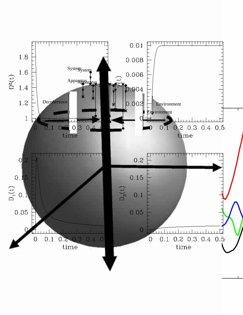
0 10 20 30time

-0.2

-0.1

0

0.1

0.2

vari

ance

dif

fere

nce

h-=0.16h-=0.064h-=0.0256

0 1 2 3 4 5 6 ln(1/ h-)

10

20

30

th-

0 10 20time

-0.1

0

0.1

0.2

vari

ance

dif

fere

nce

10-2

10-1

h-0

0.1

0.2

0.3

δ(h-)

Environment

System

Apparatus

Environment

System

Apparatus

Decoherence

Noise