and proximity data structures - cs.ubc.canando/nipsfast/slides/gray.pdf · tutorial on statistical...
TRANSCRIPT
Tutorial on Statistical N-Body Problems
and Proximity Data Structures
Alexander GraySchool of Computer ScienceCarnegie Mellon University

Outline:
1. Physics problems and methods
2. Generalized N-body problems
3. Proximity data structures
4. Dual-tree algorithms
5. Comparison
Outline:
1. Physics problems and methods
2. Generalized N-body problems
3. Proximity data structures
4. Dual-tree algorithms
5. Comparison
‘N-body problem’ of physics
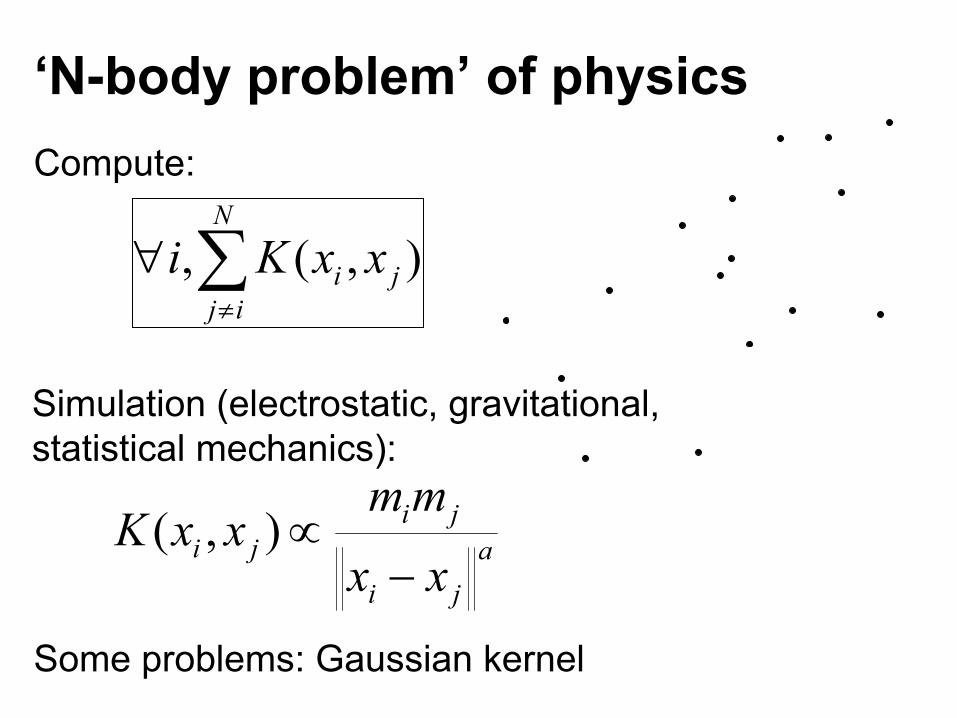
‘N-body problem’ of physics
Simulation (electrostatic, gravitational,statistical mechanics):
Compute:
aji
jiji
xx
mmxxK
−∝),(
),(, j
N
iji xxKi ∑
≠
∀
Some problems: Gaussian kernel

‘N-body problem’ of physics
Computational fluid dynamics(smoothed particle hydrodynamics):
more complicated: nonstationary,anisotropic,edge-dependent (Gray thesis 2003)
),(, j
N
iji xxKi ∑
≠
∀
Compute:
0)2(364
),( 3
32
ttt
xxK i −+−
=
22110
≥<≤<≤
ttt
22/ hxxt ji −=

‘N-body problem’ of physics
Main obstacle: )( 2NO
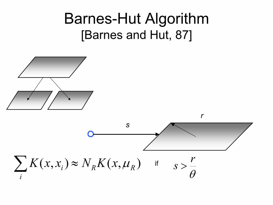
Barnes-Hut Algorithm[Barnes and Hut, 87]
∑ ≈i
RRi xKNxxK ),(),( µ if
θrs >
sr
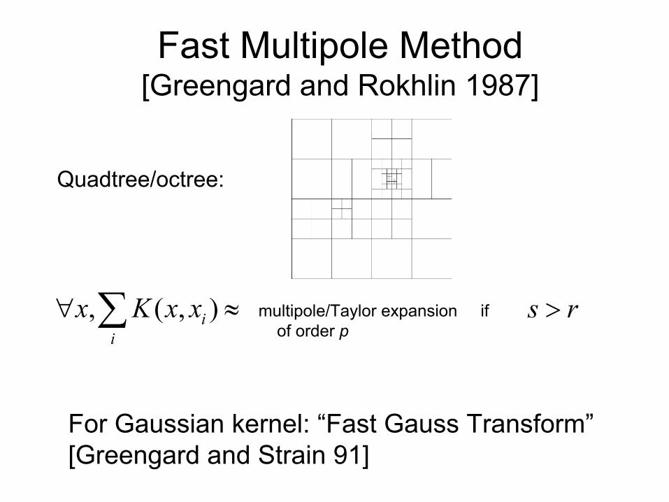
Fast Multipole Method [Greengard and Rokhlin 1987]
∑ ≈∀i
ixxKx ),(, multipole/Taylor expansion ifof order p
rs >
For Gaussian kernel: “Fast Gauss Transform”[Greengard and Strain 91]
Quadtree/octree:
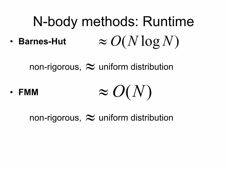
• Barnes-Hut
non-rigorous, uniform distribution
• FMM
non-rigorous, uniform distribution
N-body methods: Runtime)log( NNO≈
)(NO≈≈
≈

• Barnes-Hut
non-rigorous, uniform distribution
• FMM
non-rigorous, uniform distribution
[Callahan-Kosaraju 95]: O(N) is impossible for log-depth tree
N-body methods: Runtime)log( NNO≈
)(NO≈≈
≈

In practice…
Both are used
Often Barnes-Hut is chosen for several reasons…
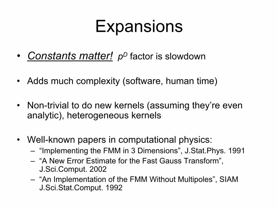
Expansions• Constants matter! pD factor is slowdown
• Adds much complexity (software, human time)
• Non-trivial to do new kernels (assuming they’re even analytic), heterogeneous kernels
• Well-known papers in computational physics: – “Implementing the FMM in 3 Dimensions”, J.Stat.Phys. 1991– “A New Error Estimate for the Fast Gauss Transform”,
J.Sci.Comput. 2002– “An Implementation of the FMM Without Multipoles”, SIAM
J.Sci.Stat.Comput. 1992

N-body methods: Adaptivity• Barnes-Hut recursive
can use any kind of tree
• FMM hand-organized control flowrequires grid structure
quad-tree/oct-tree not very adaptivekd-tree adaptiveball-tree/metric tree very adaptive

N-body methods: ComparisonBarnes-Hut FMM
runtime O(NlogN) O(N)
expansions optional required
simple,recursive? yes no
adaptive trees? yes no
error bounds? no yes

Outline:
1. Physics problems and methods
2. Generalized N-body problems
3. Proximity data structures
4. Dual-tree algorithms
5. Comparison
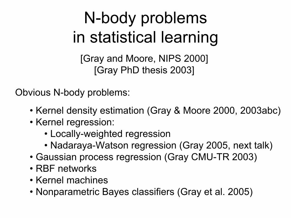
N-body problems in statistical learning
Obvious N-body problems:
[Gray and Moore, NIPS 2000][Gray PhD thesis 2003]
• Kernel density estimation (Gray & Moore 2000, 2003abc)• Kernel regression:
• Locally-weighted regression• Nadaraya-Watson regression (Gray 2005, next talk)
• Gaussian process regression (Gray CMU-TR 2003)• RBF networks • Kernel machines• Nonparametric Bayes classifiers (Gray et al. 2005)
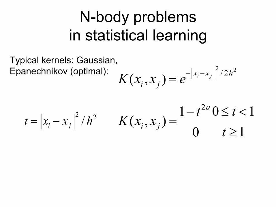
N-body problems in statistical learning
22 2/),( hxxji
jiexxK −−=
01
),(2a
jit
xxK−
=110
≥<≤
tt22
/ hxxt ji −=
Typical kernels: Gaussian, Epanechnikov (optimal):
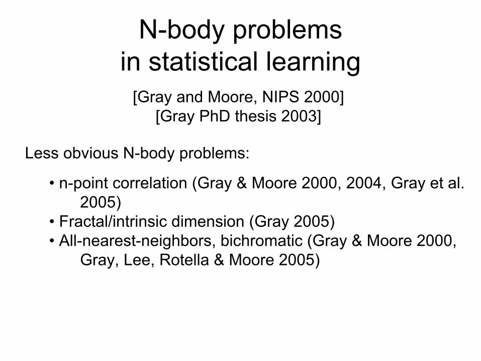
N-body problems in statistical learning
Less obvious N-body problems:
• n-point correlation (Gray & Moore 2000, 2004, Gray et al. 2005)
• Fractal/intrinsic dimension (Gray 2005)• All-nearest-neighbors, bichromatic (Gray & Moore 2000,
Gray, Lee, Rotella & Moore 2005)
[Gray and Moore, NIPS 2000][Gray PhD thesis 2003]
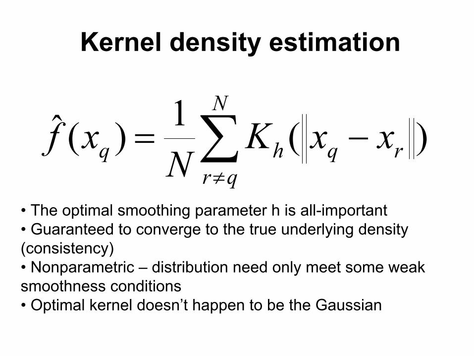
Kernel density estimation
∑≠
−=N
qrrqhq xxK
Nxf )(1)(ˆ
• The optimal smoothing parameter h is all-important• Guaranteed to converge to the true underlying density (consistency)• Nonparametric – distribution need only meet some weak smoothness conditions• Optimal kernel doesn’t happen to be the Gaussian
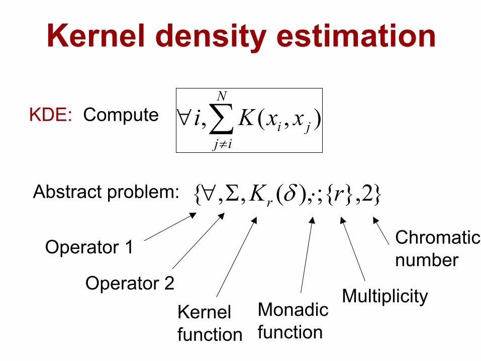
Kernel density estimation
}2},{;),(,,{ rKr ⋅Σ∀ δAbstract problem:
Operator 1
Operator 2Kernelfunction
Monadicfunction
Multiplicity
Chromaticnumber
KDE: Compute ),(, j
N
iji xxKi ∑
≠
∀

All-NN: Compute
}2;;,min,arg,{ ⋅⋅∀ δ
jijk xxi −∀ minarg,
Abstract problem:
Operator 1
Operator 2Kernelfunction
Monadicfunction
Multiplicity
Chromaticnumber
All-nearest-neighbors(bichromatic, k)
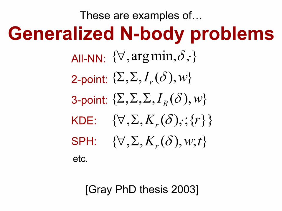
These are examples of…
Generalized N-body problemsAll-NN:
2-point:
3-point:
KDE:
SPH: };),(,,{}}{;),(,,{}),(,,,{
}),(,,{},min,arg,{
twKrKwI
wI
r
r
R
r
δδδ
δδ
Σ∀⋅Σ∀
ΣΣΣΣΣ
⋅∀
[Gray PhD thesis 2003]
etc.
Physical simulation
• High accuracy required. (e.g. 6-12 digits)
• Dimension is 1-3.
• Most problems are covered by Coulombickernel function.
Statistics/learning
• Accuracy on order of prediction accuracy required.
• Often high dimensionality.
• Test points can be different from training points.
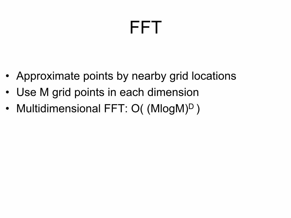
FFT
• Approximate points by nearby grid locations• Use M grid points in each dimension• Multidimensional FFT: O( (MlogM)D )

Fast Gauss Transform [Greengard and Strain 89, 91]
• Same series-expansion idea as FMM, but with Gaussian kernel
• However: no data structure• Designed for low-D setting (borrowed from physics)
• “Improved FGT” [Yang, Duraiswami 03]:– appoximation is O(Dp) instead of O(pD)– also ignore Gaussian tails beyond a threshold– choose K<√N, find K clusters; compare each cluster to
each other: O(K2)=O(N)– not a tree, just a set of clusters
Observations
• FFT: Designed for 1-D signals (borrowed from signal processing). Considered state-of-the-art in statistics.
• FGT: Designed for low-D setting (borrowed from physics). Considered state-of-the-art in computer vision.
Runtime of both depends explicitly on D.
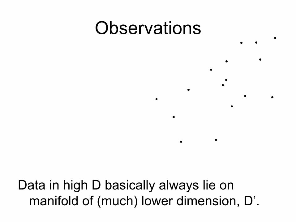
Observations
Data in high D basically always lie on manifold of (much) lower dimension, D’.
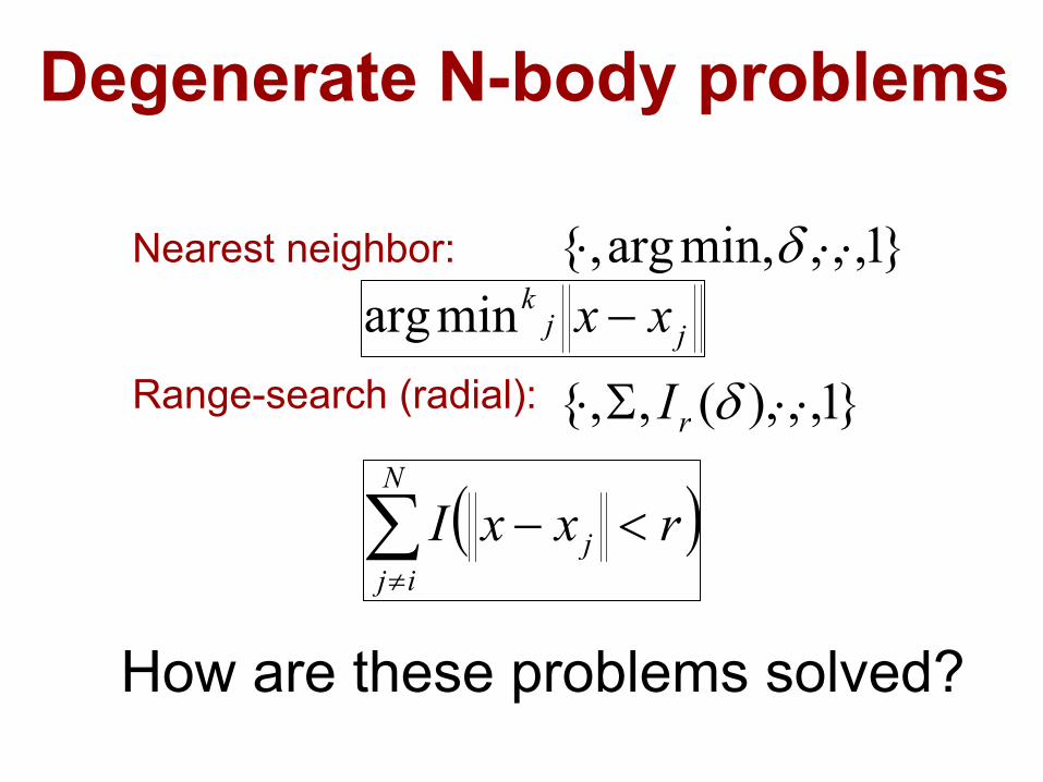
Nearest neighbor:
Range-search (radial): }1,,),(,,{
}1,,,min,arg,{
⋅⋅Σ⋅
⋅⋅⋅
δ
δ
rI
Degenerate N-body problems
How are these problems solved?
jjk xx −minarg
( )rxxI j
N
ij<−∑
≠

Outline:
1. Physics problems and methods
2. Generalized N-body problems
3. Proximity data structures
4. Dual-tree algorithms
5. Comparison

kd-trees:most widely-used space-
partitioning tree[Friedman, Bentley & Finkel 1977]
• Univariate axis-aligned splits• Split on widest dimension• O(N log N) to build, O(N) space

A kd-tree: level 1
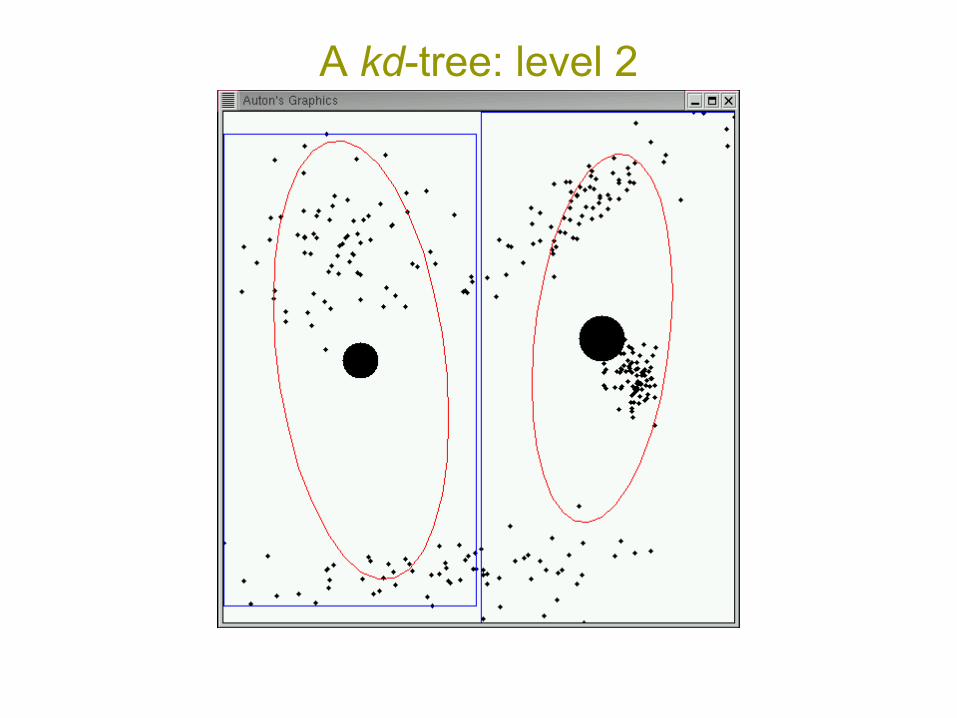
A kd-tree: level 2

A kd-tree: level 3

A kd-tree: level 4
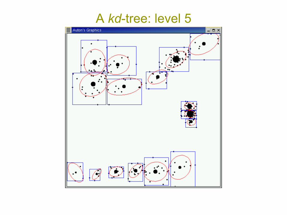
A kd-tree: level 5
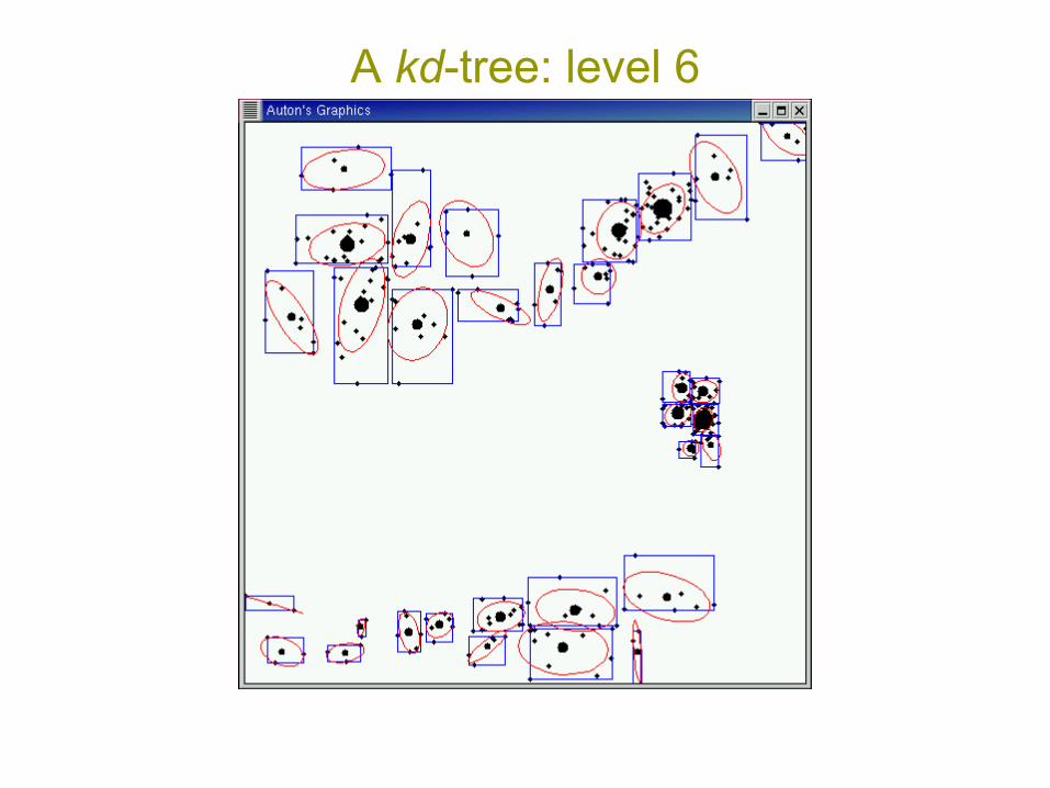
A kd-tree: level 6
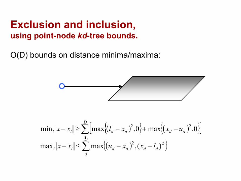
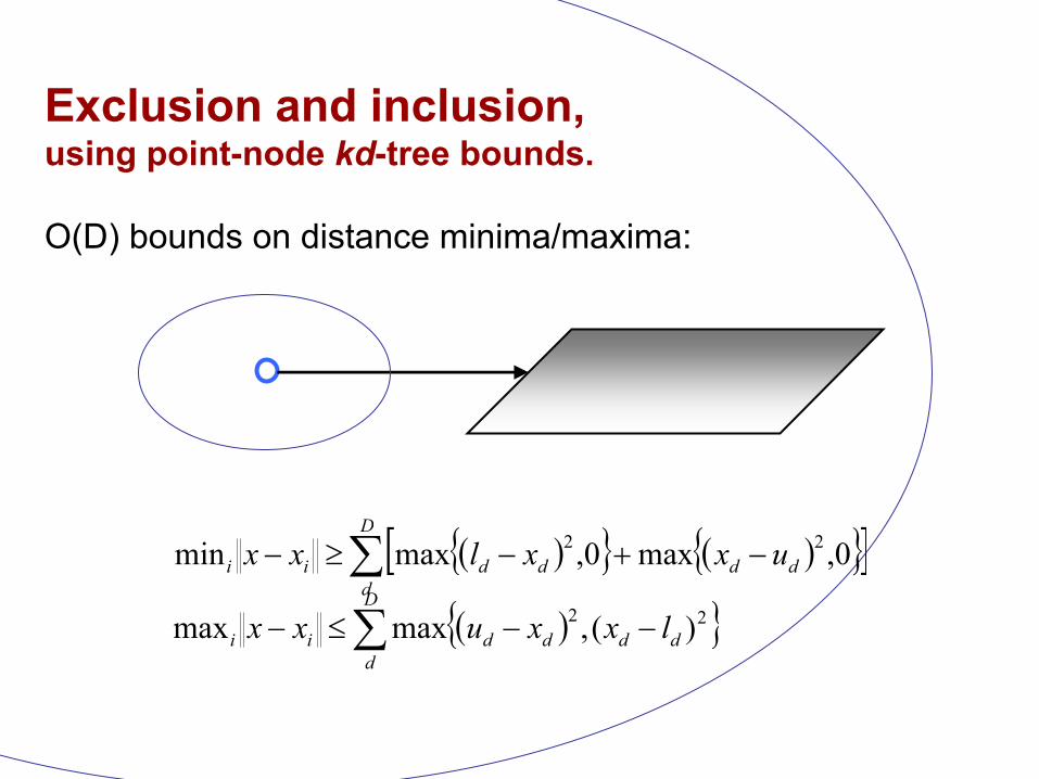
Exclusion and inclusion,using point-node kd-tree bounds.
O(D) bounds on distance minima/maxima:
( ){ } ( ){ }[ ]∑ −+−≥−D
dddddii uxxlxx 0,max0,maxmin 22
( ){ }∑ −−≤−D
dddddii lxxuxx 22 )(,maxmax
Exclusion and inclusion,using point-node kd-tree bounds.
O(D) bounds on distance minima/maxima:
( ){ } ( ){ }[ ]∑ −+−≥−D
dddddii uxxlxx 0,max0,maxmin 22
( ){ }∑ −−≤−D
dddddii lxxuxx 22 )(,maxmax
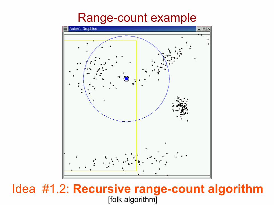
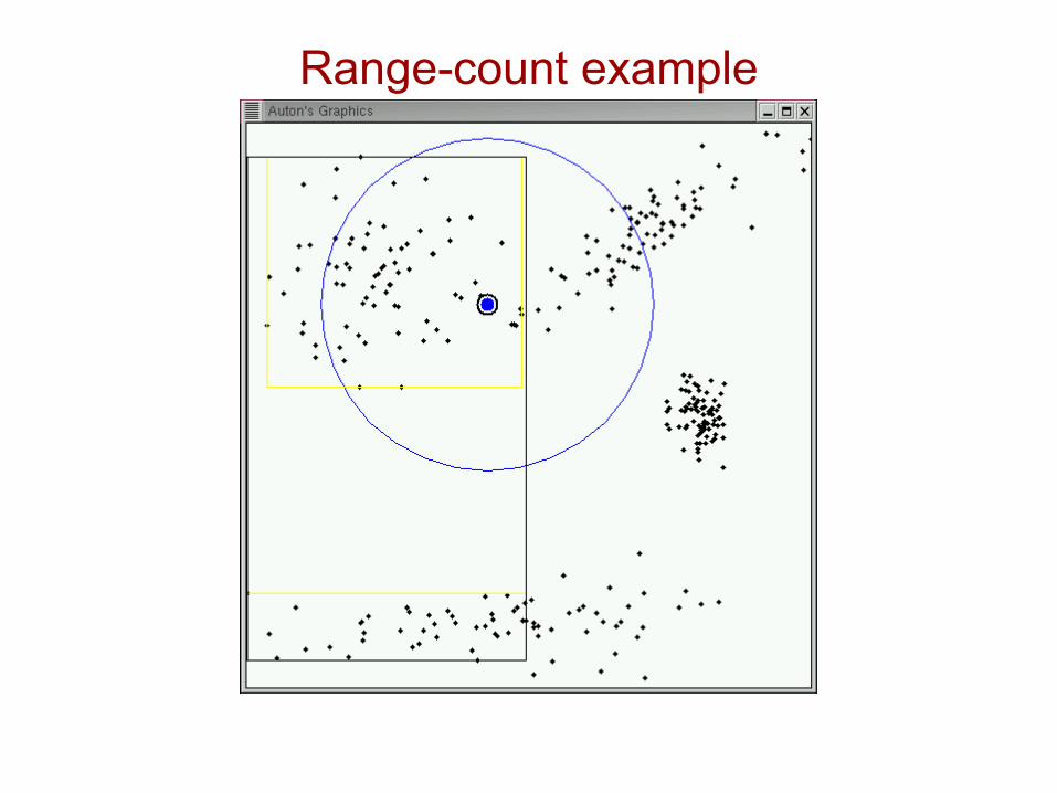
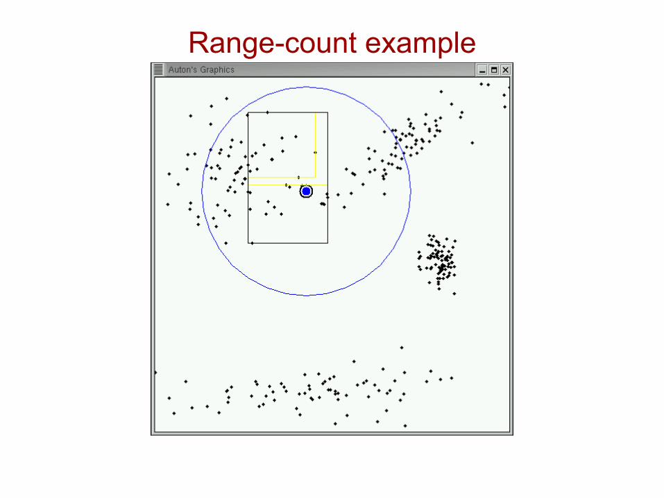
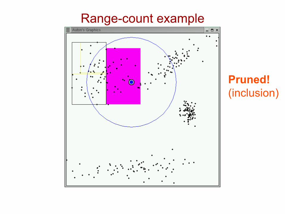
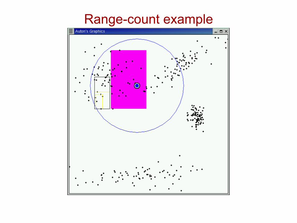
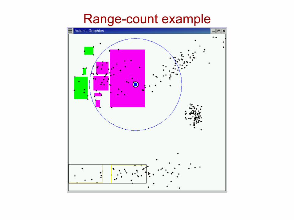
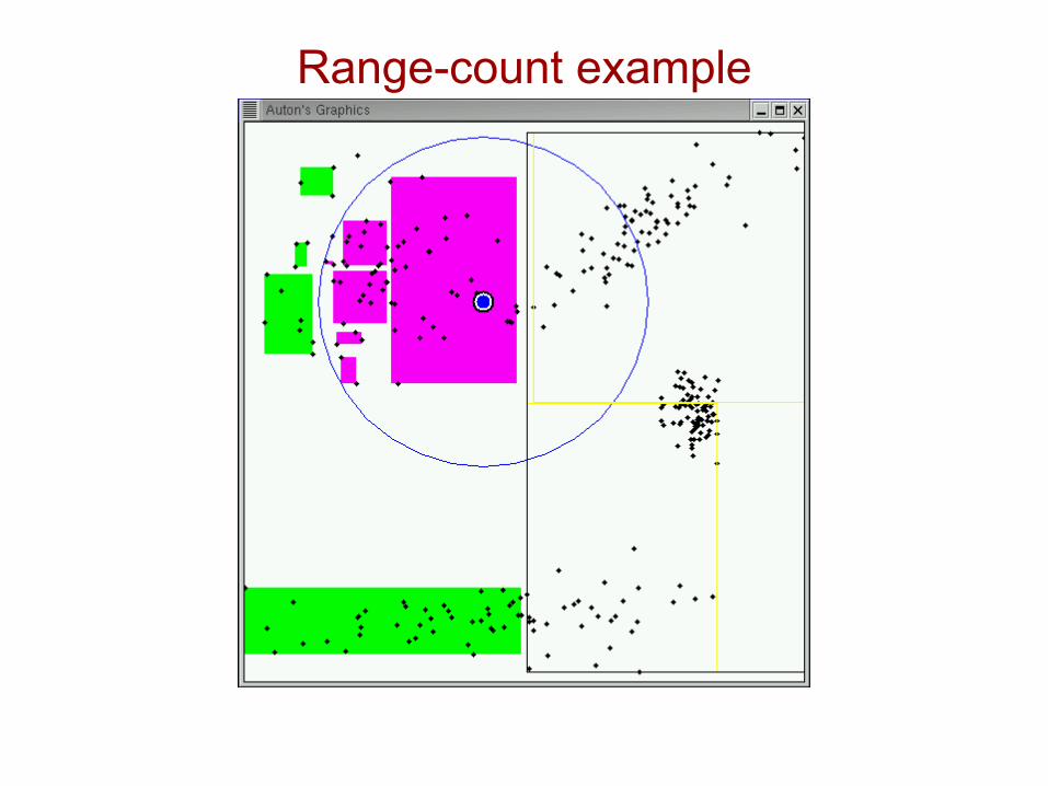
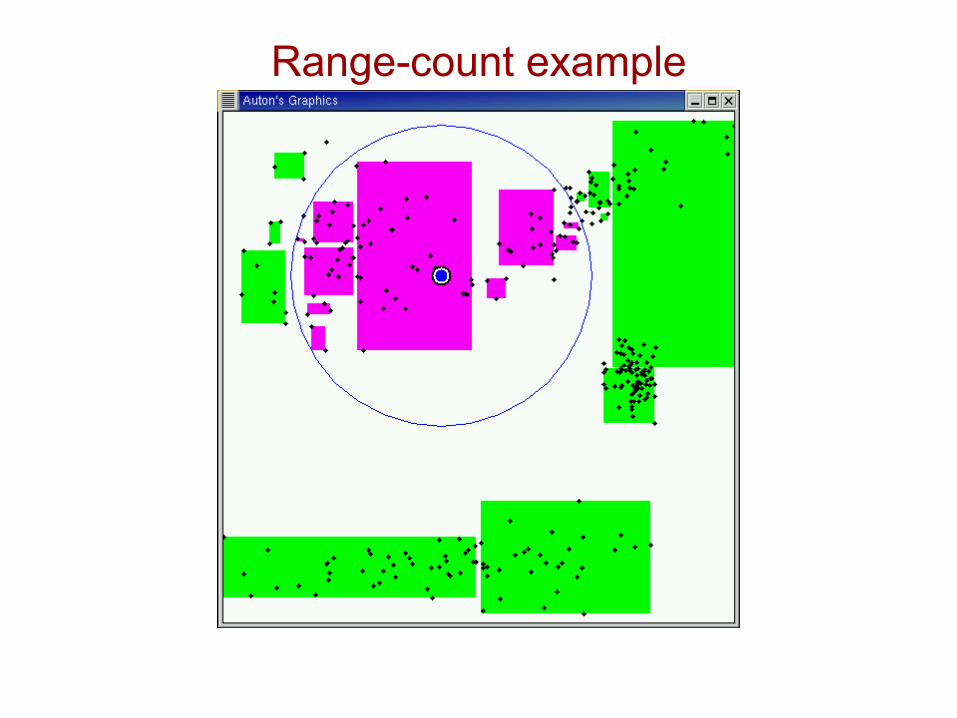
Range-count example
Idea #1.2: Recursive range-count algorithm[folk algorithm]
Range-count example

Range-count example
Range-count example
Range-count example
Pruned!(inclusion)

Range-count example
Range-count example

Range-count example

Range-count example

Range-count example

Range-count example

Range-count example

Range-count example
Pruned!(exclusion)
Range-count example
Range-count example
Range-count example
What’s the best data structurefor proximity problems?
• There are hundreds of papers which have proposed nearest-neighbor data structures (maybe even thousands)
• Empirical comparisons are usually to one or two strawman methods
Nobody really knows how things compare

The Proximity Project[Gray, Lee, Rotella, Moore 2005]
Careful agostic empirical comparison, open source15 datasets, dimension 2-1MThe most well-known methods from 1972-2004
• Exact NN: 15 methods• All-NN, mono & bichromatic: 3 methods• Approximate NN: 10 methods• Point location: 3 methods• (NN classification: 3 methods)• (Radial range search: 3 methods)

…and the overall winner is?(exact NN, high-D)
Ball-trees, basically – though there is high variance and dataset dependence
• Auton ball-trees III [Omohundro 91],[Uhlmann 91], [Moore 99]
• Cover-trees [Alina B.,Kakade,Langford 04]
• Crust-trees [Yianilos 95],[Gray,Lee,Rotella,Moore 2005]
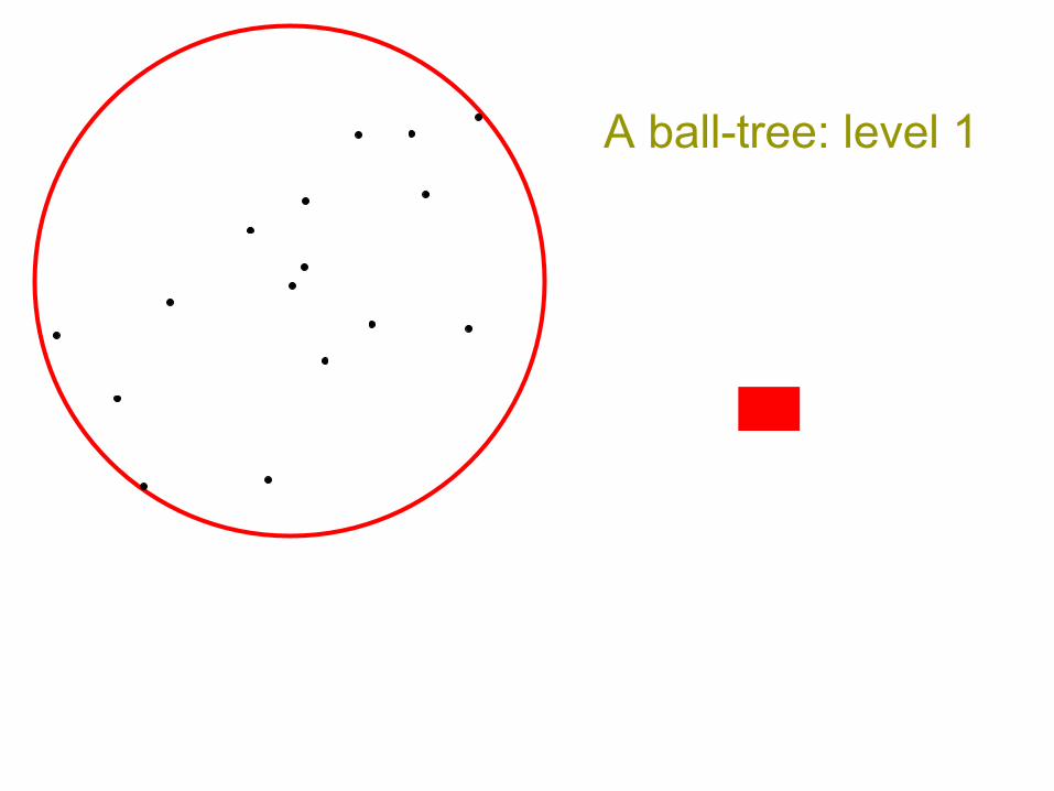
A ball-tree: level 1

A ball-tree: level 2

A ball-tree: level 3

A ball-tree: level 4

A ball-tree: level 5

Anchors Hierarchy [Moore 99]
• ‘Middle-out’ construction• Uses farthest-point method [Gonzalez 85] to
find sqrt(N) clusters – this is the middle• Bottom-up construction to get the top• Top-down division to get the bottom• Smart pruning throughout to make it fast• (NlogN), very fast in practice
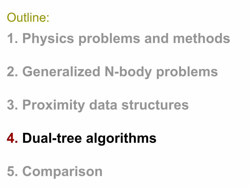
Outline:
1. Physics problems and methods
2. Generalized N-body problems
3. Proximity data structures
4. Dual-tree algorithms
5. Comparison
Questions
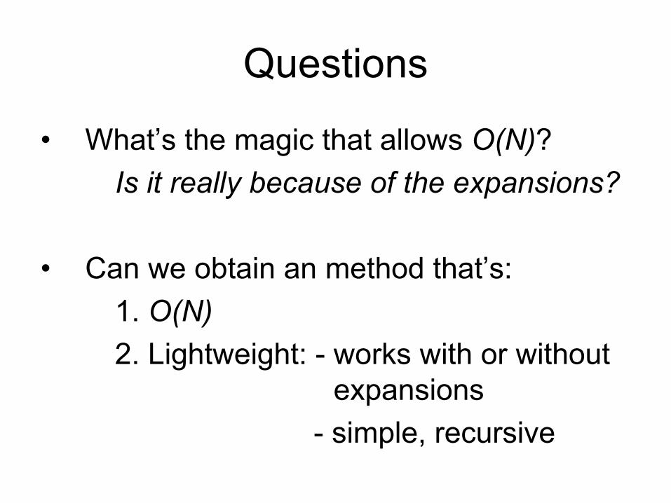
• What’s the magic that allows O(N)?Is it really because of the expansions?
• Can we obtain an method that’s:1. O(N)2. Lightweight: - works with or without
..............................expansions- simple, recursive
New algorithm
• Use an adaptive tree (kd-tree or ball-tree)
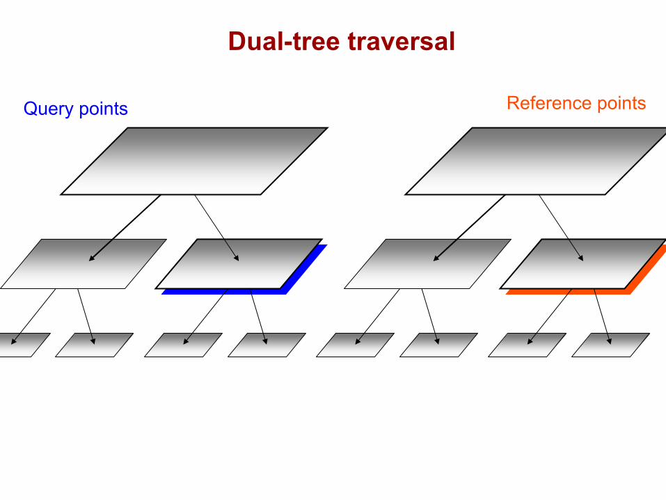
• Dual-tree recursion
• Finite-difference approximation
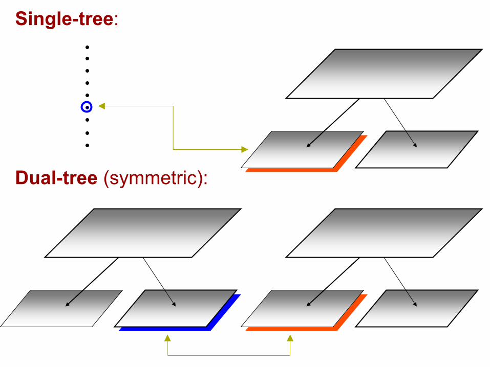
Single-tree:
Dual-tree (symmetric):
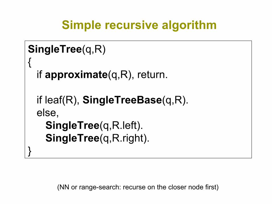
Simple recursive algorithm
SingleTree(q,R){
if approximate(q,R), return.
if leaf(R), SingleTreeBase(q,R).else,
SingleTree(q,R.left).SingleTree(q,R.right).
}
(NN or range-search: recurse on the closer node first)
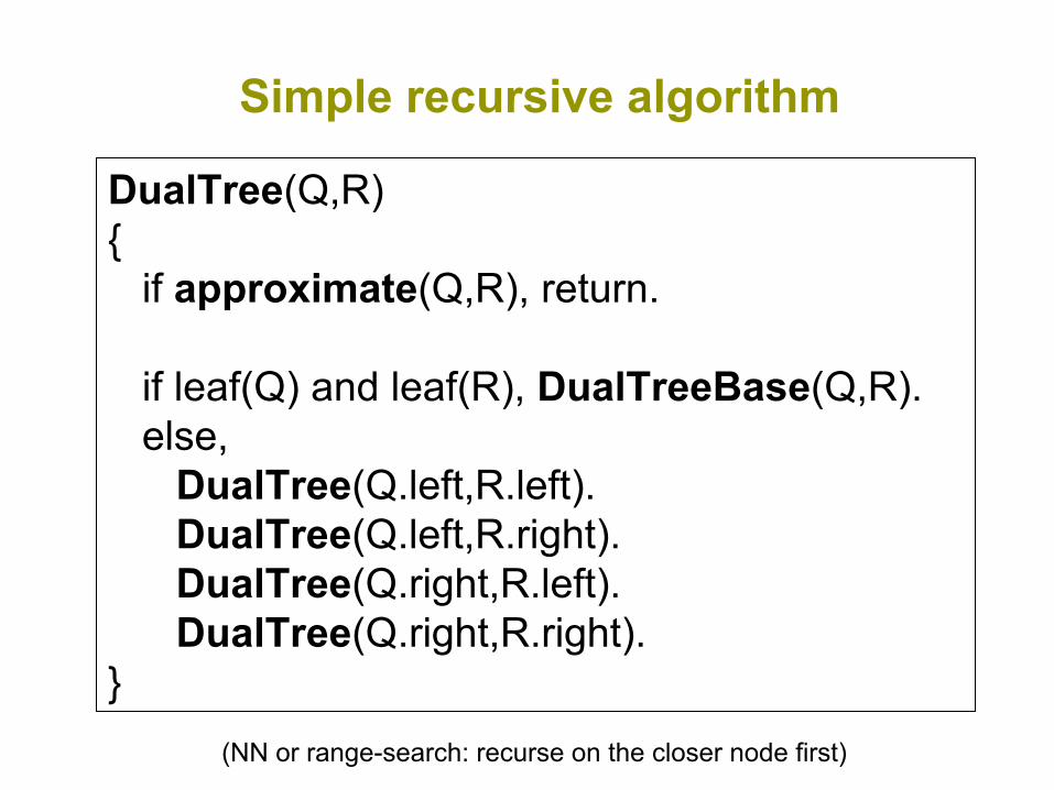
Simple recursive algorithm
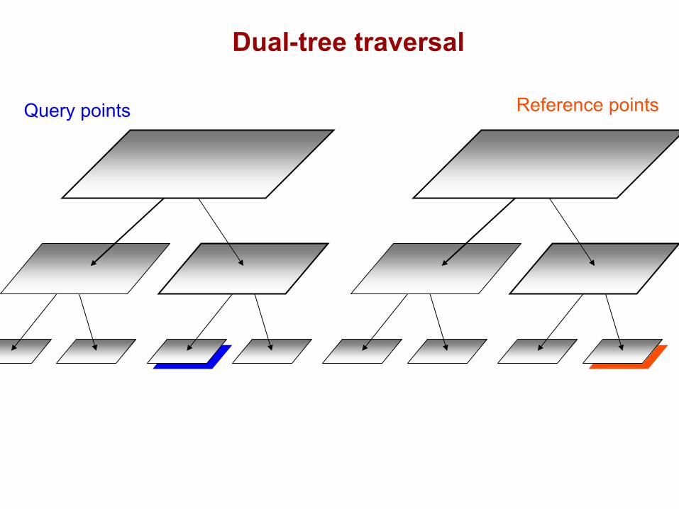
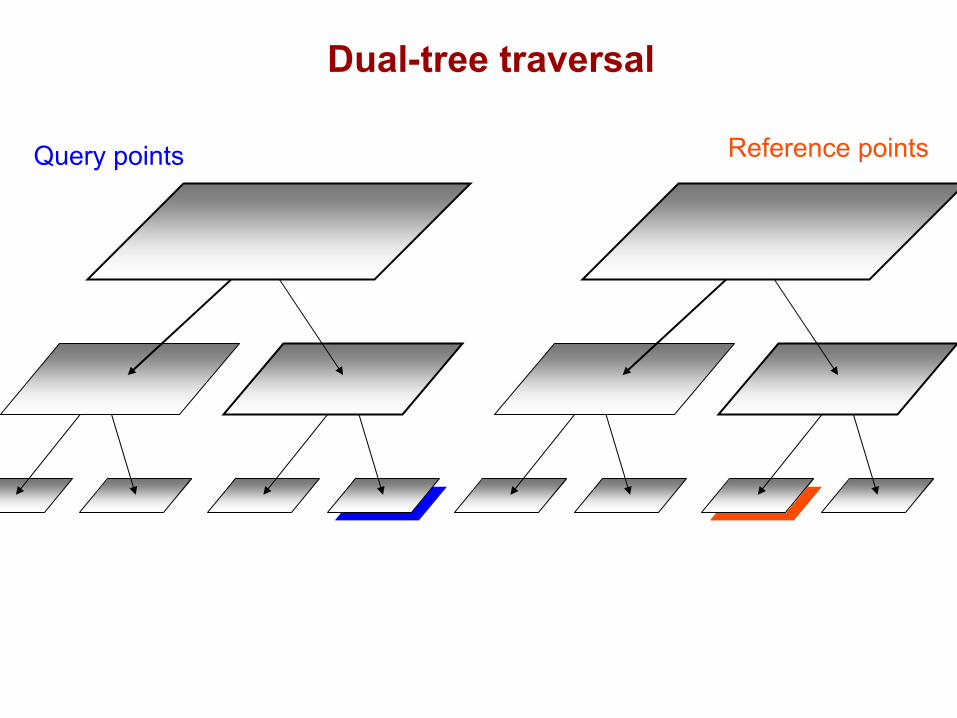
DualTree(Q,R){
if approximate(Q,R), return.
if leaf(Q) and leaf(R), DualTreeBase(Q,R).else,
DualTree(Q.left,R.left).DualTree(Q.left,R.right).DualTree(Q.right,R.left).DualTree(Q.right,R.right).
}(NN or range-search: recurse on the closer node first)
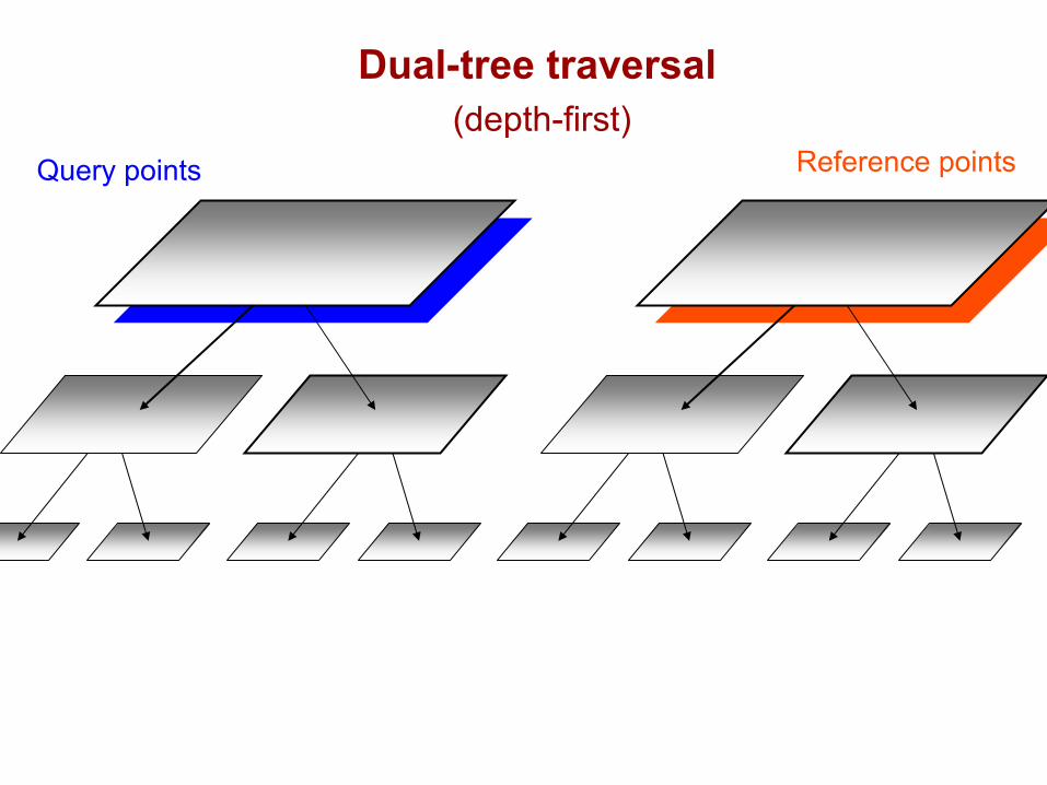
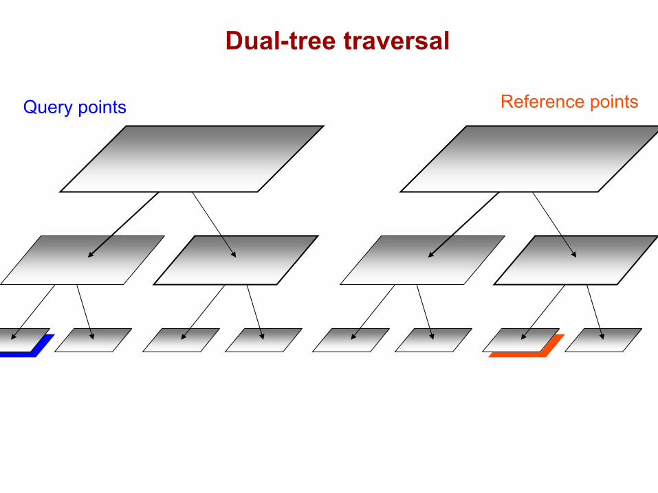
Query points Reference points
Dual-tree traversal(depth-first)

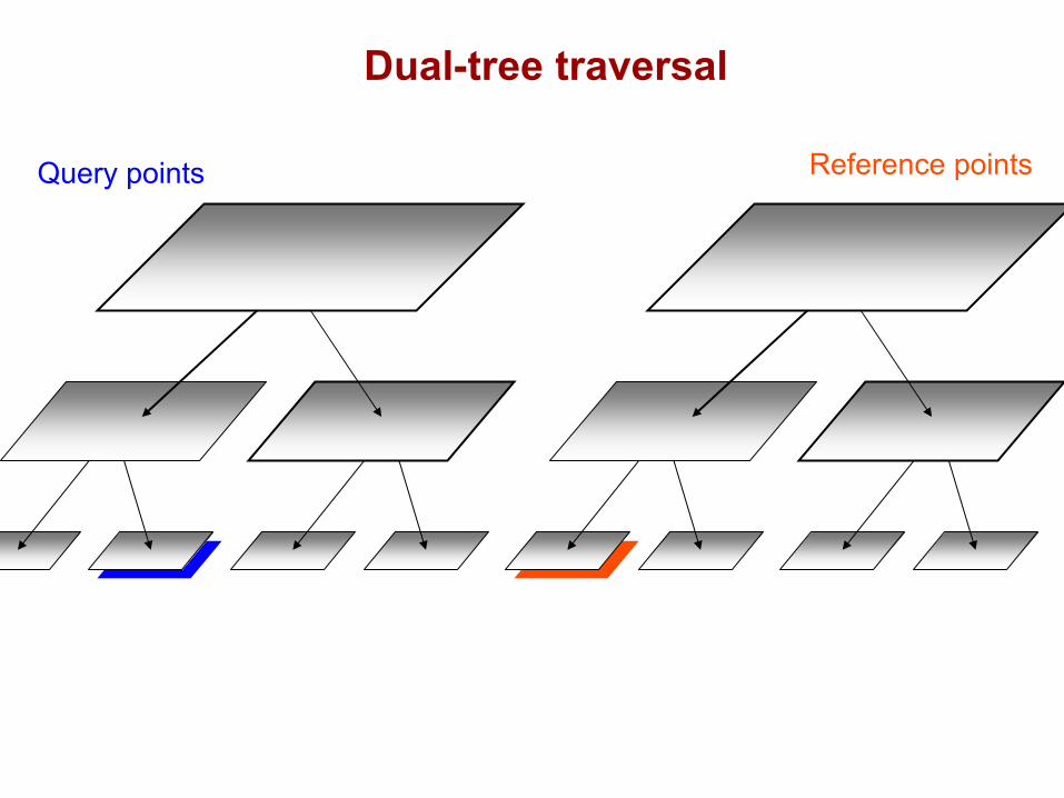
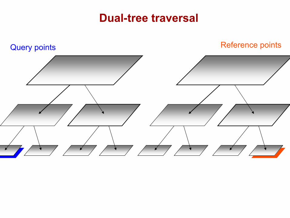
Query points Reference points
Dual-tree traversal

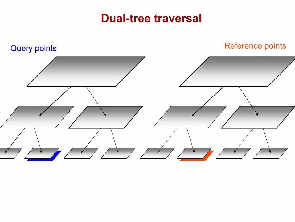
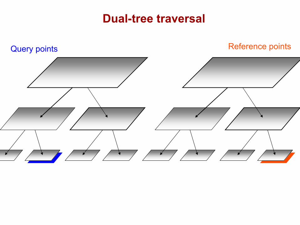
Query points Reference points
Dual-tree traversal

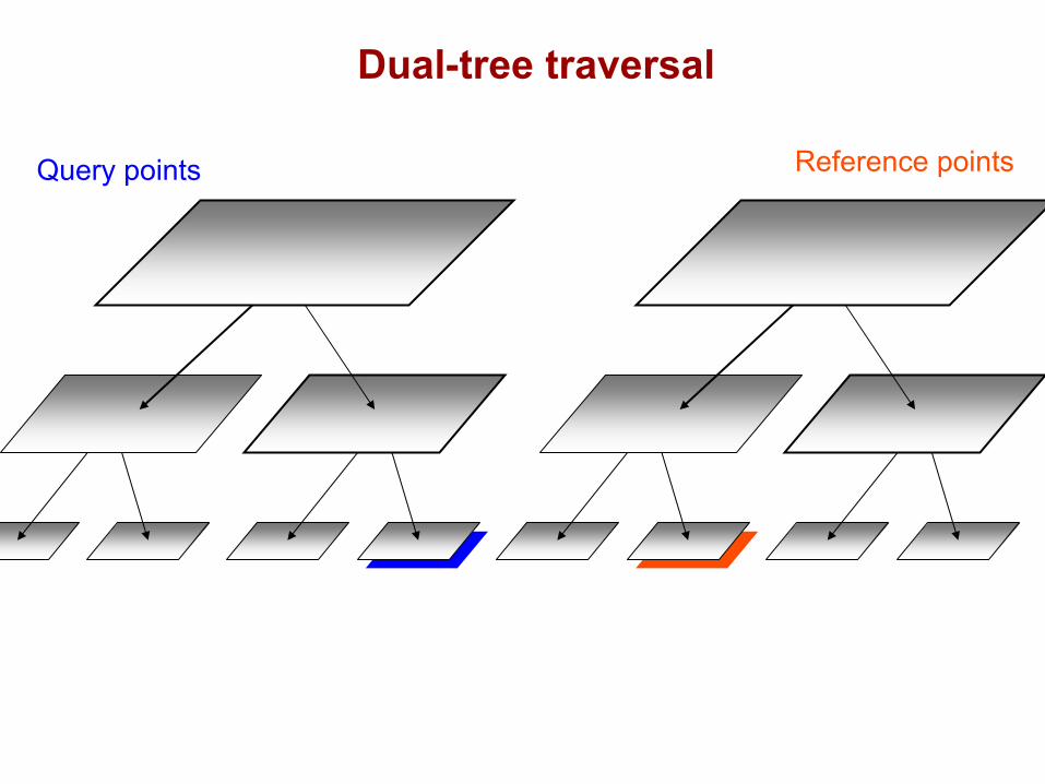
Query points Reference points
Dual-tree traversal
Query points Reference points
Dual-tree traversal
Query points Reference points
Dual-tree traversal

Query points Reference points
Dual-tree traversal
Query points Reference points
Dual-tree traversal
Query points Reference points
Dual-tree traversal

Query points Reference points
Dual-tree traversal
Query points Reference points
Dual-tree traversal

Query points Reference points
Dual-tree traversal

Query points Reference points
Dual-tree traversal

Query points Reference points
Dual-tree traversal

Query points Reference points
Dual-tree traversal
Query points Reference points
Dual-tree traversal
Query points Reference points
Dual-tree traversal

Query points Reference points
Dual-tree traversal
Query points Reference points
Dual-tree traversal
Query points Reference points
Dual-tree traversal

Query points Reference points
Dual-tree traversal
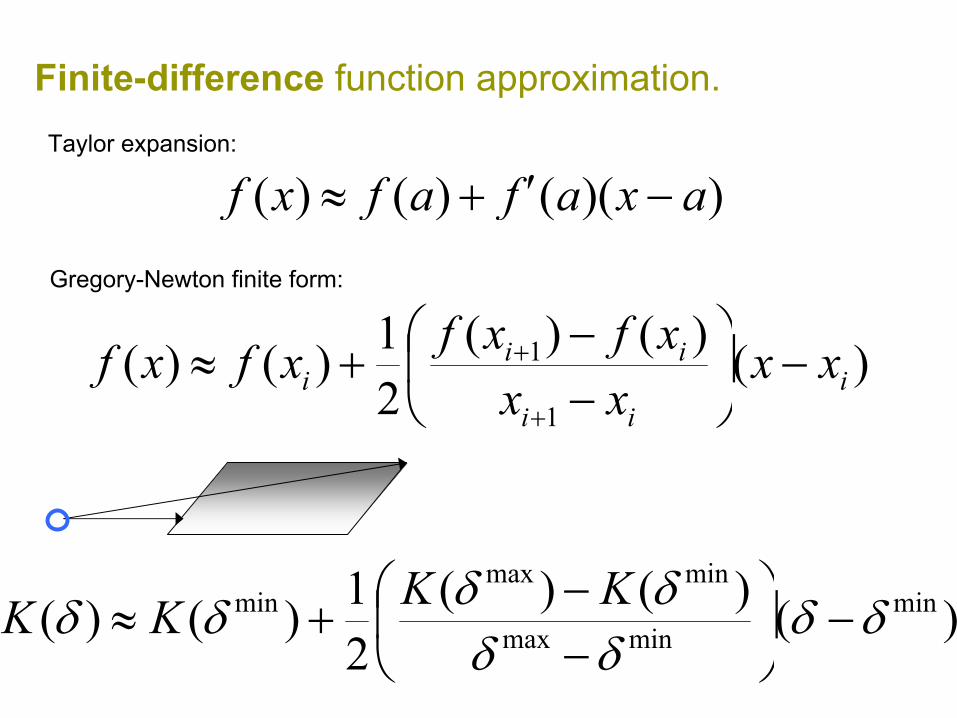
Finite-difference function approximation.
)()()(21)()(
1
1i
ii
iii xx
xxxfxfxfxf −
−−+≈
+
+
)()()(21)()( min
minmax
minmaxmin δδ
δδδδδδ −
−−+≈ KKKK
))(()()( axafafxf −′+≈Taylor expansion:
Gregory-Newton finite form:
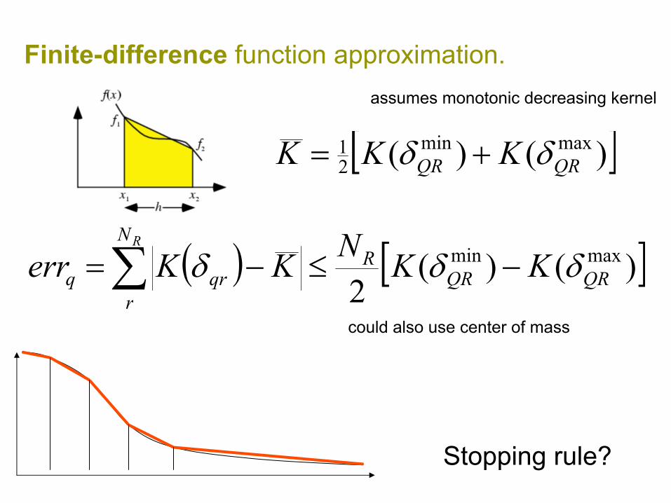
Finite-difference function approximation.
( ) [ ])()(2
maxminQRQR
RN
rqrq KKNKKerr
R
δδδ −≤−=∑
[ ])()( maxmin21
QRQR KKK δδ +=
assumes monotonic decreasing kernel
Stopping rule?
could also use center of mass

Simple approximation method
approximate(Q,R){
if
incorporate(dl, du).}
))(),(max(min RdiamQdiam⋅≥τδ
).(),( minmax δδ KNduKNdl RR ==
trivial to change kernelhard error bounds

Big issue in practice…
Tweak parameters
Case 1 – algorithm gives no error boundsCase 2 – algorithm gives hard error bounds: must run it many timesCase 3 – algorithm automatically achives your error tolerance

Automatic approximation method
approximate(Q,R){
if
incorporate(dl, du). return.}
)()()( min2
maxmin QKK N φδδ ε≤−
).(),( minmax δδ KNduKNdl RR ==
just set error tolerance, no tweak parametershard error bounds
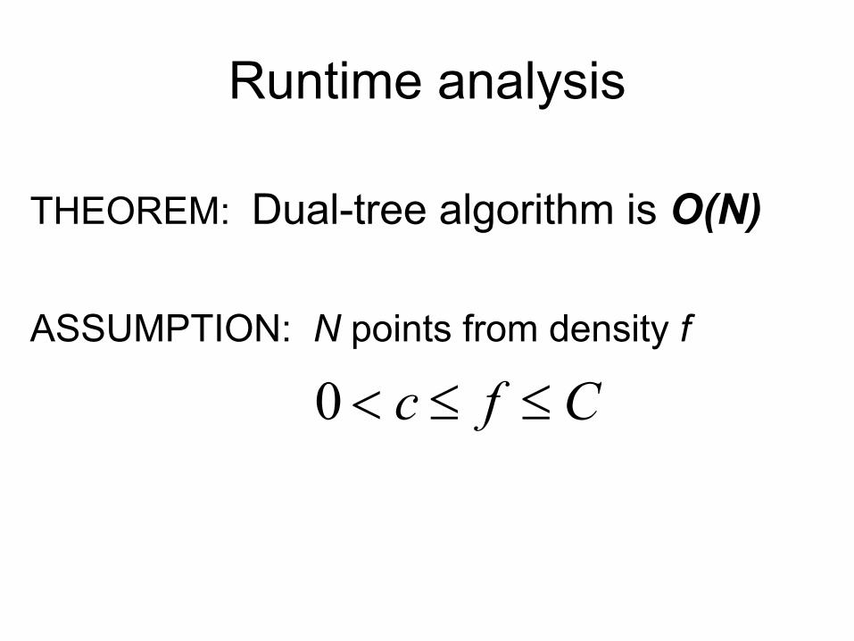
Runtime analysis
THEOREM: Dual-tree algorithm is O(N)
ASSUMPTION: N points from density f
Cfc ≤≤<0
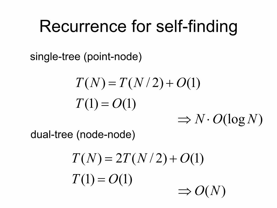
Recurrence for self-finding
)(logNON ⋅⇒)1()1(
)1()2/()(OT
ONTNT=
+=
)1()1()1()2/(2)(
OTONTNT
=+=
single-tree (point-node)
dual-tree (node-node)
)(NO⇒
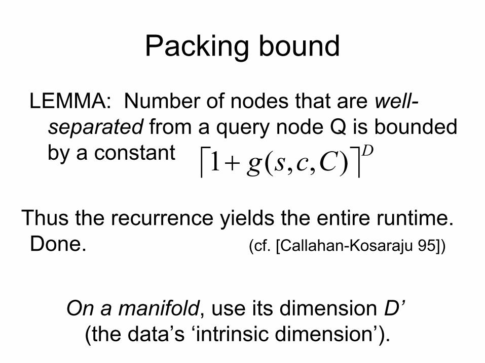
Packing bound
LEMMA: Number of nodes that are well-separated from a query node Q is bounded by a constant
DCcsg ),,(1+
Thus the recurrence yields the entire runtime.Done. (cf. [Callahan-Kosaraju 95])
On a manifold, use its dimension D’(the data’s ‘intrinsic dimension’).
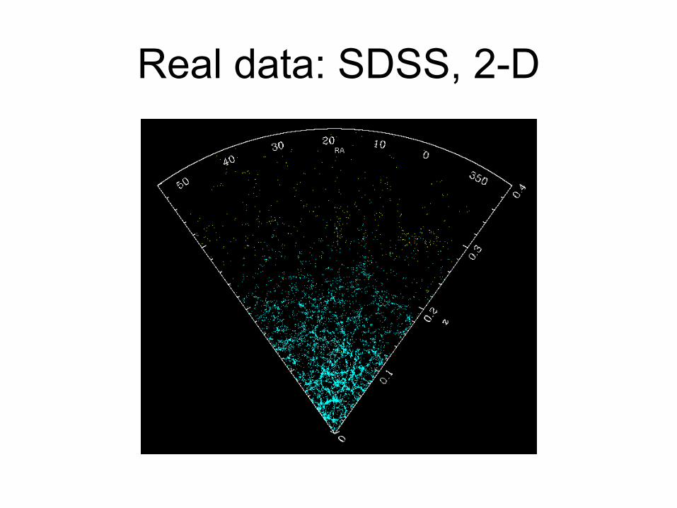
Real data: SDSS, 2-D
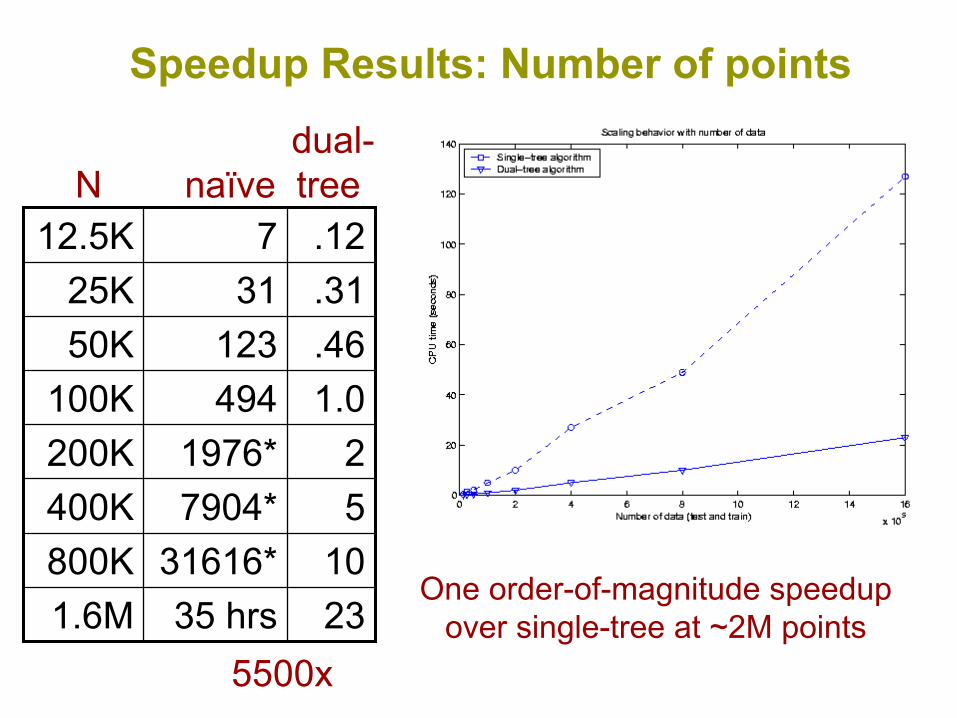
Speedup Results: Number of points
One order-of-magnitude speedupover single-tree at ~2M points2335 hrs1.6M
1031616*800K57904*400K21976*200K
1.0494100K.4612350K.313125K.12712.5K
dual-N naïve tree
5500x

Speedup Results: Different kernels
51231.6M2210800K115400K
52200K21.0100K
1.1.4650K.70.3125K.32.1212.5K
N Epan. Gauss.
Epanechnikov: 10-6 relative error
Gaussian: 10-3 relative error

Speedup Results: Dimensionality
51231.6M2210800K115400K
52200K21.0100K
1.1.4650K.70.3125K.32.1212.5K
N Epan. Gauss.

Speedup Results: Different datasets
Name N D Time (sec)
923MPSF2d
2478410KMNIST
838136KCovType
105103KBio5
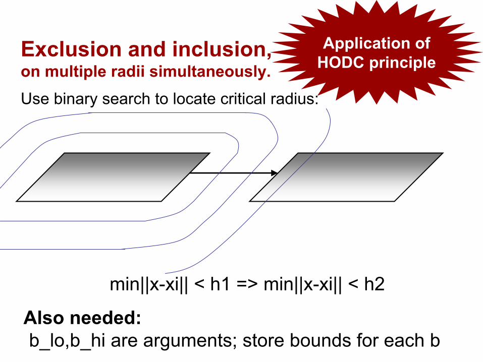
Exclusion and inclusion,on multiple radii simultaneously.Use binary search to locate critical radius:
min||x-xi|| < h1 => min||x-xi|| < h2
Also needed:b_lo,b_hi are arguments; store bounds for each b
Application ofHODC principle

Speedup Results
One order-of-magnitude speedupover single-radius at ~10,000 radii
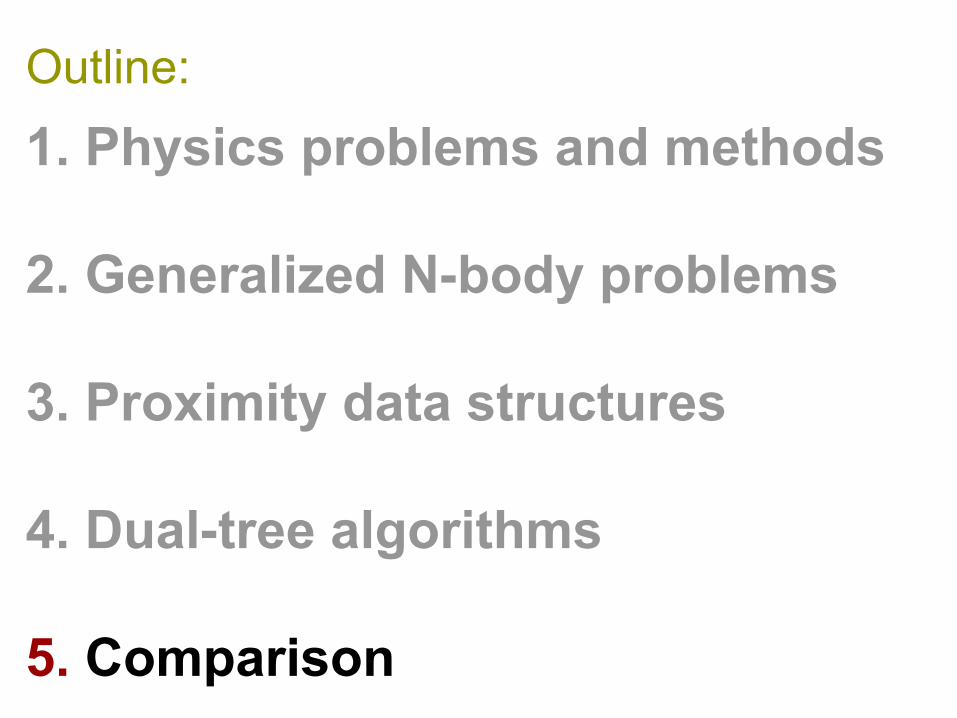
Outline:
1. Physics problems and methods
2. Generalized N-body problems
3. Proximity data structures
4. Dual-tree algorithms
5. Comparison

Experiments
• Optimal bandwidth h* found by LSCV• Error relative to truth: maxerr=max |est – true| / true• Only require that 95% of points meet this tolerance• Measure CPU time given this error level• Note that these are small datasets for manageability• Methods compared:
– FFT– IFGT– Dual-tree (Gaussian)– Dual-tree (Epanechnikov)
Experiments: tweak parameters
• FFT tweak parameter M: M=16, double until error satisfied
• IFGT tweak parameters K, rx, ry, p: 1) K=√N, get rx, ry=rx; 2) K=10√N, get rx, ry=16 and doubled until error satisfied; hand-tune p for dataset: {8,8,5,3,2}
• Dualtree tweak parameter tau: tau=maxerr, double until error satisfied
• Dualtree auto: just give it maxerr

colors (N=50k, D=2)
58.26.7 (6.7*)6.5 (6.7*)6.2 (6.7*)Dualtree(Epanech.)
-24.8 (117.2*)
18.7 (89.8*)
12.2 (65.1*)
Dualtree(Gaussian)
->Exhaust.>Exhaust.1.7IFGT
->Exhaust.2.90.1FFT
329.7[111.0]
---Exhaustive
Exact1%10%50%
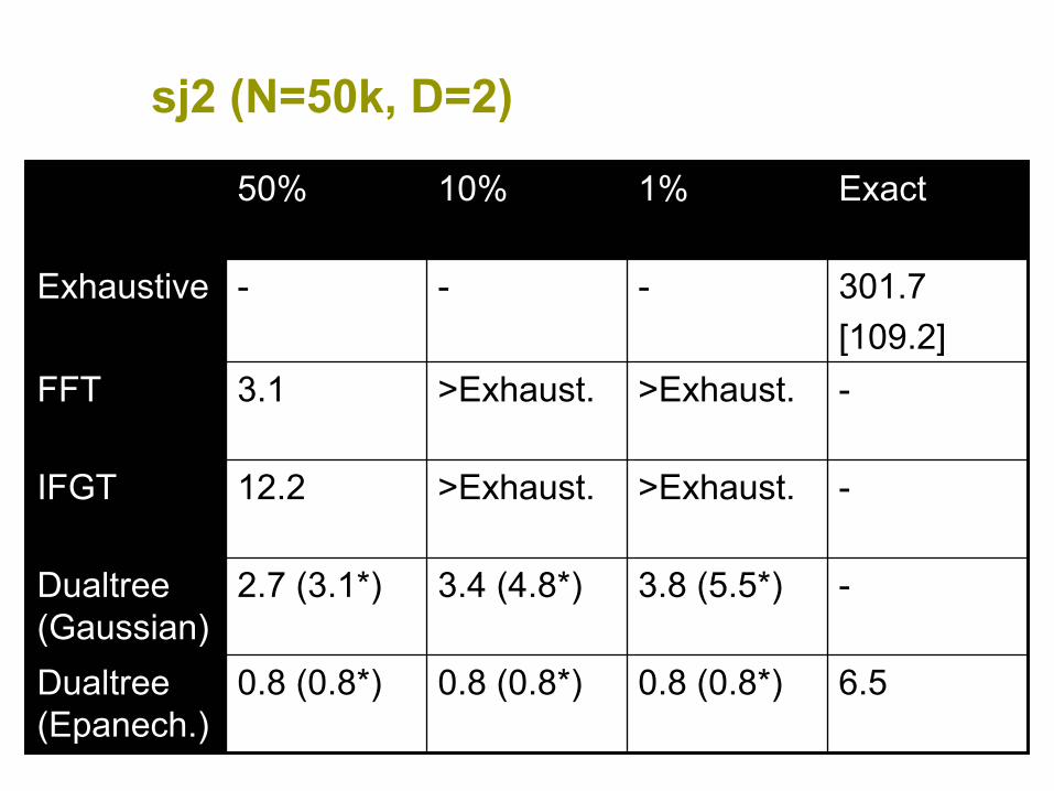
sj2 (N=50k, D=2)
6.50.8 (0.8*)0.8 (0.8*)0.8 (0.8*)Dualtree(Epanech.)
-3.8 (5.5*)3.4 (4.8*)2.7 (3.1*)Dualtree(Gaussian)
->Exhaust.>Exhaust.12.2IFGT
->Exhaust.>Exhaust.3.1FFT
301.7[109.2]
---Exhaustive
Exact1%10%50%

bio5 (N=100k, D=5)
408.928.4 (28.4*)
28.4 (28.4*)
27.0 (28.2*)
Dualtree(Epanech.)
-87.5 (128.7*)
79.6 (111.8*)
72.2 (98.8*)
Dualtree(Gaussian)
->Exhaust.>Exhaust.>Exhaust.IFGT
->Exhaust.>Exhaust.>Exhaust.FFT
1966.3[1074.9]
---Exhaustive
Exact1%10%50%

corel (N=38k, D=32)
261.610.1 (10.1*)
10.1 (10.1*)
10.0 (10.0*)
Dualtree(Epanech.)
-162.2 (167.6*)
159.9 (163*)
155.9 (159.7*)
Dualtree(Gaussian)
->Exhaust.>Exhaust.>Exhaust.IFGT
->Exhaust.>Exhaust.>Exhaust.FFT
710.2[558.7]
---Exhaustive
Exact1%10%50%
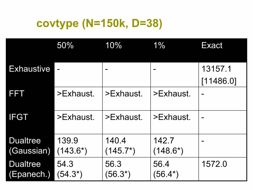
covtype (N=150k, D=38)
1572.056.4 (56.4*)
56.3 (56.3*)
54.3 (54.3*)
Dualtree(Epanech.)
-142.7 (148.6*)
140.4 (145.7*)
139.9 (143.6*)
Dualtree(Gaussian)
->Exhaust.>Exhaust.>Exhaust.IFGT
->Exhaust.>Exhaust.>Exhaust.FFT
13157.1[11486.0]
---Exhaustive
Exact1%10%50%
Myths
Multipole expansions are needed to:1. Achieve O(N) 2. Achieve high accuracy3. Have hard error bounds
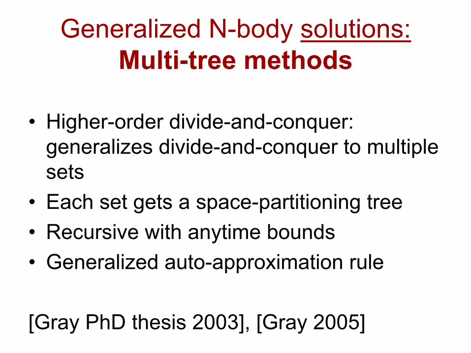
• Higher-order divide-and-conquer: generalizes divide-and-conquer to multiple sets
• Each set gets a space-partitioning tree• Recursive with anytime bounds• Generalized auto-approximation rule
[Gray PhD thesis 2003], [Gray 2005]
Generalized N-body solutions:Multi-tree methods
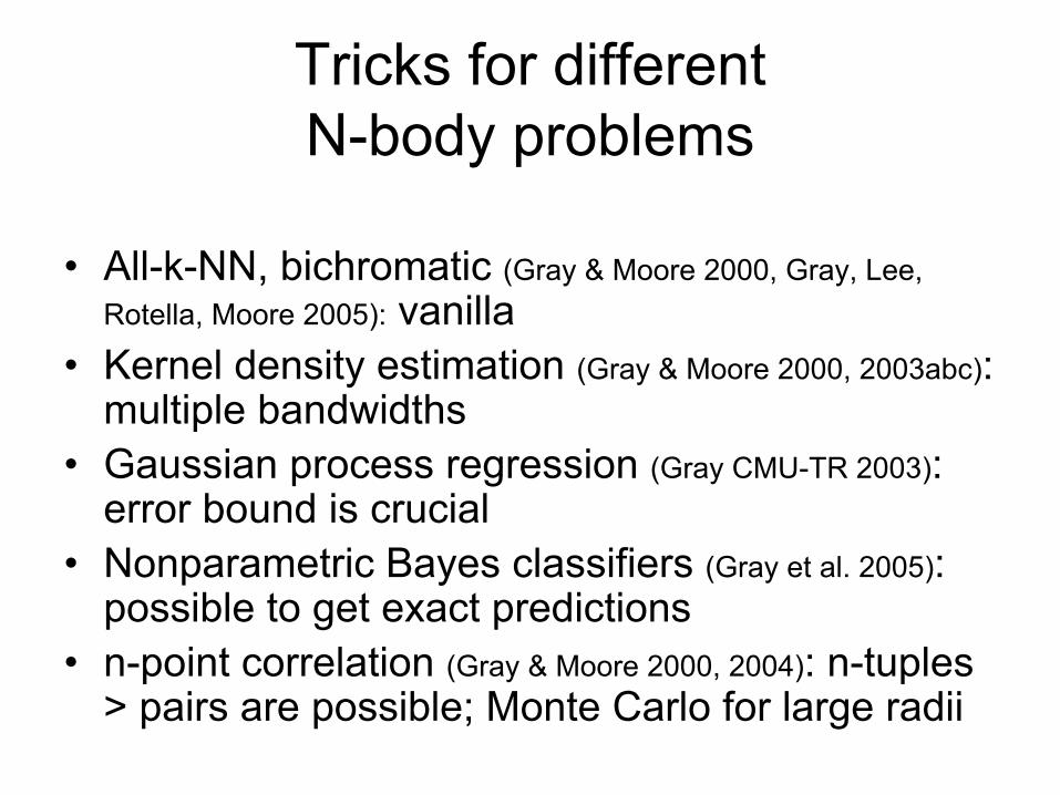
• All-k-NN, bichromatic (Gray & Moore 2000, Gray, Lee, Rotella, Moore 2005): vanilla
• Kernel density estimation (Gray & Moore 2000, 2003abc): multiple bandwidths
• Gaussian process regression (Gray CMU-TR 2003): error bound is crucial
• Nonparametric Bayes classifiers (Gray et al. 2005): possible to get exact predictions
• n-point correlation (Gray & Moore 2000, 2004): n-tuples> pairs are possible; Monte Carlo for large radii
Tricks for different N-body problems
Discussion• Related ideas: WSPD, spatial join, Appel’s
algorithm
• FGT with a tree: coming soon
• Auto-approx FGT with a tree: unclear how to do this
Summary• Statistics problems have their own properties, and benefit
from a fundamentally rethought methodology
• O(N) can be achieved without multipole expansions; via geometry
• Hard anytime error bounds are given to the user
• Tweak parameters should and can be eliminated
• Very general methodology
• Future work: tons (even in physics)Looking for comments and collaborators! [email protected]

THE END

Simple recursive algorithm
DualTree(Q,R){
if approximate(Q,R), return.
if leaf(Q) and leaf(R), DualTreeBase(Q,R).else,
DualTree(Q.left,closer-of(R.left,R.right)).DualTree(Q.left,farther-of(R.left,R.right)).DualTree(Q.right,closer-of(R.left,R.right)).DualTree(Q.right,farther-of(R.left,R.right)).
}(Actually, recurse on the closer node first)
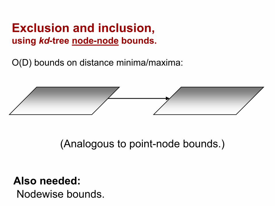
Exclusion and inclusion,using kd-tree node-node bounds.
O(D) bounds on distance minima/maxima:
(Analogous to point-node bounds.)
Also needed:Nodewise bounds.
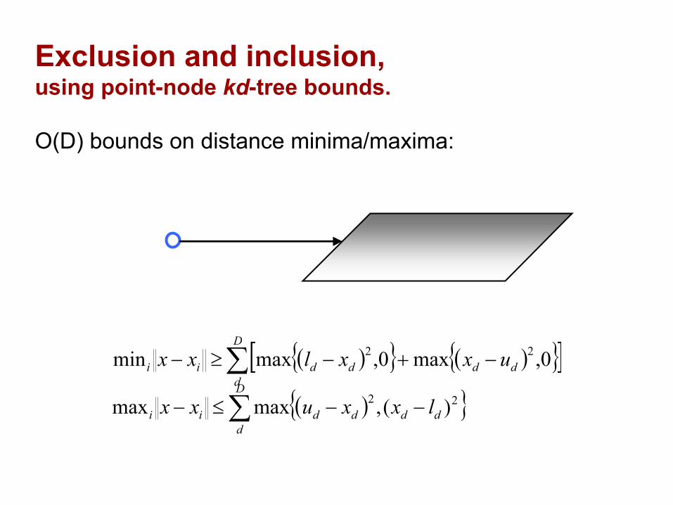
Exclusion and inclusion,using point-node kd-tree bounds.
O(D) bounds on distance minima/maxima:
( ){ } ( ){ }[ ]∑ −+−≥−D
dddddii uxxlxx 0,max0,maxmin 22
( ){ }∑ −−≤−D
dddddii lxxuxx 22 )(,maxmax