and 10.0 s - david m. boore

Ground-Motion Prediction Equationsfor the Average Horizontal Componentof PGA, PGV, and 5%-Damped PSAat Spectral Periods between 0.01 sand 10.0 s

David M. Boorea) and Gail M. Atkinson,b)M.EERI

This paper contains ground-motion prediction equations (GMPEs) foraverage horizontal-component ground motions as a function of earthquakemagnitude, distance from source to site, local average shear-wave velocity, andfault type. Our equations are for peak ground acceleration (PGA), peak groundvelocity (PGV), and 5%-damped pseudo-absolute-acceleration spectra (PSA)at periods between 0.01 s and 10 s. They were derived by empirical regressionof an extensive strong-motion database compiled by the “PEER NGA” (PacificEarthquake Engineering Research Center’s Next Generation Attenuation)project. For periods less than 1 s, the analysis used 1,574 records from 58mainshocks in the distance range from 0 km to 400 km (the number ofavailable data decreased as period increased). The primary predictor variablesare moment magnitude �M�, closest horizontal distance to the surfaceprojection of the fault plane �RJB�, and the time-averaged shear-wave velocityfrom the surface to 30 m �VS30�. The equations are applicable for M=5–8,RJB�200 km, and VS30=180–1300 m/s. �DOI: 10.1193/1.2830434�

INTRODUCTION

Ground-motion prediction equations (GMPEs), giving ground-motion intensity mea-sures such as peak ground motions or response spectra as a function of earthquake mag-nitude and distance, are important tools in the analysis of seismic hazard. These equa-tions are typically developed empirically by a regression of recorded strong-motionamplitude data versus magnitude, distance, and possibly other predictive variables. Theequations in this report were derived as part of the Pacific Earthquake Engineering Re-search Center’s Next Generation Attenuation project (PEER NGA; Power et al. 2008),using an extensive database of thousands of records, compiled from shallow crustalearthquakes in active tectonic environments worldwide. These equations represent a sub-stantial update to GMPEs that were published by Boore and his colleagues in 1997(Boore et al. 1997, hereafter “BJF97”; note that BJF97 summarized work previouslypublished by Boore et al. in 1993 and 1994). The 1997 GMPEs of Boore et al. werebased on a fairly limited set of data in comparison to the results of this study. The in-

a) U.S. Geological Survey, MS 977, 345 Middlefield Rd., Menlo Park, CA 94025b)
Department of Earth Sciences, University of Western Ontario, London, Ont. Canada N6A 5B7
99Earthquake Spectra, Volume 24, No. 1, pages 99–138, February 2008; © 2008, Earthquake Engineering Research Institute

100 D. M. BOORE AND G. M. ATKINSON

crease in data quantity, by a factor of approximately 14, is particularly important forPSA; in addition, PGV equations are provided in this study (but were not given inBJF97). The amount of data used in regression analysis is an important issue as it bearsheavily on the reliability of the results, especially in magnitude and distance ranges thatare important for seismic hazard analysis.

This paper is a condensation of our final project report published by PEER (Booreand Atkinson 2007); the reader may refer to that document for more details and a num-ber of relevant appendices. We will refer to that report as “BA07”.

DATA

DATA SOURCES

The source of the strong ground-motion data for the development of the GMPEs inthis study is the database compiled in the PEER NGA project (Chiou et al. 2008); theaim of that project was to develop empirical GMPEs using several investigative teams toallow a range of interpretations (this paper is the report of one team). The use of thisdatabase, referred to as the “NGA Flatfile,” was one of the “ground rules” of the GMPEdevelopment exercise. However, investigators were free to decide whether to use the en-tire NGA Flatfile database, or to restrict their analyses to selected subsets.

In addition to the data in the NGA Flatfile, we also used data compiled by J. Boat-wright and L. Seekins for three small events, and data from the 2004 Parkfield, Califor-nia, mainshock from the Berkeley Digital Seismic Network station near Parkfield, aswell as data from the Strong-Motion Instrumentation Program of the California Geo-logical Survey and the National Strong-Motion Program of the United States GeologicalSurvey. These additional data were used in a study of the distance attenuation functionthat constrained certain regression coefficients, as discussed later, but were not includedas part of the final regression (to be consistent with the NGA “ground rules” regardingthe database for regression).

RESPONSE VARIABLES

The ground-motion parameters that are the dependent variables of the GMPEs (alsocalled response variables or ground-motion intensity measures) include peak ground ac-celeration (PGA), peak ground velocity (PGV), and response spectra (PSA, the 5%-damped pseudo-acceleration), all for the horizontal component. In this study, the re-sponse variables are not the simple geometric mean of the two horizontal component (aswas used in BJF97), but rather are measures of geometric mean not dependent on theparticular orientation of the instruments used to record the horizontal motion. The mea-sure used was introduced by Boore et al. (2006). In that paper a number of orientation-independent measures of ground motion were defined. In this report we use GMRotI50(which we abbreviate “GMRotI”); this is the geometric mean determined from the 50th-percentile values of the geometric means computed for all non-redundant rotation anglesand all periods less than the maximum useable period. The advantage of using anorientation-independent measure of the horizontal component amplitude can be appre-ciated by considering the case in which the motion is perfectly polarized along one com-

GROUND-MOTION PREDICTION EQUATIONS FOR AVERAGE HORIZONTAL COMPONENT OF PGA, PGV, & PSA 101

ponent direction; in this case the geometric mean would be 0. In most cases, however,the differences between the geometric mean and GMRotI are not large, so that our re-sponse variable can be thought of in simple terms as an average horizontal component.

This paper includes GMPEs for PGA, PGV, and 5%-damped PSA for periods be-tween 0.01 s and 10 s. Equations for peak ground displacement (PGD) are not included.In our view, PGD is too sensitive to the low-cut filters used in the data processing to bea stable measure of ground shaking. In addition there is some bias in the PGD valuesobtained in the NGA data set from records for which the low-cut filtering was not per-formed as part of the NGA project. Appendix C in BA07 contains a short discussion ofthese points. We recommend using response spectra at long periods instead of PGD.

Data were excluded from our analysis based on a number of criteria, the most im-portant of which (in terms of number of records excluded from the analysis) is that norecordings from obvious aftershocks were used. Aftershock records were not used be-cause of some concern that the spectral scaling of aftershocks differs from mainshocks(see Boore and Atkinson 1989 and Atkinson 1993). This restriction cut the data set al-most in half because a substantial number of the records in the NGA Flatfile are after-shocks of the 1999 Chi-Chi earthquake. The other exclusion criteria that were appliedare listed in Table 2.1 of BA07. Response variables were excluded for oscillator periodsgreater than TMAX (the inverse of the lowest useable frequency entry in the NGAFlatfile).

We did not use singly recorded earthquakes. Table 1 lists all earthquakes used in ourdata analysis, along with the number of stations used per earthquake (for an oscillatorperiod of 0.2 s).

A potential bias in regression results can result from not including low-amplitudedata from distance ranges for which larger amplitude data for the same earthquake areincluded in the data set. There are several reasons that low-amplitude data might not beincluded: it can be below trigger thresholds of instruments, which will cause the record-ing to begin at some point during the S-wave arrival, it can be too small to digitize, or itcan be below the noise threshold used in determining low-cut filter frequencies. Any col-lection of data in a small distance range will have a range of amplitudes because of thenatural variability in the ground motion (due to such things as source, path, and site vari-ability). At distances far enough from the source (depending on magnitude), some of thevalues in the collection will be below the amplitude cutoff and would therefore be ex-cluded. If only the larger motions (above the amplitude cutoff) were included, this wouldlead to a bias in the predicted distance decay of the ground motion—there would be atendency for the predicted ground motions to decay less rapidly with distance than thereal data. BJF97 attempted to avoid this bias by excluding data for each earthquake be-yond the closest distance to an operational, non-triggered station (most of the data usedby BJF97 were obtained on triggered analog stations). Unfortunately, information is notavailable in the NGA Flatfile that would allow us to apply a similar distance cutoff, atleast for the case of triggered analog recordings. Furthermore, a similar bias might alsoexist in digital recordings because of the presence of long-period noise that is indepen-


Table 1. Events used in analysis, for a period of 0.2 s, giving type of earthquake (S=strike-slip,N=normal, R=reverse), number of observations (NOBS), range of RJB in km, and NGA Flat-file event identification number

NAME YEAR MODY M DIPDEPTH

(km) TYPE NOBSRJB

RANGE EQID

Parkfield 1966 0628 6.19 90 10 S 4 10–18 25Borrego Mtn 1968 0409 6.63 78 8 S 2 129–222 28San Fernando 1971 0209 6.61 50 13 R 31 14–218 30Hollister-03 1974 1128 5.14 90 6 S 2 9–10 34Friuli, Italy-01 1976 0506 6.50 12 5 R 5 15–102 40Tabas, Iran 1978 0916 7.35 25 6 R 7 0–194 46St Elias, Alaska 1979 0228 7.54 12 16 R 2 26–80 142Coyote Lake 1979 0806 5.74 80 10 S 7 0–34 48Norcia, Italy 1979 0919 5.90 64 6 N 3 2–31 49Imperial Valley-06 1979 1015 6.53 80 10 S 33 0–49 50Livermore-01 1980 0124 5.80 85 12 S 5 15–53 53Anza (Horse Canyon)-01 1980 0225 5.19 70 14 S 5 6–39 55Mammoth Lakes-01 1980 0525 6.06 50 9 N 2 1–5 56Victoria, Mexico 1980 0609 6.33 90 11 S 4 6–39 64Irpinia, Italy-01 1980 1123 6.90 60 10 N 12 7–60 68Westmorland 1981 0426 5.90 90 2 S 6 6–19 73Coalinga-01 1983 0502 6.36 30 5 R 44 24–55 76Borah Peak, ID-01 1983 1028 6.88 52 16 N 2 83–85 87Morgan Hill 1984 0424 6.19 90 9 S 24 3–71 90Lazio-Abruzzo, Italy 1984 0507 5.80 48 14 N 5 13–49 91Hollister-04 1986 0126 5.45 90 9 S 3 11–13 98N Palm Springs 1986 0708 6.06 46 11 R 30 0–78 101Chalfant Valley-01 1986 0720 5.77 90 7 S 5 6–24 102Chalfant Valley-02 1986 0721 6.19 55 10 S 10 6–51 103San Salvador 1986 1010 5.80 85 11 S 2 2–4 108Whittier Narrows-01 1987 1001 5.99 30 15 R 106 0–82 113Superstition Hills-02 1987 1124 6.54 90 9 S 11 1–27 116Loma Prieta 1989 1018 6.93 70 18 R 73 0–117 118Upland 1990 0228 5.63 77 5 S 3 7–72 143Manjil, Iran 1990 0620 7.37 88 19 S 7 13–175 144Sierra Madre 1991 0628 5.61 50 12 R 8 3–46 145Roermond, Netherlands 1992 0413 5.30 68 15 N 3 55–101 122Cape Mendocino 1992 0425 7.01 14 10 R 6 0–40 123Landers 1992 0628 7.28 90 7 S 68 2–190 125Big Bear-01 1992 0628 6.46 85 13 S 39 7–147 126Little Skull Mtn, NV 1992 0629 5.65 70 12 N 8 14–99 152Northridge-01 1994 0117 6.69 40 18 R 154 0–148 127Kobe, Japan 1995 0116 6.90 85 18 S 12 0–158 129Kozani, Greece-01 1995 0513 6.40 43 13 N 3 14–79 130Dinar, Turkey 1995 1001 6.40 45 5 N 4 0–255 134


dent of the distance from the source to the station. Consequently, the obtained distancedependence for small earthquakes and long periods may be biased towards a decay thatis less rapid than the true decay.

PREDICTOR VARIABLES

The primary predictor variables (independent variables in the regression analysis) aremoment magnitude M, RJB distance (closest distance to the surface projection of thefault plane), and VS30 for site characterization. (VS30 is the time-averaged shear-wave ve-locity over the top 30 m, calculated as the inverse of the average shear-wave slownessfrom the surface to a depth of 30 m [although slowness is simply the inverse of velocity,it has a number of useful properties, as discussed in Boore and Thompson 2007].) TheRJB distances estimated by R. Youngs, as described in Appendix B of Chiou and Youngs(2006), were used for earthquakes with unknown fault geometry.

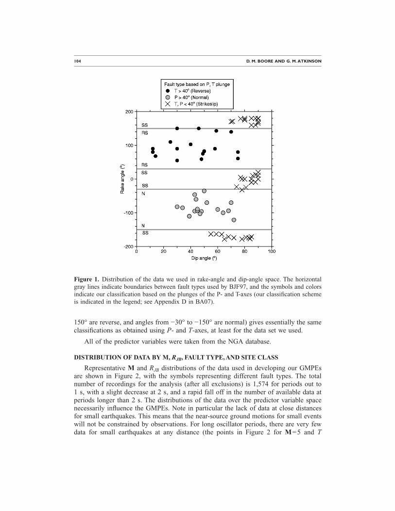
We also considered the effect of fault type (i.e., normal, strike-slip, and reverse). Thefault type was specified by the plunge of the P- and T-axes, as shown in the legend toFigure 1 (Appendix D of BA07 contains a more complete description). While there aresome advantages to using P- and T-axes, Figure 1 shows that the simple classificationused by BJF97 (rakes angles within 30° of horizontal are strike-slip, angles from 30° to

Table 1. (cont.)

NAME YEAR MODY M DIPDEPTH

(km) TYPE NOBSRJB

RANGE EQID

Northwest China-01 1997 0405 5.90 68 23 S 2 12–49 153Northwest China-02 1997 0406 5.93 30 31 N 2 20–37 154Northwest China-04 1997 0415 5.80 43 22 N 2 21–35 156Kocaeli, Turkey 1999 0817 7.51 88 15 S 26 1–316 136Chi-Chi, Taiwan 1999 0920 7.62 30 7 R 380 0–169 137Hector Mine 1999 1016 7.13 77 5 S 82 10–233 158Düzce, Turkey 1999 1112 7.14 65 10 S 22 0–188 138Yountville 2000 0903 5.00 90 10 S 24 8–94 160Big Bear-02 2001 0210 4.53 90 9 S 41 22–92 161Mohawk Val, Portola 2001 0810 5.17 81 4 S 6 67–126 162Anza-02 2001 1031 4.92 78 15 S 72 10–133 163Gulf of California 2001 1208 5.70 59 10 S 11 72–130 164CA/Baja Border Area 2002 0222 5.31 74 7 S 9 40–97 165Gilroy 2002 0514 4.90 84 10 S 34 2–130 166Yorba Linda 2002 0903 4.27 88 7 S 12 6–36 167Nenana Mountain,Alaska

2002 1023 6.70 90 4 S 33 105–280 168

Denali, Alaska 2002 1103 7.90 71 5 S 23 0–276 169Big Bear City 2003 0222 4.92 72 6 S 33 24–146 170


150° are reverse, and angles from −30° to −150° are normal) gives essentially the sameclassifications as obtained using P- and T-axes, at least for the data set we used.

All of the predictor variables were taken from the NGA database.

DISTRIBUTION OF DATA BY M, RJB, FAULT TYPE, AND SITE CLASS

Representative M and RJB distributions of the data used in developing our GMPEsare shown in Figure 2, with the symbols representing different fault types. The totalnumber of recordings for the analysis (after all exclusions) is 1,574 for periods out to1 s, with a slight decrease at 2 s, and a rapid fall off in the number of available data atperiods longer than 2 s. The distributions of the data over the predictor variable spacenecessarily influence the GMPEs. Note in particular the lack of data at close distancesfor small earthquakes. This means that the near-source ground motions for small eventswill not be constrained by observations. For long oscillator periods, there are very fewdata for small earthquakes at any distance (the points in Figure 2 for M=5 and T

Figure 1. Distribution of the data we used in rake-angle and dip-angle space. The horizontalgray lines indicate boundaries between fault types used by BJF97, and the symbols and colorsindicate our classification based on the plunges of the P- and T-axes (our classification schemeis indicated in the legend; see Appendix D in BA07).


=10 s are all from a single event—the 2000 Yountville, California earthquake), so themagnitude scaling at long periods will be poorly determined for small magnitudes.

The widest range of magnitudes is for strike-slip earthquakes (4.3–7.9), while thenarrowest range is for normal-slip earthquakes (5.3–6.9). This suggests that the magni-tude scaling is better determined for strike-slip than for normal-slip earthquakes—aproblem that we circumvented by using a common magnitude scaling for all types ofevents, as discussed later.

The bulk of the data are from class C and D sites, which range from soft rock to firmsoil; very few data were from class A sites (hard rock). More detail can be found inAppendix A, which includes two possible sets of VS30 values to use in evaluating ourequations for a particular NEHRP site class.

THE EQUATIONS

Following the philosophy of Boore et al. (1993, 1994, 1997), we seek simple func-tional forms for our GMPEs, with the minimum required number of predictor variables.We started with the simplest reasonable form for the equations (that used in BJF97), andthen added complexity as demanded by comparisons of the predictions of ground mo-tions from the simplest equations with the observed ground motions. The selection offunctional form was heavily guided by subjective inspection of nonparametric plots ofdata; many such plots were produced and studied before commencing the regressionanalysis. For example, the BJF97 equations modeled the far-source attenuation of am-

Figure 2. Distribution of data used to derive our regression equations for PGA and for PSA ata period 10.0 s, differentiated by fault type (points with RJB less than 0.1 km plotted at 0.1 km).The overall distributions for periods less than about 4 s are similar to those for PGA, althoughthere are fewer recordings (the number of available recordings decreases noticeably for periodslonger than 2 s).


plitudes with distance by a simple function that had no magnitude dependence and nocurvature at greater distances. This form appeared sufficient for the maximum distancerange of 80 km specified for the BJF97 GMPEs. The data, however, clearly show thatcurvature of the line is required to accommodate the effects of anelastic attenuationwhen modeling data beyond 80 km; furthermore, the data show that the effective geo-metric spreading factor is dependent on magnitude. To accommodate these trends, we(1) added an “anelastic” coefficient to the form of the equations, in which ln Y is pro-portional to R (where Y is the response variable), and (2) introduced a magnitude-dependent “geometrical spreading” term, in which ln Y is proportional to ln R and theproportionality factor is a function of M. These features allow the equations to predictamplitudes to 400 km; the larger size of the NGA database at greater distances and forlarger magnitudes, in comparison to that available to BJF97, enabled robust determina-tion of the additional coefficients. Our functional form does not include such factors asdepth-to-top of rupture, hanging wall/footwall terms, or basin depth, because residualanalysis does not clearly show that the introduction of such factors would improve theirpredictive capabilities on average. The equations are data-driven and make little use ofsimulations. They include only those terms that are truly required to adequately fit theobservational database, according to our analysis. Our equations may provide a usefulalternative to the more complicated equations provided by other NGA models, as theywill be easier to implement in many applications.

Our equation for predicting ground motions is:

ln Y = FM�M� + FD�RJB,M� + FS�VS30,RJB,M� + ��T, �1�

In this equation, FM, FD, and FS represent the magnitude scaling, distance function, andsite amplification, respectively. M is moment magnitude, RJB is the Joyner-Boore dis-tance (defined as the closest distance to the surface projection of the fault, which is ap-proximately equal to the epicentral distance for events of M�6), and the velocity VS30

is the inverse of the average shear-wave slowness from the surface to a depth of 30 m.The predictive variables are M, RJB, and VS30; the fault type is an optional predictivevariable that enters into the magnitude scaling term as shown in Equation 5a and 5b be-low. � is the fractional number of standard deviations of a single predicted value of ln Yaway from the mean value of ln Y (e.g., �=−1.5 would be 1.5 standard deviationssmaller than the mean value). All terms, including the coefficient �T, are period depen-dent. �T is computed using the equation

�T = ��2 + �2, �2�

where � is the intra-event aleatory uncertainty and � is the inter-event aleatory uncer-tainty (this uncertainty is slightly different for cases where fault type is specified andwhere it is not specified; we distinguish these cases by including a subscript on �).


THE DISTANCE AND MAGNITUDE FUNCTIONS

The distance function is given by:

FD�RJB,M� = �c1 + c2�M − Mref��ln�R/Rref� + c3�R − Rref� , �3�

where

R = �RJB2 + h2 �4�

and c1, c2, c3, Mref, Rref, and h are the coefficients to be determined in the analysis.

The magnitude scaling is given by:

a) M�Mh

FM�M� = e1U + e2SS + e3NS + e4RS + e5�M − Mh� + e6�M − Mh�2, �5a�b) M�Mh

FM�M� = e1U + e2SS + e3NS + e4RS + e7�M − Mh� , �5b�

where U, SS, NS, and RS are dummy variables used to denote unspecified, strike-slip,normal-slip, and reverse-slip fault type, respectively, as given by the values in Table 2,and Mh, the “hinge magnitude” for the shape of the magnitude scaling, is a coefficient tobe set during the analysis.

SITE AMPLIFICATION FUNCTION

The site amplification equation is given by:

FS = FLIN + FNL, �6�

where FLIN and FNL are the linear and nonlinear terms, respectively.

The linear term is given by:

FLIN = blin ln�VS30/Vref� , �7�

where blin is a period-dependent coefficient, and Vref is the specified reference velocity�=760 m/s�, corresponding to NEHRP B/C boundary site conditions; these coefficients

Table 2. Values of dummy variables for differentfault types

Fault Type U SS NS RS

Unspecified 1 0 0 0Strike-slip 0 1 0 0Normal 0 0 1 0Thrust/reverse 0 0 0 1


were prescribed based on the work of Choi and Stewart (2005; hereafter “CS05”); theyare empirically based but were not determined by the regression analysis in our study.

The nonlinear term is given by:

a) pga4nl�a1:

FNL = bnl ln�pga � low/0.1� �8a�b) a1�pga4nl�a2:

FNL = bnl ln�pga � low/0.1� + c�ln�pga4nl/a1��2 + d�ln�pga4nl/a1��3 �8b�c) a2�pga4nl:

FNL = bnl ln�pga4nl/0.1� �8c�

where a1 �=0.03 g� and a2 �=0.09 g� are assigned threshold levels for linear and non-linear amplification, respectively, pga � low �=0.06 g� is a variable assigned to transitionbetween linear and nonlinear behaviors, and pga4nl is the predicted PGA in g for Vref

=760 m/s, as given by Equation 1 with FS=0 and �=0. The three equations for the non-linear portion of the soil response (Equation 8a–8c) are required for two reasons: 1) toprevent the nonlinear amplification from increasing indefinitely as pga4nl decreases and2) to smooth the transition from linear to non-linear behavior. The coefficients c and d inEquation 8b are given by

c = �3�y − bnl�x�/�x2 �9�

and

d = − �2�y − bnl�x�/�x3, �10�

where

�x = ln�a2/a1� �11�

and

�y = bnl ln�a2/pga � low� . �12�The nonlinear slope bnl is a function of both period and VS30 as given by:

a) VS30�V1:

bnl = b1. �13a�b) V1�VS30�V2:

bnl = �b1 − b2�ln�VS30/V2�/ln�V1/V2� + b2. �13b�c) V2�VS30�Vref:

bnl = b2 ln�VS30/Vref�/ln�V2/Vref� . �13c�


d) Vref�VS30:

bnl = 0.0. �13d�

where V1=180 m/s, V2=300 m/s, and b1 and b2 are period-dependent coefficients (andconsequently, bnl is a function of period as well as VS30). These equations are a simplifiedversion of those used by CS05.

DETERMINATION OF COEFFICIENTS

METHODOLOGY

The selected response variables in the NGA database were first corrected to obtainthe equivalent observations for the reference velocity of 760 m/s, using Equations 6, 7,8a–8c, 9–12, and 13a–13d and an equation for pga4nl developed early in the project,using only data for which RJB�80 km and VS30�360 m/s (see BA07 for details). Wethen regressed the site-corrected observations to Equation 1 to determine FD and FM.Because the observations had all been corrected to the reference condition, we set FS

=0, simplifying the regression. The analyses were performed using the two-stage regres-sion discussed by Joyner and Boore (1993, 1994); the first stage determines the distancedependence (as well as event terms used in the second stage and the intra-event aleatoryvariability, �), and the second stage determines the magnitude dependence (and theinter-event variability, �). All regressions were done period-by-period; there was nosmoothing of the coefficients that were determined by the regression analyses (althoughsome of the constrained coefficients were smoothed). (Our “event term” is the average ofthe ln Y values for a given event, adjusted to the reference velocity and a reference dis-tance (760 m/s and 1 km, respectively, in our study). This differs from the “event term”that is derived in a random effects model. This latter term is more precisely called a“random effect for a given event” (e.g., Abrahamson and Youngs 1992). The residualsfrom our Stage 2 regression are equivalent to this alternate meaning of “event term.”)

Site Amplification

Because corrections for site amplification were made before doing the first-stage andsecond-stage regressions, we discuss the determination of the site amplification coeffi-cients first. The coefficients in the site-response equations were based on the work ofCS05, rather than determined by our regression analysis. The coefficients needed toevaluate the site-response equations are listed in Tables 3 and 4. Note that for the refer-ence velocity of 760 m/s, FLIN=FNL=FS=0. Thus the soil amplifications are specifiedrelative to motions that would be recorded on a B/C boundary site condition.

The rationale for pre-specifying the site amplifications is that the NGA database maybe insufficient to determine simultaneously all coefficients for the nonlinear soil equa-tions and the magnitude-distance scaling, due to trade-offs that occur between param-eters, particularly when soil nonlinearity is introduced. It was therefore deemed prefer-able to “hard-wire” the soil response based on the best-available empirical analysis in


the literature, and allow the regression to determine the remaining magnitude and dis-tance scaling factors. It is recognized that there are implicit trade-offs involved, and thata change in the prescribed soil response equations would lead to a change in the derivedmagnitude and distance scaling. Note, however, that our prescribed soil response terms

Table 3. Period-dependent site-amplificationcoefficients

Period blin b1 b2

PGV −0.600 −0.500 −0.06PGA −0.360 −0.640 −0.140.010 −0.360 −0.640 −0.140.020 −0.340 −0.630 −0.120.030 −0.330 −0.620 −0.110.050 −0.290 −0.640 −0.110.075 −0.230 −0.640 −0.110.100 −0.250 −0.600 −0.130.150 −0.280 −0.530 −0.180.200 −0.310 −0.520 −0.190.250 −0.390 −0.520 −0.160.300 −0.440 −0.520 −0.140.400 −0.500 −0.510 −0.100.500 −0.600 −0.500 −0.060.750 −0.690 −0.470 0.001.000 −0.700 −0.440 0.001.500 −0.720 −0.400 0.002.000 −0.730 −0.380 0.003.000 −0.740 −0.340 0.004.000 −0.750 −0.310 0.005.000 −0.750 −0.291 0.007.500 −0.692 −0.247 0.00

10.000 −0.650 −0.215 0.00

Table 4. Period-independent site-amplificationcoefficients

Coefficient Value

a1 0.03 gpga � low 0.06 ga2 0.09 gV1 180 m/sV2 300 m/sVref 760 m/s


are similar to those adopted by other NGA developers who used different approaches;thus there appears to be consensus as to the appropriate level for the soil responsefactors.

The details of setting the coefficients for the soil response equations are as follows.The linear amplification coefficients blin were adopted from CS05. As shown in Figure 3,they are similar to the linear soil coefficients derived by BJF97. CS05 do not providecoefficients for periods beyond 5 s. To determine coefficients for longer periods, we ex-trapolated the blin values as shown on Figure 3. As periods get very long ��5 s�, wewould expect the relative linear site amplification to decrease (and a trend in this direc-tion has been found by some of the other NGA developers). For this reason, we subjec-tively decided on the linear trend in terms of log period shown in Figure 3 as the basisfor choosing the values for the longer periods.

The nonlinear slope factor bnl depends on VS30 through the equations given above.Our equations define a somewhat simpler relation than that used by CS05. We comparethe two definitions of the coefficient bnl for periods of 0.2 and 3.0 s in Figure 4. Thevalues of bnl at the hinge points VS30=V1 and VS30=V2 are given by the coefficients b1

and b2, respectively, and these are functions of period. We use CS05’s values for mostperiods. To extend the value of b1 to periods longer than 5 s we fit two quadratic curvesto the CS05 values: one for all of the values and another for values corresponding toperiods greater than 0.2 s; the results were similar (see BA07 for a graph). We based ourvalue of b1 at periods of 7.5 s and 10 s on the quadratic fit to all of the CS05 values.

Figure 3. Coefficient controlling linear amplification, as function of period. Values used inequations in this report indicated by the black dots.


This curve was also used for the value at 5 s, but the results of using the CS05 value at5 s versus our value makes almost no difference in the predicted ground motions for 5 speriods.

We point out a potential confusion in terminology: according to Equation 8c, FNL

=0.0 when pga4nl=0.1 g. Does this mean that there is no nonlinear amplification forthis level of rock motion? Not necessarily. The amplification for this value of pga4nl isgiven entirely by the FLIN term because the motions used by CS05 to derive the “linear”amplifications �FLIN� had an approximate mean log PGA for most site categories close to0.1 g. FNL is not necessarily zero, however, for values of pga4nl less than and greaterthan 0.1 g. So although the amplification at pga4nl=0.1 g is completely determined byFLIN, the amplification could implicitly include the nonlinear component that applies forvalues of pga4nl near 0.1 g. CS05 use only Equation 8c to describe the nonlinear am-plification, and they do not limit the nonlinear response to pga4nl�0.1 g. It is clearfrom Figure 3 of CS05 and the comment on p. 24 of their paper that they consider Equa-tion 8c to be valid for pga4nl from 0.02 to 0.8 g. This means that the total amplification�FS� can be greater than the “linear” amplification �FLIN� for small values of pga4nl;their nonlinear amplification continues to increase without bound as pga4nl decreases.We made an important modification to the CS05 procedure to prevent nonlinear ampli-fication from extending to small values of pga4nl, by capping the amplifications at a lowvalue of pga4nl �0.03 g�. Simply terminating the nonlinear amplification at a fixed valueof pga4nl results in a kink in plots of ground motion vs. distance. For that reason weincluded a transition curve, as given in Equation 8b.

The total amplification for a short �0.2 s� and a long �3.0 s� period oscillator isshown in Figure 5 as a function of pga4nl for a range of VS30. At short periods the non-linear term can result in a significant reduction of motions on sites underlain by rela-tively low velocities. At long periods soil nonlinearity is still important, but the net soilresponse effect is an amplification, even for large values of pga4nl. For periods longerthan 0.75 s (see Table 3) there is no nonlinear contribution to the amplification forVS30�300 m/s

It should be noted that the empirical studies on which the soil amplification functions

Figure 4. Comparison of slope that controls nonlinear amplification function.


were based contained very few data for hard sites, with VS30�1,000 m/s. The amplifi-cation functions are probably reasonable for values of VS30 up to about 1,300 m/s, butshould not be applied for very hard rock sites �VS30�1500 m/s�.

Distance Dependence (Stage 1)

The distance dependence of ground motion is determined in the first-stage regres-sion, where the dependent response variable is PGA, PGV, or PSA at a selected period,in each case corrected to the reference velocity of 760 m/s by subtracting FS as definedin Equations 6, 7, 8a–8c, 9–12, and 13a–13d from ln Yobserved. The corrected responsevariables for our selected subset of the NGA data set (using the exclusion criteria dis-cussed earlier), with distances out to 400 km, are regressed against distance using Equa-tion 14, which is the same as Equation 2 but with dummy variables �c0�event�� added torepresent the event term for each earthquake.

FD�RJB,M� = c0�event� + �c1 + c2�M − Mref��ln�R/Rref� + c3�R − Rref� �14�

In this equation, “c0�event�” is shorthand for the sum

�c0�11 + �c0�22 + ¯ + �c0�NENE, �15�

where �c0�j is the event term for event j, j equals 1 for event j and zero otherwise, andNE is the number of earthquakes.

There are several significant issues in performing this regression. One is that re-gional differences in attenuation are known to exist (e.g., Boore 1989, Benz et al. 1997),

Figure 5. Combined amplification for T=0.2 s and T=3.0 s as function of pga4nl, for suite ofVS30. Note at short periods (left graph), purely linear amplification does not occur on soft soilsuntil pga4nl�0.03 g.


even within relatively small regions such as California (e.g., Bakun and Joyner 1984,Boatwright et al. 2003, Hutton and Boore 1987, Mori and Helmberger 1996). We ignorethis potential pitfall and assume that the distance part of the GMPEs apply for crustalearthquakes in all active tectonic regimes represented by the NGA database. This is areasonable initial approach, as the significance of regional effects can be tested later byexamining residual trends (model errors) for subsets of data organized by region. Thesecond difficulty is more problematic: the data in the NGA Flatfile become increasinglysparse for distances beyond about 80 to 100 km, especially for moderate events. Thismakes it difficult, if not impossible, to obtain a robust simultaneous determination of c1

and c3 (slope and curvature). To overcome this database limitation, we have used addi-tional ground-motion data from California that are not in the NGA Flatfile, to first definethe “anelastic” term, c3, as a function of period. We then used these fixed values of c3 inthe regression of the NGA data set in order to determine the remaining coefficients.

Determination of c3 (anelastic term): The data used to determine c3 includes the datacompiled in the NGA database for three small California events, plus many more datafor these same events recorded by accelerometers at “broadband” stations in California;these additional data, compiled by J. Boatwright and L. Seekins, were not available fromthe traditional strong-motion data agencies used in compiling the NGA Flatfile. We alsoused response variables that we computed from 74 two-component recordings of the2004 Parkfield mainshock (M 6.0) in the determination of c3; these data were recordedafter the compilation of the NGA database had concluded. The numbers of stations pro-viding data for our analysis and the corresponding numbers of stations in the NGA Flat-file are given in Table 5 (see also Appendices M and N in BA07).

For the additional data for the three small California earthquakes, we used siteclasses assigned by Boatwright and Seekins to correct the response spectra to VS30

=760 m/s. For the Parkfield recordings we did not correct to a common value of VS30,as we were interested only in determining the distance function, and also because mea-sured values of VS30 were available at only a few sites. For all of the data from the fourevents we used spectra from the two horizontal components as if they were separate re-cordings (we did not combine the horizontal components). We did the regressions onthis data subset with c1 fixed at −0.5, −0.8, and −1.0. We set c2 to zero and solved for c3

and h. In other words, we fixed a single straight-line slope �c1�, and then determined thecurvature, c3, required to match the more rapid decay of the data at greater distances (c3

must be less than 0). We also solved for the near-source effective depth coefficient, h,

Table 5. Comparisons of numbers of stations in NGA Flatfile and in extended data set used todetermine anelastic coefficient

Earthquake # of Stations in NGA # of Stations Used by BA

2001 Anza �M 4.92� 73 1972002 Yorba Linda �M 4.27� 12 2072003 Big Bear City �M 4.92� 37 2622004 Parkfield �M 6.0� 0 74


required to match the less rapid increase of the data as distance decreases at close dis-tances. An event term that gives the relative amplitude level, �c0�, is determined for eachof the four earthquakes (these are the coefficients of the dummy variables for eachevent). Figure 6 compares the regression fits to the observations, where the observationshave been normalized to a common amplitude level by subtracting the event terms �c0�.We chose the c3 values determined for the case c1=−0.8 as the fixed c3 values to applyin the regression of the NGA data set because c1=−0.8 is a typical value determined inempirical regressions for the effective geometric slope parameter at intermediate periods(BJF97; this study).

As a broader check on the results from our four-event attenuation data set, we de-termined the best values of c3 and h to fit the distance functions determined in southernCalifornia from a much larger database, by Raoof et al. (1999). The equivalent values ofc3 and h implied by the Raoof et al. (1999) attenuation results are similar to those thatwe determined from our four-event analysis.

To assign values of c3 over the full period range required in the NGA project, we fita quadratic to the c3 values from the analysis of our four-event data subset. We did notallow the value of c3 at short periods to be less than that for PGA, thus placing an upperlimit on �c3� at �c3�=0.01151. Similarly, we fixed the values for long periods to be thatdetermined for T=3 s, thus placing a lower limit on �c3� of �c3�=0.00191 (we did notthink it physically plausible for the anelastic attenuation to increase with period at T�3 s).

We also constrained the c3 values for the PGV regressions to be that for the T=1.0 s regression. This choice is a compromise between the similarity in larger-

Figure 6. Normalized ground motions for four events, using extended data set (more data thanin NGA Flatfile). Black curve is regression fit obtained with constraints c1=−0.8 and c2=0.0.


magnitude scaling that we observed between PGV and PSA at 2 s and the recommen-dation of Bommer and Alarcón (2006) that PGV is related to PSA at 0.5 s.

Determination of h: It is desirable to constrain the pseudo-depth h in the regressionin order to avoid overlap in the curves for large earthquakes at very close distances. Wedid this by performing initial regressions with h as a free parameter, then modifying theresultant values of h as required to avoid overlap in the spectra at close distances (for thereference site condition of 760 m/s). In this regression, c1 was a free variable and c3was constrained to a set of initially-determined values. We fit the values determined withh as a free parameter with a quadratic, but we observed that the h value at 0.05 s fromthe quadratic fit was very small, much below that determined for PGA. We increased theh value at 0.05 s to match the value for a regression of PGA with h unconstrained, andrefit the quadratic with this change in the data points. We used the modified quadratic asthe basis for assigning h for all periods. The value of h at short periods was guided bythe unequivocal statement that PSA is equal to PGA at periods much less than 0.1 s. ForPGA, we adopted the value implied by the modified quadratic for the T=0.05 s oscilla-tor. We then assigned values of h for periods between 0.01 s and 0.05 s to be the sameas that for 0.05 s. Consistent with the convention adopted for the c3 coefficient, we usedthe value of h at 1 s for PGV.

These analyses established smooth, constrained values for c3 and h that facilitatedrobust and well behaved determinations of the remaining parameters by regression of theNGA database.

Determination of c1, c2, and �: With h and c3 constrained, we regressed the re-sponse variables of the NGA database to solve for c1 and c2 (Equation 3), along with theevent terms �c0� for each earthquake, using all data (subject to the exclusions discussedearlier) for distances less than 400 km. The c1 coefficient is the effective geometricspreading rate (slope) for an event of M=Mref, while the c2 coefficient provides a meansto describe magnitude-dependent distance decay (it changes the slope for events that aregreater or smaller than Mref). The intra-event aleatory uncertainty � is given by the stan-dard deviation of the residuals from the Stage 1 regression.

The regression used assigned values for the reference distance, Rref, at which near-source predictions are pegged, and for the reference magnitude, Mref, to which the mag-nitude dependence of the geometric spreading is referenced. The assigned values forthese reference values are arbitrary and are largely a matter of convenience. For Mref, wechose a value of 4.5, since this is the approximate magnitude of much of the data usedto determine the fixed c3 coefficients; this choice means that the magnitude dependenceof the slope will be referenced to that observed for small events. For Rref, we use thevalue of 1 km. This is convenient because the curves describing the distance dependencepivot around R=Rref. The curves for larger magnitudes are flatter than for smaller mag-nitudes, which can lead to those curves being below the curves for smaller magnitudes atdistances less than the pivot distance. This was avoided by choosing Rref=1 km, al-though any value such that Rref�min�h�, where the minimum is taken over all periods,


would prevent undesirable overlapping of prediction curves near the source (i.e. we wantto ensure that R will always be greater than the pivot distance of Rref, even when RJB

=0 km).

Magnitude Dependence (Stage 2)

The event terms (coefficients �c0�j in Equation 14 from the Stage 1 regression wereused in a weighted Stage 2 regression to determine the magnitude scaling of the re-sponse variables. As discussed in Joyner and Boore (1993), the Stage 2 weighted regres-sion was iterative in order to solve for the inter-event variability �. The basic form weselected for the magnitude scaling is a quadratic, similar to the form used by BJF97.However, we imposed a constraint that the quadratic not reach its maximum at M�8.5, in order to prevent “oversaturation” (the prediction of decreasing amplitudes withincreasing magnitude). The following algorithm was used to implement the constrainedquadratic magnitude dependence:

1. Fit the event terms �c0�j for a given period to a second-order polynomial. If theM for which the quadratic starts to decrease �Mmax� is greater than 8.5, weadopt this regression for the magnitude dependence for this period.

2. If Mmax for a given period is less than 8.5, we perform a two-segment regres-sion, hinged at Mh (described below), with a quadratic for M�Mh and a linearfunction for Mh�M. If the slope of the linear function is positive, we adopt thistwo-segment regression for the magnitude dependence for this period.

3. If the slope of the linear segment is negative, we redo the two-segment regres-sion for that period, constraining the slope of the line above Mh to be 0.0. Notethat the equations for almost all periods less than or equal to 1.0 s required theconstraint of zero slope; this is telling us that for short periods the data actuallyindicate oversaturation. We felt that because of limited data and knowledge,oversaturation was too extreme at this stage of equation development, and wechose to impose saturation rather than allow the data to dictate an oversaturatedform. More observations from ground motions near large earthquakes, as wellas theoretical simulations using dynamic rupture models (e.g., Schmedes andArchuleta, 2007) may give us confidence in allowing oversaturation in futureversions of GMPEs.

Choice of Mh: The parameter Mh is the hinge magnitude at which the constrainedmagnitude scaling in the two-segment regression changes from the quadratic form to thelinear form. Subjective inspection of nonparametric plots of data clearly indicated thatnear-source ground motions at short periods do not get significantly larger with increas-ing magnitude, beyond a magnitude in the range of 6.5 to 7, and therefore we set Mh

within this range.

Fault-Type Dependence: Plots of event terms against magnitude (presented later)showed that normal-fault earthquakes have amplitudes that are consistently below thosefor strike-slip and reverse earthquakes for most periods (others have found similar re-sults, including Spudich et al. 1999, Bommer et al. 2003, and Ambraseys et al. 2005).We used this observation to guide our determination of the dependence on fault type. Wefirst grouped the data from all fault types together and solved for the coefficients e , e ,
1 5


e6, e7, and e8 in Equation 5a and 5b), setting e2, e3, and e4 to 0.0. The regression wasthen repeated, fixing the coefficients e5, e6, e7, and e8 to the values obtained when lump-ing all fault types together, and solving for the coefficients e2, e3, and e4 of the fault typedummy variables SS, NS, and RS. Thus we have constrained the relative scaling of am-plitudes with magnitude to be the same for all event types, but we allow an offset in theaverage predicted amplitude level according to the fault mechanism. The inter-eventaleatory uncertainty �� was slightly different for these two cases, so subscripts “U” and“M” were used to distinguish between unspecified and specified fault type, respectively,in the table of aleatory uncertainties. Note that the term “unspecified” is strictly appli-cable to a random selection of an earthquake from the distribution of fault types used inour analysis; it is an accurate description of a truly random selection from all earth-quakes only to the extent that the distribution of all fault types is equal to the distributionused in our analysis.

All analyses were done using Fortran programs developed by the first author, in somecases incorporating legacy code from programs and subroutines written by W. B. Joyner.

RESULTS

COEFFICIENTS OF THE EQUATIONS

The coefficients for the GMPEs are given in Tables 3, 4, and 6–8. The coefficientsare for ln Y, where Y has units of g for PSA and PGA and cm/s for PGV. The units ofdistance and velocity are km and m/s, respectively. The equation for pga4nl is the sameas for PGA, with VS30�760 m/s (for which FS=0) (Boore and Atkinson, 2008).

There are no normal-fault data are in our data set for an oscillator period of 10 s, andthus formally we could not obtain the coefficient e3 for that period; the value in Table 7was obtained using the assumption that the ratio of motions for normal and unspecifiedfaults is the same for periods of 7.5 s and 10 s. With this assumption, e3�10s�=e1�10s�+ �e3�7.5s�−e1�7.5s��.

Fit of the Stage 1 Regressions

BA07 contains a series of graphs showing the observations in comparison to theStage 1 regression predictions. These figures provide a visual test of the ability of ourfunctional form to represent the distance dependence of the response variables. A moreprecise way of looking for systematic mismatches between predictions and observationsis to plot the residuals from the Stage 1 analysis, defined as the ratio of observed topredicted ground motions. Figure 7 shows residuals as a function of distance for PGAand for PSA at 10 s; these span the range of seismic intensity measures included in ourequations (the graphs of residuals for PSA at most oscillator periods are similar to thatfor PGA in Figure 7—see BA07 for a complete set of graphs). For the sake of clarity, wehave separated the residuals into different magnitude ranges and for two specific earth-quakes in Figure 7. Log residuals averaged over distance bins 0.1 log unit in width andmagnitude bins 1 unit in width are shown in Figure 8 for two representative periods; thegraphs are grouped by values of VS30. While there are some small departures from a nullresidual (values of 1 and 0 in Figures 7 and 8, respectively), there are no significant


trends in magnitude, distance, or shear-wave velocity. We therefore judge the fit betweenobservations and our predictions to be reasonable. In particular, we note that the im-posed soil response coefficients appear to be adequate, as evidenced by the apparent fitover the three distinct ranges of shear-wave velocity used in Figure 8; the fit is good atboth short and large distances over all magnitude ranges, which implicitly supports thedegree of nonlinearity that was specified.

Fit of the Stage 2 Regressions

Figure 9 is a plot of the antilog of the event terms �c0�j from the Stage 1 regressionas a function of magnitude, with the Stage 2 regression fit to these terms superimposed.The fault type for each earthquake is indicated, as are curves for fault type unspecifiedand for strike-slip, normal, and thrust/reverse faults (the fault type is indicated by thecolor of the symbols). The functional form provides a reasonable fit to the near-source

Table 6. Distance-scaling coefficients (Mref=4.5 andRref=1.0 km for all periods, except Rref=5.0 km forpga4nl)

Period c1 c2 c3 h

PGV −0.87370 0.10060 −0.00334 2.54PGA −0.66050 0.11970 −0.01151 1.350.010 −0.66220 0.12000 −0.01151 1.350.020 −0.66600 0.12280 −0.01151 1.350.030 −0.69010 0.12830 −0.01151 1.350.050 −0.71700 0.13170 −0.01151 1.350.075 −0.72050 0.12370 −0.01151 1.550.100 −0.70810 0.11170 −0.01151 1.680.150 −0.69610 0.09884 −0.01113 1.860.200 −0.58300 0.04273 −0.00952 1.980.250 −0.57260 0.02977 −0.00837 2.070.300 −0.55430 0.01955 −0.00750 2.140.400 −0.64430 0.04394 −0.00626 2.240.500 −0.69140 0.06080 −0.00540 2.320.750 −0.74080 0.07518 −0.00409 2.461.000 −0.81830 0.10270 −0.00334 2.541.500 −0.83030 0.09793 −0.00255 2.662.000 −0.82850 0.09432 −0.00217 2.733.000 −0.78440 0.07282 −0.00191 2.834.000 −0.68540 0.03758 −0.00191 2.895.000 −0.50960 −0.02391 −0.00191 2.937.500 −0.37240 −0.06568 −0.00191 3.00

10.000 −0.09824 −0.13800 −0.00191 3.04


amplitude data. Note that the magnitude scaling for T=10 s at M�6.5 is strongly con-trolled by the data from only one small earthquake (2000 Yountville, M 5.0), and maytherefore be unreliable for M�6.5.

Predictions of PSA from Combined Stage 1 and Stage 2 Regressions

Graphs of PSA predicted from our equations for three values of RJB and four mag-nitudes are shown in Figure 10. The curves for the larger earthquakes tend to squeezetogether for periods near 0.2–0.3 s, probably a reflection of the pinching together of theeffective geometric spreading factor for these periods. But otherwise the PSA are quitesmooth, especially considering that many of the coefficients were determined indepen-dently for each period.

Plots of PSA as a function of distance are shown in Figure 11 for two representativeperiods (see BA07 for plots at other periods). The figure is for VS30=760 m/s (NEHRPB/C boundary).

The effect of VS30 on predicted ground-motion amplitude is shown in Figure 12.Nonlinear soil amplification causes the curves to cross, such that at close distances lower

Table 7. Magnitude-scaling coefficients

Period e1 e2 e3 e4 e5 e6 e7 Mh

PGV 5.00121 5.04727 4.63188 5.08210 0.18322 −0.12736 0.00000 8.50PGA −0.53804 −0.50350 −0.75472 −0.50970 0.28805 −0.10164 0.00000 6.750.010 −0.52883 −0.49429 −0.74551 −0.49966 0.28897 −0.10019 0.00000 6.750.020 −0.52192 −0.48508 −0.73906 −0.48895 0.25144 −0.11006 0.00000 6.750.030 −0.45285 −0.41831 −0.66722 −0.42229 0.17976 −0.12858 0.00000 6.750.050 −0.28476 −0.25022 −0.48462 −0.26092 0.06369 −0.15752 0.00000 6.750.075 0.00767 0.04912 −0.20578 0.02706 0.01170 −0.17051 0.00000 6.750.100 0.20109 0.23102 0.03058 0.22193 0.04697 −0.15948 0.00000 6.750.150 0.46128 0.48661 0.30185 0.49328 0.17990 −0.14539 0.00000 6.750.200 0.57180 0.59253 0.40860 0.61472 0.52729 −0.12964 0.00102 6.750.250 0.51884 0.53496 0.33880 0.57747 0.60880 −0.13843 0.08607 6.750.300 0.43825 0.44516 0.25356 0.51990 0.64472 −0.15694 0.10601 6.750.400 0.39220 0.40602 0.21398 0.46080 0.78610 −0.07843 0.02262 6.750.500 0.18957 0.19878 0.00967 0.26337 0.76837 −0.09054 0.00000 6.750.750 −0.21338 −0.19496 −0.49176 −0.10813 0.75179 −0.14053 0.10302 6.751.000 −0.46896 −0.43443 −0.78465 −0.39330 0.67880 −0.18257 0.05393 6.751.500 −0.86271 −0.79593 −1.20902 −0.88085 0.70689 −0.25950 0.19082 6.752.000 −1.22652 −1.15514 −1.57697 −1.27669 0.77989 −0.29657 0.29888 6.753.000 −1.82979 −1.74690 −2.22584 −1.91814 0.77966 −0.45384 0.67466 6.754.000 −2.24656 −2.15906 −2.58228 −2.38168 1.24961 −0.35874 0.79508 6.755.000 −1.28408 −1.21270 −1.50904 −1.41093 0.14271 −0.39006 0.00000 8.507.500 −1.43145 −1.31632 −1.81022 −1.59217 0.52407 −0.37578 0.00000 8.50

10.000 −2.15446 −2.16137 −2.53323 −2.14635 0.40387 −0.48492 0.00000 8.50


values of VS30 (softer sites) will have lower predicted amplitudes than stiffer sites, due tononlinear deamplification. The effect is more pronounced at short periods than at longperiods.

Surface Slip vs. No-Surface Slip Earthquakes

Several authors (e.g., Somerville and Pitarka 2006) have proposed that the high-frequency ground motions from earthquakes with faults that break to the surface aresmaller than from those with faults that remain buried. We search for evidence of thiseffect in Figure 13, which shows the event-term residuals from the Stage 1 regressionplotted against M for the two classes of earthquakes. The first thing to notice is that mostsurface-slip earthquakes correspond to larger magnitudes, with almost no buried rup-tures for magnitude greater than M=7. For this reason any reduction in motions forsurface-slip earthquakes will be mapped into reduced magnitude scaling in the Stage 2magnitude regression. In order to differentiate magnitude scaling from the effects of sur-face versus buried rupture, data from both class of rupture are needed for the same range

Table 8. Aleatory uncertainties (�: intra-event uncertainty; �: inter-eventuncertainty; �T: combined uncertainty ��2+�2�; subscripts U, M for faulttype unspecified and specified, respectively)

Period � �U �TU �M �TM

PGV 0.500 0.286 0.576 0.256 0.560PGA 0.502 0.265 0.566 0.260 0.5640.010 0.502 0.267 0.569 0.262 0.5660.020 0.502 0.267 0.569 0.262 0.5660.030 0.507 0.276 0.578 0.274 0.5760.050 0.516 0.286 0.589 0.286 0.5890.075 0.513 0.322 0.606 0.320 0.6060.100 0.520 0.313 0.608 0.318 0.6080.150 0.518 0.288 0.592 0.290 0.5940.200 0.523 0.283 0.596 0.288 0.5960.250 0.527 0.267 0.592 0.267 0.5920.300 0.546 0.272 0.608 0.269 0.6080.400 0.541 0.267 0.603 0.267 0.6030.500 0.555 0.265 0.615 0.265 0.6150.750 0.571 0.311 0.649 0.299 0.6451.000 0.573 0.318 0.654 0.302 0.6471.500 0.566 0.382 0.684 0.373 0.6792.000 0.580 0.398 0.702 0.389 0.7003.000 0.566 0.410 0.700 0.401 0.6954.000 0.583 0.394 0.702 0.385 0.6985.000 0.601 0.414 0.730 0.437 0.7447.500 0.626 0.465 0.781 0.477 0.787

10.000 0.645 0.355 0.735 0.477 0.801


Figure 7. Stage 1 residuals, separated by magnitude, for PGA and T=10 s PSA (these span therange of possibilities; see BA07 for more plots). The residuals for the 1999 Chi-Chi earthquakeare shown separately, in the bottom two graphs.


of magnitudes. As seen in Figure 13, it is only for strike-slip earthquakes that there ismore than one of each class of earthquake in a common magnitude range (there are sev-eral strike-slip events of 5.7–6.7 in both classes). There is no indication for these earth-quakes that the event-term residuals are systematically different for the two classes ofdata. Therefore, there was no need to include dummy variables for surface-slip/buriedearthquakes in our functional forms. As confidence in simulations from dynamic modelsof rupture propagation increases, or if additional data change our understanding, it mightbe that in the future we will add a buried/surface faulting term to the equations. By do-ing so, the apparent saturation of the magnitude scaling would not be as dramatic (i.e.,the larger earthquakes are entirely surface slip events, and if these produce smallerground motions than buried events, as has been suggested by Somerville and colleagues

Figure 8. Stage 1 regression residuals �log10 units� for 0.2-s and 3-s response spectra, aver-aged over distance bins 0.1 log unit in width and magnitude bins 1 unit in width. Only bins withat least three observations are plotted. The standard error of the mean is shown for the middlemagnitude bin (6 to 7) only. Two ranges of shear-wave velocity are shown: 180–360 m/s (top),360–760 m/s (bottom). No residuals are shown for VS30�760 m/s because of the small num-ber of observations in that velocity range.


Figure 9. Y�event� (the antilog of the average of the log of the motions for each event adjustedto the reference distance of 1 km and the reference velocity of 760 m/s; in the terminology of

Equations 14 and 15, Y�event�=exp�c0�event��) and Stage 2 regression fits. Note that the samevertical scale was used for all graphs in order to compare the magnitude scaling from period toperiod.


(e.g., Somerville and Pitarka 2006), then there will be an apparent tendency for satura-tion if the events are not separated into two classes according to whether they break tothe surface or not).

Dependence of Stage 1 Residuals on Basin Depth

Another ground-motion effect that we searched for in the residuals of the Stage 1regression was that of basin depth. Basin-depth effects on ground-motion amplitudeshave been reported in empirical studies (Field, 2000; Choi et al. 2005), and from simu-lations (Day et al. 2008). One of the reasons that we did not include a basin-depth termin our equations is indicated in Figure 14, which shows the distribution of VS30 and a

Figure 10. PSA from our equations, as function of period. The spectra are shown for threedistances and four magnitudes, for fault type unspecified and VS30=760 m/s.


Figure 11. PSA from our equations, as a function of distance. The spectra are shown for mag-nitudes 5, 6, 7, and 8, for fault type unspecified and VS30=760 m/s. Note that the same verticalscale was used for both graphs in order to compare the magnitude scaling for the two periods.

Figure 12. PSA from our equations, as a function of distance for magnitude 7, fault type un-specified, and three values of VS30. Note that the same vertical scale was used for both graphs
in order to compare the magnitude scaling for the two periods.


measure of basin depth. The plot shows all data in the NGA Flatfile for which both VS30have been measured and basin depth have been estimated. It is clear that the softer sitesare in basins, and hence basin depth and VS30 are strongly correlated (this was foundpreviously by Choi et al. 2005, Figure 7). Therefore any basin depth effect will tend to

Figure 13. Antilogarithms of Stage 2 residuals, plotted against magnitude and differentiated byevents of different fault types, for which faults did or did not break to surface.

Figure 14. VS30 plotted against one measures of basin depth: the depth to a shear-wave velocityof 1.5 km/s. All values in the NGA Flatfile with basin depths and measured (rather than esti-
mated) values of VS30 are shown.


have been captured by the empirically-determined site amplification. To try to separatethe amplification and the basin-depth effects in the data would require use of additionalinformation or assumptions. Since we are opting for the simplest equations required bythe data, no attempt was made to break down the site-response function into basin depthand the amplification terms.

We searched for any uncaptured basin depth effect by examining the residuals of theStage 1 regressions. We find that the residuals have no dependence on basin depth, ex-cept for a trend to positive residuals (underprediction) for long periods at distances be-yond 80 km (by about a factor of 1.6), for sites having depth-to-1.5 km/s�700 m. (Thetrend for greater distances is shown in a figure not included here.) These residuals couldalso be due to regional variations in the distance function, along with correlations be-tween distance and the basin depth. Figure 15 contains plots of the Stage 1 residualsagainst the depth-to-VS30=1.5 km/s; only residuals for RJB�80 km are shown, in ordernot to map mismatches in the more distant attenuation into the residuals. There is noobvious dependence of the residuals on basin depth. But assuming that the positive re-siduals at distances greater than 80 km are due solely to a basin depth effect, the trendsindicate that our equations may underpredict long-period motions at large distancesfrom sites in deep basins. For shallower basins and at shorter distances, we find no basindepth effect. This is not surprising in light of the observations made above regarding thecorrelation between basin parameters and VS30. (Note: similar results were obtainedwhen the depth to 2.5 km/s was used as the measure of basin depth.) Another reason for

Figure 15. Stage 1 residuals plotted against depth to VS=1.5 km/s, differentiated by VS30, forRJB�80 km.


little apparent basin effect has to do with the way in which basins affect incoming waves;Choi et al. (2005) found a basin effect for sources inside the basin in which the motionswere recorded, but little effect for sources outside the basin; they attribute the differenceto the manner in which incoming waves are converted and refracted upon entering thebasin. As many of our data come from earthquakes that occurred outside the basins inwhich they were recorded, a similar explanation might apply to our finding.

Comparison of GMPEs Developed With and Without the 1999Chi-Chi Earthquake

Because the Chi-Chi earthquake forms a significant fraction of the data set we usedin developing our equations, it is important to see how the equations would change if thedata from the Chi-Chi earthquake were eliminated from both the Stage 1 and the Stage2 regressions. We therefore repeated the complete analysis without the Chi-Chi data.Figure 16 compares selected ground-motion intensity measures given by the two sets ofequations. The figure also shows the percent of data used in the regression analysis fromthe Chi-Chi earthquake (the number of Chi-Chi recordings is the numerator of the ratio).It is clear that the fraction of the data set contributed by the Chi-Chi earthquake in-creases with period, reaching 64% of the data set for a period of 10 s. For this reason itis not surprising that the predictions of 10 s PSA are quite different for the equationsdeveloped with and without the Chi-Chi data (the ordinate scales of all graphs in Figure16 are the same, to facilitate comparisons of the relations between the two predictionsbetween periods); at intermediate to short periods, however, the differences are not dra-matic. Interestingly, the differences can occur even at small magnitudes (despite the factthat we include only the Chi-Chi mainshock, not its aftershocks). We think the explana-tion of this apparent paradox is that the Chi-Chi earthquake is very well recorded andthus dominates the Stage 1 regression, for which each recording of an earthquake hasequal weight in determining the distance terms in the equations. These distance termsthen affect the event terms, and this in turn controls the magnitude scaling. We concludethat although the Chi-Chi earthquake affects the GMPEs, it is only a major controllingfactor in the predictions of PSA at periods of greater than 5 s.

Comparison of BA07 and BJF97 GMPEs

It is interesting to compare our new predicted ground motions with those from theBoore et al. (1997) (BJF97) equations. Figure 17 (top row) compares the magnitude-distance distribution of the data used in each study. It is apparent that many more dataare used in the new equations; the NGA data fill gaps at close distances for all magni-tudes, add more data at small magnitudes at all distances, add data for large magnitudes,and fill out the distribution so that no longer is there a strong correlation between dis-tance and magnitude in the data set. For this reason, the new equations provide a morerobust prediction of ground-motion amplitudes over a wide range of magnitudes anddistances.

We compare predicted ground motions from the BJF97 equations and from our cur-rent equations in Figure 17 (bottom row), for VS30=420 m/s, which is near the weightedgeometric mean of the velocities for the sites used in the BJF97 regression analysis. We


use the same scale for the ordinates in both graphs. The new and old equations predictsimilar amplitudes for M and RJB ranges for which data were available for the BJF97equation development. Large differences occur in regions of the magnitude-distancespace for which data were not available in BJF97; the differences in the predicted valuesof seismic ground-motion intensity are largely attributable to the overly-simplifieddistance-independent magnitude scaling used in the BJF97 equations.

At all periods, the new equations predict significantly smaller motions than do theBJF97 equations for large magnitudes. This is probably the most important change in thenew equations compared to the old equations. The difference in the predicted motions isparticularly large for T=1 s and M=7.5 (a factor of 2.4 at RJB=1 km). Almost no datawere available in BJF97 for M�7.5 and RJB�10 km (see Figure 17), so discrepancies

Figure 16. Comparisons of PSA for four periods from equations developed with and without1999 Chi-Chi mainshock. Ratios are number of Chi-Chi recordings used to develop final equa-tions divided by total number of recordings.


are not surprising. The BJF97 data were for RJB centered about 30 km. The discrepancybetween the predictions from the BJF97 and the new equations is not nearly as strong forRJB near 30 km as it is for RJB�10 km. Observed differences at RJB�30 km are likelydue to including more data for large earthquakes in our current equations. The values ofthe BJF97 motions at close distances are strongly controlled by the assumption ofdistance-independent M scaling (and therefore the scaling at close distances is driven bythe RJB�30 km data). The current equations allow for M-dependent distance scaling.Another effect that can reduce motions predicted from our equations at close distancesfrom large earthquakes is nonlinear site response, which is not included in BJF97.

The total aleatory uncertainties, as well as the intra- and inter-event uncertainties, aresignificantly larger for the new equations than for the BJF97 equations (e.g., for a periodof 0.2 s the total aleatory uncertainty is 0.60 for our equations and 0.44 for BJF97; morecomparisons can be found in Table 4.6 of BA07). We are not sure of the reasons for the

Figure 17. Top two graphs: Comparison of magnitude-distance distribution of data used byBJF97 and by BA08; bottom two graphs: PGA and T=1.0 s PSA predictions from BJF97 andfrom BA08 GMPEs.


differences, but we suspect the differences are due to a combination of more data pro-viding a better sample of the true uncertainty, as well as an increase in the uncertaintiesproduced by mixing data from regions for which the attenuation of the motions might bedifferent (see Douglas 2007, for a study of regional differences in ground-motion pre-diction). The larger sigma values will offset to some extent the smaller ground motionsfor large magnitudes in the construction of seismic hazard maps. However, it is a pointfor further investigation how the aleatory uncertainties should be implemented in hazardanalyses for a particular site, given that part of the aleatory uncertainty arises from mix-ing data from numerous regions.

GUIDELINES FOR USAGE

LIMITS ON PREDICTOR VARIABLES

We wish to emphasize that our equations should be used only for predictor variablesin these ranges:

• M=5–8

• RJB�200 km

• VS30=180–1300 m/sThese limits are subjective estimates based on the distributions of the recordings used todevelop the equations.

PREDICTIONS FOR OTHER MEASURES OF SEISMIC INTENSITY

The NGA GMPEs are for the GMRotI measure of seismic intensity. Simple conver-sion factors between GMRotI and other measures of seismic intensity are given byBeyer and Bommer (2006) and Watson-Lamprey and Boore (2007), as well as by Camp-bell and Bozorgnia (2008).

DISCUSSION AND SUMMARY

We have presented a set of ground-motion prediction equations that we believe arethe simplest formulation demanded by the NGA database used for the regressions. Fu-ture versions of the equations might include additional terms, such as basin depth, ifthese can be unambiguously supported by data. Expansion of the NGA database by wayof additional or reprocessed data could potentially support the inclusion of more predic-tive variables. In spite of this, we note that the aleatory uncertainties in our equations aresimilar to those of other NGA developers who included more predictive variables.Therefore we do not think that our simplified analysis limits the usefulness of our equa-tions, at least for those situations for which predictor variables not included in our equa-tions are not crucial in site-specific hazard analysis.

One modification we would like to address in future versions of our equations is toaccount for regional variations in distance attenuation, particularly at distances beyondabout 80 km. The near-source data could be used to constrain magnitude scaling for allregions, which could be patched onto regionally-dependent distance functions. The ap-proach taken in this study, in which the anelastic coefficient was constrained using data


from a few earthquakes in central and southern California, is not optimal. Furthermore,there are inconsistencies in the pseudo-depths that might be attributed to forcing the val-ues of the anelastic coefficient into the regression of the worldwide data set. Notwith-standing these limitations, the new relations developed here provide a demonstrably re-liable description of recorded ground-motion amplitudes for shallow crustal earthquakesin active tectonic regions over a wide range of magnitudes and distances.

ACKNOWLEDGMENTS

This study was sponsored by the Pacific Earthquake Engineering Research Center’sProgram of Applied Earthquake Engineering Research of Lifelines Systems supportedby the California Department of Transportation, the California Energy Commission, andthe Pacific Gas and Electric Company.

This work made use of the Earthquake Engineering Research Centers Shared Facili-ties supported by the National Science Foundation, under award number EEC-9701568through the Pacific Earthquake Engineering Research (PEER) Center. Any opinions,findings, and conclusions or recommendations expressed in this material are those of theauthors and do not necessarily reflect those of the National Science Foundation.

We have benefited from discussions and comments from many people. First andforemost, we want to thank the whole PEER NGA project team for the opportunity toparticipate in the project; all interactions with the members of the team were extraordi-narily open and supportive. In addition, we thank these people, in alphabetical order:Sinan Akkar, Jack Boatwright, John Douglas, Art Frankel, Vladimir Graizer, SteveHarmsen, Robert Herrmann, Tom Holzer, Charles Mueller, Maury Power, Rakesh Sai-gal, Linda Seekins, and Chris Stephens. John Douglas and Jon Stewart provided excel-lent reviews that substantially improved the paper. Finally, we acknowledge the contri-butions of Bill Joyner to the development of the regression procedures and codes used inthis work.

APPENDIX A. CHOICE OF VS30 FOR A NEHRP CLASS

The need sometimes arises to evaluate GMPEs for a particular NEHRP site class.Because the PEER NGA GMPEs use the continuous variable VS30 as the predictor vari-able for site amplification, the question naturally arises as to what value of VS30 to usefor a specific NEHRP class. To explore that question, we used the distribution of VS30values from the borehole compilation given in Boore (2003) and from the NGA Flatfile,and computed the geometric means of the average of the VS30 values in each NEHRPclass.

We used the geometric mean of VS30 in each NEHRP class, as these will give thesame value of ln Y as the average of the ln Y’s obtained using the actual VS30 values inthe data set. Here is the analysis:

Because


ln Y � b ln V30

the average of ln Y for a number of VS30’s in a site class is:

ln Y � b1

Ni=1

N

ln�V30�i

and the same value of ln Y is obtained using the value of VS30 given by:

ln V30 =1

Ni=1

N

ln�V30�i

But does that mean that the values of VS30 in the NGA database should be used todetermine the average value of VS30 that will be substituted into the GMPEs for a givenNEHRP site class? Yes, under the assumption that the distribution of VS30 in the NGAdatabase is similar to the one that would be obtained if a random site were selected. Wediscuss this in more detail at the end of this appendix.

To determine the geometric means of VS30 from the NGA Flatfile, we used the Excelfunction vlookup to select only one entry per station. Figure A1 shows the histograms.For the Boore (2003) data set, we used values of VS30 for which the borehole velocitieshad to be extrapolated less than 2.5 m to reach 30 m. The top graph shows histogramsfor the Boore (2003) velocities; the middle graph shows histograms for NGA velocitiesfor which the values of VS30 are based on measurements (source=0 and 5); and the bot-tom graph is for NGA values from measurements and estimations (source=0, 1, 2, and5). In choosing the most representative value of VS30 for each NEHRP class, we gavemost weight to the middle graph in Figure A1. Those histograms used more data than inBoore (2003), but they are not subject to the possible bias in using an estimated value ofVS30, in which the value might be based on the assignment of a NEHRP class to a site,with someone else’s correlation between NEHRP class and VS30 (correlations that mayor may not have used the geometric mean of VS30). We are trying to find the appropriatevalue independently.

The gray vertical lines in Figure A1 are the geometric means in each NEHRP classfor the data used for each graph; the black vertical lines in Figure A1 are the VS30 valueswe recommend be used for each NEHRP class; they are controlled largely by the analy-sis of the source=0 and 5 NGA data. Table A1 contains the values of VS30 determinedfor the different histograms. Based on these values, the second-to-last column in thetable contains the observation-based representative values that could substituted into theNGA GMPEs for specific NEHRP classes. The last column contains another possible setof values for evaluating the GMPEs for a specific NEHRP class; these values are thegeometric means of the velocities defining each NEHRP class, rounded to the nearest5 m/s (e.g., for NEHRP class D the value from the class definition is �180360=255 m/s).

As mentioned before, the values in the second-to-last column of Table A1 are validrepresentations of the different NEHRP classes if the distribution of velocities in the


Figure A1. Histograms used to determine value of VS30 to use in evaluating NGA GMPEs fora particular NEHRP class (gray vertical lines are the geometrical means of the VS30 in eachNEHRP site class, and black vertical lines are recommended values for each NEHRP class, as
given in the second-to-last column in Table A1).


geographic region of interest is the same as that for the data used in the analysis above.Most of the measured values in the NGA database, however, come from the Los Angelesand San Francisco areas of California, so there is the potential for a bias if the VS30 val-ues for those regions are not representative of a generic site. An alternative set of rep-resentative VS30 values for each NEHRP site class is given by the geometric mean of thevelocities defining the site-class boundaries. These are given in the last column of TableA1. The values in the last two columns of Table A1 are similar, but to assess the impactof the two sets of representative values, we evaluated the ratios of ground motions forthe two values for each NEHRP class, for a wide range of periods and distances. Thedifferences in ground motions using the two possible sets of VS30 values are less than8%, 5%, and 3% for NEHRP classes B, C, and D, respectively. The differences are larg-est at long periods for classes B and C and for short periods for class D. The differencesin ground motions for each site class obtained using the alternative sets of representativeVS30 values are so small that either set of could be used.

REFERENCES

Abrahamson, N. A., and Youngs, R. R., 1992. A stable algorithm for regression analysis usingthe random effects model, Bull. Seismol. Soc. Am. 82, 505–510.

Ambraseys, N. N., Douglas, J., Sarma, S. K., and Smit, P. M., 2005. Equations for the estima-tion of strong ground motions from shallow crustal earthquakes using data from Europe andthe Middle East: Horizontal peak ground acceleration and spectral acceleration, Bull. Earth-quake Eng. 3, 1–53.

Atkinson, G. M., 1993. Earthquake source spectra in eastern North America, Bull. Seismol. Soc.Am. 83, 1778–1798.

Bakun, W. H., and Joyner, W. B., 1984. The ML scale in central California, Bull. Seismol. Soc.Am. 74, 1827–1843.

Benz, H. M., Frankel, A., and Boore, D. M., 1997. Regional Lg attenuation for the continentalUnited States, Bull. Seismol. Soc. Am. 87, 606–619.

Beyer, K., and Bommer, J. J., 2006. Relationships between median values and between aleatory

Table A1. Correspondence between NEHRP class and geometric mean VS30 (see text)

NEHRPSite

Class

GeometricMean ofMeasuredVS30 inNGAFlatfile

GeometricMean ofMeasured &Inferred VS30

in NGAFlatfile

GeometricMean ofVS30 inBoore (2003)

SuggestedVS30 Basedon MeasuredVelocities inNGA Flatfile

GeometricMean ofNEHRPClassBoundaries(rounded)

A 1880.5 1880.5 1880B 962.3 919.6 891.2 960 1070C 489.8 489.9 461.4 490 525D 249.8 271.5 263.7 250 255E 153.3 153.7 145.0 150


variabilities for different definitions of the horizontal component of motion, Bull. Seismol.Soc. Am. 96, 1512–1522.

Boatwright, J., Bundock, H., Luetgert, J., Seekins, L., Gee, L., and Lombard, P., 2003. The de-pendence of PGA and PGV on distance and magnitude inferred from northern CaliforniaShakeMap data, Bull. Seismol. Soc. Am. 93, 2043–2055.

Bommer, J. J., and Alarcón, J. E., 2006. The prediction and use of peak ground velocity, J.Earthquake Eng. 10, 1–31.

Bommer, J. J., Douglas, J., and Strasser, F. O., 2003. Style-of-faulting in ground-motion pre-diction equations, Bull. Earthquake Eng. 1, 171–203.

Boore, D. M., 1989. The Richter scale: Its development and use for determining earthquakesource parameters, Tectonophysics 166, 1–14.

––—, 2003. A compendium of P- and S-wave velocities from surface-to-borehole logging: Sum-mary and reanalysis of previously published data and analysis of unpublished data, U. S.Geological Survey Open-File Report 03-191, 13 pp.

Boore, D. M., and Atkinson, G. M., 1989. Spectral scaling of the 1985 to 1988 Nahanni, North-west Territories, earthquakes, Bull. Seismol. Soc. Am. 79, 1736–1761.

––—, 2007. Boore-Atkinson NGA ground motion relations for the geometric mean horizontalcomponent of peak and spectral ground motion parameters, PEER Report 2007/01, PacificEarthquake Engineering Center, Berkeley, California.

––—, 2008. Notes on the equation to use for pga4nl, unpublished notes, available fromhttp://quake.wr.usgs.gov/~boore/pubs_online.php.

Boore, D. M., Joyner, W. B., and Fumal, T. E., 1993. Estimation of response spectra and peakaccelerations from western North American earthquakes: An interim report, U. S. GeologicalSurvey Open-File Report 93-509, 72 pp.

––—, 1994. Estimation of response spectra and peak accelerations from western North Ameri-can earthquakes: An interim report, part 2, U. S. Geological Survey Open-File Report 94-127, 40 pp.

––—, 1997. Equations for estimating horizontal response spectra and peak acceleration fromwestern North American earthquakes: A summary of recent work, Seismol. Res. Lett. 68,128–153.

Boore, D. M., and Thompson, E. M., 2007. On using surface-source downhole-receiver loggingto determine seismic slownesses, Soil Dyn. Earthquake Eng. 27, 971–985.

Boore, D. M., Watson-Lamprey, J., and Abrahamson, N. A., 2006. GMRotD and GMRotI:Orientation-independent measures of ground motion, Bull. Seismol. Soc. Am. 96, 1502–1511.

Campbell, K. W., and Bozorgnia, Y., 2008. NGA ground motion model for the geometric meanhorizontal component of PGA, PGV, PGD, and 5% damped linear elastic response spectrafor periods ranging from 0.01 to 10 s, Earthquake Spectra 24, 139–171.

Chiou, B. S.-J., Darragh, R., and Silva, W., 2008. An overview of the NGA database, Earth-quake Spectra 24, 23–44.

Chiou, B. S.-J., and Youngs, R. R., 2006. Chiou and Youngs PEER-NGA empirical ground mo-tion model for the average horizontal component of peak acceleration and pseudo-spectral


acceleration for spectral periods of 0.01 to 10 seconds, available at: http://peer.berkeley.edu/products/Chiou_Youngs_NGA_2006.html

Choi, Y., and Stewart, J. P., 2005. Nonlinear site amplification as function of 30 m shear wavevelocity, Earthquake Spectra 21, 1–30.

Choi, Y., Stewart, J. P., and Graves, R. W., 2005. Empirical model for basin effects that accountsfor basin depth and source location, Bull. Seismol. Soc. Am. 95, 1412–1427.

Day, S. M., Graves, R., Bielak, J., Dreger, D., Larsen, S., Olsen, K. B., Pitarka, A., andRamirez-Guzman, L., 2008. Model for basin effects on long-period response spectra inSouthern California, Earthquake Spectra 24, 257–277.

Douglas, J., 2007. On the regional dependence of earthquake response spectra, ISET J. Earth-quake Technol. 44, 71–99.

Field, E. H., 2000. A modified ground-motion attenuation relationship for southern Californiathat accounts for detailed site classification and a basin-depth effect, Bull. Seismol. Soc. Am.90, S209–S221.

Hutton, L. K., and Boore, D. M., 1987. The ML scale in southern California, Bull. Seismol. Soc.Am. 77, 2074–2094.

Joyner, W. B., and Boore, D. M., 1993. Methods for regression analysis of strong-motion data,Bull. Seismol. Soc. Am. 83, 469–487.

––—, 1994. Errata, Bull. Seismol. Soc. Am. 84, 955–956.

Mori, J., and Helmberger, D., 1996. Large-amplitude Moho reflections (SmS) from Landers af-tershocks, southern California, Bull. Seismol. Soc. Am. 86, 1845–1852.

Power, M., Chiou, B., Abrahamson, N., Bozorgnia, Y., Shantz, T., and Roblee, C., 2008. Anoverview of the NGA Project, Earthquake Spectra 24, 3–21.

Raoof, M., Herrmann, R., and Malagnini, L., 1999. Attenuation and excitation of three-component ground motion in sourthern California, Bull. Seismol. Soc. Am. 89, 888–902.

Schmedes, J., and Archuleta, R. J., 2007. Oversaturation of peak ground velocity near strike slipfaults [abstract], Seismol. Res. Lett. 78, 272.

Somerville, P., and Pitarka, A., 2006. Differences in earthquake source and ground motion char-acteristics between surface and buried earthquakes, in Proceedings, Eighth National Confer-ence on Earthquake Engineering, Paper No. 977.

Spudich, P., Joyner, W. B., Lindh, A. G., Boore, D. M., Margaris, B. M., and Fletcher, J. B.,1999. SEA99: A revised ground motion prediction relation for use in extensional tectonicregimes, Bull. Seismol. Soc. Am. 89, 1156–1170.

Watson-Lamprey, J. A., and Boore, D. M., 2007. Beyond SaGMRotI: Conversion to SaArb, SaSN,and SaMaxRot, Bull. Seismol. Soc. Am. 97, 1511–1524.

(Received 21 June 2007; accepted 15 November 2007�

and 10.0 s - david m. boore

Documents