DI

SC

US

SI

ON

P

AP

ER

S

ER

IE

S

Forschungsinstitut zur Zukunft der ArbeitInstitute for the Study of Labor

Anatomy of Welfare Reform Evaluation:Announcement and Implementation Effects

IZA DP No. 6050

October 2011

Richard BlundellMarco FrancesconiWilbert van der Klaauw

Anatomy of Welfare Reform Evaluation:

Announcement and Implementation Effects

Richard Blundell University College London,

IFS and IZA

Marco Francesconi University of Essex,

IFS and IZA

Wilbert van der Klaauw Federal Reserve Bank of New York

and IZA

Discussion Paper No. 6050 October 2011

IZA

P.O. Box 7240 53072 Bonn

Germany

Phone: +49-228-3894-0 Fax: +49-228-3894-180

E-mail: iza@iza.org

Any opinions expressed here are those of the author(s) and not those of IZA. Research published in this series may include views on policy, but the institute itself takes no institutional policy positions. The Institute for the Study of Labor (IZA) in Bonn is a local and virtual international research center and a place of communication between science, politics and business. IZA is an independent nonprofit organization supported by Deutsche Post Foundation. The center is associated with the University of Bonn and offers a stimulating research environment through its international network, workshops and conferences, data service, project support, research visits and doctoral program. IZA engages in (i) original and internationally competitive research in all fields of labor economics, (ii) development of policy concepts, and (iii) dissemination of research results and concepts to the interested public. IZA Discussion Papers often represent preliminary work and are circulated to encourage discussion. Citation of such a paper should account for its provisional character. A revised version may be available directly from the author.

IZA Discussion Paper No. 6050 October 2011

ABSTRACT

Anatomy of Welfare Reform Evaluation: Announcement and Implementation Effects*

This paper formulates a simple model of female labor force decisions which embeds an in-work benefit reform and explicitly allows for announcement and implementation effects. We explore several mechanisms through which women can respond to the announcement of a reform that increases in-work benefits, including sources of intertemporal substitution, human capital accumulation, and labor market frictions. Using the model’s insights and information of the precise timing of the announcement and implementation of a major UK in-work benefit reform, we estimate its effects on single mothers’ behavior. We find important announcement effects on employment decisions. We show that this finding is consistent with the presence of short-run frictions in the labor market. Evaluations of this reform which ignore such effects produce impact effect estimates that are biased downwards by 15 to 35 percent. JEL Classification: D10, J13, J22 Keywords: policy evaluation, in-work benefit, anticipation effects, labor market frictions,

intertemporal substitution Corresponding author: Marco Francesconi Department of Economics University of Essex Colchester CO4 3SQ United Kingdom E-mail: mfranc@essex.ac.uk

* We would like to thank Orley Ashenfelter, Gary Becker, Martin Browning, David Card, Julie Cullen, Jeff Grogger, John Ham, Lars Hansen, James Heckman, David Jaeger, Patrick Kline, Shelly Lundberg, Bruce Meyer, Enrico Moretti, Michele Pellizzari, Craig Riddell, John Rust, Bernard Salanié, Chris Taber, Michèle Tertilt, Gerard van den Berg, Ken Wolpin, and seminar participants at Aarhus, Alicante, Bergen, Berkeley, Chicago, Columbia, Essex, Federal Reserve Bank of New York, Georgetown, Harvard, IZA (Bonn), Linz, Mannheim, Maryland, Nuremberg, Ohio State, Oxford, Turin, and UCL for helpful comments. Blundell and Francesconi thank the ESRC Centre for the Microeconomic Analysis of Public Policy at IFS, and Francesconi also thanks the ESRC Centre for Micro-social Change at Essex. The views expressed in this paper are those of the authors and do not necessarily reflect those of the Federal Reserve Bank of New York or the Federal Reserve System as a whole.

Expectations are central to human life and economic analysis. Economists have long

developed models in which individuals and firms are postulated to be forward looking

and to respond to changes in the environment in which they make their decisions even

before such changes actually occur. But while there has been extensive work documenting

how economic agents adjust their behavior in anticipation of a variety of alterations to

their environment, there has been relatively little research on anticipatory responses by

individuals to welfare reforms. The common approach in the empirical evaluation literature

instead has been to assume either that the implementation of a reform comes as a complete

surprise, or that there is little or no scope or incentive for agents to respond to information

or beliefs about a possible reform in advance of its implementation. The goal of this

paper is to analyze the potential nature of such anticipatory responses, in the context of a

change in working tax credits. Under what conditions and how would women adjust their

labor supply behavior in anticipation of, and in response to, announcements about welfare

reform? How would anticipation and announcement effects influence the evaluation of the

impacts of welfare reform?

To help answer these questions, we formulate a simple model of female labor force par-

ticipation decisions which embeds a basic in-work benefit reform and explicitly allows for

announcement and anticipation effects. We describe several mechanisms through which

women’s work behavior can respond to the announcement of an in-work benefit reform

that permanently increases their earnings provided that they work. On the one hand,

intertemporal substitution effects through preferences and saving would lead to a labor

supply reduction between the announcement and the implementation of the reform. For

example, an increasing disutility of working would cause forward-looking women who an-

ticipate the introduction of the reform to prefer a withdrawal from the labor market today

and a later entry into the market when they can reap the monetary benefits offered by

the reform. On the other hand, labor market frictions, human capital formation and habit

persistence could lead women to increase their labor supply in response to the announce-

ment of a future increase in earnings tax credits. For instance, in the presence of labor

market frictions where job availability is not guaranteed, women have an incentive to enter

or remain in the labor market after the announcement, so that they are in a position to

collect the in-work benefit when the reform is implemented.

We next apply this analysis to examine whether and how a specific targeted group of

1

individuals (single mothers) may have changed their labor market choices in anticipation of

the introduction of a major tax reform in the UK. More specifically, we study the effects of

the announcement and the implementation of the Working Families’ Tax Credit (WFTC)

reform on single mothers’ employment. The WFTC reform was initially presented in the

UK Parliament in November 1997, officially announced in the Budget speech in March

1998, and finally implemented eighteen months later, in October 1999, offering ample

room for anticipatory behavior. In addition to a large implementation effect, we find

evidence of a significant positive announcement effect on labor supply, measured between

the time WFTC was announced and its actual implementation. We are able to document

the timing of the announcement quite precisely according to the Budget speech and media

coverage. Both the announcement effect and the implementation effect emerge for several

labor market outcomes, and are especially strong for mothers of children of preschool and

primary school age for whom the tax credit increase was in fact particularly large. We

interpret the large anticipatory employment increase as a response to significant labor

market frictions.

We also find strong announcement effects along the informal (unpaid) child care utiliza-

tion margin, and not along the paid child care margin, for which instead we find sizeable

implementation effects. These latter effects can be explained by the fact that, at the time of

the WFTC reform, formal child care services were relatively expensive and the pre-WFTC

in-work support was not particularly generous towards child care expenditures. Therefore,

single mothers who wanted to take advantage of the benefits offered by the WFTC reform

decided to enter the labor market as soon as they could and found temporary child care

arrangements for their children before placing them in formal daycare centers (or other

formal child care arrangements) after gaining eligibility to WFTC’s substantial child care

tax credit top-up.

The paper continues with a brief discussion of the relevant literature on anticipatory

economic behavior, with a focus on tax and welfare reforms. In Section II a labor supply

model is formulated and simulated, and its key econometric implications for public policy

program evaluation are discussed. Section III describes the Working Families’ Tax Credit

reform, the data used in estimation as well as the identification strategy for recovering

the announcement and implementation effect parameters. Section IV presents the main

empirical results on labor market outcomes and provides an economic interpretation based

2

on the model of Section II. Section V shows the reform’s impact on child care utilization,

examines transitions along labor market and child care use margins, and discusses a number

of sensitivity tests. Section VI concludes with a discussion of broader implications for the

evaluation of policy reforms and highlights the need for collecting new data on agents’

knowledge and subjective expectations regarding the likelihood and nature of future social

interventions.

I. Related Literature

The connection between news announcements or expectations of future events and individ-

ual responses by forward looking agents has a long history in economics. Recent examples

include a wide range of economic behaviors, from the role of news and expectations as

drivers of business cycles and stock prices (Beaudry and Portier, 2006; Jaimovich and

Rebelo, 2009) to the response of foreign exchange rate quotations to macroeconomic an-

nouncements (Andersen et al., 2003; Evans and Lyons, 2008). Mertens and Ravn (2010)

provide empirical evidence on the aggregate effects of anticipated and unanticipated U.S.

tax policy shocks. They find that both types of shocks have contributed to the busi-

ness cycle, and associate anticipated tax cuts with significant pre-implementation changes

in output, investment, and hours worked. Examples of tax reform studies at the micro

level include evaluations of the impact of announced changes in corporate income taxes on

firms’ dividend and investment policies (Kari, Karikallio, and Pirttila, 2008) and the effect

of tax rebate announcements on consumer spending (Heim, 2007).1 Relatively few studies

have investigated anticipation and announcement effects associated with welfare and tax

credit reforms. As a consequence, little is known about whether and how forward-looking

individuals alter their labor supply behavior in anticipation of new policies.

Clearly, to understand observed changes in outcomes following a reform, it is important

to know the extent to which the reform was expected. When comparing outcomes just

before and after implementation of a policy change, a lack of a behavioral response does

1Other examples of anticipatory behaviors in response to tax and benefit changes include Auerbachand Siegel (2000), who provide evidence of shifting of taxable income by firms and high income individualsto future periods in anticipation of the 1986 Tax Act (which reduced corporate and individual tax rates).Goolsbee (2000) also documents an increased exercise of stock options by high income executives inanticipation of an increase in marginal income tax rates, while Pencavel (2001) emphasizes the importanceof expectations about future reforms for understanding the impacts of a series of ‘one-time’ early retirementschemes offered to faculty at the University of California.

3

not necessarily imply that the change was ineffective, as the policy change may have been

fully anticipated. Moffitt (1987) attributes the absence of a jump in labor supply following

social security reforms to the fact that they were fully anticipated.

Others have pointed to the role of expectations in explaining the increase in the exit rate

out of unemployment in anticipation of unemployment benefit exhaustion (e.g., Moffitt,

1985; Meyer, 1990; Card and Hyslop, 2005), and in response to a shorter benefit duration

(Card, Chetty, and Weber, 2007), while Grogger and Michalopoulos (2003) find significant

effects of time limits on welfare receipt on welfare participation. Attanasio and Rohwedder

(2003) find some anticipatory impact of social security announcements on consumption

behavior of workers.2

Limited discussions of announcement and anticipation effects can be found in few other

studies. For instance, Black et al. (2003) examine the impact on the exit rate out of

unemployment of a threat of mandatory training and re-employment services required

for continued unemployment benefit receipt. The threat in their context could be seen

as a news announcement in our context, changing the information set of unemployment

insurance claimants. They find substantial reductions in both duration and level of benefits

received and a large increase in subsequent earnings. The earnings gain appears to result

primarily from earlier return to work of individuals in the treatment group soon after

receiving notice of the mandatory training and re-employment services. This result is

consistent with the presence of strong announcement effects, whereby job-ready claimants

respond to the threat of the program and exit unemployment quickly.3

Despite having witnessed a massive introduction of welfare and tax reforms around the

world during the past twenty years, it remains common practice in evaluating reform im-

pacts to assume away anticipatory behavioral responses. Each new reform is treated as if

entirely unanticipated (anticipated with zero probability), which, if untrue, may generate

2A study by the Council of Economic Advisers (1997) examined the effect of waiver activity in theearly 1990s on welfare caseload, and found that waivers made a substantial contribution to the reductionin caseload. Thus, knowledge that welfare policies were to become stricter deterred women from welfareparticipation even before waivers were implemented. See also Moffitt (1999).

3In their evaluation of Progresa — a major social program in Mexico that provided generous conditionalcash transfers to parents of children who attended school and lived in treatment villages — Attanasio,Meghir, and Santiago (forthcoming), instead, find no evidence of anticipation effects on villages not initiallyselected for program eligibility. Two mechanisms have been proposed to explain this result. First, althoughthe program was scheduled to be later extended to control villages, parents in the control group mighthave been unable to take advantage of this knowledge because they were liquidity constrained. Second,families in control villages may in fact have been unaware or uncertain of future eligibility to the program,as there was no explicit, public announcement about the future availability of the grants.

4

biased impact estimates. In part, this practice may reflect the complications induced by

anticipation effects for econometric analysis. Recent work on dynamic treatment effect

models highlights the importance of a no-anticipation assumption for identifying treat-

ment effects (Abbring and van den Berg, 2003). The research summarized in Abbring

and Heckman (2007) explicitly discusses sequential randomization and no-anticipation as-

sumptions, requiring potential outcomes to be unaffected by agent actions in response to

different predictions of future treatments and outcomes (see also Heckman and Vytlacil,

2007).

An important implication of this work for reduced-form or treatment effects approaches

is that valid inference requires an ability to condition on agent information sets, including

the perceived likelihood of, and eligibility to, future policy reforms. With forward-looking

behavior, the assumed pre-reform comparability of treatment and control groups underly-

ing many widely used evaluation procedures requires both groups to have common expec-

tations about future policy changes as well as comparable abilities and motivations to act

upon such knowledge. In specifying potential outcomes, then, one should not only consider

the effects of actual program participation, but also the effects of the information available

to agents about the program and policy. Crepon et al. (2010) reject the no-anticipation

assumption in their study of French training programs for the unemployed and show that,

with data on the date of information notification, the causal effects of notification and of

the treatment on the outcome are identified.

An attractive feature of models with forward looking behavior is that they require

an explicit specification of agents’ information sets, including individual beliefs about the

likelihood of a future policy reform. For example, Heckman and Navarro (2007) formulate

an optimal stopping model in which individuals sequentially decide the age at which to

stop schooling and can learn about measured and unmeasured variables that affect expec-

tations of future outcomes. Their model is suitable for the analysis of outcomes associated

with different times to treatment (including both anticipatory and implementation effects)

without imposing the no-anticipation condition invoked by Abbring and van den Berg

(2003).

Another example that incorporates expectations of a future reform is the study by van

der Klaauw and Wolpin (2008). They estimate the impact of social security reforms on

savings and labor supply decisions, and to help identify the perceived risk of a reform they

5

use self-reported subjective expectations data on future social security benefits individuals

expect to receive.4 Similarly, Keane and Wolpin (2002) develop a model in which indi-

viduals form expectations about future welfare program changes and specify a stochastic

process for variation in benefit rule parameters. Simulation results indicate that the effect

of changes in welfare benefits on behavior depends critically on how individuals form ex-

pectations about future welfare benefits and whether these are perceived to be permanent

or transitory.

Despite these important advances, it should be pointed out that while allowing for

uncertainty about the occurrence and timing of future policy implementations, none of the

current structural models fully embeds the notion of policy change announcements. This

is important because news announcements may directly affect agent expectations and

information sets and thus lead to anticipatory behaviors. As the model in the next section

illustrates, the interplay and timing of policy announcements, individuals’ expectations,

and the actual implementation of a reform are all key elements which jointly determine

the eventual total impact of any reform.

II. A Model of Female Labor Supply with Welfare Reform and

Pre-Implementation Effects

A. Setup

We illustrate our key insights regarding the role and implications of pre-implementation

anticipation and announcement effects for welfare policy evaluation research using a simple

model of female labor supply.

Consider a three-period economy in which each woman i chooses in each period t

whether to work (yit = 1) or not (yit = 0) and how much to consume (cit).5 In each period

t = 1, 2, 3, a woman’s objective is to maximize the expected present value of her remaining

lifetime utility

E

[3∑

s=t

δs−t Uis(cis, yis, Xis−1)|Ωis

], (1)

4See also Dominitz, Manski, and Heinz (2003) for evidence showing strong consumer expectations of afuture decline in the generosity of the social security benefit program.

5Although the model could be easily extended to more periods, this extension would not add furtherinsights, while the model’s salient features can be fully shown in this three-period formulation.

6

with respect to yit and cit. In (1), Xit−1 denotes the number of periods the woman has

worked prior to period t (and, without loss of generality, Xi0 is set equal to zero), δ is

the subjective discount factor, E[·] is the mathematical expectation operator, and Ωit is

the individual’s information set at time t. The latter includes information the woman has

regarding the possible implementation of a future policy reform, which we discuss in detail

below. The law of motion for work experience, Xit is given by

Xit = Xit−1 + yit, (2)

and end-of-period assets, Ait, evolve according to

Ait = (1 + r)Ait−1 + wityit +Nit − cit, (3)

where r is the real interest rate, wit represents woman i’s potential earnings, and Nit is

her exogenous nonlabor income. Choices are subject to a nonnegativity constraint on net

assets requiring Ais ≥ 0, s = 1, 2, 3, and a lifetime resource constraint

3∑t=1

(1

1 + r

)t

cit =3∑

t=1

(1

1 + r

)t

(wityit +Nit), (4)

for which we assume A0 = A4 = 0.6

Potential earnings are stochastic and depend on previous work experience. In particu-

lar,

log(wit) = w0 + αXit−1 + βdtI(t ≥ 2)yit + ϵit, (5)

where the parameter α measures the returns to work experience, I(z) is an indicator func-

tion that is equal to one if z occurs and zero otherwise, and ϵit is a technology shock

which captures random fluctuations in earnings that are independent of the individual

decision process. We assume that ϵit has an identical and independent over time logistic

distribution.

The term dt is an indicator of the implementation of a one-time welfare reform that

could occur either in period 2 or 3. That is, in periods 2 and 3, dt = 1 if the reform is or

already has been implemented and dt = 0 if the reform has not been implemented. Based

on acquired information Ωit, individuals form beliefs about the likelihood that the reform

6In the analysis below, we will also consider a model without saving, where the period-by-period budgetconstraint equals cit=wityit+Nit.

7

will be introduced in future periods. We denote the beliefs in period 1 about a reform in

period 2 by π12 = Pr(d2 = 1|Ω1). Beliefs in period t = 1, 2 about a reform in period 3 are

denoted by πt3(d2) = Pr(d3 = 1|Ωt, d2), where πt3(1) = 1.

The parameter β in (5) encapsulates the benefit of the reform. The reform gives each

woman a permanent shift in log-earnings, β, provided that the woman works (yit = 1).

For simplicity, the log-earnings shift is independent of prior work experience and does not

depend on a minimum number of weekly hours worked. Both such features could be added

to the model, but they would not change its main insights.

Per period utility derived from consumption and work effort is specified as follows:

Uit = (1 + γ3yit)log(cit) + (γ1 + γ2Xit−1)yit. (6)

In (6), Uit is decreasing in yit (i.e., γ1 < 0) reflecting disutility of work, and increasing in

consumption, cit. Letting the labor market decisions interact with prior experience implies

that the utility function is not intertemporally separable, as long as γ2 = 0: a positive

value of γ2 may be interpreted as habit formation in the labor market, whereas a negative

value would capture an increasing current disutility of work with previous work effort or

increasing propensity to substitute nonmarket time in subsequent periods. Finally, the

value of good consumption may be increased (γ3 > 0) or decreased (γ3 < 0) when the

woman participates in the labor market.

Finally, women take decisions in a labor market environment that may include frictions.

Labor market imperfections are reflected in the choice set available. Specifically, yit ∈ Jit,

where Jit denotes the work choice set available to woman i in period t, and this is equal to

0 (that is, no job is available) with probability (1− λt) and to 0, 1 (that is, the choice

set includes both ‘not working’ and ‘working’) with probability λt. We assume that there

is no current labor market friction for a woman who worked in the previous period, that

is, λt(yit−1) = 1 if yit−1 = 1, while the job arrival rate if currently not working λt(0) may

be less than one.

B. Simulations

As an illustration of the possible effects of welfare reform on labor supply, we solve the

model and use its solution to simulate choice decisions of women under a number of different

8

model specifications.7 In the benchmark case, the following parameter values are used:

δ = 0.95, r = 0.05, Nit = 0.5, w0 = 0.2, α = 0, β = 0.45, γ1 = −1.4, γ2 = γ3 = 0 and

λt(0) = 1. In this model, therefore, there are no job search frictions (λt(0) = 1), utility

is time separable (γ2 = 0), and there is no return to human capital (α = 0). Moreover,

in this benchmark model we assume no saving, with individuals in each period facing the

period-by-period budget constraint cit = wityit +Nit.

We then analyze a set of alternative model specifications, changing one feature of the

benchmark case separately each time. First, to capture the role of labor market frictions,

we consider a case where the job offer arrival rate when previously unemployed is less than

unity, λt(0) = 0.5. Second, we analyze a model with human capital accumulation, with

wages depending on work experience (α = 0.25). Third, we assess the role of non-time-

separable preferences by looking at a case of habit persistence, where γ2 = 0.25. Fourth,

we consider the role of intertemporal substitution with disutility of working increasing in

past work experience (γ2 =−1.5). Fifth, we consider a version of the benchmark model

that allows for saving behavior, whereby women face the lifetime resource constraint given

by (4).

For each of these alternative model specifications, we then assess the impact of several

reform scenarios. To ease interpretation, all impacts on employment choices will be shown

relative to a baseline scenario in which there is no reform and in which the possibility of a

reform is never envisaged by women. Instead, in all but one reform scenarios we consider,

a reform is actually implemented and/or anticipated or announced. For simplicity, we

will assume in these scenarios that in period 1 women assign an equal probability to the

implementation of a reform in periods 2 and 3, such that π12 ≡ Pr(d2 = 1|Ω1) = π13(0) ≡

Pr(d3 = 1|d2 = 0,Ω1) = π1. Beliefs in period 2 about the likelihood of a reform in the last

period are denoted by π23(0) = Pr(d3 = 1|d2 = 0,Ω2) = π2.

As in the baseline scenario, in reform scenario (i), we assume π1 = π2 = 0. Thus,

no reform is anticipated or announced, but unlike the baseline, the reform is actually

implemented in period 3 (d3 = 1). This is the case of an unannounced and unanticipated

reform, the sort of ideal scenario analysts have in mind in reform evaluations. In scenario

(ii), individuals again rule out the possibility of a future reform in period 1, i.e., π1 = 0.

But an announcement in period 2 that the reform will be introduced in period 3 changes

7The model solution is presented in Appendix A.

9

women’s beliefs entirely, implying π2 = 1. This is, therefore, a case where an unanticipated

announcement in period 2 will be part of the individual’s information set at t = 2. In

scenario (iii), in which we assume π1 = 0.5 and π2 = 1, women in period 1 assign a 50

percent chance that the reform will be introduced in period 2 as well as a 50 percent

chance that the reform will be implemented in period 3 if it was not already implemented

in period 2; while the implementation of the reform in period 3 is announced in period 2

(hence, the updated belief π2 is greater than the prior π1). Finally, in scenario (iv), we

have an announcement — as in scenario (ii) — of a completely unanticipated next-period

reform in period 2, but in period 3 the reform fails to materialize.

Starting with the simulations for the benchmark model with no search frictions, time-

separable utility, no saving and no human capital accumulation, Figure 1 shows that the

only predicted employment change occurs in period 3 and coincides with the implemen-

tation of the reform in that period. Pre-reform information is immaterial: neither an-

ticipation nor announcement of the reform affects employment choices in earlier periods,

indicating that there is no incentive to change behavior in the benchmark model. In this

environment, individuals act the same as if they were myopic.

In the case with search frictions, Figure 2 shows that while we again see large employ-

ment increases in the third period coinciding with the implementation of the reform, there

are now also increased gains from working in the first two periods as doing so guarantees

the option to work in a subsequent period. Both the anticipation of a possible future reform

in period 1 as well as an announcement in period 2 lead to increases in the employment

rate in pre-implementation periods. These increases in turn contribute to a greater overall

employment increase in period 3 (relative to scenario (i)) when the reform is implemented.

In case of scenario (iv), this pre-implementation knowledge actually leads to a (small) em-

ployment increase in period 3 even though no actual reform materializes. As the figures

make clear, in the presence of anticipation effects, both the eventual implementation of

the reform and its absence can affect behavior.8

The presence of human capital effects (Figure 3) generates qualitatively very similar

changes in employment. The anticipation or announcement of a future reform causes

8In an environment in which policy makers engage in repeated interactions with economic agents, itis important to assess the credibility of reform announcements that are systematically unfulfilled. Thedevelopment of the political economy considerations associated with this issue, however, is beyond thescope of our paper. For a related discussion on modeling the political economy of policy choice, see Besleyand Case (2000)).

10

individuals to increase their participation in the labor market prior to the actual reform

because the latter increases the expected future wage return to work experience. These

gains are especially large in the first period, as reflected in the large employment increase

in that period for scenario (iii). Moreover, pre-reform increases in employment actually

contribute to a larger overall employment increase (compared to the unanticipated reform

in scenario (i)) in the implementation period 3.

In Figures 4 and 5 we explore two kinds of time non-separable preferences: one in which

the disutility of working declines with work experience, a form of habit persistence, and

one in which the disutility of working instead increases with work experience. As shown

in Figure 4, in the presence of habit persistence, agents who anticipate or learn about the

future implementation of a reform that increases net wages start working more in earlier

periods, as doing so will increase the utility received from working once the reform has

been implemented. As was the case for the model with human capital accumulation, the

gains from, and the resulting increase in, employment in period 1 are especially large.

While Figures 2–4 exhibit anticipatory behavior leading to increases in pre-reform em-

ployment, Figures 5 and 6 instead feature responses from models that generate pre-reform

employment reductions. The case of intertemporal substitution due to non-separability

of preferences where the disutility of working increases with work experience is shown in

Figure 5. In period 2, the announcement of an unanticipated reform to be implemented

in period 3 now causes the employment rate in period 2 to fall, in anticipation of the

higher earnings and employment rate in period 3. Similarly, the anticipation in period 1

of a possible future reform leads to a lower employment rate in that period. As was the

case for the previous model specifications, pre-reform employment responses contribute

to an overall larger employment increase (relative to the unanticipated reform of scenario

(i)) in period 3. In case of scenario (iv), pre-reform knowledge still generates a (small)

employment increase in period 3 even though the reform is not actually implemented.

Finally, Figure 6 considers the same no-search-frictions, time-separable utility and no-

human-capital-accumulation model associated with Figure 1, while now allowing for saving

behavior (but no borrowing). Saving generates employment responses in the various reform

scenarios that are qualitatively very similar to those shown in Figure 5. Intertemporal sub-

stitution of leisure again causes agents to reduce their pre-reform employment in response

to an anticipated future increase in labor supply in period 3 (when their wages are higher).

11

This anticipatory behavior is further associated with a greater eventual employment in-

crease in the period the reform is implemented.

C. Econometric Implications and Identification Issues

As illustrated in Figures 1–6, when a reform is announced or when there is some antici-

pation of its possible implementation, individual behavior can be affected even before the

reform’s actual introduction. Depending on what exact effects one is interested in evaluat-

ing, these behavioral responses would generally be considered part of the program’s overall

causal effect. For example, in the case of an announcement of an entirely unanticipated

reform (scenario (ii)), the employment rates in periods 2 and 3 could be compared to those

in the baseline scenario (i.e., the differences shown in Figures 1–6) to obtain estimates

of the announcement effect and the implementation effect of the pre-announced reform,

which together characterize its overall impact.9

In analyses using differences-in-differences (DD) methods, the baseline (counterfactual)

scenario is typically approximated by the experiences of a control group. Thus, employment

rates in the baseline scenario are estimated using the employment rates of a comparison

group, consisting of otherwise similar individuals who are not eligible for, or unaffected by,

the reform. In this case, comparing the period 2 versus period 1 difference in employment

rates for the treatment group with the same difference for the control group will provide an

estimate of the announcement effect, while the similar comparison for the period 3 versus

period 1 differences will instead estimate the pre-announced program’s implementation

effect. These comparisons will serve as estimates of the differences shown in Figures 1–6.

Clearly, DD analyses based on pre- and post-implementation comparisons of employment

rates that contrast period 3 with either just period 2, or with periods 1 and 2 combined

will generally lead to inaccurate inferences regarding the reform’s overall effect. Forward

looking behavior in a world with, for example, search frictions could then lead to underes-

timation of the reform’s impact, while with saving or non-time-separable utility could lead

to overestimation of the true overall causal effect.

Correct evaluation therefore depends crucially on knowledge by the evaluator of the

extent to which individuals may have anticipated or learned about the reform prior to its

9Note that this implementation effect of the pre-announced reform corresponds to the change in theemployment rate in period 3 relative to the baseline scenario in which no reform is actually implemented,anticipated or announced. It measures the combined effect of the announcement and implementation.

12

implementation. Were there discussions and/or formal announcements of possible reforms

in the periods leading up to their actual implementation? Was there scope and a potential

benefit for agents to act on this information? Not only is this important for valid inference,

but it is also key to understanding the overall effect of an intervention.

As illustrated by our simulations, the overall size of the employment effect depends on

whether the reform was announced prior to implementation. That is, the extent to which

individuals can and will act in advance of a subsequent reform can affect its ultimate overall

impact. For example, in the case of labor market frictions, advance knowledge allows more

people to take advantage of the in-work benefit, by staying in or entering the labor market

before the reform is implemented. Thus, the effectiveness of a given reform can crucially

depend on the way it is implemented, and especially on when it was proposed, passed, and

implemented.

While in many cases it may be reasonable to assume that a reform was unanticipated

before it was announced or implemented, or at least that π1 was very small, in other

cases this seems less reasonable. For instance, as mentioned earlier, while there may be

uncertainty about the exact timing and specifics of a benefit reform, many individuals

report in surveys that they anticipate a reform that will reduce their future social security

retirement benefits (Dominitz, Manski, and Heinz, 2003). In the presence of anticipation

effects, such as described in scenarios (iii) and (iv), evaluating the impact of an intervention

is more complex. First, one needs to refine the question of what effect one hopes to

estimate. In a world in which a new reform is unexpectedly implemented or unexpectedly

announced, it seems appropriate to define the counterfactual outcomes to be those that

would have occurred in the same world had the reform or announcement never occurred.

However, in a world in which people anticipate the possibility of a future reform, instead of

considering an environment in which reforms never occur, a more reasonable counterfactual

would be a world in which a reform may occur in the future, but has not been announced

or implemented yet. That is, the counterfactual outcomes are the outcomes that would

have occurred without an announcement in period 2 and without the implementation in

period 3. As it is clear from comparing scenarios (iii) and (iv), the non-occurrence of a

pre-announced reform in such a world can be an event that directly affects behavior itself.

Second, in a world in which individuals consider the possibility of future reforms, the

requirements for a valid control group in DD type evaluations become more stringent. Not

13

only do control and treatment group members must have comparable characteristics and

backgrounds, but they also need to have had comparable knowledge, beliefs, and expec-

tations about future reforms and about future decision environments more generally. In

scenarios (iii) and (iv), then, the valid counterfactual for estimating the announcement ef-

fect is a world where people had similar expectations but no announcement of a reform was

made. For estimating the overall effect of the announcement and subsequent implementa-

tion, the counterfactual is a world in which neither occurred. For the observed outcomes

in periods 1 and 2 of control group members to be suitable proxies for what outcomes

would have been without the announcement and/or implementation of the reform, the

corresponding control group should have had comparable characteristics and expectations,

but were not eligible and/or subjected to the reform or its announcement.10

III. Application: The WFTC Reform

A. Overview of the Reform and Its Announcement

Our application investigates the introduction of theWorking Families’ Tax Credit (WFTC),

a major in-work benefit reform introduced in Britain in October 1999. We focus on its

impact on single mothers, a primary target group of the reform.11 Our goal is to use

the insights from the model of the previous section to guide our interpretation of single

mothers’ labor market and child care utilization decisions in anticipation of, and response

to, the introduction of the WFTC reform.

A number of previous studies have already provided comprehensive descriptions of this

reform and its impact on a wide set of outcomes (see, among others, Blundell and Hoynes,

2004; Francesconi and van der Klaauw, 2007; Brewer et al., 2009). Appendix B describes

the details of the policy change. In what follows, we stress three special features, namely,

the economic climate within which WFTC was introduced, its formal announcement with

the long time gap leading to implementation, and the economic salience of the reform.

Economic Context — The WFTC reform was introduced on October 5th, 1999. By that

year, the UK economy had recovered from the recession of the early 1990s, with the

10Note that this also requires an absence of general equilibrium and spillover effects.11While some working married couples with children also benefitted from theWFTC reform, Francesconi,

Rainer and van der Klaauw (2009) show that the tax credit and its corresponding labor supply effectswere more modest for this sub-population.

14

unemployment rate reaching 5 percent (about half of what it was in 1992), and GDP

growth being stable at around 3 percent (as opposed to the negative growth experienced

in 1991 and 1992). At the same time, the balance of payments was in good standing, and

positive in 1997 and 1998, and inflation was low (less than 2 percent), with the base rate of

interest being independently set by the Bank of England since 1997. Public finances were

also healthy, following a period of continued decline in government net borrowing which

moved into surplus in 1998/99. The pound was strong and consumer confidence high. The

growth rate in household consumption expenditures more than doubled between 1995 and

1998, from less than 2 percent to over 5 percent. Part of this increased confidence could

be seen in the housing market, which in 1997 experienced the first significant positive

growth in house prices since 1989. When the WFTC reform was implemented in October

1999, therefore, the British economy was in a strong position, with a positive outlook for

a balanced and stable growth.

Announcement and Media Coverage — Prior to the reform in October 1999, another work-

conditioned transfer called Family Credit (FC) had been in operation since April 1988.

The Pre-Budget Statement in November 1997 of the newly elected Labour government

(the Labour Party won the elections in May of that same year) announced an in-work

benefit reform as a crucial instrument of the government’s strategy to ‘make work pay’

for low-income families. The Budget on the 18th of March 1998 formally announced the

new tax credit and set out the time of its official introduction (approximately 18 months

later), which did not have to be further approved by other Parliamentary commissions or

governmental bodies.

WFTC dominated the Budget speech in the Commons and, together with the New

Deals for the unemployed, it represented a prominent feature of the new welfare-to-work

architecture. Other benefits supporting families with young children, which were also

scheduled to change, such as Income Support — the primary cash transfer to low-income

nonworking individuals (in many respects similar to TANF in the US) — and Child Benefit,

were barely mentioned.

Importantly, the March 1998 announcement was truthful. Table 1 shows how the key

parameters of the tax credit actually changed between the baseline FC year (i.e., 1998) and

the new WFTC regime (1999) and how they differed from the time they were announced

15

in the 1998 Budget speech and the time WFTC was implemented in October 1999. Of the

eight parameters listed in the table, six exhibit either no or a negligible nominal difference

between implementation and announcement. The differences virtually disappear if the

announced values are corrected to account for inflation (see the values in square brackets

in column (4)). For the two parameters with a more sizeable variation (i.e., the basic rate

and the credit for children aged 0–10), the gaps between implementation and announcement

cannot be attributed to inflation adjustments only, with the actual values being slightly

larger (more generous) than those announced 18 months earlier.

The 1998 Budget received phenomenal media coverage. The government’s dissemina-

tion effort was intense, as revealed by the considerable number of press releases issued

by the Treasury on March 17th, 1998 (the day of the speech) and by the emphasis of

post-Budget press releases issued by the Department of Social Security, which was then

responsible for the administration of Family Credit.12 A content analysis of four major

tabloid newspapers (The Sun, The Daily Mirror, The Daily Express, and The Daily Star),

two main broadsheet papers (The Times and The Daily Telegraph) and the BBC’s Online

News Service shows at least 250 stories on the announcement of the new tax credit reform

published during the course of 1998. Almost three-quarters of these came out between

February and April 1998. According to data from the British Household Panel Survey

(BHPS), approximately 52 percent of single mothers read a newspaper regularly and, after

controlling for a standard set of socio-demographic variables, single mothers’ likelihood of

reading a daily newspaper was not statistically different from all other women’s (including

single childless women).13 This evidence provides only an indication that single mothers

received payoff-relevant information around the time of the announcement of the reform,

much before its introduction. Clearly, they could have relied not just on newspapers but

also on television and radio as well as on social interactions with relatives, friends and

neighbors, for which reliable data are not available.

Salience — Like its predecessor, eligibility to the WFTC tax credit was restricted to low-

income parents working at least 16 hours per week. However, the new WFTC transfer

12See <http://archive.treasury.gov.uk/budget/1998/newsindx.htm> and <http://www.dwp.gov.uk/publications/electronic-archive/press-releases/>.

13Over the pre-reform period, the BHPS collected information on newspaper readership only in the firsttwo waves (1991 and 1992) and in waves 6 and 7 (1996 and 1997). The results mentioned here use datafrom the 1997 wave only, but are robust to inclusion of the other three sweeps of data.

16

program was more generous than FC in four important ways (see columns (1) and (3) in

Table 1): it had higher credits, particularly those for young children; it reduced net child

care costs; families could earn more before the benefit began to be withdrawn; and it had

a lower withdrawal/taper rate. Overall, the reform increased the attractiveness of working

16 or more hours a week compared to working fewer hours. But the last of the four aspects

of the reform meant that the biggest income gains were expected to be experienced by

families just at the end of the FC taper (i.e., families whose earnings had reduced their

entitlement to FC to zero), who tended to be working full-time (Blundell, Brewer, and

Francesconi, 2008; Brewer et al., 2009).

Comparing the implementation parameters in column (3) of Table 1 to the correspond-

ing baseline parameters in column (1) gives an indication of the increased generosity of

the WFTC regime. Figure 7 provides another illustration of this greater generosity.14 In

absence of child care subsidies, we observe a gradual increase in benefits with higher hours

of work levels. If the mother received Housing Benefit (a rent subsidy), the rate of increase

was somewhat slower than that shown in the figure, due to the fact that the tax credit

was treated as income in other means-tested programs. But the main features remain the

same, with the greatest increases in benefits falling to those in full-time employment, many

of whom would not have been eligible for a tax credit before the reform. Depending on the

amount of child care expenditures, the child care component of the tax credit could have

represented a considerable increase in generosity of the in-work benefit program, beyond

that associated with the reduced earnings tax rate (taper rate) and increased earnings dis-

regard (threshold). This is illustrated in panel (a), which also shows the benefit schedule

under WFTC in the case the child care component had been computed as it was under

FC, that is, as an earnings disregard.

To assess the overall work incentives associated with the reform, Figure 7(b) shows the

mother’s budget constraint in the case where she used paid child care.15 The reform unam-

biguously improved the financial incentive to take on eligible employment, and especially

full-time employment. The effect on hours of work for those already in eligible employment

was ambiguous, depending on the relative magnitude of income and substitution effects

14Since the increased credit for children aged 0–10 was accompanied by a equivalent increase for motherswho worked fewer than 16 hours (or did not work at all) and received Income Support, Figure 7 ignoresthis component to focus on the main work incentive effects of the program.

15As in Figure 7(b), FC benefits and income at hours below 16 were calculated based on the higherbasic child credit rate under WFTC.

17

for this group. Similarly, the child care tax credit, receipt of which was conditional on

eligible employment, had an unambiguous positive effect on labor force participation and

an ambiguous effect on hours for those in eligible work.

In sum, both news announcements and salience of the WFTC reform tended to foster

an already favorable economic climate, which in turn further encouraged work and self-

sufficiency among people in low-income families and with traditionally weak labor market

attachment, such as single mothers.

It is important to stress again that the WFTC reform was accompanied, preceded and

followed by changes in key parameters of other existing schemes, such as Income Support

and Child Benefit, and by the introduction of new programs, such as the National Minimum

Wage and the various New Deal schemes.16 As emphasized in Francesconi and van der

Klaauw (2007), these other reforms were relevant to all women, and not just single mothers.

But, even though none targeted only single mothers, a number of possible interactions

between WFTC and other policy initiatives might have occurred. While disentangling the

effect of each individual policy is beyond the scope of this paper, in the empirical analysis

we will attempt to isolate, to the extent possible, the impact of WFTC. To do this, we use

single childless women (who were not eligible for WFTC benefits) as our control group.

B. Data

We use samples from two data sources, each with advantages and disadvantages. The first is

drawn from the first twelve waves of the British Household Panel Survey (BHPS) collected

over the period 1991–2002.17 Since the Fall of 1991, the BHPS has annually interviewed a

representative random stratified sample of the population of Great Britain with about 5,500

households comprising more than 10,000 individuals. The survey’s fieldwork is typically

between September and December of each year. Our estimating sample includes unmarried

non-cohabiting females (separated, divorced, widowed and never married) who are at least

16 years old and were born after 1941 (thus aged at most 60 in 2002). We exclude any

female who was long-term ill or disabled, or in school full time in a given year. The

sample includes 3,474 single women, of whom 1,606 are lone mothers at any point during

16For a thorough description of such initiatives, see Card, Blundell, and Freeman (2004) and Brewer etal. (2009).

17Detailed information on the BHPS is presented in Lynn et al. (2006) and can be obtained at<http://www.iser.essex.ac.uk/ulsc/bhps/doc/>.

18

the survey period and the remaining 1,868 are childless. Although only 8 percent of the

women are observed in the same marital state for all 12 years of the panel, approximately

30 percent of them are observed for at least seven years in the same state. The resulting

sample size, after pooling the 12 years for both groups of women, is 15,260 observations

(5,616 lone mothers and 9,644 on childless women).

The second data source is the Family Resources Survey (FRS), for the period 1995–

2002.18 The advantage of the FRS over the BHPS is that it is a larger data set, collecting

information on over 20,000 households each year. Its disadvantage is that it is not a

longitudinal survey but a repeated cross-sectional survey, so the same individuals are not

followed over time. Observed changes in labor force behavior over time will therefore

partly reflect changes in sample composition. Our FRS sample consists of unmarried non-

cohabiting women who are between 16 and 59 years old at the time of interview, and

excludes women with disabilities or in full-time education. The pooled sample has 76,886

women, of whom 28,468 are single mothers and 48,418 are single childless women.

Appendix Table A1 presents summary statistics of the outcomes as well as background

characteristics of the two groups of women. Although there are some small discrepancies

between the BHPS and the FRS figures, the similarities across samples are quite striking.

Both samples reveal some noticeable differences in characteristics between single women

with and without children. Those who have children tend on average to be younger (es-

pecially in the BHPS), less educated (or more likely to have left school at age 18 in the

FRS), more likely to be nonwhite, and more likely to be in social housing or less likely

to be house owners. In addition, there are systematic differences in employment behavior

of both groups of women. Compared to unmarried childless women, single mothers are

substantially less likely to be in any form of employment, whether eligible employment

(working 16 hours per week or more), or full time employment (working 30 hours per week

or more), or working any positive number of hours. Among those working, mothers also

work fewer hours. The other outcome (paid child care utilization) is only relevant for single

mothers.

Figure 8 plots the time trends of eligible employment over the sample period using the

18The FRS fieldwork dates coincide with the fiscal year, covering the period April to March of thefollowing year. Because the WFTC reform was introduced in October 1999, that is, in the middle of thefieldwork of the 1998–1999 sweep, we re-timed each FRS data from October to September of the followingyear. This makes the interpretation of the estimates easier and allows for a more direct comparison to theBHPS results. Information on the FRS can be found at <http://research.dwp.gov.uk/asd/frs/>.

19

BHPS data, which give us a longer time span than the FRS data. The trends based on the

FRS sample are qualitatively similar. Panel (a) shows the trends for single women with

and without children, while panel (b) disaggregates the single mothers’ patterns into three

groups stratified by the age of the youngest dependent child (ages 0-4, 5-10, and 11-18).

The data reveal that single childless women had very stable labor market participation

patterns over the whole sample period. The participation rates of single mothers too were

stable with a small positive trend up to 1997, when they rose from about 40 to 43 percent in

1998 and further up, to nearly 48 percent, in 1999. Figure 8(b) suggests that the strongest

growth was experienced by women with children in the youngest age group (0-4 years),

who increased their participation rate from approximately 30 percent during the 1991-1997

period, to 45 percent in the 1999-2002 period. Interestingly, in 1998, the year preceding

the introduction of the reform, the eligible employment rates of mothers of pre-school and

school age children (0-4 and 5-10 years, respectively) increased quite substantially by about

5 percentage points.

C. Methods

To relate our analysis to existing evaluation studies of in-work benefit reform as well as to

the model simulations and econometric implications discussed in Section II,19 let ℓit denote

a dummy variable that is equal to 1 if individual i is a lone mother and 0 otherwise, and

let s be the time period in which the reform occurs (i.e., s = 1999). We model the outcome

variable as being determined by the following specification

yit = ψ1 + ψ2ℓit + (ψ31 + ψ32ℓit)t+ [ψ41 + ψ42(t− s)] I(t ≥ 1999)

+ϕ1 ℓitI(t ≥ 1999) + ϕ0ℓiτ I(t = 1998) +W′itϑ+ µi + εit, (7)

where t varies from 1991 to 2002 for the BHPS sample and from 1995 to 2002 for the

FRS sample, Wit is a vector of individual characteristics, µi represents unobserved time-

invariant fixed effects (only included in the BHPS sample), and εit is an i.i.d. error term,

with E(εit|Wit, ℓit, µi) = 0.

Equation (7) allows for different intercepts (when ψ2 = 0) and different pre-reform linear

trends (when ψ32 = 0) for control (single women without children) and treatment groups

19While an important topic for future research, estimating a full life-cycle version of the model in SectionII that also incorporates the tax structure and benefit schedules facing single women during the period ofstudy is beyond the scope of the current paper.

20

(single mothers). The parameters ψ41 and ψ42 measure possible shifts in the intercept and

slope of the process generating y following the reform. In our application, they capture the

effects of all other (non-WFTC) policy changes that occurred at s (e.g., the introduction

of the minimum wage). While our control group of single women without children was

ineligible for FC and WFTC benefits and therefore not directly affected by the in-work

benefit reform, both groups were potentially influenced by the other policy initiatives

that took place in that year. By assuming that lone parents would have responded in

the same way to these other reforms, we net out the separate impact of WFTC, which

is captured in the equation by ϕ1. Finally, to avoid evaluation biases from ignoring a

potential announcement effect associated with the introduction of the WFTC reform, we

explicitly allow for such an effect. This announcement effect is captured in (7) by ϕ0.

Consequently, ϕ1 represents the implementation effect of the pre-announced reform, as

previously discussed in Section II.C.20

Note that while allowing explicitly for announcement effects, our analysis assumes that

in years prior to 1998 single mothers had similar expectations about a future reform as

single childless women. If single mothers assigned a greater likelihood to a future reform in

prior years, then our results in Section II imply that estimates based on (7) may yield biased

estimates. Our earlier simulations suggest that such anticipatory effects would generally

be in the same direction as the announcement effect. Thus, there is a slight potential for

the estimated impacts presented below to be biased towards zero.

IV. Evidence

A. Labor Market Outcomes

Table 2 shows the estimated effects of the WFTC reform on eligible employment for both

the BHPS and the FRS samples. These are least squares estimates (OLS) based on linear

20It is worth noting that, because of the different fieldwork coverage of the two surveys, the announcementperiod in the BHPS is different from that in the FRS. In the former survey, it covers the period September–December 1998, while in the latter, it refers to the period between October 1998 and September 1999.Restricting the measurement of the announcement effect to the September–December 1998 period in theFRS sample (thus dropping all the individuals whose information was collected between January andSeptember 1999) leads to a smaller sample size and larger standard errors around ϕ0. But the results arequalitatively similar to those presented below. Redefining the announcement period in the FRS sample asthe period between March 1998 and September 1999 (that is, from the month of the Budget speech to themonth before the actual introduction of WFTC) leads to estimates of ϕ0 that are close to those shown inthe next section and, usually, with smaller standard errors.

21

probability models with group-specific pre-program trends and, in the case of the BHPS

sample, with individual fixed effects (FE). Marginal effect estimates from probit regressions

on both samples and from Chamberlain fixed-effects logit models on the BHPS sample were

very similar. Column (1) reports baseline results without announcement effect (i.e., ϕ0 is

set equal to zero), while column (2) shows both implementation effect and announcement

effect estimates.

The implementation effect results in column (1) align remarkably well with the treat-

ment effect estimates reported in earlier studies (e.g., Brewer et al., 2006; Francesconi

and van der Klaauw, 2007; Gregg, Harkness, and Smith, 2009). The BHPS estimates are

around 5 percentage points and are a little larger than those found with the FRS sample.21

In fact, the latter are closer to those reported in Blundell and Hoynes (2004) and Blundell

et al. (2004), which were also obtained using FRS data. Accounting for an announcement

effect leads to substantially larger implementation effect estimates. The OLS results in

both samples show an increase by about 20 percent, raising the rate at which lone mothers

worked 16 or more hours per week up to 6 and 4 percentage points in the BHPS and FRS

samples, respectively.

The announcement effect itself is positive and large, representing a 3 percentage point

increase in the BHPS and a 2 percentage point increase in the FRS. The effect is statistically

significant in the BHPS sample (albeit only at the 10 percent level in the case of the FE

regressions), but it is not in the FRS sample. Together, these results provide evidence of

a sizeable announcement effect.

Earlier studies have suggested that the positive labor supply response of single mothers

was predominantly driven by an increase in full-time employment, that is, working 30

hours per week or more (Blundell and Hoynes, 2004; Francesconi and van der Klaauw,

2007). Column (1) in the top panel of Table 3 confirms this evidence for both BHPS

and FRS samples. When we allow for announcement effects (column (2)), the findings of

Table 2 emerge again. Depending on the sample, the rate at which lone mothers worked

full time increased by between 4 and 5 percentage points over the post-reform period,

while the announcement effect estimates vary between nearly 2 and 2.6 percentage points.

The upper bound of such estimate is found in the BHPS sample with the OLS regression,

21Findings reported later in Section V provide a possible explanation for the size difference between theBHPS- and FRS-based estimates.

22

while the lower bound emerges in the FE model applied to the BHPS sample and in the

FRS sample. Notice further that all such announcement effect estimates are statistically

significant and positive.22

Another way to assess how the WFTC announcement influenced single mothers’ be-

havior is to analyze hours worked. If all women are considered (that is, including those

with zero hours of work), the estimates in panel C of Table 3 indicate that accounting

for announcement effects increases the estimated impact of WFTC on hours worked by

almost 40 percent in the BHPS sample regardless of the estimation method, and by 20

percent in the FRS sample. In either case, the estimate of ϕ0 is statistically significant and

large, ranging between 2 and 2.5 extra hours of work per week and representing 50 percent

of the implementation effect. Restricting the focus only to women with positive hours of

work, however, changes our results (panel D): the increase in the estimated implementation

effect is more modest (especially in the BHPS sample), while the announcement effect is

small and always insignificant, which is consistent with the theoretically ambiguous effect

predicted for this group of women.

There is also evidence that WFTC had a stronger employment impact on mothers with

one young child than on mothers with multiple older children (Francesconi and van der

Klaauw, 2007; Gregg, Harkness, and Smith, 2009). A stronger impact of the reform for

this subgroup of mothers is consistent with the fact that the increase in the total tax credit

(including a larger child care tax credit) under WFTC was especially large for mothers of

young children. The estimates in column (1) of Table 4 uphold this result across samples

and estimation techniques, although in the FRS sample we also find some significant em-

ployment response amongst mothers with two or more children and the youngest child aged

0–4. Allowing for announcement effects again raises the overall impact of the significant

implementation effect estimates by about 20 percent (column (2)). For example, a lone

mother with one child aged 0–4 increased her probability of being in eligible employment

by 8.3 percentage points in the FRS sample (a 25 percent increase), and by 9.6 percentage

points in the BHPS sample (FE model, a 13 percent increase). Again, in both samples and

irrespective of the estimation method, the WFTC announcement leads to a statistically

significant increase in the eligible employment rate of mothers of children aged 0–10. This

22Similar evidence is revealed when we look at the rate at which single mothers were in paid employment(panel B), although the estimated announcement effects are never statistically significant at conventionallevels either across samples or across estimating models.

23

increase is large (ranging between 3 and 5 percentage points) and represents approximately

40 percent of the corresponding total WFTC effect estimate. The larger anticipation ef-

fects is consistent with the larger overall effect of the WFTC reform for single mothers

with pre-school children, who indeed were expected to benefit the most from the reform.

B. Interpretation

According to the model of Section II, the direction and magnitude of anticipation and

announcement effects on employment of single mothers depend on the relative importance

of search frictions, human capital accumulation, habit persistence, and intertemporal sub-

stitution due to preferences and saving. Our empirical results reveal an important positive

announcement effect on the employment of single mothers, especially those with young

children. This finding implies that the factors contributing to a positive effect (i.e., search

frictions, returns to human capital, and habit persistence) dominated those that would

have led to a negative impact (i.e., intertemporal substitution and saving).

Micro-based empirical work has long documented, and provided evidence that is con-

sistent with, relatively small intertemporal labor supply elasticities (e.g., MaCurdy, 1981;

Ashenfelter, 1984; Altonji, 1986; Blundell and MaCurdy (1999), Ham and Reilly, 2002;

French, 2004; and the meta-analysis by Chetty et al., 2011a).23 Even were the intertem-

poral elasticity to be moderately sized, as argued in Lee (2001) and Ziliak and Kniesner

(2005), using savings to finance future increases in labor supply is unlikely to play a very

important role in this reform. Data from the first twelve waves of the BHPS show that

just over one-third of lone mothers reported saving from current income. In addition,

they reported saving relatively small amounts of money. The mean monthly amount saved

among all lone mothers was around £31 (corresponding to less than 8 percent of gross

monthly earnings), while the average amount among savers was £89. Given this evidence,

it is therefore not very surprising that we did not find a decline in employment rates in

anticipation of the implementation of WFTC.

The question is then to identify the factor(s) which may be responsible for the strong

labor supply increase prior to the reform. Among the mechanisms that could explain

23These studies do not allow for frictions or human capital effects. Imai and Keane (2004) find largerintertemporal substitution elasticities after accounting for human capital accumulation effects in a lifecyclelabor supply model. In our framework, human capital effects, as well as labor market frictions, can enhanceresponses to announcement effects since experience increases the value of future labor supply.

24

a positive announcement effect, human capital accumulation is unlikely to have been an

important pathway. This is because of the relatively small additional expected wage return

(on top of the WFTC induced net wage increase) from one additional year of experience.

Wage experience profiles have been found to be flatter for women, and especially for lower

educated and unskilled workers, than for other workers (Dustmann and Meghir, 2005;

Connolly and Gottschalk, 2006). In their study of single parents in the Canadian Self-

Sufficiency Program, Card and Hyslop (2005) find little evidence of long term impact on

wages of those who have experienced higher levels of labor supply. There is also little

empirical evidence that supports a significant role of habit persistence in women’s work

decisions. Estimates from life cycle models of female labor supply typically find no evidence

of habit persistence (Eckstein and Wolpin, 1989; Francesconi, 2002).

Based on the existing evidence, therefore, our findings point to short-run labor market

frictions as the main explanation for the observed employment increase, with women en-

tering or remaining in the labor market to be in a position to benefit from the announced

reform the following year.24 There is evidence that American single mothers are likely to

be employed in short-lived jobs (Card and Blank, 2000).25 If this were to be true also

for British lone mothers, then the motivation for early entry into (or delayed exit out of)

employment between the WFTC announcement and its implementation based on search

frictions may be weak. In this case, we would expect many of the jobs that were started

following the announcement to have terminated by the time the reform was introduced.

There are two reasons for why we do not believe this argument to hold for the single

mothers in our study. First, even if jobs held by single mothers were to be short-lived, if

having a job (versus not working) makes it easier to move to another job and to remain

employed, the prospects of WFTC benefits would still provide an incentive to enter and

remain in the labor force.26 Second, it actually turns out that lone mothers who started

24In line with this interpretations, Chetty et al. (2011b) use Danish tax records to document that labormarket frictions play a significant role in shaping labor supply responses to tax changes.

25Recent U.S. evidence, however, documents that welfare recipients, many of which are single mothers,have fairly low turnover rates and high job retention rates as compared to other (non-welfare recipient)employees in comparable jobs (Holzer, Stoll, and Wissoker, 2004). In addition, Farber (2008) shows that,although long-term employment relationships have become much less common for men in the privatesector, women have seen no systematic change in job durations over the last 30 years. Similar results forwomen have also emerged for Canada (Heisz, 2005).

26As pointed out by Pissarides and Wadsworth (1994), in Britain twice as many workers chose to lookfor work whilst employed, rather than quit into full-time search unemployment, suggesting that searchingon the job is an important mechanism for labor market transitions.

25

new jobs in our sample during the 1997–2000 period on average kept jobs with a median

tenure of 36 months.27 For these reasons we see labor market frictions as the most credible

explanation for the strong, positive anticipation effects.

As a further, more direct piece of evidence, we checked whether single mothers who lived

in areas with greater labor market frictions responded differently from those who lived in

areas with weaker frictions. To ascertain this, we matched labor market information on 306

travel-to-work areas to our BHPS sample. A woman was defined to have faced high (low)

labor market frictions if she lived in a travel-to-work area with an above (below) average

stock of unemployment.28 We then repeated the analysis of Table 3 after interacting the

friction indicator with the announcement and implementation effect variables as well as

the single mother group and trend measures. The results indicate that, although there

is no significant difference in implementation effects between women in high friction and

low friction areas, announcement effects are almost 50 percent larger for women in high

friction areas (with the difference being statistically significant at the 10 percent level).

This evidence lines up well with our friction story, according to which single mothers

in slacker labor markets had an incentive to be in eligible employment even before the

introduction of the reform.

V. Other Outcomes and Sensitivity Analysis

A. Paid and Unpaid Child Care Utilization

One of the drivers of the effects of the WFTC reform has been identified in the increase in

the tax credit provided to cover child care costs (Blundell and Hoynes, 2004; Francesconi

and van der Klaauw, 2007; Brewer et al., 2009). The estimates in the first column of

Table 5 (panel A) indicate that the introduction of WFTC led to an increase in the use of

paid child care services of about 2-3 percentage points in both samples and regardless of

27For this analysis, we used the wave-on-wave job history information collected by the BHPS andconsidered job durations of all the women who entered paid job at the time of interview in the 1997–2000period. For robustness purposes, we also computed job durations using a sample of unpartnered womendrawn from the 1998-2000 Labour Force Surveys (LFS) and found a very similar median job tenure.Moreover, for British single mothers over the years in our sample period, Yeo (2007) reports a medianduration of 30 months for a full-time job and of 18 months for a job in eligible employment.

28Since 2000, job centers stopped providing information on vacancies and labor force stock. Thus,standard measures of labor market tightness and unemployment/vacancy ratios could not be computed atthe travel-to-work area over the whole BHPS sample. As an additional robustness exercise, we re-definedthe presence of labor market frictions on the basis of unemployment inflows and found results that aresimilar to those discussed in the text.

26

the estimating method. A similar response emerges also when announcement effects are

accounted for. But the 1998 announcement of the reform was not followed by an immediate

change in formal child care utilization. The announcement effect estimates are always very

small and highly insignificant.

This result is confirmed when we disaggregate implementation and announcement ef-

fects by age of the youngest child and number of children (panel B). Lone mother with

only one child aged 0–4 experienced the greatest increase in the probability of using paid

child care services of approximately 4 percentage points, compared to an increase of 3 per-

centage points for those with one child aged 5–10. Accounting for announcement effects,

however, does not alter any of the implementation effect estimates, and the announcement

impact estimates are small and never (individually or jointly) significant.

In panels C and D, where we focus on unpaid child care usage, however, we find exactly

the opposite results. That is, there is evidence of strong announcement effects and of no

implementation effect along this margin. The announcement effects emerge especially in

the case of mothers of one child of pre-school or school age, i.e., those women who showed

sizeable implementation effects in formal child care utilization.

The switch from informal to formal child care utilization at the time of the WFTC

reform can be explained by the fact that, up to that time, paid child care services were rel-

atively expensive. In the years preceding WFTC, Family Credit was not generous towards

child care expenditures, since it only allowed a small fraction of eligible child care costs to

be disregarded from the calculation of net family income, rather than adding those costs to

the maximum credit as done under WFTC. Therefore, forward-looking single mothers who

wanted to take advantage of the benefits offered by the WFTC reform had an incentive to

enter the labor market prior to its implementation because of frictions in the labor market.

Meanwhile they had to find (temporary) arrangements for their children — typically with

relatives, neighbors, and unregistered childminders — before placing them in daycare cen-

ters or other formal child care arrangements after the introduction of WFTC, when they

would have been entitled to receive a substantial child care tax credit top-up.

B. Transitions in the Labor Market and Child Care Usage

We take advantage of the panel nature of the BHPS sample and examine year-to-year

employment transitions. That is, we estimate announcement and implementation effects

27

both on the probability of staying in eligible employment (i.e., conditioning on yit−1 = 1),

and on the probability of starting a job with 16 or more hours of work per week (i.e.,

conditioning on yit−1 = 0). We refer to the former as the persistence probability and the

latter as the entry probability. The results are reported in Table 6.

The introduction of WFTC increased single mothers’ persistence probability by almost

6 percentage points. When announcement effects are accounted for (column 2), this effect

rises by 20 percent to 7 percentage points, while the probability of staying in eligible

employment between the Fall of 1997 and the Fall of 1998 (roughly six months after the

official announcement in Parliament) went up as well, by almost 2.5 percentage points.

Entry rates into WFTC-eligible jobs show similar patterns. While the magnitude of the

effects is generally slightly smaller, the increase applies to a larger base of single mothers

not in eligible employment prior to 1998. These results point again to the importance of

labor supply decisions that were taken between the announcement of the reform and its

implementation, which are consistent with the presence of labor market imperfections.

We build on the previous results on child care usage and examine labor market transi-

tions jointly with child care utilization decisions. Four processes are estimated using the

BHPS sample, the results of which are in Table 7. We begin with the transition from

nonwork (including non-eligible employment) to eligible employment with paid child care

services. The estimates (in the first row of the table) reveal a strong positive implemen-

tation effect of 3.9 percentage points. That is, almost three-quarters of the mothers who

entered eligible employment as a result of the reform did so by also choosing to use paid

child care services. This effect, however, was not preceded by any similar change in the

previous year. The previous year instead witnessed an increase of 2.1 percentage points

in the probability of entering eligible employment (from nonwork) with reliance on unpaid

child care services (second row). These results strongly uphold our earlier story based on

forward looking behavior and labor market imperfections. Single mothers anticipated the

introduction of the 1999 reform by entering eligible employment while using informal child

care, when Family Credit did not provide a generous support to child care expenditures.

With the introduction of WFTC, they stayed in eligible employment but took advantage

of the more generous support to child care costs and switched to paid child care services.

The next two transition processes shown in Table 7 confirm this interpretation. About

two-thirds of the increase in the persistence probability in eligible employment (measured in

28

Table 6) are driven by mothers who moved to paid child care services after the introduction

of the reform (third row). Conversely, the whole anticipation effect in the same persistence

probability can be attributed to women who did not rely on formal child care arrangements.

As mentioned earlier, press coverage around the time of the Budget speech in March

1998 when WFTC was formally announced, was considerable, especially during the Februa-

ry-April period. The existence and timing of anticipation effects is based on information

diffusion, similar to the way that news announcements matter in financial markets (An-

dersen et al., 2003). We therefore examine whether or not our results match with the

timing of that announcement. In particular, if the employment changes estimated for

1998 were concentrated after March of that year (seasonal effects apart), they could be

seen more credibly as a behavioral adjustment in response to the announcement in 1998

of the 1999 policy reform. On the other hand, if such changes were equally spread over

time before and after the Budget speech, that interpretation would be harder to defend.

Figure 9(a) shows monthly rates in eligible employment for single women without children

and for lone mothers between September 1997 and December 1998. While the employ-

ment rate of single childless women increased by less than 1 percentage point over that

period, the employment rate of single mothers increased by 3.5 percentage points (from 38

to 41.5 percent). Interestingly, 82 percent (about 2.9 percentage points) of that increase

occurred during the April-July period. This result is consistent with the presence of an

announcement effect.

Another way of documenting the importance of the WFTC announcement is to look at

the distribution of dates (months) in which women who were in employment at the time

of the 1998 interview started a job since the previous September. The distributions for

single childless women and lone mothers, which include both job-to-job transitions and new

labor market entries, are plotted in Figure 9(b). Of the new jobs that lone mothers started

between September 1997 and December 1998, 62 percent commenced after March 1998,

whereas only 51 percent of the new jobs started by unmarried women without children

began after the Budget speech.

C. Sensitivity Analysis

To demonstrate the robustness of the results, we performed a number of sensitivity checks.

First, because on average single mothers achieve lower educational levels, we restricted the

29

control group to single childless women with educational qualifications below A level and

repeated the analysis using the BHPS sample.29 This restriction marginally reduces both

implementation and announcement effects, but the estimates (not shown) are still signifi-

cant and not statistically different from those reported in Tables 2 and 3. Second, to model

the pre-reform trend more flexibly, we repeated our analysis including quadratic (rather

than linear) pre-program trends. Irrespective of the estimating sample, this alternative

specification did not alter any of the key findings of the study.

Third, similar results also emerged when we restricted both samples to single women

aged 55 or less, a restriction that was motivated by the observation that single mothers tend

to be more concentrated in the middle of the age distribution. Fourth, to account for the

fact that the FRS interviews individuals over the entire year rather than the September-

December period (as typically done in the BHPS), we included indicators for the season

(quarter) of interview. The inclusion of such indicators does not affect any of the results.

A further sensitivity test relates to the difference in surveying periods covered by the

two surveys under analysis. This may have an effect on how pre-program trends can in-

fluence the evaluation analysis. To gain insight into this issue, we re-estimated the BHPS

sample using data only from the 1995 wave onwards, covering the same time period as the

FRS. The results for the labor market outcomes are reported in Table 8. Both implemen-

tation and announcement effect estimates are generally smaller than those found in the

full BHPS sample. Importantly, the announcement effects along full-time employment and

hours of work remain positive and statistically significant, while those along eligible em-

ployment and the work/nowork margin lose statistical significance, as was the case when

these were estimated using the FRS sample. Similar patterns are revealed by the employ-

ment transition estimates, with smaller (but positive and still significant) implementation

effects, and smaller and insignificant announcement effects in both cases. These results,

therefore, reveal that some of the difference in the magnitude of the estimated effects based

on the BHPS and FRS data, and especially the implementation effects, might be driven by

the different years covered by the two surveys and the associated length of the pre-reform

period.

29The same exercise cannot be repeated on the FRS sample. As shown in Appendix Table A1, the FRSdoes not contain detailed information on educational qualifications, but only on whether an individual leftfull time education at age 18.

30

VI. Conclusion

In a world in which agents are forward looking, behavior may respond not only to the

actual implementation of public policy reforms but also in anticipation of such reforms. The

potential presence of anticipation and announcement effects has important implications for

policy evaluation. If a reform is anticipated or announced in advance of its introduction,

this anticipatory behavior may affect the ultimate size of the overall impact of the reform.

Moreover, an anticipated reform that is not implemented can also generate behavioral

responses.

In this paper we consider the implications of such anticipatory behavior for the eval-

uation of welfare reform impacts as commonly conducted. We illustrate these issues by

analyzing potential labor supply responses to a simple in-work benefit reform that increases

a worker’s net earnings. Using a simple dynamic model of female labor force decisions, we

discuss various channels and mechanisms through which the anticipation or announcement

of a reform could generate pre-reform employment responses. We also discuss how such

anticipatory behavior affects the interpretation and estimation of program impacts, for

example when adopting standard differences in differences methods.

We then provide an empirical application which looks at single mothers’ labor supply

behavior in relation to the Working Families’ Tax Credit, a major in-work benefit reform

introduced in Britain in October 1999 and formally announced by the UK government 18

months earlier in March 1998. By documenting the precise timing of announcement and

implementation, our analysis uncovers strong evidence of announcement effects of WFTC

on single mothers’ labor supply. These effects turn out to be positive, and consistent

with the presence of frictions in the labor market that cause women to work between the

announcement and the actual introduction of the reform in order to increase the chance

that they could benefit from the new, more generous, tax credit after its introduction.

The magnitude of the estimated announcement effect is large, typically half the size of

the corresponding estimated implementation effects. In addition, implementation effect

estimates that ignore announcement effects are biased downward, in the order of 15 to 35

percent. These results are robust to different labor market outcome measures and to a

number of sensitivity checks.

In the case of paid (formal) child care utilization, we find sizeable implementation

31

effects, but no announcement effect. Conversely, there are large announcement effects

and no implementation effect in the case of unpaid (informal) child care utilization. This

again reveals cogent evidence of forward looking behavior. Women in fact had to pay for

formal child care services without receiving benefits directly to cover such costs before the

introduction of WFTC. Instead, they would have received a generous child care tax credit

after its implementation. Results based on transitions of child care decisions confirm this

interpretation.

The role and consequences of anticipatory behavior for the evaluation of welfare re-

forms represents an important and relatively understudied topic for future research. Our

analysis in this paper suggests that such behavior can significantly affect estimates of the

reform’s overall effectiveness. It also highlights the importance of identifying and measur-

ing announcements, information and beliefs regarding future reforms. As pointed out by

Chetty, Looney, Kroft (2009) and Chetty and Saez (2009), the effects of policies will vary

substantially depending on their information and salience characteristics.

Economists in recent years have begun to devote considerable effort to the collection

and analysis of data on subjective expectations and belief (Manski, 2004). As shown in

this paper, to explore the presence and importance of anticipatory behavior, it will be

important for economists to collect more data on individual’s beliefs and expectations

regarding the likelihood and nature of future welfare reforms and of social interventions

more generally.

32

Appendix A

Solution to the Dynamic Program

The standard solution method for finite horizon dynamic programming problems is back-ward recursion. Letting Vit(Ait−1, Xit−1, dt, ϵit) be the maximum of expected discountedremaining lifetime utility given assets Ait−1, Xit−1 prior periods of employment, implemen-tation of welfare reform d and a wage draw of ϵit, then

Vit(Ait−1, Xit−1, dt, ϵit) = max[V 1it (Ait−1, Xit−1, dt, ϵit), V

0it (Ait−1, Xit−1, dt)],

where V 1it (·) and V 0

it (·) denote the expected discounted (remaining) lifetime utilities if thewoman i works in current period t (yit = 1) and does not work (yit = 0) respectively. Atthe terminal period (t = 3), the value functions when Ji3 = 0, 1 are:

V 1i3(Ai2, Xi2, d3, ϵi3) = Ui3(ci3 = (1 + r)Ai2 + wi3 +Ni3, yi3 = 1) (A.1)

V 0i3(Ai2, Xi2, d3) = Ui3(ci3 = (1 + r)Ai2 +Ni3, yi3 = 0) (A.2)

The woman works if V 1it (·) is greater than V 0

it (·). The decision rule governing the partici-pation decision at t = 3 is then given by

y∗i3(Ai2, Xi2, d3, ϵi3) = 1 iff V 1i3(Ai2, Xi2, d3, ϵi3) > V 0

i3(Ai2, Xi2, d3),

y∗i3(Ai2, Xi2, d3, ϵi3) = 0 otherwise.

Thus, the expected value in period 3 for a woman who does not face search frictions is

EV0,1i3 (Ai2, Xi2, d3) =

∫[y∗i3(Ai2, Xi2, d3, ϵi3)V

1i3(Ai2, Xi2, d3, ϵi3)

+(1− y∗i3(Ai2, Xi2, d3, ϵi3))V0i3(Ai2, Xi2, d3)]f(ϵi3)dϵi3 (A.3)

where f(·) represents the logistic density function.In the case in which Ji3 = 0, that is, when the woman has no job available because

of labor market frictions, the expected value is

EV0i3 (Ai2, Xi2, d3) = V 0

i3(Ai2, Xi2, d3). (A.4)

Combining (A.3) and (A.4) yields the expected remaining lifetime utility value to eachwoman for period 3, namely

EVi3(Ai2, Xi2, yi2, d3)=λ3(yi2)EV0,1i3 (Ai2, Xi2, d3)+(1−λ3(yi2))EV 0

i3 (Ai2, Xi2, d3),

where the expected value function now also explicitly depends on the previous period’semployment choice yit−1, and with λ3(1)=1.

At time t = 2, the value functions corresponding to (A.1) and (A.2) will have to accountfor beliefs regarding the possible implementation of a reform in period 3. In addition, agentsnow optimally choose both their employment and consumption levels. The value functionswhen woman i works and when she does not work are given respectively by

V 1i2(Ai1, Xi1, d2, ϵi2) = max

0≤c≤K(1)Ui2(c, yi2 = 1) + δπ23(d2)EVi3[K(1)− c,Xi1 + 1, 1, 1]

+δ(1− π23(d2))EVi3[K(1)− c,Xi1 + 1, 1, 0]V 0i2(Ai1, Xi1, d2) = max

0≤c≤K(0)Ui2(c, yi2 = 0) + δπ23(d2)EVi3[K(0)− c,Xi1, 0, 1]

+δ(1− π23(d2))EVi3[K(0)− c,Xi1, 0, 0].

33

where K(yi2) = (1+ r)Ai1+wi2yi2+Ni2 and where it is important to recall again thatπ23(1)=1. Then, the decision rule at t=2 when in receipt of a job offer is

y∗i2(Ai1, Xi1, d2, ϵi2) = 1 iff V 1i2(Ai1, Xi1, d2, ϵi2) > V 0

i2(Ai1, Xi2, d2),

y∗i2(Ai1, Xi1, d2, ϵi2) = 0 otherwise.

while, if no job offer was received (when Ji1=0), then y∗i2=0.As in the case of the last period, the expected value to each woman is a weighted sum

of the value which is expected when jobs are available and the value expected when thereis no job available. Therefore, for any given beliefs about the likelihood of a reform att=3, π23, we have

EVi2(Ai1, Xi1, yi1, d2|π23) = λ2(yi1)EV0,1i2 (Ai1, Xi1, d2|π23)

+(1− λ2(yi1))EV0i2 (Ai1, Xi1, d2|π23), (A.5)

where the choice-specific expected value functions in (A.5) are given by

EV0,1i2 (Ai1, Xi1, d2|π23) =

∫[y∗i2(Ai1, Xi1, d2, ϵi2)V

1i2(Ai1, Xi1, d2, ϵi2)

+[1− y∗i2(Ai1, Xi1, d2, ϵi2)]V0i2(Ai1, Xi1, d2)]f(ϵi2)d(ϵi2)

EV0i2 (Ai1, Xi1|π23) = V 0

i2(Ai1, Xi1, d2).

Finally, in period t = 1, in which Xi0 is given (and set equal to zero for simplicity),the value functions depending on whether woman i works or does not work are givenrespectively by

V 1i1(Ai0, Xi0, ϵi1) = max

0≤c≤K(1)Ui1(c, yi1 = 1) + δπ12EVi2[K(1)− c,Xi0 + 1, 1, 1|π13]

+δ(1− π12)EVi2(K(1)− c,Xi0 + 1, 1, 0|π13)V 0i1(Ai0, Xi0) = max

0≤c≤K(0)Ui1(c, yi1 = 0) + δπ12EVi2[K(0)− c,Xi0, 0, 1|π13]

+δ(1− π12)EVi2(K(0)− c,Xi0, 0, 0|π13),

where K(yi1)=(1+r)Ai0+wi1yi1+Ni1, while π12 and π13 are the agent’s perceived likelihoodsin period 1 of a reform occurring in periods 2 and 3, respectively. The decision rule in africtionless world (when Ji1=0, 1) is then

y∗i1(Ai0, Xi0, ϵi1) = 1 iff V 1i1(Ai0, Xi0, ϵi1) > V 0

i1(Ai0, Xi1),

y∗i1(Ai0, Xi0, ϵi1) = 0 otherwise,

while, regardless of the realization of ϵi1, y∗i1 is always equal to 0 in an economy with job

market frictions, that is, when Ji1=0.In solving the optimal consumption and employment choices in the dynamic program-

ming problem, we used standard value function approximation methods, where for eachpossible value of (Xit−1, yit−1, dt), EVi3(Ai2, Xi2, yi2, d3) was approximated by a quadraticfunction in assets. These approximations were very close, with R2 values always greaterthan 0.99.

34

Appendix B

A Description of the WFTC Program

Up to April 2003, the main in-work support program in the UK has been the WorkingFamilies’ Tax Credit (WFTC), which replaced Family Credit (FC) on October 5, 1999.30

Along with other active labor market programs (such as the various welfare-to-work “NewDea” schemes) and the introduction of the National Minimum Wage, WFTC had a crucialpart in the central government’s antipoverty strategy. By the end of 2002, it reachedalmost 2.7 million children in 1.4 million families (a 70-percent increase from November1998 when FC was still in place), and at a cost of around £6 billion a year (approximately10 billion in current US dollars). To put these figures into perspective, in February 2003,a total of 2.5 million children were living in families claiming at least one of the otherkey means-tested welfare benefits, including Income Support and Housing Benefits, whilethe government spending on, say, Income Support alone — the primary cash transfer tolow-income nonworking individuals (in many respects similar to AFDC or TANF in theUnited States) — was around £13 billion a year.

A family needs to meet three basic requirements in order to be eligible for WFTC.First, at least one adult in the family (or the lone parent in a single-parent family) mustwork 16 hours or more per week.31 Second, the family must have at least one dependentchild. A dependent child is a child, grandchild, stepchild or foster child of the family whois under the age of 16 (or under 19 if in full-time non-university education). Third, familysavings and capital must be below a given amount (which, in current prices, was set at£8,000 over our entire sample period) and net family income must be sufficiently low. Infact, families with incomes below a specified “threshold” or “applicable amount” (whichincreased from £62.25 per week in 1991 to £92.90 per week in 2001) receive maximumcredit; when incomes are greater than the threshold, the maximum credit is reduced bya proportion (known as “taper rate”) of the difference between net family income andthreshold. Besides net family income and hours worked, the amount of the weekly creditto which a family is entitled depends on the number and ages of children and child carecosts, in the form of a basic child credit and a child care credit.

There are a few parameters through which the WFTC reform potentially increasedthe generosity of in-work support relative to FC. First, the WFTC system substantiallyincreased the credit for younger children in the age group 0-10. The nominal incrementof £5 per week represents a 34 percent increase between 1998 and 1999 (while the annualincrease of the credit for children in the same age group between 1991 and 1998 was, onaverage, 6.6 percent only). Second, the income threshold grew by 14 percent from £79to £90 per week, whereas its average annual growth in each of the previous eight yearshad been 3.4 percent. Third, the taper rate at which earnings above the threshold aretaxed was lowered from 70 percent to 55 percent. Fourth, WFTC is more generous with

30More detailed descriptions of the program are in Blundell and Hoynes (2004) and Francesconi and vander Klaauw (2007). It should be noted that, in April 2003 and thus after the end of our sample period,WFTC was itself replaced by two new tax credits: the Child Tax Credit (CTC) and the Working TaxCredit (WTC).

31At its introduction in 1988, Family Credit set the minimum hour cutoff at 24 hours per week, whichwas reduced to 16 in 1992. In addition, from July 1995, FC was modified to provide an extra £10 creditfor those working 30 hours per week or more. This feature was retained by the WFTC reform, with theadditional credit set at £11.15 in October 1999.

35

eligible child care costs.32 From October 1994, FC allowed eligible child care costs (up toa maximum amount, which was £60 per week just before WFTC was introduced) to bedisregarded from the calculation of net family income.33 This meant that the maximumchild care support was £70 per week for a family with one child, and £105 per week for afamily with two or more children.

To get an idea of the impact of the reform, consider a single mother with one child aged6, who works more than 16 hours per week (but less than 30), has net earnings of £150per week and pays £60 per week for child care. In 1999 under the WFTC regime, shewould receive a credit of £81.15 per week. In 1998 under the FC regime, the same womanwith the same characteristics would receive a credit of £56.80 per week (in constant 1999prices), that is 43 percent less than in 1999. If the woman had net earnings of £200 perweek, her credit in both years would be lower, but in 1999 she would receive 2.5 timesmore than she would in 1998 (£53.65 versus £21.25 per week). For the empirical earningsand child care expenditures distributions of mothers working 16 or more hours per week in1998, and assuming no behavioral responses, the reform implied an average credit increaseof about 20 percent (from an average of £42 to almost £50 per week), with a quarter ofthose mothers seeing an increase of at least 50 percent.

Unlike FC, WFTC was not administered by the Benefits Agency but by Inland Revenue.In line with the government’s effort to reduce the potential stigma associated with claimingin-work benefits, this administrative feature and the receipt of the credit through the wagepacket directly from the employer were intended to emphasize that WFTC was indeed atax credit rather than a welfare benefit (H.M. Treasury, 1998). Therefore, while in manyrespects WFTC was similar to EITC in the United States, it differed from it in that WFTChad no phase-in rate but instead a minimum hours requirement of 16 per week, it had ahigher phase-out rate (taper rate), included a generous child care tax credit, and it wasadministered and paid out differently.

32To be “eligible” (or “relevant”), child care services must be provided by registered child minders, daynurseries, and after-school clubs, or certain other special schools or establishments that are exempt fromregistration. Relevant child care can be for any child in the family up to age 11 until May 1998, or up toage 12 from June 1998 to May 2000, or up to age 15 from June 2000 onward.

33This was the disregard for families with one child. In 1998 a disregard of £100 was introduced forfamilies with two or more children.

36

References

Abbring, Jaap H., and James J. Heckman. 2007. “Econometric Evaluation of Social Programs,

Part III: Distributional Treatment Effects, Dynamic Treatment Effects, Dynamic Discrete Choice,

and General Equilibrium Policy Evaluation.” In J.J. Heckman and E.E. Leamer (eds.) Handbook

of Econometrics, vol. 6B. Amsterdam: Elsevier, pp. 5145–5303.

Abbring, Jaap H., and Gerard J. van den Berg. 2003. “The Nonparametric Identification of

Treatment Effects in Duration Models.” Econometrica, 71(5): 1491–1517.

Altonji, Joseph G. 1986. “Intertemporal Substitution in Labor Supply: Evidence from Micro

Data.” Journal of Political Economy, 94(3, Part 2): S176–S215.

Andersen, Torben G., Tim Bollerslev, Francis X. Diebold, and Clara Vega. 2003. “Micro Effects

of Macro Announcements: Real-Time Price Discovery in Foreign Exchange.” American Economic

Review 93(1): 38–62.

Ashenfelter, Orley. 1984. “Macroeconomic Analyses and Microeconomic Analyses of Labor

Supply.” Carnegie-Rochester Conference Series on Public Policy, 21: 117–55.

Attanasio, Orazio, Costas Meghir, and Ana Santiago. “Education Choices in Mexico: Using a

Structural Model and a Randomized Experiment to Evaluate PROGRESA.” Review of Economic

Studies, forthcoming.

Attanasio, Orazio P., and Susann Rohwedder, 2003. “Pension Wealth and Household Saving:

Evidence from Pension Reforms in the United Kingdom.” American Economic Review, 93(5):

1499–1521.

Auerbach, Alan J., and Jonathan M. Siegel. 2000. “Capital Gains Realizations Of The Rich And

Sophisticated.” American Economic Review Papers and Proceedings, 2000, 90(2): 276–82.

Beaudry, Paul, and Franck Portier. 2006. “Stock Prices, News, and Economics Fluctuations.”

American Economic Review, 96(4):1293–1307.

Black, Dan A., Jeffrey A. Smith, Mark C. Berger, and Brett J. Noel. 2003. “Is the Threat of

Reemployment Services More Effective Than the Services Themselves? Evidence from Random

Assignment in the UI System.” American Economic Review, 93(4): 1313–27.

Blundell, Richard, Mike Brewer, Howard Reed, and Andrew Shepard. 2004. “Evaluation the

Labour Market Impact of the Working Families’ Tax Credit Using Difference-in-Differences.”

Mimeo, Institute for Fiscal Studies, August.

Blundell, Richard, Mike Brewer, and Marco Francesconi. 2008. “Job Changes and Hours

Changes: Understanding the Path of Labor Supply Adjustment.” Journal of Labor Economics,

26(3): 421–53.

Blundell, Richard, and Hilary Hoynes. 2004. “Has ‘In-Work’ Benefit Reform Helped the Labour

Market?” In R. Blundell, D. Card and R.B. Freemand (eds.) Seeking a Premier Economy:

The Economic Effects of British Economic Reforms, 1980-2000. Chicago: University of Chicago

Press, pp. 411–59.

Brewer, Mike, Alan Duncan, Andrew Shepard, and Marıa Jose Suarez. 2006. “Did Working

Families’ Tax Credit Work? The Impact of In-Work Support on Labour Supply in Great Britain.”

37

Labour Economics, 13(6): 699–720.

Brewer, Mike, Marco Francesconi, Paul Gregg, and Jeffrey Grogger. 2009. “In-Work Benefit

Reform in a Cross-National Perspective: Introduction.” Economic Journal, 119(535): F1–F14.

Card, David, and Rebecca M. Blank. 2000. Finding Work: Jobs and Welfare Reform. New

York: Russell Sage Foundation.

Card, David, Richard Blundell, and Richard B. Freeman. (eds.) 2004. Seeking a Premier

Economy: The Economic Effects of British Economic Reforms, 1980-2000. Chicago: University

of Chicago Press.

Card, David, Raj Chetty, and Andrea Weber. 2007. “Cash-On-Hand and Competing Models of

Intertemporal Behavior: New Evidence from the Labor Market” Quarterly Journal of Economics,

122(4): 1511–60.

Card, David, and Dean R. Hyslop. 2005. “Estimating the Effects of a Time-Limited Earnings

Subsidy for Welfare-Leavers.” Econometrica, 73(6): 1723–70.

Chetty, Raj, John N. Friedman, Tore Olsen, and Luigi Pistaferri. 2009. “Adjustment Costs,

Firm Responses, and Micro vs. Macro Labor Supply Elasticities: Evidence from Danish Tax

Records.” Quarterly Journal of Economics, 126(2): 749–804. (b)

Chetty, Raj, Adam Guren, Day Manoli and Andrea Weber. 2011. “Are Micro and Macro Labor

Supply Elasticities Consistent? A Review of Evidence on the Intensive and Extensive Margins.”

American Economic Review Papers and Proceedings, 101(3): 471–75. (a)

Chetty, Raj, Adam Looney, and Kory Kroft. 2009. “Salience and Taxation: Theory and Evi-

dence.” American Economic Review 99(4): 1145-77.

Chetty, Raj, and E. Saez. 2009. “Teaching the Tax Code: Earnings Responses to an Experiment

with EITC Recipients.” NBER Working paper 14836.

Connolly, Helen and Peter Gottschalk. 2006. “Differences in Wage Growth by Education Level:

Do Less Educated Workers Gain Less from Work Experience?”. Boston College Working Paper

473.

Council of Economic Advisers. 1997. Technical Report: Explaining the Decline in Welfare Re-

ceipt, 1993–1996. Washington, DC: Council of Economic Advisers, May.

Crepon, Bruno, Marc Ferracci, Gregory Jolivet, and Gerard J. van den Berg. 2010. “Analyzing

the Anticipation of Treatments Using Data on Notification Dates.” IZA Discussion Papers No.

5265. Bonn: Institute for the Study of Labor (IZA).

Dominitz, Jeff, Charles F. Manski, and Jordan Heinz. 2003. “Will Social Security Be There for

You? How Americans Perceive Their Benefits.” NBER Working Paper No. 9798. Cambridge,

MA: National Bureau of Economic Research.

Dustmann, Christian, and Costas Meghir. 2005. “Wages, Experience and Seniority.” Review of

Economic Studies, 72(1): 77–108.

Eckstein, Zvi, and Kenneth I. Wolpin. 1989. “Dynamic Labour Force Participation of Married

Women and Endogenous Work Experience.” Review of Economic Studies, 56(3): 375–90.

Evans, Martin D.D., and Richard K. Lyons, 2008. “How is Macro News Transmitted to Exchange

38

Rates?” Journal of Financial Economics, 88(1): 26–50.

Farber, Henry S. 2008. “Employment Insecurity: The Decline in Worker-Firm Attachment in

the United States.” Working Paper # 530, Princeton University, Industrial Relations Section.

Francesconi, Marco. 2002. “A Joint Dynamic Model of Fertility and Work of Married Women.”

Journal of Labor Economics, 20(2, part 1): 336–380.

Francesconi, Marco, and Wilbert van der Klaauw. 2007. “The Socioeconomic Consequences

of ‘In-Work’ Benefit Reform for British Lone Mothers.” Journal of Human Resources, 42(1):

1–31.

Francesconi, Marco, Helmut Rainer, and Wilbert van der Klaauw. 2009. “The Effects of In-Work

Benefit Reform in Britain on Couples: Theory and Evidence.” Economic Journal, 119(535): F66–

F100.

French, Eric B. 2004. “The Labor Supply Response to (Mismeasured but) Predictale Wage

Changes.” Review of Economics and Statistics, 86(2): 602–13.

Goolsbee, Austan. 2000. “What Happens When You Tax the Rich? Evidence from Executive

Compensation.” Journal of Political Economy, 108(2): 352–78.

Gregg, Paul, Susan Harkness, and Sarah Smith. 2009. “Welfare Reform and Lone Parents in the

UK.” Economic Journal, 119(535): F38–F65.

Grogger, Jeffrey, and Charles Michalopoulos. 2003. “Welfare Dynamics under Time Limits.”

Journal of Political Economy, 111(3): 530–54.

Ham, John C., and Kevin T. Reilly. 2002. “Testing Intertemporal Substitution, Implicit Con-

tracts, and Hours Restriction Models of the Labor Market Using Micro Data.” American Eco-

nomic Review, 92(4): 905–27.

Heckman, James J., and Salvador Navarro. 2007. “Dynamic Discrete Choice and Dynamic

Treatment Effects.” Journal of Econometrics, 136(2): 341–96.

Heckman, James J., and Edward J. Vytlacil. 2007. “Econometric Evaluation of Social Programs,

Part I and II.” In J.J. Heckman and E.E. Leamer (eds.) Handbook of Econometrics, vol. 6B.

Amsterdam: Elsevier, pp. 4779–4874 and 4875–5144.

Heim, Bradley T. 2008. “Tax Rebates and Consumption Expenditures: State Tax Rebates as

Natural Experiments.” National Tax Journal, 60(4): 685–710.

Heisz, Andrew. 2005. “The Evolution of Job Stability in Canada: Trends and Comparisons with

U.S. results.” Canadian Journal of Economics, 38(1): 105–27.

H.M. Treasury. 1998. The Modernisation of Britain’s Tax and Benefit System (Number Two) -

Work Incentives: A Report by Martin Taylor. London: HM Treasury.

Holzer, Harry J., Michael A. Stoll, and Douglas Wissoker. 2004. “Job Performance and Retention

among Welfare Recipients.” Social Service Review, 78(3): 343–69.

Imai, Susumu and Michael P. Keane. 2004. “Intertemporal Labor Supply and Human Capital

Accumulation.” International Economic Review, 45(2): 601-641.

Jaimovich, Nir, and Sergio Rebelo. 2009. “Can News about the Future Drive the Business

39

Cycle?” American Economic Review, 99(4): 1097–1118.

Kari, Seppo, Hanna Karikallio, and Jukka Pirttila. 2008. “Anticipating Tax Changes: Evidence

from the Finnish Corporate Income Tax Reform of 2005.” Fiscal Studies, 29(2): 167–96.

Keane, Michael P. and Kenneth I. Wolpin. 2002. “Estimating Welfare Effects Consistent with

Forward Looking Behavior, Part I: Lessons from a Simulation Exercise.” Journal of Human

Resources, 37(3): 570–99.

Lee, Chul-In. 2007. “Finite Sample Bias in IV Estimation of Intertemporal Labor Supply Models:

Is the Intertemporal Substitution Elasticity Really Small?” Review of Economics and Statistics,

83(4): 638–46.

Leigh, Andrew. 2007. “Earned Income Tax Credits and Labor Supply: New Evidence from a

British Natural Experiment.” National Tax Journal, 60(2): 205–24.

MaCurdy, Thomas E. 1981. “An Empirical Model of Labor Supply in a Life-Cycle Setting.”

Journal of Political Economy, 89(6): 1059–85.

Manski, Charles F. 2004. “Measuring Expectations.” Econometrica, 72(5): 1329–76.

Meyer, Bruce D. 1990. “Unemployment Insurance and Unemployment Spells.” Econometrica,

58(4): 757–82.

Moffitt, Robert. 1985. “Unemployment Insurance and the Distribution of Unemployment Spells.”

Journal of Econometrics, 28(1): 85–101.

Moffitt, Robert A. 1987. “Life Cycle Labor Supply and the Effect of the Social Security System:

A Time-Series Analysis.” In G. Burtless (ed.) Work, Health, and Income Among the Elderly.

Washington: The Brookings Institution.

Moffitt, Robert A. 1999. “The Effect of Pre-PRWORA Waivers on AFDC Caseloads and Female

Earnings, Income, and Labor Force Behavior.” In S.H. Danziger (ed.) Economic Conditions and

Welfare Reform. Kalamazoo, MI: Upjohn Institute Press.

Pencavel, John H. 2001. “The Response of Employees to Severance Incentives: The University

of California’s Faculty, 1991–94.” Journal of Human Resources, 36(1): 58–84.

Pissarides, Christopher A., and Jonathan Wadsworth. 1994. “On-the-Job Search: Some Empir-ical Evidence from Britain.” European Economic Review 38(2): 385–401.

van der Klaauw, Wilbert, and Kenneth I. Wolpin. 2008. “Social Security and the Savings andRetirement Behavior of Low Income Households.” Journal of Econometrics, 145(1–2): 21–42.

Yeo, Alasdair. 2007. “Experience of Work and Job Retention Among Lone Parents: An Evi-dence Review.” Department for Work and Pensions Working Paper No. 37. Leeds: CorporateDocument Services.

Ziliak, James P., and Thomas J. Kniesner. 2005. “The Effect of Income Taxation on Consumptionand Labor Supply.” Journal of Labor Economics, 23(4): 769–796.

40

Table 1: Key Parameters of the Tax Credits at Baseline (FS regime), at Announcement, and at WFTCImplementation

(1) (2) (3) (4)1998 1998 Budget 1999 Difference

(FS regime) (Announcement) (WFTC regime) (c)–(b)

Basic rate £48.80 £48.80 £52.30 £3.50[£49.78] (+7.2%)

[+5.1%]

Additional creditfor working 30+ hours £10.80 £10.80 £11.15 £0.35

[£11.02] (+3.2%)[+1.2%]

Credit for child aged:0–10 £14.85 £17.35 £19.85 £2.50

[£17.70] (+14.4%)[+12.1%]

11–15 £20.45 £20.45 £20.90 £0.45[£20.86] (+2.2%)

[+0.2%]16–18 £25.40 £25.40 £25.95 £0.55

[£25.91] (+2.2%)[+0.2%]

Taper rate 70% 55% 55% none

Threshold £79.00 £90.00 £90.00 none

Childcare tax credit Costs deducted 70% of up to: 70% of up to: nonefrom earnings £100 (1 kid) £100 (1 kid)

£150 (2+ kids) £150 (2+ kids)

Notes: Figures are in nominal values, except those in square brackets in column (2), which are expressed inconstant 1999 prices using the Retail Price Index. In column (4), the figures in parentheses are percentagescomputed over the corresponding figures in column (2), while those in square brackets are percentages computedover the corresponding figures in square brackets in column (2).

Table 2: WFTC Implementation and Announcement Effects — Eligible Employment

BHPS (N=15,260)a FRS (N=76,886)b

(1) (2) (1) (2)

OLSImplementation (ϕ1) 0.051 0.060 0.033 0.040

(0.016) (0.018) (0.008) (0.011)Announcement (ϕ0) 0.029 0.018

(0.014) (0.016)

FEImplementation (ϕ1) 0.049 0.059

(0.018) (0.019)Announcement (ϕ0) 0.027

(0.015)

Sources: British Household Panel Survey (BHPS), 1991-2002; Family Resources Survey (FRS), 1995/96-2002/03.Notes: Standard errors are shown in parentheses. Estimates in bold are significant at the 5 percent level. Ndenotes the number of observations. The dependent variable is equal to one if a woman works 16 or more hoursper week, and zero otherwise. ‘Announcement’ stands for announcement effect as captured by ϕ0 in (7). It ismeasured over the period that goes from March 1998 to September 1999 in the FRS sample; whereas in the BHPSsample it is a dummy variable that is equal to one if the interview wave is 1998. ‘Implementation’ stands forimplementation effect as captured by ϕ1 in (7). It is measured over the period that goes from October 1999 toDecember 2001 in the FRS sample; while in the BHPS sample it is a dummy variable that is equal to one if theinterview waves are 1999 (after October 5), 2000 or 2001. The other variables used in estimation are a quarticpolynomial in age, number of children by age group (3 groups: ages 0-4, ages 5-10, and ages 11-18), dummyvariables for ethnic origin (4 dummies; white is the base category), highest educational level in the BHPS sample(5; no qualification) and whether left full-time education at age 18 in the FRS sample, housing tenure (2; owner),region of residence (16; Greater London), interaction terms of a woman’s age with number of children by agegroup and with her education, interaction terms of a woman’s education with number of children by age group,and group specific linear trends.a Estimates are obtained from linear probability models without and with individual fixed effects (OLS and FE,respectively).b Estimates are obtained from linear probability models (OLS only).

Table 3: WFTC Implementation and Announcement Effects — Other Employment Outcomes

BHPS FRS(1) (2) (1) (2)(ϕ1) (ϕ1) (ϕ0) (ϕ1) (ϕ1) (ϕ0)

Panel A: Full time employmenta

OLS 0.045 0.054 0.026 0.030 0.039 0.019(0.017) (0.017) (0.013) (0.009) (0.012) (0.009)

FE 0.042 0.049 0.020(0.020) (0.021) (0.009)

Panel B: Employmentb

OLS 0.056 0.061 0.017 0.052 0.058 0.016(0.017) (0.020) (0.014) (0.020) (0.021) (0.012)

FE 0.052 0.055 0.019(0.017) (0.019) (0.014)

Panel C: Hours workedc

OLS 3.32 4.60 2.41 3.58 4.21 1.91(0.73) (0.93) (0.75) (0.77) (0.90) (0.56)

FE 2.95 4.12 1.96(0.057) (0.68) (0.63)

Panel D: Hours workedd

OLS 2.45 2.51 0.11 2.30 2.92 0.93(0.78) (1.03) (0.82) (0.63) (0.67) (0.68)

FE 2.30 2.37 0.06(0.58) (0.72) (0.38)

Notes: Standard errors are shown in parentheses. Estimates in bold are significant at the 5 percent level. See the notesto Table 2 for other details, including sample sizes, unless differently noted.a Equals to 1 if a woman works 30 or more hours per week, and 0 otherwise.b Equals to 1 if a woman works any positive number of hours per week, and 0 otherwise.c Includes women with zero hours of work.d Excludes women with zero hours of work. The number of observations is 10446 (of which, 3493 on single mothers and6953 on single childless women) and 52,483 (of which, 17,138 on single mothers and 35,345 on single childless women) inthe BHPS and the FRS samples, respectively.

Table 4: WFTC Implementation and Announcement Effects — Eligible Employment by Age of YoungestChild and Number of Children

BHPS FRS(1) (2) (1) (2)(ϕ1) (ϕ1) (ϕ0) (ϕ1) (ϕ1) (ϕ0)

OLSOne child aged 0–4 0.097 0.121 0.048 0.066 0.083 0.040

(0.021) (0.029) (0.017) (0.018) (0.030) (0.018)One child aged 5–10 0.078 0.094 0.037 0.059 0.071 0.031

(0.023) (0.035) (0.018) (0.019) (0.030) (0.013)One child aged 11–18 0.031 0.033 0.004 0.030 0.031 0.009

(0.026) (0.028) (0.019) (0.022) (0.024) (0.016)Two children or more, 0.044 0.047 0.026 0.046 0.049 0.019youngest aged 0–4 (0.032) (0.023) (0.019) (0.021) (0.023) (0.016)

Two children or more, 0.003 0.003 0.011 0.008 0.006 0.007youngest aged 5–10 (0.028) (0.030) (0.021) (0.019) (0.025) (0.012)

Two children or more, 0.002 0.005 0.004 0.006 0.006 0.001youngest aged 11–18 (0.031) (0.033) (0.020) (0.027) (0.030) (0.018)

FEOne child aged 0–4 0.085 0.096 0.038

(0.025) (0.026) (0.017)One child aged 5–10 0.070 0.084 0.029

(0.031) (0.024) (0.013)One child aged 11–18 0.032 0.028 0.011

(0.022) (0.023) (0.023)Two children or more, 0.038 0.043 0.016youngest aged 0–4 (0.021) (0.020) (0.018)

Two children or more, 0.020 0.019 0.010youngest aged 5–10 (0.024) (0.024) (0.019)

Two children or more, 0.009 0.011 –0.002youngest aged 11–18 (0.033) (0.032) (0.025)

Notes: Standard errors are shown in parentheses. Estimates in bold are significant at the five percent level. Definitions,number of observations, and list of variables used in estimation are in the notes to Table 2.

Table 5: Paid Child Care Utilization, Overall and by Age of Youngest Child and Number of Children

BHPS (N = 5,616) FRS (N = 35,469)(1) (2) (1) (2)(ϕ1) (ϕ1) (ϕ0) (ϕ1) (ϕ1) (ϕ0)

Panel A: Paid child care utilizationa

OLS 0.031 0.031 –0.004 0.019 0.021 –0.007(0.010) (0.011) (0.011) (0.004) (0.006) (0.007)

FE 0.028 0.029 0.001(0.013) (0.012) (0.013)

Panel B: Paid child care utilization by child’s age and number of childrena

OLSOne child aged 0–4 0.047 0.044 0.003 0.032 0.035 –0.003

(0.010) (0.013) (0.010) (0.008) (0.010) (0.014)One child aged 5–10 0.038 0.041 0.002 0.028 0.028 –0.001

(0.009) (0.016) (0.015) (0.007) (0.009) (0.006)Two children or more, 0.013 0.011 –0.006 0.003 0.005 –0.010youngest aged 0–4 (0.019) (0.017) (0.013) (0.006) (0.012) (0.009)

FEOne child aged 0–4 0.040 0.043 0.001

(0.014) (0.019) (0.022)One child aged 5–10 0.031 0.030 –0.001

(0.012) (0.014) (0.014)Two children or more, 0.011 0.006 –0.0001youngest aged 0–4 (0.023) (0.025) (0.009)

Panel C: Unpaid child care utilizationb

OLS 0.002 –0.001 0.029 –0.003 0.001 0.017(0.019) (0.014) (0.012) (0.009) (0.011) (0.007)

FE 0.008 0.004 0.018(0.023) (0.026) (0.009)

Panel D: Unpaid child care utilization by child’s age and number of childrenb

OLSOne child aged 0–4 0.003 0.005 0.034 0.002 0.001 0.025

(0.008) (0.014) (0.014) (0.013) (0.018) (0.010)One child aged 5–10 0.001 –0.002 0.026 –0.04 0.001 0.020

(0.011) (0.015) (0.012) (0.027) (0.025) (0.008)Two children or more, –0.003 –0.004 0.008 –0.001 –0.003 –0.004youngest aged 0–4 (0.018) (0.023) (0.022) (0.014) (0.019) (0.029)

FEOne child aged 0–4 0.009 0.009 0.023

(0.018) (0.022) (0.011)One child aged 5–10 0.006 –0.001 0.019

(0.022) (0.024) (0.010)Two children or more, 0.008 0.004 0.007youngest aged 0–4 (0.025) (0.018) (0.013)

Notes: Standard errors are shown in parentheses. Estimates in bold are significant at the five percent level. All estimatesare obtained from linear probability models on the subsamples of single mothers.a The dependent variable takes value one if the mother works, has at least one child aged 12 or less, and pays for child carearrangements, and zero otherwise.b The dependent variable takes value one if the mother works, has at least one child aged 12 or less, and does not pay forchild care arrangements, and zero otherwise.

Table 6: Eligible Employment Transitions (BHPS)

(1) (2)(ϕ1) (ϕ1) (ϕ0) N

Persistence probabilitya 0.058 0.070 0.024 6,478(0.028) (0.033) (0.008)

Entry probabilityb 0.035 0.054 0.022 5,429(0.015) (0.023) (0.010)

Notes: Standard errors are shown in parentheses. Estimates in bold are significant at the five percent level. N denotes thenumber of wave-on-wave state-specific transitions.a Obtained from linear probability models of transitions in labor market states on the sample of single childless women andlone mothers. Conditional on being in eligible employment in t−1.b Obtained from linear probability models of transitions in labor market states on the sample of single childless women andlone mothers. Conditional on not being in eligible employment in t−1.

Table 7: Transitions in Eligible Employment and Child Care Utilization (BHPS)

Implementation AnnouncementType of transition (ϕ1) (ϕ0) N

From nonwork to eligible employment with paid child carea 0.039 –0.001 1,871(0.015) (0.010)

From nonwork to eligible employment without paid child carea 0.013 0.021 1,871(0.022) (0.010)

From eligible employment without paid child care to eligible 0.047 –0.003 2,093employment with paid child careb (0.013) (0.023)Persistence in eligible employment without paid child careb 0.020 0.025 2,093

(0.021) (0.011)

Notes: Standard errors are shown in parentheses. Estimates in bold are significant at the five percent level. Estimatesare obtained from linear probability models of transitions in labor market states on the subsample of lone mothers withchildren aged 12 or less. N denotes the number of wave-on-wave state-specific transitions.a The nonwork (origin) state includes women who work less than 16 hours per week and (if working) do not use paidchild care.b Conditions on working 16 or more hours per week in both origin and destination states.

Table 8: Sensitivity Checks: Restricting the BHPS Sample to 1995–2002

Implementation AnnouncementSelected labor market outcomes (ϕ1) (ϕ0) N

Eligible employment 0.038 0.012 10,224(0.016) (0.032)

Full time employment 0.033 0.016 10,224(0.015) (0.008)

Employment 0.042 0.008 10,224(0.020) (0.021)

Hours worked (including zero hours) 3.58 1.88 10,224(1.73) (0.67)

Persistence probability in eligible employment 0.055 0.016 4,340(0.026) (0.025)

Entry probability in eligible employment 0.050 0.019 3,637(0.029) (0.015)

Notes: Standard errors are shown in parentheses. Estimates in bold are significant at the five percent level. Estimatesare obtained from OLS models. See Tables 2, 3 and 6 for details.

Appendix Table A1: Summary Statistics by Sample

BHPS FRSUnmarried women Unmarried womenwithout children Lone mothers without children Lone mothers

Outcomes

Eligible employmenta 0.636 0.415 0.686 0.431Employmentb 0.721 0.622 0.730 0.602Full time employmentc 0.526 0.270 0.543 0.302Weekly hours worked 25.6 15.1 26.2 15.4(including zeros) (16.7) (13.2) (15.8) (12.7)

Weekly hours worked 32.7 24.1 33.0 24.5(conditional on work)d (16.7) (13.2) (16.2) (12.9)

Transition probabilities in eligible employment:Persistence probability 0.903 0.644Entry probability 0.262 0.191

Paid child care utilization 0.134 0.142

Main explanatory variables

Age (years) 33.096 30.728 34.339 33.951(13.510) (11.412) (13.340) (8.262)

Ethnic origin:White 0.956 0.914 0.931 0.911Black 0.022 0.038 0.032 0.050Indian 0.007 0.022 0.010 0.008Pakistani/Bangladeshi 0.003 0.014 0.012 0.011Chinese or other 0.012 0.012 0.015 0.020

Education:No qualification 0.172 0.176Less than O level/GCSE 0.081 0.120O level/GCSE (or equivalent) 0.213 0.343A level (or equivalent) 0.194 0.137Higher vocational qualification 0.192 0.168University degree or more 0.149 0.056Left education at age 18 0.700 0.893

Number of children by age group:0–4 0.389 0.524

(0.512) (0.6725–10 0.587 0.624

(0.754) (0.757)11–18 0.771 0.598

(0.754) (0.790)Housing tenure:Owner 0.597 0.582 0.624 0.468In social housing 0.185 0.345 0.163 0.431In privately rented accommodation 0.212 0.073 0.213 0.101

Number of person-wave observations 9,644 5,616Number of women 1,868 1,606 48,418 28,468

Sources: British Household Panel Survey (BHPS), 1991-2002; Family Resources Survey (FRS), 1995/96-2002/03.Notes: Figures are sample means (standard deviations are shown in parentheses).a Working 16 or more hours per week.b Working 1 or more hours per week.c Working 30 or more hours per week.d Number of person-wave observations are 10,446 in the BHPS sample (6,953 for childless women and 3,493 for mothers)and 52,483 in the FRS sample (35,345 for childless women and 17,138 for single mothers).

-20

-10

0

10

20

30

40

Scenario 1 Scenario 2 Scenario 3 Scenario 4

period 1period 2period 3

Figure 1: Benchmark Model (No Saving) — Impact on Employment Rates

Note: All figures are percentages computed with respect to a baseline scenario in which there is no reform and inwhich the possibility of a reform is never envisaged by women, i.e., π1 = π2 = 0 and no reform is introduced. Scenario1: π1 = π2 = 0 and the reform is introduced in period 3, d3 = 1. Scenario 2: π1 = 0, π2 = 1 and the reform isintroduced in period 3, dt = 1. Scenario 3: π1 = 0.5, π2 = 1 and the reform is introduced in period 3, d3 = 1.Scenario 4: π1 = 0, π2 = 1 and the reform is not introduced in period 3, d3 = 0. The other parameter values are:δ = 0.95, r = 0.05, Nit = 0.5, w0 = 0.2, α = 0 (no human capital accumulation), β = 0.45, γ1 = −1.4, γ2 = 0 (utilityis time separable), γ3 = 0 and λt(0) = 1 (no job search frictions).

-20

-10

0

10

20

30

40

Scenario 1 Scenario 2 Scenario 3 Scenario 4

Period 1Period 2Period 3

Figure 2: Model with Search Frictions — Impact on Employment Rates

Note: For a description see note to Figure 1. All parameter values are as in Figure 1, except λt(0) = 0.5.

-20

-10

0

10

20

30

40

Scenario 1 Scenario 2 Scenario 3 Scenario 4

period 1period 2period 3

Figure 3: Model with Human Capital Formation — Impact on Employment Rates

Note: For a description see note to Figure 1. All parameter values are as in Figure 1, except α = 0.25.

-20

-10

0

10

20

30

40

Scenario 1 Scenario 2 Scenario 3 Scenario 4

period 1period 2period 3

Figure 4: Model with Habit Persistence — Impact on Employment Rates

Note: For a description see note to Figure 1. All parameter values are as in Figure 1, except γ2 = 0.25.

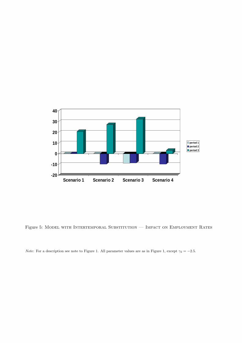
-20

-10

0

10

20

30

40

Scenario 1 Scenario 2 Scenario 3 Scenario 4

period 1period 2period 3

Figure 5: Model with Intertemporal Substitution — Impact on Employment Rates

Note: For a description see note to Figure 1. All parameter values are as in Figure 1, except γ2 = −2.5.

-20

-10

0

10

20

30

40

Scenario 1 Scenario 2 Scenario 3 Scenario 4

period 1period 2period 3

Figure 6: Model with Saving — Impact on Employment Rates

Note: For a description see note to Figure 1.

0

25

50

75

100

In-w

ork

bene

fit (

£/w

eek)

0 10 20 30 40 5016Hours per week

FC WFTCWFTC (childcare benefit as under FC)

With childcare benefit(a) FC and WFTC schedules, weekly awards

50

150

250

Dis

posa

ble

inco

me

(£/w

eek)

0 10 20 30 40 5016Hours per week

FC WFTCWFTC (childcare benefit as under FC)

With childcare benefit(b) Budget constraints under FC and WFTC

Figure 7: FC and WFTC Schedules and Budget Constraints

.636

.415

.2

.4

.6

.8P

ropo

rtio

n1999

1991 1993 1995 1997 1999 2001Year

single childless lone mothers

(a) Working 16+ hours per week

.636

.415

.2

.4

.6

.8

Pro

port

ion

1999

1991 1993 1995 1997 1999 2001Year

single childless lone, kid 0-4lone, kid 5-10 lone, kid 11-18

(Proportions for lone mothers are by age group of youngest child)(b) Working 16+ hours per week

Figure 8: Trends in Eligible Employment

.35

.4

.45

.5

.5

.55

.6

.65

.633

Pro

port

ion

Mar98

Sep97 Dec97 Mar98 Jun98 Sep98 Dec98

single childless lone mothers

(September 1997 - December 1998)(a) Monthly employment rates

.063

0

.03

.06

.09

.12

Pro

port

ion

Mar98

Sep97 Dec97 Mar98 Jun98 Sep98 Dec98Month/Year when New Job Started

single childless lone mothers

(Jobs started between September 1997 and December 1998)(b) Timing of new jobs

Figure 9: Employment Rates and Entry into New Jobs Around the AnnouncementDate