anatomy of market timing with moving averages€¦ · anatomy of market timing with moving averages...
TRANSCRIPT

Anatomy of Market Timing with Moving Averages∗
Valeriy Zakamulin†
This revision: August 26, 2015
Abstract
The underlying concept behind the technical trading indicators based on moving aver-ages of prices has remained unaltered for more than half of a century. The developmentin this field has consisted in proposing new ad-hoc rules and using more elaborate types ofmoving averages in the existing rules, without any deeper analysis of commonalities anddifferences between miscellaneous choices for trading rules and moving averages. In thispaper we uncover the anatomy of market timing rules with moving averages. Our analysisoffers a new and very insightful reinterpretation of the existing rules and demonstratesthat the computation of every trading indicator can equivalently be interpreted as thecomputation of the weighted moving average of price changes. This knowledge enables atrader to clearly understand the response characteristics of trading indicators and simplifydramatically the search for the best trading rule. As a straightforward application of theuseful knowledge revealed by our analysis, in this paper we also entertain a method offinding the most robust moving average weighting scheme. The method is illustrated usingthe long-run historical data on the Standard and Poor’s Composite stock price index. Wefind the most robust moving average weighting scheme and demonstrates its advantages.
Key words: technical analysis, market timing, momentum rule, price minus movingaverage rule, moving average change of direction rule, double crossover method, robustmoving average
JEL classification: G11, G17.
∗The author is grateful to an anonymous referee, Steen Koekebakker, Pete Nikolai, and the participants ofthe 3rd Economics & Finance Conference (Rome, Italy) for their insightful comments. The usual disclaimerapplies.
†a.k.a. Valeri Zakamouline, School of Business and Law, University of Agder, Service Box 422, 4604 Kris-tiansand, Norway, Tel.: (+47) 38 14 10 39, E-mail: [email protected]
1

1 Introduction
Technical analysis represents a methodology of forecasting the future price movements through
the study of past price data and uncovering some recurrent regularities, or patterns, in price
dynamics. One of the fundamental principles of technical analysis is that prices move in
trends. Analysts firmly believe that these trends can be identified in a timely manner and
used to generate profits and limit losses. Market timing is an active trading strategy that
implements this idea in practice. Specifically, this strategy is based on switching between the
market and cash depending on whether the prices trend upward or downward. A moving
average of prices is one of the oldest and most popular tools used in technical analysis for
detecting a trend. Over the past two decades, market timing with moving averages has been
the subject of substantial interest on the part of academics1 and investors alike.
However, despite a series of publications in academic journals, the market timing rules based
on moving averages have remained virtually unaltered for more than half of a century. Modern
technical analysis still remains art rather than science. The situation with market timing is as
follows. There have been proposed many technical trading rules based on moving averages of
prices calculated on a fixed size data window. The main examples are: the momentum rule,
the price-minus-moving-average rule, the change-of-direction rule, and the double-crossover
method. In addition, there are several popular types of moving averages: simple (or equally-
weighted) moving average, linearly-weighted moving average, exponentially-weighed moving
average, etc. As a result, there exists a large number of potential combinations of trading rules
with moving average weighting schemes. One of the controversies about market timing is over
which trading rule in combination with which moving average weighting scheme produces the
best performance. The situation is further complicated because in order to compute a moving
average one must define the size of the averaging window. Again, there is a big controversy
over the optimal size of this window.
There is a simple explanation for the existing situation with market timing. First of all,
technical traders do not really understand the response characteristics of the trading indicators2
1Some examples are: Brock, Lakonishok, and LeBaron (1992), Sullivan, Timmermann, and White (1999),Okunev and White (2003), Faber (2007), Gwilym, Clare, Seaton, and Thomas (2010), Moskowitz, Ooi, andPedersen (2012), Kilgallen (2012), Clare, Seaton, Smith, and Thomas (2013), Zakamulin (2014), Glabadanidis(2015).
2In our definition, a “trading indicator” denotes an equation (or a formula) that specifies how the technicaltrading signal is computed using the prices in the averaging window.
2

they use. The selection of the combination of a trading rule with a moving average weighting
scheme is made based mainly on intuition rather than any deeper analysis of commonalities
and differences between miscellaneous choices for trading rules and moving average weighting
schemes. The development in this field has consisted in proposing new ad-hoc rules and using
more elaborate types of moving averages (for example, moving averages of moving averages)
in the existing rules.
The main contribution of this paper is to uncover the anatomy of market timing rules
with moving averages of prices. Specifically, we present a methodology for examining how
the value of a trading indicator is computed. Then using this methodology we study the
computation of trading indicators in many market timing rules and analyze the commonalities
and differences between the rules. We reveal that despite being computed seemingly different
at the first sight, all technical trading indicators considered in this paper are computed in
the same general manner. In particular, the computation of every technical trading indicator
can equivalently be interpreted as the computation of a weighted moving average of price
changes. Consequently, the only real difference, between diverse market timing rules coupled
with various types of moving averages, lies in the weighting scheme used to compute the moving
average of price changes.
Our methodology of analyzing the computation of trading indicators for the timing rules
based on moving averages offers a broad and clear perspective on the relationship between
different rules. We show, for example, that every trading rule can also be presented as a
weighted average of the momentum rules computed using different averaging periods. Thus,
the momentum rule might be considered as an elementary trading rule on the basis of which
one can construct more elaborate rules. In addition, we establish a one-to-one equivalence
between a price-minus-moving-average rule and a corresponding moving-average-change-of-
direction rule. Overall, our analysis offers a new and very insightful re-interpretation of the
existing market timing rules.
The second contribution of this paper is a straightforward application of the useful knowl-
edge revealed by our analysis of timing rules based on moving averages of prices. Previously, in
order to select the best combination of a trading rule with a moving average weighting scheme
and a size of the averaging window, using relevant historical data a trader had to perform
the test of all possible combinations in order to find the combination with the best observed
3

performance in a back test.3 Our result allows a trader to simplify dramatically this procedure
because one needs only to test various combinations of weighting schemes (used to compute
the moving average of price changes) and averaging periods. Yet, we argue that this procedure
to selecting the best trading combination has two potentially very serious flaws. In particu-
lar, we find that there is no single optimal size of the averaging window.4 On the contrary,
empirical evidence suggests that there are substantial time-variations in the optimal size of
the averaging window for each weighting scheme. In addition, Zakamulin (2014) demonstrated
that the performance of a market timing strategy, relative to that of its passive counterpart,
is highly uneven over time. Therefore, the issue of outliers is of concern. This is because in
the presence of outliers (extraordinary good or bad performance over a rather short historical
period) the long-run performance of a trading combination does not reflect its typical per-
formance over short and medium runs. As a result of these two issues, the best performing
trading combination in the past might not perform well in the near future.
We entertain a novel approach to selecting the trading rule (specified by a particular moving
average weighting scheme) to use for the purpose of timing the market. The motivation for this
approach is twofold. First, we acknowledge that there is no single optimal size of the averaging
window. Second, we acknowledge that the performance of a trading rule is highly uneven
through time and over some relatively short particular historical episodes the performance
might be unusually far from that over the rest of the dataset. Based on these premises, we find
the most robust moving average weighting scheme. By robustness of a weighting scheme we
mean not only its robustness to outliers. Robustness of a weighting scheme is also defined as
its ability to generate sustainable performance under all possible market scenarios regardless
of the size of the averaging window. Our approach is illustrated using the long-run historical
data on the Standard and Poor’s Composite stock price index.
The rest of the paper is organized as follows. In the subsequent Section 2 we present the
moving averages and trading rules considered in the paper. Then in Section 3 we demonstrate
the anatomy of trading rules with different moving averages. Section 4 describes our method-
ology for finding a robust moving average, presents the most robust moving average weighting
3Even though this approach to selecting the best trading combination is termed as “data-mining”, thisapproach works and the only real issue with this approach is that it systematically overestimates how well thetrading combination will perform in the future (Aronson (2006), Zakamulin (2014)).
4To shorten the paper, these results are not reported.
4

scheme, and demonstrates its advantages. Finally, Section 5 concludes the paper.
2 Moving Averages and Technical Trading Rules
2.1 Moving Averages
A moving average of prices is calculated using a fixed size data “window” that is rolled through
time. The length of this window of data, also called the lookback period or averaging period, is
the time interval over which the moving average is computed. We follow the standard practice
and use prices, not adjusted for dividends, in the computation of moving averages and all
technical trading indicators. More formally, let (P1, P2, . . . , PT ) be the observations of the
monthly5 closing prices of a stock price index. A moving average at time t is computed using
the last closing price Pt and k lagged prices Pt−j , j ∈ [1, k]. It is worth noting that the time
interval over which the moving average is computed amounts to k months and includes k + 1
monthly observations. Generally, each price observation in the rolling window of data has
its own weight in the computation of a moving average. More formally, a weighted Moving
Average at month-end t with k lagged prices (denoted by MAt(k)) is computed as
MAt(k) =wtPt + wt−1Pt−1 + wt−2Pt−2 + . . .+ wt−kPt−k
wt + wt−1 + wt−2 + . . .+ wt−k=
∑kj=0wt−jPt−j∑k
j=0wt−j
, (1)
where wt−j is the weight of price Pt−j in the computation of the weighted moving average.
It is worth observing that in order to compute a moving average one has to use at least one
lagged price, this means that one should have k ≥ 1. Note that when the number of lagged
prices is zero, a moving average becomes the last closing price, that is, MAt(0) = Pt.
The most commonly used types of moving averages are: the Simple Moving Average (SMA),
the Linear (or linearly weighted) Moving Average (LMA), and the Exponential Moving Average
(EMA). A less commonly used type of moving average is the Reverse Exponential Moving
5Throughout the paper, we assume that the price data comes at the monthly frequency. Yet the resultspresented in the first part of the paper are valid for any data frequency.
5

Average (REMA). These moving averages at month-end t are computed as
SMAt(k) =1
k + 1
k∑j=0
Pt−j , LMAt(k) =
∑kj=0(k − j + 1)Pt−j∑k
j=0(k − j + 1),
EMAt(k) =
∑kj=0 λ
jPt−j∑kj=0 λ
j, REMAt(k) =
∑kj=0 λ
k−jPt−j∑kj=0 λ
k−j,
(2)
where 0 < λ ≤ 1 is a decay factor.
As compared with the simple moving average, either the linearly weighted moving average
or the exponentially weighted moving average puts more weight on the more recent price ob-
servations. The usual justification for the use of these types of moving averages is a widespread
belief that the most recent stock prices contain more relevant information on the future direc-
tion of the stock price than earlier stock prices. In the linearly weighted moving average the
weights decrease in arithmetic progression. In particular, in LMA(k) the latest observation
has weight k+1, the second latest k, etc. down to one. A disadvantage of the linearly weighted
moving average is that the weighting scheme is too rigid. In contrast, by varying the value of
λ in the exponentially weighted moving average, one is able to adjust the weighting to give
greater or lesser weight to the most recent price. The properties of the exponential moving
average:
limλ→1
EMAt(k) = SMAt(k), limλ→0
EMAt(k) = Pt. (3)
Contrary to the normal exponential moving average that gives greater weights to the most
recent prices, the reverse exponential moving average assigns greater weights to the most oldest
prices and decreases the importance of the most recent prices. The properties of the reverse
exponential moving average:
limλ→1
REMAt(k) = SMAt(k), limλ→0
REMAt(k) = Pt−k. (4)
Instead of the regular moving averages of prices considered above, traders sometimes use
more elaborate moving averages that can be considered as “moving averages of moving aver-
ages”. Specifically, instead of using a regular moving average to smooth the price series, some
traders perform either double- or triple-smoothing of the price series. The main examples
of this type of moving averages are: Triangular Moving Average, Double Exponential Moving
6

Average, and Triple Exponential Moving Average (see, for example, Kirkpatrick and Dahlquist
(2010)). To shorten and streamline the presentation, we will not consider these moving aver-
ages in our paper. Yet our methodology can be applied to the analysis of the trading indicators
based on this type of moving averages in a straightforward manner.
2.2 Technical Trading Rules
Every market timing rule prescribes investing in the stocks (that is, the market) when a Buy
signal is generated and moving to cash or shorting the market when a Sell signal is generated.
In the absence of transaction costs, the time t return to a market timing strategy is given by
rt = δt|t−1rMt +(1− δt|t−1
)rft, (5)
where rMt and rft are the month t returns on the stock market (including dividends) and the
risk-free asset respectively, and δt|t−1 ∈ {0, 1} is a trading signal for month t (0 means Sell and
1 means Buy) generated at the end of month t− 1.
In each market timing rule the generation of a trading signal is a two-step process. At the
first step, one computes the value of a technical trading indicator using the last closing price
and k lagged prices
IndicatorTR(k)t = Eq(Pt, Pt−1, . . . , Pt−k), (6)
where TR denotes the timing rule and Eq(·) is the equation that specifies how the technical
trading indicator is computed. At the second step, using a specific function one translates the
value of the technical indicator into the trading signal. In all market timing rules considered
in this paper, the Buy signal is generated when the value of a technical trading indicator is
positive. Otherwise, the Sell signal is generated. Thus, the generation of a trading signal can
be interpreted as an application of the following (mathematical) indicator function to the value
of the technical indicator
δt+1|t = 1+
(Indicator
TR(k)t
), (7)
7

where the indicator function 1+(·) is defined by
1+(x) =
1 if x > 0,
0 if x ≤ 0.
(8)
We start the presentation of trading rules considered in the paper with the Momentum rule
(MOM) which is the simplest and most basic market timing rule. In the Momentum rule one
compares the last closing price, Pt, with the closing price k months ago, Pt−k. In this rule a
Buy signal is generated when the last closing price is greater than the closing price k months
ago. Formally, the technical trading indicator for the Momentum rule is computed as
IndicatorMOM(k)t = MOMt(k) = Pt − Pt−k. (9)
Then the trading signal is generated by
δMOM(k)t+1|t = 1+ (MOMt(k)) . (10)
Most often, in order to generate a trading signal, a trader compares the last closing price
with the value of a k-month moving average. In this case a Buy signal is generated when the
last closing price is above a k-month moving average. Otherwise, if the last closing price is
below a k-month moving average, a Sell signal is generated. Formally, the technical trading
indicator for the Price-Minus-Moving-Average rule (P-MA) is computed as
IndicatorP-MA(k)t = Pt −MAt(k). (11)
Some traders argue that the price is noisy and the Price-Minus-Moving-Average rule pro-
duces many false signals (whipsaws). They suggest to address this problem by employing two
moving averages in the generation of a trading signal: one shorter average with averaging pe-
riod s and one longer average with averaging period k > s. This technique is called the Double
8

Crossover Method6 (DCM). In this case the technical trading indicator is computed as
IndicatorDCM(s,k)t = MAt(s)−MAt(k). (12)
It is worth noting the obvious relationship
IndicatorDCM(0,k)t = Indicator
P-MA(k)t . (13)
Less often, in order to generate a trading signal, the traders compare the most recent value
of a k-month moving average with the value of a k-month moving average in the preceding
month. Intuitively, when the stock prices are trending upward (downward) the moving average
is increasing (decreasing). Consequently, in this case a Buy signal is generated when the value of
a k-month moving average has increased over a month. Otherwise, a Sell signal is generated.
Formally, the technical trading indicator for the Moving-Average-Change-of-Direction rule
(∆MA) is computed as
Indicator∆MA(k)t = MAt(k)−MAt−1(k). (14)
3 Anatomy of Trading Rules
3.1 Preliminaries
It has been known for years that there is a relationship between the Momentum rule and the
Simple-Moving-Average-Change-of-Direction rule.7 In particular, note that
SMAt(k − 1)− SMAt−1(k − 1) =Pt − Pt−k
k=
MOMt(k)
k. (15)
Therefore
Indicator∆SMA(k−1)t ≡ Indicator
MOM(k)t , (16)
where the symbol “≡” means equivalence. The equivalence of two technical indicators stems
from the following property: the multiplication of a technical indicator by any positive real num-
6Also known as the Moving Average Crossover.7See, for example, http://en.wikipedia.org/wiki/Momentum (technical analysis).
9

ber produces an equivalent technical indicator. This is because the trading signal is generated
depending on the sign of the technical indicator. The formal presentation of this property:
1+ (a× Indicatort(k)) = 1+ (Indicatort(k)) , (17)
where a is any positive real number. Using relation (16) as an illustrating example, observe
that if SMAt(k−1)−SMAt−1(k−1) > 0 then MOMt(k) > 0 and vice versa. In other words,
the Simple-Moving-Average-Change-of-Direction rule, ∆SMA(k− 1), generates the Buy (Sell)
trading signal when the Momentum rule, MOMt(k), generates the Buy (Sell) trading signal.
What else can we say about the relationship between different market timing rules? The
ultimate goal of this section is to answer this question and demonstrate that all market timing
rules considered in this paper are closely interconnected. In particular, we are going to show
that the computation of a technical trading indicator for every market timing rule can be
interpreted as the computation of the weighted moving average of monthly price changes over
the averaging period. We will do it sequentially for each trading rule.
3.2 Momentum Rule
The computation of the technical trading indicator for the Momentum rule can equivalently
be represented by
IndicatorMOM(k)t = MOMt(k) = Pt − Pt−k
= (Pt − Pt−1) + (Pt−1 − Pt−2) + ...+ (Pt−k+1 − Pt−k) =
k∑i=1
∆Pt−i,(18)
where ∆Pt−i = Pt−i+1−Pt−i denotes the monthly price change. Consequently, using property
(17), the computation of the technical indicator for the Momentum rule is equivalent to the
computation of the equally weighted moving average of the monthly price changes:
IndicatorMOM(k)t ≡ 1
k
k∑i=1
∆Pt−i. (19)
10

3.3 Price-Minus-Moving-Average Rule
First, we derive the relationship between the Price-Minus-Moving-Average rule and the Mo-
mentum rule:
IndicatorP-MA(k)t = Pt −MAt(k) = Pt −
∑kj=0wt−jPt−j∑k
j=0wt−j
=
∑kj=0wt−jPt −
∑kj=0wt−jPt−j∑k
j=0wt−j
=
∑kj=1wt−j(Pt − Pt−j)∑k
j=0wt−j
=
∑kj=1wt−jMOMt(j)∑k
j=0wt−j
.
(20)
Using property (17), the relation above can be conveniently re-written as
IndicatorP-MA(k)t ≡
∑kj=1wt−jMOMt(j)∑k
j=1wt−j
. (21)
Consequently, the computation of the technical indicator for the Price-Minus-Moving-Average
rule, Pt−MAt(k), is equivalent to the computation of the weighted moving average of technical
indicators for the Momentum rules, MOMt(j), for j ∈ [1, k]. It is worth noting that the
weighting scheme for computing the moving average of the momentum technical indicators,
MOMt(j), is the same as the weighting scheme for computing the weighted moving average
MAt(k).
Second, we use identity (18) and rewrite the numerator in (21) as
k∑j=1
wt−jMOMt(j) =
k∑j=1
wt−j
j∑i=1
∆Pt−i = wt−1∆Pt−1 + wt−2(∆Pt−1 +∆Pt−2) + . . .
+ wt−k(∆Pt−1 +∆Pt−2 + . . .+∆Pt−k) = (wt−1 + . . .+ wt−k)∆Pt−1
+ (wt−2 + . . .+ wt−k)∆Pt−2 + . . .+ wt−k∆Pt−k =
k∑i=1
k∑j=i
wt−j
∆Pt−i.
(22)
The last expression tells us that the numerator in (21) is a weighted sum of the monthly
price changes over the averaging window, where the weight of ∆Pt−i equals∑k
j=iwt−i. Thus,
another alternative expression for the computation of the technical indicator for the Price-
11

Minus-Moving-Average rule is given by
IndicatorP-MA(k)t ≡
∑ki=1
(∑kj=iwt−j
)∆Pt−i∑k
i=1
(∑kj=iwt−j
) =
∑ki=1 xt−i∆Pt−i∑k
i=1 xt−i
. (23)
where
xt−i =k∑
j=i
wt−j (24)
is the weight of the price change ∆Pt−i. In words, the computation of the technical indicator
for the Price-Minus-Moving-Average rule is equivalent to the computation of the weighted
moving average of the monthly price changes in the averaging window.
It is important to note from equation (24) that the application of the Price-Minus-Moving-
Average rule usually leads to overweighting the most recent price changes as compared to the
original weighting scheme used to compute the moving average of prices. If the weighting
scheme in a trading rule is already designed to overweight the most recent prices, then as a
rule the trading signal is computed with a much stronger overweighting the most recent price
changes. This will be demonstrated below.
Let us now, on the basis of (23), present the alternative expressions for the computation
of Price-Minus-Moving-Average technical indicators that use the specific weighting schemes
described in the preceding section. We start with the Simple Moving Average which uses the
equally weighted moving average of prices. In this case the weight of ∆Pt−i is given by
xt−i =
k∑j=i
wt−j =
k∑j=i
1 = k − i+ 1. (25)
Consequently, the equivalent representation for the computation of the technical indicator for
the Price-Minus-Simple-Moving-Average rule:
IndicatorP-SMA(k)t ≡
∑ki=1(k − i+ 1)∆Pt−i∑k
i=1(k − i+ 1)=
k∆Pt−1 + (k − 1)∆Pt−2 + . . .+∆Pt−k
k + (k − 1) + . . .+ 1. (26)
This suggests that alternatively we can interpret the computation of the technical indicator
for the Price-Minus-Simple-Moving-Average rule as the computation of the linearly weighted
moving average of monthly price changes.
12

We next consider the Linear Moving Average which uses the linearly weighted moving
average or prices. In this case the weight of ∆Pt−i is given by
xt−i =
k∑j=i
wt−j =
k∑j=i
(k − j + 1) =(k − i+ 1)(k − i+ 2)
2, (27)
which is the sum of the terms of arithmetic sequence from 1 to k − i + 1 with the common
difference of 1. As the result, the equivalent representation for the computation of the technical
indicator for the Price-Minus-Linear-Moving-Average rule
IndicatorP-LMA(k)t ≡
∑ki=1
(k−i+1)(k−i+2)2 ∆Pt−i∑k
i=1(k−i+1)(k−i+2)
2
. (28)
Then we consider the Exponential Moving Average which uses the exponentially weighted
moving average or prices. In this case the weight of ∆Pt−i is given by
xt−i =k∑
j=i
wt−j =k∑
j=i
λj =λ
1− λ
(λi−1 − λk
), (29)
which is the sum of the terms of geometric sequence from λi to λk. Consequently, the equivalent
presentation for the computation of the technical indicator for the Price-Minus-Exponential-
Moving-Average rule
IndicatorP-EMA(k)t ≡
∑ki=1
(λi−1 − λk
)∆Pt−i∑k
i=1 (λi−1 − λk)
. (30)
If k is relatively large such that λk ≈ 0, then the expression for the computation of the technical
indicator for the Price-Minus-Exponential-Moving-Average rule becomes
IndicatorP-EMA(k)t ≡
∑ki=1 λ
i−1∆Pt−i∑ki=1 λ
i−1=
∆Pt−1 + λ∆Pt−2 + . . .+ λk−1∆Pt−k
1 + λ+ . . .+ λk−1, when λk ≈ 0.
(31)
In words, the computation of the trading signal for the Price-Minus-Exponential-Moving-
Average rule, when k is rather large, is equivalent to the computation of the exponential
moving average of monthly price changes. It is worth noting that this is probably the only
trading rule where the weighting scheme for the computation of moving average of prices is
identical to the weighting scheme for the computation of moving average of price changes.
13

The weight of ∆Pt−i for the Reverse Exponential Moving Average is given by
xt−i =
k∑j=i
wt−j =
k∑j=i
λk−j =1− λk−i+1
1− λ, (32)
which is the sum of the terms of geometric sequence from 1 to λk−i. Consequently, the
equivalent representation for the computation of the technical indicator for the Price-Minus-
Reverse-Exponential-Moving-Average rule
IndicatorP-REMA(k)t ≡
∑ki=1
(1− λk−i+1
)∆Pt−i∑k
i=1 (1− λk−i+1). (33)
3.4 Moving-Average-Change-of-Direction Rule
The value of this technical trading indicator is based on the difference of two weighted moving
averages computed at times t and t− 1 respectively. We assume that the size of the averaging
window is k − 1 months, the reason for this assumption will become clear very soon. The
straightforward computation yields
Indicator∆MA(k − 1)t = MAt(k − 1)−MAt−1(k − 1) =
∑k−1i=0 wt−iPt−i∑k−1
i=0 wt−i
−∑k−1
i=0 wt−iPt−i−1∑k−1i=0 wt−i
=
∑k−1i=0 wt−i (Pt−i − Pt−i−1)∑k−1
i=0 wt−i
=
∑ki=1wt−i+1∆Pt−i∑k
i=1wt−i+1
.
(34)
Consequently, the computation of the technical indicator for the Moving-Average-Change-of-
Direction rule can be directly interpreted as the computation of the weighted moving average
of monthly price changes:
Indicator∆MA(k − 1)t =
∑ki=1wt−i+1∆Pt−i∑k
i=1wt−i+1
. (35)
Note that the weighting scheme for the computation of the moving average of monthly price
changes is the same as for the computation of moving average of prices. From (35) we easily
recover the relationship for the case of the Simple Moving Average where wt−i+1 = 1 for all i
Indicator∆SMA(k − 1)t ≡
∑ki=1∆Pt−i
k≡ Indicator
MOM(k)t , (36)
14

where the last equivalence follows from (19).
In the case of the Linear Moving Average, where wt−i+1 = k − i + 1, we derive a new
relationship:
Indicator∆LMA(k − 1)t ≡
∑ki=1(k − i+ 1)∆Pt−i∑k
i=1(k − i+ 1)≡ IndicatorP-SMA
t (k), (37)
where the last equivalence follows from (26). Putting it into words, the Price-Minus-Simple-
Moving-Average rule, Pt−SMAt(k), prescribes investing in the stocks (moving to cash) when
the Linear Moving Average of prices over the averaging window of k − 1 months increases
(decreases).
In the case of the Exponential Moving Average and Reverse Exponential Moving Average,
the resulting expressions for the Change-of-Direction rules can be written as
Indicator∆EMA(k − 1)t =
∑ki=1 λ
i−1∆Pt−i∑ki=1 λ
i−1, (38)
Indicator∆REMA(k − 1)t =
∑ki=1 λ
k−i∆Pt−i∑ki=1 λ
k−i. (39)
Observe in particular that if k is rather large, then, using result (31), we obtain yet another
new relationship:
IndicatorP-EMA(k)t ≡ Indicator
∆EMA(k − 1)t , when λk ≈ 0. (40)
In words, when k is rather large, the Price-Minus-Exponential-Moving-Average rule is equiv-
alent to the Exponential-Moving-Average-Change-of-Direction rule. As it might be observed,
for the majority of weighting schemes considered in the paper, there is a one-to-one equivalence
between a Price-Minus-Moving-Average rule and a corresponding Moving-Average-Change-of-
Direction rule. Therefore, the majority of the moving-average-change-of-direction rules (and
may be all of them) can also be expressed as the moving average of Momentum rules.
Finally it is worth commenting that the traders had long ago taken notice of the fact that,
for example, very often a Buy signal is generated first by the Price-Minus-Moving-Average rule,
then with some delay a Buy signal is generated by the Moving-Average-Change-of-Direction
rule. Therefore the traders sometimes use the trading signal of the Moving-Average-Change-
15

of-Direction rule to “confirm” the signal of the Price-Minus-Moving-Average rule (see Murphy
(1999), Chapter 9). Our analysis provides a simple explanation for the existence of a delay
between the signals generated by these two rules. Specifically, the delay naturally occurs be-
cause the Price-Minus-Moving-Average rule overweights more heavily the most recent price
changes than the Moving-Average-Change-of-Direction rule computed using the same weight-
ing scheme. Therefore the Price-Minus-Moving-Average rule reacts more quickly to the recent
trend changes than the Moving-Average-Change-of-Direction rule.8
3.5 Double Crossover Method
The relationship between the Double Crossover Method and the Momentum rule is as follows
(here we use result (20))
IndicatorDCM(s, k)t = MAt(s)−MAt(k) = (Pt −MAt(k))− (Pt −MAt(s))
=
∑kj=1w
kt−jMOMt(j)∑kj=0w
kt−j
−∑s
j=1wst−jMOMt(j)∑sj=0w
st−j
.(41)
Different superscripts in the weights mean that for the same subscript the weights are generally
not equal. For example, in case of either linearly weighted moving averages or reverse expo-
nential moving averages wkt−j ̸= ws
t−j , yet for the other weighting schemes considered in this
paper wkt−j = ws
t−j . In order to get a closer insight into the anatomy of the Double Crossover
Method, we assume that one uses the exponential weighting scheme in the computation of
moving averages (as it most often happens in practice). In this case the expression for the
value of the technical indicator in terms of monthly price changes is given by (here we use
8Assume, for example, that the trader uses the simple moving average weighting scheme in both the rules. Inthis case our result says that the Price-Minus-Simple-Moving-Average rule is equivalent to the Linear-Moving-Average-Change-of-Direction rule. As a consequence, it is naturally to expect that the Price-Minus-Simple-Moving-Average rule reacts more quickly to the recent trend changes than the Simple-Moving-Average-Change-of-Direction rule.
16

results (22) and (29))
IndicatorDCM(s, k)t =
∑kj=1 λ
j∑j
i=1∆Pt−i∑kj=0 λ
j−
∑sj=1 λ
j∑j
i=1∆Pt−i∑sj=0 λ
j=
∑ki=1
(∑kj=i λ
j)∆Pt−i∑k
j=1 λj
−
∑si=1
(∑sj=i λ
j)∆Pt−i∑s
j=1 λj
=
∑ki=1
(λi − λk+1
)∆Pt−i
1− λk+1−
∑si=1
(λi − λs+1
)∆Pt−i
1− λs+1.
(42)
If we assume in addition that both s and k are relatively large such that λs ≈ 0 and λk ≈ 0,
then we obtain
IndicatorDCM(s, k)t ≈
k∑i=1
λi∆Pt−i −s∑
i=1
λi∆Pt−i =k∑
i=s+1
λi∆Pt−i. (43)
The expression above can be conveniently re-written as
IndicatorDCM(s, k)t ≡
∑ki=s+1 λ
i−s−1∆Pt−i∑kj=s+1 λ
i−s−1when k > s, λs ≈ 0, λk ≈ 0. (44)
In words, the computation of the trading signal for the Double Crossover Method based on
the exponentially weighted moving averages of lengths s and k > s, when both s and k are
rather large, is equivalent to the computation of the exponentially weighted moving average
of monthly price changes, ∆Pt−i, for i ∈ [s+ 1, k]. Note that the most recent s monthly price
changes completely disappear in the computation of the technical trading indicator. In other
words, in the computation of the trading indicator one disregards, or skips, the most recent
s monthly price changes. When the values of s and k are not rather large, the most recent
s monthly price changes do not disappear in the computation of the technical indicator, yet
the weights of these price changes are reduced as compared to the weight of the subsequent
(s+ 1)-th price change.
3.6 Discussion
Summing up the results presented above, all technical trading indicators considered in this
paper are computed in the same general manner. We find, for instance, that the computation
of every technical trading indicator can be interpreted as the computation of a weighted average
17

of the momentum rules computed using different averaging periods. Thus, the momentum rule
might be considered as an elementary trading rule on the basis of which one can construct
more elaborate rules. The most insightful conclusion emerging from our analysis is that the
computation of every technical trading indicator, based on moving averages of prices, can also
be interpreted as the computation of the weighted moving average of price changes.
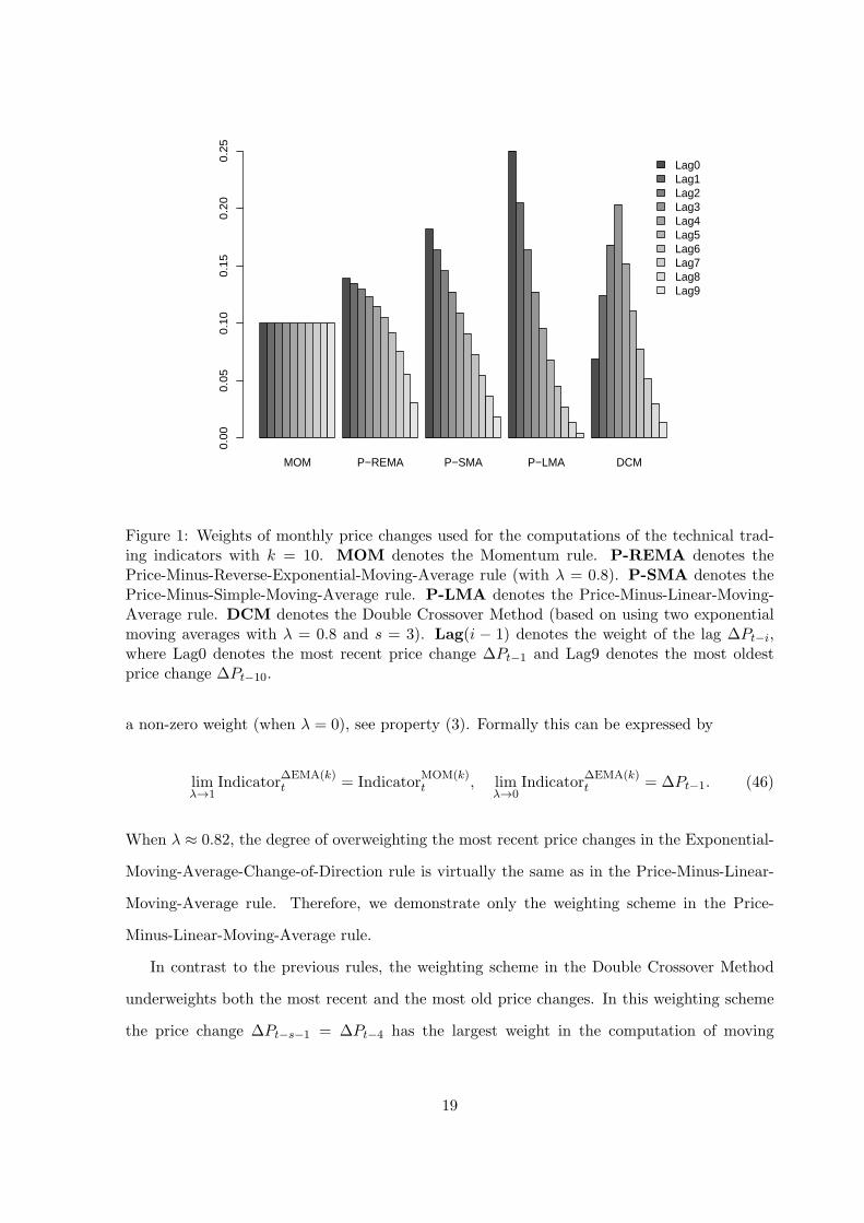
Our main conclusion is that, despite being computed seemingly different at the first sight,
the only real difference between miscellaneous rules lies in the weighting scheme used to com-
pute the moving average of price changes. Figure 1 illustrates a few distinctive weighting
schemes for the computation of technical trading indicators based on moving averages. In par-
ticular, this figure illustrates the weighting schemes for the Momentum rule, the Price-Minus-
Reverse-Exponential-Moving-Average rule (with λ = 0.8), the Price-Minus-Simple-Moving-
Average rule, the Price-Minus-Linear-Moving-Average rule, and the Double Crossover Method
(based on using two exponential moving averages with λ = 0.8). For all technical indicators
we use k = 10 which means that to compute the value of a technical indicator we use the most
recent price change, ∆Pt−1, denoted as Lag0, and 9 preceding lagged price changes up to lag
∆Pt−10, denoted as Lag9. In addition, in the computation of the technical indicator for the
Double Crossover Method we use s = 3.
Apparently, the Momentum rule assigns equal weights to all monthly price changes in the
averaging window. The next three rules overweight the most recent price changes. They are
arranged according to increasing degree of overweighting. Whereas the Price-Minus-Simple-
Moving-Average rule employs the linear weighting scheme, the degree of overweighting in the
Price-Minus-Reverse-Exponential-Moving-Average rule can be gradually varied from the equal
weighting scheme (when λ = 0) to the linear weighting scheme (when λ = 1), see property (4).
Formally this can be expressed by
limλ→0
IndicatorP-REMA(k)t = Indicator
MOM(k)t , lim
λ→1Indicator
P-REMA(k)t = Indicator
P-SMA(k)t .
(45)
Comparing to the Price-Minus-Simple-Moving-Average rule, a higher degree of overweight-
ing can be attained by using the Exponential-Moving-Average-Change-of-Direction rule. The
degree of overweighting in this rule can be gradually varied from the linear weighting scheme
(when λ = 1) to the very extreme overweighting where only the most recent price change has
18
MOM P−REMA P−SMA P−LMA DCM
Lag0Lag1Lag2Lag3Lag4Lag5Lag6Lag7Lag8Lag9
0.00
0.05
0.10
0.15
0.20
0.25
Figure 1: Weights of monthly price changes used for the computations of the technical trad-ing indicators with k = 10. MOM denotes the Momentum rule. P-REMA denotes thePrice-Minus-Reverse-Exponential-Moving-Average rule (with λ = 0.8). P-SMA denotes thePrice-Minus-Simple-Moving-Average rule. P-LMA denotes the Price-Minus-Linear-Moving-Average rule. DCM denotes the Double Crossover Method (based on using two exponentialmoving averages with λ = 0.8 and s = 3). Lag(i − 1) denotes the weight of the lag ∆Pt−i,where Lag0 denotes the most recent price change ∆Pt−1 and Lag9 denotes the most oldestprice change ∆Pt−10.
a non-zero weight (when λ = 0), see property (3). Formally this can be expressed by
limλ→1
Indicator∆EMA(k)t = Indicator
MOM(k)t , lim
λ→0Indicator
∆EMA(k)t = ∆Pt−1. (46)
When λ ≈ 0.82, the degree of overweighting the most recent price changes in the Exponential-
Moving-Average-Change-of-Direction rule is virtually the same as in the Price-Minus-Linear-
Moving-Average rule. Therefore, we demonstrate only the weighting scheme in the Price-
Minus-Linear-Moving-Average rule.
In contrast to the previous rules, the weighting scheme in the Double Crossover Method
underweights both the most recent and the most old price changes. In this weighting scheme
the price change ∆Pt−s−1 = ∆Pt−4 has the largest weight in the computation of moving
19

average.
Our alternative representation of the computation of technical trading indicators by means
of the moving average of price changes, together with the graphical visualization of the weight-
ing schemes for different rules presented in Figure 1, reveals a couple of paradoxes. The first
paradox consists in the following. Many traders argue that the most recent stock prices contain
more relevant information on the future direction of the stock price than earlier stock prices.
Therefore, one should better use the LMA(k) instead of the SMA(k) in the computation of
trading signals. Yet in terms of the monthly price changes the application of the Price-Minus-
Simple-Moving-Average rule already leads to overweighting the most recent price changes. If it
is the most recent stock price changes (but not prices) that contain more relevant information
on the future direction of the stock price, then the use of the Price-Minus-Linear-Moving-
Average rule leads to a severe overweighting the most recent price changes, which might be
suboptimal.
The other paradox is related to the effect produced by the use of a shorter moving average
in the computation of a trading signal for the Double Crossover Method. Specifically, our al-
ternative representation of the computation of technical trading indicators reveals an apparent
conflict of goals that some traders want to pursue. In particular, on the one hand, one wants
to put more weight on the most recent prices that are supposed to be more relevant. On the
other hand, one wants to smooth the noise by using a shorter moving average instead of the
last closing price (as in the Price-Minus-Moving-Average rule). It turns out that these two
goals cannot be attained simultaneously because the noise smoothing results in a substantial
reduction of weights assigned to the most recent price changes (and, therefore, most recent
prices). Figure 1 clearly demonstrates that the weighting scheme for the Double Crossover
Method has a hump-shaped form such that the largest weight is given to the monthly price
change at lag s. Then, as the lag number decreases to 0 or increases to k − 1, the weight of
the lag decreases. Consequently, the use of the Double Crossover Method can be justified only
when the price change at lag s contains the most relevant information on the future direction
of the stock price.
20

4 A Robust Moving Average Weighting Scheme
4.1 Data
In our applied study we use the capital appreciation and total return on the Standard and
Poor’s Composite stock price index, as well as the risk-free rate of return proxied by the
Treasury Bill rate. The sample period begins in January 1857, ends in December 2014, and
covers 158 full years (1896 monthly observations). The data on the S&P Composite index
comes from two sources. The returns for the period January 1857 to December 1925 are
provided by William Schwert.9 The returns for the period January 1926 to December 2014
are computed from the closing monthly priced of the S&P Composite index and corresponding
dividend data provided by Amit Goyal.10 The Treasury Bill rate for the period January 1920
to December 2014 is also provided by Amit Goyal. Because there was no risk-free short-term
debt prior to the 1920s, we estimate it in the same manner as in Welch and Goyal (2008) using
the monthly data for the Commercial Paper Rates for New York. These data are available for
the period January 1857 to December 1971 from the National Bureau of Economic Research
(NBER) Macrohistory database.11 First, we run a regression
Treasury-bill ratet = α+ β × Commercial Paper Ratet + et (47)
over the period from January 1920 to December 1971. The estimated regression coefficients
are α = −0.00039 and β = 0.9156; the goodness of fit, as measured by the regression R-square,
amounts to 95.7%. Then the values of the Treasury Bill rate over the period January 1857 to
December 1919 are obtained using the regression above with the estimated coefficients for the
period 1920 to 1971.
4.2 The Methodology for Finding a Robust Moving Average
We say that a moving average weighting scheme is robust if it is able to generate sustainable
performance under all possible market scenarios regardless of the size of the averaging window.
Consequently, in order to find a robust weighting scheme, we need to evaluate the performances
9http://schwert.ssb.rochester.edu/data.htm10http://www.hec.unil.ch/agoyal/11http://research.stlouisfed.org/fred2/series/M13002US35620M156NNBR
21

of all different trading rules (where each rule is specified by a particular shape of the weighting
scheme), using all feasible sizes of the averaging window, and over all possible market scenarios.
Then we need to compare the performances and select a trading rule with the most stable
performance.
By performance we mean a risk-adjusted performance. Our measure of performance is the
Sharpe ratio which is a reward-to-total-risk performance measure. We compute the Sharpe
ratio using the methodology presented in Sharpe (1994). Specifically, the computation of the
Sharpe ratio starts with computing the excess returns, Rt = rt − rft, where rt is the period
t return to the market timing strategy given by equation (5), and rft is the period t risk-free
rate of return. Then the Sharpe ratio is computed as the ratio of the mean excess returns to
the standard deviation of excess returns. Because the Sharpe ratio is often criticized on the
grounds that the standard deviation appears to be an inadequate measure of risk, we also use
the Sortino ratio (due to Sortino and Price (1994)) as an alternative performance measure to
check the robustness of our findings.
In practice, the most typical recommended size of the averaging window amounts to 10-12
months (see, among others, Brock et al. (1992), Faber (2007), Moskowitz et al. (2012), and
Clare et al. (2013)). However, empirical evidence suggests that there are large time-variations
in the optimal size of the averaging window for each trading rule. Therefore, we require that
a robust moving average weighting scheme must generate a sustainable performance over a
broader manifold of horizons, from 4 to 18 months. That is, to find a robust moving average
we vary k ∈ [4, 18]. Note that the number of alternative sizes of the averaging window amounts
to m = 15.
Technical analysis is based on a firm belief that there are recurrent regularities, or patterns,
in the stock price dynamics. In other words, “history repeats itself”. Based on the paradigm
of historic recurrence, we expect that in the subsequent future time period the stock price
dynamics (one possible market scenario) will represent a repetition of already observed stock
price dynamics over a past period of the same length.12 The problem is that we do not know
12It is worth noting that very popular nowadays block-bootstrap methods of resampling the historical dataare based on the same historic recurrence paradigm. Specifically, block-bootstrap is a non-parametric methodof simulating alternative historical realizations of the underlying data series that are supposed to preserve allrelevant statistical properties of the original data series. In this method the simulated data series are generatedusing blocks of historical data. For a review of bootstrapping methods, see Berkowitz and Kilian (2000). Block-bootstrap is now widely used to draw statistical inference on the performance of active trading strategies (see,for example, Sullivan et al. (1999)).
22

what part of the history will repeat in the nearest future. Therefore we want that a robust
moving average weighting scheme generates a sustainable performance over all possible histor-
ical realizations of the stock price dynamics. We follow the most natural and straightforward
idea and split the total sample of historical data into n smaller blocks of data. These blocks
of historical data are considered as possible variants of the future stock price dynamics.
We need to make a choice of a suitable block length that should preferably include at least
one bear market. Our choice is to use the block length of l = 120 months (10 years) and is
partly motivated by the results reported by Pagan and Sossounov (2003). In particular, these
authors analyzed the properties of bull and bear markets using virtually the same dataset as
ours. The mean durations of the bull and bear markets are found to be 25 and 15 months
respectively. Therefore with the block length of 10 years we are almost guaranteed to cover a
few alternating bull and bear markets. In order to increase the number of blocks of data and
to decrease the performance dependence on the choice of the split points between the blocks
of data, we use 10-year blocks with a 5-year overlap between the blocks. Specifically, the first
block of data covers the 10-year period from January 1860 to December 1869; the second block
of data covers the 10-year period from January 1865 to December 1874; etc. As a result of this
partition, the number of 10-year blocks amounts to n = 30.
The generation of different shapes of the moving average weighting scheme is based on
the following idea. Even though there are various trading rules based on moving averages of
prices and various types of moving averages, there are basically only three types of the shape of
weighting scheme: equal weighting of price changes (as in the MOM rule), underweighting the
most old price changes (as in the P-MA rule or in the most ∆MA rules), and underweighting
both the most recent and the most old price changes (as in the DCM). In order to generate
these shapes, we will employ three types of weighting schemes based on exponential moving
averages: (1) convex EMA weighting scheme produced by ∆EMA(k) trading rule, (2) concave
EMA weighting scheme produced by P-REMA(k) trading rule, and (3) hump-shaped EMA
weighting scheme produced by DCM(s, k). There is an uncertainly about the proper choice
of the size of the shorter window s in the DCM rule. Since the most popular combination in
practice is to use a 200-day long window and a 50-day short window, we set s = 14k for all
values of k.
For some fixed number of price change lags k, the shape of each moving average weighting
23

0.00
0.05
0.10
0.15
0.20
0 1 2 3 4 5 6 7 8 9 10 11 12 13 14 15 16 17Lag
Weig
ht
Decay, λ
0.8
0.9
0.00
0.02
0.04
0.06
0.08
0 1 2 3 4 5 6 7 8 9 10 11 12 13 14 15 16 17Lag
Weig
ht
Decay, λ
0.6
0.9
Panel A: Convex EMA weighting scheme Panel B: Concave EMA weighting scheme
0.00
0.05
0.10
0.15
0 1 2 3 4 5 6 7 8 9 10 11 12 13 14 15 16 17Lag
Weig
ht
Decay, λ
0.7
0.9
Panel C: Hump-shaped EMA weighting scheme
Figure 2: The types of the moving average weighting schemes used for finding a robust movingaverage. Panel A illustrates the convex exponential moving average weighting scheme pro-duced by ∆EMA(k) trading rule. Panel B illustrates the concave exponential moving averageweighting scheme produced by P-REMA(k) trading rule. Panel C illustrates the hump-shapedexponential moving average weighting scheme produced by DCM(s, k) trading rule. λ denotesthe decay factor. In all illustrations the number of price changes k = 18. Lag denotes theweight of the lag ∆Pt−i, where Lag0 denotes the most recent price change ∆Pt−1 and Lag17denotes the most oldest price change ∆Pt−18.
scheme depends on the value of the decay factor λ. In order to generates many different shapes
of the weighting function, in each trading rule we vary the value of λ ∈ {0.00, 0.99} with a step
of ∆λ = 0.01. As a result, for each type of the EMA we get 100 different shapes. Since we
have three different types of the EMA, the total number of generated shapes amounts to 300.
As a result, we obtain 300 different trading strategies; each strategy is specified by a particular
shape of the moving average weighting scheme. Figure 2 illustrates the shapes of each type
of weighting schemes for two arbitrary values of λ. Both convex and concave EMA weighting
schemes underweight the most old price changes. Yet, whereas in the convex EMA the weight
of the price lag i is a convex exponential function with respect to i (see equation (38)), in the
concave EMA the weight of the price lag i is a concave exponential function with respect to i
24

(see equation (33)). It is worth repeating (recall the discussion in Section 3.6) that by varying
the value of λ from 0 to 1, the weighting scheme of the concave EMA varies from the equal
weighting scheme to the linear weighting scheme; the weighting scheme of the convex EMA
varies from the very extreme overweighting (where only the most recent price change has a
non-zero weight) to the linear weighting scheme.
The choice of the most robust moving average weighting scheme is made using the following
method. We fix the size of the averaging window and simulate all trading strategies over the
total sample. Subsequently, we measure and record the performance of every moving average
weighting scheme over each block of data. In each block of data, we then rank the performances
of all alternative moving average weighting schemes. In particular, the weighting scheme with
the best performance in a block of data is assigned rank 1 (highest), the one with the next best
performance is assigned rank 2, and then down to rank 300 (lowest). After that, we change
the size of the averaging window, k, and repeat the procedure all over again. In the end, each
moving average weighting scheme receives n× k = 30× 15 = 450 ranks; each of these ranks is
associated with the weighting scheme’s performance for some specific block of data and some
specific size of the averaging window. Finally we compute the median rank for each moving
average weighting scheme. We assume that the most robust moving average weighting scheme
has the highest median rank. That is, the most robust moving average weighting scheme is
that one that has the highest median performance rank across different historical sub-periods
and different sizes of the averaging window. Note that since we use the median rank instead
of the average rank, and since we use ranks instead of performances, we avoid the outliers
issue (when an extraordinary good performance in some specific historical period influences
the overall performance).
4.3 Empirical Results
Table 1 reports the top 10 most robust moving average weighting schemes in our study. 7 out
of 10 top most robust weighting schemes belong to the family of the convex EMA (produced
by ∆EMA trading rule) where the decay factor λ ∈ [0.85, 0.91] with a step of 0.01. The most
robust weighting scheme is the convex EMA with λ = 0.87. The other 3 out of 10 top most
robust weighting schemes belong to the family of the concave EMA (produced by P-REMA
trading rule) where the decay factor λ ∈ {0.99, 0.73, 0.79}. It is worth noting that the use
25

Rank Weighting scheme Decay, λ
1 CV-EMA 0.872 CV-EMA 0.883 CV-EMA 0.894 CV-EMA 0.905 CC-EMA 0.996 CC-EMA 0.737 CV-EMA 0.868 CV-EMA 0.919 CC-EMA 0.7910 CV-EMA 0.85
Table 1: Top 10 most robust moving average weighting schemes out of total 300 tested. CV-EMA denotes the convex EMA weighting scheme produced by ∆EMA trading rule. CC-EMA denotes the concave EMA weighting scheme produced by P-REMA trading rule.
of the concave EMA weighting scheme for price changes with λ = 0.99 is virtually identical
to the use of the most popular among practitioners P-SMA trading rule. Thus, the P-SMA
rule employs a robust moving average which belongs to the top 5 most robust moving average
weighting schemes in our study.
The most robust weighting scheme in our study is also “robust” with respect to the perfor-
mance measure used, the segmentation of the total historical sample into blocks of data, and
the amount of transaction costs. Specifically, we used the Sortino ratio instead of the Sharpe
ratio and obtained the same results. We also tried different segmentations of blocks of data:
used 5- and 10-year non-overlapping blocks, used 5-year blocks with 2- and 3-year overlap. We
varied the amount of one-way proportional transaction costs in the range 0.0-0.5%. In each
case we arrived to the same most robust moving average weighting scheme.
In order to demonstrate the advantages of the robust moving average, we compare its
performance with that of 4 benchmarks. The first benchmark is the passive buy-and-hold
strategy. The other 3 benchmarks are the MOM rule (obtained by the P-REMA rule with
λ = 0.00), the P-SMA rule (proxied by the P-REMA rule with λ = 0.99), and the DCM
(given by two convex EMA with λ = 0.90). Table 2 reports the annualized Sharpe ratios of
the passive market and active trading strategies versus the size of the moving average window.
The active strategies are simulated over the period from January 1860 to December 2014. The
size of the averaging window is varied from 4 months to 18 months.
Our first observation is that the trading rule with the (most) robust moving average showed
26

Window, Weighting schememonths Market Robust MOM P-SMA DCM
4 0.38 0.47 0.50 0.44 0.445 0.38 0.55 0.57 0.51 0.486 0.38 0.48 0.49 0.50 0.527 0.38 0.55 0.53 0.52 0.498 0.38 0.54 0.50 0.52 0.489 0.38 0.55 0.50 0.54 0.4910 0.38 0.53 0.55 0.54 0.4811 0.38 0.54 0.49 0.56 0.5012 0.38 0.53 0.48 0.53 0.5113 0.38 0.53 0.45 0.53 0.5214 0.38 0.51 0.43 0.54 0.5015 0.38 0.50 0.44 0.54 0.4916 0.38 0.53 0.41 0.54 0.5017 0.38 0.52 0.38 0.52 0.4918 0.38 0.55 0.38 0.50 0.48
Median 0.38 0.53 0.49 0.53 0.49Mean 0.38 0.53 0.47 0.52 0.49
Table 2: Annualized Sharpe ratios of the passive market and active trading strategies versusthe size of the moving average window. Market denotes the passive market strategy. Robustdenotes the convex EMA weighting scheme with λ = 0.87. MOM denotes the momentumrule. P-SMA denotes the price-minus-simple-moving-average rule. DCM denotes the double-crossover method where the moving averages in both the short and long window are computedusing the convex EMA with λ = 0.9. The active strategies are simulated over the period fromJanuary 1860 to December 2014. For each size of the averaging window, bold text indicatesthe weighting scheme with the best performance.
the best performance only for 4 out of 15 alternative sizes of the averaging window. The P-
SMA rule scored the best for 6 out of 15 sizes of the averaging window. However, the robust
moving average generates the best median and mean performances.13
Our second observation is that the MOM rule generates a good performance only when
the size of the averaging window is relatively short. Specifically, when k ∈ [4, 5] the MOM
rule generates the best performance; when k ∈ [6, 10] the performance of the MOM rule is
rather good. However, when the size of the averaging window increases beyond 10 months, the
performance of the MOM rule starts to deteriorate. In contrast, the performance of the robust
moving average and the P-SMA rule remains stable when the size of the averaging window
increases. All this suggests that indeed, as many traders argue, the most recent stock prices
13In Table 2, due to rounding the value of a Sharpe ratio to a number with 2 digits after the decimal delimiter,sometimes we do not see the difference in performances. Yet the bold text indicates the trading rule with thebest performance.
27
0.0
0.1
0.2
0.3
0 1 2 3Lag
We
igh
t
Weighting scheme
Robust
P−SMA
0.00
0.05
0.10
0.15
0 1 2 3 4 5 6 7 8 9 10 11Lag
We
igh
t
Weighting scheme
Robust
P−SMA
Panel A: Averaging window of 4 months Panel B: Averaging window of 12 months
Figure 3: The shape of the robust moving average weighting scheme versus the shape of theweighting scheme in the P-SMA trading rule. Panel A illustrates the shapes when the size ofthe averaging window amounts to k = 4 months. Panel B illustrates the shapes when the sizeof the averaging window amounts to k = 12 months. Lag denotes the weight of the lag ∆Pt−i,where Lag0 denotes the most recent price change ∆Pt−1.
(or price changes) contain more relevant information on the future direction of the stock price
than earlier stock prices. We conjecture that there are probably substantial time-variations in
the optimal size of the moving averaging window and the optimal weighting scheme. It is quite
probable that the MOM rule allows a trader to generate the best performance when the trader
knows the optimal size of the averaging window. But because there is a big uncertainly about
the optimal window size, underweighting the most old prices makes the moving average to be
robust. That is, underweighting the most old prices allows the weighting scheme to generate
sustainable performance even if the size of the averaging window is way above the optimal
size. In principle, either in the robust moving average or in the P-SMA rule we can extend the
size of averaging window beyond 18 months without any noticeable performance deterioration,
because the weights of the old prices diminish quite fast and approach zero as the size of the
averaging window increases.
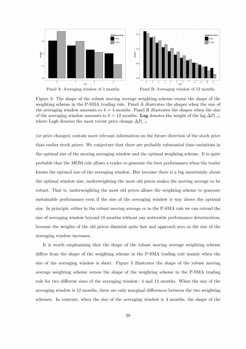
It is worth emphasizing that the shape of the robust moving average weighting scheme
differs from the shape of the weighting scheme in the P-SMA trading rule mainly when the
size of the averaging window is short. Figure 3 illustrates the shape of the robust moving
average weighting scheme versus the shape of the weighting scheme in the P-SMA trading
rule for two different sizes of the averaging window: 4 and 12 months. When the size of the
averaging window is 12 months, there are only marginal differences between the two weighting
schemes. In contrast, when the size of the averaging window is 4 months, the shape of the
28

robust weighting scheme is somewhere in between the shapes of the weighting schemes in the
MOM and P-SMA rules. That is, when the size of the averaging window is rather short, the
robust weighting scheme underweights older price changes to a lesser degree as compared with
that in the P-SMA rule.
To further demonstrate the advantages of the robust moving average, Table 3 reports
the rank of the robust moving average weighting scheme together with the ranks of the 3
active benchmark strategies for each 10-year period out of 30 overlapping periods. The active
benchmark strategies are the same as above: the MOM rule, the P-SMA rule, and the DCM.
We remind the reader that in our study there are totally 300 alternative weighting schemes.
As a result, the rank of a weighting scheme can be any integer number from 1 to 300. To
compute the ranks in this table, we use the size of the averaging window of 10 months. It
is worth noting that with this window size the best overall performance, among 4 competing
moving averages (see Table 2), is generated by the MOM rule; the second best by the P-SMA
rule; the robust moving average scores 3rd; the DCM has the worst performance. However,
the robust weighting scheme has the highest median rank and the second highest mean rank.
Even though the MOM rule generates the best performance over the total historical sample,
its median rank over all sub-periods, and especially the mean rank, is noticeable below those
of the robust moving average. Specifically, the mean rank of the MOM rule is higher than its
median rank. This tells us that the distribution of the performances of the MOM rule over sub-
periods is right-skewed. Apparently, the superior performance of the MOM rule tends to be
generated mainly over a few historical sub-periods. In contrast, for the robust moving average
the mean rank is virtually identical to the median rank. This tells us that the distribution of
the performances of the robust moving average over sub-periods is symmetrical. Finally, we
observe that out of 4 competing rules, the P-SMA rule most often outperforms the other rules
in sub-periods. Specifically, it is the best performing rule in 11 out of 30 sub-periods. Besides,
the P-SMA rule has the highest mean rank. Yet, the robust moving average has the highest
median rank over all sub-periods.
29
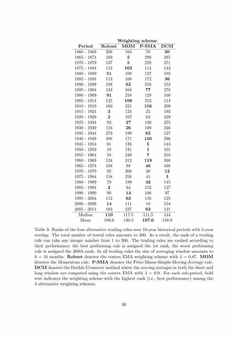
Weighting schemePeriod Robust MOM P-SMA DCM
1860 - 1869 206 164 76 301865 - 1874 169 5 290 2851870 - 1879 137 5 228 2711875 - 1884 112 102 114 1431880 - 1889 51 109 127 1031885 - 1894 113 108 172 361890 - 1899 198 62 216 1521895 - 1904 133 164 77 2781900 - 1909 91 218 129 1001905 - 1914 125 108 253 1141910 - 1919 160 221 156 2091915 - 1924 3 124 25 1931920 - 1929 2 107 63 2291925 - 1934 93 27 130 2551930 - 1939 116 26 109 2461935 - 1944 273 199 62 1271940 - 1949 286 171 150 2961945 - 1954 61 126 5 1431950 - 1959 19 181 1 1011955 - 1964 58 249 7 2101960 - 1969 124 212 119 2681965 - 1974 108 88 46 1681970 - 1979 92 206 38 121975 - 1984 158 256 41 31980 - 1989 79 189 42 1451985 - 1994 2 64 152 1271990 - 1999 90 14 186 971995 - 2004 112 63 116 1252000 - 2009 14 111 18 1542005 - 2014 103 237 63 121
Median 110 117.5 111.5 144Mean 109.6 130.5 107.0 158.0
Table 3: Ranks of the four alternative trading rules over 10-year historical periods with 5-yearoverlap. The total number of tested rules amounts to 300. As a result, the rank of a tradingrule can take any integer number from 1 to 300. The trading rules are ranked according totheir performance; the best performing rule is assigned the 1st rank, the worst performingrule is assigned the 300th rank. In all trading rules the size of averaging window amounts tok = 10 months. Robust denotes the convex EMA weighting scheme with λ = 0.87. MOMdenotes the Momentum rule. P-SMA denotes the Price-Minus-Simple-Moving-Average rule.DCM denotes the Double-Crossover method where the moving averages in both the short andlong window are computed using the convex EMA with λ = 0.9. For each sub-period, boldtext indicates the weighting scheme with the highest rank (i.e., best performance) among the4 alternative weighting schemes.
30

5 Conclusions
In this paper we presented the methodology to study the computation of trading indicators in
many market timing rules based on moving averages of prices and analyzed the commonalities
and differences between the rules. Our analysis revealed that the computation of every technical
trading indicator considered in this paper can equivalently be interpreted as the computation
of the weighted average of price changes over the averaging window. Despite a great variety
of trading indicators that are computed seemingly differently at the first sight, we found that
the only real difference between the diverse trading indicators lies in the weighting scheme
used to compute the moving average of price changes. The most popular trading indicators
employ either equal-weighting of price changes, overweighting the most recent price changes, or
a hump-shaped weighting scheme with underweighting both the most recent and most distant
price changes. The trading indicators basically vary only by the degree of over- and under-
weighting the most recent price changes.
As a practical application of our analysis, in this paper we also proposed and implemented
the novel method of selecting the moving average weighting scheme to use for the purpose of
timing the market. The criterion of selection was to choose the most robust moving average.
Robustness of a moving average was defined as its insensitivity to outliers and its ability to
generate sustainable performance under all possible market scenarios regardless of the size of
the averaging window. We performed the search over 300 different shapes of the weighting
scheme using 15 feasible sizes of the averaging window and many alternative segmentations of
the historical stock price data. Our results suggest that the convex exponential moving average
with the decay factor of 0.87 (for monthly data) represents the most robust weighting scheme.
We also found that the popular Price-Minus-Simple-Moving-Average trading rule belongs to
the top 5 most robust moving averages in our study.
References
Aronson, D. (2006). Evidence-Based Technical Analysis: Applying the Scientific Method and
Statistical Inference to Trading Signals. John Wiley & Sons, Ltd.
Berkowitz, J. and Kilian, L. (2000). “Recent Developments in Bootstrapping Time Series”,
Econometric Reviews, 19 (1), 1–48.
31

Brock, W., Lakonishok, J., and LeBaron, B. (1992). “Simple Technical Trading Rules and the
Stochastic Properties of Stock Returns”, Journal of Finance, 47 (5), 1731–1764.
Clare, A., Seaton, J., Smith, P. N., and Thomas, S. (2013). “Breaking Into the Blackbox:
Trend Following, Stop losses and the Frequency of Trading - The Case of the S&P500”,
Journal of Asset Management, 14 (3), 182–194.
Faber, M. T. (2007). “A Quantitative Approach to Tactical Asset Allocation”, Journal of
Wealth Management, 9 (4), 69–79.
Glabadanidis, P. (2015). “Market Timing With Moving Averages”, Forthcoming in Interna-
tional Review of Finance.
Gwilym, O., Clare, A., Seaton, J., and Thomas, S. (2010). “Price and Momentum as Robust
Tactical Approaches to Global Equity Investing”, Journal of Investing, 19 (3), 80–91.
Kilgallen, T. (2012). “Testing the Simple Moving Average across Commodities, Global Stock
Indices, and Currencies”, Journal of Wealth Management, 15 (1), 82–100.
Kirkpatrick, C. D. and Dahlquist, J. (2010). Technical Analysis: The Complete Resource for
Financial Market Technicians. FT Press; 2nd edition.
Moskowitz, T. J., Ooi, Y. H., and Pedersen, L. H. (2012). “Time Series Momentum”, Journal
of Financial Economics, 104 (2), 228–250.
Murphy, J. J. (1999). Technical Analysis of the Financial Markets: A Comprehensive Guide
to Trading Methods and Applications. New York Institute of Finance.
Okunev, J. and White, D. (2003). “Do Momentum-Based Strategies Still Work in Foreign
Currency Markets?”, Journal of Financial and Quantitative Analysis, 38 (2), 425–447.
Pagan, A. R. and Sossounov, K. A. (2003). “A Simple Framework for Analysing Bull and Bear
Markets”, Journal of Applied Econometrics, 18, 23–46.
Sharpe, W. F. (1994). “The Sharpe Ratio”, Journal of Portfolio Management, 21 (1), 49–58.
Sortino, F. A. and Price, L. N. (1994). “Performance Measurement in a Downside Risk Frame-
work”, Journal of Investing, 3 (3), 59 – 65.
Sullivan, R., Timmermann, A., and White, H. (1999). “Data-Snooping, Technical Trading
Rule Performance, and the Bootstrap”, Journal of Finance, 54 (5), 1647–1691.
Welch, I. and Goyal, A. (2008). “A Comprehensive Look at the Empirical Performance of
Equity Premium Prediction”, Review of Financial Studies, 21 (4), 1455–1508.
Zakamulin, V. (2014). “The Real-Life Performance of Market Timing with Moving Average
and Time-Series Momentum Rules”, Journal of Asset Management, 15 (4), 261–278.
32