anatomically constrained region deformation for the

www.elsevier.com/locate/ynimg
NeuroImage 34 (2007) 996–1019
Anatomically constrained region deformation for the automatedsegmentation of the hippocampus and the amygdala: Method andvalidation on controls and patients with Alzheimer’s disease

Marie Chupin,a,⁎ A. Romain Mukuna-Bantumbakulu,d Dominique Hasboun,b,c Eric Bardinet,b

Sylvain Baillet,b Serge Kinkingnéhun,d Louis Lemieux,a Bruno Dubois,d and Line Garnerob

aDepartment of Clinical and Experimental Epilepsy, Institute of Neurology, UCL, UKbCognitive Neuroscience and Brain Imaging Laboratory, CNRS UPR640, Paris, FrancecNeuroradiology Unit, Hôpital de la Salpêtrière, Paris, FrancedINSERM U610 unit, Paris, France

Received 30 June 2006; revised 25 October 2006; accepted 26 October 2006Available online 18 December 2006

We describe a new algorithm for the automated segmentation of thehippocampus (Hc) and the amygdala (Am) in clinical MagneticResonance Imaging (MRI) scans. Based on homotopically deformingregions, our iterative approach allows the simultaneous extraction ofboth structures, by means of dual competitive growth. One of the mostoriginal features of our approach is the deformation constraint basedon prior knowledge of anatomical features that are automaticallyretrieved from the MRI data. The only manual intervention consists ofthe definition of a bounding box and positioning of two seeds; totalexecution time for the two structures is between 5 and 7 min includinginitialisation. The method is evaluated on 16 young healthy subjectsand 8 patients with Alzheimer’s disease (AD) for whom the atrophyranged from limited to severe. Three aspects of the performances arecharacterised for validating the method: accuracy (automated vs.manual segmentations), reproducibility of the automated segmentationand reproducibility of the manual segmentation. For 16 young healthysubjects, accuracy is characterised by mean relative volume error/overlap/maximal boundary distance of 7%/84%/4.5 mm for Hc and12%/81%/3.9 mm for Am; for 8 Alzheimer’s disease patients, it is 9%/84%/6.5 mm for Hc and 15%/76%/4.5 mm for Am. We conclude thatthe performance of this new approach in data from healthy anddiseased subjects in terms of segmentation quality, reproducibility andtime efficiency compares favourably with that of previously publishedmanual and automated segmentation methods. The proposed approachprovides a new framework for further developments in quantitativeanalyses of the pathological hippocampus and amygdala in MRI scans.© 2006 Elsevier Inc. All rights reserved.

⁎ Corresponding author. MRI Unit, National Society for Epilepsy,Chesham Lane, Chalfont St Peter, SL9 0RJ BUCKS, UK. Fax: +44 1494875 666.

E-mail address: [email protected] (M. Chupin).Available online on ScienceDirect (www.sciencedirect.com).

1053-8119/$ - see front matter © 2006 Elsevier Inc. All rights reserved.doi:10.1016/j.neuroimage.2006.10.035

Introduction

The hippocampus (Hc) and the amygdala (Am) are medialtemporal lobe grey matter structures of primary importance infundamental cognitive processes and are involved in neurologicaland psychiatric diseases, including medial temporal lobe epilepsy(MTLE), Alzheimer’s disease (AD) and schizophrenia. Computa-tional studies of their anatomy are therefore crucial. Thesestructures form a small anatomical and functional complex withanatomically ill-defined internal and external boundaries, and aresubject to the partial volume effect, making their delineation inMagnetic Resonance Imaging (MRI) scans challenging.

Until recently, MRI volumetric studies of these structures havebeen based on careful manual segmentation (Hasboun et al.,1996; Pruessner et al., 2000) which is very time consuming(usually >1 h per structure) and suffers from considerable intra-and inter-rater variability (Bonilha et al., 2004; Free et al., 1995;Haller et al., 1997; Hogan et al., 2000; Pantel et al., 2000;Pruessner et al., 2000; Wieshmann et al., 1998). These factorslimit sensitivity to time-changes, disease-specific differences andinter-site comparisons. Reducing subjectivity through automationin the segmentation process is therefore highly desirable. Severalstrategies have been proposed to palliate the fuzziness of someboundaries.

Purely image-based methods generally rely on a manualinitialisation step. In Ashton et al. (1997), a region deformedelastically from a line of seeds according to a constraint, whereboth seeds and constraint were derived from manually segmentedcontours in three orthogonal slices. An artificial neural networksmethod was described by Pérez de Alejo et al. (2003), that reliedon unsupervised tissue-segmentation, followed by supervisedvolume identification trained on a manually segmented sagittalslice. A patch-based surface model was introduced by Ghanei et al.(1998, 2001), requiring manually defined starting contours.

mailto:[email protected]

http://dx.doi.org/10.1016/j.neuroimage.2006.10.035

http://www.sciencedirect.com

997M. Chupin et al. / NeuroImage 34 (2007) 996–1019

Automation was implemented for the initial step for two of thesemethods, with an atlas-based trained maximum likelihoodclassifier (Ashton et al., 2003) and landmarks derived from rulesrelated to relative position with respect to global brain landmarks(Siadat et al., 2004).

Statistical information derived from a learning base, as inatlas-based methods or deformable templates, has led to somefully automatic methods, with built-in constraints. Shape orappearance models have been used in several methods.Statistically learned deformation modes were combined withelastic deformations of Hc, constrained by intensity profiles inKelemen et al. (1999). A level-set method, constrained bystatistical priors on shape and neighbour-relations betweenanatomical structures (Yang et al., 2004) or intensity (Yang andDuncan, 2004), was proposed to simultaneously segment Hc andAm. In Duchesne et al. (2002), an atlas matching method wasguided by an active appearance model to segment Hc and Am,which was refined in Klemenčič et al. (2004), with anotherregistration algorithm to build the model for Hc only. Atlas-based, fully automated methods for the segmentation of severalstructures (amongst which Hc and Am), have used spatialinformation either implicitly, as in Fischl et al. (2002) from ananatomical probabilistic atlas, or explicitly, as in Zhou andRajapakse (2005) modelling intensity, spatial location and spatialrelationships in a fuzzy template.

Some methods have combined manually and statisticallyderived constraints. Shen et al. (2002) deformed a shape modelwith geometrical and statistical priors, introducing at least 50manually identified landmarks for segmenting Hc. A computa-tionally expensive high-dimensional brain mapping technique(Haller et al., 1997; Hogan et al., 2000) used a fluid registrationto segment Hc and required 28 landmarks to be identifiedmanually. We note that this algorithm is unique among those withuser interaction to have been subjected to a thorough evaluation ofreproducibility. A semi-automated post-processing step wasrequired in the hybrid method proposed in Pitiot et al. (2004);initialised by the registration of an hybrid MRI/structure atlas onthe target image, a group of templates was then deformedaccording to image, shape, distance and texture constraints in arule-controlled framework.

In this work, we present a new Markovian dual deformationmethod for the simultaneous segmentation of Hc and Am. The newmethod can be seen as an extension of the region-growingalgorithm proposed in Mangin et al. (1995) and Poupon et al.(1998) for the segmentation of the cortex and the major basalganglia. Furthermore, the method relies on a dual segmentationembedding a competition framework at the interface between Hcand Am, to ensure a correct behaviour in the unclear area betweenHc and Am.

In order to be more applicable to data from both young controlsand AD patients, it does not include statistical shape priors, whichcould bias the segmentation in atrophic cases. In fact, althoughthere have been demonstrations of the usefulness of statistical priorknowledge in segmentation algorithms applied to data from normalsubjects, such methods could be sub-optimal for the segmentationof diseased structures. Using a disease-specific atlas can lead tosegmentation performance improvements compared to generalatlases, as shown on data from AD or Mild Cognitive Impairment(MCI) patients (Carmichael et al., 2005); this result highlights theinfluence on the final segmentation of the type of subject used inthe atlas.

In a preliminary study on a restricted sample of controls andpatients (Chupin et al., 2006), we have observed that segmentationis rendered particularly difficult in cases with AD, due todegeneration of Hc which results in a large atrophy in patientseven in early stages of the disease, and to loss of image contrast.We propose introducing a constraint in the segmentation toovercome this problem while retaining execution speed withminimal user input (to increase reproducibility) and limiting biasin relation to atrophy. In the new method, prior anatomicalknowledge is explicitly considered, based on local systematicproperties around automatically retrieved landmarks at the borderof the structures. As opposed to statistical shape priors, anatomicalknowledge gives information which is less variable and lesssensitive to atrophy than shape and size (Bloch et al., 2005).These priors can use explicit knowledge, which is based on ananatomical description of the structures (topology, position,distances) and their relationships; this information is formalisedby simple rules on position, geometry and intensity (Barra andBoire, 2001). In order to be introduced as a constraint in asegmentation algorithm, anatomical knowledge can be modelledin fuzzy maps (Barra and Boire, 2001; Bloch et al., 2005) or in theenergy/force guiding the deformation process (Yang et al., 2004;Pitiot et al., 2004); in our method, the constraint is introduced inthe energy.

Finally, we wanted to address a difficulty with regard to theevaluation of the algorithm performance in the current literature.An extended evaluation of the method is thus proposed, based on arange of commonly used measures in order to facilitatecomparisons with published manual segmentation and automatedmethods.

Following the method’s detailed description, we will presentevidence of its validity and potential usefulness by comparingits outcome with manually segmented structures in MRI datafrom 16 representative healthy controls and 8 AD patients usingboth quantitative measures of agreement, with volume, regionoverlap and boundary distance measures, and thorough qualitativeevaluation.

Algorithm

Principle

The algorithm is an iterative competitive deformation processbetween two objects, OHc (for Hc) and OAm (for Am), in a back-ground BGHcAm. Regions deform following local topology-preserving transformations from an initial offset of seeds; as inMangin et al. (1995) and Poupon et al. (1998), it derives from aMarkovian model. We define a voxel front as the set of voxels atthe border of a deforming object. The growth proceeds by alternateiterative deformations of OHc and OAm through the re-classificationof voxels in the vicinity of the current voxel front. This is achievedby minimising a global energy functional, built following aBayesian framework in order to embody data attachment andcomposite priors. At each step, classification optimisation iscarried out using the Iterated Conditional Modes (ICM) algorithm(Besag, 1989), a robust deterministic method for classifiers basedon Markov random fields, widely used for image segmentation(Dubes et al., 1990). The segmentation process stops when stabilityis reached.

A competitive scheme is needed because the anatomical borderbetween Hc and Am – both grey matter structures – is very difficult

998 M. Chupin et al. / NeuroImage 34 (2007) 996–1019

to determine on MRI scans. This border consists of the alveus, athin white matter structure, sometimes combined with cerebro-spinal fluid (CSF) of the lateral ventricle. It is only partly visible onroutine MRI scans such as those used in this work, and is thereforean unreliable feature to block the segmentation of Hc alone. In ouralgorithm, the current OHc–OAm interface is automatically detectedat the beginning of each deformation step; competition isintroduced in the voxel re-classification process by consideringan interface-specific optimisation and dual regularisation (inter-face–non-interface) for Hc. Voxels detected as part of the interface(IHcAm) can be reclassified as either OHc or OAm; the fact that IHcAmincludes only voxels previously classified either as OHc or OAm,reduces the risk of including background voxels in one of theobjects.

Neuroanatomical landmarks, derived from the alveus, para-hippocampal gyrus, temporal horn of the lateral ventricle andisthmus are used to build priors to further constrain thesegmentation process. These structures are considered for thebasis of the anatomical priors, because they are commonly used byneuroanatomists during manual delineation, both at the interfaceand at the other borders of the two structures. During the iterativesegmentation process, 11 sets of landmarks are automaticallyretrieved at the border of OHc and OAm, corresponding to 11patterns. These follow rules defined locally in accordance with theMarkovian formalism. These rules are derived from formalempirical descriptions of patterns in brain anatomy, as seen onMRI scans, and described in Appendix A. These patterns can alsobe retrieved in atrophied structures. The segmentation is thenconstrained through regularisation: each landmark’s 26-neighbour-hood is divided into several likelihood zones, defined according toprior anatomical likelihood of their voxels to belong to Hc and Am.The computation of the energy is modified for these regions, to acton the deformations according to the anatomical likelihood, asdetailed in Appendix B.

Outline

The three main operational steps of the segmentation processare summarised here and presented in detail in the followingsection. The first step is manual, its influence being discussed inPerformance evaluation; the following steps are fully automatic.

Initialisation:

• Definition of a bounding box delimiting the region of interest(ROI) including Hc and Am;

• Placement of one seed in each structure (Hc and Am).
Alternate deformations:
• Resetting of landmarks to NULL set.

1 Brainvisa and The Anatomist are available at http://brainvisa.info/,under a license CeCILL licence version 2.

Homotopic deformation of Hc voxel front.

• Selection of ‘candidates’ to re-classification in the neighbour-hood of the voxels of the Hc front;

• Detection of interface voxels, landmarks and likelihood zones,ICM initialisation;

• Voxel re-classification (ICM energy optimisation): at eachiteration, for each voxel candidate, re-classification in theobject leading to the smaller local energy:▪ for non-interface voxels, re-classification is restricted toeither OHc or BGHcAm;

▪ for interface voxels, re-classification is restricted to eitherOHc or OAm.

Homotopic deformation of Am voxel front.• Selection of ‘candidates’ to re-classification in the neighbour-hood of the voxels of the Am front;

• Detection of interface voxels, landmarks and likelihood zones,ICM initialisation;

• Voxel re-classification (ICM energy optimisation):▪ for non-interface voxels, re-classification is restricted toeither OAm or BGHcAm;

▪ for interface voxels, re-classification is restricted to eitherOAm or OHc.

Convergence criterion and stopping.

Detailed algorithm description

InitialisationThe algorithm is implemented in the Brainvisa environment1

(Cointepas et al., 2001), the complete 3D visualisation beinghandled by The Anatomist software (Rivière et al., 2000). No pre-or post-processing is used.

A region of interest (ROI) is defined manually using a mouse-driven cursor in a dedicated graphical interface for each subject andfor each hemisphere. This contained Hc (about 2500 voxels) andAm (about 1250 voxels); the dimensions of the ROI are normallyapproximately 30×50×20 voxels. The purpose of this parallele-piped ROI is to significantly decrease memory load (Duchesne etal., 2002; Hogan et al., 2000). The ROI is defined by six boundingslices according to the following rules, illustrated in Fig. 1.

1) the medial limit corresponds to the sagittal slice immediatelymedial to the uncus and the lateral limit to the sagittal planecontaining the CSF ellipsoid of the temporal horn of the lateralventricle;

2) the anterior limit corresponds to the coronal slice after which agrey matter mass appears in the uncal white matter, just after theisthmus and the posterior limit to the slice after the grey mattermass under the crus fornicis disappears;

3) the inferior limit corresponds to the axial slice below which greymatter disappears inside the white matter of the parahippocam-pal gyrus and the superior limit to the slice above which greymatter is no longer visible along the fornix.

Two seeds are positioned in the extracted ROI, according to tworules: the seeds are located near the centre of Am and the head ofHc (HHc); they are both placed approximately at the same distancefrom the interface. The starting point of the automated segmenta-tion process consists of three objects; two 5×5×5-voxel cubescentred on the seeds (initial OHc and OAm), and all other voxelswithin the ROI classified as BGHcAm.

Alternate deformationsThe OHc and OAm growth follows an alternate iterative

procedure; the Hc front is considered first, followed by the Amfront. Each voxel front is scanned to identify voxel re-classificationcandidates and only voxels identified as simple points in the26-neighbour vicinity of the current voxel front are considered. Apoint is defined as simple for a given object if the topological

http://brainvisa.info/

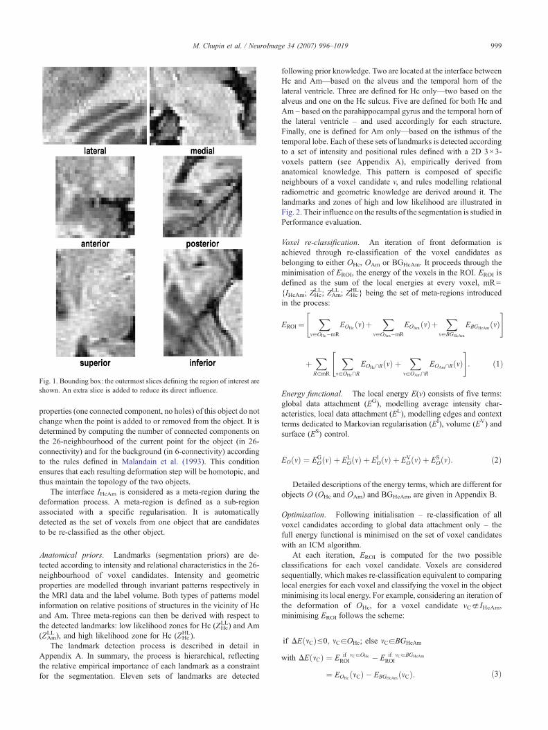
Fig. 1. Bounding box: the outermost slices defining the region of interest areshown. An extra slice is added to reduce its direct influence.


properties (one connected component, no holes) of this object do notchange when the point is added to or removed from the object. It isdetermined by computing the number of connected components onthe 26-neighbourhood of the current point for the object (in 26-connectivity) and for the background (in 6-connectivity) accordingto the rules defined in Malandain et al. (1993). This conditionensures that each resulting deformation step will be homotopic, andthus maintain the topology of the two objects.

The interface IHcAm is considered as a meta-region during thedeformation process. A meta-region is defined as a sub-regionassociated with a specific regularisation. It is automaticallydetected as the set of voxels from one object that are candidatesto be re-classified as the other object.

Anatomical priors. Landmarks (segmentation priors) are de-tected according to intensity and relational characteristics in the 26-neighbourhood of voxel candidates. Intensity and geometricproperties are modelled through invariant patterns respectively inthe MRI data and the label volume. Both types of patterns modelinformation on relative positions of structures in the vicinity of Hcand Am. Three meta-regions can then be derived with respect tothe detected landmarks: low likelihood zones for Hc (ZHc

LL) and Am(ZAm

LL ), and high likelihood zone for Hc (ZHcHL).

The landmark detection process is described in detail inAppendix A. In summary, the process is hierarchical, reflectingthe relative empirical importance of each landmark as a constraintfor the segmentation. Eleven sets of landmarks are detected

following prior knowledge. Two are located at the interface betweenHc and Am—based on the alveus and the temporal horn of thelateral ventricle. Three are defined for Hc only—two based on thealveus and one on the Hc sulcus. Five are defined for both Hc andAm – based on the parahippocampal gyrus and the temporal horn ofthe lateral ventricle – and used accordingly for each structure.Finally, one is defined for Am only—based on the isthmus of thetemporal lobe. Each of these sets of landmarks is detected accordingto a set of intensity and positional rules defined with a 2D 3×3-voxels pattern (see Appendix A), empirically derived fromanatomical knowledge. This pattern is composed of specificneighbours of a voxel candidate v, and rules modelling relationalradiometric and geometric knowledge are derived around it. Thelandmarks and zones of high and low likelihood are illustrated inFig. 2. Their influence on the results of the segmentation is studied inPerformance evaluation.

Voxel re-classification. An iteration of front deformation isachieved through re-classification of the voxel candidates asbelonging to either OHc, OAm or BGHcAm. It proceeds through theminimisation of EROI, the energy of the voxels in the ROI. EROI isdefined as the sum of the local energies at every voxel, mR={IHcAm; ZHc

LL; ZAmLL ; ZHc

HL} being the set of meta-regions introducedin the process:

EROI ¼X

maOHc�mR

EOHcðmÞþX

maOAm�mR

EOAm ðmÞþX

maBGHcAm

EBGHcAmðmÞ" #

þXRamR

XmaOHc\R

EOHc\RðmÞ þX

maOAm\REOAm\RðmÞ

" #: ð1Þ

Energy functional. The local energy E(v) consists of five terms:global data attachment (EG), modelling average intensity char-acteristics, local data attachment (EL), modelling edges and contextterms dedicated to Markovian regularisation (EI), volume (EV) andsurface (ES) control.

EOðmÞ ¼ EGOðmÞ þ EL

OðmÞ þ EIOðmÞ þ EV

OðmÞ þ ESOðmÞ: ð2Þ

Detailed descriptions of the energy terms, which are different forobjects O (OHc and OAm) and BGHcAm, are given in Appendix B.

Optimisation. Following initialisation – re-classification of allvoxel candidates according to global data attachment only – thefull energy functional is minimised on the set of voxel candidateswith an ICM algorithm.

At each iteration, EROI is computed for the two possibleclassifications for each voxel candidate. Voxels are consideredsequentially, which makes re-classification equivalent to comparinglocal energies for each voxel and classifying the voxel in the objectminimising its local energy. For example, considering an iteration ofthe deformation of OHc, for a voxel candidate vCg IHcAm,minimising EROI follows the scheme:

if DEðmCÞV0; mCaOHc; else mCaBGHcAm

with DEðmCÞ ¼ E if mCaOHcROI � E if mCaBGHcAm

ROI

¼ EOHcðmCÞ � EBGHcAmðmCÞ: ð3Þ

Fig. 2. Landmarks and associated likelihood zones. In each row, previously defined landmarks are kept and new ones are added. Left column shows correspondingsegmentation in the same slice. THVL=Temporal Horn of the Lateral Ventricle. Landmarks were illustrated in the orientation in which they are defined, except forthose derived from the parahippocampal gyrus, for which sagittal slices are more illustrative. In each case, the selected slice was chosen according to the number ofvoxels representing the illustrated landmark.



The ICM process stops when the deforming object is no longermodified, or when the number of changes is small enough duringthree consecutive ICM-iterations.

Convergence and stopping criterionThe overall deformation process ends when the number of

changes in both objects is smaller than 2% of their surface for threeiterations in a row.

Performance evaluation

We characterised performances by applying the algorithm indata from healthy subjects and AD patients, scanned in conditionsrepresentative of routine clinical investigations. Segmentationresults were evaluated in three ways: (1) accuracy: automatedresults were compared visually and quantitatively to manuallysegmented objects; (2) reproducibility: intra-observer and inter-observer reliability was considered in relation to inter-observerreliability of manually drawn results; (3) efficacy of the anatomicalpriors.

Material

MRI dataSixteen young healthy volunteers (S1–S16, age <35) and eight

patients with probable AD (P1–P8, mean age 74 (range: 66–81),mean MMSE (Mini Mental State Examination) 21 (6–28)) werescanned with a 1.5 Tesla Signa scanner (GE Medical Systems,Milwaukee, WI, USA). The acquisition parameters are sum-marised in Table 1. Image quality was characterised by thecontrast to noise ratio (CNR) and the contrast to noise and artefactratio (CNAR), which were defined as follows: contrast being thedifference between white and grey matter modes of the brainsignal intensity histogram; CNR=[contrast] / [intensity standarddeviation on a region of scan background without visibleartefacts]; CNAR [contrast] / [intensity standard deviation on thewhole background, including noise and visible artefacts (motion,wrap-around, pulsation)]. For S1–S16, CNAR=15±2 (13–19) andCNR=20±3 (16–25). For P1–P8, CNAR=11±3 (8–15) andCNR=15±4 (10–23). The slightly larger range of values forpatients could reflect the different sets of acquisition parameters(Li and Mirowitz, 2004).

Gold standard: manual segmentationThe manual segmentation protocol was established by a highly

trained neuroanatomist (Hasboun et al., 1996), and adapted to avoxel-based display environment. Images were manipulated with

Table 1Acquisition parameters for the images used in the evaluation process

TR TE TI Flip angle

S1–S8; S10–S16 14.3 ms a 6.3 ms a 600 ms 10°P1–P4; S9 10.3 ms 2.1 ms 600 ms 10°P5–P6 12.2 ms 5.3 ms 450 ms 15°P7–P8 9.2 ms 1.98 ms 600 ms 10°a TR=10.5 ms and TE=2.2 ms for S15.b Slice thickness of 1.5 mm for S7–S8.c 256×256 matrix for S15.d Coronal plane for P3.

the ROI-drawing module of The Anatomist software (Rivière et al.,2000). The boundaries of the two structures are described in detailin Appendix C and were principally determined on coronal sliceswith checks on simultaneous sagittal and axial views through alinked cursor.

The degree of atrophy in P1–P8 was obtained from manualsegmentations by expressing the difference between the volume ofeach structure and the mean volume of this structure for the younghealthy controls (YHC) (VHc

YHC=2.89 cm3, VAmYHC=1.40 cm3), in

units of standard deviation (σHcYHC=0.34 cm3, σAm

YHC=0.16 cm3).For Hc, the atrophy was [2.9±1.2 (0.9–4.4)] ·σHc

YHC and, for Am,the atrophy was [2.2±1.8 (−1.7–4.4)] ·σAm

YHC, which correspondedto limited to severe atrophy.

Based on automated segmentation results, the volume statisticsfor the young healthy controls were VHc

YHC=2.98 cm3 andVAmYHC=1.51 cm3, and the standard deviation σHc

YHC=0.36 cm3 andσAmYHC=0.21 cm3. For Hc, the atrophy was [3.1±1.5 (0.4–4.8)] ·

σHcYHC and, for Am, the atrophy was [2.5±1.1 (0.2–4.5)] ·σAm

YHC.

DesignThe simultaneous segmentation of Hc and Am took less than 1

min on a 1 GHz workstation with 512 MB RAM, developed inC++, in The Anatomist environment. The total segmentationprocess with ROI determination and seed positioning for bothstructures in both hemispheres (4 structures) took between 10 and15 min.

Four automated segmentations were performed: A1MC and A2

MC,initialised by operator MC on two different occasions, A1

RM,initialised by operator RM, and AnoAP

MC with the same ROI and seedsas A1

MC but without the anatomical priors. Two manual segmenta-tions were performed:M1

MC, by operator MC andM1DH, by operator

DH (S1–S6 only) or M1RM, by operator RM (P1–P8 only). The

results were qualitatively evaluated through 3D renderings andvisualisation of sagittal slices and quantitatively evaluated using 9indices defined in Appendix D: relative volume error (RV), spatialoverlap (K1, K2), False Positive rate (FP), False Negative rate (FN),Misclassified Interface Voxels (MIV), boundary distance (Dm,DM, D95).

For illustration purposes, we identified the best and worstresults according to the composite index CGQ which summarisesthe various aspects of the quantitative indices (accuracy andreproducibility), computed for comparisons A1

MC vs.M1MC and A2

MC

vs. A1MC (see Appendix D, Eq. (40)).

Local performance was evaluated by computing the relevantaccuracy indices, RV, K1, K2, FP, FN, DM and D95, for threesub-regions of Hc and two of Am, defined based on the partitionof the antero-posterior axis – from the first coronal slice which

Slice thickness Voxel size Orientation Matrix

1.3 mmb 0.9375 mm Axial 256×192 c

1.5 mm 0.9375 mm Axial d 256×1921.5 mm 0.976562 mm Coronal 256×1921.3 mm 0.9375 mm Coronal 256×256


contains the manually segmented structure to the last one – intothree equal segments for Hc, approximating head, body and tailand two segments (anterior third and the remaining two thirds)for Am.

The performance of landmark detection and landmark-derivedconstraints was also studied. The detection performance wascharacterised by the stability during deformations (number oflandmarks which were detected at some early iteration of thedeformations but no longer in the last iteration), the stability andaccuracy of the final set of landmarks (number of landmarks foreach type, correct and incorrect detection of low likelihood zonesoutside the manually segmented objects and high likelihoodzones inside the manually segmented objects). The effect of thepriors on performance was assessed by comparing the perfor-mance of the algorithm for A1

MC and AnoAPMC , and analysing the

improvement of CGQ.Note that all the parameters described in Appendix B were first

tuned on S1–S4, and refined on S5–S8 and P1–P4, on which onlyradiometric parameters could be tuned. No adjustment to thealgorithm was made for application to S9–S16 and only theanisotropy parameters were modified for P5–P8.

Fig. 3. 3D rendering for manual and automated segmentations

Evaluation on young healthy controls

Qualitative analysisManual and automated segmentations were inspected visually

for each subject and both hemispheres to assess their quality andlocalise any discrepancy. In general, automated segmentationtended to slightly over-estimate volume compared to manual one.Global shapes and some surface details were correctly recovered,while the main differences were in the tail and the head of Hc.

3D renderings of the best (S1 right hemisphere, S1R) andworst (S9 left hemisphere, S9L) results are displayed in Fig. 3 forM1

MC, A1MC, A2

MC, A1RM and AnoAP

MC . The shapes derived frommanual and automated segmentations matched well for bothobjects. Furthermore, 3D renderings for S1R indicate that surfacedetails extracted manually were also retrieved with the automatedsegmentation. Comparisons of the results with (A2

MC) and without(AnoAP

MC ) anatomical priors demonstrated their usefulness. Compar-isons of A1

MC, A2MC and A1

RM revealed a reproducible behaviour ofthe segmentation.

To localise false positives, false negatives and overlap, a fewsagittal slices are displayed for S1R and S9L (Fig. 4). For S1R,

for Am and Hc, for S1R and S9L. See text for details.

Fig. 4. Overlap between some pairs of the six segmentations for six sagittal slices (in the bounding box), for S1R and S9L for Seg vs. Ref. See text for details.Final likelihood zones for A1

MC are displayed in the “AP” rows with the same colour code as Fig. 2.


automated segmentations were almost identical. For S9L, the majorproblems were in the Am–Hc interface region. Differences bet-ween the automated segmentations with and without anatomicalpriors were clear for both.

Quantitative evaluation of segmentation qualityThe results are summarised in Table 2. Accuracy of the

automated method A1MC vs. M1

MC was close to manual reproduci-bility M1

MC vs. M1DH as revealed by the error on volume (RV=7%

(0–14) for Hc and 12% (1–27) for Am, compared to RV=7% (1–17) for Hc and 10% (1–24) for Am), the overlap (K1=84% (78–89)for Hc and 81% (69–88) for Am, compared to K1=90% (87–92)for Hc and 85% (81–92) for Am) and the maximal distance error(DM=4.5 mm (2.5–9) for Hc and 3.9 mm (2.8–6) for Am,

compared to DM=3.7 mm (2.3–6.2) for Hc and 3.1 mm (2.1–3.9)for Am). Automated intra (A2

MC vs. A1MC) and inter (A1

RM vs. A1MC)-

rater reproducibility was better than manual reproducibility(RV=2% (intra) and 4% (inter) for Hc and 9% (intra) and 8%(inter) for Am, K1=97% (intra) and 95% (inter) for Hc and 93%(intra) and 92% (inter) for Am and DM=2.5 mm (intra) and2.9 mm (inter) for Hc and 2.8 mm (intra and inter) for Am). Therelative segmentation error was greater for Am than for Hc. Notethat the error at the interface (MIV) is negligible compared to theglobal overlap error; the overlap error is roughly distributed aroundthe interface, as indicated by the average and maximal distanceerrors.

Segmentation quality index values for the subparts of Hc andAm are given in Table 3. RV, K1 and Dmax values revealed that thesegmentation was more accurate in the body and less accurate in

Table 2Quantitative indices for comparison between pairs of segmentations for S1–S16

Object Index A1MC vs. M1

MC A2MC vs. A1

MC A1RM vs. A1

MC AnoAPMC vs. M1

MC A1DH vs. M1

MC

Hc RV (%) 7±4 (0–14) 2±2 (0–6) 4±4 (0–15) 22±8 (4–37) 7±5 (1–17)K1 (%) 84±3 (78–89) 97±1 (94–99) 95±2 (91–99) 74±4 (66–85) 90±1 (87–92)K2 (%) 72±4 (64–79) 94±3 (88–99) 91±4 (83–98) 59±5 (49–74) 82±2 (76–84)FP (%) 15±3 (10–20) 3±2 (1–7) 5±4 (1–12) 29±4 (15–36) 6±2 (3–9)FN (%) 13±5 (4–21) 3±2 (0–8) 3±3 (0–15) 12±4 (6–24) 12±3 (8–19)MIV (%) 1.1±1 (0–3.7) 0.2±0.3 (0–1.1) 0.9±1.2 (0–4.2) 5.4±3.2 (0–12) 0.3±0.5 (0.0–1.9)Dm (mm) 0.5±0.1 (0.4–0.8) 0.1±0.1 (0–0.2) 0.2±0.1 (0–0.5) 1.1±0.3 (0.4–1.8) 0.3±0.1 (0.2–0.5)DM (mm) 4.5±1.5 (2.5–9) 2.5±0.8 (1.3–4.4) 2.9±0.9 (1.6–6) 7.4±2.6 (4–16) 3.7±1.2 (2.3–6.2)D95 (mm) 4±1.5 (1.9–8.5) 2.3±0.8 (1.3–4.2) 2.6±0.9 (1.6–5.5) 6.6±2.6 (3.4–15) 3.3±1.1 (1.9–5.4)

Am RV (%) 12±7 (1–27) 9±7 (0–30) 8±5 (0–19) 16±10 (2–41) 10±7 (1–24)K1 (%) 81±4 (69–88) 93±4 (78–99) 92±4 (80–99) 74±7 (53–88) 85±3 (81–92)K2 (%) 69±6 (53–78) 87±7 (64–98) 85±6 (67–97) 59±9 (36–79) 74±5 (68–85)FP (%) 19±6 (6–32) 4±4 (0–15) 7±5 (1–22) 27±7 (14–44) 14±6 (6–26)FN (%) 13±5 (5–25) 9±8 (0–29) 8±5 (0–21) 14±6 (6–31) 12±6 (4–21)MIV (%) 1.5±1 (0.3–3.8) 0.9±1.6 (0–6.6) 0.5±0.7 (0–2.6) 3.7±3.8 (0.1–17) 2.8±2.4 (0.4–7.1)Dm (mm) 0.7±0.2 (0.4–1.2) 0.3±0.2 (0–0.9) 0.3±0.1 (0–0.7) 1±0.4 (0.4–2.2) 0.5±0.1 (0.2–0.7)DM (mm) 3.9±0.9 (2.8–6) 2.8±1.2 (0.9–5.9) 2.8±0.7 (0.9–4.3) 5.4±1.5 (2.8–9.9) 3.1±0.5 (2.1–3.9)D95 (mm) 3.5±0.8 (2.5–5.2) 2.6±1.2 (0.9–5.6) 2.5±0.7 (0.9–4.3) 5±1.5 (2.5–8.8) 2.9±0.6 (1.9–3.9)

Values=average±standard deviation (minimum–maximum).


the tail for Hc (largest maximal distance error: 9 mm), whereas itwas less accurate in the anterior part of Am than in any othersubpart.

Finally, the usefulness of the anatomical priors can be seen bycomparing the first column of Table 2 to the fourth, which revealsan important increase of the overlap between automatic and manualsegmentations. The performance and influence of landmarkdetection are detailed in Fig. 5. The improvement brought by theanatomical priors was inversely correlated with the quality ofAnoAPMC , as shown in Fig. 5a ((Corr[CGQ(A1

MC)−CGQ(AnoPAMC ),CGQ

(AnoPAMC )]=−0.91). Fig. 5b shows that the landmarks tended to be

robustly detected during deformations. Note that the largestchanges in detected landmarks across iterations were for thetemporal horn of the lateral ventricle superior–anterior to Hc andthe parahippocampal gyrus medial to Am; important changes forthe parahippocampal gyrus medial and lateral to Hc occurredduring three times more iterations than for the other landmarks.The size of the final low and high likelihood zones appeared to berelated to the size of the underlying structures they were built from(Fig. 5c); the incorrect detections were generally negligible, exceptfor the parahippocampal gyrus medial to Hc.

Evaluation on Alzheimer’s patients

Qualitative analysisThe manual and automated segmentations were again inspected

visually for each subject and both hemispheres. In general, as for

Table 3Quantitative indices on subparts of both structures for the accuracy for S1–S161

Index Hc head Hc body H

RV (%) 13±8 (1–36) 12±7 (1–26)K1 (%) 83±5 (70–91) 85±3 (79–93)K2 (%) 71±7 (54–84) 75±5 (65–87)FP (%) 14±5 (3–23) 18±4 (9–26)FN (%) 15±9 (2–37) 8±4 (2–18)DM (mm) 4±1.4 (2.3–7.8) 2.8±0.6 (1.5–4.5) 3D95 (mm) 3.7±1.4 (1.6–7.4) 2.5±0.6 (1.5–4.1) 3


controls, global shapes and some surface details were correctlyrecovered, while the main differences were in the tail and the headof Hc. Comparison of automated segmentations with and withoutanatomical priors confirmed their usefulness in pathological data.

Three-dimensional renderings for the best (P4 right hemisphere,P4R) and worst (P5 right hemisphere, P5R) results for comparisonsbetween A1

MC, A2MC, A1

RM, AnoAPMC and M1

MC are displayed in Fig. 6.Comparisons of A1

MC, A2MC and A1

RM revealed good reproducibilityfor Hc. For the worst result, the tail of Hc was incomplete.

To visualise false positives, false negatives and overlap for andbetween the two structures, a few sagittal slices are displayed forP4R and P5R (Fig. 7). False positives and false negatives tended tobe homogeneously distributed, except in the anterior part of Amand the Am–Hc interface. As expected, inter-rater reproducibilitywas worse than intra-rater. For both subjects, problems could beobserved in the Am–Hc region.

Quantitative evaluationSegmentation results were evaluated with the nine quantitative

indices as summarised in Table 4. The accuracy of the automatedmethod was close to manual reproducibility, as revealed by theerror on volume (RV=9% (0–21) for Hc and 15% (1–42) for Am,compared to RV=8% (2–18) for Hc and 13% (3–34) for Am), theoverlap (K1=84% (78–88) for Hc and 76% (60–87) for Am,compared to K1=87% (83–89) for Hc and 80% (72–85) for Am)and the maximal distance error (DM=6.5 mm (4.1–14) for Hc and4.5 mm (3.1–5.7) for Am, compared to DM=3.7 mm (2–6.3) for

c tail Am anterior Am posterior

13±12 (0–46) 26±15 (6–62) 11±10 (1–38)81±6 (65–90) 78±6 (59–87) 85±4 (76–92)69±9 (48–82) 64±8 (42–77) 74±6 (61–85)15±7 (4–32) 27±11 (6–51) 10±4 (3–20)16±9 (4–42) 9±6 (2–24) 17±7 (7–34)

.3±1.4 (1.6–9) 3.8±1 (2.6–6) 3.2±0.7 (2.1–4.7)

.1±1.3 (1.6–8.5) 3.5±0.8 (2.1–5.4) 3±0.6 (1.9–4.6)

Fig. 5. Characterisation of landmark detection for S1–S16: (a) global improvement vs. global quality of AnoAPMC ; (b) total number of landmarks and number of

landmarks not detected in the final iteration (minimal, average and maximal value at each iteration of the deformation of A1MC); (c) size of the final likelihood

zones A1MC, with correct and incorrect classification compared to M 1

MC.


Hc and 4.3 mm (2.6–6.6) for Am). Automated intra- and inter-raterreproducibility was better than manual reproducibility (RV=6%(intra) and 7% (inter) for Hc and 12% (intra) and 21% (inter) forAm, K1=95% (intra) and 94% (inter) for Hc and 90% (intra) and82% (inter) for Am and DM=2.5 mm (intra) and 2.6 mm (inter)for Hc and 2.6 mm (intra) and 3.8 mm (inter) for Am). Meanvalues and standard deviations for volume indices remainedcomparable with those obtained for controls.

Segmentation quality index values for the subparts of Hc andAm are indicated in Table 5. RV, K1 and DM values revealed that

the segmentation was more accurate in the body and less in the tail,for Hc, with a largest maximal distance error of 14 mm. For Am,both parts showed similar accuracy.

Again, the values demonstrated the usefulness of the anatomicalpriors, and the improvement was inversely correlated with thequality of AnoAP

MC (Corr[CGQ(A1MC)−CGQ(AnoAP

MC ),CGQ(AnoAPMC )]=

−0.99), as shown in Fig. 8a. The robustness of landmark detectionduring the deformations was comparable to that obtained for younghealthy controls (Fig. 8b). Note that the largest changes in detectedlandmarks across iterations were for the temporal horn of the

Fig. 6. 3D rendering for manual and automated segmentations for Am and Hc, for P4R and P5R. See text for details.


lateral ventricle superior–anterior to Hc and inferior–posterior toAm; the changes for the other landmarks were very small. Finally,Fig. 8c shows a different repartition of the likelihood zonescompared to the young healthy controls, which reflects the effectof atrophy (the alveus at the interface was less recovered, becauseof large pools of CSF between Hc and Am, and the enlargement ofthe sulcus of Hc due to atrophy resulted in a larger detection oflandmarks for the sulcus of Hc).

Discussion

We have presented a new competitive region growing methodfor the automated segmentation of the hippocampus and theamygdala. We introduced anatomical priors derived from systema-tic geometrical knowledge modelled as patterns that could beidentified in both healthy subjects and patients. The method wasevaluated in healthy subjects and patients with AD, qualitativelyand using a set of quantitative indices characterising importantaspects of the segmentation: volume, shape and position.

A previous version of the method was described in Chupinet al. (in press, in French), with limited evaluation on data from 8young healthy controls, and its application on data from 4 patientswith AD (Chupin et al., 2006). In this present work, improvedanatomical priors and regularisation anisotropy were used and theirfull description is given for the first time; the method’s perfor-mance is evaluated in a larger number of healthy controls andpatients with extended evaluation design.

In the data from young healthy controls, the segmentationresults were visually satisfactory with regard to both global shapeand local details for both structures and their interface. The inter-rater reproducibility of the automated method surpassed that ofmanual segmentation, thereby justifying the proposed approach.Furthermore, the results demonstrated clearly that the anatomicalpriors improved the segmentation, the improvement being largerfor results which were initially worse. Mean values of thequantitative indices for the sixteen young healthy controls showeda good agreement with manual segmentation, with a K1 value of84% for Hc and 81% for Am, and RV values of 7% for Hc and12% for Am. The number of misclassified voxels could be directly

Fig. 7. Overlap between some pairs of the six segmentations for five sagittal slices (in the bounding box), for P4R and P5R for Seg vs. Ref. See text for details.Final likelihood zones for A1

MC are displayed in the “AP” rows with the same colour code as Fig. 2.


characterised through the computation of 1−K2. Nevertheless, thisindex is very sensitive, as shown by the translation study inAppendix D; in summary, we found a mean of 18% ofmisclassified voxels between manual segmentations, 28% betweenautomated and manual segmentations and 9% between automatedsegmentations, for Hc. The computation of the average distance(0.3 mm, 0.5 mm and 0.2 mm, respectively) shows that thesemisclassified voxels tend to be located close to the Hc–Aminterface. The segmentation results were less accurate in theanterior part of Am and the tail of Hc. A possible explanation is thefuzziness of the anterior border of Am and noise blurring thetransition from body to tail for Hc. This ill-definition of the anteriorborder of Am could also explain the higher sensitivity of thesegmentation to the definition of the anterior border of the ROI,compared to the other borders.

Visually, our results for AD patients generally matched themanual segmentation, with RV=9% and K1=84% for Hc. Indicesvalues for manual reproducibility were also less good than forcontrols, reflecting the difficulty of segmenting atrophied struc-tures. Atrophy characterisation showed very similar volumes formanual and automated segmentations for controls. The same trendwas also found for the atrophy of Hc in AD patients. For Am,automated volumes showed atrophy in all cases whereas manualvolumes showed a hypertrophy in some cases. This emphasised thedifficulty of the segmentation of Am on the available MRI scans.

Comparison with other methods

Regarding the manual gold standard, we noted that the protocolfor manual segmentation was not always described in published

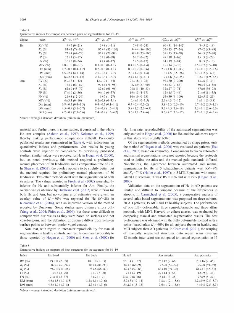
Table 4Quantitative indices for comparison between pairs of segmentations for P1–P8

Object Index A1MC vs. M1

MC A2MC vs. A1

MC A1RM vs. A1

MC AnoAPMC vs. M1

MC M1RM vs. M1

MC

Hc RV (%) 9±7 (0–21) 6±8 (1–31) 7±8 (0–24) 66±31 (14–142) 8±5 (2–18)K1 (%) 84±3 (78–88) 95±4 (82–100) 94±4 (86–100) 55±13 (27–74) 87±2 (83–89)K2 (%) 72±4 (64–79) 92±8 (70–99) 89±8 (75–100) 39±13 (15–58) 76±3 (72–80)FP (%) 12±4 (5–17) 5±7 (0–28) 6±7 (0–22) 47±18 (1–68) 15±3 (8–22)FN (%) 16±5 (8–24) 4±4 (0–17) 5±5 (0–17) 14±19 (2–84) 8±3 (5–13)MIV (%) 0.8±1.6 (0–6.3) 0.3±0.3 (0–1.1) 0.4±0.5 (0–1.4) 18±14 (0–36) 2.5±2.7 (0.5–10)Dm (mm) 0.7±0.2 (0.4–1.2) 0.2±0.3 (0–1.1) 0.2±0.2 (0–0.6) 2.9±1.8 (1.1–8.9) 0.4±0.1 (0.2–0.6)DM (mm) 6.5±2.4 (4.1–14) 2.5±1.6 (1–7.7) 2.6±1.2 (0–4.4) 13±4.5 (6.5–26) 3.7±1.2 (2–6.3)D95 (mm) 6±2.3 (3.9–13) 2.3±1.3 (1–6.7) 2.4±1.1 (0–4.1) 12±4.6 (5.2–25) 3.2±1 (1.9–5.5)

Am RV (%) 15±13 (1–42) 12±12 (1–44) 21±18 (1–78) 97±80 (0–200) 13±8 (3–34)K1 (%) 76±7 (60–87) 90±6 (76–98) 82±9 (57–90) 43±33 (0–83) 80±4 (72–85)K2 (%) 62±9 (43–77) 82±9 (61–96) 70±11 (40–83) 32±27 (0–71) 67±6 (56–73)FP (%) 17±10 (2–36) 9±10 (0–37) 19±13 (4–57) 12±15 (0–46) 21±6 (11–35)FN (%) 21±8 (12–39) 9±7 (1–27) 10±10 (0–33) 55±39 (4–100) 12±5 (5–23)MIV (%) 4±3.3 (0–10) 0.2±0.8 (0–3.1) 0.4±1 (0–3.5) 2.9±4.3 (0–12) 1±1.1 (0–3.8)Dm (mm) 0.8±0.3 (0.4–1.3) 0.4±0.3 (0.1–1.1) 0.7±0.4 (0.3–2) 3.8±3.3 (0.5–10) 0.7±0.2 (0.5–1.1)DM (mm) 4.5±0.9 (3.1–5.7) 2.6±0.9 (1.6–4.5) 3.8±1.2 (2.6–6.7) 9.3±4.5 (3.6–18) 4.3±1.1 (2.6–6.6)D95 (mm) 4.2±0.8 (2.5–5.6) 2.4±0.8 (1.5–4.2) 3.6±1.1 (2.4–6) 8.6±4.2 (3.3–17) 3.7±1.1 (2.4–6.4)



material and furthermore, in some studies, it consisted in the wholeHc–Am complex (Ashton et al., 1997; Kelemen et al., 1999)thereby making performance comparisons difficult. Previouslypublished results are summarised in Table 6, with indications onquantitative indices and performances. Our results in youngcontrols were superior or comparable to previously publishedstudies. Similar values were reported for Hc in Hogan et al. (2000),but, as noted previously, this method required a preliminarymanual placement of 28 landmarks and a computation time of 2 h.In Shen et al. (2002), the overlap appears to be slightly better, butthe method required the preliminary manual placement of 50landmarks. Two other methods dealt with the segmentation of bothstructures. The values reported in Fischl et al. (2002) were slightlyinferior for Hc and substantially inferior for Am. Finally, theoverlap values obtained by Duchesne et al. (2002) were inferior forboth Hc and Am, but no volume error estimates were given; anoverlap value of K1=80% was reported for Hc (N=28) inKlemenčič et al. (2004), with an improved version of the methodreported by Duchesne. Some studies gave distance errors only(Yang et al., 2004; Pitiot et al., 2004), but these were difficult tocompare with our results as they were based on surfaces and notvoxel-regions, and the definition of distance differs from betweensurface points to between border voxel centres.

Note that, with regard to inter-rater reproducibility for manualsegmentation in healthy controls, our results compare favourably tothose reported by Hogan et al. (2000) and Shen et al. (2002) for

Table 5Quantitative indices on subparts of both structures for the accuracy for P1–P8

Index Hc head Hc body

RV (%) 19±11 (2–39) 18±10 (1–33)K1 (%) 82±7 (67–92) 88±4 (81–93)K2 (%) 69±10 (51–86) 78±6 (68–87)FP (%) 10±4 (3–20) 19±7 (7–30)FN (%) 21±11 (5–37) 3±2 (1–9)DM (mm) 4.6±1.8 (1.9–8.5) 3.2±1.1 (1.9–6)D95 (mm) 4.3±1.7 (1.9–8) 2.9±1 (1.9–6)


Hc. Inter-rater reproducibility of the automated segmentation wasonly studied in Hogan et al. (2000) for Hc, and the values we reportin this study were slightly better.

Of the segmentation methods constrained by shape priors, onlythe method of Hogan et al. (2000) was evaluated on patients (Hsuet al., 2002) based on volumetry. Comparisons between automatedand manual segmentations were not reported because the protocolsused to define the atlas and the manual gold standards differed.Nonetheless, the agreement between automated and manualsegmentation for Hc in 5 schizophrenic patients was: RV=9%and K1=74% (Haller et al., 1997); in 5 MTLE patients with mono-lateral Hc sclerosis, it was: RV=11% and K1=75% (Hogan et al.,2000).

Validation data on the segmentation of Hc in AD patients arelimited and difficult to compare because of the differences inatrophy. In Carmichael et al. (2005), a comparative analysis ofseveral atlas-based segmentations was proposed on three cohorts:20 AD patients, 19 MCI and 15 healthy subjects. The performanceof one fully deformable, three semi-deformable and three affinemethods, with MNI, Harvard or cohort atlases, was evaluated bycomparing manual and automated segmentation results. The bestperformance was obtained with the fully deformable method with acohort-based atlas: K2~60% for all subjects (better in healthy andMCI subjects than AD patients). In Crum et al. (2001), the warpingof manually segmented structures onto repeat scans (average18 months inter-scan) was compared to manual segmentation in 15

Hc tail Am anterior Am posterior

22±14 (1–57) 26±17 (2–66) 20±16 (2–45)82±6 (68–91) 77±8 (56–86) 75±8 (59–89)69±8 (52–83) 63±10 (39–76) 61±11 (42–81)7±4 (3–19) 22±14 (1–54) 12±9 (3–34)

23±10 (8–46) 15±11 (3–38) 27±9 (8–39)5.2±3 (1.9–14) 3.8±1 (2.1–5.6) 4.2±0.9 (2.5–5.7)5±2.9 (1.8–13) 3.6±1 (2.1–5.6) 4±0.8 (2.5–5.3)

Fig. 8. Characterisation of landmark detection for P1–P8: (a) global improvement vs. global quality of AnoAPMC ; (b) total number of landmarks and number of

landmarks not detected in the final iteration (minimal, average and maximal value at each iteration of the deformation of A1MC); (c) size of the final likelihood

zones A1MC, with correct and incorrect classification compared to M 1

MC.


controls and 12 AD patients with the following results: RV=1%,K2=90%,2 and 5 subjects amongst the 27 had RV>5% andK2<85%.

Methodological and data issues

The use of data acquired in a purely clinical context, thereforepotentially sub-optimal compared to research data, is particularly

2 The definition of K2 utilised is unconventional.

interesting to test the algorithm’s robustness. The choice of thedifferent sequences used here was mainly dictated by previouslydefined protocols. We also wanted to test the algorithm on dataacquired according to more recent protocols, for which larger datasets were available. Some of the scans were discarded due to largemotion artefacts that rendered them un-interpretable.

Coronal orientation is usually preferred when studying Hcbecause the internal intricate details of Hc are better seen, andscans may even be acquired already reformatted perpendicular tothe long axis of Hc (Hasboun et al., 1996). Scans in our data setwere mainly acquired in the axial plane commonly used in non-Hc-

Table 6Summary comparison of our findings with previously published methods for automated segmentation of Hc and Am

A/M A/A M/M Samplesize

Cpu time Manualinteraction

Qualitativeevaluation

Manualprotocol

RV K1 Hm RV K1 Hm RV K1 Hm

Chupin H 7 84 0.5 4 95 0.2 7 90 0.3 32 <1 min Hc+Am Low Correct PreciseA 12 81 0.7 8 92 0.3 10 85 0.5

Hogan H 6 83 5 94 10 81 5 2 h Hc Medium Correct PreciseA

Schen H 6 88 3 86 20 High Smooth PreciseA

Fischl H 10 80 15 80 14 30 min UnclearA 15 65 25 75

Duchesne H 68 60 20 min Low Unclear PreciseA 63

Yang H 1.8 12 1 h per object Unclear UnclearA 1.6

Pitiot H 2.1 20 6 min, 4 objects High Unclear PreciseA

A/M: accuracy.A/A: inter-observer automated reproducibility.M/M: inter-observer manual reproducibility.Sample size: number of structures of each kind in the evaluation.Cpu time: computation time.Manual interaction: importance of the manual input in the method.Qualitative evaluation: aspect of the 3D renderings or overlap slices.Manual protocol: description of the protocol used in the manual segmentation to create the reference.


specific clinical routine, because it covers the whole brain withnearly isotropic voxels with good resolution and reduced scanningtime. The alveus at the interface between Hc and Am is less blurredby partial volume effect on axial scans, which makes the automateddiscrimination between Hc and Am more robust in 3D.

The parameters used in themethodwere first tuned on S1–S4 andthe radiometric parameters were refined on S5–S8 and P1–P8. Inorder to evaluate the influence of parameter tuning on the results andthe applicability of the method on ‘new’ (i.e. non tuning) data sets,accuracy results are given in Table 7 for S1–S8 and S9–S16 only andfor P1–P4 and P5–P8, showing that the values obtained for new datasets are similar to those obtained for the tuning data sets.

For controls, the worst result was obtained for S9, which wasacquired with different acquisition parameters, with 1.5 mm axialslices and had the lowest CNR in the control group. Note that thisacquisition was also used for P1–P4. In quantitative results, thesystematic difference between Hc and Am could be explainedpartly by the fact that Am, which is roughly half the size of Hc, hasblurred boundaries, and there was a significant pulsation artefactacross its anterior part in 10 subjects (Fig. 9).

Table 7Influence of the training set for parameter setting: statistics on S1–S8 (“tuning squantitative indices for the accuracy

Index S1–S8 S9–S16

Hc RV (%) 7±4 (1–13) 7±5K1 (%) 84±3 (80–89) 83±2MIV (%) 1.1±0.9 (0–3.2) 1.2±1.2DM (mm) 4.2±1.6 (2.5–9) 4.8±1.5

Am RV (%) 11±6 (2–21) 13±7K1 (%) 83±3 (77–88) 80±5MIV (%) 1.5±1.1 (0.4–3.7) 1.5±0.9DM (mm) 3.5±0.5 (2.8–4.6) 4.3±1


For AD patients, the two largest RV values for Hc for A1MC vs.

M1MC were obtained for P2, for which the mean ROI grey matter

intensity was consistently higher than the mean brain grey matterintensity, which was not the case for the other scans (except P7 lefthemisphere). This difference could be explained by the high levelof atrophy of the whole region and the under-representation of Hcgrey matter in the ROI histogram grey matter mode, resulting in anincorrect estimation of the average intensity of the hippocampus.Note that the largest RV values for Hc for A2

MC vs. A1MC and A1

RM

vs. A1MC were obtained for highly atrophic Hc (manual atrophy: 4.4

σHcYHC and 4.2 σHc

YHC, respectively). The worst result, according tothe combination of indices, was obtained for P5, for which theCNAR is the largest with a large amount of artefact. It can explainpropagation problems towards the tail of Hc and the highvariability of the segmentation for Am. Segmentation problemsat the interface region and distance errors larger than for controlscan be explained by the level of atrophy: when atrophy was severe,the grey matter in the head of Hc was reduced to a one-voxelribbon against the white matter of the alveus and the parahippo-campal gyrus (Fig. 10). Partial volume effect and noise made it

et”), S9–S16 (“test set”), P1–P4 (“tuning set”) and P5–P8 (“test set”) for

P1–P4 P5–P8

(0–14) 10±8 (0–21) 8±6 (0–15)(78–88) 83±2 (78–84) 85±3 (80–88)(0–3.7) 0±0.1 (0–0.3) 1.5±2 (0–6.3)(3–7.8) 6±1.2 (4.9–8.5) 7±3.2 (4.1–14)(1–27) 13±14 (1–42) 18±12 (1–35)(69–85) 77±5 (71–87) 76±9 (60–86)(0.3–3.8) 5.1±2.6 (0–8.9) 2.9±3.8 (0–10)(2.9–6) 4.6±0.9 (3.1–5.7) 4.4±0.9 (3.1–5.4)

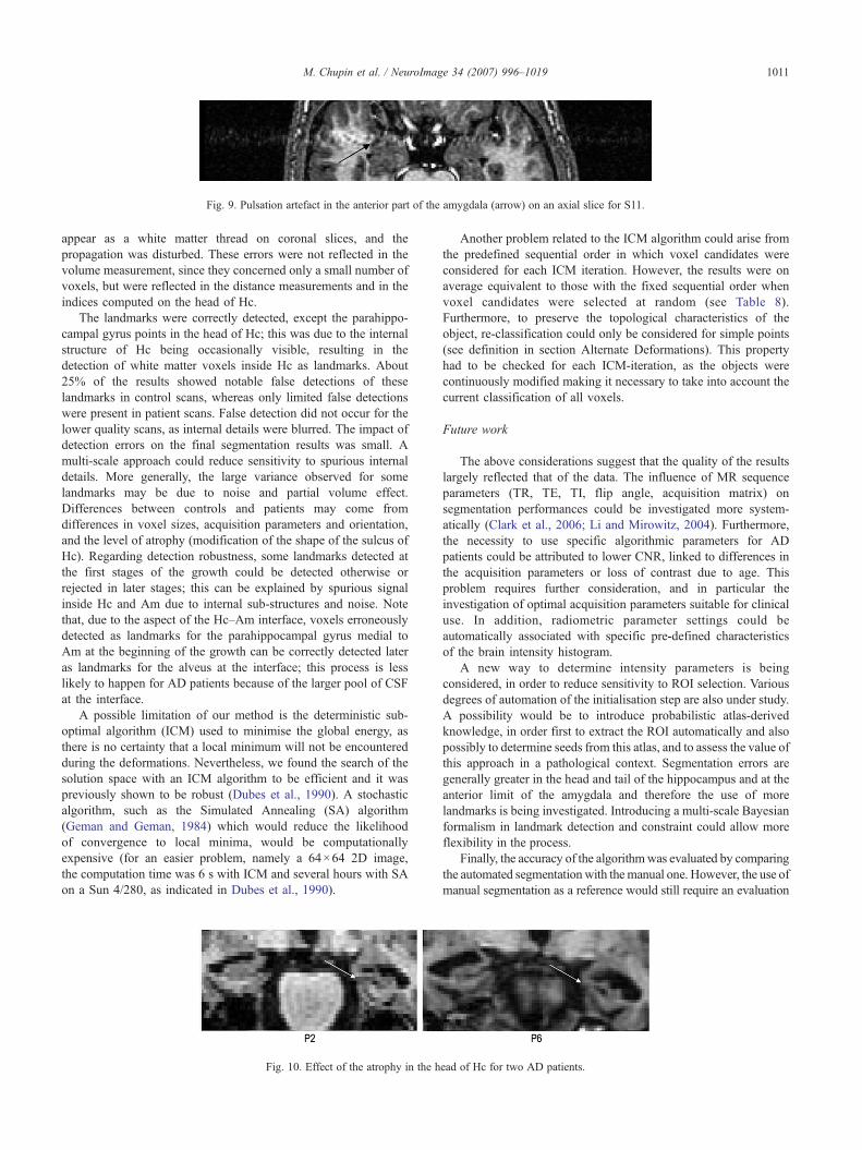
Fig. 9. Pulsation artefact in the anterior part of the amygdala (arrow) on an axial slice for S11.


appear as a white matter thread on coronal slices, and thepropagation was disturbed. These errors were not reflected in thevolume measurement, since they concerned only a small number ofvoxels, but were reflected in the distance measurements and in theindices computed on the head of Hc.

The landmarks were correctly detected, except the parahippo-campal gyrus points in the head of Hc; this was due to the internalstructure of Hc being occasionally visible, resulting in thedetection of white matter voxels inside Hc as landmarks. About25% of the results showed notable false detections of theselandmarks in control scans, whereas only limited false detectionswere present in patient scans. False detection did not occur for thelower quality scans, as internal details were blurred. The impact ofdetection errors on the final segmentation results was small. Amulti-scale approach could reduce sensitivity to spurious internaldetails. More generally, the large variance observed for somelandmarks may be due to noise and partial volume effect.Differences between controls and patients may come fromdifferences in voxel sizes, acquisition parameters and orientation,and the level of atrophy (modification of the shape of the sulcus ofHc). Regarding detection robustness, some landmarks detected atthe first stages of the growth could be detected otherwise orrejected in later stages; this can be explained by spurious signalinside Hc and Am due to internal sub-structures and noise. Notethat, due to the aspect of the Hc–Am interface, voxels erroneouslydetected as landmarks for the parahippocampal gyrus medial toAm at the beginning of the growth can be correctly detected lateras landmarks for the alveus at the interface; this process is lesslikely to happen for AD patients because of the larger pool of CSFat the interface.

A possible limitation of our method is the deterministic sub-optimal algorithm (ICM) used to minimise the global energy, asthere is no certainty that a local minimum will not be encounteredduring the deformations. Nevertheless, we found the search of thesolution space with an ICM algorithm to be efficient and it waspreviously shown to be robust (Dubes et al., 1990). A stochasticalgorithm, such as the Simulated Annealing (SA) algorithm(Geman and Geman, 1984) which would reduce the likelihoodof convergence to local minima, would be computationallyexpensive (for an easier problem, namely a 64×64 2D image,the computation time was 6 s with ICM and several hours with SAon a Sun 4/280, as indicated in Dubes et al., 1990).

Fig. 10. Effect of the atrophy in the h

Another problem related to the ICM algorithm could arise fromthe predefined sequential order in which voxel candidates wereconsidered for each ICM iteration. However, the results were onaverage equivalent to those with the fixed sequential order whenvoxel candidates were selected at random (see Table 8).Furthermore, to preserve the topological characteristics of theobject, re-classification could only be considered for simple points(see definition in section Alternate Deformations). This propertyhad to be checked for each ICM-iteration, as the objects werecontinuously modified making it necessary to take into account thecurrent classification of all voxels.

Future work

The above considerations suggest that the quality of the resultslargely reflected that of the data. The influence of MR sequenceparameters (TR, TE, TI, flip angle, acquisition matrix) onsegmentation performances could be investigated more system-atically (Clark et al., 2006; Li and Mirowitz, 2004). Furthermore,the necessity to use specific algorithmic parameters for ADpatients could be attributed to lower CNR, linked to differences inthe acquisition parameters or loss of contrast due to age. Thisproblem requires further consideration, and in particular theinvestigation of optimal acquisition parameters suitable for clinicaluse. In addition, radiometric parameter settings could beautomatically associated with specific pre-defined characteristicsof the brain intensity histogram.

A new way to determine intensity parameters is beingconsidered, in order to reduce sensitivity to ROI selection. Variousdegrees of automation of the initialisation step are also under study.A possibility would be to introduce probabilistic atlas-derivedknowledge, in order first to extract the ROI automatically and alsopossibly to determine seeds from this atlas, and to assess the value ofthis approach in a pathological context. Segmentation errors aregenerally greater in the head and tail of the hippocampus and at theanterior limit of the amygdala and therefore the use of morelandmarks is being investigated. Introducing a multi-scale Bayesianformalism in landmark detection and constraint could allow moreflexibility in the process.

Finally, the accuracy of the algorithmwas evaluated by comparingthe automated segmentation with themanual one. However, the use ofmanual segmentation as a reference would still require an evaluation

ead of Hc for two AD patients.

Table 8Statistics (on S1–S16) for quantitative indices for the accuracy with fixed order, average result, and best and worst indices values for random order (voxel frontand voxel candidates) on 20 trials

Index Fixed Average random Best random Worst random

Hc RV (%) 7±4 (0–14) 8±4 (1–15) 6±4 (0–13) 11±6 (2–30)K1 (%) 84±3 (78–89) 84±3 (78–89) 84±3 (80–89) 83±3 (75–88)MIV (%) 1.1±1 (0–3.7) 1.2±1.1 (0–3.7) 0.8±0.8 (0–3.5) 1.7±1.4 (0–4.9)DM (mm) 4.5±1.5 (2.5–9) 4.5±1.3 (2.4–8) 4±1 (2.1–6.5) 5.3±2.2 (3.1–14)

Am RV (%) 12±7 (1–27) 12±7 (1–28) 10±7 (0–25) 15±7 (2–30)K1 (%) 81±4 (69–88) 81±5 (69–88) 82±4 (72–89) 80±5 (65–87)MIV (%) 1.5±1 (0.3–3.8) 1.6±1 (0–3.8) 1.2±0.8 (0–3.6) 2.3±1.7 (0.4–6)DM (mm) 3.9±0.9 (2.8–6) 3.9±0.9 (2.8–6) 3.7±0.8 (2.8–6) 4.2±1 (2.8–6.4)



with histological comparison. This difficult problem is a limitation ofall MR-based segmentation of the hippocampus and amygdala andremains to be properly addressed.

Conclusion

We have presented a new automated hippocampus andamygdala MRI segmentation method. The competitive deformingregion algorithm was constrained by priors derived from anatomicalknowledge in the vicinity of landmarks that are automaticallydetected in healthy and diseased subjects. The algorithm’sperformance in terms of quality, reproducibility and computationtime compared favourably to that of manual segmentation and otherautomated methods.

Acknowledgments

The authors would like to thank Fabrice Poupon and DenisRivière for their help with the Anatomist software and ManikBhattacharjee for the transfer to Brainvisa. Marie Chupin wasfunded for this work by a grant from the France AlzheimerAssociation and a post-doctoral Marie Curie fellowship. The

Fig. 11. Hierarchical order when

authors would also like to thank Professor John Duncan and theNational Society for Epilepsy for their support. Finally, theauthors would like to thank Drs. Robert Powell and MahindaYogarajah for their helpful comments on English languageregarding the manuscript.

Appendix A. Landmark definitions and detection

The detection of the landmarks follows a hierarchical order,defined in Fig. 11. The detection rules are detailed in the followingparagraphs. Each is given in the form: if {set of conditions} then{set of actions}, in which all the conditions must be fulfilled. Thesix intensity thresholds used in the rules are derived from theautomatically estimated average intensities and tolerances for Hc,Am and the composite object HcAm. Their setting is given inAppendix B, section B.5.

A.1. Alveus at the interface between Hc and Am

The alveus is a thin (~1 mm) white matter structure. Its anteriorpart is between Hc and Am. To detect the location of the alveus at theinterface and use the complementary information that Am is superior

detecting the landmarks.


and anterior to Hc, we compare the 2D neighbourhood pattern of thevoxel in the sagittal slice with the following pattern:

P sagittal interfaceðmÞ ¼mAm mAmmAm m mHc

mHc mHc

24

35: ð4Þ

For the determination of the unlikely or likely zones for Hc andAm, the detection rules on the sagittal slice are:

if

card fmHcaOHcgz2 & card fmAmaOAmgz2

iðmÞz i alvcard fmAm ; with iðmAmÞV i alvg ¼ 3

8><>:

9>=>;;

then

mHcaZ LLAm & mHcaZ HL

Hc

mAmaZ LLHc

maZ HLHc

8><>:

9>=>;:

ð5Þ

The intensity threshold ialv is derived from the characteristicsfor Hc. Voxels vAm are not likely to belong to Am because of apossible presence of CSF between the alveus and Am.

A.2. Temporal horn of the lateral ventricle between Hc and Am

The temporal horn of the lateral ventricle (THLV) at theinterface appears as a dark CSF zone between Hc and Am; again,complementary information is deduced from the anatomicalposition of Am, superior and anterior to Hc. Psagittal_interface isused. When considering this interface, the corresponding detectionrules become:

ifcard fmHcaOHcgz2 & card fmAmaOAmgz2

iðmÞV iTHLV

� �;

then

mHcaZ LLAm

mAmaZ LLHc

maZ LLHc & maZ LL

Am

8><>:

9>=>;:

ð6Þ

When considering Hc, the detection rules are:

ifcard fmHcaOHcgz2 & card fmAmaOHcgV1

iðmÞV iTHLV

� �;

then

mHcaZ LLAm

mAmaZ LLHc

maZ LLHc & maZ LL

Am

8><>:

9>=>;:

ð7Þ

When considering Am, the detection rules are:

ifcard fmAmaOAmgz2 & card fmHcaOAmgV1

iðmÞV iTHLV

� �

then

mHcaZ LLAm

mAmaZ LLHc

mHcaZ LLHc & maZ LL

Am

8><>:

9>=>;:

ð8Þ

The intensity threshold iTHLV is derived from the characteristicsfor HcAm.

A.3. Alveus superior to Hc

The alveus also appears on the superior border of Hc. The 2Dpattern is defined on sagittal slices:

Psagittal superiorðmÞ ¼m� m�

mm* mþ mþ

24

35; ð9Þ

and the detection rules are:

if

cardfmþaOHc;m*aOHcg ¼ 3& cardfm�aOHcg ¼ 0

iðmÞzialviðm�ÞVialv & jiðm�Þ � iðmÞjzralv

8><>:

9>=>;;

then

m�aZ LLHc

mþaZ HLHc

maZ HLHc

8><>:

9>=>;:

ð10Þ

The intensity tolerance σalv is derived from the characteristicsfor Hc.

A.4. Alveus lateral to Hc

The alveus also appears on the lateral-superior border of Hc. The2D pattern is defined on coronal slices (displayed for the right side ofthe brain, in radiological convention; left side defined symmetrically):

Pcoronal lateral−superiorðmÞ ¼m� m�

m� m mþ

mþ mþ

24

35; ð11Þ


if

card fmþaOHcgz2 & card fm�aOHcg ¼ 0

iðmÞzialvjiðm�Þ � iðmÞjzralv

8><>:

9>=>;;

then

m�aZ LLHc

mþaZ HLHc

maZ HLHc

8><>:

9>=>;:

(12)

A.5. Sulcus of Hc

The sulcus of Hc has variable size and shape in normal anddiseased population. It appears on sagittal slices as a thin CSFspace in the head of Hc, roughly oriented in an anterio-posteriordirection. The 2D pattern is defined on sagittal slices:

Psagittal middleðmÞ ¼mP

mA m mP

mA

24

35; ð13Þ


if

iðmÞV i sulcuscardfmA; with mAgOHc & iðmAÞV isulcusgz1

cardfmP; with mPgOHc & iðmPÞV isulcusgz1

8><>:

9>=>;;

then

maZ LLHc

8mP; if fiðmPÞV isulcusg; then fmPaZ LLHc g

8mA; iffiðmAÞV i sulcusg; then fmAaZ LLHc g

8><>:

9>=>;:

ð14Þ


The intensity threshold isulcus is derived from the characteristicsfor HcAm.

A.6. Parahippocampal gyrus medial to Hc or Am

The parahippocampal gyrus white matter appears partly as awhite structure on the medial-inferior border of Hc and Am. The2D pattern is defined on coronal slices (displayed for the rightside of the brain, in radiological convention; left side definedsymmetrically):

Pcoronal medial−inferiorðmÞ ¼mþ mþ

mþ m m�

m� m� m�

24

35; ð15Þ

and the detection rules are, for Hc:

if

card fmþaOHcg ¼ 3 & card fm�aOHcg ¼ 0

iðmÞz iGPHcard fiðm�Þz iGPHgz1

8><>:

9>=>;;

then

m�aZ LLHc

m�aZ LLAm

maZ LLHc

8><>:

9>=>;:

ð16Þ

and for Am:

if

card fmþaOAmg ¼ 3 & card fm�aOAmg ¼ 0


8><>:

9>=>;;

thenm�aZ LL

Am

m�aZ LLAm

( ):

ð17Þ

The intensity threshold iGPH is derived from the characteristicsfor HcAm.

A.7. Parahippocampal gyrus lateral to Hc or Am

The parahippocampal gyrus white matter also appears as awhite structure on the lateral-inferior border of Hc and Am. The2D pattern is defined on coronal slices (displayed for the rightside of the brain, in radiological convention; left side definedsymmetrically):

Pcoronal lateral−inferiorðmÞ ¼mþ mþ

m� m mþ

m� m� m�

24

35; ð18Þ

and the detection rules are, for Hc:

if

card fmþaOHcg ¼ 3 & card fm�aOHcg ¼ 0

iðmÞz iGPHcard fiðm�ÞziðmGPHgz1

8><>:

9>=>;;

then

m�aZ LLHc

m�aZ LLAm

maZ LLHc

8><>:

9>=>;:

ð19Þ

and for Am:

if

card fmþaOAmg ¼ 3 & card fm�aOAmg ¼ 0


8><>:

9>=>;;

thenm�aZ LL

Am

m�aZ LLAm

( ):

ð20Þ

A.8. Temporal lobe isthmus for Am

The isthmus is a white matter bridge on the lateral-superiorborder of Am. Pcoronal_lateral-superior is used. The detection rules are:

ifcardfmþaOHcg ¼ 3 & cardfm�aOHcg ¼ 0

iðmÞz i isthmus

� �;

thenm�aZ LL

Am

maZ LLAm

( ):

ð21Þ

The intensity threshold i isthmus is derived from the character-istics for HcAm.

A.9. Low likelihood zones propagation

ZHcLL and ZAm

LL are grown amongst candidate voxels followingrules that were used to create them, except for the sulcus of Hc,for which no propagation was considered. ZHc

HL could not bepropagated in the same way, due to the convex shape of Hc. Thepropagation followed the following hierarchical order: alveus atthe interface, alveus superior to Hc, the four parahippocampalgyrus landmarks together, alveus lateral to Hc (when consideringthe Hc front) or isthmus (when considering the Am front), andTHLV.

Appendix B. Energy functional

B.1. Global data attachment term

The term for the objects O, EOG (v), is based on global

characteristics of the structure’s intensity distribution. The intensityvalue at voxel v, i(v), is compared with ĩO, the average intensityvalue of O, with σO

G a standard deviation characterising theintensity range around ĩO. The energy term for BGHcAm is definedto exclude the intensities of both Hc and Am, defined as a singleobject OHcAm; intensity and tolerance for OHcAm are the average ofthose for OHc and OAm. Therefore:

EGO mð Þ ¼ iðmÞ � iO

rGO

� �2

EGBGHcAm

mð Þ ¼ 1

EGO HcAm

þ e

;

8>>><>>>:

ð22Þ

with e << 1r GO

� �2introduced to ensure numerical stability when

i(v)= ĩO.Fig. 12 illustrates the effect of data attachment terms on a

schematic drawing. The desired segmentation is delineated on the

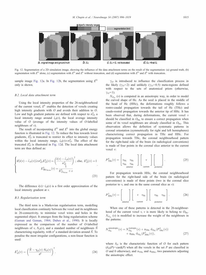
Fig. 12. Segmentation of a 2D simulation image, showing the influence of the data attachment terms on the result of the segmentation: (a) ground truth, (b)segmentation with EG alone, (c) segmentation with EG and EL without truncation, and (d) segmentation with EG and EL with truncation.


sample image Fig. 12a. In Fig. 12b, the segmentation using EG

only is shown.

B.2. Local data attachment term

Using the local intensity properties of the 26-neighbourhoodof the current voxel, EL enables the detection of voxels creatinghigh intensity gradients with O and avoids their addition to O.Low and high gradient patterns are defined with respect to σO

L, alocal intensity range around îO(v), the local average intensityvalue of O (average of the intensity values of O-labelledneighbours of v).

The result of incorporating EG and EL into the global energyfunction is illustrated in Fig. 12. To reduce the bias towards lowergradients, EO

L is truncated to restrict its effect to intensity valueswithin the local intensity range, îO(v)±σO

L. The effect of thetruncated EO

L is illustrated in Fig. 12d. The local data attachmentterm are thus defined as:

if ji mð Þ � iˆO mð ÞjzrLO;E

LO mð Þ ¼ iðmÞ � iˆOðmÞ

rLO

� �2

; else; E LO mð Þ ¼1

E LBGHcAm

mð Þ ¼ 1

E LO HcAm

þ e

:

8>>><>>>:

ð23Þ

The difference i(v)− îO(v) is a first order approximation of thelocal intensity gradient at v.

B.3. Regularisation term

The third term is a Markovian regularisation term, modellinglocal classification continuity between the voxel and its neighboursin 26-connectivity, to minimise voxel wires and holes in thesegmented object. It emerges from the Ising regularisation scheme(Geman and Geman, 1984; Dubes et al., 1990). It is locallyexpressed as the comparison of the number of O-labelledneighbours of v, NO(v), and a standard number of neighbours Ñcharacterising regularity, with σI a standard deviation around Ñ. Topenalise the most irregular configurations, a non-linear function isused:

E IO mð Þ ¼ N � gOðmÞdNOðmÞ

rI

� �5

: ð24Þ

γO is introduced to influence the classification process inthe likely (γO=2) and unlikely (γO=0.5) meta-regions definedwith respect to the sets of anatomical priors (otherwise,γO=1).

NOHc(v) is computed in an anisotropic way, in order to model

the curved shape of Hc. As the seed is placed in the middle ofthe head of Hc (HHc), the deformations roughly follows arostro-caudal propagation towards the tail of Hc (THc) andcaudo-rostral propagation towards the anterior tip of HHc. It hasbeen observed that, during deformations, the current voxel vshould be classified in OHc to ensure a correct propagation whensome of its voxel neighbours are already classified in OHc. Thisobservation allows the definition of systematic patterns incoronal orientation (symmetrically for right and left hemispheres)characterising correct propagation in THc and HHc. Forpropagation towards THc, the coronal neighbourhood patternfor the right-hand side of the brain (in radiological conventions)is made of four points in the coronal slice anterior to the currentvoxel v:

P 4THcðmÞ ¼ mHc mHc

mHc mHc

24

35

anterior

m

24

35

current

24

35

posterior

: ð25Þ

For propagation towards HHc, the coronal neighbourhoodpattern for the right-hand side of the brain (in radiologicalconventions) is made of three points (two in the coronal sliceposterior to v, and one in the same coronal slice as v):

P 3HHcðmÞ ¼

24

35

anterior

m mHc

24

35

current

mHc mHc

24

35

posterior

: ð26Þ

When one of these patterns is detected in the 26-neighbour-hood of the current voxel v, v is more likely to belong to OHc.NOHc

(v) is modified to increase the weight of the neighbours inthe patterns:

N anisotropicOHc

ðmÞ ¼ N isotropicOHc

ðmÞ þ aTHcddOHcðP 4THcðmÞÞ

þ aHHcddOHcðP 3HHcðmÞÞ; ð27Þ

where δO is the characteristic function of O for each pattern(δO(P)=card(P) when all the voxels in the set P are classified inO and 0 otherwise), and αTHc and αHHc, two parameters adjustingthe anisotropic effect.


B.4. Surface and volume terms

These two terms are introduced to prevent O from growingwhen the volume (number of voxels in O, VO(v)) and surface(number of surface voxels of O, SO(v)) reach unrealisticallylarge values above given thresholds (VO* and SO*). These termsshould not influence the deformation process while volume andsurface are under their associated thresholds. Since thesegeometric characteristics are meaningless for BGHcAm, a pressureterm is used instead (θ positive value) to favour growth; thispressure term influences re-classification of voxel candidatesotherwise undecided and prevents unsatisfactory behaviourswhen the objects O stop growing because of a slight localminimum.

if VO mð Þ < V*O ; EVO mð Þ ¼ 0; else; EV

O mð Þ ¼ VOðmÞ � V*OrVO

!2

EVBGHcAm

ðmÞ ¼ h

;

8><>:

ð28Þand

if SO mð Þ < S*O ;ESO mð Þ ¼ 0; else; E S

O mð Þ ¼ SOðmÞ � S*OrSO

!2

ESBGHcAm

ðmÞ ¼ h

;

8><>:

ð29Þ

with σOV (or σO

S ) a standard deviation characterising volume (orsurface) range.

B.5. Parameter setting

The value of the 13 parameters used in the energy functionalwas either calculated automatically or fixed in the program asdescribed in Table 9.

B.5.1. Radiometric parametersMean intensity values, iO, and intensity ranges, σO

G and σOL, are

related to the scan properties and therefore computed from the datausing sequence dependant factors. They were derived from themean intensity and standard deviation of grey matter on the ROI(GM and σGM); these were automatically retrieved from a histogramanalysis on the ROI. For Hc, the mean intensity was empirically setat iHc=0.95.iGM. Our observation showed that Hc was to be

Table 9Settings of the parameters used in the energy functional

Parameter σG i σL ε σL αTHc

Setting PSC/PSS PSC PSC/PSS PSF PSF PSF/PSHc – – – 0.001 2 1, 2 orAm – – – 0.001 2

PSS=sequence dependant.PSC=computed in the program.PSF=fixed in the program.PSL=derived from the literature.

considered slightly brighter than Am to ensure correct competition.To force this difference between the two average intensity values,ĩAm=0.9.iGM.

For Hc, the global intensity range was empirically set atσHcG =2σGM for controls’ scans and σHc

G =2.5σGM for patients’scans. For Am, it was empirically set at σAm

G =1.4σGM. The localintensity range, σL, was set to σO

L =0.4σOG for the controls’ scans

and σOL =0.5σO

G for the patients’ scans; this ratio was inferred fromthe fact that the local intensity characterisation had to be moreacute than the global one. The difference between sequence-dependant factors came from contrast decrease in patients’ scans,which were of lesser quality.

Intensity thresholds for the detection of landmarks were empiri-cally derived from iHc and iAm: ialv= iHc+0.4σHc

G , σalv=0.4σHcG ,

iTHLV= iHcAm−1.5σHcAmG , isulcus = iHcAm−σHcAm

G , iGPH= iHcAm+0.7σHcAm

G and iisthmus= iHcAm+σHcAmG .

B.5.2. Geometric parametersIsing parameters were derived from geometrical considerations

on the 26-neighbourhood (Ñ and σI). Ñ was set as half theneighbourhood size. The standard deviation σI was set to 2 toavoid irregularities such as wires (high risk if v was included buthad less than 10 neighbours) or holes (high risk if v was excludedbut had more than 16 neighbours). The two parameters adjustinganisotropic regularisation for Hc appeared to be sensitive tonoise, and thus to be sequence-dependent and were tunedaccordingly. Note that for P7 the anisotropy parameters wereadapted on the left-hand side to compensate for low contrast andhigh noise.

Surface and volume terms were necessary to prevent the objectsfrom growing further than reasonable sizes. Thresholds, VO* andSO*, and ranges, σO

V and σOS , were thus set to control the relative

influence of EV and ES in the energy functional. VO* and SO* valueswere derived from average values obtained from manual segmen-tations of a sample of young controls; we checked that volumeaverages corresponded to the values given in the literature, withequivalent manual protocols (Pruessner et al., 2000), but there wasno data available for the surface values. Ranges were set largeenough to allow variations larger than the typical inter-individualvariability. Thus, the constraint derived from the thresholds wouldinfluence the deformation process when VO≥VO*+σO

V and SO≥SO*+σOS , high above average values. These terms were not modified for

patient data, so that the algorithm could be used without knowingthe diagnostic. The enlargement of the Hc sulcus was likely tomodify the ratio volume/surface, but this did not influence thesegmentation performance. The parameter θ was set to a smallvalue; the pressure force was efficient only in cases for which theclassification was unresolved by the other energy terms.

αHHc Ñ V* σV S* σS θ

S PSF/PSS PSF PSL PSL PSL PSL PSF3 0 or 2 13 2750 700 1950 500 0.1

13 1250 600 900 450 0.1


Appendix C. Manual segmentation protocol

The cornu amonis, the dentate gyrus, the alveus, the fimbria, and the part of the subiculum directly inferior to the cornu amoniswere includedin Hc. The medial limit was geometrically derived from the fimbria. If this structure was not visible on a slice, we used the junction between thelateral curved part and the medial flat part of the subiculum, as it appeared on coronal slices. The most anterior and posterior coronal slices weregiven by the alveus and the disappearance of grey matter under the crus fornicis, respectively.

As for Am, the superior limit was determined following the endorhinal sulcus. The medial limit, when not entirely defined by the whitematter of the uncal and entorhinal gyri, was drawn by prolonging it. The lateral limit was given by the white matter of the isthmus. Theposterior limit was defined by the alveus, and the most anterior coronal slice was found by scrolling backward until a grey matter massappeared in the white matter of the uncal gyrus, with reference to sagittal slices.

Appendix D. Segmentation quality indices

They compare the segmentation result Seg with the gold standard Ref. Nine indices were used to quantify the accuracy of the method andfacilitate comparison with published values (Gerig et al., 2001).

RV is the relative error on volume; it compares volumes for segmented object OSeg and reference object ORef, relatively to the average ofboth:

RV O Seg;ORef� ¼ 2

jVO Seg � VO Ref jVO Seg þ VO Ref

: ð30Þ

The optimal value for this index is 0%. Five measures are then used to quantify the number of properly classified voxels. The first twocharacterise overlap between OSeg and ORef; they correspond to two ways in which the similarity index can be computed. K1 is written:

K1 OSeg;ORef� ¼ 2

VO Seg\O Ref

VO Seg þ VO Seg: ð31Þ

This index, largely used in the literature, characterises the number of properly classified voxels, without taking into account the number ofill-classified voxels. It is thus less discriminative than K2:

K2 OSeg;ORef� ¼ VO Seg\O Ref

VO Seg[O Ref: ð32Þ

The optimal value for both indices is 100%. The numbers of false positives, FP, and false negatives, FN, are computed here relatively tothe number of voxels labelled as OSeg or ORef:

FP OSeg;ORef� ¼ VO Seg � VO Seg[O Ref

VO Seg\O Ref; ð33Þ

FN O Seg;ORef� ¼ VO Ref � VO Seg\O Ref

VO Seg[O Refð34Þ

Both are optimal when equal to 0%. They can be related to the overlap index through:

FPðOSeg;ORef Þ þ FNðOSeg;ORef Þ ¼ 1� K2ðOSeg;ORef Þ ð35ÞFinally, we introduce a new index, called Misclassified Interface Voxels (MIV), which quantifies the number of voxels labelled as O1 in

the segmentation and as O2 in the reference:

MIV OSeg1 ;ORef

1 ;ORef2

� �¼ 2

VO Seg1 \O Ref

2

VO Seg1

þ VO Ref1

: ð36Þ

Its optimal value is 0%.In order to estimate the sensitivity of these indices, one can compute them for simple deformations of a manual segmentation of Hc and

Am. Let ORef+T be ORef translated by a vector T. If T=(1,1,1), the values of the overlap ratios were: for Hc, K1(ORef +T, ORef)=64% and

K2(ORef +T, ORef)=47%; for Am, K1(O

Ref +T, ORef)=71% and K2(ORef +T, ORef)=55%; for the misclassified interface voxels, for Hc, MIV

(ORef−T, ORef)=7.7% and for Am, MIV(ORef +T, ORef)=16.4%. Let ORef.M be ORef morphologically eroded (M=E) or dilated (M=D)with a 1-voxel element. The values of the error on volume were: for Hc, RV(ORef.E, ORef)=36% and RV(ORef.D, ORef)=29%; for Am,RV(ORef.E, ORef)=44% and RV(ORef.D, ORef)=34%.

The local behaviour on the boundary can be characterised by its surface voxels (defined as the voxels of O with at least one 26-neighbouroutside of O). The distance between the centre of the surface voxels of OSeg and those of ORef is considered in three ways. First, the averagesymmetric distance on the whole boundary, Dm, is computed:

DmðOSeg;ORef Þ ¼ max½hðOSeg;ORef Þ;hðORef ;OSegÞ�; ð37Þ


with

h A;Bð Þ ¼ 1NA

XaaA

d a;Bð Þ:

Second, the maximum of the symmetric distance (Hausdorff distance), DM, is considered:

DMðOSeg;ORef Þ ¼ max½HðO Seg;ORef Þ;HðORef ;OSegÞ�; ð38Þwith

HðA;BÞ ¼ maxaaA

½dða;BÞ�; ð39Þ

with d the Euclidian distance.Finally, the last index is used to discard sporadic errors, by considering the distance which explains the 95 percentile of DM, and it was

called D95. All distances are expressed in millimetres.A composite index, GCQ, is defined which synthesises the various information brought by the above indices. GCQ is a combination of

global quality indexes, GQ(O,Seg), built from four quantitative indices, for Hc and Am:

GQðO;SegÞ ¼ 100:ðRVðO Seg;ORef Þ þ 1� K1ðOSeg;ORef Þ þ 2:MIVðOSeg;ORef ÞÞ þ 5:DMðO Seg;ORef ÞCGQðSegÞ ¼ 3:GQðOHc;SegÞ þ GQðOAm;SegÞ :

�ð40Þ

The optimal value for this global index is 0.

References

Ashton, E.A., Parker, K.J., Berg, M.J., Chen, C.W., 1997. A novelvolumetric feature extraction technique with applications to MR images.IEEE Trans. Med. Imag. 16 (4), 365–371.

Ashton, E.A., Riek, J., Molinelli, L., Berg, M., Parker, K., 2003. A methodfor fully automated measurement of neurological structures in MRI.SPIE Medical Imaging-2003, vol. 5032, pp. 1125–1134.

Barra, V., Boire, J.-Y., 2001. Automatic segmentation of subcortical brainstructures in MR images using information fusion. IEEE Trans. Med.Imag. 20 (7), 549–568.

Besag, J., 1989. Towards bayesian image analysis. J. Appl. Stat. 16 (3),395–407.

Bloch, I., Colliot, O., Camara, O., Géraud, T., 2005. Fusion of spatialrelationships for guiding recognition, example of brain structurerecognition in 3D MRI. Pattern Recogn. Lett. 26, 449–457.

Bonilha, L., Kobayashi, E., Cendes, F., Li, L.M., 2004. Protocol forvolumetric segmentation of medial temporal structures using high-resolution 3-D magnetic resonance imaging. Hum. Brain Mapp. 22,145–154.

Carmichael, O.T., Aizenstein, H.A., Davis, S.W., Becker, J.T., Thompson,P.M., Cidid Meltzer, C., Liu, Y., 2005. Atlas-based hippocampussegmentation in Alzheimer’s disease and mild cognitive impairment.NeuroImage 27 (4), 979–990.

Chupin, M., Hasboun, D., Mukuna Bantumbakulu, A.R., Bardinet, E.,Baillet, S., Kinkingnéhun, S., Lemieux, L., Dubois, B., Garnero, L.,2006. Competitive segmentation of the hippocampus and the amygdalafrom MRI data: validation on young healthy controls and Alzheimer’sdisease patients. SPIE Medical Imaging-2006, p. 6144.

Chupin, M., Hasboun, D., Bardinet, E., Baillet, S., Lemieux, L., Garnero, L.,in press. Segmentation compétitive de l’hippocampe et de l’amygdale àpartir de volumes IRM. Trait. Signal.

Clark, K.A., Woods, R.P., Rottenberg, D.A., Toga, A.W., Mazziotta, J.C.,2006. Impact of acquisition protocols and processing streams on tissuesegmentation of T1 weighted MR images. NeuroImage 29 (1), 185–202.

Cointepas, Y., Mangin, J.-F., Garnero, L., Poline, J.-B., and, H., 2001.BrainVISA: software platform for visualization and analysis of multi-modality brain data. HBM-2001, p. S98.

Crum, W.R., Scahill, R.I., Fox, N.C., 2001. Automated hippocampalsegmentation by regional fluid registration of serial MRI: validation andapplication in Alzheimer’s disease. NeuroImage 13, 847–855.

Dubes, R.C., Jain, A.K., Nabadar, S.G., Chen, C.C., 1990. MRF model-

based algorithms for image segmentation. IEEE Trans. Pattern Anal.Mach. Intell. 808–814.

Duchesne, S., Pruessner, J.C., Collins, D.L., 2002. Appearance-basedsegmentation of medial temporal lobe structures. NeuroImage 17 (2),515–531.

Fischl, B., Salat, D.H., Busa, E., Albert, M., Dieterich, M., Haselgrove, C.,van der Kouwe, A., Killiany, R., Kennedy, D., Klaveness, S., Montillo,A., Makris, N., Rosen, B., Dale, A.M., 2002. Whole brain segmentation:automated labelling of neuroanatomical structures in the human brain.Neuron 33, 341–355.

Free, S.L., Bergin, P.S., Fish, D.R., Cook, M.J., Shorvon, S.D., Stevens,J.M., 1995. Methods for normalization of hippocampal volumesmeasured with MR. Am. J. Neuroradiol. 16, 637–643.

Geman, S., Geman, D., 1984. Stochastic relaxation, gibbs distributions, andthe bayesian restoration of images. IEEE Trans. Pattern Anal. Mach.Intell. 6 (6), 721–741.

Gerig, G., Jomier, M., Chakos, M., 2001. Valmet: a new validation tool forassessing and improving 3D image segmentation. MICCAI 2001, vol.2208, pp. 516–523.

Ghanei, A., Soltanian-Zadeh, H., Windham, J.P., 1998. A 3D deformablesurface model for segmentation of objects from volumetric data inmedical images. Comput. Biol. Med. 28, 239–253.

Ghanei, A., Soltanian-Zadeh, H., Elisevich, K., Fessler, J.A., 2001. Aknowledge-based deformable surface model with application tosegmentation of brain structures in MRI. SPIE Medical Imaging-2001,vol. 4322, pp. 356–365.

Haller, J.W., Banerjee, A., Christensen, G.E., Gado, M., Joshi, S.C., Miller,M.I., Sheline, Y., Vannier, M.W., Csernansky, J.G., 1997. Three-dimensional hippocampal MR morphometry with high-dimensionaltransformation of a neuroanatomic atlas. Radiology 202, 504–510.

Hasboun, D., Chantôme, M., Zouaoui, A., Sahel, M., Deladoeuille, M.,Sourour, N., Duymes, M., Baulac, M., Marsault, C., Dormont, D., 1996.MR determination of hippocampal volume: comparison of threemethods. Am. J. Neuroradiol. 17, 1091–1098.

Hogan, R.E., Mark, K.E., Wang, L., Joshi, S.C., Miller, M.I., Bucholz, R.D.,2000. Mesial temporal sclerosis and temporal lobe epilepsy: MRimaging deformation-based segmentation of the hippocampus in fivepatients. Radiology 216, 291–297.

Hsu, Y.Y., Schuff, N., Du, A.T.,Mark, K., Zhu, X., Hardin, D.,Weiner,M.W.,2002. Comparison of automated and manual MRI volumetry ofhippocampus in normal aging and dementia. J. Magn. Reson. Imaging16, 305–310.


Kelemen, A., Szekely, G., Gerig, G., 1999. Elastic model-basedsegmentation of 3-D neuroradiological data sets. IEEE Trans. Med.Imag. 18 (10), 828–839.

Klemenčič, J., Pluim, J.P.W., Viergever, M.A., Schnack, H.G., Valenčič,V., 2004. Non-rigid registration based active appearance models for3D medical image segmentation. J. Imaging Sci. Technol. 48 (2),166–171.

Li, T., Mirowitz, S.A., 2004. Fast multi-planar gradient echo MR imaging:impact of variation in pulse sequence parameters on image quality andartifacts. Magn. Reson. Imaging 22, 807–814.

Malandain, G., Bertrand, G., Ayache, N., 1993. Topological segmentation ofdiscrete surfaces. Int. J. Comput. Vis. 10 (2), 183–197.

Mangin, J.-F., Tupin, F., Frouin, V., Bloch, I., Rougetet, R., Régis, J., López-Krahe, J., 1995. Deformable topological models for segmentation of 3Dmedical image. IPMI-1995, pp. 153–164.

Pantel, J., O'Leary, D.S., Cretsinger, K., Bockholt, H.J., Keefe, H.,Magnotta, V.A., Andreasen, N.C., 2000. A new method for the in vivovolumetric measurement of the human hippocampous with highneuroanatomical accuracy. Hippocampus 10 (6), 752–758.

Pérez de Alejo, R., Ruiz-Cabello, J., Cortijo, M., Rodriguez, I., Echave, I.,Regadera, J., Arrazola, J., Avilés, P., Barreiro, P., Gargallo, D., Grana,M., 2003. Computer-assisted enhanced volumetric segmentationmagnetic resonance imaging data using a mixture of artificial neuralnetworks. Magn. Reson. Imaging 21, 901–912.

Pitiot, A., Delingette, H., Thompson, P.M., Ayache, N., 2004. Expertknowledge-guided segmentation system for brain MRI. NeuroImage 23,S85–S96.

Poupon, F., Mangin, J.F., Hasboun, D., Poupon, C., Magnin, I.,

Frouin, V., 1998. Multi-object deformable templates dedicated tosegmentation of brain deep structures. MICCAI-1998, vol. 1496,pp. 1134–1143.

Pruessner, J.C., Li, L.M., Serles, W., Pruessner, M., Collins, D.L., Kabani,N., Lupien, S., Evans, A.C., 2000. Volumetry of hippocampus andamygdala with high-resolution MRI and tree-dimensional analysissoftware: minimizing the discrepancies between laboratories. Cereb.Cortex 10, 433–442.

Rivière, D., Papadopoulos, D., Poupon, C., Poupon, F., Coulon, O., Poline,J.-B., Frouin, V., Régis, J., Mangin, J.-F., 2000. A structural browser forhuman brain mapping. HBM-2000, vol. 11(5), p. 912.

Shen, D., Moffat, S., Resnick, S.M., Davatzikos, C., 2002. Measuring sizeand shape of the hippocampus in MR images using a deformable shapemodel. NeuroImage 15 (2), 422–434.

Siadat, M.R., Soltanian-Zadeh, H., Fotouhi, F., Elisevich, K., 2004.Bayesian landmark identification in medical images. SPIE MedicalImaging-2004, vol. 5370, pp. 628–639.

Wieshmann, U.C., Free, S.L., Stevens, J.M., Shorvon, S.D., 1998. Imagecontrast and hippocampal volumetric measurements. Magn. Reson.Imaging 16 (1), 13–172.

Yang, J., Duncan, J.S., 2004. 3D image segmentation of deformable objectswith joint shape-intensity prior models using level sets. Med. ImageAnal. 8, 285–294.

Yang, J., Staib, L.H., Duncan, J.S., 2004. Neighbor-constrainedsegmentation with 3D deformable models. IEEE Trans. Med. Imag. 23(8), 940–948.

Zhou, J., Rajapakse, J., 2005. Segmentation of subcortical brain structuresusing fuzzy templates. NeuroImage 28 (4), 915–924.

anatomically constrained region deformation for the

Documents