analyzing multilevel models with the glimmix … multilevel models with the glimmix procedure ......
TRANSCRIPT

Paper SAS026-2014
Analyzing Multilevel Models with the GLIMMIX Procedure
Min Zhu, SAS Institute Inc.
ABSTRACT
Hierarchical data are common in many fields, from pharmaceuticals to agriculture to sociology. As datasizes and sources grow, information is likely to be observed on nested units at multiple levels, calling for themultilevel modeling approach.
This paper describes how to use the GLIMMIX procedure in SAS/STAT® to analyze hierarchical data thathave a wide variety of distributions. Examples are included to illustrate the flexibility that PROC GLIMMIXoffers for modeling within-unit correlation, disentangling explanatory variables at different levels, and handlingunbalanced data.
Also discussed are enhanced weighting options, new in SAS/STAT 13.1, for both the MODEL and RANDOMstatements. These weighting options enable PROC GLIMMIX to handle weights at different levels. PROCGLIMMIX uses a pseudolikelihood approach to estimate parameters, and it computes robust standarderror estimators. This new feature is applied to an example of complex survey data that are collected frommultistage sampling and have unequal sampling probabilities.
INTRODUCTION
As data sizes and sources grow, information is likely to be observed on nested clusters at multiple levels,giving rise to what are called “hierarchical data.” Such data are common in many fields, from pharmaceuticalsto agriculture to sociology. Hierarchical data call for specialized analytical techniques that take into accountthe interaction between information at different levels. These techniques are generally referred to as mixedmodels, and SAS/STAT software provides many ways to use them to answer questions about your multileveldata.
As a starting point, consider the following example from the pharmaceutical industry, noting the hierarchicalcharacter of the data with an eye towards the multiple levels of analysis it calls for. Brown and Prescott (1999)discuss a randomized multicenter hypertension trial in which patients at each center are randomized toreceive one of three drugs and are then followed up for four visits. Diastolic blood pressure (DBP) is recordedbefore the treatment and at each of the four visits. This multicenter study has a three-level structure:
1. Visits are the level-1 units.
2. Patients are the level-2 clusters.
3. Centers are the level-3 clusters.
Visits are nested within patients, which are further nested within centers. The units at levels that are higherthan level 1 are sometimes called clusters. Visit time is a level-1 covariate. Baseline DBP and treatmentvary only from patient to patient and are thus level-2 covariates. No level-3 covariates are measured on thecenters.
What is the rationale for distinguishing DBP measurements based on patient and center? Patients at thesame center tend to be more similar to each other than they are to patients from another center. The reasonfor within-center similarity could be the closeness of residences of the patients or the shared medical practiceat the center. Furthermore, repeated DBP measurements of the same patient are closer to each other thanthey are to measurements of a different patient.
The within-cluster dependence makes ordinary regression modeling inappropriate, but you can use multilevelmodels to accommodate such dependence. The cluster correlation is more than just a nuisance though. Thehierarchical design provides rich information about how the processes operate at different levels. Multilevel
1

models enable you to disentangle such information by including covariates at different levels and assigningunexplained variability to different levels. For example, a three-level model enables you to estimate effectsof covariates at the visit, patient, and center level in the multicenter study. Furthermore, you can includerandom effects to address the variability that is not explained by those covariates. These random effects arespecified at levels that are defined by nested clusters.
The upshot is that multilevel models for hierarchical data are a special case of mixed-effects models.Multilevel models can be analyzed using any of a number of SAS/STAT procedures, including the MIXED,HPMIXED, HPLMIXED, GLIMMIX, and NLMIXED procedures. This paper highlights the flexibility and powerthat PROC GLIMMIX offers for fitting multilevel models.
The next section discusses the multilevel modeling approach and its relationship with mixed models. Thesection after that shows you how to use PROC GLIMMIX to fit a three-level model to the multicenter trialdata. A review of the weighted multilevel models and their application to a multistage sampling survey arecovered in the last two sections.
MULTILEVEL MODELS ARE MIXED MODELS
Model Formulation
One of the key points about multilevel models is that the hierarchical structure of the data makes it natural toconceive of the model in stages. To see this in action, consider a three-level model that has fixed effects atthe first and second levels and random intercepts and slopes at the second and third levels. In the followingdevelopment, a superscript .l/ denotes the level l , and i , j , and k denote the indices of level-1, level-2,and level-3 units, respectively. A model for this data can be specified in three stages. At each stage, youincorporate covariates and random effects to explain the level-specific variation around the mean interceptand mean slope. The level-1 model posits a linear relationship between the fundamental observed responseYijk and the level-1 covariate x.1/
ijk:
Yijk D ˛0jk C ˛1jkx.1/
ijkC eijk
At the next level, the intercept and slope from this level-1 model vary among level-2 units according to thefollowing relationships with the level-2 covariate, x.2/
jk:
˛0jk D ˇ00k C ˇ01kx.2/
jkC
.2/
0jk
˛1jk D ˇ10k C ˇ11kx.2/
jkC
.2/
1jk
Finally, the level-2 intercepts vary among level-3 units according to the level-3 models:
ˇ00k D �00 C .3/
0k
ˇ10k D �10 C .3/
1k
In addition to the responses, covariates, and the parameters that relate them, this three-level model incorpo-rates random terms at each of the three levels: the level-1 residual is eijk , and the random-effects vectorsat level 2 and level 3 are .2/
jkD .
.2/
0jk; .2/
1jk/ and .3/
kD .
.3/
0k; .3/
1k/, respectively. The usual distributional
assumption for the random effects is normality:
.2/
jk� N.0;G.2// and
.3/
k� N.0;G.3//
The covariance matrices G.2/ and G.3/ specify how random intercept and slope vary across level-2 units andlevel-3 units, respectively. The residual vector of a level-3 unit is handled similarly:
ek � N.0;R.3/
k/
This completes the three-stage model formulation of a multilevel model for this multilevel data.
2
For the purpose of fitting this three-level model, you need to distinguish fundamental parameters fromintermediate ones. Substituting the level-3 models into the level-2 models and then the level-2 models intothe level-1 model yields the following:
Yijk D �00 C �10x.1/
ijkC ˇ01jx
.2/
jkC ˇ11jx
.1/
ijkx.2/
jkC
.2/
0jkC
.2/
1jkx.1/
ijkC
.3/
0kC
.3/
1kx.1/
ijkC
eijk (1)
This equation enables you to identify multiple sources of variation. The first line on the right-hand side of theequation lists the fixed effects of this model: the overall intercept, the level-1 and level-2 covariates, and theirinteraction. The second and third lines specify the random effects at the second and third levels, which arefollowed by the residual on the last line. This form of model specification—especially the partition of fixedand random effects and the further separation of random effects according to their levels—is the logic behindthe syntax of PROC GLIMMIX. This breakdown is different from the separate equations that researchersin educational, social, and behavioral sciences often use to conceptualize multilevel models, but it is moreconvenient for computation and it ties multilevel models to the larger area of mixed models.
Considered thus as a mixed model, a multilevel model can be written in matrix notation,
Y D Xˇ CZ C e
where Y and e are vectors of responses and residuals, respectively; X and Z are design matrices for fixedand random effects, respectively; and ˇ and are vectors of fixed and random effects, respectively. Thedistribution assumptions for e and translate to
e � N.0;R/ and � N.0;G/
Thus,
Var.Y / D ZGZ0 CR
The preceding two equations define a linear mixed model, and the covariance parameters � in R and Gcan be estimated using maximum likelihood (ML) or restricted maximum likelihood (REML) methods. Suchmethods are extensively discussed in Littell et al. (1996). After you have the covariance parameter estimateO� , you can obtain the empirical best linear unbiased estimator (EBLUE) of ˇ and the empirical best linearunbiased predictor (EBLUP) of .
Within-Cluster Dependence
The general mixed model formulation in the preceding two equations is all you need for estimation andinference, but consider the form these relationships take for multilevel models in particular to see what theyimply for within-cluster dependence.
Recall how the observations in the multicenter trial example were correlated within patients and centers.Such within-cluster dependence violates the independence assumption for ordinary regression models.Multilevel models accommodate such within-cluster dependence by including random effects at differentlevels and by assuming flexible covariance structures for residuals.
Consider, for example, a three-level random intercept model:
Yijk D �00 C �10x.1/
ijkC ˇ01jx
.2/
jkC ˇ11jx
.1/
ijkx.2/
jkC
.2/
jkC
.3/
kC eijk
The random effects, eijk , .2/jk
, and .3/k
are assumed to be uncorrelated and have the following distributions:
eijk � N.0; 1/; .2/
jk� N.0; 2/; and
.3/
k� N.0; 3/
3
The following conditional correlations result from this simple and natural assumption for the random effects.Given Xk (the covariates for the level-3 cluster k):
• The correlation between yijk and yi 0j 0k (which represent the responses in the same level-3 cluster, butdifferent level-2 clusters) is
Corr.yijk ; yi 0j 0kjXk/ D 3
1 C 2 C 3(2)
• The correlation between yijk and yi 0jk (which represent the responses in the same level-2 cluster, butdifferent level-1 clusters) is
Corr.yijk ; yi 0jkjXk/ D 2 C 3
1 C 2 C 3(3)
To derive the covariance matrix for a general three-level model, follow the notations that are used in thediscussion of model formulation. Also, let Z.2/
jkand Z
.3/
kdenote the design matrices for .2/
jkand
.3/
k,
respectively. That is, the elements of Z.2/jk
indicate which parameters of .2/jk
apply to each observation,according to the fundamental defining equation for the multilevel model, equation (1). Then the covariancematrix for Yk(the vector of observations within a level-3 cluster k) can be expressed as
Cov.Yk/ D Z.3/
kG.3/Z
.3/0
kC
1kG.2/Z
.2/0
1k0 : : : 0
0 Z.2/
2kG.2/Z
.2/0
2k: : : 0
::::::
: : ::::
0 0 : : : Z.2/
JkG.2/Z
.2/0
Jk
1CCCCACR.3/kwhere J is the number of level-2 units in the level-3 unit k.
Cross-Level Interactions between Effects
Another important consideration in devising and analyzing multilevel models is the possibility of interactionsbetween factors that vary at different levels. Of course, interactions are always something to be concernedabout. Sometimes they are nuisances that obscure your inferences about main effects, but they also canbe the primary effect of interest. For example, in assessing how a treatment affects a medical condition, itis often true that the condition will improve or degrade regardless of treatment. That is, subjects might getgenerally better or worse regardless of how they are treated, but the real question is whether the rate atwhich subjects get better or worse is affected by treatment—that is, is there a time-by-treatment interaction?
A time-by-treatment interaction is one example of a cross-level interaction, because treatments are applied atthe subject level whereas time is an observation-level covariate. Another example that is more of a nuisanceis a treatment-by-center interaction in a design in which subjects are studied at multiple centers. If the effectof the center is regarded as being random, then the treatment-by-center interaction is also a random effect.
With random center and treatment-by-center effects, you can still estimate treatment effects and theirdifferences, but they will necessarily depend on best linear unbiased predictions (BLUPs) for the center-specific main effects and interactions. Because the standard errors of BLUP-based estimates reflect thevariation of center and treatment-by-center interaction, they are larger than the standard error estimatesfrom the fixed-effects model.
Example 1: A Multicenter Clinical Trial
This section applies the general concepts of multilevel modeling that are described in the preceding sectionto the three-level multicenter trial that is defined in the section “INTRODUCTION” on page 1. The mixedmodel formulations of three different multilevel models are examined: a simple random intercept model, amodel with cross-level interaction, and a random coefficient model. This section uses PROC GLIMMIX, butany of the several mixed modeling procedures in SAS/STAT could do the job.
In this trial, 288 patients at 29 centers were randomized to receive one of three hypertension treatments:a new drug, Carvedilol, and two standard drugs, Nifedipine and Atenolol. Patients were followed up every
4
other week for four visits to have their diastolic blood pressure (DBP) measured. One goal of this study is toassess the effect of the three treatments on DBP over the period of the follow-up. The variables in the dataset are:
• Center: center identifier
• Patient: patient identifier
• Visit: visit number 3, 4, 5, or 6 (post-randomization)
• dbp: diastolic blood pressure in mmHg measured at the follow-up visit
• dbp1: diastolic blood pressure prior to randomization
• Treat: treatment group Carvedilol, Nifedipine, or Atenolol
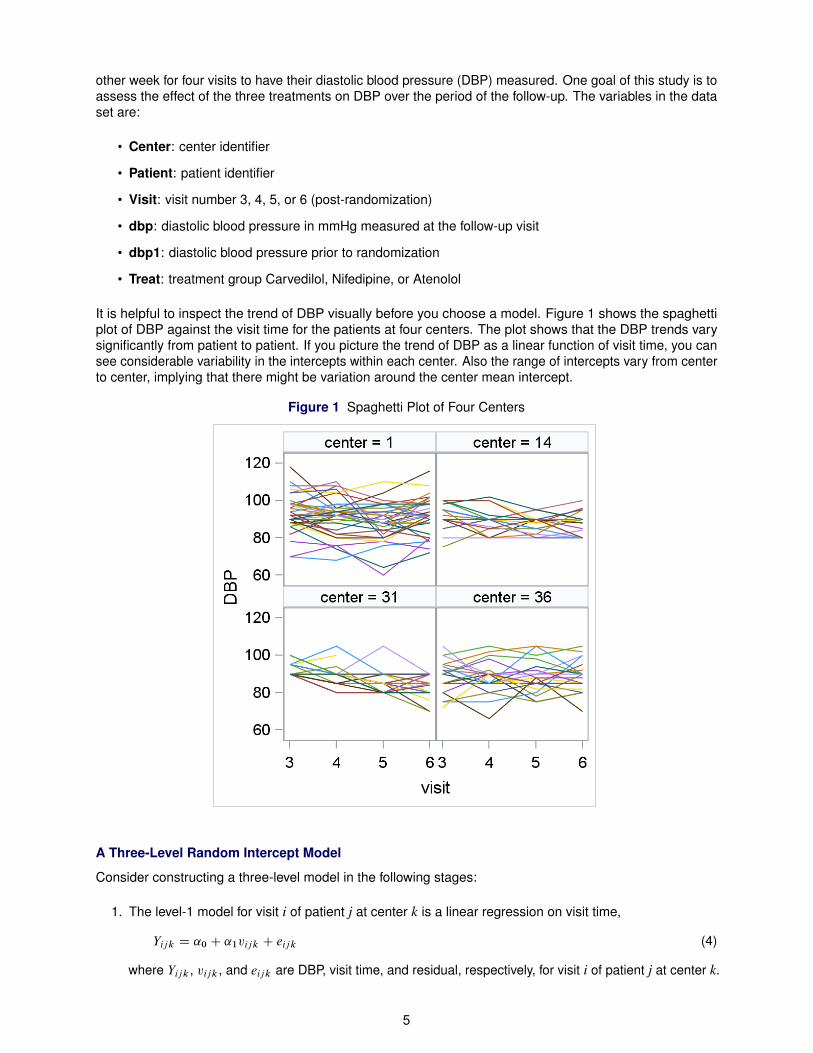
It is helpful to inspect the trend of DBP visually before you choose a model. Figure 1 shows the spaghettiplot of DBP against the visit time for the patients at four centers. The plot shows that the DBP trends varysignificantly from patient to patient. If you picture the trend of DBP as a linear function of visit time, you cansee considerable variability in the intercepts within each center. Also the range of intercepts vary from centerto center, implying that there might be variation around the center mean intercept.
Figure 1 Spaghetti Plot of Four Centers
A Three-Level Random Intercept Model
Consider constructing a three-level model in the following stages:
1. The level-1 model for visit i of patient j at center k is a linear regression on visit time,
Yijk D ˛0 C ˛1vijk C eijk (4)
where Yijk , vijk , and eijk are DBP, visit time, and residual, respectively, for visit i of patient j at center k.
5
2. Assume that the intercept ˛0 varies among patients according to the level-2 model,
˛0 D ˇ0 C ˇ1bjk C ˇ2�jk C pjk (5)
where bjk and �jk are level-2 covariates baseline DBP and treatment, respectively, and pjk is thepatient-level random intercept.
3. Express the variability among the centers in the level-3 model,
ˇ0 D �0 C ck (6)
where ck is the center-level random intercept.
Substituting the level-3 model into the level-2 model and then substituting the level-2 model into the level-1model yields
Yijk D �0 C ˛1vijk C eijk C
pjk C ˇ1bjk C ˇ2�jk C
ck
The following lines show part of the data set:
data mctrial;input patient visit center treat$ dbp dbp1;datalines;
79 3 1 Carvedil 96 10079 4 1 Carvedil 108 10080 3 1 Nifedipi 82 10080 4 1 Nifedipi 92 10080 5 1 Nifedipi 90 10080 6 1 Nifedipi 100 10081 3 1 Atenolol 86 100
... more lines ...
237 5 41 Atenolol 80 104237 6 41 Atenolol 90 104238 3 41 Nifedipi 88 112238 4 41 Nifedipi 100 112;
This model can be fit using the following PROC GLIMMIX code:
proc glimmix data=mctrial;class patient center treat;model dbp = dbp1 treat visit/solution;random intercept / subject = center;random intercept / subject = patient(center);covtest 'var(center) = 0' 0 .;covtest 'var(patient(center)) = 0' . 0;estimate 'Carvedil vs. Atenolol' treat 1 -1 0;estimate 'Carvedil vs. Nifedipi' treat 0 1 -1;
run;
The CLASS statement identifies categorical variables. You use the MODEL statement to specify all the fixedeffects, and you use one RANDOM statement for each level of clustering. In each RANDOM statement, therandom effects are followed by the SUBJECT= option, which identifies the level. You use the COVTESTstatement to make inferences about the covariance parameters. The two COVTEST statements here testwhether the variances of the patient-level random intercept and the center-level random intercept are zero,which is effectively a test for the significance for these random effects. Finally, the two ESTIMATE statementscompare the effect of the new treatment with the effects of the two standard ones.
6
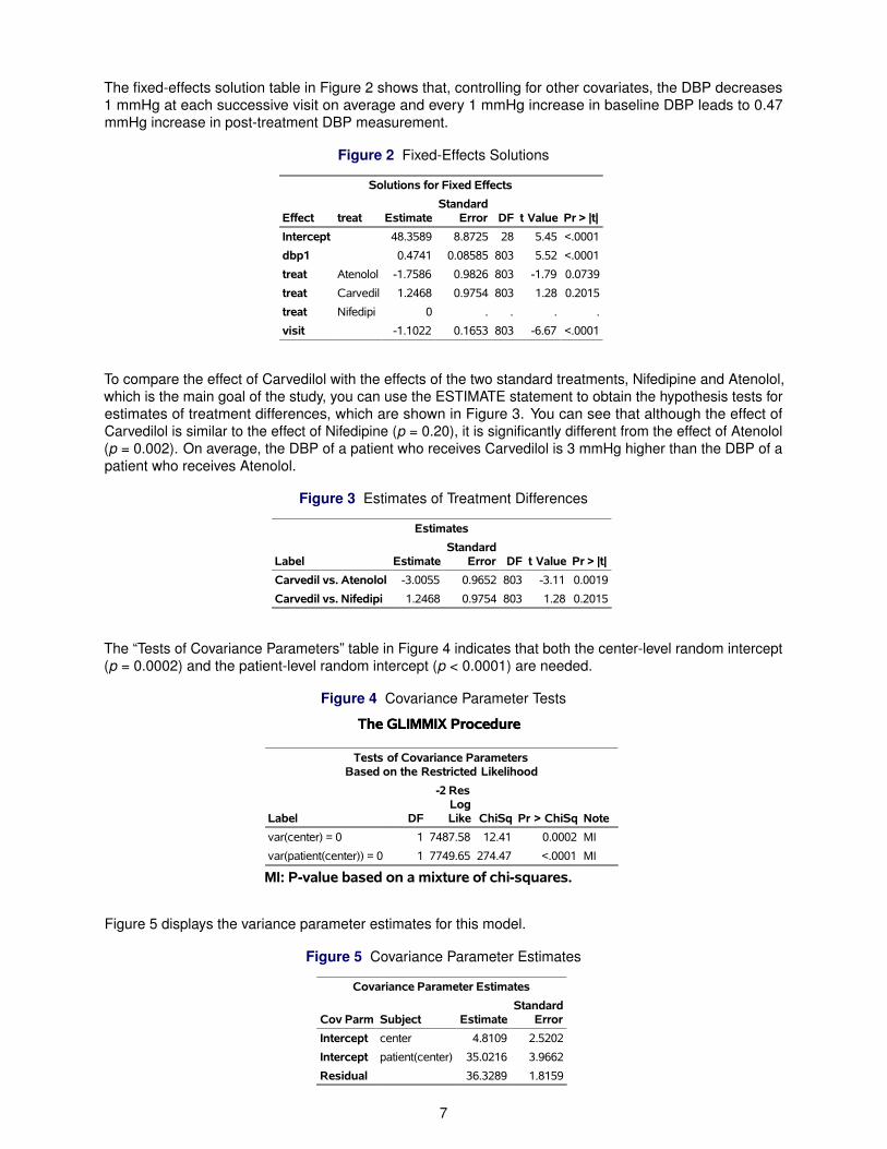
The fixed-effects solution table in Figure 2 shows that, controlling for other covariates, the DBP decreases1 mmHg at each successive visit on average and every 1 mmHg increase in baseline DBP leads to 0.47mmHg increase in post-treatment DBP measurement.
Figure 2 Fixed-Effects Solutions
Solutions for Fixed Effects
Effect treat EstimateStandard
Error DF t Value Pr > |t|
Intercept 48.3589 8.8725 28 5.45 <.0001
dbp1 0.4741 0.08585 803 5.52 <.0001
treat Atenolol -1.7586 0.9826 803 -1.79 0.0739
treat Carvedil 1.2468 0.9754 803 1.28 0.2015
treat Nifedipi 0 . . . .
visit -1.1022 0.1653 803 -6.67 <.0001
To compare the effect of Carvedilol with the effects of the two standard treatments, Nifedipine and Atenolol,which is the main goal of the study, you can use the ESTIMATE statement to obtain the hypothesis tests forestimates of treatment differences, which are shown in Figure 3. You can see that although the effect ofCarvedilol is similar to the effect of Nifedipine (p = 0.20), it is significantly different from the effect of Atenolol(p = 0.002). On average, the DBP of a patient who receives Carvedilol is 3 mmHg higher than the DBP of apatient who receives Atenolol.
Figure 3 Estimates of Treatment Differences
Estimates
Label EstimateStandard
Error DF t Value Pr > |t|
Carvedil vs. Atenolol -3.0055 0.9652 803 -3.11 0.0019
Carvedil vs. Nifedipi 1.2468 0.9754 803 1.28 0.2015
The “Tests of Covariance Parameters” table in Figure 4 indicates that both the center-level random intercept(p = 0.0002) and the patient-level random intercept (p < 0.0001) are needed.
Figure 4 Covariance Parameter Tests
The GLIMMIX ProcedureThe GLIMMIX Procedure
Tests of Covariance ParametersBased on the Restricted Likelihood
Label DF
-2 ResLogLike ChiSq Pr > ChiSq Note
var(center) = 0 1 7487.58 12.41 0.0002 MI
var(patient(center)) = 0 1 7749.65 274.47 <.0001 MI
MI: P-value based on a mixture of chi-squares.
Figure 5 displays the variance parameter estimates for this model.
Figure 5 Covariance Parameter Estimates
Covariance Parameter Estimates
Cov Parm Subject EstimateStandard
Error
Intercept center 4.8109 2.5202
Intercept patient(center) 35.0216 3.9662
Residual 36.3289 1.8159
7
Plugging the variance parameter estimates into equations (2) and (3), you can compute the conditionalcorrelation between DBP measurements of two different patients at the same center and the conditionalcorrelation between DBP measurements of two visits of the same patient as follows:
Corr.yijk ; yi 0j 0kjXk/ D4:8
4:8C 35C 36D 0:064 (7)
Corr.yijk ; yi 0jkjXk/ D4:8C 35
4:8C 35C 36D 0:53 (8)
In the preceding equations, Xk contains the visit-level and patient-level covariates for center k.
That is, of the variability in DBP that is not explained by the covariates, 6.4% is caused by unobservedcenter-specific attributes and 53% is caused by unobserved patient-specific attributes. Another way tointerpret this is that DBP measurements on the same patient are much more similar to each other than areDBP measurements on different patients at the same center, as the spaghetti plot in Figure 1 indicates.
Finally, using the estimated fixed effects and predicted random effects from the mixed model, you can returnfull circle to depict the elements of the multilevel model.
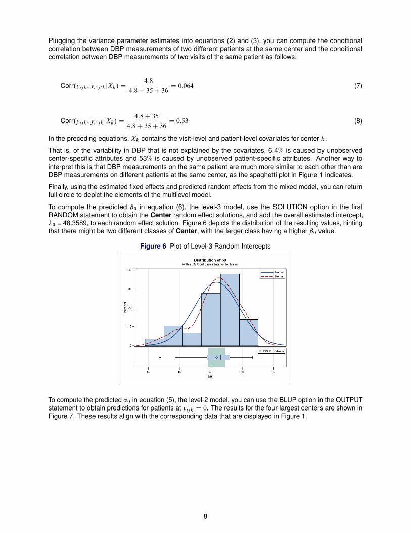
To compute the predicted ˇ0 in equation (6), the level-3 model, use the SOLUTION option in the firstRANDOM statement to obtain the Center random effect solutions, and add the overall estimated intercept,�0 = 48.3589, to each random effect solution. Figure 6 depicts the distribution of the resulting values, hintingthat there might be two different classes of Center, with the larger class having a higher ˇ0 value.
Figure 6 Plot of Level-3 Random Intercepts
To compute the predicted ˛0 in equation (5), the level-2 model, you can use the BLUP option in the OUTPUTstatement to obtain predictions for patients at vijk D 0. The results for the four largest centers are shown inFigure 7. These results align with the corresponding data that are displayed in Figure 1.
8
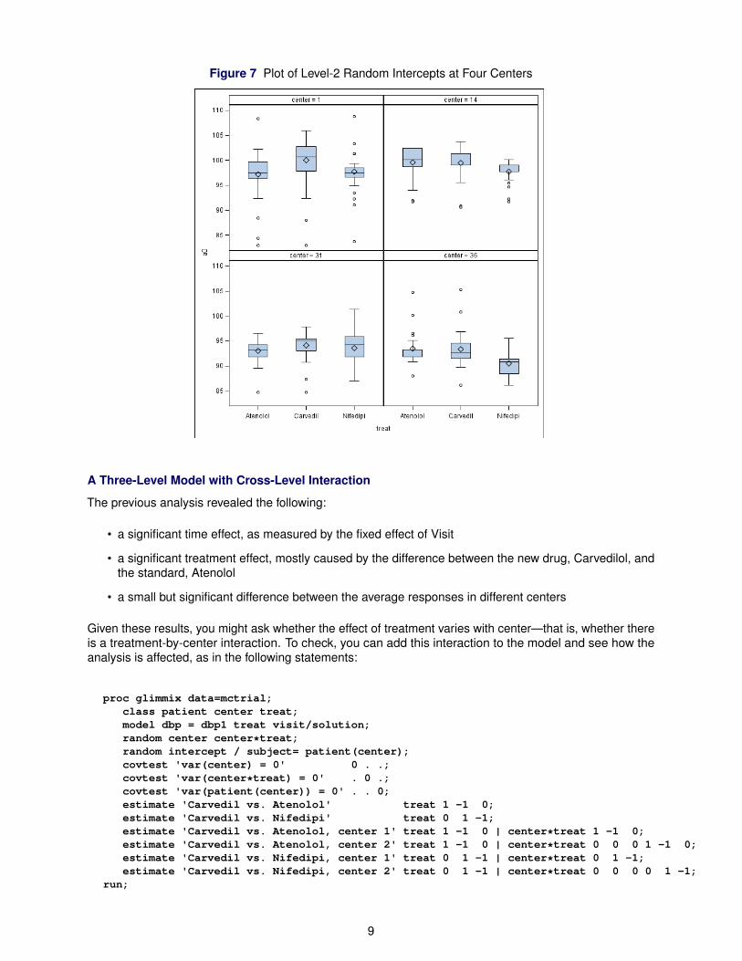
Figure 7 Plot of Level-2 Random Intercepts at Four Centers
A Three-Level Model with Cross-Level Interaction
The previous analysis revealed the following:
• a significant time effect, as measured by the fixed effect of Visit
• a significant treatment effect, mostly caused by the difference between the new drug, Carvedilol, andthe standard, Atenolol
• a small but significant difference between the average responses in different centers
Given these results, you might ask whether the effect of treatment varies with center—that is, whether thereis a treatment-by-center interaction. To check, you can add this interaction to the model and see how theanalysis is affected, as in the following statements:
proc glimmix data=mctrial;class patient center treat;model dbp = dbp1 treat visit/solution;random center center*treat;random intercept / subject= patient(center);covtest 'var(center) = 0' 0 . .;covtest 'var(center*treat) = 0' . 0 .;covtest 'var(patient(center)) = 0' . . 0;estimate 'Carvedil vs. Atenolol' treat 1 -1 0;estimate 'Carvedil vs. Nifedipi' treat 0 1 -1;estimate 'Carvedil vs. Atenolol, center 1' treat 1 -1 0 | center*treat 1 -1 0;estimate 'Carvedil vs. Atenolol, center 2' treat 1 -1 0 | center*treat 0 0 0 1 -1 0;estimate 'Carvedil vs. Nifedipi, center 1' treat 0 1 -1 | center*treat 0 1 -1;estimate 'Carvedil vs. Nifedipi, center 2' treat 0 1 -1 | center*treat 0 0 0 0 1 -1;
run;
9
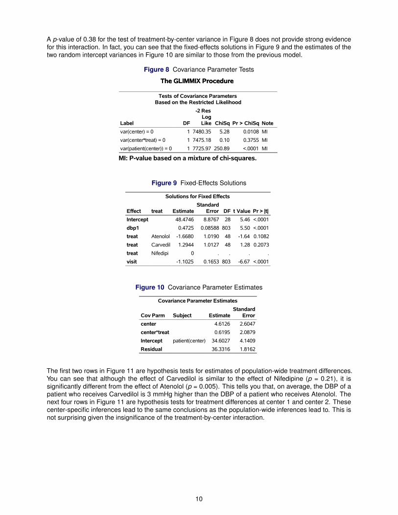
A p-value of 0.38 for the test of treatment-by-center variance in Figure 8 does not provide strong evidencefor this interaction. In fact, you can see that the fixed-effects solutions in Figure 9 and the estimates of thetwo random intercept variances in Figure 10 are similar to those from the previous model.
Figure 8 Covariance Parameter Tests
The GLIMMIX ProcedureThe GLIMMIX Procedure
Tests of Covariance ParametersBased on the Restricted Likelihood
Label DF
-2 ResLogLike ChiSq Pr > ChiSq Note
var(center) = 0 1 7480.35 5.28 0.0108 MI
var(center*treat) = 0 1 7475.18 0.10 0.3755 MI
var(patient(center)) = 0 1 7725.97 250.89 <.0001 MI
MI: P-value based on a mixture of chi-squares.
Figure 9 Fixed-Effects Solutions
Solutions for Fixed Effects
Effect treat EstimateStandard
Error DF t Value Pr > |t|
Intercept 48.4746 8.8767 28 5.46 <.0001
dbp1 0.4725 0.08588 803 5.50 <.0001
treat Atenolol -1.6680 1.0190 48 -1.64 0.1082
treat Carvedil 1.2944 1.0127 48 1.28 0.2073
treat Nifedipi 0 . . . .
visit -1.1025 0.1653 803 -6.67 <.0001
Figure 10 Covariance Parameter Estimates
Covariance Parameter Estimates
Cov Parm Subject EstimateStandard
Error
center 4.6126 2.6047
center*treat 0.6195 2.0879
Intercept patient(center) 34.6027 4.1409
Residual 36.3316 1.8162
The first two rows in Figure 11 are hypothesis tests for estimates of population-wide treatment differences.You can see that although the effect of Carvedilol is similar to the effect of Nifedipine (p = 0.21), it issignificantly different from the effect of Atenolol (p = 0.005). This tells you that, on average, the DBP of apatient who receives Carvedilol is 3 mmHg higher than the DBP of a patient who receives Atenolol. Thenext four rows in Figure 11 are hypothesis tests for treatment differences at center 1 and center 2. Thesecenter-specific inferences lead to the same conclusions as the population-wide inferences lead to. This isnot surprising given the insignificance of the treatment-by-center interaction.
10
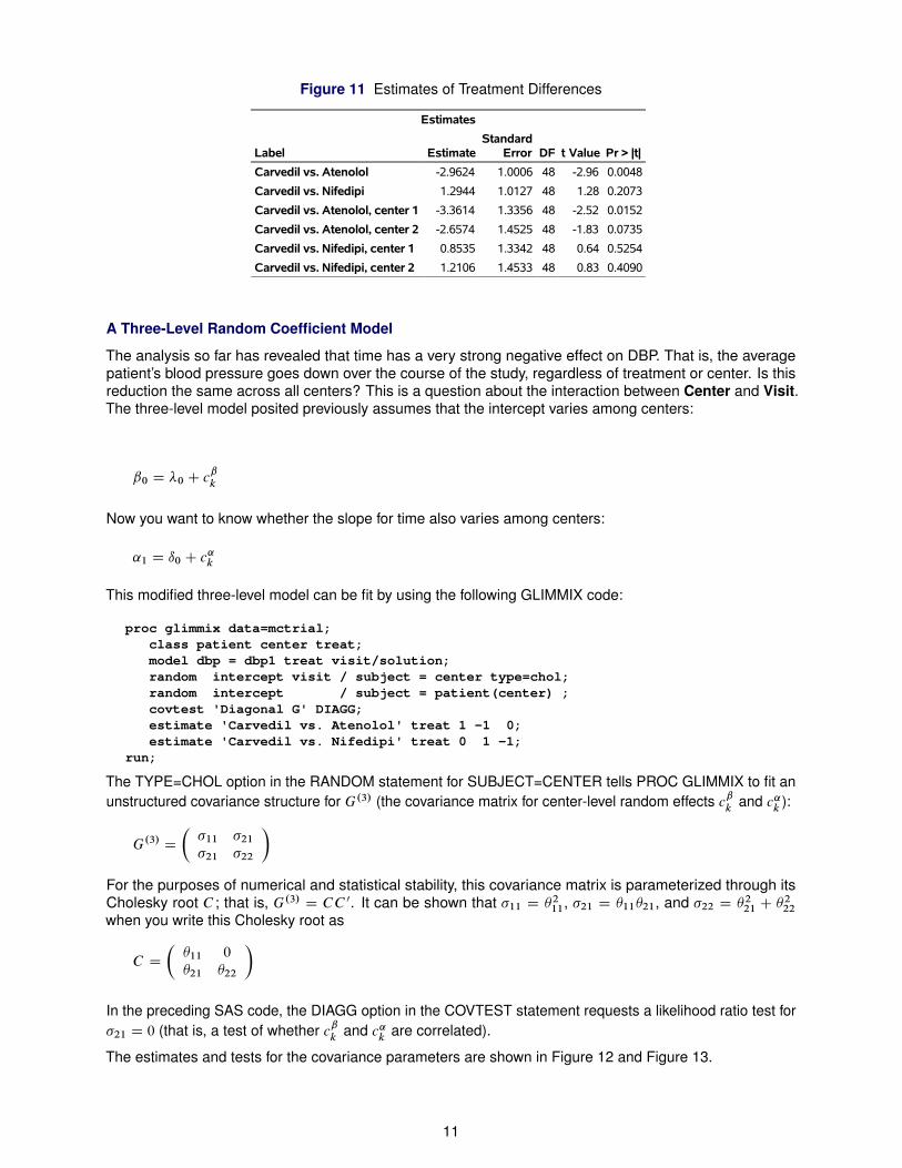
Figure 11 Estimates of Treatment Differences
Estimates
Label EstimateStandard
Error DF t Value Pr > |t|
Carvedil vs. Atenolol -2.9624 1.0006 48 -2.96 0.0048
Carvedil vs. Nifedipi 1.2944 1.0127 48 1.28 0.2073
Carvedil vs. Atenolol, center 1 -3.3614 1.3356 48 -2.52 0.0152
Carvedil vs. Atenolol, center 2 -2.6574 1.4525 48 -1.83 0.0735
Carvedil vs. Nifedipi, center 1 0.8535 1.3342 48 0.64 0.5254
Carvedil vs. Nifedipi, center 2 1.2106 1.4533 48 0.83 0.4090
A Three-Level Random Coefficient Model
The analysis so far has revealed that time has a very strong negative effect on DBP. That is, the averagepatient’s blood pressure goes down over the course of the study, regardless of treatment or center. Is thisreduction the same across all centers? This is a question about the interaction between Center and Visit.The three-level model posited previously assumes that the intercept varies among centers:
ˇ0 D �0 C cˇ
k
Now you want to know whether the slope for time also varies among centers:
˛1 D ı0 C c˛k
This modified three-level model can be fit by using the following GLIMMIX code:
proc glimmix data=mctrial;class patient center treat;model dbp = dbp1 treat visit/solution;random intercept visit / subject = center type=chol;random intercept / subject = patient(center) ;covtest 'Diagonal G' DIAGG;estimate 'Carvedil vs. Atenolol' treat 1 -1 0;estimate 'Carvedil vs. Nifedipi' treat 0 1 -1;
run;
The TYPE=CHOL option in the RANDOM statement for SUBJECT=CENTER tells PROC GLIMMIX to fit anunstructured covariance structure for G.3/ (the covariance matrix for center-level random effects cˇ
kand c˛
k):
G.3/ D
��11 �21�21 �22
�For the purposes of numerical and statistical stability, this covariance matrix is parameterized through itsCholesky root C ; that is, G.3/ D CC 0. It can be shown that �11 D �211, �21 D �11�21, and �22 D �221 C �
222
when you write this Cholesky root as
C D
��11 0
�21 �22
�
In the preceding SAS code, the DIAGG option in the COVTEST statement requests a likelihood ratio test for�21 D 0 (that is, a test of whether cˇ
kand c˛
kare correlated).
The estimates and tests for the covariance parameters are shown in Figure 12 and Figure 13.
11
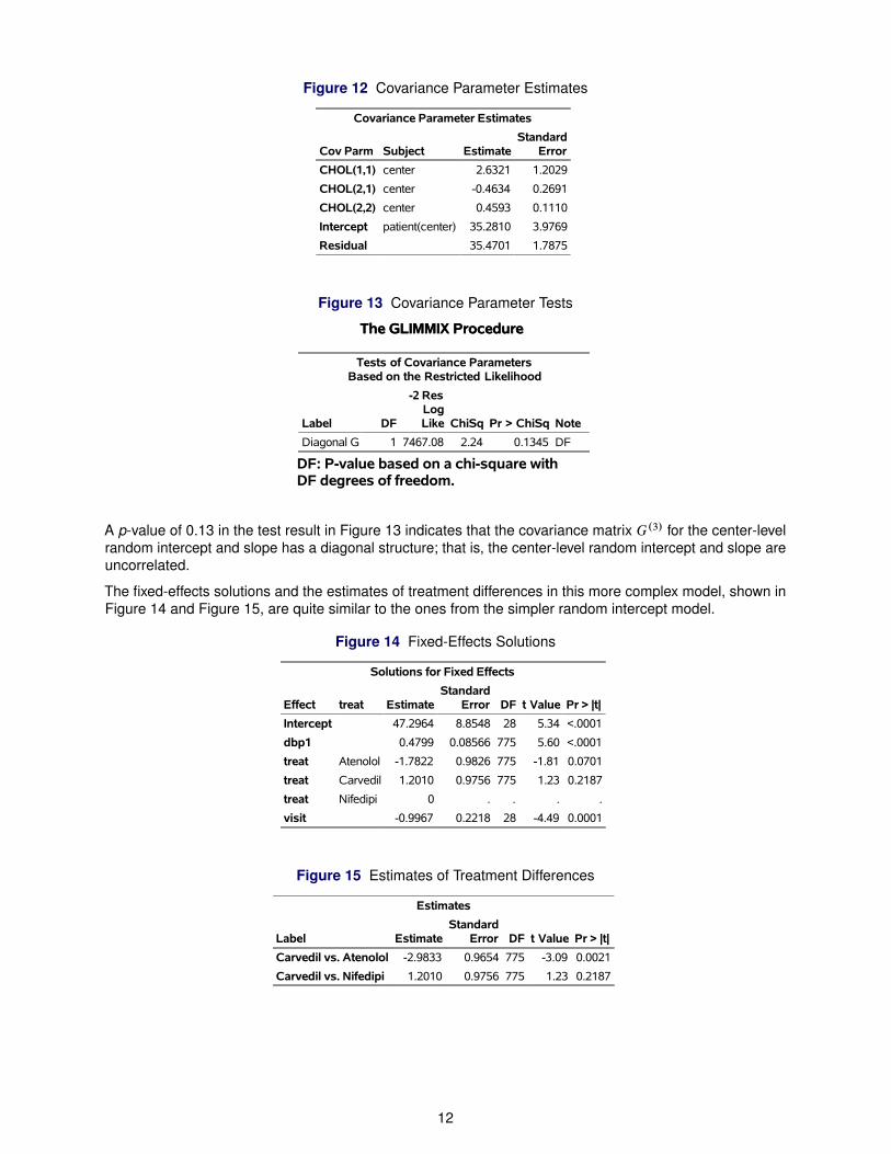
Figure 12 Covariance Parameter Estimates
Covariance Parameter Estimates
Cov Parm Subject EstimateStandard
Error
CHOL(1,1) center 2.6321 1.2029
CHOL(2,1) center -0.4634 0.2691
CHOL(2,2) center 0.4593 0.1110
Intercept patient(center) 35.2810 3.9769
Residual 35.4701 1.7875
Figure 13 Covariance Parameter Tests
The GLIMMIX ProcedureThe GLIMMIX Procedure
Tests of Covariance ParametersBased on the Restricted Likelihood
Label DF
-2 ResLogLike ChiSq Pr > ChiSq Note
Diagonal G 1 7467.08 2.24 0.1345 DF
DF: P-value based on a chi-square withDF degrees of freedom.
A p-value of 0.13 in the test result in Figure 13 indicates that the covariance matrix G.3/ for the center-levelrandom intercept and slope has a diagonal structure; that is, the center-level random intercept and slope areuncorrelated.
The fixed-effects solutions and the estimates of treatment differences in this more complex model, shown inFigure 14 and Figure 15, are quite similar to the ones from the simpler random intercept model.
Figure 14 Fixed-Effects Solutions
Solutions for Fixed Effects
Effect treat EstimateStandard
Error DF t Value Pr > |t|
Intercept 47.2964 8.8548 28 5.34 <.0001
dbp1 0.4799 0.08566 775 5.60 <.0001
treat Atenolol -1.7822 0.9826 775 -1.81 0.0701
treat Carvedil 1.2010 0.9756 775 1.23 0.2187
treat Nifedipi 0 . . . .
visit -0.9967 0.2218 28 -4.49 0.0001
Figure 15 Estimates of Treatment Differences
Estimates
Label EstimateStandard
Error DF t Value Pr > |t|
Carvedil vs. Atenolol -2.9833 0.9654 775 -3.09 0.0021
Carvedil vs. Nifedipi 1.2010 0.9756 775 1.23 0.2187
12
WEIGHTED MULTILEVEL MODELS
Multistage Sampling Surveys and Multilevel Models
An important example of multilevel data for which specialized analytic techniques are required is datathat arise from multistage survey sampling. In a multistage sampling design, you first select a sampleof large clusters of observations. The observations in this sample are called the primary sampling units(PSU). Then, from each sampled PSU, you select a sample of smaller clusters. These observations arecalled the secondary sampling units (SSU). Then, from each sampled SSU, you select a sample of evensmaller clusters or observation units. You continue this process down to the individual units for which surveyresponses are measured. For example, if you want to survey all school children in your state, you mightfirst sample the districts in the state, then sample some schools within each selected district, then samplesome classes within each selected school, and finally sample students within each selected class. It is alsocommon to select all the units at any particular stage as your sample at that stage—for example, surveyingall the students in the selected classes.
Multilevel modeling is naturally appropriate for data that arise from a multistage sample. Often, the hierarchicalclusters of the sampling design map directly to the hierarchical random effects in the multilevel model, andthe characteristics of the units at each stage become level-specific explanatory variables.
The key point is how you handle the multistage sampling weights. Survey weights are often derivedby quite sophisticated methods to account for such desirable survey features as rational oversampling,poststratification, nonresponse, and so on. If you have survey weights available at every stage of the surveydesign, then you need to take these weights into account properly in order to draw valid inferences aboutyour population of interest. The WEIGHT statement in PROC GLIMMIX scales the residual covariancematrix; it does not supply multiple levels of frequency weights.
SAS/STAT 13.1 to the rescue! New in this release of PROC GLIMMIX are the OBSWEIGHT= option in theMODEL statement and the WEIGHT= option in the RANDOM statement, which enable you to specify justsuch multiple levels of weights. This is the key feature that you can use in PROC GLIMMIX to fit multilevelmodels to multistage survey samples. The next section discusses the underlying general methodology forcomputing estimates and their variances in weighted multilevel models. An example in a subsequent sectionshows you how to do this in practice with a multistage survey sample of the Programme for InternationalStudent Assessment (PISA) study.
Not Quite Maximum Likelihood Estimation
The basic estimation principle that you use in analyzing multistage samples with multilevel models is thefundamental statistical technique of maximum likelihood, but there is a terminological tangle:
• On one hand, with a survey sample you don’t actually have the likelihood that you want to be able tomaximize: the one for the entire population. So you use the weighted likelihood as an estimate for thepopulation likelihood, and you hope that by maximizing the former you get close to the maximum ofthe latter. This weighted likelihood is called the pseudolikelihood by survey samplers. To compute theweighted likelihood, you use the METHOD=QUADRATURE option.
• On the other hand, if the responses in your multistage sample are nonnormal, then it is not possible towrite down the likelihood for the corresponding generalized linear mixed models. In PROC GLIMMIX,you can use adaptive quadrature (METHOD=QUADRATURE) to approximate the likelihood or you canuse an approximation that is based on linearization. The likelihood for the linearized model is alsocalled the pseudolikelihood by generalized linear mixed modelers, but they sometimes also refer to itas the quasilikelihood. It should not be confused with the pseudolikelihood that is computed for theweighted multilevel models.
To illustrate the computation of the weighted likelihood, consider the following three-stage sampling design.(Extending this example to models that have more than three levels is straightforward.) Let superscript.l/ denote the lth level and n.l/ denote the number of level-l units in the sample. Also let i D 1; : : : ; n
.1/j ,
j D 1; : : : n.2/
k, and k D 1; : : : n.3/ denote the indices of units at level 1, level 2, and level 3, respectively.
Assume that the first-stage cluster (level-3 unit) k is selected with probability �k , the second-stage cluster
13

(level-2 unit) j is selected with probability �j jk (which is the conditional probability that the second-stagecluster j is selected given that the first-stage cluster k is already selected in the sample), and the third-stageunit (level-1 unit) i is selected with probability �i jjk (which is the conditional probability that the third-stageunit i is selected given that the second-stage cluster j within the first-stage cluster k is already selected inthe sample).
If you use the inverse selection probability weights wj jk D 1=�j jk and wi jjk D 1=�i jjk, a sample-basedestimator for the conditional log likelihood contribution of the first-stage cluster k is
log .p.ykj .2/
k; .3/
k// D
n.2/
kXjD1
wj jk
n.1/
jXiD1
wi jjk log .p.yijkj .2/
jk; .3/
k//
where .2/jk
is the random-effects vector for the second-stage cluster j within first-stage cluster k, .2/kD
. .2/
1k; .2/
2k; : : : ;
.2/
n.2/
kk/, and .3/
kis the random-effects vector for the first-stage cluster k.
As with unweighted multilevel models, the adaptive quadrature method is used to compute the likelihoodcontribution of the first-stage cluster k:
p.yk/ D
Zp.ykj
.2/
k; .3/
k/p.
.2/
k/p.
.3/
k/d.
.2/
k/d.
.3/
k/
A sample-based estimator for the population log likelihood is
log .p.y// Dn.3/XkD1
wk log .p.yk//
where wk D 1=�k .
Robust Standard Error Estimator
For inference about fixed effects and variances that are estimated by the likelihood method discussedpreviously, you can use the empirical (sandwich) variance estimators.
The only empirical estimator that PROC GLIMMIX computes in SAS/STAT 13.2 for weighted multilevelmodels is EMPIRICAL=CLASSICAL, which can be described as follows.
Let ˛ D .ˇ0; � 0/0, where ˇ is the vector of the fixed-effects parameters and � is the vector of covarianceparameters. For an L-level model, Rabe-Hesketh and Skrondal (2006) show that the gradient can be writtenas a weighted sum of the gradients of the top-level units,
n.L/XkD1
wk@ log.p.yk I˛//
@˛�
n.L/XkD1
Sk.˛/
where n.L/ is the number of level-L units and Sk.˛/ is the weighted score vector of the level-L unit k. Theestimator of the “meat” of the sandwich estimator can be written as
J Dn.L/
n.L/ � 1
n.L/XkD1
Sk. O /Sk. O /0
The empirical estimator of the covariance matrix of O can be constructed as
H. O /�1JH. O /�1
where H.˛/ is the second derivative matrix of the log pseudolikelihood with respect to ˛:
H.˛/ D@2 log.p.yk I˛//
@˛@˛0
The covariance parameter estimators that are obtained by the weighted likelihood method can be biasedwhen the sample size is small. Pfeffermann et al. (1998) and Rabe-Hesketh and Skrondal (2006) discuss
14

two weight-scaling methods for reducing the biases of the covariance parameter estimators in a two-levelmodel. To derive the scaling factor � for a two-level model, let ni denote the number of level-1 units in thelevel-2 unit i and let wj ji denote the weight of level-1 unit j in level-2 unit i. The first method computes an“apparent” cluster size as the “effective” sample size:
niXjD1
�wj ji D.Pni
jD1wj ji /2Pni
jD1w2j ji
Therefore, the scale factor is
� D
Pni
jD1wj jiPni
jD1w2j ji
The second method sets the apparent cluster size equal to the actual cluster size so that the scale factor is
� DniPni
jD1wj ji
The level-1 scaled weights are then computed as wsj jiD �wj ji . PROC GLIMMIX directly uses the weights
that are provided in the data set. To use the scaled weights, you need to provide them in the data set.
Example 2: The Programme for International Student Assessment (PISA) Study
Rabe-Hesketh and Skrondal (2006) introduce the data about reading proficiency among 15-year-old Ameri-can students from the PISA study. This section shows you how to use PROC GLIMMIX to fit a weightedmultilevel model to this data. The PISA study has a three-stage sampling design: geographic areas (PSUs)are sampled at stage 1, schools are sampled at stage 2, and students are sampled at stage 3. Samplingprobabilities are devised at each stage of the study by using criteria that account for estimated sizes andpercentages of minority students. Because of nonresponse and missingness on some of the covariates,2,069 students from 148 schools in 46 PSUs are included in the analysis. The student-level and school-levelweights (wfstuwt and wnrschbw, respectively) are inverse probabilities that are further adjusted for non-response and noninclusion. To reduce the bias in the variance parameter estimate, scaled student-levelweights (sw1) are computed using Method 1 in Pfeffermann et al. (1998) and Rabe-Hesketh and Skrondal(2006).
The outcome considered here is the binary variable Passread. This variable takes the value 1 when thereading proficiency is at the top two levels that are defined by the Organization for Economic Co-operationand Development. The variable Idschool identifies the schools. The explanatory variables in the data setare:
• Female indicates whether the student is female.
• ISEI indicates the student’s international socioeconomic index.
• Highschool indicates whether the highest education level by either parent is high school.
• College indicates whether the highest education level by either parent is college.
• Testlang indicates whether the test language (English) is spoken at home.
• Onefor indicates whether one parent is foreign-born.
• Bothfor indicates whether both parents are foreign-born.
• MISEI indicates the school mean ISEI.
Of these eight variables, MISEI is a school-level covariate and the rest are student-level covariates. Theschool mean ISEI is included in the model to check the between-school effect of ISEI. Including the MISEIvariable enables you to consider the effect of the socioeconomic mix of a school on a student’s readingproficiency. The following lines show part of the data set:
15
data pisa;input sw1 misei wnrschbw female isei highschool college onefor
bothfor testlang passread idschool;datalines;
1.000 48.3 146.02 1 37 0 1 1 0 1 1 11.000 48.3 146.02 1 77 1 0 0 0 1 1 11.000 48.3 146.02 1 53 0 1 0 0 1 0 11.000 48.3 146.02 1 30 1 0 0 0 1 0 11.000 48.3 146.02 1 70 0 1 0 0 1 0 11.000 48.3 146.02 1 39 0 1 0 0 1 1 1
... more lines ...
0.962 40.5 140.92 0 69 0 1 0 0 1 0 1511.100 40.5 140.92 1 43 0 1 0 0 1 0 1510.962 40.5 140.92 0 23 1 0 0 0 1 0 1510.962 40.5 140.92 0 23 0 1 0 0 1 0 151;
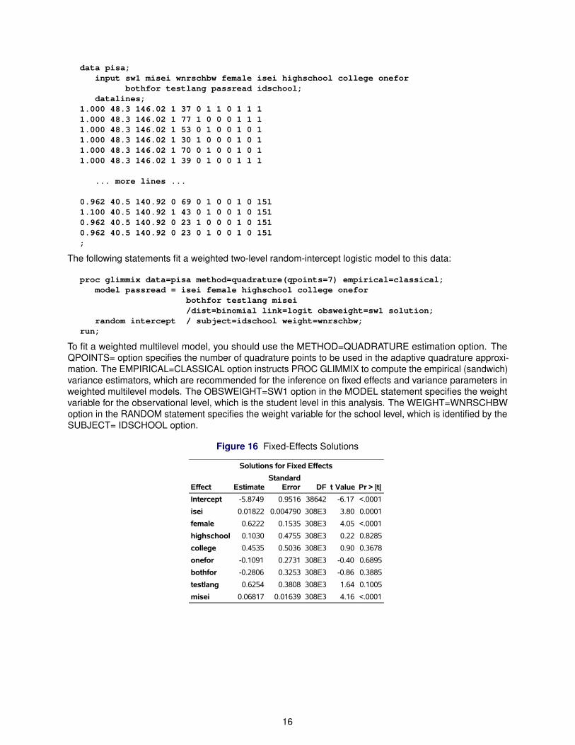
The following statements fit a weighted two-level random-intercept logistic model to this data:
proc glimmix data=pisa method=quadrature(qpoints=7) empirical=classical;model passread = isei female highschool college onefor
bothfor testlang misei/dist=binomial link=logit obsweight=sw1 solution;
random intercept / subject=idschool weight=wnrschbw;run;
To fit a weighted multilevel model, you should use the METHOD=QUADRATURE estimation option. TheQPOINTS= option specifies the number of quadrature points to be used in the adaptive quadrature approxi-mation. The EMPIRICAL=CLASSICAL option instructs PROC GLIMMIX to compute the empirical (sandwich)variance estimators, which are recommended for the inference on fixed effects and variance parameters inweighted multilevel models. The OBSWEIGHT=SW1 option in the MODEL statement specifies the weightvariable for the observational level, which is the student level in this analysis. The WEIGHT=WNRSCHBWoption in the RANDOM statement specifies the weight variable for the school level, which is identified by theSUBJECT= IDSCHOOL option.
Figure 16 Fixed-Effects Solutions
Solutions for Fixed Effects
Effect EstimateStandard
Error DF t Value Pr > |t|
Intercept -5.8749 0.9516 38642 -6.17 <.0001
isei 0.01822 0.004790 308E3 3.80 0.0001
female 0.6222 0.1535 308E3 4.05 <.0001
highschool 0.1030 0.4755 308E3 0.22 0.8285
college 0.4535 0.5036 308E3 0.90 0.3678
onefor -0.1091 0.2731 308E3 -0.40 0.6895
bothfor -0.2806 0.3253 308E3 -0.86 0.3885
testlang 0.6254 0.3808 308E3 1.64 0.1005
misei 0.06817 0.01639 308E3 4.16 <.0001
16
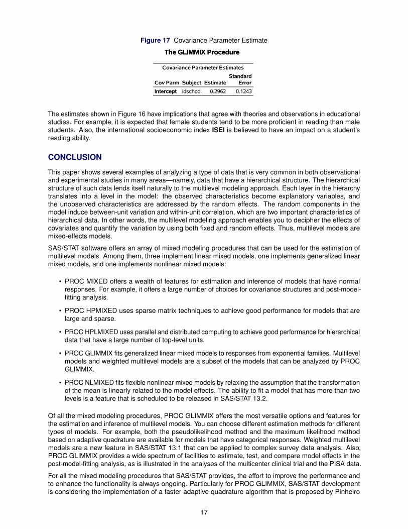
Figure 17 Covariance Parameter Estimate
The GLIMMIX ProcedureThe GLIMMIX Procedure
Covariance Parameter Estimates
Cov Parm Subject EstimateStandard
Error
Intercept idschool 0.2962 0.1243
The estimates shown in Figure 16 have implications that agree with theories and observations in educationalstudies. For example, it is expected that female students tend to be more proficient in reading than malestudents. Also, the international socioeconomic index ISEI is believed to have an impact on a student’sreading ability.
CONCLUSION
This paper shows several examples of analyzing a type of data that is very common in both observationaland experimental studies in many areas—namely, data that have a hierarchical structure. The hierarchicalstructure of such data lends itself naturally to the multilevel modeling approach. Each layer in the hierarchytranslates into a level in the model: the observed characteristics become explanatory variables, andthe unobserved characteristics are addressed by the random effects. The random components in themodel induce between-unit variation and within-unit correlation, which are two important characteristics ofhierarchical data. In other words, the multilevel modeling approach enables you to decipher the effects ofcovariates and quantify the variation by using both fixed and random effects. Thus, multilevel models aremixed-effects models.
SAS/STAT software offers an array of mixed modeling procedures that can be used for the estimation ofmultilevel models. Among them, three implement linear mixed models, one implements generalized linearmixed models, and one implements nonlinear mixed models:
• PROC MIXED offers a wealth of features for estimation and inference of models that have normalresponses. For example, it offers a large number of choices for covariance structures and post-model-fitting analysis.
• PROC HPMIXED uses sparse matrix techniques to achieve good performance for models that arelarge and sparse.
• PROC HPLMIXED uses parallel and distributed computing to achieve good performance for hierarchicaldata that have a large number of top-level units.
• PROC GLIMMIX fits generalized linear mixed models to responses from exponential families. Multilevelmodels and weighted multilevel models are a subset of the models that can be analyzed by PROCGLIMMIX.
• PROC NLMIXED fits flexible nonlinear mixed models by relaxing the assumption that the transformationof the mean is linearly related to the model effects. The ability to fit a model that has more than twolevels is a feature that is scheduled to be released in SAS/STAT 13.2.
Of all the mixed modeling procedures, PROC GLIMMlX offers the most versatile options and features forthe estimation and inference of multilevel models. You can choose different estimation methods for differenttypes of models. For example, both the pseudolikelihood method and the maximum likelihood methodbased on adaptive quadrature are available for models that have categorical responses. Weighted multilevelmodels are a new feature in SAS/STAT 13.1 that can be applied to complex survey data analysis. Also,PROC GLIMMIX provides a wide spectrum of facilities to estimate, test, and compare model effects in thepost-model-fitting analysis, as is illustrated in the analyses of the multicenter clinical trial and the PISA data.
For all the mixed modeling procedures that SAS/STAT provides, the effort to improve the performance andto enhance the functionality is always ongoing. Particularly for PROC GLIMMIX, SAS/STAT developmentis considering the implementation of a faster adaptive quadrature algorithm that is proposed by Pinheiro
17
and Chao (2006). It is well known that the quadrature approximation is computationally intensive for modelsthat have large numbers of units and random effects at lower levels. This new algorithm will significantlyreduce the computation burden and thus improve the performance. Also, it is worth mentioning that thecorrelation estimates in equations (2) and (3) can potentially be reused for designing the next blood pressurestudy, using methods discussed in Castelloe (2014). Outliers are a common concern in multilevel models asthey are in other regression models. Multilevel model designs have multiple levels of observations and thusmultiple levels of outliers. These outliers can potentially be studied with the scaled Cook’s distance ideas ofZhu, Ibrahim, and Cho (2012), using the SAS implementation discussed in Schneider and Tobias (2014).
REFERENCES
Brown, H. and Prescott, R. (1999), Applied Mixed Models in Medicine, New York: John Wiley & Sons.
Castelloe, J. (2014), “Power and Sample Size for MANOVA and Repeated Measures with the GLMPOWERProcedure,” in Proceedings of the SAS Global Forum 2014 Conference, Cary, NC: SAS Institute Inc.URL http://support.sas.com/resources/papers/proceedings14/SAS030-2014.pdf
Littell, R. C., Milliken, G. A., Stroup, W. W., and Wolfinger, R. D. (1996), SAS System for Mixed Models, Cary,NC: SAS Institute Inc.
Pfeffermann, D., Skinner, C. J., Holmes, D. J., Goldstein, H., and Rasbash, J. (1998), “Weighting for UnequalSelection Probabilities in Multilevel Models,” Journal of the Royal Statistical Society, Series B, 60, 23–40.
Pinheiro, J. C. and Chao, E. C. (2006), “Efficient Laplacian and Adaptive Gaussian Quadrature Algorithmsfor Multilevel Generalized Linear Mixed Models,” Journal of Computational and Graphical Statistics, 15,58–81.
Rabe-Hesketh, S. and Skrondal, A. (2006), “Multilevel Modelling of Complex Survey Data,” Journal of theRoyal Statistical Society, Series A, 169, 805–827.
Schneider, G. and Tobias, R. D. (2014), “A SAS Macro to Diagnose Influential Subjects in LongitudinalStudies,” in Proceedings of the SAS Global Forum 2014 Conference, Cary, NC: SAS Institute Inc.URL http://support.sas.com/resources/papers/proceedings14/1461-2014.pdf
Zhu, H., Ibrahim, J. G., and Cho, H. (2012), “Perturbation and Scaled Cook’s Distance,” Annals of Statistics,40, 785–811.
ACKNOWLEDGMENTS
The author is grateful to Randy Tobias, Pushpal Mukhopadhyay, Tianlin Wang, Anne Baxter, Tim Arnold,and Ed Huddleston of the Advanced Analytics Division, and Kathleen Kiernan and Jill Tao of the TechnicalSupport Division at SAS Institute Inc. for their valuable assistance in the preparation of this manuscript.
CONTACT INFORMATION
Your comments and questions are valued and encouraged. Contact the author:
Min ZhuSAS Institute Inc.SAS Campus DriveCary, NC [email protected]
18