analyzing lasik optical data using zernike functions

� MATLAB Digest www.mathworks.com TM

Frits Zernike (�888 – �966)

Frederik (Frits) Zernike was born in Amsterdam on July 16,

1888. He graduated with a doctorate in chemistry from the

University of Amsterdam in 1915. That same year, Zernike

became a lecturer in physics at the University of Groningen,

becoming a full professor in 1920.

For the next decade, Zernike focused his research on statistical

mechanics, turning to optics in the 1930s. He invented phase

contrast microscopy, a technique that exploits the phase differences

produced by different materials or tissues when diffracting light.

These phase differences, which cause changes in intensity, can be

used to image living tissue without having to use dyes or stains.

Zernike received a patent for this invention in 1936, and was

awarded the Nobel Prize in 1953. His numerous other awards

and honors, including an honorary doctorate in Medicine from the

University of Amsterdam and the Rumford Medal from the Royal

Society in 1952. He became a Fellow of the Royal Society in 1956.

Researchers in fields as diverse as optometry,

astronomy, and photonics face a common

challenge: how to accurately measure structural de-

formations in circular optical elements such as ocular

lenses or corneas (in optometry), mirrors (in astronomy)

or optical fibers (in photonics), or the aberrations in

optical wavefronts caused by these deformations.

In optical systems, both the measurement devices, which are con-structed using lenses, optical fibers, or other optical components, and the subjects being measured, such as a patient’s eye or a telescope mir-ror, are often circular. As a result, measurement data is usually ex-pressed over a circular domain. When researchers need to characterize the structure of measured deformations and aberrations using Fourier analysis, they most often use Zernike functions, because these form a complete, orthogonal basis over the unit circle.

Using pre- and post-operative corneal topography data from a LASIK surgery patient as an example, this article describes the modal analysis of optics data using Zernike functions implemented in MATLAB®. Using these M-Files, the spectrum of Zernike modal amplitudes can be computed with a few simple lines of MATLAB code. The functions used in this article are available for download on MATLAB Central.

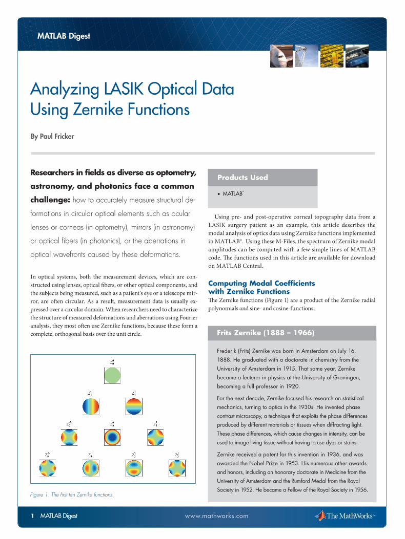
Computing Modal Coefficients with Zernike FunctionsThe Zernike functions (Figure 1) are a product of the Zernike radial polynomials and sine- and cosine-functions,

By Paul Fricker

Analyzing LASIK Optical Data Using Zernike Functions

MATLAB Digest

Products Used ■ MATLAB®

Figure 1. The first ten Zernike functions.


Equation 1

The index n = 0,1,2,… is called the degree of the function or polyno-mial, while m = -n to +n, with (n-m) even, is called the order. The ra-dial polynomials are usually defined using their series representation as a finite sum of powers of r2:

Although this expression looks complicated, the Rnm(r) are, in fact,

simple polynomials (Table 1). The first 10 Zernike functions, evaluated using equation 1, are listed in Table 2. The low mode number functions are used so frequently for analyzing optical data that many are given common names.

R00(r) 1

R11(r) r

R20(r) 2r2 – 1

R22(r) r2

R31(r) 3r3 – 2r

R33(r) r3

Table 1. The first six Zernike radial polynomials.

Z00(r,θ) 1

Z1-1(r,θ) rcosθ x-tilt

Z11(r,θ) rsinθ y-tilt

Z2-2(r,θ) r2 cos 2θ astigmatism

Z20(r, θ) 2r2 – 1 defocus

Z22(r, θ) r2 sin 2θ astigmatism

Z3-3(r, θ) r3 cos 3θ trefoil

Z3-1(r, θ) (3r3 – 2r) cos θ coma

Z31(r, θ) (3r3 – 2r) sin θ coma

Z33(r, θ) r3 sin 3θ trefoil

Table 2. The first ten Zernike radial functions and their common names.

These functions are useful as a basis for decomposing complex func-tions or data because they are orthogonal over the unit circle, meaning that they satisfy the following relation:

The factor (2n + 1)-1 on the right is usually used as a normalization constant for the functions. Using this orthogonality, any function f(r,θ) defined on the circle can be expressed as a sum of Zernike modes, just as sine and cosine functions are used in familiar 1-D Fourier analysis.

Equation 2

By representing data in this way we can summarize a complicated structural deformation or aberration in terms of a small number of coefficients associated with the dominant Zernike modes.

The coefficients in Equation 2 are evaluated by inverting the equation,

The anm can be determined directly from this expression if f(r,θ) is a known function, or computed numerically if f is a set of measurement data. In the latter case, the formal approach to computing these inte-grals is to use a numerical quadrature routine.

In our example, we use a faster and simpler alternative: we analyze the LASIK surgery data by computing approximate coefficients, evalu-ated by truncating the original summation after a finite number of terms N, and compute the required Zernike functions at the data grid point locations (ri,θi ),

This truncation produces an overdetermined system of linear equa-tions in the unknown coefficients ap, which we can solve as a matrix equation using the MATLAB left matrix division operator, a=Z\f

This operator computes the numerical solution to this system in the least squares sense. Since this calculation is essentially a regression analysis, the computed coefficient values depend on the number and nature of the basis functions that we use. Therefore, after completing the analysis we must confirm whether we have used enough Zernike modes to accurately characterize the original data.


Analyzing Corneal Topography DataThe corneal topography data was collected before and after a patient underwent LASIK surgery to correct an astigmatism. The patient has a significant primary corneal astigmatism in each eye (Figure 2). Zernike analysis will enable us to quantify the size of the corneal deformation before surgery and to assess whether the surgery was successful.

Computing the Zernike SpectrumWe could use any number of Zernike modes to compute the Zernike spectrum. We will use the first 36 modes, which correspond to the full set of functions from n = 0 to n = 7, as this is the set most com-monly used in practice.

The number of modes required to accurately characterize the data is dictated by features of the data itself, particularly the amount of fine-scale structure. Once we have decided how many modes to use in the analysis, we can easily assess the quality of the resulting data fit by using the computed Zernike spectrum to reconstruct the data and comparing the reconstruction to the original. However, since the coefficients will be computed using a least squares fitting procedure, we must be sure to use all the functions from (n,m) = (0,0) to (n,m) = (7,7) inclusive.

Preprocessing the DataThe scanned image data has been resampled onto a 301 x 301 grid to keep the size of the data manageable. The data has been cropped so that the center of the eye is at the center of the data matrix, and the edges of the matrix correspond to the boundary of the pupil.

Computing the Modal CoefficientsWe begin by creating grid coordinate matrices expressed in polar coordinates.

L = size(eyedata,1);X = -1:2/(L-1):1;[x,y] = meshgrid(X);x = x(:); y = y(:);[theta,r] = cart2pol(x,y);

Figure 2. Corneal topography of the left eye prior to LASIK surgery. The large oval-shaped deformation is an astigmatism, which causes blurry vision due to improper focusing of the light rays entering the eye.

Figure 3. Spectrum of Zernike coefficients for the pre-operative eye data shown in Figure 2. The dominant modes in the data include index (n,m) = 1 (0,0); 4 (2,-2); 5 (2,0); 6 (2,2); 12 (4,-2); 14 (4,0); 25 (6,0).


Next, we compute the required degree and order values from n = 0 to n = 7, inclusive.

N = []; M = [];for n = 0:7 N = [N n*ones(1,n+1)]; M = [M -n:2:n];end

Finally, using the function zernfun.m, we compute the required Zernike functions for all grid points within the unit circle using the MATLAB left divide operator “\”. Figure 3 shows the computed coefficients.

In addition to the constant offset (Z00), the dominant modes in the

data include the astigmatism and defocus (Z2±2) and defocus (Z2

0), the secondary astigmatism (Z4

±2), and the much higher-order Z60 mode.

Evaluating the ResultsTo quickly assess the quality of the results, we reconstruct the topology data from the computed Zernike coefficients and compare it to the original.

reconstructed = NaN(size(eyedata));reconstructed(is_in_circle) = Z*a;

Qualitatively, the agreement between the original and the recon-structed data is very good (Figure 4).

Numerically, we can estimate the quality of the fit by calculating the absolute difference between the original and derived data sets and nor-malizing by the maximum difference value (Figure 5).

Comparing Pre- and Post-Surgery Data Analysis ResultsThe post-LASIK-surgery corneal topography data for the patient’s left eye is shown in Figure 6.

Clearly, the surgery has removed most of the corneal deformation observed in the original data. To quantify the improvement, we com-pute the Zernike spectrum using exactly the same procedure that we used on the pre-surgery data.

Figure 7 shows that the large amplitudes associated with the pri-mary and secondary astigmatisms have been eliminated.

Figure 4: Reconstructed corneal topology data, using the (finite) spectrum of Zernike coefficients shown in Figure 3.

Figure 5: Rough metric show-ing the quality of the data fit. The x-axis is a count of pixel number, normalized by the total number of pixels within the unit circle, and the y-axis is the difference between the measured and reconstructed corneal deformation at each pixel, normalized by the maxi-mum observed difference.

is_in_circle = ( r <= 1 );Z = zernfun(N,M,r(is_in_circle),theta(is_in_circle));a = Z\eyedata(is in circle);

www.mathworks.com TM

Overall, the amplitudes in the post-operative data are smaller than those in the pre-operative data. Any remaining small modal ampli-tudes are caused by remnants of the original deformation around the perimeter of the affected area. Fortunately, these ridges are very small and are away from the central axis of the eye.

Optics Data Analysis and MATLABThe example in this article demonstrates how practitioners, physi-cians, and medical researchers can use MATLAB to investigate the structure and important features of their measured aberration and deformation data. The numerical analysis techniques described here can be used in all fields of optics, from astronomy to photonics, to medical optics.

For optical scientists and engineers who want greater control over the manipulation of their data or who need to perform custom analy-ses not provided by their measurement instruments, MATLAB is an ideal tool for developing an efficient, robust implementation of optics functionality like the Zernikes, and for using these tools to character-ize their data. n

� MATLAB Digest

Figure 7. Zernike coefficients derived from the post-operative corneal topography in Figure 6.

Figure 6: Corneal topography of the left eye after LASIK surgery.

6 MATLAB Digest www.mathworks.com TM

Resources

visit www.mathworks.com/academia

technical support www.mathworks.com/support

online user community www.mathworks.com/matlabcentral

Demos www.mathworks.com/demos

training services www.mathworks.com/training

thirD-party proDucts anD services www.mathworks.com/connections

Worldwide contactswww.mathworks.com/contact

e-mail [email protected]

91544V00 01/08

© 2008 MATLAB and Simulink are registered trademarks of The MathWorks, Inc. See www.mathworks.com/trademarks for a list of additional trademarks. Other product or brand names may be trademarks or registered trademarks of their respective holders.

For More Information ■ Max Born and Emil Wolf, Principles of Optics, 7th Edition,

Cambridge University Press, 1999.

■ F. Zernike, Physica, 1 (1934), 689.

■ Biography of Frits Zernike:

http://nobelprize.org/nobel_prizes/physics/laureates/1953/

Zernike functions, denoted Znm(r,θ), are an infinite set of orthogo-

nal functions defined on the unit circle r [0,1], θ [0,2π]. Because of their orthogonality, and because the set of Zernikes provides a function for every allowed (n,m)-pair, they are the most commonly used basis for performing modal analyses of optics data.

Astigmatism is an abnormal curvature in the shape of the cornea or lens, usually due to an ellipsoidal or egg-shaped distortion of the eye. This deformation blurs the vision because it prevents light rays from entering the eye at different locations from meeting at the correct point.

LASIK surgery (laser-assisted in situ keratomileusis) corrects the shape of the eye by removing thin layers of tissue from the corneal stroma, the thick middle layer of the cornea.

Corneal topography measurements are used before surgery to identify the amount of corrective reshaping that must be performed.

Glossary of Terms

analyzing lasik optical data using zernike functions

Documents