analytical solutions to the stochastic kinetic equation
TRANSCRIPT

Analytical Solutions to the Stochastic Kinetic Equation for Liquid and Ice Particle Size
Spectra. Part II: Large-Size Fraction in Precipitating Clouds
Vitaly I. Khvorostyanov
Central Aerological Observatory, Dolgoprudny, Moscow Region, Russian Federation
Judith A. Curry
School of Earth and Atmospheric Sciences, Georgia Institute of Technology, Atlanta, Georgia
(Manuscript received XX Month 2007, in final form XX Month 2007)
_________________________________________
Corresponding author address:
Dr. J. A. CurrySchool of Earth and Atmospheric SciencesGeorgia Institute of TechnologyPhone: (404) 894-3948Fax: (404) [email protected]

1
Abstract
The stochastic kinetic equation is solved analytically for precipitating particles that can be
identified with rain, snow, and graupel. The general solution for the size spectra of the large-size
particles is represented by the product of an exponential term and a term that is an algebraic
function of radius. The slope of the exponent consists of the Marshall-Palmer slope and an
additional integral that is a function of radius. Both the integral and algebraic term depend on the
condensation and accretion rates, vertical velocity, turbulence coefficient, terminal velocity of the
particles, and the vertical gradient of the liquid (ice) water content. At sufficiently large radii, the
radius dependence of the algebraic term is a power law, and the spectra have the form of gamma
distributions. Simple analytical expressions are derived for the slopes and indices of the size
distributions. These solutions provide explanations of the observed dependencies of the cloud
particle spectra in different phases and size regimes on temperature, height, turbulence, vertical
velocities, liquid or ice water content, and other cloud properties. These analytical solutions and
expressions for the slopes and shape parameters can be used for parameterization of the spectra of
precipitating particles and related quantities (e.g., optical properties, radar reflectivities) in bulk
cloud microphysical parameterizations and in remote sensing techniques.

2
1. Introduction
Parameterizations of the size spectra fl(r) of precipitating cloud particles (rain, snow,
graupel, etc.) in the form of the Marshall-Palmer (1948, hereafter MP) and Gunn-Marshall (1958)
exponential distributions,
)exp()( 0 rNrf ll β−= , (1.1)
where βl is the slope and N0 is the intercept, are widely used in cloud physics and routinely
incorporated into bulk cloud models and remote sensing techniques (see review, e.g., in Cotton
and Anthes 1989). More recently, three parameter gamma distributions were suggested as a better
alternative for rain and snow size spectra (e.g., Ulbrich 1983; Willis 1984; Heymsfield 2003)
)exp()( rrcrf lp
Nll β−= , (1.2)
where r is the particle radius, pl is the index of the gamma distribution (shape parameter), positive
or negative, and cN is the coefficient determined from the normalization to the concentration or
mass density. The exponential MP distribution (1.1) is a particular case of (1.2) with pl = 0,
whereby (1.2) is a more general form that allows the additional degrees of freedom. Equations
(1.1), (1.2) are often formulated in terms of diameters D, fl(D)~exp(-ΛD), with the slope Λ= βl/2.
Earlier theoretical studies of the size spectra of precipitating particles were directed
towards explaining the exponential shape of the MP spectra and evolution of its parameters.
Golovin (1963), Scott (1968), Srivastava and Passarelli (1980), and Voloshchuk (1984)
determined analytical solutions to the kinetic equation of condensation and coagulation with some
idealized assumptions: homogeneous kernels of the coagulation integral and some non-
Maxwellian models for the condensation growth rate; some of these solutions were in the form of
exponential functions (1.1). Srivastava (1971) hypothesized that a balance exists between the
collision-coalescence and spontaneous breakup of raindrops, which leads to the exponential MP
spectra, but the derived slopes were distinctly steeper than the observed spectra. Passarelli
(1978a,b) assumed that the snow spectra are described by the MP spectrum and found an

3
analytical expression for the slopes via integral moments by solving the stochastic collection
equation without account for breakup. Passarelli’s model with exponential spectra was further
developed and generalized by a number of authors (e.g., Mitchell 1994, Mitchell et al. 1996).
Verlinde et al. (1990) obtained a closed form for the analytical solution to the collection growth
equation for the original size spectra described by gamma distributions (1.2).
Subsequently it became clear that collisional rather than spontaneous breakup may be
more important in restricting drop growth and formation of the observed raindrop exponential
spectra (see review, e.g., in Pruppacher and Klett 1997, hereafter PK97). Srivastava (1978)
formulated a simplified model of collisional breakup with a fixed constant number of fragments
as a variable parameter and developed a parameterization for raindrop spectra in the form of
general exponential but with time varying Λ and N0. Low and List (1982a,b, hereafter LL82)
developed a complex empirical parameterization of the fragment distribution function for
collisional drop breakup. The parameterization of LL82 has been used in many numerical
solutions of the stochastic coalescence/breakup equation to explain the mechanism of formation
of the MP spectra and their slopes (e.g., Feingold et al 1988; Hu and Srivastava 1995; Brown
1991, 1997; McFarquhar 2004; Seifert 2005).
These numerical solutions produced somewhat different equilibrium size spectra but with
common features. The spectra were characterized by the following: a small size region from ~
200 µm to ~2 mm consisting of several peaks with shallow troughs between them, the first peak
occurring near diameter ~ 200-300 µm with an abrupt decrease at sizes smaller 200 µm that
determine the lower limit r0 of the large-size fraction; and a region beginning at ~2 -2.5 mm and
comprising the MP exponential tail. McFarquhar (2004) refined the LL82 equations and
emphasized that measurement and sampling problems impose uncertainties on the solutions,
motivating more detailed laboratory studies and improved parameterizations.

4
The numerical studies focused on analyzing the positions of the peaks and values of the
slopes but did not attempt to approximate the entire rain spectrum by gamma distributions and to
determine the index pl, which is widely used in cloud models and remote sensing of rain and
snow and typically rather arbitrarily prescribed. Parameterization of the large particle size
spectrum in the form of the gamma distribution (1.2) has been undertaken by many empirical
studies that were directed toward determination of the 3 parameters of the spectra, and in
particular of the index pl. Ulbrich (1983) found a correlation between the type of the rain and the
index pl; there was pl < 0 for orographic rain indicating broad spectra, and 0 < pl < 2 for
thunderstorm rain indicating narrower spectra. For widespread and stratiform rain, pl was more
variable but mostly positive. Willis (1984) found the best value pl ≈ 2.5 for raindrops from two
hurricanes.
More recently, another type of pl dependence was suggested, a Λ - pl relation, whereby Λ
was expressed as a quadratic polynomial of pl or vice versa (e.g., Zhang et al. 2001, 2003a,b;
Brandes et al. 2003). The validity of this parameterization was tested in direct simulations of
convective rains with the cloud models using the LL82 kernel (e.g. Seifert 2005). The Λ - pl
relation allows reduction of the number of independent parameters in (1.1) to two but the general
dependence of the index pl on the rain type described by Ulbrich (1983) is still unclear. A similar
relation was suggested by Heymsfield (2003) for crystalline clouds.
Previous research has revealed some fundamental properties of the size spectra of
precipitating particles, and has shed some light on the mechanisms of their formation. However,
direct application of these findings in cloud models and remote sensing retrievals meets the
following problems: owing to the complexity of collision/breakup kernels, to our knowledge,
only numerical solutions of the stochastic coalescence/breakup kinetic equation have been
obtained for realistic representations of the gravitational kernel. The numerical solutions require
small time steps of 0.1-1 s, are rather time consuming, and do not provide simple analytical

5
parameterizations for the indices and slopes of the exponential and gamma distributions that are
needed in cloud and climate models and remote sensing retrievals.
In Khvorostyanov and Curry (1999a,b, hereafter KC99a,b) and Khvorostyanov and Curry
(2008, hereafter Part I), gamma distributions were derived for the small-size fraction as the
solutions of the kinetic equation of stochastic condensation. The goal of this paper (Part II) is to
obtain analytical solutions of the stochastic kinetic equation for precipitating cloud particles and
to explain observed variations in the size spectra that can be used to parameterize the size spectra
for modeling and remote sensing applications. The paper is organized as follows. In section 2, the
basic stochastic kinetic equation is given, and assumptions and simplifications are described.
Section 3 presents the general solutions and 4 particular cases are considered: the size range
where fallspeed is a linear function of particle size; the size range where fall speed is proportional
to the square root of particle size; conditions where coagulation growth is dominant; and the
subcloud layer with no small-size fraction. In section 4, a physical interpretation is given for these
solutions and they are illustrated for a crystalline cloud. Conclusions are formulated in section 5.
2. Basic equation and assumptions
As in Part 1, we consider either pure liquid or crystalline clouds; mixed phase is not
considered here. The entire size spectrum of the drops or crystals consists of two size fractions,
small, fs(r), and large, fl(r), with the boundary radius at r = r0 between the two size fractions,
where a minimum is usually observed in the size spectra composed of both fractions. Based on
this minimum, the value r0 ~ 30-50 µm can be assumed for the liquid phase (see e.g., Fig. 4.3 in
Cotton and Anthes 1989), and ~30-80 µm (or maximum dimension D0 ~ 60-160 µm) for the
crystals as illustrated in section 4. The functions fs(r) and fl(r) correspond to the bulk
categorization of the condensed phase into cloud water and rain for the liquid phase and cloud ice
and snow for the crystalline phase.

6
The same assumptions as in Part 1 for the small-size fraction are made here for the large-
size fraction size distribution function fl: 1) horizontal homogeneity or horizontal averaging over
some scale, so that horizontal derivatives are zero (the solutions can be easily generalized for the
nonzero horizontal derivatives in parametric form); 2) quasi-steady state, so that ∂ fl/∂t = 0. With
these assumptions, the kinetic equation (2.6) from Part 1 can be written for the size distribution
function of the large-size fraction fl of the drops or crystals
( )[ ]lfrvwz
)(−∂∂ ( )lcond fr
r&
∂∂
+ 2
2
zfk l
∂∂
=
+
∂+
rzf
zrfkGc ll
n ∂∂∂
∂∂ 22
2
22
rfkGc l
nn∂
∂+
lscoltf
,
+
∂∂
gcoltf
,
+
∂∂
lcoltf
,
+
∂∂
gbrtf
,
+
∂∂
lbrtf
,
+
∂∂ (2.1)
Here z is height, r is the particle radius, k is the coefficient of turbulent diffusion, w is the vertical
velocity, v(r) is the particle fall velocity, condr& is the condensation (deposition) growth rate; a
dimensionless parameter G and cn, cnn, are the coefficients arising from the nonconservative
turbulence coefficients kijn, kij
nn defined in Part 1. The first 3 terms on the right-hand side describe
the turbulent transport and effects of stochastic condensation. The 4th term, (∂fl/∂t)col,ls, is
collection gain in the large-size fraction due to coagulation (accretion) with the small-size
fraction, and the terms (∂fl/∂t)col,g, (∂fl/∂t)col,l, (∂fl/∂t)br,g, (∂fl/∂t)br,l denote respectively collection
gain, collection loss, breakup gain, and breakup loss due to interactions within the large-size
fraction alone. Such decomposition of the collection terms is similar to that in Srivastava (1978).
Simplified Maxwellian growth rate is assumed for condensation/deposition
rbSrcond =& ,
wp
vsvDbρρ
Γ= , (2.2)
where Dv is the vapor diffusion coefficient, Γp is the psychrometric correction to the growth rate
associated with the latent heat of condensation, ρw is the water (ice) density, S = (ρv - ρvs)/ρvs is

7
supersaturation over water or ice, ρv and ρvs are the environmental and saturated over water (ice)
vapor densities.
Continuous collection approximation is assumed for (∂fl/∂t)col,ls. In this approximation,
only the collision-coalescence between the particles of the different fractions of the spectrum,
fs(r) and fl(r), is considered, i.e., small particles are collected by large particles. The continuous
collection approximation is used usually for evaluation of the accretion rate of the large-size
fraction as in Kessler’s (1969) and subsequent works. If it appears in formulation of kinetic
equations, the corresponding term (∂fl/∂t)col,ls is usually written without derivation by analogy
with the Maxwellian growth, with the growth rate of individual particles (dr/dt)coag or (dm/dt)coag
defined in the continuous collection approximation (e.g., Cotton and Anthes 1989; PK97). This
approach is intuitively clear, but its accuracy and relation to the full Smoluchowski stochastic
collection equation is not clear.
Therefore, the derivation of continuous collection approximation from the integral
Smoluchowski collection equation and simplifications are given in Appendix A. It is shown there
that: 1) the continuous collection approximation is a first order approximation by the mass of the
small particle to the full stochastic coagulation equation; 2) the Smoluchowski coagulation
equation allows in this approximation significant simplifications, the term (∂fl/∂t)col,ls for the
collection gain can be written analogously to the condensation term (the 2nd term on the left-hand
side in (2.1)):
)]([)(
,rfr
rtrf
lcoaglscol
l &∂∂
−=
∂∂ ])([ lfrv
r∂∂
−= χ , (2.3)
where coagr& is the accretion radius growth rate
)(rvdmdrmr coagcoag χ== && ,
w
lscqEρ
χ4
= . (2.4)

8
Now, the integral Smoluchowski coagulation equation can be written in the continuous
collection approximation in a simplified differential form for both small and large fractions as
)()()(])([)(
00, rrrfrrfrv
rrrf
scollcol
ls −−−∂∂−=
∂
∂θσθχ , (2.5)
where θ(x) is the Heaviside step function. The first term is the reduced gain for the large-size
fraction. The second term is reduced loss for the small size fraction; σcol is the same collection
rate as introduced in (2.5) of Part I and used there in calculations of small-size spectra; it is
derived in Appendix A here:
∫∞
=0
)()(2
rlccol drrfrvrEπσ . (2.6)
This form of σcol ensures mass conservation, i.e., the mass loss of small fraction is equal to the
mass gain of the large fraction. We can introduce also the inverse quantity,
1
21
0
)()(
−∞
−
== ∫
rlccolcol drrfrvrEπστ , (2.7)
which is the characteristic accretion time of the e-folding decrease in qls or increase in qll if the
other processes are absent. It is interesting to compare this time scale with the supersaturation
relaxation time τp discussed in Part 1
1
0
)]()([4−∞
+= ∫ drrfrfrD lsvp πτ 1)](4[ −+= llssv rNrNDπ , (2.8)
where sr , lr are the mean radii of the small and large-size fraction, Nl is the number density of
the large-size fraction. This time determines the condensation (evaporation) growth rate. The term
ssrN is usually greater than ll rN , thus the time τp at condensation is determined mostly by the
small particles; in the absence of small particles at evaporation, τp is determined by the large
fraction. The accretion time τcol is determined by the large particles as follows from (2.7).

9
If the cloud water content of the large-size fraction is small enough, the last 4 terms in
(2.1), (∂fl/∂t)col,g, (∂fl/∂t)col,l, (∂fl/∂t)br,g, (∂fl/∂t)br,l for collection and breakup are also small and can
be neglected, which is usually done in most bulk cloud models. This situation corresponds to
sufficiently small concentrations Nl of the large drops, so that collisions among large particles are
not frequent. With increasing Nl, water content and rain or snow intensity, the error of this
approximation may increase and these terms should be accounted for; this is especially important
for convective clouds. Srivastava (1982) and Feingold et al. (1988) evaluated the coalescence and
breakup terms analytically, but the collision and breakup kernels were specified to be constant
(independent of radii), and the solution was expressed via Bessel functions that are difficult to
analyze analytically.
We use a parameterization of coalescence and breakup based on an assumption that is
justified using the work by Hu and Srivastava (1995, hereafter HS95). The detailed analysis of
various terms in the coalescence-breakup kinetic equation [the last 4 terms in (2.1)] performed in
HS95 showed that these terms are: a) approximately proportional to each other over the major
radii range, and b) are mostly mutually compensated near the equilibrium steady state. We
hypothesize that these terms are proportional to the accretion gain (∂fl/∂t)col,ls and can be roughly
parameterized by expressing via (∂fl/∂t)col,ls with some proportionality coefficients ccg > 0, ccl < 0,
cbg > 0, cbl < 0 for the corresponding processes (“c” and “b” mean collection and breakup; “g” and
“l” mean gain and loss). These coefficients are, in general, functions of r but are proportional to
each other. Therefore the sum of (∂fl/∂t)col,ls and all 4 last terms in (2.1) can be expressed via
(∂fl/∂t)col,ls as
lscolcb t
fc,
∂∂ , (2.9)
where ccb = 1 + ccg + ccl + cbg + cbl. In a box model used in HS95, equilibrium among these 4
terms is reached after some sufficient time so that they are mutually compensated, forming

10
equilibrium spectra, thus, ccb → 1. In our case, the balance includes also vertical mass gradient,
and diffusion and accretion growth, so that there can be only partial compensation among the
above 4 terms, and ccb can slightly differ from 1. That is, the net effect of collection and breakup
gain and loss is to change the accretion growth rate coagr& of the large particles described by (2.4),
i.e., the collection efficiency Ec. Then we can introduce the correction ccb into parameter Ec and
solve the equation with account for only (∂fl/∂t)col,ls as in (2.3). This corresponds to the
approximation adopted in most bulk cloud models. It will be shown below that this simple
parameterization yields the functional r-dependence of collection growth rate that is in a good
agreement with more precise calculations in HS95.
Note that the assumption (2.9) is not mandatory for analytical solutions obtained below,
we just use the fact, based on HS95, that the sum of these 4 terms caused by interactions within
only large fraction can be much smaller (due to mutual compensation) than the term (∂fl/∂t)col,ls
caused by interactions between the small and large fractions. When the numerical models provide
new information about the relative values of the terms in coagulation-breakup equation, this
assumption and analytical solutions can be modified accordingly.
The same closure as in Part 1 is chosen for the vertical gradient of the size spectra
),()()(),( zrfrzz
zrflll
l ςα=∂
∂ . (2.10)
In the simplest model ζl(r) = 1, αl can be related from (2.10) to the relative gradient of the LWC
(IWC) of the large-size fraction:
)/)(/1()( dzdqqz lllll =α , (2.11)
Substituting (2.10) into (2.1) allows elimination of z- derivatives; using also (2.2), (2.4),
and assuming in this work ζl(r) = 1, we have a differential equation that is a function only of r:
2
22
drfdkGc l
nn drdfrv
rbS l
−−+ )(χ

11
0)()()(2
2 =
−+−−−++ ll
ll f
drrdv
rbS
dzdwvw
dzkdk χα
αα . (2.12)
3. Solutions for the large-size fraction with account for diffusion growth and coagulation
We seek analytical solutions for the general case and then for particular cases that include
the size range where fallspeed is a linear function of particle size; fallspeed is proportional to the
square root of particle size; conditions where coagulation growth is dominant; and in the subcloud
layer with no small-size fraction.
3.1 General solution
The previous solutions in sections 3, 4 of Part 1 indicate that stochastic condensation may
influence predominantly the small-size fraction. Therefore, it is reasonable to assume that the
contribution of the stochastic diffusion terms are much smaller for the large-size fraction, and
shape of the spectra is determined mostly by the balance between regular growth/evaporation,
vertical transport, collection, and sedimentation. Then neglecting in (2.12) the terms with G and
the effects of stochastic condensation, and using (2.10), (2.11), the kinetic equation can be written
for the quasi-steady state as
0])([))(( =−−++
lllll fkrvwrvf
drd
rf
drdbS ααχ , (3.1)
(we neglect here for simplicity the terms with dw/dz, dk/dz , dαl/dz that can be introduced into the
final equations).
Introducing a new variable ϕl = fl/r, and solving (3.1) relative to ϕl, we obtain
)(1 rdr
d l
lψ
ϕϕ
−= , (3.2)
where
drrdg
rgrgrur l
)()(
1)()()( 0 ++= βψ , (3.3)

12
χα
β ll −=0 , (3.4)
)()( rrvbSrg χ+= )(rrr tot&= , (3.5)
)()( 0 kwrbSru lll ααβ −+−= , (3.6)
where )()()( rrrrrr coagcondtot &&& += is the total radius growth rate. The integral of (3.2) is
)exp()()( 00 Jrr ll −= ϕϕ , ∫=r
r
drrJ0
')'(0 ψ , (3.7)
where r0 is the left boundary of the large-size fraction. Substituting (3.3) - (3.6) into (3.7), and
integrating we obtain the solution for fl(r)
[ ]1000
00 )(exp
)()()()( llll Jrr
rgrg
rrrfrf −−−= β
[ ]1000
0 )(exp)()()( ll
tot
totl Jrr
rrrrrf −−−= β
&
&. (3.8)
where
')'()'(
0
1 drrgruJ
r
rl ∫= . (3.9)
This is the general solution to the kinetic equation (3.1) for the large-size fraction at r > r0
with account for the condensation and continuous collection. For application in bulk
microphysical models, the integral Jl1 can be evaluated numerically at any value of w, k, S, αl, qs;
the fallspeeds v(r) for the drops with account for nonsphericity and for various crystal habits can
be evaluated as continuous functions of r following Bohm (1989), Mitchell (1996),
Khvorostyanov and Curry (2002, 2005, hereafter KC02, KC05).
In certain particular cases, the integral J1 can be obtained analytically and the solutions
are simplified if the quasi-power law for terminal velocity
vBvrArv =)( (3.10)

13
is applicable. Substituting (3.5), (3.6), and (3.10) into (3.9) and assuming that Av =const and Bv =
const over some interval of radii (r1, r2), we obtain
211 IIJ l += , (3.11)
∫ ++−=
2
1101
r
rB
vl vrAbS
drbSIχ
β , (3.12a)
∫ ++−=
2
112 )(
r
rB
vll vrAbS
rdrkwIχ
αα . (3.12b)
Tabulated analytical expressions for these integrals exist only for very limited values of
Bv (Gradshteyn and Ryzhik 1994). Therefore we will illustrate the general solution for three
particular cases: 1) v(r) is a linear function of r; 2) the case when the condensation rate is much
smaller than the collection rate and can be neglected; and 3) v(r) is proportional to r1/2 .
3.2. Particular case: fallspeed as a linear function of particle size
The linear regime for particle terminal velocity, v(r) = Avr, is valid in the intermediate
range of drop radius 60 to 600 µm (e.g. Rogers 1979), for spherical ice particles, and for some
crystal habits in the region r = 90 - 300 µm (e.g., Mitchell 1996; KC02; KC05). The integrals I1
and I2 for the linear function v(r) are evaluated in Appendix A. The integrals have different
expressions for the cases of condensation (S > 0) and evaporation (S < 0) and can be expressed
using the new parameters
2/12/1
)(|)(|||
=
=
rrrrr
ASbR
coag
cond
v &
&
χ, (3.13a)
v
ll A
wkU2
)(0
−=
αβ ,
20RQ β
= , (3.13b)
where |S| and || condr& denote the absolute values of supersaturation and diffusion growth rates.

14
Substituting expressions for I1 and I2 at S > 0 from Appendix A into (3.12a,b) and then
into (3.8) yields the following fl(r) in the condensation layer:
U
tot
totll Rr
Rrrrrrrfrf
+
+=
1)/(1)/(
)()()()( 2
200
0 &
&
−−−−×
Rr
RrRrr ll
0000 arctgarctg)(exp ββ , 0>S . (3.14)
Using expressions for I1 and I2 from Appendix A for the evaporation layer (S < 0) yields
2 solutions for the two size regions, r < R and r > R:
Q
tot
totll RrRr
RrRrrrrrrfrf
+−−+
=)/1)(/1()/1)(/1(
)()()()(
0
000 &
&
[ ])(exp)/(1)/(1
002
20 rr
RrRr
l
U
−−
−
−× β , 0<S , Rr < . (3.15)
Q
tot
totll RrRr
RrRrrrrrrfrf
−++−
=)1/)(1/()1/)(1/(
)()()()(
0
000 &
&
[ ])(exp1)/(1)/(
002
20 rr
RrRr
l
U
−−
−
−× β , 0<S , Rr > . (3.16)
The physical meaning of the parameter R and of the solutions (3.14) - (3.16) is clear from
(3.13a): 2)/( Rr ||/ condcoag rr &&= is the ratio of the collection rate to the condensation/evaporation
rate. The conditions r < R or r > R mean that the condensation/evaporation rate is greater or
smaller than the collection rate, || condcoag rr && < or || condcoag rr && > . The boundary condition
2/1)/||( vASbRr χ== can be estimated for the following parameters: T ~ 0 ºC, ρvs ≈ 5×10⁻⁶ g
cm-3, super- or subsaturation S = ±0.1 (±10 %), qls = 0.1 g m-3, Ec = 0.5, Av ≈ 8×10³ s-1 (from
Rogers 1979). Then χ ~ 10-8, b|S|~10-7 cm2 s-1, and R ~ 350 µm. For |S| = 0.2 (±20 %), or |S| = 0.4
(±40 %), as can be in crystalline clouds or in evaporation layers, R increases to ~ 500 and 700

15
µm. With |S| = 10-3 (± 0.1 %) and qls = 1 g m-3, as in convective clouds, R ~ 12 - 15 µm at T = 0 to
10 ºC. For conditions of cirrus, T = -40 to -50 ºC, p = 200 hPa, qls = 20 mg m-3, |S| = 0.10 (± 10
%), the value R ~ 200 µm. These estimates can be used to assess the asymptotic solutions.
The asymptotic at r >> R is the same for both solutions (3.14) - (3.16) at sub- and
supersaturations:
)](exp[)()( 000
0 rrrrrfrf
lp
ll −−
= β . (3.17a)
1)()12( 0 −−
=+−=v
lll A
kwUp αβ (3.17b)
Thus, the analytical solutions for the large-size fraction in both the growth and evaporation layers
are gamma distributions similar to those suggested and analyzed by Ulbrich (1983), Willis
(1984), Zhang et al. (2001, 2003a,b), Brandes (2003), Heymsfield (2003), and others.
If in (3.17b) the parameter (2U+1) < 0, then the index pl is positive and the spectra
represent the typical gamma distributions. If (2U+1) > 0, then the index pl is negative, i.e., these
generalized gamma spectra represent a product of the inverse power law of the Heymsfield-Platt
(1984) type (hereafter, HP spectrum) and the exponential Marshall-Palmer spectrum. Which
functional type dominates depends on the combination of the parameters. The condition w > αlk
usually takes place in (3.17b), and the term with w mostly determines pl. As discussed in Part I,
the effective w decreases with increasing scales of spatial-temporal averaging. At sufficiently
large scales, w becomes small, pl tends to zero and size spectrum (3.17a) tends to MP distribution.
This prediction of our model coincides with the observations (e.g. Joss and Gori 1978), and
statistical theories of MP spectra (e.g., Liu 1993). However, the local spectra can be narrower
than the MP’s, and better described by gamma distributions like (3.17a) as discussed in
Introduction. Which type of the spectrum is preferable and what can be a relation between βl and
pl is still the subject of discussion in the literature, see section 4.

16
3.3 Particular case: quasi-power law for the terminal velocity and condcoag rr && >>
For sufficiently large r and small sub- or supersaturations, when condcoag rr && >> , the
condensation rate can be neglected. Then, using the quasi-power law form (3.10) for the fallspeed
v(r), assuming Av and Bv are approximately constant in some region of r and Bv < 1, the integral
Jl1 in (3.9) can be evaluated as
∫−=r
rlll rv
drwkJ0
)()(01 αβ
−
−−
=)()(1 0
00 rv
rrvr
Bkw
v
ll
αβ . (3.18)
Introducing a size dependent slope βl(r)
−
−+=
)()1(1)( 0 rvB
kwrv
lll
αββ , (3.19)
and substituting (3.18) with (3.19) into (3.8), we obtain
[ ]{ }000
0 )()(exp)()()()( rrrr
rvrvrfrf llll ββ −−= . (3.20)
Assuming that Bv ≈ const in the considered region of r, (3.20) becomes
)])((exp[)()( 00
0 rrrrrrfrf
vB
−−
=
−
β . (3.21)
Thus, we obtain again a generalized gamma distribution with the negative index pl = -Bv. This is
again a product of the Heymsfield-Platt and Marshall-Palmer size distributions; which
dependence dominates, depends on the combination of the parameters. In most cloud types, v(r)
>> w and v(r) >> αlk for the large-size fraction, then β(r) ≈ βl0 and
( ) )exp(/)( 00 rrrcrf lB
Nv β−= − . (3.22)
Since Bv ≤ 0.5 for large particles, the spectrum tends to the Marshall-Palmer exponent, however,
there is also an algebraic term that is a function of r.
3.4 Particular case: fallspeed as v(r) = Avr1/2

17
For sufficiently large radii, the terminal velocity can be approximated by the law v(r) =
Avr1/2 where Av includes also a height correction (ρa0/ρa)1/2 with ρa0 and ρa being the air densities
at the surface and at a given height (e.g., Rogers 1979, KC05). This regime is approximately valid
for large drops, spherical ice particles (graupel, hail) and some other crystals habits. The integrals
I1 and I2 in (3.12a,b) for this case with Bv = 1/2 are evaluated in Appendix B. Substituting them
into Jl1 in (3.8) yields for S > 0:
12
0
00 1
1)()()()(
Φ
++
=xx
rrrrrfrf
tot
totll &
&1
11
020
2 Φ−
+−+−
xxxx
−+−+−−−−×
x
x
x
x
ll x
xVxHxxVrr00
23arctan
3312arctan
32)()(exp 0
000β
β , (3.23)
where the vertical bar with limits is used in the same meaning as in the integrals and
2/1
=
Hrx ,
2/10
0
=
Hrx
3/2||
=
vASbH
χ, (3.24a)
v
llA
HkwVχαα 2/1)(2 −
= ,360
1HV lβ
−=Φ . (3.24b)
Substitution of I1 and I2 for S < 0 from Appendix B into (3.8) yields
22
0
00 1
1)()()()(
Φ−
−−
=xx
rrrrrfrf
tot
totll &
&2
11
020
2 Φ
++++
xxxx
++++−−−−×
x
x
x
x
ll x
xVxHxxVrr00
23arctan
3312arctan
32)()(exp 0
000β
β , (3.25)
360
2HV lβ
+=Φ (3.26)
The parameter H is here the characteristic length that determines the onset of the
asymptotic regime. An estimate of H from (3.24a) with qls = 0.1 g m-3 (stratiform clouds) with b
and ρvs at T ~ 0ºC, |S| = 0.1 (± 10%, ice phase), Av = 2.2×10³ (ρ0/ρ)1/2 cm1/2 s-1 (Rogers 1979)

18
yields H ≈ 300 µm. For the same qls but with |S| = 10-3 (± 0.1%, liquid phase), H ≈ 15 µm; with qls
~ 1 g m-3 (convective clouds), H ~ 5 µm. For cirrus at T = -40 to -50 ºC, p ~ 200 mb, ρ/ρ0 ~ 0.4,
and qls = 10 - 20 mg m-3, an estimate yields H ~ 60 - 120 µm. Thus, in all these cases, r >> H, and
x >> 1 for the large-size fraction. We can estimate the asymptotics of various terms in (3.23) at x
>> 1. The product of two brackets with x before the exponent tends at large x to a limit
111 22 →Φ−Φ xx . The arguments of arctan in the exponent tend to infinity, arctan tend to ±π/2,
which results in a change of the normalizing constant. The term )(/1 rrtot& → r/[rv(r)] = v(r)-1/2 →
r-1/2. Incorporating these estimates, we find the asymptotic of fl(r) at S > 0
])/(exp[~)( 2/10
2/1 HrVrrrf ll −−− β (3.27)
The same estimates for fl (3.25) at S < 0 yield the same asymptotic. An estimate of V with qls =
0.1 g m-3 and w = 1 cm s-1 gives V ~ 0.1. At r ~ 1 mm, the value Vx ~ 0.3, while with βl0 ~40 cm-1,
the value βl0r = 4. Thus, the term Vx in the exponent of (3.27) can be neglected and fl(r) ~ r-1/2
exp(-βl0r), i.e., its asymptotic coincides with that in section 3.3 and tends to the Marshall-Palmer
spectrum with a correction r-1/2. However, for greater convective updrafts of w ~ 1 m s-1 and ~ qls
= 1 g m-3, an estimate yields V ~ 1, i.e., the value Vx ~ 3 at r ~ 1 mm, which is comparable in
magnitude to βl0r. Then the term Vx should be retained in the exponent, the slope becomes
nonlinear and the spectra may be slightly concave downward in log-linear coordinates (the slopes
increase and the spectra decrease with r faster than for the MP spectrum) as observed by Willis
(1984) in convective clouds.
3.5 Solution for subcloud layer
The previous solutions were obtained for the case of large particles co-existing with
cloud liquid/ice (small-size fraction). When the small-size fraction has been evaporated (e.g.,
falling through the subsaturated subcloud layer, or in the downdraft or near the cloud edge), and

19
large drops exist without the cloud particles, another regime occurs, condcoag rr && << . To address
this situation, we solve (3.1) with account for diffusional growth (evaporation) but neglecting the
accretion term
0])([ =−−+
llll fkrvw
rf
drdbS αα . (3.28)
This equation coincides with Eq. (4.1) of Part 1 for the tail of the small-size fraction, except that
the loss term with σcol is absent and we omitted for brevity the terms with dk/dz and dαl/dz (which
can be included into the final solution). Assuming again a power law for the terminal velocity
with coefficients Av, Bv, we can modify the solution (4.2) from Part 1 as:
]})()([exp{)()( bebelelebelbe
l rrrrrfrrrf ββ −−= , (3.29)
with rbe denotes the lower boundary of the large-size fraction, and the size-dependent slope βle(r)
for the evaporation layer is
+
−−
=2
)(2
)(v
llle B
rvkwbSrr αα
β . (3.30)
For large enough r and without vigorous vertical velocities, the 2nd term in (3.30) dominates and
the slope is similar to that obtained in (4.7) of Part 1
)()( 1 rrvcr lle =β ,)2(1 +
−=v
ll BbS
c α (3.31)
To ensure a decrease of fl with r, βle should be positive; thus, the signs of αl and S should be
different in the evaporation layer, i.e., αl > 0 at S < 0, and LWC (IWC) should decrease
downward in the subcloud layer that is characterized by evaporating precipitation.
The spectra in (3.29) are generalized gamma distributions and the functional behavior of
the slopes depends on the velocity power index. In particular, βle ~ r2 and fl ~ exp(-cl1Avr3) for v(r)
= Avr and βle ~ r3/2 , fl ~ exp(-cl1Avr5/2) for v(r) = Avr1/2. In vigorous downdrafts that cause
subsaturation, such that |w| >> v(r), the asymptotic slope (3.30) becomes

20
rclle 2=β ,bS
kwc lll 2
)(2
αα −= . (3.32)
Since both w and S are negative, αl > 0, then -αlk < 0, βle > 0 and (3.32) ensures a correct
asymptotic. Then the spectrum behaves as fl ~ exp(-cl2r2). Thus, the spectra of the precipitating
particles in the evaporating subcloud layer fall off more rapidly with r than in the case with qls >
0, and become concave downward in log-linear coordinates, which can explain some observations
described by Ulbrich (1983), Willis (1984), Zawadski and Agostinho (1988).
4. Interpretation of the solutions
In this section, a physical interpretation is given for the solutions in section 3 and they are
illustrated with calculations for a crystalline cloud.
4.1 General analysis
The Marshall-Palmer spectra, fl ~ exp(-ΛD), play a fundamental role in many cloud and
climate models and remote sensing (especially radar) techniques. The values of Λ = βl0/2 can be
estimated using (3.4) for βl0 that can be rewritten for layers with qls > 0 by using (2.4) for χ
lsc
wll qE
ραβ
)(40
−= . (4.1)
Note that αl < 0 since fl and ql increase downward, which is expected for falling particles growing
by collection. Under this condition, βl0 > 0 and exp(-βl0r) decreases with r. Eq. (4.1) reveals that
βl0 decreases, i.e., the spectra stretch toward large-sizes, when the following processes occur :1)
Ec or qls increase, i.e., the rate of mass transfer from the small to the large-size fraction increases;
2) ρw decreases and the mass gained by the large-size fraction is distributed over the larger range
of volumes and radii; 3) (-αl) = |αl | decreases, i.e., the gravitational, convective and turbulent
fluxes of fl decrease, causing weaker outflow of fl from a given cloud level.

21
As an example, we can estimate from (4.1) the slope βl0 for the snow size spectra using
data from Passarelli (1978b). Taking Ec ~ 0.5-1, snowflake bulk density ρw ~ 0.1 -0.2 g cm-3, the
water content of the small-size fraction as qls ~ 0.1 g m-3, and thickness of the layer ~ 0.5 - 2 km,
we obtain βl0 ≈ 40 - 160 cm-1, or Λ = βl0/2 ≈ 20 - 80 cm-1. This is within the range of values of Λ
= 10 - 100 cm-1 given by Passarelli (1978b), Houze et al. (1979), Platt (1997) and Ryan (2000).
Eq. (4.1) provides an explanation for some observed peculiarities of βl0 in crystalline
clouds. The analyses performed by Houze et al. (1979), Platt (1997) and Ryan (2000) shows that
βl0 increases by about an order of magnitude when temperature T decreases from 0 º C to -50 ºC
(Fig. 3 in Platt 1997). The same analysis shows that the ice water content decreases in this
temperature range, although somewhat faster (Fig. 4 in Platt 1997). According to (4.1), βl0 ~ qls-1,
and this may explain the observed increase in βl0 with decreasing T and qls. The slower increase
with T by βl0 relative to the decrease in qls may be caused by decreasing cloud thickness at lower
T, i.e., vertical gradients of IWC and αl in the numerator of (4.1). This temperature dependence of
βl0 or Λ may cause the height dependence observed by Passarelli (1978b), who measured Λ ≈ 65
cm-1 at z = 3.35 km (T = -20 ºC) and Λ ≈ 24 cm-1 at z = 2.55 km (T = -12 ºC). This increase in Λ
(or βl0) with decreasing height can be also a consequence of the qls(T) dependence.
An interesting feature of the exponential MP spectra is that the range of slopes is similar
for both liquid and crystalline particles. Marshall and Palmer (1948) give an equation
Λ = 41R0-0.21 (cm-1), with R0 being the rainfall rate in mm h-1, yielding βl0 = 2Λ = 130 to 50 cm-1
for R0 = 0.1 to 10 mm h-1. An estimate from (4.1) with Ec ~ 0.5, ρw ~1 g cm-3, qls ~1 g m-3, αl ~
0.5 km-1 yields βl0 = 40 cm-1, which is in the middle of the range of βl0 values determined for the
MP spectra and hence (4.1) can be applicable for MP spectra in liquid clouds.
Considering convective rain and the equations in section 3.2, the pl- index (3.17b) with
v(r) = Avr is applicable near the observed modal diameter ~0.2 - 0.4 mm in warm rain (e.g.,
Ulbrich 1983, Willis 1984). Using the relation -αl = βl0χ from (3.4), (3.17b) can be written as

22
102201 −+= lll ccp ββ ββ , (4.2a)
vAkc /1 χβ = , vAwc /2 =β . (4.2b)
Eq. (4.2a) can be rewritten in terms of Λ = βl0/2 with corresponding coefficients c1Λ = 4cβ1 and c2Λ
= 2cβ2. Eq. (4.2a) resembles the empirical fit found by Zhang et al. (2001) from radar and
disdrometer data
957.122
1 −Λ+Λ= ΛΛ ZZl ccp , (4.3)
c1ΛZ = -1.6×10⁻⁴ cm-2, c2ΛZ = 0.1213 cm-1. A similar relation was suggested by Heymsfield (2003)
for crystalline clouds
221 −Λ= Λ
ΛHc
Hl cp , (4.4)
cΛ1H = 0.076 cm-0.8, cΛ2H = 0.8.
The estimates from (4.2a,b) with typical cloud parameters show that the value of cβ1 has a
smaller magnitude and is opposite in sign to cΛ1Z, hence, this relation is determined mostly by the
coefficient cβ2. This is in agreement with (4.3), which predicts a nearly linear relation except for
very high values Λ, and with (4.4) where the power of Λ is 0.8, and the relation is close to linear.
Thus, (4.2a,b) predict positive correlations between pl, Λ and vertical velocities and is in
agreement with experimental data and parameterizations. The increase in pl and Λ with increasing
w predicts narrower spectra in stronger updrafts and broader spectra in downdrafts, which is
similar to the effect of stochastic condensation described in KC99a,b and Part 1. However, it
should be emphasized that this analysis is just an illustration of possible applications of these
analytical solutions and should be used with caution. The slope αl in (4.1) and pl - Λ relation
(4.2a,b) are based on solutions with the presence of qls. In vigorous downdrafts, in the subcloud
layer or near the surface where qls ~ 0, the solutions from section 3.4 can be used. Then (3.29) -
(3.32) show that the slopes βl0(r) or Λ(r) can be expressed as polynomials of pl (equal to 1 in this
case). These equations and the asymptotic analysis show that Λ(r) is a 2nd order polynomial of pl

23
if v(r) << |w| and the slope is (3.32); such parameterization was suggested in Zhang et al.
(2003a,b), and in Brandes et al. (2003), and a 3rd or 2.5 order polynomial if v(r) >> |w| and the
slope is (3.31).
Unfortunately, data on vertical velocities, turbulence coefficient, and presence of the
small-size fraction are absent in the cited papers, which precludes a more detailed comparison. A
verification of the relations (4.2a,b) would require simultaneous measurements of w, qls, qll,
turbulent coefficient and the size spectra. However, these analytical solutions are consistent with
the general findings from the experimental observations: since the slopes and indices are
expressed through related quantities, this leads to existence of the pl - Λ relations. At the same
time, solutions in section 3 for various particular cases show that these relations cannot be
universal, but should depend on the altitude and position of the measured spectra in cloud or
below cloud base, and specifically the sign of w, values of k and αl, and presence of qls. .
4.2 Example calculations for a crystalline cloud
The properties of snow spectra in a crystalline cloud are illustrated here in more detail.
We select a generic case, chosen for illustration to mimic the profiles in similar clouds simulated
in Khvorostyanov, Curry et al. (2001) and in Khvorostyanov and Sassen (2002) using a spectral
bin model. The profiles for this case of qll(z) and αl(z) are shown in Fig. 1a,b along with the IWC
of the small-size fraction qls and ice supersaturation, which are the same as described in Part 1,
Fig. 1. The temperature decreases from about -5 ºC at the lower boundary to -60º at 12 km.
Shown in Fig. 2 are the vertical profiles of the slopes βl0 and Λ calculated for this case
from (4.1). The generalized empirically-derived slope Λ for crystalline clouds from Platt (1997) is
shown in Fig. 2b for comparison. The calculated slopes increase with decreasing temperature,
although not linearly as predicted by the generalized experimental Λ but somewhat faster,
especially above 7 km, since αl and Λ are inversely proportional to qls, which decreases upward

24
nonlinearly at these heights. However, the general agreement of the calculated and experimental
curves is fairly good, both in magnitude and vertical gradients. This indicates that if a large
ensemble of values of qls and qll, measured at various temperatures, are used to calculate αl and Λ,
then the results would converge to the experimental curve by Platt (1997).
An example of size spectra at ice subsaturation at the heights 4.8 - 6 km is shown in Fig.
3. The small-size fraction (Fig. 3a) was calculated with the generalized gamma distributions from
section 4 of Part 1. In the spectral region from 6 to about 40 -50 µm, the spectra are almost linear
in log-log coordinates, close to the Heymsfield-Platt inverse power laws with the indices
increasing toward cloud top (to colder temperatures). At 50 -130 µm, the effect of the exponential
tail dominates and the spectra have a maximum at ~ 100 - 130 µm that decreases with height.
The spectra of the large-size fraction (Fig. 3b) are calculated using (3.18) - (3.20). The
spectra plotted in log-linear coordinates are nearly linear, i.e., close to the Marshall-Palmer
exponents. The size-dependent slope βl(r) slightly decreases with r as predicted by the second
term in (3.19), but the departure from linearity is small, the slope is determined mostly by βl0. The
composite spectra obtained by matching the small- and large-size fractions at r0 = 72 µm (Fig. 3c)
are seen to be bimodal. One can see that the calculated composite spectra and the experimental
spectrum from Platt (1997) shown in Fig. 3d are in good agreement, having minima and maxima
at similar positions (note the difference in radii and diameter scales in horizontal axes). The
experimental and calculated values of fl can be compared using the relation 1 m-4 = 10-9 L-1 µm-1;
the maximum ~ 1011 m-4 in Fig. 3d corresponds to ~ 102 L-1 µm-1, which is comparable to the
maximum in Fig. 3c. In calculations here, the first bimodality occurs still within the small-size
fraction. If the matching point was located at greater r0 ~ 120 -150 µm, there would be the second
region of bimodality at r0 due to different slopes of the small- and large-size fractions; the
bimodality is often observed in this region (e.g., Mitchell 1994, Mitchell et al. 1996), and
polymodal spectra are also often observed (Sassen et al. 1989; Poellot et al. 1999).

25
The spectra in the layer 7.5 - 8.7 km with positive supersaturation are depicted in Figure
4. The indices of the small-size fraction (Fig. 4a) are positive (see Part I), and the spectra are
monomodal gamma distributions with maxima at r ~ 30 - 50 µm. The portion of the spectra from
~10 to 50-60 µm in log-log coordinates is almost linear, i.e. it obeys the power law with indices
slightly increasing with height. The large-size fraction (Fig. 4b), as seen in log-linear coordinates,
represents the Marshall-Palmer distributions. The slopes are much steeper than in the lower layer
and increase upward, i.e., the large-size spectra also become narrower at colder temperatures;
these features are mostly due to the smaller qls, and the dependence βl0 ~ qls-1. The composite
spectra matched at 90 µm (Fig. 4c) exhibit features of bimodality, but weaker than in the lower
layer. Now the bimodality occurs between the large- and small-size fractions rather than within
the small-size fraction as was in Fig. 3 at S < 0. For comparison, given in Fig. 4d are the average
size spectra from Lawson et al. (2006) measured in cirrus clouds at three temperatures. One can
see that the calculated spectra (Fig. 4c) are similar to the observed spectra; in particular, they
exhibit similar bimodality, become narrower at lower temperatures, and bimodality decreases and
vanishes with increasing height. The reason for this is the decrease with height of IWC of the
small fraction, slowing down accretion, and diminishing the large fraction. This analysis is
consistent with observations (Sassen et al. 1989; Mitchell 1994; Platt 1997; Ryan 2000; Poellot et
al. 1999) that bimodality is more pronounced in the lower layers.
Note that the spectra calculated at ice sub- and supersaturation are somewhat different.
The experimental spectra, however, are usually presented without information about
supersaturation, and may have been obtained from mixtures sampled in both sub -and
supersaturated layers. This precludes a more detailed comparison at present and indicates that
simultaneous measurements of the size spectra and supersaturation are desirable.
Fig. 5 shows the slopes βle(r) and size spectra calculated with (3.29) and (3.30) for the
subsaturated subcloud layer where the small-size fraction has been evaporated. At small and large

26
r, the behavior of βle(r) is determined by (3.32) and (3.31) respectively. The slopes rapidly
increase with radius, but the rate of this growth βle(r)/dr decreases at large r, which is determined
by the increasing contribution from the second term with v(r) in (3.30). This results in a rapid
decrease in fl(r) towards the larger values of r. This feature has been observed in liquid clouds
(e.g., Willis 1984), and, as Fig. 5 shows, can be pertinent also for subcloud layers of crystalline
clouds. Since we consider here an example with spherical particles and asymptotic v(r) ~ r1/2 (Bv
= 1/2), the asymptotic behavior of the spectra is fl ~ exp(-cl1Avr5/2) as described in section 3.4.
For some crystal habits like aggregates or plates, the power Bv can be much smaller than 1/2 and
closer to 0 (e.g., Mitchell 1996; KC02, KC05); then the decrease in fl can be much slower and the
tails in subcloud layer much longer.
5. Conclusions
The stochastic kinetic equations for the size spectra of liquid and crystalline precipitating
particles are solved analytically for various assumptions. These solutions and their functional
dependencies are used to explain and interpret observations and empirically-derived expressions
for rain and snow size spectra such as the Marshall-Palmer distribution. The major results of this
work can be summarized as follows.
The general solution of the stochastic kinetic equations for the large-size fraction
(precipitating particles) is characterized by the product of an exponential term and a term that is
an algebraic function of radius. The argument of the exponent consists of a slope of the Marshall-
Palmer type and an additional integral that depends on the condensation and accretion rates,
vertical velocities, turbulence coefficient, terminal velocity and vertical gradient of the liquid
(ice) water content. The algebraic function is inversely proportional to the sum of the
condensation and accretion rates and depends on the super- or subsaturation, terminal velocity
and collection efficiency.

27
Several practically important particular cases are considered: a) terminal velocity as a
linear function of radius; b) terminal velocity as a square root function of radius; c) accretion
growth rate much greater than the condensation growth rate; and d) subcloud evaporation layer
with very small or absent small-size fraction. The general solution is substantially simplified for
these cases. The exponential part tends to the Marshall-Palmer exponent with the slope βl0, but
contains additional terms that make the slope radius-dependent and nonlinear, causing the spectra
to decrease with radius faster than the MP exponent as observed in many experiments. This may
influence the spectral moments, e.g., radar reflectivity and the relations between reflectivity and
precipitation rates. The radius dependence of the algebraic function is weaker than that of the
exponent, converts for sufficiently large radii to the power law, and the spectra also have the form
of gamma distributions with the slope βl0 and index pl, which can be positive or negative.
However, these gamma distributions are different from those obtained for the small-size fraction
(cloud particles) described in Part 1.
A simple expression is derived for the slope βl0 via 4 parameters: βl0 is proportional to the
relative gradient of the liquid (ice) water content of the large-size fraction, to water or ice density,
and inversely proportional to the collection efficiency and liquid (ice) water content qls of the
small-size fraction. All of these parameters are available in cloud-scale and large-scale models,
and these dependencies provide reasonable explanations for the observed features of βl0 with
variations of each parameter. In particular, the inverse dependence, βl0 ~ qls-1, provides an
explanation of the observed strong inverse temperature dependence of βl0 since qls in general
decreases with decreasing temperature.
Simple analytical expressions are also derived for the power indices pl of the gamma
distributions (shape parameters), which are expressed via the coefficients of the terminal velocity,
the slopes βl0, vertical velocity, and turbulent coefficient.

28
Based on these expressions for βl0 and pl, a βl0 - pl relation is derived for the case with
terminal velocity proportional to radius as a 2nd order polynomial; this relation is similar to the
empirical parameterizations based on radar and disdrometer data. The coefficients of this relation
are expressed via vertical velocity, turbulent coefficient, and cloud liquid or ice water content.
These analytical solutions for the spectra of the large-size fraction and its parameters
provide explanations for observed dependencies of the spectra on the temperature, turbulence,
vertical velocities, liquid water or ice water content, and other cloud properties. The results are
illustrated with calculations for a crystalline cloud. These analytical expressions can be used for
parameterization of the size spectra and related quantities (e.g., optical properties, radar
reflectivities) in bulk cloud and climate models and in remote sensing techniques. The solutions
have been presented for liquid only and ice only size spectra. Treatment of mixed phase clouds
would require simultaneous consideration of the small and large-size fractions of the drop and
crystal spectra with account for their interaction (Findeisen-Bergeron process and transitions
among the fractions) and is planned for the future work. Further work is needed to test the
assumptions made in section 2 and to evaluate these expressions using observations.
Acknowledgments. This research has been supported by the Department of Energy Atmospheric
Radiation Measurement Program, and NASA Modeling and Parameterization Program. Paul
Lawson and Brad Baker are thanked for providing the data on the experimental size spectra and
useful comments. The authors are grateful to three anonymous reviewers for the useful remarks
that helped to improve the text. Jody Norman is thanked for help in preparing the manuscript.

29
Appendix A
Derivation of kinetic equation in continuous collection approximation
Following Voloshchuk (1984) and PK97, the stochastic collection equation is written as
follows:
lossgainlscol
IItmf −=
∂∂
,
)( , (A.1)
∫ ′′−−=m
gain mdmfmmfmmmKI0
)'()()','(21 , (A.2)
∫∞
′=0
)'()',()( mdmfmmKmfI loss . (A.3)
Here m, m′, are the masses of the particles, K(m,m′)=πEc(r,r′)(r+r′)2|v(r)-v(r′)| is the coagulation
gravitational kernel, r and r′ denote the radii of the drops (crystals) corresponding to m and m′,
Ec(r,r′) is the collection efficiency, v(r) is the terminal velocity.
We represent the size spectrum as the sum of the two size fractions, f(m) = fs(m)θ(m0 - m)
+ fl(m)θ(m - m0), where θ(x) is the Heaviside step function, θ(x) = 1 at x > 0 and θ(x) = 0 at x < 0.
Substituting this decomposition into Igain, we have the integral that contains in the subintegral
expression 4 combinations of fs and fl:
∫ ′−+′−−=m
lsllgain mfmmfmfmmfmmmKI0
)'()()'()()[','(21
mdmfmmfmfmmf sssl ′′−+′−+ )]'()()'()( , (A.4)
By definition of the continuous collection approximation, the integrals of the 1st and 4th
terms in the square brackets vanish. In the integral of the 3rd term, we introduce the new variable
m′′ = m - m′, then, with account for the symmetry of the kernel, K(m - m′′, m′′) = K(m′′, m - m′′),
the integral of the 3rd term becomes equal to the integral of the 2nd term, the coefficient 1/2
vanishes after summation of the two integrals, and the sum yields

30
∫ ′′−−=0
0
)'()()','(m
slgain mdmfmmfmmmKI . (A.5)
The upper limit is determined by definition of fs(m′), which also determines the upper limit in Iloss:
∫ ′=0
0
)'()',()(m
slloss mdmfmmKmfI . (A.6)
We assume some average value of Ec(r,r′) = const = Ec. Also, in the continuous growth
approximation,
)'()(,' rvrvrr >>>> , )()0,()',( 2 rvrEmKmmK cπ=≈ . (A.7)
Now we expand the subintegral expression in (A.5) for Igain into the Taylor power series
by the small parameter m′ up to the term of first order
)(),( mmfmmmK l ′−′′− mmfmKm
mfmK ll ′∂∂
−≈ )]()0,([)()0,( . (A.8)
Substitution of this expression into (A.5) and using (A.7) yields
∫ ′′=0
0
)()()0,(m
sgain mdmfmfmKI ∫ ′′′∂∂
−0
0
)()]()0,([m
s mdmfmdmfmKm
)]()([])()[( 22 mfqrvrEm
NrvrEmf llscscl ππ∂∂
−= . (A.9)
Here, we used the normalization of fs(m)
s
m
s Nmdmf =′′∫0
0
)( , ls
m
s qmdmfm =′′′∫0
0
)( , (A.10)
where Ns and qls are the number concentration and LWC (or IWC) of the small-size fraction.
Since m >> m′, the kernel K(m,m′) ≈ K(m,0) in (A.6) for Iloss, and can be removed outside the
integral; then incorporating (A.7), Iloss becomes
])()()[(0
0
2 ∫ ′′=m
sclloss mdmfrvrEmfI π ])()[( 2scl NrvrEmf π= , (A.11)

31
where we again used the normalization (A.10). Now, comparison of (A.9) and (A.11) shows that
the 1st term in Igain (A.9) is equal to Iloss (2.11); thus they exactly cancel in (A.1) for (∂fl/∂t)col,ls,
yielding
)]([)(
,mfm
mtmf
lcoaglscol
l &∂∂
−=
∂∂ , (A.12)
where we denote
lsccoag
coag qrvrEdtdmm )(2π=
≡& . (A.13)
Thus, the collection rate (∂fl/∂t)col,ls in approximation of continuous collection (A.12) can
be derived directly from the Smoluchowski stochastic collection equation, represents a first order
approximation to the full kinetic equation, and the term coagm& is the mass growth rate. Eq. (A.13)
can be rewritten for fl(r) in terms of radii using the relation fl(m)dm = fl(r)dr, then substituting into
(A.12) yields
)]([)(
,rf
dmdrm
mdrdm
trf
lcoaglscol
l &∂∂
−=
∂∂ , (A.14)
or
)]([)(
,rfr
rtrf
lcoaglscol
l &∂∂
−=
∂∂ ])([ lfrv
r∂∂
−= χ , (A.15)
where coagr& is the accretion radius growth rate
)(rvdmdrmr coagcoag χ== && ,
w
lscqEρ
χ4
= . (A.16)
Now the coagulation terms in Eq. (2.1) in the continuous collection approximation can
be written in a simplified differential form using the Heaviside step function θ(x) as
)()()(])([)(
00, rrrfrrfrv
rrrf
scollcol
ls −−−∂∂−=
∂
∂θσθχ . (A.17)

32
The first term is the reduced gain Igain for the large-size fraction. The second term is the reduced
loss Iloss of the small size fraction, and the coefficient σcol is defined below from the mass
conservation.
If qll is the liquid (ice) water content of the large-size fraction, (A.15), (A.17) yield a
simple parameterization of the accretion rate, dqll/dt, that can be used in bulk microphysical
models, and is obtained by multiplying (A.15) by (4/3)πρwr3, and integrating over radius:
∫∞
∂∂
=0
3
34 dr
tfr
dtdq
col
lwll πρ∫∞
∂∂−=
0
3 )(3
4 drfrr
r lcoagw &
πρ . (A.18)
Here the lower limit is extended from r0 to 0 noting that fl(r) = 0 in this region. Integrating by
parts and using (A.16), we obtain
∫∞
=
0
2)(4 drrfrdt
dqlcoagw
col
ll &πρ lscollcls qdrfrvrEq σπ =
= ∫
∞
0
2 )( , (A.19)
where we introduced the collection rate σcol of the large-size fraction:
∫∞
=0
)()(2
rlccol drrfrvrEπσ . (A.20)
where σcol is the same collection rate of the small-size fraction as defined in Part 1. Now, using
(2.4) of Part 1 or (A.17) here for the loss of small particles,
scollosscol
s fItf
σ−=−=
∂∂ , 0rr < , (A.21)
multiplying it by (4/3)πρwr3and integrating by radii, we obtain
∫
∂∂
=
0
0
3
34 r
col
sw
col
ls drtfr
dtdq
ρπ
lscol
r
sw
col qdrfr σπρ
σ ∫ −=−=0
0
3
34 , 0rr < (A.22)

33
Comparison of (A.19) and (A.22) shows that if σcol is defined by (A.20) for both small- and large-
size fractions, then (dqls/dt)col = - (dqll/dt)col, that is, the loss of mass of small-size fraction
particles is equal in magnitude to the gain of the mass of large particles large-size fraction, and
hence mass is conserved in continuous collection approximation.
Appendix B
Evaluation of the integrals in section 3.2 for v(r) = Avr
If v(r) = Avr, then Bv = 1 and I1, I2 in section 3can be rewritten as
∫ +−=
2
1201
r
r vl rAbS
drbSIχ
β , (B.1)
∫ +−=
2
122 )(
r
r vll rAbS
rdrkwIχ
αα . (B.2)
We introduce the notation
2/1||
=
vASbR
χ
2/1
)(|)(|
=
rrrrr
coag
cond&
&, (B.3)
v
ll A
wkU2
)(0
−=
αβ ,
20RQ β
= , (B.4)
Here the dimensions in CGS units are [Av] = s-1, [R] = cm. Then I1 for S > 0 can be rewritten as
∫ +−=
x
xl x
dxRI0
201 1β , (B.4)
where x = r/R, x0 = r0/R. This is the standard table integral, its evaluation yields
)]/arctan()/[arctan( 001 RrRrRI l −−= β (B.5)
For S < 0, the terms in denominator of (B.1) have different signs, thus I1 can be rewritten as
∫ −−=
x
xl x
dxRI0
201 1β , (B.6)
34
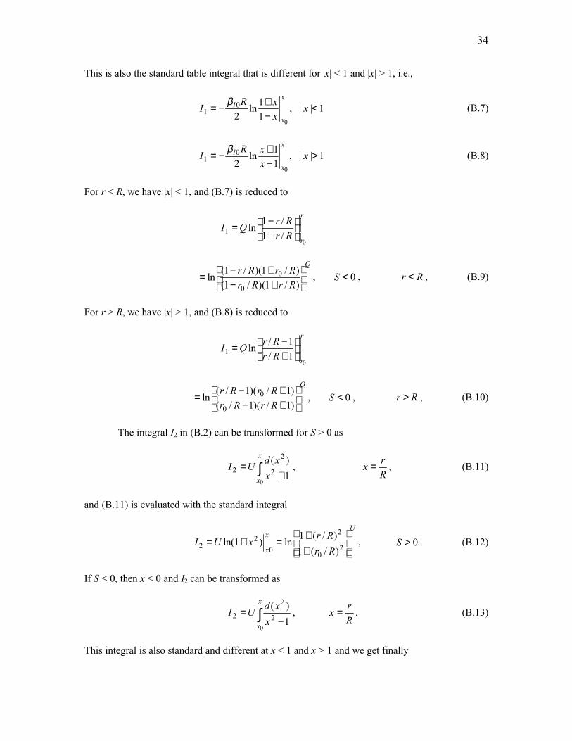
This is also the standard table integral that is different for |x| < 1 and |x| > 1, i.e.,
1||,11ln
20
01 <
−+
−= xxxRI
x
x
lβ (B.7)
1||,11ln
20
01 >
−+
−= xxxRI
x
x
lβ (B.8)
For r < R, we have |x| < 1, and (B.7) is reduced to
r
rRrRrQI
0/1/1ln1
+−
=
Q
RrRrRrRr
+−
+−=
)/1)(/1()/1)(/1(ln
0
0 , 0<S , Rr < , (B.9)
For r > R, we have |x| > 1, and (B.8) is reduced to
r
rRrRrQI
01/1/ln1
+−
=
Q
RrRrRrRr
+−+−
=)1/)(1/()1/)(1/(ln
0
0 , 0<S , Rr > , (B.10)
The integral I2 in (B.2) can be transformed for S > 0 as
∫ +=
x
x xxdUI
01)(
2
2
2 ,Rrx = , (B.11)
and (B.11) is evaluated with the standard integral
Ux
x RrRrxUI
++
=+= 20
2
02
2 )/(1)/(1ln)1ln( , 0>S . (B.12)
If S < 0, then x < 0 and I2 can be transformed as
∫ −=
x
x xxdUI
01)(
2
2
2 ,Rrx = . (B.13)
This integral is also standard and different at x < 1 and x > 1 and we get finally

35
U
RrRrI
−−
= 20
2
2 )/(1)/(1ln , ,0<S and Rr < , (B.14)
U
RrRrI
+−
=1)/(1)/(ln 2
0
2
2 , ,0<S and Rr > . (B.15)
These expressions for I1 and I2 are used in section 3.2 for the large-size fraction.
Appendix C
Evaluation of the integrals in section 3.3 for v(r) = Avr1/2
If v(r) = Avr1/2, then Bv = 1/2 and I1, I2 in section 3.3can be rewritten for S > 0 as
1101 HII lβ−= , ∫ +=
2
12/311 1
r
r tdtI (C.1)
212 2IVI = , ∫ +
=2
12/321 1
r
r ttdtI (C.2)
where
Hrt = ,
3/2||
=
vAsbH
χ,
v
llA
HkwVχαα 2/1)(2 −
= . (C.3)
Here the dimensions in CGS units are [Av] = cm1/2 s-1, [H] = cm, V is dimensionless. Introducing a
new variable x = t1/2, the integral I11 can be transformed into that given in Gradshteyn and Ryzhik
(1994, hereafter GR94):
∫∫ +=
+=
x
x
t
t xxdx
tdtI
0032/311 1
21
x
x
xx
xx
03
12arctan3
1)1(
1ln612 2
2
−++
+−−= . (C.4)
Then finally

36
−−
−−
+−+
+−+=
312arctan
312arctan
31
)1()1()1()1(ln2 0
6/1
220
200
2
01xx
xxxxxxHI lβ . (C.5)
Here and in subsequent equations, x = (r/H)1/2.
The integral I21 in (C.2) can be evaluated with the same substitution, x = t1/2,
∫∫ +=
+=
x
x
t
t xdxx
ttdtI
003
3
2/321 12
1
x
xx
xxxxx
02
3arctan3
1)1(
1ln312 2/12
−−
+−+−= . (C.6)
The last integral is from GR94. Substitution into (C.2) yields
−−
−−
+−+
+−+−=
0
03/1
2/120
2/1200
2 23arctan
23arctan
31
)1)(1()1)(1(ln
xx
xx
xxxxxxxVI , (C.7)
For S < 0, I1 can be transformed as
1201 HII lβ−= , ∫ −=
t
t tdtI
02/312 1
(C.8)
With the same substitution, x = t1/2, the integral I12 can be reduced to that given in GR94
∫∫ −=
−=
x
x
t
t xxdx
tdtI
0032/312 1
21
x
x
xxx
x
03
12arctan3
11
)1(ln612 2
2
++++
−−= (C.9)
Then finally
+−
+−
++−
++−=
312arctan
312arctan
31
)1()1()1()1(ln2 0
6/1
220
200
2
01xx
xxxxxxHI lβ . (C.10)
For S < 0, I2 can be transformed as

37
222 2IVI −= , ∫ −
=t
t ttdtI
02/322 1
(C.11)
With the same substitution, x = t1/2, it can be transformed to the form given in GR94
∫ −=
x
x xdxxI
03
3
22 12
x
xx
xxxxx
02
3arctan3
11
)1(ln312
2/12
++
−+++−= . (C.12)
Substitution into (C.11) yields:
+−
+−
−++
−++−=
0
03/1
2/1200
02/12
2 23arctan
23arctan
31
)1()1()1()1(ln
xx
xx
xxxxxxxVI . (C.13)
These 4 integrals are used in section 3.3 for evaluation of the size spectra fl for v(r) = Avr1/2.

38
References
Böhm, J. P., 1989: A general equation for the terminal fall speed of solid hydrometeors. J. Atmos.
Sci., 46, 2419-2427.
Brandes, E. A., G. Zhang, and J. Vivekanandan, 2003: An evaluation of a drop distribution-based
polarimetric radar rainfall estimator. J. Appl. Meteor., 42, 652–660.
Brown, P. S., 1991: Parameterization of the evolving drop-size distribution based on analytic
solution of the linearized coalescence breakup equation. J. Atmos. Sci., 48, 200-210.
——, 1997: Mass conservation considerations in analytic representation of rain drop fragment
distribution. J. Atmos. Sci., 54, 1675–1687.
Cotton, W. R., R. A. Anthes, 1989: Storm and Cloud Dynamics, Academic Press, 883 pp.
Golovin, A. M., 1963: On the kinetic equation for coagulating cloud droplets with allowance for
condensation. Izv. Acad. Sci. USSR, Ser. Geophys., 10, 949-953.
Feingold, G., S. Tzivion, and Z. Levin, 1988: Evolution of raindrop spectra. Part I: Solution to the
collection/breakup equation using the method of moments. J. Atmos. Sci., 45, 3387–3399.
Gunn, K. L. S., and Marshall, J. S., 1958: The distribution with size of aggregates snowflakes. J.
Meteorol., 15, 452-461.
Gradshteyn, I. S. and I. M. Ryzhik, 1994: Table of Integrals, Series, and Products, 5th ed., A.
Jeffery, Ed., Academic Press, 1204 pp.
Heymsfield, A. J., 2003: Properties of tropical and midlatitude ice cloud particle ensembles. Part
II: Application for mesoscale and climate models. J. Atmos. Sci., 60, 2592-2611.
Heymsfield, A. J. and C. M. R. Platt, 1984: A parameterization of the particle size spectrum of ice
clouds in terms of the ambient temperature and the ice water content. J. Atmos. Sci., 41,
846-855.
Houze, R. A., P. V. Hobbs, P. H. Herzegh, and D. B. Parsons, 1979: Size distribution of
precipitating particles in frontal clouds. J. Atmos. Sci., 36, 156-162.

39
Hu, Z., and R. C. Srivastava, 1995: Evolution of raindrop size distribution by coalescence,
breakup, and evaporation: Theory and observations. J. Atmos. Sci., 52, 1761–1783.
Joss, J., and E. G. Gori, 1978: Shapes of raindrop size distributions. J. Appl. Meteorol, 17, 1054-
1061.
Kessler, E., 1969: On the distribution and continuity of water substance in atmospheric
circulation. Meteorol. Monogr., 10, No.32, Amer. Meteor. Soc., 84 pp.
Khvorostyanov, V. I., and J. A. Curry, 1999a: Toward the theory of stochastic condensation in
clouds. Part I: A general kinetic equation. J. Atmos. Sci., 56, 3985-3996.
——, and ——, 1999b: Toward the theory of stochastic condensation in clouds. Part II.
Analytical solutions of gamma distribution type. J. Atmos. Sci., 56, 3997-4013.
——, and ——, 2002: Terminal velocities of droplets and crystals: power laws with continuous
parameters over the size spectrum. J. Atmos. Sci., 59, 1872-1884.
——, and ——, 2005. Fall velocities of hydrometeors in the atmosphere: Refinements to a
continuous analytical power law. J. Atmos. Sci., 62, 4343–4357.
——, and ——, 2008: Analytical solutions to the stochastic kinetic equation for liquid and ice
particle size spectra in precipitating and non-precipitating clouds. Part I: small-size fraction.
J. Atmos. Sci., 65, in press (this issue)
——, and K. Sassen, 2002: Microphysical processes in cirrus and their impact on radiation, a
mesoscale modeling perspective, in “Cirrus”, Oxford University Press, Eds. D. Lynch, K.
Sassen, D. Starr and G. Stephens, 397-432.
——, J. A. Curry, J. O. Pinto, M. Shupe, B. A. Baker, and K. Sassen, 2001: Modeling with
explicit spectral water and ice microphysics of a two-layer cloud system of altostratus and
cirrus observed during the FIRE Arctic Clouds Experiment. J. Geophys. Res., 106, 15,099-
15,112.

40
Liu, Y., 1993: Statistical theory of the Marshall-Palmer distribution of raindrops. Atmos.
Environ., 27A, 15-19.
Low, T. B., and R. List, 1982a: Collision, coalescence, and breakup of raindrops. Part I:
Experimentally established coalescence efficiencies and fragment size distributions in
breakup. J. Atmos. Sci., 39, 1591–1606.
——, and ——, 1982b: Collision, coalescence, and breakup of raindrops. Part II:
Parameterization of fragment size distributions. J. Atmos. Sci., 39, 1607–1618.
Marshall, J. S., and W. M. K. Palmer, 1948: The distribution of raindrops with size. J. Meteor., 5,
165–166.
McFarquhar, G. M., 2004: A new representation of collision-induced breakup of raindrops and its
implications for the shapes of raindrop size distributions. J. Atmos. Sci., 61, 777-794.
Mitchell, D. L., 1994: A model predicting the evolution of ice particle size spectra and radiative
properties of cirrus clouds. Part I: Microphysics. J. Atmos. Sci., 51, 797-816.
______, 1996: Use of mass- and area-dimensional power laws for determining precipitation
particle terminal velocities. J. Atmos. Sci., 53, 1710-1723.
______, S. K. Chai, Y. Liu, A. J. Heymsfield and Y. Dong, 1996: Modeling cirrus clouds. Part I:
Treatment of bimodal spectra and case study analysis. J. Atmos. Sci., 53, 2952-2966.
Passarelli, R. E., 1978a: An approximate analytical model of the vapor deposition and
aggregation growth of snowflakes. J. Atmos. Sci., 35, 118-124.
______, 1978b: Theoretical and observational study of snow-sized spectra and snowflake
aggregation efficiencies. J. Atmos. Sci., 35, 882-889.
Platt, C. M. R., 1997: A parameterization of the visible extinction coefficient in terms of the
ice/water content. J. Atmos. Sci., 54, 2083-2098.
Pruppacher, H. R., and Klett, J. D., 1997: Microphysics of Clouds and Precipitation, 2nd Edition,
Kluwer, 997 pp.
Rogers, R. R, 1979: A Short Course in Cloud Physics. 2nd ed., Pergamon Press, 235 pp.

41
Ryan, B. F, 2000: A bulk parameterization of the ice particles size distribution and the optical
properties in ice clouds. J. Atmos. Sci., 57, 1436-1451.
Sassen, K., D. O’C. Starr, and T. Uttal, 1989: Mesoscale and microscale structure of cirrus
clouds: Three case studies. J. Atmos. Sci., 46, 371-396.
Scott, W. T., 1968: Analytic studies of cloud droplet coalescence. J. Atmos. Sci., 25, 54-65.
Seifert, A., 2005: On the shape-slope relation of drop size distributions in convective rain. J.
Appl. Meteorol. 44, 1146-1151.
Srivastava, R., C., 1971: Size distribution of raindrops generated by their breakup and
coalescence. J. Atmos. Sci., 28, 410- 415.
——, 1978: Parameterization of raindrop size distribution. J. Atmos. Sci., 35, 108 - 117.
——, 1982: A simple model of particle coalescence and breakup. J. Atmos. Sci., 39, 1317 - 1322.
______, and R. E. Passarelli, 1980: Analytical solutions to simple models of condensation and
coalescence. J. Atmos. Sci., 37, 612-621.
Ulbrich, C. W., 1983: Natural variations in the analytical form of the raindrop size distribution. J.
Climate Appl. Meteor., 22, 1764–1775.
Verlinde, J., P. J. Flatau, and W. R. Cotton, 1990: Analytical solutions to the collection growth
equation: comparison with approximate methods and application to cloud microphysics
parameterization schemes. J. Atmos. Sci., 47, 2871-2880.
Voloshchuk, V. M., 1984: The Kinetic Theory of Coagulation. Hydrometeoizdat, Leningrad, 283
pp.
Willis, P. T., 1984: Functional fits to some observed drop size distributions and parameterization
of rain. J. Atmos. Sci., 41, 1648-1661.
Zawadski, I., and de M. A. de Agostinho, 1988: Equilibrium raindrop size distributions in tropical
rain. J. Atmos. Sci., 45, 3452 - 3459.

42
Zhang, G., J. Vivekanandan, and E. A. Brandes, 2001: A method for estimating rain rate and drop
size distribution from polarimetric radar measurements. IEEE Trans. Geosci. Remote Sens.,
39, 830-841.
——, ——, and E. A. Brandes, 2003a: Constrained gamma drop size distribution model for
polarimetric radar rain estimation: Justification and development. Preprints, 31st Int. Conf.
on Radar Meteorology, Seattle, WA, Amer. Meteor. Soc., 206-225.
——, ——, ——, R. Meneghini, and T. Kozu, 2003b: The shape- slope relation in observed
gamma raindrop size distributions: Statistical error or useful information? J. Atmos.
Oceanic Technol., 20, 1106-1119.

43
Figure captions
Fig. 1. Profiles for calculations of the spectra of the large fraction: (a) IWC of the large fraction
(solid circles), and of the small fraction in the baseline case (open circles) and with doubled IWC
(open diamonds); (b) parameter αl; (c) ice supersaturation.
Fig. 2. (a) Exponential slope βl0 and (b) Λl0 of the size spectra of the large-size fraction calculated
with the IWC of small-size fraction qls (circles) and 2qls (diamonds) as described in Part 1. The
generalized experimental slope for crystalline clouds from Platt (1997) and Ryan (2000)
recalculated from the temperature to height with the average lapse rate 6.5 ºK km-1 is plotted in
(b) with triangles.
Figure 3. Crystal size spectra by radii r (L-1 µm-1) at ice subsaturation at the heights in km
indicated in the legends and the temperatures decreasing from -14.9 ºC at 4.8 km to -22.15 ºC at
6.0 km. (a) small fraction; (b) large fraction; (c) composite; (d) generalization by Platt (1997) of
the observed crystal size spectra by long dimension D (m-4) in the temperature interval -25 ºC to -
30 ºC. Note different normalization of the spectra and axes scales in (a)-(c) by radius and (d) by
diameter.
Fig. 4. Crystal size spectra by radii (L-1 µm-1) at ice supersaturation at the heights indicated in the
legends. (a) for the small fraction extended to 200 µm; (b) for the large fraction; (c) composite
spectra; and (d) experimental spectra in cirrus clouds from Lawson et al. (2006) at 3 indicated
temperatures.
Fig. 5. (a) Slopes and (b) size spectra in the subcloud layer with zero IWC of small-size fraction
qls at the heights (km) indicated in the legends.

0.00 0.05 0.10 0.15IWC (g m-3)
3
4
5
6
7
8
9
10
11
12H
eigh
t(km
)(a)
-1.0 -0.5 0.0 0.5αl (km-1)
3
4
5
6
7
8
9
10
11
12
Hei
ght(
km)
(b)
-80 -70 -60 -50 -40 -30 -20 -10 0 10 20Ice supersaturation (%)
3
4
5
6
7
8
9
10
11
12
Hei
ght(
km)
(c)

0 100 200 300 400 500β0,l (cm-1)
3
4
5
6
7
8
9H
eigh
t(km
)(a)
1
2
0 50 100 150 200 250Λ0,l (cm-1)
3
4
5
6
7
8
9
Hei
ght(
km)
(b)
1
2

1 10 100Crystal radius (µm)
1E-3
1E-2
1E-1
1E+0
1E+1
1E+2C
ryst
alsi
zesp
ectra
(L-1
µm-1
)(a)
4.8 km
5.1 km
5.4 km
5.7 km
6.0 km
1 10 100 1000Crystal radius (µm)
1E-7
1E-6
1E-5
1E-4
1E-3
1E-2
1E-1
1E+0
1E+1
1E+2
1E+3
Cry
stal
size
spec
tra(L
-1µm
-1)
(c)
4.8
5.1
5.4
5.7
6.0
0 500 1000 1500 2000 2500Crystal radius (µm)
1E-7
1E-6
1E-5
1E-4
1E-3
1E-2
1E-1
1E+0
Cry
stal
size
spec
tra(L
-1µm
-1)
(b) 4.8 km
5.1 km
5.4 km
5.7 km
6.0 km
1 10 100 1000Long dimension D (µm)
1E+3
1E+4
1E+5
1E+6
1E+7
1E+8
1E+9
1E+10
1E+11
1E+12
Crys
tals
ize
spec
tra
f(D
)m
-4(d)

1 10 100Crystal radius (µm)
1E-4
1E-3
1E-2
1E-1
1E+0
1E+1
1E+2C
ryst
alsi
zesp
ectra
(L-1
µm-1
)(a)
7.5 km
7.8 km
8.1 km
8.4 km
8.7 km
1 10 100 1000Crystal radius (µm)
1E-6
1E-5
1E-4
1E-3
1E-2
1E-1
1E+0
1E+1
1E+2
Cry
stal
size
spec
tra(L
-1µm
-1)
(c)
7.5 km
7.8 km
8.1 km
8.4 km
0 200 400 600 800 1000Crystal radius (µm)
1E-7
1E-6
1E-5
1E-4
1E-3
1E-2
1E-1
1E+0
1E+1
Cry
stal
size
spec
tra(L
-1µm
-1)
(b)7.5 km
7.8 km
8.1 km
8.4 km
1 10 100 1000Maximum dimension D (µm)
1E-6
1E-5
1E-4
1E-3
1E-2
1E-1
1E+0
1E+1
1E+2
1E+3
Crys
tals
ize
spec
tra
(L-1
µm-1
)-54.8 C
-45.2 C
-35.7 C
(d)

0 200 400 600 800Crystal radius (µm)
1E+1
1E+2
1E+3
1E+4S
lope
(cm
-2)
(a)
3.3 km
3.6 km
3.9 km
0 200 400 600 800Crystal radius (µm)
1E-4
1E-3
1E-2
1E-1
1E+0
1E+1
1E+2
Cry
stal
size
spec
tra(L
-1µ m
-1)
(b)3.3 km
3.6 km
3.9 km