analytical modelling of wells with in ow control devices
TRANSCRIPT
Analytical Modelling of Wellswith Inflow Control Devices
Vasily Mihailovich Birchenko
Submitted for the degree of
Doctor of Philosophy
Institute of Petroleum Engineering
Heriot-Watt University
July 2010
The copyright in this thesis is owned by the author. Any quotation from
the thesis or use of any of the information contained in it must acknowledge
this thesis as the source of the quotation or information.

Abstract
Inflow Control Devices (ICD) have been successfully used in hundreds of wells
around the world during the last decade and are now considered to be a mature
well completion technology. This work is dedicated to the methodology of making
following three decisions with respect to ICD application:
1. Selection between ICD and Interval Control Valves (ICV), the other advanced
completion technology.
2. Identification of whether particular well is likely to benefit from ICD.
3. Quantification of the anticipated positive effect.
Design of an advanced completion for a particular field application often includes
feasibility studies on both ICV and ICD. The choice between these two technolo-
gies is not always obvious and the need for general methodology on making this
choice is recognised by the petroleum industry. In this dissertation ICD has been
compared against the competing ICV technology with particular emphasis on issues
such as uncertainty in the reservoir description, inflow performance and formation
permeability. The methodology of selection between ICD and ICV is proposed.
The benefits of ICD application can, by and large, be attributed to reduction of
the following two effects detrimental to horizontal well performance:
• Inflow profile skewing by frictional pressure loss along the completion (heel-toe
effect).
• Inflow variation caused by reservoir heterogeneity.
Frictional pressure drop along the completion is an important design factor for
horizontal wells. It has to be taken into account in order to secure optimum reser-
voir drainage and avoid overestimation of well productivity. Many authors have

previously addressed various aspects of this problem, but an explicit analytical so-
lution for turbulent flow in wellbore has not so far been published. This dissertation
presents such a solution based on the same assumptions as those of previous re-
searchers.
New method to quantify the reduction of inflow imbalance caused by the fric-
tional pressure loss along a horizontal completion is proposed. The equation de-
scribing this phenomenon in homogeneous reservoir is derived and two solutions pre-
sented: an analytical approximation and a more precise numerical solution. Mathe-
matical model for effective reduction of the inflow imbalance caused by the reservoir
heterogeneity is also presented.
The trade-off between well productivity and inflow equalisation is a key engi-
neering issue when applying ICD technology. Presented solutions quantitatively
addresses this issue. Their practical utility is illustrated through case studies.
ii

To those who fought against the Nazis in 1939-1945.

Acknowledgements
I would like to express deep gratitude to my supervisor, Professor David R.
Davies, for sharing with me his wide spectrum of petroleum engineering experience.
His guidance, understanding, patience and meticulous remarks helped me very much
throughout the course of this research.
I am thankful to the sponsors of the “Added Value from Intelligent Field & Well
system Technology” JIP at Heriot-Watt University for the financial support and
feedback on my work. I am especially grateful to Mike R. Konopczynski (Hallibur-
ton) who initiated the “ICV versus ICD” comparison project and advised me during
its course.
I would like to thank my colleague Faisal T. Al-Khelaiwi for our fruitful discus-
sions on advanced well completions and his help with the literature review on this
subject.
With regards to the uncertainty chapter of this thesis I thank Dr. Vasily V. De-
myanov, Dr. Jerome Vidal and Ivan Grebenkin. Vasily has kindly advised me on
Geostatistics and Uncertainty Quantification methods. Jerome particularly appre-
ciated this chapter from the reservoir engineering viewpoint and gave a number of
valuable recommendations on its possible extension. My colleague Ivan continues
research in this direction. He has verified my results at the introductory stage of his
own work.
I would like to extend my gratitude to Dr. Alexandr V. Usnich (University of
Zurich) and Dr. Andrei Iu. Bejan (University of Cambridge) who consulted me on
certain mathematical aspects of this dissertation. Alexandr advised me on properties
of the Weierstrass elliptic function. Discussion of Chapter 6 with Andrei have helped
me to formulate my ideas more rigorously and succinctly. He also kindly checked
the derivation of formulae presented in that chapter.

I am indebted to my colleague Khafiz Muradov who has helped me to find ap-
proximate analytical solution presented in Chapter 5.
I thank AGR Group, Schlumberger and Weatherford for providing access to their
software.
Last, but not the least, I would like to acknowledge the organisations primarily
responsible for the education I received prior to beginning of this research: Lyceum
of Belarusian State University, Moscow Institute of Physics and Technology, Yukos
oil company.
v
Table of Contents
List of Tables x
List of Figures xii
Nomenclature xv
List of Publications xxi
1 Introduction 1
1.1 Well-Reservoir Contact . . . . . . . . . . . . . . . . . . . . . . . . . . 1
1.2 Advanced Well Completions . . . . . . . . . . . . . . . . . . . . . . . 2
1.3 The Scope of This Dissertation . . . . . . . . . . . . . . . . . . . . . 5
2 How to Make the Choice between Passive and Active Inflow-Control
Completions 8
2.1 Introduction . . . . . . . . . . . . . . . . . . . . . . . . . . . . . . . . 8
2.2 Uncertainty in the Reservoir Description . . . . . . . . . . . . . . . . 9
2.3 More Flexible Development . . . . . . . . . . . . . . . . . . . . . . . 11
2.3.1 Reactive Control Based on “Unwanted” Fluid Flows . . . . . . 11
2.3.2 Proactive Control . . . . . . . . . . . . . . . . . . . . . . . . . 11
2.3.3 Real Time Optimization . . . . . . . . . . . . . . . . . . . . . 12
2.4 Number of Controllable Zones . . . . . . . . . . . . . . . . . . . . . . 12
2.5 Inner Flow Conduit Diameter . . . . . . . . . . . . . . . . . . . . . . 13
2.5.1 Completion Sizes . . . . . . . . . . . . . . . . . . . . . . . . . 13
2.5.2 Impact of the Inner Flow Conduit Diameter on Inflow Perfor-
mance . . . . . . . . . . . . . . . . . . . . . . . . . . . . . . . 15
vi

Table of Contents
2.5.3 Inflow Distribution along the Wellbore . . . . . . . . . . . . . 17
2.5.4 Inflow Performance Relationship . . . . . . . . . . . . . . . . . 20
2.6 Formation Permeability . . . . . . . . . . . . . . . . . . . . . . . . . . 21
2.7 Value of Information . . . . . . . . . . . . . . . . . . . . . . . . . . . 24
2.8 Multilateral Wells . . . . . . . . . . . . . . . . . . . . . . . . . . . . . 25
2.9 Multiple Reservoir Management (MRM) . . . . . . . . . . . . . . . . 26
2.10 Long Term Equipment Reliability . . . . . . . . . . . . . . . . . . . . 27
2.11 Reservoir Isolation Barrier . . . . . . . . . . . . . . . . . . . . . . . . 29
2.12 Improved Well Clean-Up . . . . . . . . . . . . . . . . . . . . . . . . . 30
2.13 Bullhead Selective Acidizing or Scale Treatment . . . . . . . . . . . . 30
2.14 Equipment Cost . . . . . . . . . . . . . . . . . . . . . . . . . . . . . . 31
2.15 Installation . . . . . . . . . . . . . . . . . . . . . . . . . . . . . . . . 31
2.16 Gas Fields . . . . . . . . . . . . . . . . . . . . . . . . . . . . . . . . . 31
2.16.1 Retrograde Condensate Gas . . . . . . . . . . . . . . . . . . . 32
2.16.2 Dry Gas . . . . . . . . . . . . . . . . . . . . . . . . . . . . . . 32
2.16.3 Wet Gas . . . . . . . . . . . . . . . . . . . . . . . . . . . . . . 33
2.17 Conclusions . . . . . . . . . . . . . . . . . . . . . . . . . . . . . . . . 33
3 Impact of Reservoir Uncertainty on Selection of Advanced Com-
pletion Type 34
3.1 Introduction . . . . . . . . . . . . . . . . . . . . . . . . . . . . . . . . 34
3.2 Literature Review . . . . . . . . . . . . . . . . . . . . . . . . . . . . . 38
3.3 Advanced Well Completions . . . . . . . . . . . . . . . . . . . . . . . 39
3.4 Choice of Reservoir Model . . . . . . . . . . . . . . . . . . . . . . . . 41
3.5 The Base Case . . . . . . . . . . . . . . . . . . . . . . . . . . . . . . 42
3.6 Advanced Completion Cases . . . . . . . . . . . . . . . . . . . . . . . 44
3.6.1 ICD Case . . . . . . . . . . . . . . . . . . . . . . . . . . . . . 44
3.6.2 ICV Case . . . . . . . . . . . . . . . . . . . . . . . . . . . . . 46
3.7 Results . . . . . . . . . . . . . . . . . . . . . . . . . . . . . . . . . . . 47
3.8 Discussion . . . . . . . . . . . . . . . . . . . . . . . . . . . . . . . . . 49
3.9 Conclusions . . . . . . . . . . . . . . . . . . . . . . . . . . . . . . . . 50
vii
Table of Contents
4 Impact of Frictional Pressure Losses Along the Completion on Well
Performance 51
4.1 Introduction . . . . . . . . . . . . . . . . . . . . . . . . . . . . . . . . 51
4.2 Literature Review . . . . . . . . . . . . . . . . . . . . . . . . . . . . . 52
4.3 Problem Formulation . . . . . . . . . . . . . . . . . . . . . . . . . . . 55
4.3.1 Assumptions . . . . . . . . . . . . . . . . . . . . . . . . . . . . 55
4.3.2 Mathematical Formulation . . . . . . . . . . . . . . . . . . . . 58
4.4 Derivation of the Solution . . . . . . . . . . . . . . . . . . . . . . . . 60
4.4.1 General Solution . . . . . . . . . . . . . . . . . . . . . . . . . 60
4.4.2 Boundary Value Problem of Rate Constrained Well . . . . . . 64
4.4.3 Boundary Value Problem of Pressure Constrained Well . . . . 65
4.5 The Solution for Frictional Pressure Losses Along the Completion . . 67
4.5.1 Rate Constrained Well . . . . . . . . . . . . . . . . . . . . . . 67
4.5.2 Pressure Constrained Well . . . . . . . . . . . . . . . . . . . . 69
4.6 Model Verification . . . . . . . . . . . . . . . . . . . . . . . . . . . . 71
4.6.1 Seines et al. (1993) . . . . . . . . . . . . . . . . . . . . . . . . 71
4.6.2 Halvorsen (1994) . . . . . . . . . . . . . . . . . . . . . . . . . 73
4.6.3 Penmatcha et al. (1999) . . . . . . . . . . . . . . . . . . . . . 73
4.6.4 Numerical Simulation . . . . . . . . . . . . . . . . . . . . . . . 74
4.7 Discussion . . . . . . . . . . . . . . . . . . . . . . . . . . . . . . . . . 75
4.8 Conclusions . . . . . . . . . . . . . . . . . . . . . . . . . . . . . . . . 76
5 Reduction of the Horizontal Well’s Heel-Toe Effect with Inflow
Control Devices 78
5.1 Introduction . . . . . . . . . . . . . . . . . . . . . . . . . . . . . . . . 78
5.2 Assumptions . . . . . . . . . . . . . . . . . . . . . . . . . . . . . . . . 80
5.3 Problem Formulation . . . . . . . . . . . . . . . . . . . . . . . . . . . 82
5.3.1 General Formulation . . . . . . . . . . . . . . . . . . . . . . . 82
5.3.2 Formulation for a Homogeneous Reservoir . . . . . . . . . . . 84
5.4 Solution . . . . . . . . . . . . . . . . . . . . . . . . . . . . . . . . . . 85
5.4.1 Qualitative Analysis . . . . . . . . . . . . . . . . . . . . . . . 85
viii
Table of Contents
5.4.2 Approximate Analytical Solution . . . . . . . . . . . . . . . . 86
5.4.3 Numerical Solution . . . . . . . . . . . . . . . . . . . . . . . . 88
5.5 Choosing an Appropriate ICD Strength . . . . . . . . . . . . . . . . . 88
5.6 Case Study . . . . . . . . . . . . . . . . . . . . . . . . . . . . . . . . 90
5.7 Discussion . . . . . . . . . . . . . . . . . . . . . . . . . . . . . . . . . 94
5.8 Conclusions . . . . . . . . . . . . . . . . . . . . . . . . . . . . . . . . 95
6 Application of Inflow Control Devices to Heterogeneous Reservoirs 97
6.1 Introduction . . . . . . . . . . . . . . . . . . . . . . . . . . . . . . . . 97
6.2 Assumptions . . . . . . . . . . . . . . . . . . . . . . . . . . . . . . . . 97
6.3 Problem Formulation . . . . . . . . . . . . . . . . . . . . . . . . . . . 99
6.4 Solution . . . . . . . . . . . . . . . . . . . . . . . . . . . . . . . . . . 100
6.4.1 Uniform Distribution of Specific Productivity Index . . . . . . 101
6.4.2 Triangular Distribution of Specific Productivity Index . . . . . 102
6.5 Case Study . . . . . . . . . . . . . . . . . . . . . . . . . . . . . . . . 103
6.5.1 Highly Productive Reservoir . . . . . . . . . . . . . . . . . . . 104
6.5.2 Medium Productivity Reservoir . . . . . . . . . . . . . . . . . 105
6.6 Discussion . . . . . . . . . . . . . . . . . . . . . . . . . . . . . . . . . 107
6.7 Conclusions . . . . . . . . . . . . . . . . . . . . . . . . . . . . . . . . 109
7 Conclusions and Future Work 110
7.1 Conclusions . . . . . . . . . . . . . . . . . . . . . . . . . . . . . . . . 110
7.2 Future Work . . . . . . . . . . . . . . . . . . . . . . . . . . . . . . . . 112
Bibliography 112
A Friction Factor Calculation 125
B Pressure Drop due to Acceleration 129
C The Upper Estimate of Frictional Pressure Drop 131
D Comparison to Halvorsen’s Solution 133
ix
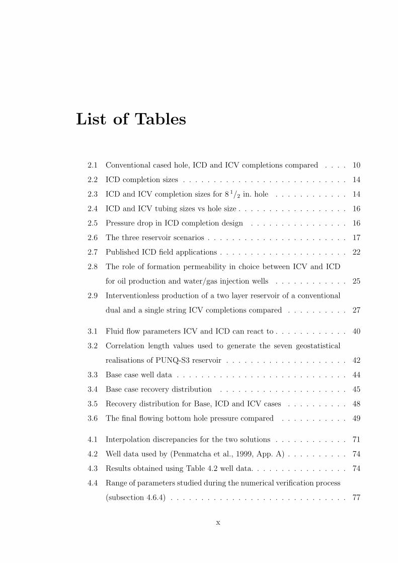
List of Tables
2.1 Conventional cased hole, ICD and ICV completions compared . . . . 10
2.2 ICD completion sizes . . . . . . . . . . . . . . . . . . . . . . . . . . . 14
2.3 ICD and ICV completion sizes for 8 1/2 in. hole . . . . . . . . . . . . 14
2.4 ICD and ICV tubing sizes vs hole size . . . . . . . . . . . . . . . . . . 16
2.5 Pressure drop in ICD completion design . . . . . . . . . . . . . . . . 16
2.6 The three reservoir scenarios . . . . . . . . . . . . . . . . . . . . . . . 17
2.7 Published ICD field applications . . . . . . . . . . . . . . . . . . . . . 22
2.8 The role of formation permeability in choice between ICV and ICD
for oil production and water/gas injection wells . . . . . . . . . . . . 25
2.9 Interventionless production of a two layer reservoir of a conventional
dual and a single string ICV completions compared . . . . . . . . . . 27
3.1 Fluid flow parameters ICV and ICD can react to . . . . . . . . . . . . 40
3.2 Correlation length values used to generate the seven geostatistical
realisations of PUNQ-S3 reservoir . . . . . . . . . . . . . . . . . . . . 42
3.3 Base case well data . . . . . . . . . . . . . . . . . . . . . . . . . . . . 44
3.4 Base case recovery distribution . . . . . . . . . . . . . . . . . . . . . 45
3.5 Recovery distribution for Base, ICD and ICV cases . . . . . . . . . . 48
3.6 The final flowing bottom hole pressure compared . . . . . . . . . . . 49
4.1 Interpolation discrepancies for the two solutions . . . . . . . . . . . . 71
4.2 Well data used by (Penmatcha et al., 1999, App. A) . . . . . . . . . . 74
4.3 Results obtained using Table 4.2 well data. . . . . . . . . . . . . . . . 74
4.4 Range of parameters studied during the numerical verification process
(subsection 4.6.4) . . . . . . . . . . . . . . . . . . . . . . . . . . . . . 77
x

List of Tables
4.5 Pressure mismatch with numerical simulation . . . . . . . . . . . . . 77
5.1 Channel ICD strength . . . . . . . . . . . . . . . . . . . . . . . . . . 83
5.2 Typical Troll oil well data . . . . . . . . . . . . . . . . . . . . . . . . 91
6.1 Highly productive reservoir case study data . . . . . . . . . . . . . . . 104
6.2 Medium productivity reservoir case study . . . . . . . . . . . . . . . . 106
xi
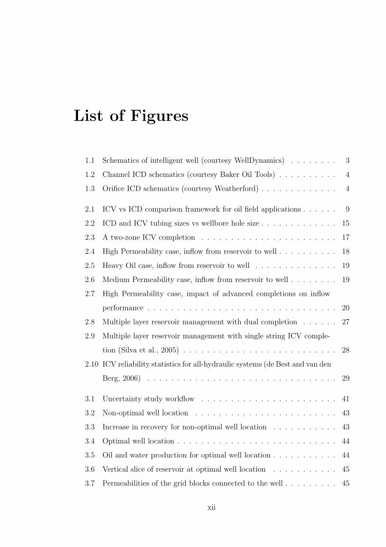
List of Figures
1.1 Schematics of intelligent well (courtesy WellDynamics) . . . . . . . . 3
1.2 Channel ICD schematics (courtesy Baker Oil Tools) . . . . . . . . . . 4
1.3 Orifice ICD schematics (courtesy Weatherford) . . . . . . . . . . . . . 4
2.1 ICV vs ICD comparison framework for oil field applications . . . . . . 9
2.2 ICD and ICV tubing sizes vs wellbore hole size . . . . . . . . . . . . . 15
2.3 A two-zone ICV completion . . . . . . . . . . . . . . . . . . . . . . . 17
2.4 High Permeability case, inflow from reservoir to well . . . . . . . . . . 18
2.5 Heavy Oil case, inflow from reservoir to well . . . . . . . . . . . . . . 19
2.6 Medium Permeability case, inflow from reservoir to well . . . . . . . . 19
2.7 High Permeability case, impact of advanced completions on inflow
performance . . . . . . . . . . . . . . . . . . . . . . . . . . . . . . . . 20
2.8 Multiple layer reservoir management with dual completion . . . . . . 27
2.9 Multiple layer reservoir management with single string ICV comple-
tion (Silva et al., 2005) . . . . . . . . . . . . . . . . . . . . . . . . . . 28
2.10 ICV reliability statistics for all-hydraulic systems (de Best and van den
Berg, 2006) . . . . . . . . . . . . . . . . . . . . . . . . . . . . . . . . 29
3.1 Uncertainty study workflow . . . . . . . . . . . . . . . . . . . . . . . 41
3.2 Non-optimal well location . . . . . . . . . . . . . . . . . . . . . . . . 43
3.3 Increase in recovery for non-optimal well location . . . . . . . . . . . 43
3.4 Optimal well location . . . . . . . . . . . . . . . . . . . . . . . . . . . 44
3.5 Oil and water production for optimal well location . . . . . . . . . . . 44
3.6 Vertical slice of reservoir at optimal well location . . . . . . . . . . . 45
3.7 Permeabilities of the grid blocks connected to the well . . . . . . . . . 45
xii
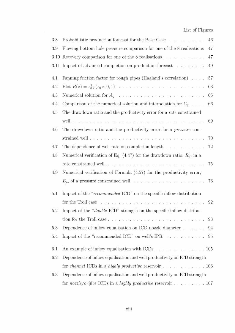
List of Figures
3.8 Probabilistic production forecast for the Base Case . . . . . . . . . . 46
3.9 Flowing bottom hole pressure comparison for one of the 8 realisations 47
3.10 Recovery comparison for one of the 8 realisations . . . . . . . . . . . 47
3.11 Impact of advanced completion on production forecast . . . . . . . . 49
4.1 Fanning friction factor for rough pipes (Haaland’s correlation) . . . . 57
4.2 Plot R(z) = z20℘(z0 z; 0, 1) . . . . . . . . . . . . . . . . . . . . . . . . 63
4.3 Numerical solution for Aq . . . . . . . . . . . . . . . . . . . . . . . . 65
4.4 Comparison of the numerical solution and interpolation for Cq . . . . 66
4.5 The drawdown ratio and the productivity error for a rate constrained
well . . . . . . . . . . . . . . . . . . . . . . . . . . . . . . . . . . . . . 69
4.6 The drawdown ratio and the productivity error for a pressure con-
strained well . . . . . . . . . . . . . . . . . . . . . . . . . . . . . . . . 70
4.7 The dependence of well rate on completion length . . . . . . . . . . . 72
4.8 Numerical verification of Eq. (4.47) for the drawdown ratio, Rd, in a
rate constrained well. . . . . . . . . . . . . . . . . . . . . . . . . . . . 75
4.9 Numerical verification of Formula (4.57) for the productivity error,
Ep, of a pressure constrained well . . . . . . . . . . . . . . . . . . . . 76
5.1 Impact of the “recommended ICD” on the specific inflow distribution
for the Troll case . . . . . . . . . . . . . . . . . . . . . . . . . . . . . 92
5.2 Impact of the “double ICD” strength on the specific inflow distribu-
tion for the Troll case . . . . . . . . . . . . . . . . . . . . . . . . . . . 93
5.3 Dependence of inflow equalisation on ICD nozzle diameter . . . . . . 94
5.4 Impact of the “recommended ICD” on well’s IPR . . . . . . . . . . . 95
6.1 An example of inflow equalisation with ICDs . . . . . . . . . . . . . . 105
6.2 Dependence of inflow equalisation and well productivity on ICD strength
for channel ICDs in a highly productive reservoir . . . . . . . . . . . . 106
6.3 Dependence of inflow equalisation and well productivity on ICD strength
for nozzle/orifice ICDs in a highly productive reservoir . . . . . . . . . 107
xiii

List of Figures
6.4 Dependence of inflow equalisation and well productivity on ICD strength
for channel ICDs in a medium productivity reservoir . . . . . . . . . 108
6.5 Dependence of inflow equalisation and well productivity on ICD strength
for nozzle/orifice ICDs in a medium productivity reservoir . . . . . . 109
A.1 Reynolds number calculation for a pressure constrained well . . . . . 126
A.2 Averaging the friction factor for rough pipes . . . . . . . . . . . . . . 128
C.1 Upper estimate of flow distribution along the completion interval . . . 132
xiv

Nomenclature
Fluid volumes are in standard conditions, fluid density and viscosity are in com-
pletion conditions.
Ap Function of hp, see equation (4.62), page 70
Aq Function of hq, see equation (4.54), page 68
B Formation volume factor
Cd Discharge coefficient for nozzle or orifice
Cf Unit conversion factor: 2.956 · 10−12 in field units and 4.343 · 10−15 in metric
Cp Function of hp, see equation (4.61), page 70
Cq Function of hq, see equation (4.52), page 68
Cr Unit conversion factor: 4/π in SI, 0.1231 in field, 0.01474 in metric
Cu Unit conversion factor: 8/π2 in SI units, 1.0858 ·10−15 in metric units, 7.3668 ·
10−13 in field units
D Internal diameter of completion
Ep Productivity error
Gp Function of ip, see equation (5.30), page 88
Gq Function of iq, see equation (5.24), page 87
IU(j) An auxiliary function, see equation (6.12), page 102
IUj(j) An auxiliary function, see equation (6.18), page 103
xv

Nomenclature
J Well productivity index
L Length of completion
P Tubing (base pipe) pressure
Pa Annulus pressure
Pe Reservoir pressure at the external boundary
Pt Pressure at the toe of the tubing i.e. P (0)
Pw Flowing bottom hole pressure (at the heel of the tubing) i.e. P (L)
Ra Average correlation radius along the anisotropy direction
Rd The ratio of drawdown at the toe and the heel of the well
Rp Average correlation radius perpendicular to the anisotropy direction
Re Reynolds number
Rec The Reynolds number at which the transition between laminar and turbulent
flow starts to take place
Reh Reynolds number at the heel of the well
SU(j) An auxiliary function, see equation (6.13), page 102
SUj(j) An auxiliary function, see equation (6.19), page 103
U Inflow per unit length of completion
Ue Estimate of specific inflow to the well, see equation (5.18), page 86
Uh Fluid inflow at the heel
Ut Fluid inflow at the toe
∆P ≡ Pe − P
∆Pr Reservoir drawdown i.e. Pe − Pa
xvi

Nomenclature
∆Pw Total pressure drop at the heel i.e. Pe − Pw
∆PICD Pressure drop across the ICD i.e. Pa − P
∆Prh Drawdown at the heel i.e. Pe − Pa(0)
∆Ra Half width of uniform distributions of Ra
∆Rp Half width of uniform distributions of Rp
arcsinh Inverse hyperbolic sine
η(j) Probability density function of the specific productivity index
〈 〉 Angled brackets used to denote the average values of variables
µ Viscosity of produced or injected fluid
µcal Viscosity of calibration fluid (water)
ω2 The omega2 constant (1.529954), real half-period of ℘(z; 0, 1), see equa-
tion (4.29), page 62
ρ Density of produced or injected fluid
ρcal Density of calibration fluid (water)
℘ The Weierstrass elliptic function ℘(z; g2, g3) with invariants g2 and g3
aICD Channel ICD strength (Table 5.1)
d Effective diameter of nozzles or orifices in the ICD joint of length lICD
e Absolute roughness of pipe wall
f Fanning friction factor
fa Average Fanning friction factor
fh Fanning friction factor at the heel of the well
xvii

Nomenclature
fl Average Fanning friction factor for the part of the wellbore occupied with
laminar flow
hp Horizontal Well number for a pressure constrained well, see equation (4.60),
page 69
hq Horizontal Well number for a rate constrained well, see equation (4.51),
page 68
i√−1 (the imaginary unit)
ip ICD well number for a pressure constrained well, see equation (5.29), page 88
iq ICD well number for a rate constrained well, see equation (5.23), page 87
j Specific productivity index
j1 Minimum value of specific productivity index
j2 Maximum value of specific productivity index
jm The mode (peak) of the triangular p.d.f.
l Distance between particular wellbore point and the toe
l∗ The characteristic length of horizontal well, see equation (4.66), page 71
lICD Length of the ICD joint (typically 12 m or 40 ft)
q Flow rate (in the tubing) at distance l from the toe of the well
qw Well flow rate i.e. q(L)
q∗w Flow rate of a horizontal well of l∗ length
qinf Flow rate of a hypothetical infinitely long completion, see equation (D.1),
page 133
qnof Well flow rate estimate neglecting friction
u Normalised well flow rate (Seines et al., 1993)
xviii

Nomenclature
v Fluid volumetric velocity
x Dimensionless distance from the toe
yp Dimensionless flow rate for a pressure constrained well
yq Dimensionless flow rate for a rate constrained well
z0 The zero of ℘(z; 0, 1), see equation (4.30), page 62
CoV Coefficient of variation
FBHP Flowing bottom hole pressure
GLR Gas-Liquid Ratio
HO Heavy Oil
HP High Permeability
ICD Inflow Control Device
ICV Interval Control Valve
ID Inside Diameter
IPR Inflow Peformance Relationship
IPR Inflow performance relationship
MP Medium Permeability
MRM Multiple Reservoir Management
OD Outside Diameter
ODE Ordinary differential equation
p.d.f. Probability density function
PI Productivity index
xix

Nomenclature
TVD True Vertical Depth
USD United States dollar
WWS Wire-Wrapped Screen
xx

List of Publications
The research work towards this thesis resulted in the following publications and
preprints:
Birchenko, V.M., Al-Khelaiwi, F.T., Konopczynski, M.R., and Davies, D.R., 2008.
Advanced wells: How to make a choice between passive and active inflow-control
completions. In SPE Annual Technical Conference and Exhibition.
URL http://dx.doi.org/10.2118/115742-MS.
Birchenko, V.M., Demyanov, V.V., Konopczynski, M.R., Davies, D.R., 2008. Im-
pact of reservoir uncertainty on selection of advanced completion type. In SPE
Annual Technical Conference and Exhibition.
URL http://dx.doi.org/10.2118/115744-MS.
Al-Khelaiwi, F.T., Birchenko, V.M., Konopczynski, M.R., Davies, D.R., 2010. Ad-
vanced Wells: A Comprehensive Approach to the Selection Between Passive and
Active Inflow-Control Completions. SPE Prod & Oper.
URL http://dx.doi.org/10.2118/132976-PA.
Birchenko, V.M., Usnich, A.V., Davies, D.R., 2010. Impact of frictional pressure
losses along the completion on well performance. J. Pet. Sci. Eng.
URL http://dx.doi.org/10.1016/j.petrol.2010.05.019
Birchenko, V.M., Muradov, K.M., Davies, D.R., 2009. Reduction of the horizon-
tal well’s heel-toe effect with Inflow Control Devices. Preprint PETROL2793
submitted to Journal of Petroleum Science and Engineering.
Birchenko, V.M., Bejan, A.Iu., Usnich, A.V., Davies, D.R., 2009. Application of
Inflow Control Devices to heterogeneous reservoirs. Preprint PETROL2802 sub-
mitted to Journal of Petroleum Science and Engineering.
xxi

Chapter 1
Introduction
1.1 Well-Reservoir Contact
Increasing well-reservoir contact has a number of potential advantages in terms of
well productivity, drainage area, sweep efficiency and delayed water or gas break-
through. However, such long, possibly multilateral, Maximum Reservoir Contact
(MRC) wells bring not only advantages by replacing several conventional wells, but
also present new challenges in terms of drilling and completion due to the increasing
length and complexity of the well’s exposure to the reservoir (Salamy, 2005). The
situation with respect to reservoir management is less black and white. An MRC
well improves the sweep efficiency and delays water or gas breakthrough by reducing
the localized drawdown and distributing fluid flux over a greater wellbore area, but
it will also present difficulties when reservoir drainage control is required.
Production from a conventional well is normally controlled at the surface by the
wellhead choke; increasing the total oil production by reducing the production rate of
a high water cut, conventional well afflicted by water coning. Such simple measures
do not work with an MRC well, since maximization of well-reservoir contact does not
by itself guarantee uniform reservoir drainage. Premature breakthrough of water or
gas occurs due to:
1. Frictional pressure losses along the completion (the “heel-toe effect”).
1
1.2. Advanced Well Completions
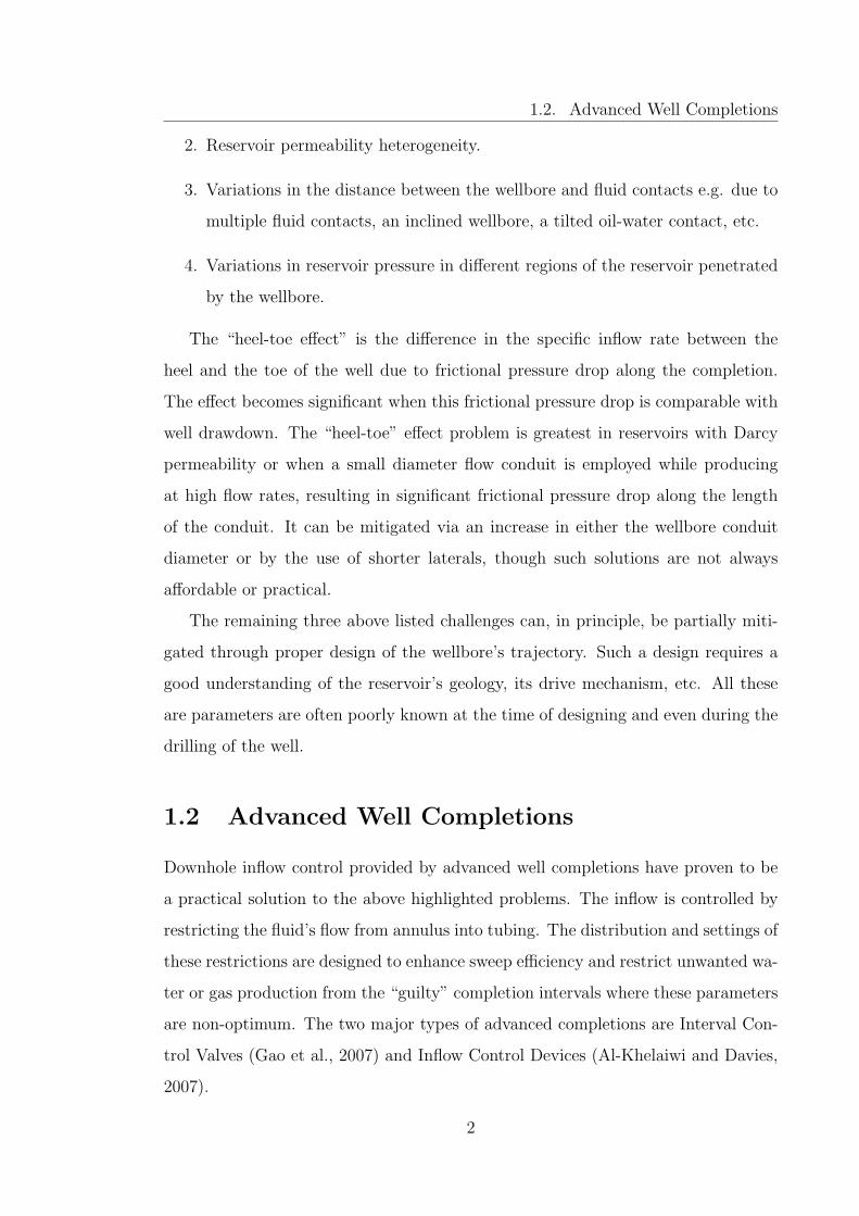
2. Reservoir permeability heterogeneity.
3. Variations in the distance between the wellbore and fluid contacts e.g. due to
multiple fluid contacts, an inclined wellbore, a tilted oil-water contact, etc.
4. Variations in reservoir pressure in different regions of the reservoir penetrated
by the wellbore.
The “heel-toe effect” is the difference in the specific inflow rate between the
heel and the toe of the well due to frictional pressure drop along the completion.
The effect becomes significant when this frictional pressure drop is comparable with
well drawdown. The “heel-toe” effect problem is greatest in reservoirs with Darcy
permeability or when a small diameter flow conduit is employed while producing
at high flow rates, resulting in significant frictional pressure drop along the length
of the conduit. It can be mitigated via an increase in either the wellbore conduit
diameter or by the use of shorter laterals, though such solutions are not always
affordable or practical.
The remaining three above listed challenges can, in principle, be partially miti-
gated through proper design of the wellbore’s trajectory. Such a design requires a
good understanding of the reservoir’s geology, its drive mechanism, etc. All these
are parameters are often poorly known at the time of designing and even during the
drilling of the well.
1.2 Advanced Well Completions
Downhole inflow control provided by advanced well completions have proven to be
a practical solution to the above highlighted problems. The inflow is controlled by
restricting the fluid’s flow from annulus into tubing. The distribution and settings of
these restrictions are designed to enhance sweep efficiency and restrict unwanted wa-
ter or gas production from the “guilty” completion intervals where these parameters
are non-optimum. The two major types of advanced completions are Interval Con-
trol Valves (Gao et al., 2007) and Inflow Control Devices (Al-Khelaiwi and Davies,
2007).
2

1.2. Advanced Well Completions
Interval Control Valve (ICV) is a key part of intelligent (or smart) well technol-
ogy. The completion interval of intelligent well is divided into zones by packers and
the inflow into each zone is controlled by an Interval Control Valve (Figure 1.1).
Hundreds of wells around the world are now equipped with remotely operated ICVs
of varying complexity and capabilities that are used to actively control inflow from
multiple completion intervals (zones) producing a common reservoir or from different
reservoirs.
Figure 1.1: Schematics of intelligent well (courtesy WellDynamics)
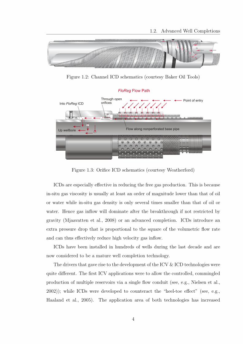
An Inflow Control Device (ICD) is a well completion screen that restricts the
fluid flow from the annulus into the base pipe. The restriction can be in form of
channels (Figure 1.2) or nozzles/orifices (Figure 1.3), but in any case the ability
of an ICD to equalise the inflow along the well length is due to the difference in
the physical laws governing fluid flow in the reservoir and through the ICD. Liquid
flow in porous media is normally laminar, hence the relationship between the flow
velocity and the pressure drop is linear. By contrast, the flow regime through an
ICD is turbulent, resulting in the quadratic velocity/pressure drop relationship.
The ICD’s resistance to flow depends on the dimensions of the installed nozzles
or channels. This resistance is often referred to as the ICD’s “strength”. It is set at
the time of installation and can not be adjusted without recompleting the well.
3
1.2. Advanced Well Completions
EQUA
LIZE
R™ is
Idea
l for
a W
ide
Rang
e of
App
licat
ions
Flui
d flo
w is
pro
mot
ed th
roug
h th
e sc
reen
, alo
ng th
e sc
reen
bas
e pi
pe
annu
lus,
into
the
helic
al IC
D. F
low
th
en e
nter
s th
e ba
se p
ipe
thro
ugh
a se
t of h
oles
or a
slo
tted
kill
filte
r.
MPa
s® E
QUAL
IZER
™ S
cree
n On
e-Tr
ip O
pen-
Hole
Com
plet
ion
A Un
ique
, Hel
ical
Inflo
w C
ontro
l Dev
ice
is th
e Ke
y to
EQ
UALI
ZER™
Effe
ctiv
enes
sA
hel
ical
Infl
ow C
ontr
ol D
evic
e (I
CD
) m
ount
ed to
the
base
pip
e at
the
end
of e
ach
scre
en e
nabl
es a
n eq
ual r
ate
ente
ring
eac
h sc
reen
alo
ng th
e en
tire
hori
zont
al s
ectio
n. T
his
has
prov
en to
be
by f
ar th
e m
ost e
ffec
tive
way
to
man
age
flow
dis
trib
utio
n al
ong
the
wel
lbor
e. T
his
is th
e fir
st ti
me
that
suc
h a
desi
gn h
as b
een
used
as
a lo
w-v
eloc
ity fl
ow c
ontr
ol e
lem
ent t
o ba
lanc
e in
flow
. Thi
s si
mpl
e so
lutio
n is
hig
hly
relia
ble,
imm
une
to e
rosi
on, a
nd it
s de
sign
ele
men
ts (
size
pitc
h, n
umbe
r of
cha
nnel
s) c
an b
e va
ried
to c
ontr
ol
the
loca
l pro
duct
ion
rate
at a
ny p
oint
alo
ng th
e w
ellb
ore.
Bec
ause
the
flow
co
ntro
l ele
men
t wor
ks in
a w
ide
vari
ety
of w
ell c
ondi
tions
, it i
s id
eal f
or
wel
ls w
here
con
ditio
ns c
hang
e ov
er ti
me.
Com
partm
enta
lize
Your
Wel
l with
Bak
er O
il To
ols
Form
atio
n Pa
cker
sB
y co
mbi
ning
EQ
UA
LIZ
ER
or
EQ
UA
LIZ
ER
CF
with
the
Bak
er O
il To
ols
MPa
s®, X
Tre
meZ
one®
, or
Rea
ctiv
e C
ore
Form
atio
n Pa
cker
s (R
CFP
),
you
com
part
men
taliz
e th
e w
ell a
nd e
nhan
ce th
e pe
rfor
man
ce o
f th
e E
QU
AL
IZE
R S
yste
m. C
ompa
rtm
enta
lizat
ion
also
allo
ws
for
com
min
gled
pr
oduc
tion
in w
ells
exh
ibiti
ng p
erm
eabi
lity
cont
rast
s, m
ultip
le z
ones
, or
vary
ing
rese
rvoi
r pr
essu
re. T
his
field
-pro
ven
appl
icat
ion
has
incr
ease
d oi
l pr
oduc
tion
rate
s an
d vo
lum
etri
c re
cove
ry f
rom
sev
eral
fiel
ds.
In h
oriz
onta
l ope
n ho
les,
E
QU
AL
IZE
R™
can
be
used
for
:
• A
void
ing
gas
brea
kthr
ough
• A
void
ing
wat
er b
reak
thro
ugh
• A
void
ing
sele
ctiv
e pe
rfor
atio
ns
• G
rave
l-pa
ck r
epla
cem
ent
• A
cid
dist
ribu
tion
equa
lizat
ion
• E
qual
izin
g ou
tflow
in e
xten
ded
inje
ctio
n w
ells
• L
ong,
hor
izon
tal w
ells
, esp
ecia
lly
thos
e w
ith h
oriz
onta
l run
s be
yond
1,5
00 f
t (45
0 m
)
• T
hin-
laye
red,
hig
h-pe
rmea
bilit
y re
serv
oirs
• H
eavy
-oil
rese
rvoi
rs
• St
and-
alon
e sc
reen
san
d co
ntro
l ap
plic
atio
ns
• C
onso
lidat
ed f
orm
atio
ns w
ith
earl
y ga
s or
wat
er b
reak
thro
ugh
Figure 1.2: Channel ICD schematics (courtesy Baker Oil Tools)
Figure 1.3: Orifice ICD schematics (courtesy Weatherford)
ICDs are especially effective in reducing the free gas production. This is because
in-situ gas viscosity is usually at least an order of magnitude lower than that of oil
or water while in-situ gas density is only several times smaller than that of oil or
water. Hence gas inflow will dominate after the breakthrough if not restricted by
gravity (Mjaavatten et al., 2008) or an advanced completion. ICDs introduce an
extra pressure drop that is proportional to the square of the volumetric flow rate
and can thus effectively reduce high velocity gas inflow.
ICDs have been installed in hundreds of wells during the last decade and are
now considered to be a mature well completion technology.
The drivers that gave rise to the development of the ICV & ICD technologies were
quite different. The first ICV applications were to allow the controlled, commingled
production of multiple reservoirs via a single flow conduit (see, e.g., Nielsen et al.,
2002)); while ICDs were developed to counteract the “heel-toe effect” (see, e.g.,
Haaland et al., 2005). The application area of both technologies has increased
4

1.3. The Scope of This Dissertation
dramatically since these early applications. Reservoir simulation and subsequent
field experience have confirmed that:
• ICV applications to a single reservoir add value (see, e.g., Brouwer and Jansen,
2004).
• ICDs can mitigate inflow or injection imbalance caused by permeability vari-
ations (see, e.g., Raffn et al., 2007).
1.3 The Scope of This Dissertation
This dissertation is focused on methodology of ICD completion design and justifi-
cation. Chapter 2 compares the functionality and applicability of ICD against the
competing ICV technology. Completion selection guidelines are developed based
on multiple criteria drawn from reservoir, production, operation and economic fac-
tors. Reservoir engineering aspects, such as uncertainty management, formation
heterogeneity, and the level of flexibility required by the development are analysed.
Production and completion characteristics, such as tubing size, the number of sep-
arately controllable completion zones, the installation of multiple laterals and the
value of real time information were also investigated. This systematic analysis forms
the basis of a screening tool to identify the optimum technology for each particular
situation.
This chapter provides a robust, comparative framework for both production tech-
nologists and reservoir engineers to select between passive (ICD) and active (ICV)
inflow control for optimised, advanced well completions.
Chapter 3 extends the ICD vs ICD comparison into the field of uncertainty anal-
ysis. It illustrates the quantification of the long-term benefits of advanced comple-
tions using the probabilistic approach and shows how advanced completions reduce
the impact of geostatistical uncertainty on the production forecast. Geostatistical
realisations of a benchmark reservoir model were generated with a suitable level of
data uncertainty. The reservoir was developed by a single horizontal well in a fixed
location. The probabilistic (P10, P50, P90) oil recovery distributions were then
5

1.3. The Scope of This Dissertation
obtained and compared for three completion options: an Open Hole with a sand
control screen or a perforated pipe, Inflow Control Devices (ICDs) and Interval
Control Valves (ICVs).
Steady-state performance of ICDs can be analysed in detail with well modelling
software (Ouyang and Huang, 2005; Johansen and Khoriakov, 2007). Most reservoir
simulators include basic functionality for ICD modelling; while some of them (Wan
et al., 2008; Neylon et al., 2009) also offer practical means to capture the effect of
the annulus flow. Thus, current numerical simulation software enables engineers to
perform the design and economic justification of an ICD completion. However we
hold a view that relatively simple analytical models still have a role to play in:
• Quick feasibility studies (screening ICD installation candidates).
• Verification of numerical simulation results.
• Communicating best practices in a non-product specific way.
Reduction of the “heel-toe effect” is one of the two main reasons for ICD applica-
tion. In order to find out whether particular well may benefit from ICD installation
one has to estimate frictional pressure losses along the completion. The flow regime
in most of horizontal wells is turbulent (Dikken, 1990). There are many publica-
tions on frictional pressure losses along the completion available in the literature,
but an explicit analytical solution for turbulent flow in wellbore has not so far been
published. Chapter 4 presents such a solution and thus helps to define the area of
ICD technology applicability.
Chapters 5 and 6 propose novel analytical models for reduction of inflow imbal-
ance caused by the “heel-toe effect” and reservoir heterogeneity respectively. These
models allow one to estimate the:
• ICD design parameters suitable for particular field application.
• Impact of ICD on the well’s Inflow Peformance Relationship (IPR).
The trade-off between well productivity and inflow equalisation is the key issue
of the ICD technology application. The proposed models quantitatively address this
issue. The practical utility of developed models is illustrated through case studies.
6

1.3. The Scope of This Dissertation
Chapter 7 presents the conclusions and possible extensions for this dissertation.
7
Chapter 2
How to Make the Choice between
Passive and Active Inflow-Control
Completions
2.1 Introduction
The application areas of the ICV and ICD technologies have developed so that
they overlap (Gao et al., 2007). We therefore initially studied the main functional
differences between ICVs and ICDs:
1. Remote control - ICVs deliver reservoir and production management advan-
tages giving more flexible field development, increased value of information,
improved clean-up etc.
2. Flow conduit diameter - The ICV’s reduced inner flow conduit diameter
increases the “heel-toe” effect compared to an ICD for comparable borehole
sizes.
3. Multilateral well applications - ICVs, unlike ICDs, can currently only
be installed in the well’s mother bore due to limitations of available control
8
2.2. Uncertainty in the Reservoir Description
umbilical technology to connect to both the mother bore and laterals at the
junction.
4. Design, Installation procedure complexity, Cost and Reliability -
ICV technology is more complex; hence ICDs have the advantage in terms of
simpler design and installation, and lower costs. Although the simplicity of the
ICD would imply greater reliability, there is little or no available operational
data to support this, particularly when considering the greater likelihood of
ICD plugging, due to scale, asphaltenes, waxes, etc., compared to ICVs.
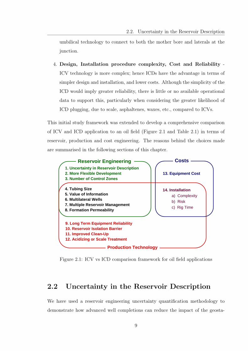
This initial study framework was extended to develop a comprehensive comparison
of ICV and ICD application to an oil field (Figure 2.1 and Table 2.1) in terms of
reservoir, production and cost engineering. The reasons behind the choices made
are summarised in the following sections of this chapter.
Reservoir Engineering
Production Technology
1. Uncertainty in Reservoir Description2. More Flexible Development3. Number of Control Zones
4. Tubing Size 5. Value of Information6. Multilateral Wells7. Multiple Reservoir Management8. Formation Permeability
9. Long Term Equipment Reliability10. Reservoir Isolation Barrier11. Improved Clean-Up12. Acidizing or Scale Treatment
Costs
13. Equipment Cost
14. Installationa) Complexity
b) Risk
c) Rig Time
Figure 2.1: ICV vs ICD comparison framework for oil field applications
2.2 Uncertainty in the Reservoir Description
We have used a reservoir engineering uncertainty quantification methodology to
demonstrate how advanced well completions can reduce the impact of the geosta-
9

2.2. Uncertainty in the Reservoir Description
Aspect ICD vsCased Hole
ICD vsICV
1. Uncertainty in Reservoir Description D V
2. More Flexible Development D V
3. Number of Controllable Zones D D
4. Inner Flow Conduit Diameter = D
5. Value of Information = V
6. Multilateral WellsControl of Lateral = V
Control within Lateral D D
7. Multiple Reservoir Management D V
8. Formation PermeabilityHigh D D
Medium-to-Low D V
9. Long Term Equipment Reliability C D
10. Reservoir Isolation Barrier = V
11. Improved Well Clean-Up D V
12. Acidizing/Scale Treatment D V
13. Equipment Cost D D
14. Installation D D
15. Gas Production C V
Table 2.1: Conventional cased hole, ICD and ICV completions compared
tistical uncertainty on the production forecast. The study results are summarised
below and described in detail in Chapter 3:
• ICD technology increased the mean recovery from 28.6% to 30.1% with a small
decrease in risk (P10 - P90) from 6.3% to 5.3%.
• ICV technology further increased the mean recovery to 30.6% and reduced the
risk compared to the base case by 50% (from 6.3% to 3.1%).
The impact of advanced completions on the probabilistic forecast of field oil
recovery was studied using 8 reservoir realisations of the PUNQ-S3 reservoir (Floris
10

2.3. More Flexible Development
et al., 2001). During this study it was found that the results were very dependent on
the choice of the Base Case. Advanced completions often add little or no value if the
degree of reservoir uncertainty is low and an optimum well trajectory is employed.
Our Base Case well design and completion was chosen using a relatively complete
knowledge of the reservoir, its geology, drive mechanisms and fluid contacts. Our
results represent a conservative estimate of the advanced completion’s value. This
is especially true for the ICV case.
2.3 More Flexible Development
An ICV’s downhole flow path’s diameter can be changed without intervention while
that for an ICD is fixed once it has been installed. The ICV thus has more degrees
of freedom than an ICD, allowing more flexible field development strategies to be
employed.
2.3.1 Reactive Control Based on “Unwanted” Fluid Flows
ICD completions restrict gas influx at the onset of gas breakthrough due to the
(relatively) high volumetric flow rate of gas. Nozzle (orifice) type ICDs can also
limit water influx due to the density difference between oil and water. However, an
ICD’s ability to react to unwanted fluids (i.e. gas and water) is limited compared to
that of an ICV, especially a multi-set point ICV. ICVs allow the well to be produced
at an optimum water or gas cut by applying the most appropriate (zonal) restrictions
which maximises the total oil production with a minimum gas or water cut.
2.3.2 Proactive Control
ICD completions impose a proactive control of the fluid displacing oil. However, it is
not possible to modify the applied restriction at a later date to achieve an optimum
oil recovery, even if measurements were available that indicated an uneven advance
of the flood front was occurring. ICVs, with their continuous flexibility to modify
the inflow restriction, have the advantage here (see, e.g., de Montleau et al., 2006).
11
2.4. Number of Controllable Zones
2.3.3 Real Time Optimization
Effective management of the reservoir sweep requires continuous adjustment of the
injection and production profiles throughout the well’s life. The continuous mea-
surement of downhole and surface data (e.g. pressure, temperature and flow rate)
in both injection and production wells, followed by the translation of this data into
information and, finally, the carrying out of actions based on this information that
require the ability to continuously adjust the fluid flow rate into or out of specific
wellbore sections (see, e.g., van den Berg, 2007). For example, maintaining the re-
quired production rate from a thin oil column or from a reservoir with a declining
pressure may require frequent flow rate adjustment (Meum et al., 2008). Similarly,
adjusting injection distribution may be required over time to account for changing
voidage replacement requirements. ICVs thus have the advantage here.
2.4 Number of Controllable Zones
The zonal flow length controlled by each ICV zone in horizontal and highly deviated
wells is normally large due to the technical and economic limitations of the number
of ICV that can be installed in a well. This limitation makes it difficult for ICVs
to control the movement of an advancing flood front towards a well completion con-
taining multiple sub-zones characterised by highly variable permeability values (e.g.
fractures, heterogeneous reservoir with a short, permeability correlation length). A
maximum of six ICVs have been installed in a well to date (Konopczynski, 2008).
Various electrical and hybrid electro-hydraulic systems have been developed with the
capability of managing many more valves per well. However, their high cost and op-
erating temperature limitations have precluded their widespread acceptance by the
market. The successful development of a low cost, reliable, single line, electrically-
activated valve will increase this maximum number of ICV-controlled zones that
can be installed in each well (Saggaf, 2008), though such a result will require radical
changes in current technology.
The number of zones controlled with ICDs is limited by the number of annular
12

2.5. Inner Flow Conduit Diameter
flow isolation packers employed and the incremental cost of the additional ICD’s
and packers. For example, Saudi Aramco suggests installing them every 50-100 ft
(Hembling et al., 2007). An ICD completion can thus potentially have many more
control zones than an ICV completion. This makes the ICD the potentially preferred
option for horizontal wells requiring many control intervals (e.g. wells completed in
a fractured or a heterogeneous reservoir with a short correlation length).
Dividing the wellbore into ten or more separate zones has become a practical
proposition since the development of swell packers (rings of rubber attached to the
screen joint that significantly increase their volume on exposure to water or oil (see,
e.g., Freyer and Huse, 2002; Ogoke et al., 2006)). Annular flow elimination is a
necessary condition for achieving the regulatory effect of ICDs installed across het-
erogeneous formations. It can most easily be achieved by installing swell packers;
though borehole collapse around the screen due to low formation strength or instal-
lation of a gravel pack (Augustine et al., 2008) can also reduce or eliminate annular
flow. A practical consideration for the selection of swell packers is the inability to re-
trieve the ICD/swell packer completion once the rubber has reacted. Thus, after an
ICD well has been completed, remedial mechanical actions to respond to problems
with this type of well is usually limited to borehole abandonment and sidetracking.
2.5 Inner Flow Conduit Diameter
2.5.1 Completion Sizes
The “heel-toe” effect is one of the two primary reasons for ICD installation. The
frictional pressure drop across a length of pipe is inversely proportional to the fifth
power of its internal diameter when the flow is turbulent (and to the fourth when
it is laminar). This strong dependence on the flow conduit diameter makes this
parameter an important factor when comparing the production performance of var-
ious completion designs, particularly for high flow rate wells. An ICD completion is
typically run in open hole. Its dimensions are often the same as that of the standard
sand screen for that hole size; the Outside Diameter (OD) of the flow conduit being
13
2.5. Inner Flow Conduit Diameter
Hole (bit) size, in. 5 7/8 7 7/8 8 1/2 or 9 1/2
Maximal ICD OD, in. 4 1/2 6 1/2 7 1/2
Flow ConduitOD, in. 3 1/2 5 1/2 6 5/8
ID, in. 3.0 4.9 5.9
Table 2.2: ICD completion sizes
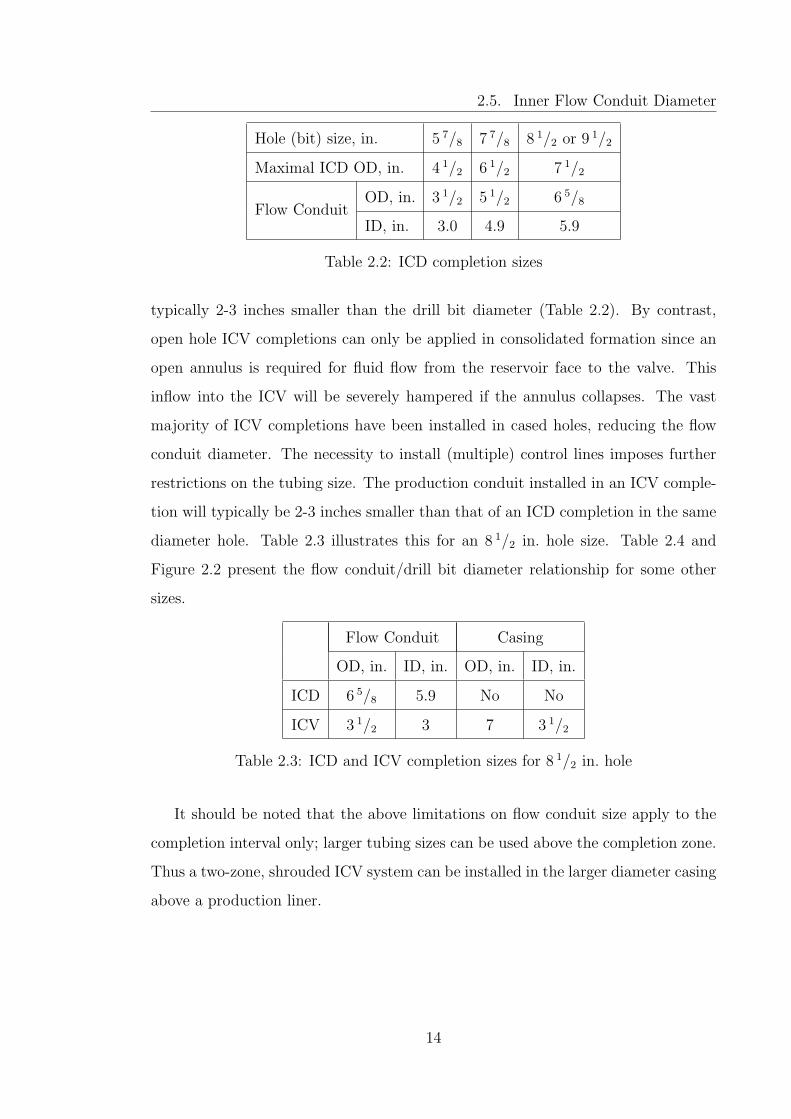
typically 2-3 inches smaller than the drill bit diameter (Table 2.2). By contrast,
open hole ICV completions can only be applied in consolidated formation since an
open annulus is required for fluid flow from the reservoir face to the valve. This
inflow into the ICV will be severely hampered if the annulus collapses. The vast
majority of ICV completions have been installed in cased holes, reducing the flow
conduit diameter. The necessity to install (multiple) control lines imposes further
restrictions on the tubing size. The production conduit installed in an ICV comple-
tion will typically be 2-3 inches smaller than that of an ICD completion in the same
diameter hole. Table 2.3 illustrates this for an 8 1/2 in. hole size. Table 2.4 and
Figure 2.2 present the flow conduit/drill bit diameter relationship for some other
sizes.
Flow Conduit Casing
OD, in. ID, in. OD, in. ID, in.
ICD 6 5/8 5.9 No No
ICV 3 1/2 3 7 3 1/2
Table 2.3: ICD and ICV completion sizes for 8 1/2 in. hole
It should be noted that the above limitations on flow conduit size apply to the
completion interval only; larger tubing sizes can be used above the completion zone.
Thus a two-zone, shrouded ICV system can be installed in the larger diameter casing
above a production liner.
14

2.5. Inner Flow Conduit Diameter
0
1
2
3
4
5
6
7
8
5 6 7 8 9 10 11
Hole Size, in
Tub
ing
Siz
e (O
D),
in
ICD ICV CASED hole ICV OPEN hole
Figure 2.2: ICD and ICV tubing sizes vs wellbore hole size
2.5.2 Impact of the Inner Flow Conduit Diameter on Inflow
Performance
Fluid flow is governed by pressure differences. An optimal design of an ICD com-
pletion requires a comparison of the pressure drop in the reservoir with that across
the ICD. These two values should be of the same order of magnitude (Table 2.5).
A reasonable level of inflow equalization can be achieved when the two pressure
drops are equal, thus ICD installation may be worthwhile if the “heel-toe” effect is
significant. A high level of inflow equalization requires the pressure drop across the
ICD to be several times greater than the pressure drop across the reservoir. These
simple considerations are in agreement with recommendations made by the major
ICD suppliers.
The most influential parameters for the ICD completion design are the well’s
PI – both the absolute value and its variation as a function of the location along
the wellbore, the length of the completion, the target drawdown or production rate
and the in-situ, reservoir fluid’s properties (density and viscosity). The optimum
ICD strength (i.e. nozzle diameter or pressure drop (“bar”) rating) for each par-
ticular well can be estimated using analytical formulae (Chapters 5 and 6); though
15
2.5. Inner Flow Conduit Diameter
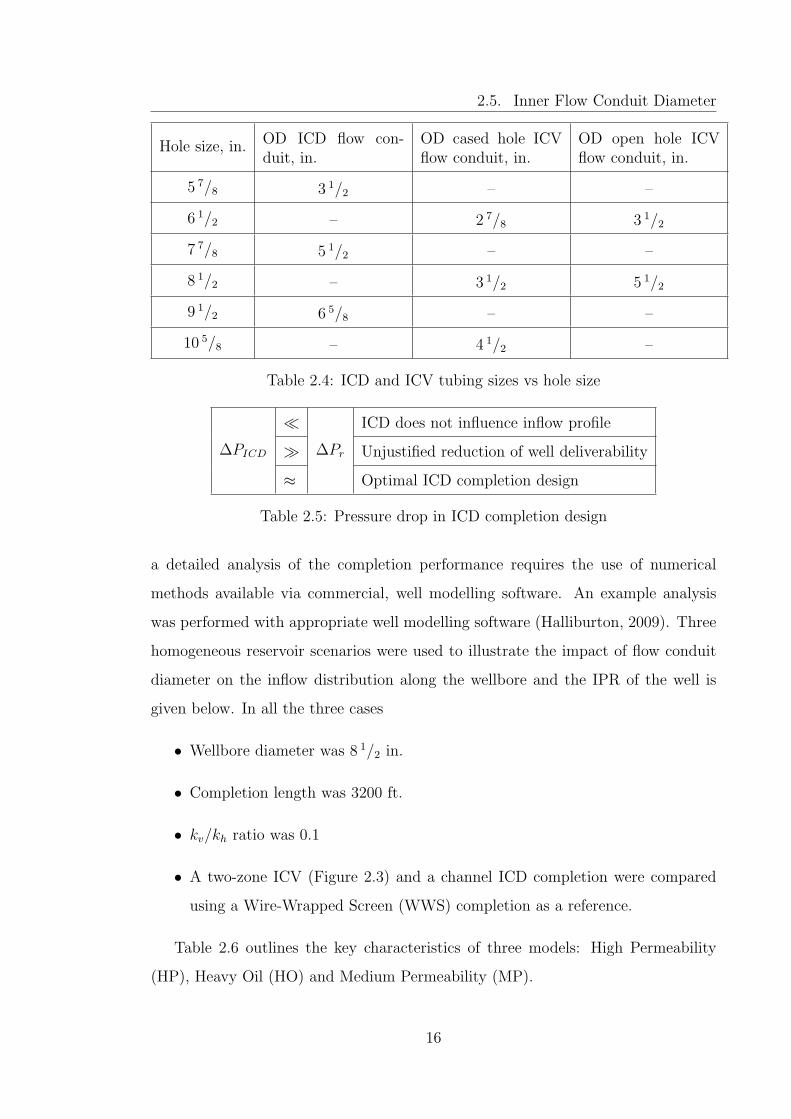
Hole size, in. OD ICD flow con-duit, in.
OD cased hole ICVflow conduit, in.
OD open hole ICVflow conduit, in.
5 7/8 3 1/2 – –
6 1/2 – 2 7/8 3 1/2
7 7/8 5 1/2 – –
8 1/2 – 3 1/2 5 1/2
9 1/2 6 5/8 – –
10 5/8 – 4 1/2 –
Table 2.4: ICD and ICV tubing sizes vs hole size
∆PICD
�∆Pr
ICD does not influence inflow profile
� Unjustified reduction of well deliverability
≈ Optimal ICD completion design
Table 2.5: Pressure drop in ICD completion design
a detailed analysis of the completion performance requires the use of numerical
methods available via commercial, well modelling software. An example analysis
was performed with appropriate well modelling software (Halliburton, 2009). Three
homogeneous reservoir scenarios were used to illustrate the impact of flow conduit
diameter on the inflow distribution along the wellbore and the IPR of the well is
given below. In all the three cases
• Wellbore diameter was 8 1/2 in.
• Completion length was 3200 ft.
• kv/kh ratio was 0.1
• A two-zone ICV (Figure 2.3) and a channel ICD completion were compared
using a Wire-Wrapped Screen (WWS) completion as a reference.
Table 2.6 outlines the key characteristics of three models: High Permeability
(HP), Heavy Oil (HO) and Medium Permeability (MP).
16
2.5. Inner Flow Conduit Diameter
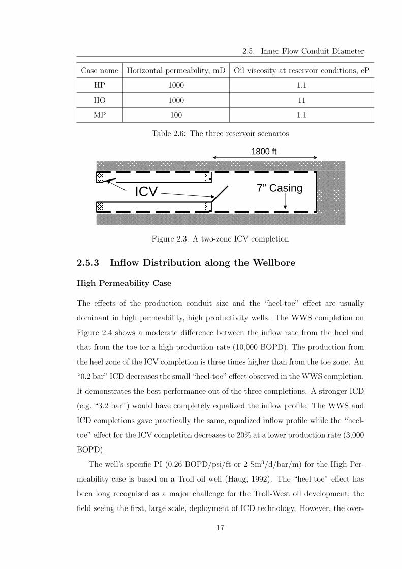
Case name Horizontal permeability, mD Oil viscosity at reservoir conditions, cP
HP 1000 1.1
HO 1000 11
MP 100 1.1
Table 2.6: The three reservoir scenarios
ICV 7” Casing
1800 ft
Figure 2.3: A two-zone ICV completion
2.5.3 Inflow Distribution along the Wellbore
High Permeability Case
The effects of the production conduit size and the “heel-toe” effect are usually
dominant in high permeability, high productivity wells. The WWS completion on
Figure 2.4 shows a moderate difference between the inflow rate from the heel and
that from the toe for a high production rate (10,000 BOPD). The production from
the heel zone of the ICV completion is three times higher than from the toe zone. An
“0.2 bar” ICD decreases the small “heel-toe” effect observed in the WWS completion.
It demonstrates the best performance out of the three completions. A stronger ICD
(e.g. “3.2 bar”) would have completely equalized the inflow profile. The WWS and
ICD completions gave practically the same, equalized inflow profile while the “heel-
toe” effect for the ICV completion decreases to 20% at a lower production rate (3,000
BOPD).
The well’s specific PI (0.26 BOPD/psi/ft or 2 Sm3/d/bar/m) for the High Per-
meability case is based on a Troll oil well (Haug, 1992). The “heel-toe” effect has
been long recognised as a major challenge for the Troll-West oil development; the
field seeing the first, large scale, deployment of ICD technology. However, the over-
17

2.5. Inner Flow Conduit Diameter
whelming majority of world’s oil wells have a productivity index at least one order
of magnitude lower than that encountered in Troll-West. The resulting reduction in
the “heel-toe” effect will be demonstrated with the next two cases.
0
1
2
3
4
5
6
7000 7500 8000 8500 9000 9500 10000 10500
Measured Depth, ft
Oil
Inflo
w,
ST
B /
d / f
t
WWS 10,000 STB/d
ICV 10,000 STB/d
0.2 bar ICD 10,000 STB/d
WWS 3,000 STB/d
ICV 3,000 STB/d
0.2 bar ICD 3,000 STB/d
Figure 2.4: High Permeability case, inflow from reservoir to well
Heavy Oil Case
The WWS and the ICD completion demonstrate a high level of inflow equalisation at
both the 3,000 and 10,000 BOPD production rates (Figure 2.5). The magnitude of
the “heel-toe” inflow ratio in the ICV completion is reduced to 1.5 times (compared
to 3 times in the High Permeability scenario). An increased oil viscosity decreases
the “heel-toe” effect. This occurs because the drawdown is proportional to viscosity
(Darcy’s law) while frictional pressure loss depends weakly on viscosity if the flow is
turbulent (as illustrated by the Moody diagram (Moody, 1944)). This combination
of parameters allows the drawdown to increase while the frictional pressure drop
remains almost the same. Hence the impact of frictional pressure drop on the inflow
profile will become smaller.
18

2.5. Inner Flow Conduit Diameter
0
0.5
1
1.5
2
2.5
3
3.5
4
7000 7500 8000 8500 9000 9500 10000 10500
Measured Depth, ft
Oil
Inflo
w,
ST
B /
d / f
t
WWS 10,000 STB/d
ICV 10,000 STB/d
0.2 bar ICD 10,000 STB/d
WWS 3,000 STB/d
ICV 3,000 STB/d
0.2 bar ICD 3,000 STB/d
Figure 2.5: Heavy Oil case, inflow from reservoir to well
Medium Permeability Case
A reduction in reservoir permeability increases the drawdown (at the same produc-
tion rate) while not influencing the pressure drop along the wellbore. Hence the
Medium Permeability (Figure 2.6) and Heavy Oil (Figure 2.5) cases show similar
results.
0
0.5
1
1.5
2
2.5
3
3.5
4
7000 7500 8000 8500 9000 9500 10000 10500
Measured Depth, ft
Oil
Inflo
w,
ST
B /
d / f
t
WWS 10,000 STB/d
ICV 10,000 STB/d
0.2 bar ICD 10,000 STB/d
WWS 3,000 STB/d
ICV 3,000 STB/d
0.2 bar ICD 3,000 STB/d
Figure 2.6: Medium Permeability case, inflow from reservoir to well
19

2.5. Inner Flow Conduit Diameter
2.5.4 Inflow Performance Relationship
Our well performance calculations employed the nodal analysis technique with the
node placed downstream of the completion. The WWS will thus have a better IPR
than the advanced completions since they introduce an additional pressure drop into
the fluid’s flow path from the reservoir to the tubing. In high permeability formations
the smaller diameter of the ICV completion’s flow conduit will frequently limit the
well’s production rate due to its poorer outflow performance.
Figure 2.7 shows the High Permeability case’s production performance based on
the IPR curves for the three completions types. The WWS demonstrates the best
inflow performance, as expected. The additional pressure drop imposed by the “0.2
bar” channel ICD is relatively small, its IPR is thus only slightly lower. The two-
zone ICV completion, with both valves fully open, takes “third place” in this IPR
comparison due to the smaller flow conduit diameter in the completion zone.
3340
3345
3350
3355
3360
3365
3370
0 2000 4000 6000 8000 10000 12000 14000 16000 18000
Oil Production Rate, STB/day
Flo
win
g B
otto
m H
ole
Pre
ssur
e, p
si Wire-Wrapped Screen
Both ICVs Open
Heel ICV closed
Toe ICV Closed
ICD 0.2 bar
ICD 3.2 bar
Outflow: 5.5"OD tubing, 310 psi THP
Figure 2.7: High Permeability case, impact of advanced completions on inflow per-formance
Shutting the heel ICV will (a) shorten the wellbore/reservoir exposure length by
forcing the fluid to flow the “long way” via the toe ICV and (b) reduce the inner
conduit diameter causing the total flow rate from the toe section to flow through the
20

2.6. Formation Permeability
smaller diameter tubing. The IPR for the ICV completion is thus the lowest of all.
The average flow path length becomes shorter when the toe valve closes, a scenario
that improves the inflow performance. The performance of the “3.2 bar” channel
ICD is similar to that of the ICV completion with the toe ICV closed. The overall
conclusion is that the larger flow conduit diameter gives the ICD an advantage over
ICV. This advantage plays an important role in high permeability, high production
rate applications.
2.6 Formation Permeability
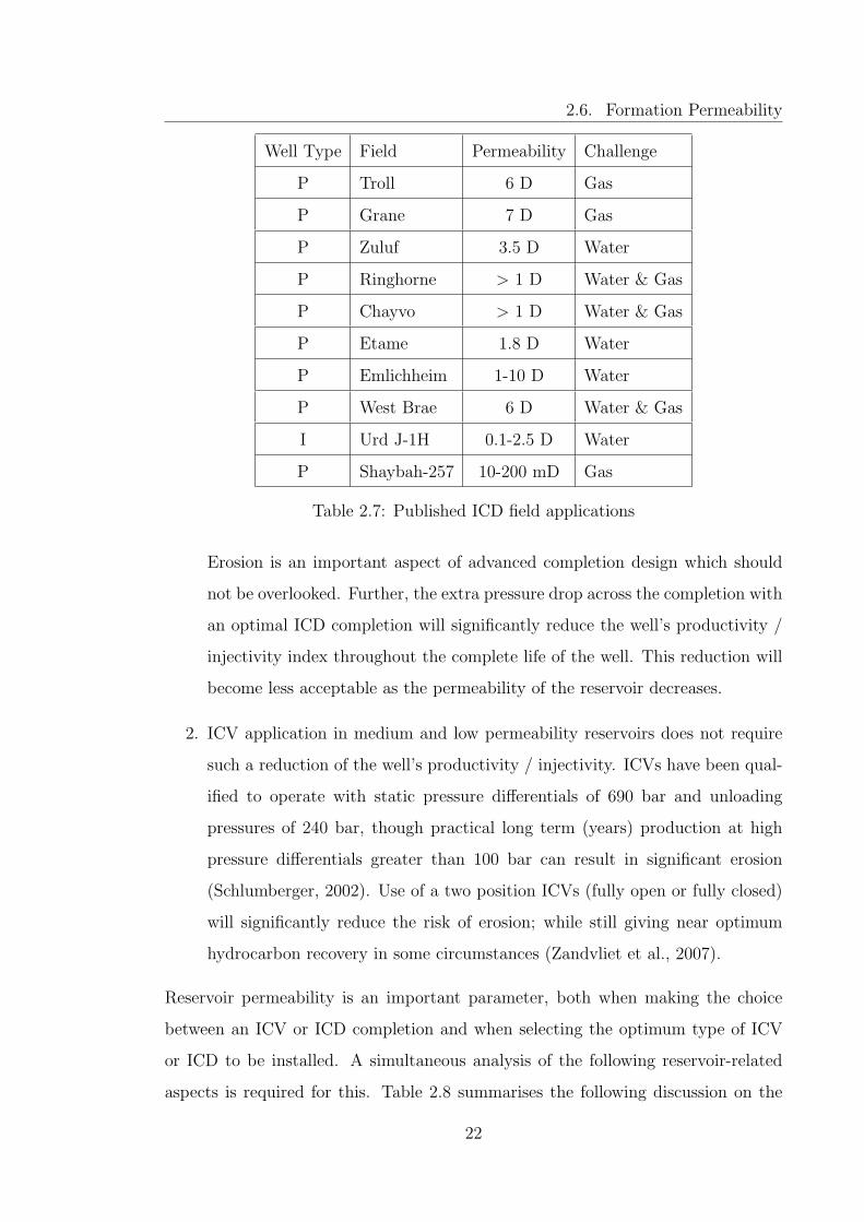
Table 2.7, a compilation of published ICD field applications, shows that they have
been mainly applied to reservoirs with an average permeability of one Darcy or
greater, the only exception being the Shaybah field (Salamy et al., 2006) where
ICDs were applied to reduce the production of free gas from the gas cap. The
requirement to create a completion pressure drop similar to the reservoir drawdown
has two important consequences with respect to ICD applications in medium and
low permeability reservoirs:
1. Low permeability reservoirs are normally produced at a higher drawdown
than more permeable reservoirs; hence an ICD employed in such a field must
also generate high pressure drop for effective equalisation while being suffi-
ciently robust to withstand both the high pressure drop and, possibly, a high
flow velocity throughout the well’s active life. Any erosion (enlargement) of
the ICD restriction will reduce inflow equalisation. Erosion is expected to pref-
erentially occur at higher permeability zones in heterogeneous formations due
to their higher production potential and weaker formation strengths. Selective
erosion could thus reduce the pressure drop across the high permeability zone
while it maintains that across the low permeability zones restriction. The
level of flow equalisation will then be reduced. It is expected that suitable
equipment design and proper choice of construction materials will mitigate
this concern, as has been achieved for ICVs (Gao et al., 2007).
21
2.6. Formation Permeability
Well Type Field Permeability Challenge
P Troll 6 D Gas
P Grane 7 D Gas
P Zuluf 3.5 D Water
P Ringhorne > 1 D Water & Gas
P Chayvo > 1 D Water & Gas
P Etame 1.8 D Water
P Emlichheim 1-10 D Water
P West Brae 6 D Water & Gas
I Urd J-1H 0.1-2.5 D Water
P Shaybah-257 10-200 mD Gas
Table 2.7: Published ICD field applications
Erosion is an important aspect of advanced completion design which should
not be overlooked. Further, the extra pressure drop across the completion with
an optimal ICD completion will significantly reduce the well’s productivity /
injectivity index throughout the complete life of the well. This reduction will
become less acceptable as the permeability of the reservoir decreases.
2. ICV application in medium and low permeability reservoirs does not require
such a reduction of the well’s productivity / injectivity. ICVs have been qual-
ified to operate with static pressure differentials of 690 bar and unloading
pressures of 240 bar, though practical long term (years) production at high
pressure differentials greater than 100 bar can result in significant erosion
(Schlumberger, 2002). Use of a two position ICVs (fully open or fully closed)
will significantly reduce the risk of erosion; while still giving near optimum
hydrocarbon recovery in some circumstances (Zandvliet et al., 2007).
Reservoir permeability is an important parameter, both when making the choice
between an ICV or ICD completion and when selecting the optimum type of ICV
or ICD to be installed. A simultaneous analysis of the following reservoir-related
aspects is required for this. Table 2.8 summarises the following discussion on the
22

2.6. Formation Permeability
impact of reservoir permeability on the choice between an ICV and an ICD:
1. Inflow control objectives. An optimal development strategy does not always
require complete uniformity of inflow that an ICD can provide. Thus flow
equalization might not be required if the distance between the wellbore and
aquifer (or injector) varies significantly for different parts of a long horizontal
well. The required degree of inflow equalization must be determined if inflow
equalization is not the sole control objective.
2. Well performance. A high ICD strength may be needed to achieve a high level
of inflow uniformity, reducing the overall well productivity / injectivity. A
compromise between these two criteria must be sought.
3. Fluid phases involved (oil, water, gas).
(a) Both ICVs and ICDs can be used to manage gas flow distribution in a
gas injection completion. ICD application to gas injection in oil fields is
unlikely to pose:
• erosion concerns since the injected gas is normally dry, sand-free and
non-corrosive;
• injectivity loss concerns since the viscosity of the gas at reservoir
conditions is at least an order of magnitude lower than that of oil
or water hence gas injectivity (in reservoir volumes) is considerably
higher than that of water.
(b) Limiting water production in a low permeability reservoir with an ICD
presents practical difficulties due to the resulting high pressure drop
across the completion.
(c) ICDs can be useful in reducing volume of gas cap gas produced in low
permeability fields. The ICD’s pressure drop is proportional to the square
of the volumetric flow rate; while the in-situ gas density is several times
smaller than that of oil or water. Downhole, gas flow velocities are greater
than those experienced during liquid production, hence an ICD than will
restrict gas production more efficiently by water production.
23

2.7. Value of Information
(d) High viscosity emulsions can form within advanced completions incor-
porating a small diameter flow restriction. Emulsion formation depends
on which surface active components present within the crude oil and the
shear experienced by the fluid mixture during flow through the restriction.
The emulsion can increase the fluid’s viscosity several times, reducing the
well’s outflow performance.
4. Production / injection rate. The relationship between the pressure drop and
the flow rate is linear for liquid flow in the reservoir and quadratic within the
ICD. The ratio of these pressure drops, and ultimately the completion design,
thus depends on the well’s production or injection rate. The efficiency of the
ICD will decrease if the well operates at a different flow velocity from the value
for which the ICD completion was designed. Appropriate sensitivity analyses
should study the implication of expected / possible flow velocity changes on
the ICD completion’s performance.
5. Productivity variations along the wellbore. An ICD allows many intervals to
be controlled along the inflow zone - though high permeability contrasts can
be difficult to smooth out with a constant strength, ICD completion.
2.7 Value of Information
Downhole pressure, temperature and flow rate measurements can now be made avail-
able on a real time basis due to advances in fiber optic sensing technology. This
technology can be applied to conventional as well as advanced (ICD and ICV) com-
pletions. Measurements can be made both outside the completion (at the sandface)
and within the flow conduit. Analysis of this data improves the surveillance engi-
neer’s understanding of the subsurface processes. Any required remedial actions can
thus be more quickly identified and implemented based on up-to-date well data.
The ICV’s advantages with respect to “Value of Information” stems from its
remote control capability. Changing the well’s total production rate via the surface
choke is the only action that can be taken with conventional and ICD completions;
24
2.8. Multilateral Wells
Inflow Control Devices Interval Control Valves
Pro
lific
rese
rvoi
rs
Oilproducer
Prevent early water & gas break-through (+)
Similar to ICD (+) butsmall tubing size restrictsproduction or injectionrate. Can be mitigated bydrilling larger hole (–).Gas/water
injectorEqualise injection profile (+)
Med
ium
and
low
per
-m
eabilit
yre
serv
oirs
Oilproducer
Reduce gas-liquid ratio (+). Wa-ter cut not reduced (–).
Reduce both GLR andwater cut (+)
Gas/waterinjector
Suitable for gas injection (+).Application for water injectionrequires larger injection pressureto overcome ICD pressure loss (–) and erosion resistant ICD de-sign (–).
Suitable for both waterand gas injection (+).Small tubing size impor-tant if injection rate ishigh (–).
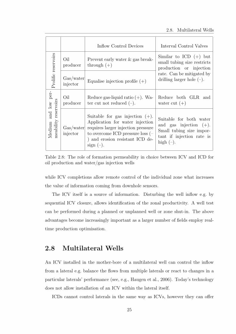
Table 2.8: The role of formation permeability in choice between ICV and ICD foroil production and water/gas injection wells
while ICV completions allow remote control of the individual zone what increases
the value of information coming from downhole sensors.
The ICV itself is a source of information. Disturbing the well inflow e.g. by
sequential ICV closure, allows identification of the zonal productivity. A well test
can be performed during a planned or unplanned well or zone shut-in. The above
advantages become increasingly important as a larger number of fields employ real-
time production optimisation.
2.8 Multilateral Wells
An ICV installed in the mother-bore of a multilateral well can control the inflow
from a lateral e.g. balance the flows from multiple laterals or react to changes in a
particular laterals’ performance (see, e.g., Haugen et al., 2006). Today’s technology
does not allow installation of an ICV within the lateral itself.
ICDs cannot control laterals in the same way as ICVs, however they can offer
25

2.9. Multiple Reservoir Management (MRM)
inflow control along the length of the lateral (Qudaihy et al., 2006). The different
flow control capabilities offered by ICVs and ICDs result in both technologies being
employed in multilateral wells (see, e.g., Sunbul et al., 2007).
2.9 Multiple Reservoir Management (MRM)
Simultaneously accessing multiple reservoirs from the same wellbore yields reduced
capital and operational expenditure for field development. Both national petroleum
legislation and good reservoir engineering practice require allocation of the field’s or
well’s total daily production to a particular zone as well as prevention of reservoir
cross-flow. The advantages of MRM are:
• Optimal sequential production (Akram et al., 2001)
• Commingled production via a single wellbore (see, e.g., Nielsen et al., 2002)
• Controlled fluid transfer between layers (for sweep improvement or pressure
support) (Lau et al., 2001)
• In-situ (auto) gas lift (see, e.g., Al-Kasim et al., 2002)
• Prevention of cross flow between reservoirs during periods of well shut-in or low
rate production. Such cross flow can damage reservoirs due to incompatibility
of fluids or changing the fluid saturation levels of the rock as well as can
resulting in loss of reserves to low pressure reservoirs.
These advantages have been achieved in the field with ICV completions. ICD
MRM applications have not yet been published, although ICDs are capable, in prin-
ciple, of limiting cross-flow due to the imposed additional, flow resistance. They are
not capable of preventing cross flow between reservoirs. A dual completion (Fig-
ure 2.8) is the conventional solution for simultaneous management of two reservoir
layers; while a Single-string, ICV completion (Figure 2.9) is the “advanced” option.
A 121/4 in. hole, 95/8 cased well can be completed with two 31/2 tubing strings (a
dual completion) or a 5 1/2 in. flow conduit with ICVs (the advanced completion).
26

2.10. Long Term Equipment Reliability
ICVs have the advantage over ICDs for MRM (Table 2.9). This is well known as
commingling was one of the original drivers behind many ICV installations.
Figure 2.8: Multiple layer reservoir management with dual completion
CompletionOptimalsequentialproduction
ComminglingControlledfluid flow be-tween layers
In-situ gas lift
Dual comple-tion
+ + – –
ICV + + + +
Table 2.9: Interventionless production of a two layer reservoir of a conventional dualand a single string ICV completions compared
2.10 Long Term Equipment Reliability
Erosion or plugging of nozzle or channel in principle can cause ICD failure; however
data on ICD reliability is not publicly available. There has been some field evidence
of screen plugging during ICD installation.
An ICV is a more complex piece of equipment than an ICD, making it potentially
less reliable. ICV failure is usually defined as the “inability to cycle the valve to
27
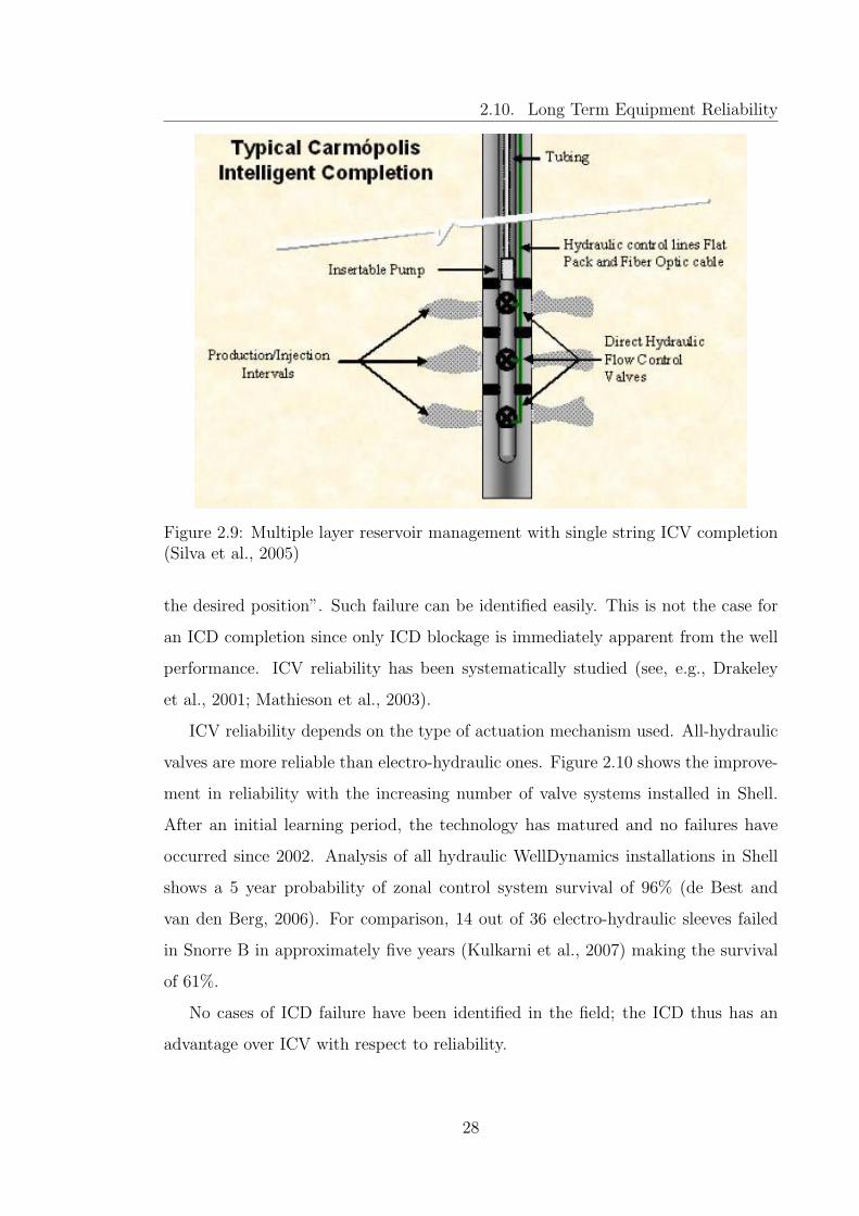
2.10. Long Term Equipment Reliability
Figure 2.9: Multiple layer reservoir management with single string ICV completion(Silva et al., 2005)
the desired position”. Such failure can be identified easily. This is not the case for
an ICD completion since only ICD blockage is immediately apparent from the well
performance. ICV reliability has been systematically studied (see, e.g., Drakeley
et al., 2001; Mathieson et al., 2003).
ICV reliability depends on the type of actuation mechanism used. All-hydraulic
valves are more reliable than electro-hydraulic ones. Figure 2.10 shows the improve-
ment in reliability with the increasing number of valve systems installed in Shell.
After an initial learning period, the technology has matured and no failures have
occurred since 2002. Analysis of all hydraulic WellDynamics installations in Shell
shows a 5 year probability of zonal control system survival of 96% (de Best and
van den Berg, 2006). For comparison, 14 out of 36 electro-hydraulic sleeves failed
in Snorre B in approximately five years (Kulkarni et al., 2007) making the survival
of 61%.
No cases of ICD failure have been identified in the field; the ICD thus has an
advantage over ICV with respect to reliability.
28

2.11. Reservoir Isolation Barrier
Figure 2.10: ICV reliability statistics for all-hydraulic systems (de Best and van denBerg, 2006)
2.11 Reservoir Isolation Barrier
An ICV has been accepted as reservoir isolation barrier during the initial stages of
well intervention operations e.g. removal of wellhead (Stair et al., 2004). This reduces
the required rig time and lowers the cost of the intervention. Another advantage is
that the reservoir is not exposed to the workover fluid, reducing the risk of formation
damage.
An ICD can not act as an isolation barrier.
29

2.12. Improved Well Clean-Up
2.12 Improved Well Clean-Up
Formation damage frequently significantly reduces well performance to a value be-
low the well’s “real” potential. Well clean-up is the process by which this damage
may be removed. This is a particularly important issue in a low permeability en-
vironment. There is no available quantitative model of clean-up process, but an
increased drawdown has proven to be successful (and has been observed by DTS).
Sequential opening and closing of valves allows imposing higher drawdown on one
zone after another. Thus ICV technology provides better clean-up than conventional
completion.
The effect of ICD on clean-up is ambiguous. On one hand, ICD the maximum
reservoir drawdown that can be applied will be reduced due to the choking effect
of the completion (and the quadratic relationship between flow rate and pressure
drop across ICD). On the other hand, the ICD equalises inflow. Hence, clean-up of
the high productive and the heel intervals will be restricted, allowing a (relatively)
greater drawdown – and better clean-up – of the remainder of the well. Which of
these two factors will prevail depends on particular circumstances such as availability
(and power) of artificial lift.
Due to above mentioned reasons I believe that ICVs will have advantage over
ICDs in terms of clean-up in most of practical situations.
It should be noted, however, that it is an emerging area of research: large number
of publications have addressed this question during last several years (see, e.g., Moen
and Asheim, 2008; Sunbul et al., 2008; Al-Khelaiwi et al., 2009; Olowoleru et al.,
2009; Shahri et al., 2009). The debate is still open.
2.13 Bullhead Selective Acidizing or Scale Treat-
ment
Correct placement of acid or inhibitor is crucial for success of acidizing or scale
treatment jobs in long horizontal wells. Difficulties in placement increase with well
length and permeability variations. It is impossible to treat long completion intervals
30

2.14. Equipment Cost
when the injection rate is too low. ICDs have advantage over conventional well in
terms of acidizing and scale treatment due to their equalizing effect. ICVs can focus
the treatment precisely on the target zone (Bellarby et al., 2003; Kavle et al., 2006),
providing better placement and more economical use of the chemical agent compared
to an ICD.
2.14 Equipment Cost
Completion costs vary greatly depending on the required functionality. The more
complex nature of an ICV completion (compared to an ICD) results in the ICV
being more expensive than the ICD in almost all cases. Similarly the ICD will be
more expensive than a wire-wrapped screen.
A 5 1/2 inch ICD completion for 4800 ft horizontal well in 2002 was reported
to cost $1.8 million (Augustine, 2002), a sum what was approximately 30% greater
than a generic sand screen completion. Typical ICV completions would cost several
million US dollars. Low (many tens or hundreds of thousands of USD) cost ICV
applications have been reported (Silva et al., 2005). ICV equipment is more expen-
sive than alternative ICD hardware. Quantitative comparison of ICV vs ICD costs
is difficult to perform as these costs are very case specific and not publicly available.
2.15 Installation
ICV completion is more expensive in terms of installation complexity, rig time and
installation risks. The last can be mitigated by proper planning and training as well
as through system integration tests.
2.16 Gas Fields
The context of the above comparison is oil production, the current arena of ICV-
ICD competition. However the same guidelines can be used for gas field applications,
complemented by the following “gas specific” reasoning.
31
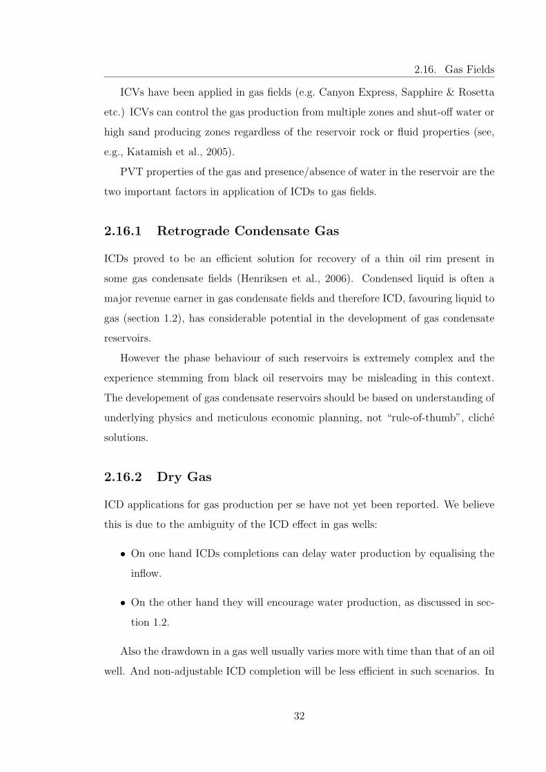
2.16. Gas Fields
ICVs have been applied in gas fields (e.g. Canyon Express, Sapphire & Rosetta
etc.) ICVs can control the gas production from multiple zones and shut-off water or
high sand producing zones regardless of the reservoir rock or fluid properties (see,
e.g., Katamish et al., 2005).
PVT properties of the gas and presence/absence of water in the reservoir are the
two important factors in application of ICDs to gas fields.
2.16.1 Retrograde Condensate Gas
ICDs proved to be an efficient solution for recovery of a thin oil rim present in
some gas condensate fields (Henriksen et al., 2006). Condensed liquid is often a
major revenue earner in gas condensate fields and therefore ICD, favouring liquid to
gas (section 1.2), has considerable potential in the development of gas condensate
reservoirs.
However the phase behaviour of such reservoirs is extremely complex and the
experience stemming from black oil reservoirs may be misleading in this context.
The developement of gas condensate reservoirs should be based on understanding of
underlying physics and meticulous economic planning, not “rule-of-thumb”, cliche
solutions.
2.16.2 Dry Gas
ICD applications for gas production per se have not yet been reported. We believe
this is due to the ambiguity of the ICD effect in gas wells:
• On one hand ICDs completions can delay water production by equalising the
inflow.
• On the other hand they will encourage water production, as discussed in sec-
tion 1.2.
Also the drawdown in a gas well usually varies more with time than that of an oil
well. And non-adjustable ICD completion will be less efficient in such scenarios. In
32

2.17. Conclusions
principle, perforating (after water breakthrough) can convert ICD completion into
a conventional slotted liner but this raises new concerns:
• Delayed production.
• Optimal moment for perforation may be not obvious since different completion
intervals may exhibit different behaviour.
• Health, safety and environmental risks.
Thus, in case of dry gas production, water breakthrough deprives an ICD of one
of its main advantages over an ICV – its simplicity.
2.16.3 Wet Gas
Phase behaviour of wet gas is somewere between that of a condensate and a dry
gas. Liquids may condense in the completion zone and/or the wellbore depend-
ing on the produced fluid’s PVT envelope, reservoir pressure and temperature and
the conditions of flow through the ICD. A completion enhancing production of the
liquid fraction may be either desirable or undesirable depending on particular cir-
cumstances (economics, lifting capability of the well, etc.). The value of ICDs in
wet gas field applications requires additional investigation and is beyond the scope
of this dissertation.
2.17 Conclusions
Major aspects dictating the choice between ICVs and ICDs have been reviewed.
Figure 2.1 and Table 2.1 provide basis for the selection criteria. The value differ-
ence between ICV and ICD has been quantified where appropriate. As usual, full
economic quantification of the value associated with each completion remains a field
specific task.
33

Chapter 3
Impact of Reservoir Uncertainty
on Selection of Advanced
Completion Type
3.1 Introduction
Well performance prediction is one of the major tasks when preparing an oil or gas
field development plan. The complexity and predictive quality of models used to
support this activity have increased significantly during the last two decades, partly
driven by the ever decreasing cost coupled with the increasing power of computers
However, large discrepancies between the model and reality still frequently occur.
They stem from:
• The lack of data (e.g. the unknown distribution of petrophysical properties in
reservoir).
• Deliberate simplifications to make the problem more tractable (e.g. upscaling,
black oil PVT models, neglect of thermal effects, etc.).
• Computational (sub-grid) errors and
34

3.1. Introduction
• An incomplete understanding of the physics and chemistry of the subsurface.
Petroleum researchers still work on developing more precise description of the
laws governing hydrocarbon production (e.g. multiphase flow, relative perme-
ability effects associated with gas condensate flow in porous media, effect of
water salinity on oil recovery, etc.).
Many E&P development decisions are made under a high level of uncertainty.
The degree of uncertainty and its impact on decision making is naturally greatest
at the exploration stage of the field development process. This is one reason why
a probabilistic analysis is part of reserves estimation and other standard workflows
used in making early development decisions. The predictive accuracy of reservoir
models should increase as the field development proceeds, since the quality and
the quantity of reservoir data will continually increase. Reservoir models should
be continually updated by field production data, history matching, and the ever
increasing number of (logged) reservoir penetrations. However, uncertainty quan-
tification always remains an important task; even during the later, more mature
phase of reservoir development.
Reservoir engineers typically deal with multiple possible reservoir models of the
real field. A single, or several, possible development strategies are evaluated and
compared using all these models. The results of multiple simulations are processed to
quantify the uncertainty in the production forecast. Special software tools (Schulze-
Riegert et al., 2001; Manceau et al., 2001; Williams et al., 2004) have been developed
to assist reservoir engineers in managing the required large number of reservoir
simulations, the processing of their results and, ultimately, the quantifying of the
uncertainty in the production forecast.
The parameters used in well completion design (e.g. well productivity index,
deviation and skin, fluid composition, reservoir pressure etc.) can normally be mea-
sured or estimated more precisely than the macro-scale, reservoir characteristics
which describe the complete reservoir. Completions are traditionally designed using
well performance software which employs a reservoir inflow description that is often
only valid over a short period at a particular pointing time during the reservoir’s
35

3.1. Introduction
exploitation. Systematic implementation of the probabilistic approach to decision
making, as is widely practised in Reservoir Engineering and Geoscience, has rarely
been used in completion modeling where wellbore and near-wellbore parameters are
typically used in a deterministic manner to choose the optimum tubing and casing
dimensions, the well construction materials, the perforation density etc.
Vertical and slightly deviated (or conventional) wells commonly have a relatively
small reservoir contact length. This limited length allows reservoir drainage control
to be implemented by adjusting the production or injection rate of individual wells
with a surface choke. Such an optimum reservoir drainage strategy will enhance
the reservoir sweep efficiency and limit production of unwanted water or gas. The
project’s profitability will thus be enhanced along with other, long term, economic
benefits.
Horizontal wells are characterised by a greatly increased reservoir contact com-
pared to conventional wells. Surface control of the well’s production is no longer
sufficient, on its own, to implement an optimum reservoir drainage strategy. Ad-
vanced completions, with their control of the reservoir fluid inflow along the length
of (long) completion interval, were developed to overcome this challenge.
Conventional well performance simulators and mechanical engineering packages
have proven to be sufficient to address the major design issues associated with
conventional completions, such as the:
• Well’s ability to deliver a target production rate.
• Balance between reservoir inflow and tubing outflow within the well and
• Mechanical issues (e.g. sand-control, equipment reliability, etc.)
An evaluation of the (economic) benefit of the chosen, conventional well, com-
pletion design is traditionally based on a series of short term predictions (or “snap-
shots”) of well performance at various periods in the well’s life. (The input reservoir
performance parameters are normally supplied by simulation or other reservoir engi-
neering techniques e.g. material balance.) In addition, a simple sensitivity analysis
is often carried out to evaluate the “robustness” of the chosen design if “possible”
36

3.1. Introduction
values for the above parameters are found to occur. However, a systematic analysis
of realistic combinations of these parameters is not normally performed.
Justification of an advanced completion is a more complex process since the
completion can react to the reservoir’s inflow performance by adjusting its outflow.
The significantly greater cost of the advanced completion along with its dynamic
adjustment of the well’s performance requires that the long term economic benefits
should be analysed when considering installing an advanced completion. The com-
pletion’s dynamic interaction with the reservoir displacement processes implies that
a software tool that closely couples the simulation of the reservoir with an accurate
description of the well performance is required to quantify these economic benefits.
These benefits can then be expressed in terms of the cumulative oil production, risk
reduction, etc. or in the standard economic terms such as net present value, internal
rate of return, etc.
This combination of reservoir and wellbore modeling, economic evaluation and,
sometimes, a sophisticated optimization routine are required to:
• Choose the number and location of inflow control zones.
• Make optimum use of the advanced completion’s ability to adjust itself through-
out the well’s life to maximize the economic performance.
• Assess the economic implications of any reduction in the reliability of an ad-
vanced wells, more complex, completion components compared to that of a
conventional well.
• Justify the extra cost of the advanced completion (compared to conventional
one) to (a possibly sceptical) management.
The design of advanced completions thus requires an integrated knowledge of
both well and reservoir technology.
Uncertainty quantification is an important and well established part of the reser-
voir engineering skill set. The remainder of Chapter 3 will show how the same ap-
proach can be used to design an advanced completion that can perform efficiently
despite the uncertainty reflected by a range of possible reservoir models.
37

3.2. Literature Review
3.2 Literature Review
The impact of reservoir uncertainty on the selection of completion system has his-
torically been addressed from several perspectives:
1. Wehunt (2006) presented a probabilistic distribution of skin values for three
common completion types. These distributions were based on several hun-
dred observations of vertical or slanted wells. The impact of other uncertain
parameters was analyzed and the Monte Carlo technique used to assess their
impact on the estimated well productivity.
2. Ouyang (2007) considered five common completion scenarios for a horizontal
well in homogeneous formation. He performed a sensitivity study of the oil
production rate with respect to both the completion type and the reservoir
characteristics. The study illustrated that “uncertainty in input parameters
may play an important role in well completion modeling and well performance
prediction”.
Well Inflow Performance analysis of conventional completions has normally em-
ployed a simple “snap-shot-in-time” approach in which the reservoir was represented
by a single value of the productivity index, reservoir pressure and phase fractions.
The traditional reluctance to use reservoir simulation in the evaluation of conven-
tional completion performance is exemplified by the above two papers – they both
included it as an optional rather than a compulsory step.
Advanced completions can be seen as an additional investment which “pays back”
by improving the long term project economics through an increased operational
flexibility. Sharma et al. (2002) and Han (2003) suggested applying real options
theory to quantify the value of the flexibility offered by advanced completions. The
key parameters for Real Options evaluation process are the present value of the
project and its accompanying Uncertainty. These parameters can only be estimated
via multiple reservoir simulations. Both these publications focus on the application
of the real options concept rather than on the reservoir engineering aspects of the
problem that are addressed in this chapter.
38

3.3. Advanced Well Completions
Real options analysis is a mathematical theory that allows the financial compar-
ison of the risk and reward associated with a number of possible strategies, each
of which is made-up of a portfolio of several possible investment opportunities or
projects. Traditional Net Present Value evaluation methods use a predefined, fixed
project scenario that does not quantify the value of flexibility that can allow a reduc-
tion in the level of uncertainty while maintaining the expected reward. The source of
real options theory was the evaluation and optimisation of a range of possible port-
folios of shares against a specified level of risk or uncertainty. Such an application
naturally translates to the building of an optimum portfolio of multiple exploration
licenses, each having a separate value and associated risk along with the right, but
not the obligation, to develop a possible discovery.
A number of attempts have been made to popularize the real options theory
within the petroleum industry. However, even financial experts (Leslie and Michaels,
1997) admit that “options theory is notoriously arcane” and “many discussions that
go beyond the conceptual level get bogged down in the mathematics”. Real options
theory is still far from being accepted by petroleum industry as a standard evaluation
method (Gai, 2002). Further, the necessary software is not widely available within
the industry.
This chapter addresses the reservoir engineering aspects of obtaining the key
input parameters for a real options evaluation. Completion technologies will be
compared in terms of their impact on probabilistic distribution of oil recovery (P50,
P90 and P10). It will be shown that the main objective of this comparison - to
demonstrate how advanced completions can reduce the impact of geostatistical un-
certainty on production forecasting - can be fulfilled without going into the depths
of real options theory.
3.3 Advanced Well Completions
Both ICVs and ICD can react to the actual flow parameters as fluid flows from the
reservoir into the tubing. It will be shown in this chapter how this “ability to react”
can be used to reduce the uncertainty within a production forecast. “React” in this
39

3.3. Advanced Well Completions
context implies restricting the inflow from the given completion interval. Table 3.1
outlines fluid flow parameters that the ICV and the ICD will react to. The ICV
has technical advantage over the ICD for many applications (Chapter 2). However
ICVs are more expensive, more complex and take a longer time to install. Hence
the selection between an ICV and an ICD represents an operational, as well as a
technical and an economic question.
Completion type Total volumetric flow rate Water Cut, GOR
ICD + –
ICV + +
Table 3.1: Fluid flow parameters ICV and ICD can react to
I have used the following workflow to assess the value of the two types of advanced
completion in reducing the impact of reservoir uncertainty on production forecast
(Figure 3.1:
1. Choose an appropriate reservoir and generate a number of its stochastic real-
isations (models).
2. Choose the base case by placing a horizontal well with a simple (perforated
or open hole) completion in an optimal location with appropriate production
rate, constraints, period etc.
3. Quantify the uncertainty (confidence interval) in oil recovery for the Base case
with multiple realisations of the reservoir.
4. Upgrade the base case with the two advanced completion designs (ICV and
ICD).
5. Compare the mean recovery predictions and the confidence intervals for the
base, ICV and ICD cases.
40

3.4. Choice of Reservoir Model
Stochastic
Realisations of
PUNQ-S3
Reservoir ModelWell Trajectory
Optimization
(Base Case)
Probabilistic
Comparison of Recovery
and BHP
Interval Control
Valves
Inflow Control
Devices
Stochastic
Realisations of
PUNQ-S3
Reservoir Model
Stochastic
Realisations of
PUNQ-S3
Reservoir Model
Stochastic
Realisations of
PUNQ-S3
Reservoir Model
Figure 3.1: Uncertainty study workflow
3.4 Choice of Reservoir Model
The PUNQ-S3 reservoir model is based on a real field in North Sea operated by
Elf Exploration & Production. It has been widely used as a benchmark model for
uncertainty quantification studies (PUNQ stands for “Production forecasting with
UNcertainty Quantification”) (Floris et al., 2001). The model, previously used in
more than 50 published papers, was chosen for this study since the:
• Reservoir is nearly 30 m thick (and hence a good candidate for exploitation
by a horizontal well).
• Model has only 1761 active cells. The multiple runs required for the quantifica-
tion of the geostatistical uncertainty and the optimization of the development
strategy can be performed without access to high-end computing power.
Seven realisations were generated using a sequential Gaussian simulations/cosimulation
algorithm in addition to the “truth” case (Carter, 2006). Sufficient variability of
these realisations was ensured through use of a stochastic geostatistical algorithm
(sequential Gaussian simulation) and random selection of the correlation lengths.
The correlation length values were randomly generated based on parameters out-
lined in Table 3.2 and then used for generation of the seven models. All realisations
were conditioned to match the data from the six original PUNQ-S3 well locations.
My aim was to create a Base Case with a reasonably high level of geostatistical
uncertainty.
41

3.5. The Base Case
Layer Ra, m ∆Ra, m Rp, m ∆Rp, m
1 800 200 3500 1500
2 1000 600 1000 600
3 1000 250 3500 1500
4 2750 1300 2750 1300
5 1000 250 3500 900
Table 3.2: Correlation length values used to generate the seven geostatistical reali-sations of PUNQ-S3 reservoir
3.5 The Base Case
The original six vertical production wells in the PUNQ-S3 model were substituted
by a single horizontal well producing at the same total liquid rate (600 Sm3/d). A
range of production scenarios were studied. It was concluded that the outcome of
this type of comparative study will be to a large extent determined by the decisions
made during the selection of the base case such as:
• Well Location
• Liquid Production Rate
• Production Period
The field is bounded to the east and south by a fault with a fairly strong aquifer
to the north and west. This aquifer is the main drive mechanism since the gas cap
is weak and there is no injection. The primary direction of water front movement is
from west to east. A well placed in the middle of the reservoir (Figure 3.2) will show
early water breakthrough and poor drainage of the eastern part of the reservoir. An
advanced completion equipped with ICVs can add significant value to a well located
in such a non-optimal position (Figure 3.3). This illustrates how ICV equipped wells
are particularly suited for delivering value in non-optimally located production wells.
The increased value (maximum oil recovery) for the well producing under liquid limit
control was achieved by limiting water production from watered-out zones.
42

3.5. The Base Case
Figure 3.2: Non-optimal well locationFigure 3.3: Increase in recovery fornon-optimal well location
The optimal well location (Figure 3.4) positions the well close to the fault forming
the eastern edge of the reservoir. The optimal well is located so that all zones are
penetrated in the topmost layer, apart from the 2nd zone in layer 3. This exception
was made so that the completion interval draining this part of the reservoir could
be placed below both the gas cap and the low permeability, 2nd layer. The new,
optimum well location allows a much improved production profile (Figure 3.5) with
significant water production only being observed after 17 years. Table 3.3 outlines
the characteristics of the Base Case horizontal well, while Figure 3.6 and Figure 3.7
illustrate the formation permeability in the grid blocks surrounding this optimal
well’s location. The significant improvement derived from the optimized trajectory
results in limited additional value being achieved by the advanced completion if the
evaluation period is restricted to the above 17 year production period. This period
was therefore extended to a 30 year time span since any additional value due to
advanced completions can only be derived after the 16 year, pure oil production
phase has ended (Figure 3.5).
Table 3.4 summarises the probabilistic forecast for recovery from the Base Case
well. Probability density of recovery (Figure 3.8) was estimated by interpolating
the results of the simulations and assuming that the 8 reservoir realisations are
equiprobable. The average recovery factor is 28.6%; with a recovery of more than
43

3.6. Advanced Completion Cases
Figure 3.4: Optimal well location
Figure 3.5: Oil and water productionfor optimal well location
Well length 2527 m
Wellbore diameter 0.216 m (8.5 in.)
Liner OD 0.178 m (7 in.)
Well productivity index 1000 Sm3/d/bar
Drawdown at 600 Sm3/d 0.6 bar
Oil density at surface conditions 912 kg/m3
Oil viscosity at reservoir conditions 1.5 cP
Table 3.3: Base case well data
25.5% expected at the 90% confidence level while there is only a 10% chance that
recovery will exceed 31.7% of original oil in place. The width of this confidence
interval (P10 - P90) is then a measure of the production forecast’s uncertainty.
3.6 Advanced Completion Cases
3.6.1 ICD Case
Design of an optimal ICD completion requires a comparison of the values of the
reservoir drawdown with that of the pressure drop across the ICD. The conclusion
that these two values should be of the same order of magnitude is based on both
44
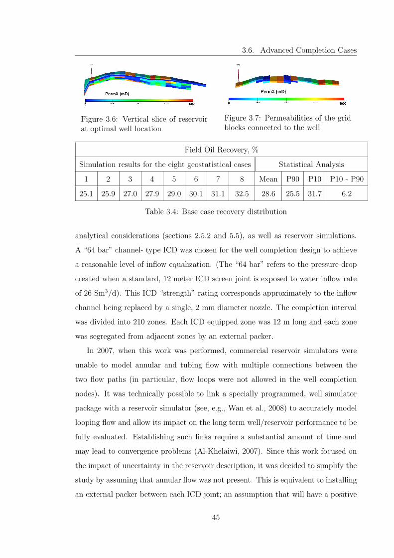
3.6. Advanced Completion Cases
Figure 3.6: Vertical slice of reservoirat optimal well location
Figure 3.7: Permeabilities of the gridblocks connected to the well
Field Oil Recovery, %
Simulation results for the eight geostatistical cases Statistical Analysis
1 2 3 4 5 6 7 8 Mean P90 P10 P10 - P90
25.1 25.9 27.0 27.9 29.0 30.1 31.1 32.5 28.6 25.5 31.7 6.2
Table 3.4: Base case recovery distribution
analytical considerations (sections 2.5.2 and 5.5), as well as reservoir simulations.
A “64 bar” channel- type ICD was chosen for the well completion design to achieve
a reasonable level of inflow equalization. (The “64 bar” refers to the pressure drop
created when a standard, 12 meter ICD screen joint is exposed to water inflow rate
of 26 Sm3/d). This ICD “strength” rating corresponds approximately to the inflow
channel being replaced by a single, 2 mm diameter nozzle. The completion interval
was divided into 210 zones. Each ICD equipped zone was 12 m long and each zone
was segregated from adjacent zones by an external packer.
In 2007, when this work was performed, commercial reservoir simulators were
unable to model annular and tubing flow with multiple connections between the
two flow paths (in particular, flow loops were not allowed in the well completion
nodes). It was technically possible to link a specially programmed, well simulator
package with a reservoir simulator (see, e.g., Wan et al., 2008) to accurately model
looping flow and allow its impact on the long term well/reservoir performance to be
fully evaluated. Establishing such links require a substantial amount of time and
may lead to convergence problems (Al-Khelaiwi, 2007). Since this work focused on
the impact of uncertainty in the reservoir description, it was decided to simplify the
study by assuming that annular flow was not present. This is equivalent to installing
an external packer between each ICD joint; an assumption that will have a positive
45

3.6. Advanced Completion Cases
0.0
2.0
4.0
6.0
8.0
10.0
12.0
14.0
16.0
18.0
19 20 21 22 23 24 25 26 27 28 29 30 31 32 33 34 35 36 37 38 39
Oil Recovery in 30 years, %
Pro
babi
lity
Den
sity
Figure 3.8: Probabilistic production forecast for the Base Case
impact on performance of the ICD completion.
3.6.2 ICV Case
The completion interval was divided into 5 zones, each of which was separately con-
trolled with an infinitely variable, 3 1/2 in. diameter ICV installed in 8 1/2 in. hole.
The well target production rate of 600 Sm3/d was achieved at all times by employ-
ing a similar drawdown for all three completion cases (Figure 3.9 and Table 3.6).
The maximum difference in the flowing bottom hole pressure (FBHP) created at
equivalent stages in the reservoir life by the different completion designs had a value
of 10 bar. The Base Case had the highest FBHP. The FBHP with ICDs installed
was lower than the Base Case due to the imposed, additional pressure drop across
the ICD. The ICV case had the lowest FBHP because, in addition to pressure loss
across the valves, it also has a smaller, flow conduit diameter. The improved ICV
well performance was achieved by limiting the production from zones with a higher
water cut. The weak gas cap had a limited effect. The tested ICV operation policies
that successfully limited gas production also reduced the oil recovery. More sensi-
tive ICV gas cap management strategies might have proved more successful than
author’s attempts.
46

3.7. Results
Figure 3.9: Flowing bottom hole pres-sure comparison for one of the 8 real-isations
Figure 3.10: Recovery comparison forone of the 8 realisations
3.7 Results
Figure 3.10 compares the recovery achieved by the three completion options for the
fourth of the eight geological realisations. It demonstrates that it may be difficult to
tell which completion gives the greatest oil recovery if only a single reservoir model
is employed. Out of the eight reservoir models used here ICDs gave the highest
recovery in 6th, 7th and 8th cases; while the ICVs were most successful in the
remaining 5 cases (Table 3.5).
A probabilistic comparison (Figure 3.11, Table 3.5 and Table 3.6) allows a clearer
comparison of the 30 year oil recovery efficiency of the three alternative completions.
The average predicted recovery for the ICD completion (the green line) was greater
than the corresponding value for the Base Case. However, these two cases show only
minor differences in the uncertainty (the difference between the P10 and the P90
cases) of the recovery forecast at all certainty levels. The ICV completion (red line)
showed both an increased oil recovery as well as delivering a reduction in the uncer-
tainty. Any increase in the oil production was reflected by a corresponding decrease
in the water production since the well production was liquid rate constrained.
47

3.7. Results
Fie
ldO
ilR
ecov
ery,
%
Sim
ula
tion
resu
lts
for
the
eigh
tge
osta
tist
ical
case
sSta
tist
ical
Anal
ysi
s
Cas
e1
23
45
67
8M
ean
P90
P10
P10
-P
90
Bas
e25
.125
.927
.027
.929
.030
.131
.132
.528
.625
.531
.76.
2
“64
Bar
”IC
D27
.027
.928
.729
.630
.431
.432
.233
.430
.127
.432
.75.
3
5IC
Vs
29.0
29.5
29.8
30.1
30.7
31.6
31.7
32.2
30.6
29.1
32.2
3.1
Tab
le3.
5:R
ecov
ery
dis
trib
uti
onfo
rB
ase,
ICD
and
ICV
case
s
48
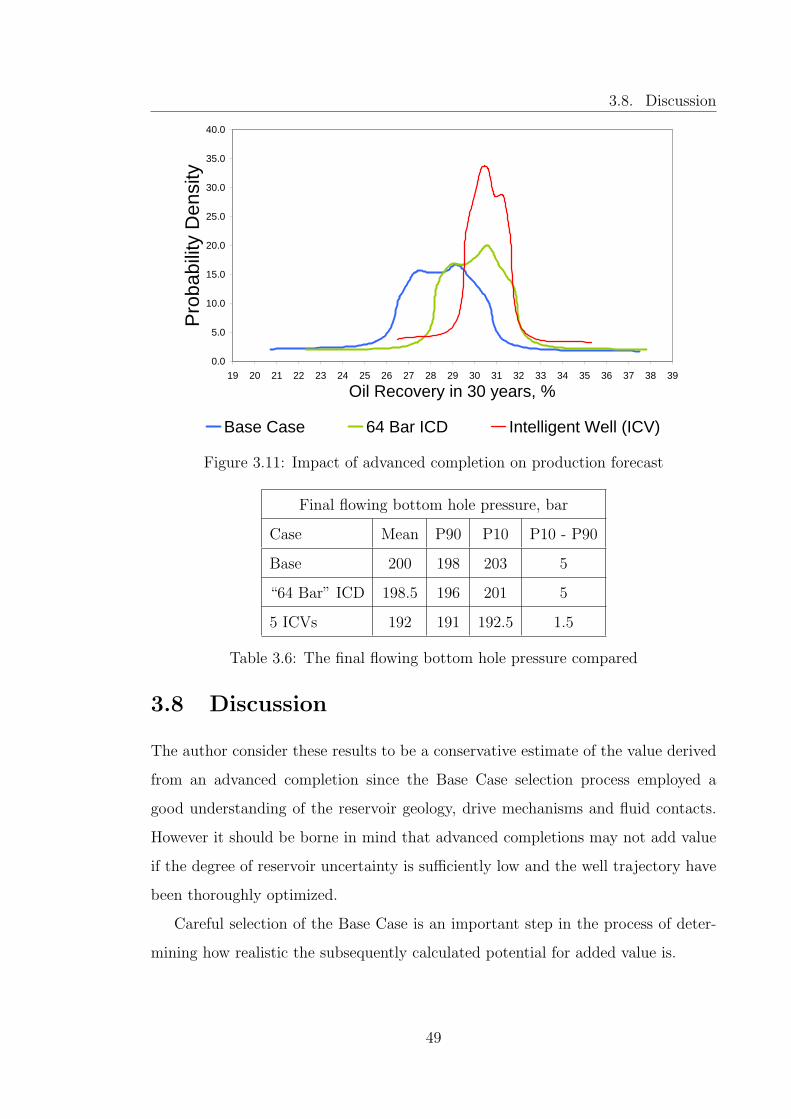
3.8. Discussion
0.0
5.0
10.0
15.0
20.0
25.0
30.0
35.0
40.0
19 20 21 22 23 24 25 26 27 28 29 30 31 32 33 34 35 36 37 38 39
Oil Recovery in 30 years, %
Pro
babi
lity
Den
sity
Base Case 64 Bar ICD Intelligent Well (ICV)
Figure 3.11: Impact of advanced completion on production forecast
Final flowing bottom hole pressure, bar
Case Mean P90 P10 P10 - P90
Base 200 198 203 5
“64 Bar” ICD 198.5 196 201 5
5 ICVs 192 191 192.5 1.5
Table 3.6: The final flowing bottom hole pressure compared
3.8 Discussion
The author consider these results to be a conservative estimate of the value derived
from an advanced completion since the Base Case selection process employed a
good understanding of the reservoir geology, drive mechanisms and fluid contacts.
However it should be borne in mind that advanced completions may not add value
if the degree of reservoir uncertainty is sufficiently low and the well trajectory have
been thoroughly optimized.
Careful selection of the Base Case is an important step in the process of deter-
mining how realistic the subsequently calculated potential for added value is.
49
3.9. Conclusions
3.9 Conclusions
Well completion design has been shown to reduce the impact of geostatistical uncer-
tainty on the production forecast using the uncertainty quantification methodology
as applied in reservoir engineering. The study of the PUNQ-S3 reservoir found that
a well completion designed based on:
• ICDs increased the mean recovery with a limited decrease in of risk.
• ICVs further increased mean recovery and reduced the risk compared to the
base case by 50%.
50
Chapter 4
Impact of Frictional Pressure
Losses Along the Completion on
Well Performance
4.1 Introduction
The impact of frictional pressure losses across the length of completion on well per-
formance is usually negligible for a vertical or deviated well since the well-reservoir
contact length is short, being normally of several tens of meters. Today’s direc-
tional drilling technology allows increased well-reservoir contact, bringing a number
of advantages in terms of the well’s productivity, drainage area and sweep efficiency
together with delay in the breakthrough of water or gas. However, frictional pressure
losses along the completion are an important factor in long, possibly multilateral,
wells. These losses have to be taken into account in order to secure optimum reser-
voir drainage and avoid overestimation of well productivity.
Commercial well and reservoir simulators enable engineers to model this (and
many other complex phenomena) while designing long horizontal and multilateral
wells. In terms of underlying assumptions these products are more general than
analytical models. This allows engineers to quickly consider large number of op-
51

4.2. Literature Review
tions and thus optimise completion design in a timely manner. However, analytical
solutions of fairly complicated situations are still needed to validate the results of
numerical simulators and they often implemented in numerical simulators to provide
the user with an analytical option.
4.2 Literature Review
The first published analysis of the pressure drop along a completion was performed
by Dikken (1990). He used Blasius’s correlation for the turbulent friction factor and
presented solutions for both laminar and turbulent flow cases. The laminar flow
problem was reduced to a linear ordinary differential equation (ODE) of the second
order that has a rigorous closed form solution. Dikken developed analytical formulae
for wells of infinite length for the turbulent flow case and also proposed a numerical
solution for finite wells.
Joshi (1991) suggested a way of assessing the importance of pressure drop along
the completion by assuming that all fluid enters the wellbore at the toe and applying
a standard pipe flow correlation. This simple method largely overestimates the
wellbore pressure drop: dividing Joshi’s result by 3 still gives an upper estimate
(Appendix C). The frictional pressure losses can be neglected if the upper estimate
is small compared to the drawdown. Such calculations have great practical use as
they provide a “quick-look” evaluation to determine whether a more sophisticated
analysis is necessary in any particular case.
Joshi (1991) also considered the ratio of drawdown at the toe and the heel of the
well as one of the key parameters describing the well performance. This parameter
(the drawdown ratio) is designated Rd in this dissertation.
Seines et al. (1993) used Haaland’s flow correlation (Haaland, 1983) and they
noted that, for highly turbulent flow, the friction factor is mainly a function of
the dimensionless wellbore roughness i.e. the dependence of the friction factor on
Reynolds number can be neglected. This allowed reduction of the turbulent flow
52
4.2. Literature Review
problem to the following second order non-linear ODE:
u′′ = u2 (4.1)
where u is normalised well flow rate (Seines et al., 1993).
Eq. (4.1) was solved analytically for the case of infinite wells and numerically for
wells of finite length. The author also introduced characteristic length for horizontal
wells, l∗. The meaning of this parameter will be discussed in subsection 4.6.1 of this
chapter.
Halvorsen (1994) observed that the solution of Eq. (4.1) for finite wells can be
expressed through a Weierstrass elliptic function and expanded into a theta series.
However Halvorsen’s solution still contains an implicit relationship between the ex-
pansion’s parameters which has to be resolved iteratively. The author calculated the
value of q∗w/qinf to eight significant digits (0.96019421). This result was confirmed
by Seines et al. (1993), allowing it to be used as a benchmark for the explicit solution
developed in this thesis.
Landman (1994) extended Dikken’s work by deriving an analytical solution for
turbulent flow in wells of finite length. This solution establishes an implicit relation-
ship between the well rate and the drawdown via use of the Gauss hypergeometric
function. It has to be used iteratively to calculate the well rate for the given draw-
down or vice-versa.
Novy (1995) used Jain’s friction factor correlation (Jain, 1976) and solved the
problem numerically for both liquid and compressible gas flow. He provided guide-
lines as to when friction can be ignored in a particular well.
Ozkan et al. (1995) proposed a quite general dynamic semi-analytical model
that can account for fluid compressibility, various boundary conditions and reser-
voir anisotropy. The model takes the form of a fairly complex non-linear integral
equation. The authors suggest solving it by discretizing in space and time with the
recommendation to use a minimum of 40 well segments. This solution appears to be
similar to the conventional numerical approaches in terms of implementation effort
and computational efficiency.
53

4.2. Literature Review
The semi-analytical model developed by Penmatcha et al. (1999) is mathemat-
ically very similar to that suggested by Seines et al. (1993). Penmatcha’s model is
more complex and potentially more general because it does not employ the:
• Darcy-Weisbach equation.
• Assumption of a constant friction factor.
Penmatcha et al. (1999) introduced a dimensionless variable called productivity
error, Ep , which is the error in the well productivity calculations due to neglecting
frictional pressure drop in the wellbore:
Ep = (qnof − qw) /qnof (4.2)
where qw well flow rate,
qnof well flow rate estimate neglecting friction.
An extensive sensitivity analysis that illustrated the effect of well length, flow rate,
wellbore roughness, reservoir drawdown, fluid viscosity and reservoir permeability
on productivity error was also reported.
Hill and Zhu (2008) suggested an approach similar to that of Joshi (1991). The
main difference is that Hill and Zhu (2008) used half the total flow rate (this is equiv-
alent to dividing the Joshi’s pressure estimate by 4). It is shown in Appendix C that
this approach gives neither an upper nor a lower estimate of the frictional pressure
losses. They did not formally address the question of their method’s precision. It
can not therefore be considered as a rigorous evaluation of well performance.
Many other authors addressed various aspects of frictional pressure losses along
the completion. This review has been restricted to the most relevant works. An ex-
plicit analytical solution for turbulent flow in wellbore has not so far been published.
This chapter presents such a solution based on the same assumptions as those of
previous researchers.
54
4.3. Problem Formulation
4.3 Problem Formulation
Estimation of the two dimensionless variables Rd and Ep (see section 4.2 for defi-
nitions) can give answers to many practical questions related to frictional pressure
losses in a long completion. For instance, the drawdown ratio, Rd, indicates whether
friction skews the inflow profile. A non-uniform inflow profile may decrease oil sweep
efficiency and recovery through a premature water or gas breakthrough. The pro-
ductivity error, Ep, helps to define the well’s inflow performance curve which is one
of the key parameters used in well design.
The motivation for the present work was the development of an explicit analytical
model that would describe turbulent flow in a highly deviated well with a long
completion interval. In particular the model should provide formulae for the:
• Pressure and flow rate profiles along the completion.
• Drawdown ratio Rd.
• Productivity error Ep.
4.3.1 Assumptions
The model invokes the following assumptions with respect to the inflow from the
reservoir. The:
• Well fully penetrates reservoir (or the edge effects due to partial penetration
can be neglected).
• Flow is steady or pseudo-steady state, subject to Darcy’s law.
• Distance between the well and the areal reservoir boundary is much longer
than the well length (or the boundary is parallel to the well).
• Reservoir is homogeneous.
• Perpendicular-to-the-well components of the reservoir pressure gradients are
much greater than the along-hole ones.
55
4.3. Problem Formulation
The above simplifications are required in order to introduce the term of Specific
Productivity Index (PI per unit length) and assume that it is constant throughout
the completion interval. The assumptions about the wellbore flow are that it is:
• Isothermal.
• Incompressible.
• Steady state.
• Homogeneous (no slip between the phases) and the:
• Friction factor is constant along the completion interval.
• Pressure drop due to acceleration is small compared to that of friction.
• Dependence of fluid’s viscosity upon pressure can be neglected.
Note that the completion interval is not assumed to be perfectly horizontal. Under
assumptions stated above, hydrostatic gradient in the reservoir is the same as in
the wellbore what makes the model applicable for deviated wells. There are two
assumptions however that I would like to discuss in more detail.
Constant Friction Factor
The friction factor for highly turbulent flow is determined primarily by the roughness
of the pipe (Figure 4.1). The dependence of its value on Reynolds number is weak.
I chose to neglect this dependency since this allows simplification of the problem
by assuming that the friction factor is constant along the completion interval. In
practice this implies that turbulent flow occupies the majority of the wellbore and
the completion roughness is constant along its length. Appendix A shows how the
average friction factor and the error associated with this averaging can be estimated.
56

4.3. Problem Formulation
0.001
0.01
0.1
1
1.E+02 1.E+03 1.E+04 1.E+05 1.E+06 1.E+07
Reynolds Number
Fann
ing
Fric
tion
Fact
or
Laminar Flow Turbulent, e/D = 0.001Turbulent, e/D = 0.01 Turbulent, e/D = 0.1
Figure 4.1: Fanning friction factor for rough pipes (Haaland’s correlation)
Acceleration
Most authors agree that pressure drop due to acceleration in horizontal wells is
usually small compared to that due to friction. However a quantitative analysis
of conditions, under which the assumption is valid, is not readily available in the
literature. Appendix B shows that acceleration can be ignored if:
faL� D (4.3)
where L length of completion,
D internal diameter of completion,
fa average Fanning friction factor.
This result can be further simplified for wells with predominantly turbulent flow:
long completion intervals with a relatively high roughness (e.g. an open hole or sand
57

4.3. Problem Formulation
screen completion) have a Fanning friction factor with an order of magnitude of 10−2.
The inequality (4.3) can then be transformed into:
L/D > 1000 (4.4)
4.3.2 Mathematical Formulation
Fluid inflow from the reservoir and the pressure drop along the completion interval
are the two interrelated phenomena that this work focuses on. The assumptions
(subsection 4.3.1) allow the inflow to the well to be described as:
dq
dl= j (Pe − P (l)) (4.5)
where q flow rate (in the tubing) at distance l from the toe of the well,
Pe reservoir pressure at the external boundary,
l distance between particular wellbore point and the toe,
j specific productivity index.
The specific productivity index, j, is an empirical parameter indicating that fluid
inflow from reservoir to wellbore is proportional to pressure difference between the
external reservoir boundary and wellbore. It can be estimated with a number of
techniques. For example:
• Analytical PI models (see, e.g., Babu and Odeh, 1989; Goode and Kuchuk,
1991; Goode and Wilkinson, 1991);
• Well log data;
• Well test data.
The Darcy-Weisbach equation that defines the friction factor has the following
form in SI units:dPfdl
= −2f
Dρv2 (4.6)
58

4.3. Problem Formulation
where v is fluid volumetric velocity. Eq. (4.6) can be used for both laminar and
turbulent frictional pressure losses. Note that the Fanning friction factor defined in
(4.6) is four times smaller than the Darcy-Weisbach (Moody) friction factor. The
Fanning friction factor will be referred to in the remainder of the dissertation as the
“friction factor”.
The following form of the Darcy-Weisbach equation (4.6) is more convenient in
the context of the problem under consideration:
dP
dl= −CfρfB
2
D5q2(l) (4.7)
where B formation volume factor,
Cf unit conversion factor: 2.956 · 10−12 in field units and 4.343 · 10−15 in metric.
The system of equations (4.5) and (4.7) can be reduced to a single non-linear
ODE of the second order:d2q
dl2=jCfρfaB
2
D5q2 (4.8)
which is mathematically equivalent to Eq. (4.1). Note that fa was introduced in
Eq. (4.8), an average value of friction factor (Appendix A).
In practice fluid production or injection is controlled either by the target flow
rate or the pressure. Hence the problem may be formulated with one of two sets of
boundary conditions. Flow rate control: q(0) = 0
q(L) = qw(4.9)
or pressure control: q(0) = 0
dq(L)dx
= j∆Pw(4.10)
where Pw flowing bottom hole pressure (at the heel of the tubing) i.e. P (L),
∆Pw the total pressure drop at the heel i.e. Pe − Pw.
59
4.4. Derivation of the Solution
Eq. (4.8), with boundary conditions (4.9) or (4.10), defines the problem to be
solved.
4.4 Derivation of the Solution
4.4.1 General Solution
Let us nondimensionalise Eqs. (4.8)-(4.10). The dimensionless distance from the toe
is:
x = l/L (4.11)
The dimensionless flow rate and the Horizontal Well number for a rate constrained
well (Eq. (4.9)) are:
yq(x) = q(Lx)/qw (4.12)
hq = CfρfB2JsL
2qw/D5 (4.13)
The analogous variables for a pressure constrained well (Eq. (4.10)) are:
yp(x) =q(Lx)
Js∆PwL(4.14)
hp = CfρfB2J2
sL3∆Pw/D
5 (4.15)
Eq. (4.8) may be transformed into
y′′ = hy2 (4.16)
where
h =
hq for a rate constrained well (Eq. (4.9))
hp for a pressure constrained well (Eq. (4.10))(4.17)
60

4.4. Derivation of the Solution
and the boundary conditions correspondingly take the form of: yq(0) = 0
yq(1) = 1(4.18)
or yp(0) = 0
dyp(1)
dx= 1
(4.19)
The drawdown ratio Rd and the productivity error Ep can be expressed directly
through the dimensionless flow rate:
Rd ≡ ∆P (0)/∆P (L) = y′(0)/y′(1) (4.20)
Ep = 1− q(L)
JsL∆P (L)= 1−
(dyq(1)
dx
)−1
= 1− yp(1) (4.21)
Now let us find the general solution of Eq. (4.16). This ODE does not contain
the independent variable x hence its order can be reduced by substitution p = y′
and taking y as a new independent variable:
y′′ ≡ dy′
dx=dy′
dy
dy
dx= p′p (4.22)
Substituting (4.22) into (4.16):
d(p2)/2 = hy2dy (4.23)
p2 = 2hy3/3 + C (4.24)
(y′)2
= 2hy3/3 + C (4.25)
The general solution of (4.25) is expressed through a Weierstrass elliptic function.
Indeed, this function satisfies the differential equation similar to Eq. (4.25):
(℘′)2
= 4℘3 − g2℘− g3 (4.26)
where ℘ (z; g2, g3) is a Weierstrass elliptic function with invariants g2 and g3.
61
4.4. Derivation of the Solution
Comparison of equations (4.25) and (4.26) suggests that in our case g2 = 0.
Let us consider function U(z) = t2℘(tz; 0, g3) where t is an arbitrary number.
One can show that U(z) satisfies the following equation:
(U ′)2
= 4U3 − t6g3 (4.27)
This observation will be used below.
The Weierstrass elliptic function with the parameters g2 = 0, g3 = 1 has the
following properties:
1. It is periodic with half periods of ω1, ω2 and that are related as follows
ω1 = ω2
(1 + i
√3)/2 (4.28)
ω2 = 1.5299540370571934 . . . (4.29)
In particular the points 0, 2ω1, 2ω2 are the vertices of an equilateral triangle.
2. It has a pole of second order at z = 0, and (because it is periodic) at the points
2mω1 + 2nω2 for all integer numbers m, n.
3. ℘(z; 0, 1) equals zero at the centre of that equilateral triangle, namely at the
point
z0 = ω2
(1 + i/
√3)
(4.30)
It also equals zero at the point 2a, and at all the points with coordinates
±a+ 2mω1 + 2nω2 (due to periodicity). Also, it should be borne in mind that
3a = 2ω1 + 2ω2.
We are seeking solution in real values. Hence let us transform ℘(z; 0, 1) into a new
function so that it takes real values on the real line. Using the (4.27) we may take:
R(z) = z20℘(z0 z; 0, 1) (4.31)
This new function (Figure 4.2) has the following properties:
62

4.4. Derivation of the Solution
1. It has real values on the real line.
2. It satisfies the following differential equation: (R′)2 = 4R3 − z60 and hence
R′′ = 6R2.
3. It has a second order pole at points 3n for integer n.
4. It equals zero at points 3n± 1
1 2 3 4 5 6 7z
10
20
30
40
RHzL
Figure 4.2: Plot R(z) = z20℘(z0 z; 0, 1)
Thus R(z) is a particular solution of r′′ = 6r2. Using the observation (4.27) one can
readily write down the corresponding general solution:
r(x) = A2R(Ax+D) (4.32)
Finally, the general solution of (4.16) can be obtained from (4.32) using substitution
y(x) = 6r(x)/h:
y(x) = 6A2R(Ax+D)/h (4.33)
which is equivalent to:
y(x) = 6z20A
2℘ (z0(Ax+D); 0, 1) /h (4.34)
Constant C appearing in (4.25) is linked with A by the following relationship (Us-
nich, 2008):
C =28ω6
2A6
3h2(4.35)
63
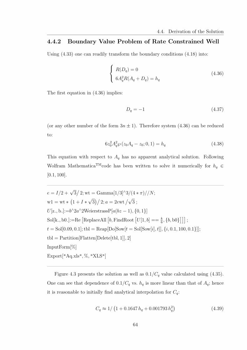
4.4. Derivation of the Solution
4.4.2 Boundary Value Problem of Rate Constrained Well
Using (4.33) one can readily transform the boundary conditions (4.18) into: R(Dq) = 0
6A2qR(Aq +Dq) = hq
(4.36)
The first equation in (4.36) implies:
Dq = −1 (4.37)
(or any other number of the form 3n± 1). Therefore system (4.36) can be reduced
to:
6z20A
2q℘ (z0Aq − z0; 0, 1) = hq (4.38)
This equation with respect to Aq has no apparent analytical solution. Following
Wolfram MathematicaTMcode has been written to solve it numerically for hq ∈
[0.1, 100].
e = I/2 +√
3/
2; wt = Gamma[1/3]∧3/(4 ∗ π)//N ;
w1 = wt ∗(1 + I ∗
√3)/
2; a = 2ewt/√
3 ;
U [z , b ]:=b∧2a∧2WeierstrassP[a(bz − 1), {0, 1}]
Sol[k , b0 ]:=Re[ReplaceAll
[b,FindRoot
[U [1, b] == k
6, {b, b0}
]]];
t = Sol[0.09, 0.1]; tbl = Reap[Do[Sow[t = Sol[Sow[i], t]], {i, 0.1, 100, 0.1}]];
tbl = Partition[Flatten[Delete[tbl, 1]], 2]
InputForm[%]
Export["Aq.xls",%, "XLS"]
Figure 4.3 presents the solution as well as 0.1/Cq value calculated using (4.35).
One can see that dependence of 0.1/Cq vs. hq is more linear than that of Aq; hence
it is reasonable to initially find analytical interpolation for Cq:
Cq ≈ 1/(1 + 0.1647hq + 0.001793h2
q
)(4.39)
64

4.4. Derivation of the Solution
and then use it and Eq. (4.35) to express Aq via hq:
Aq ≈1
ω2
6
√3h2
q
28(1 + 0.1647hq + 0.001793h2
q
) (4.40)
0
0.5
0 5 10 15 20
h q
Aq
0
0.5
0.1/
Cq
Figure 4.3: Numerical solution for Aq
The coefficient of determination (R2) associated with interpolation Eq. (4.39)
is 1.0000. Thus Formula (4.39) can be regarded as precise for most petroleum
engineering applications. Figure 4.4 demonstrates the match between the numerical
solution and its analytical interpolation. Formulae (4.34), (4.37) and (4.40) thus
provide solution to Eq. (4.16) with boundary conditions (4.18).
4.4.3 Boundary Value Problem of Pressure Constrained Well
Eq. (4.25) allows expressing the function through its derivative. Hence the boundary
value problem (4.19) can be reduced in a similar manner to that used previously for
65
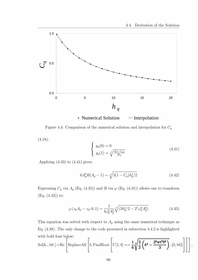
4.4. Derivation of the Solution
0.0
0.5
1.0
0 5 10 15 20
h q
Cq
Numerical Solution Interpolation
Figure 4.4: Comparison of the numerical solution and interpolation for Cq
(4.18): yp(0) = 0
yp(1) = 3
√3(1−Cp)
2hp
(4.41)
Applying (4.33) to (4.41) gives:
6A2pR(Aq − 1) = 3
√3(1− Cp)h2
p/2 (4.42)
Expressing Cp via Aq (Eq. (4.35)) and R via ℘ (Eq. (4.31)) allows one to transform
(Eq. (4.42)) to:
℘ (z0Ap − z0; 0, 1) =1
6z20A
2p
3
√(3h2
p/2− 27ω62A
6p) (4.43)
This equation was solved with respect to Ap using the same numerical technique as
Eq. (4.38). The only change to the code presented in subsection 4.4.2 is highlighted
with bold font below:
Sol[k , b0 ]:=Re
ReplaceAll
b,FindRoot
U [1, b] ==1
63
√3
2
(k2 − 28wt6b6
3
)1
63
√3
2
(k2 − 28wt6b6
3
)1
63
√3
2
(k2 − 28wt6b6
3
), {b, b0}
;
66

4.5. The Solution for Frictional Pressure Losses Along the Completion
The solution was interpolated as follows:
Cp ≈ 1− hp/(1.5 + hp) (4.44)
Ap ≈1
ω2
6
√3h2
p(1− hp/(1.5 + hp))/28 (4.45)
The coefficient of determination (R2) associated with interpolation Eq. (4.44) is
0.9999.
4.5 The Solution for Frictional Pressure Losses
Along the Completion
In section 4.4 the Eqs. (4.8)-(4.10) were nondimensionalised and solved. Now one
can write down the solution in a more practical original dimensional form.
4.5.1 Rate Constrained Well
Solution for a rate constrained well (boundary conditions (4.9)):
∆Pw =qwjL
√2hq/3 + Cq (4.46)
Rd =√Cq/√
2hq/3 + Cq (4.47)
Ep = 1− 1/√
2hq/3 + Cq (4.48)
q(l) = qw6z20A
2q℘ (z0(Aql/L− 1); 0, 1) /hq (4.49)
∆P (l) =qwjL
√2hq (q(l)/qw)3 /3 + Cq (4.50)
where
hq = CfρfaB2jL2qw/D
5 (4.51)
67

4.5. The Solution for Frictional Pressure Losses Along the Completion
Cq ≈(1 + 0.1647hq + 0.001793h2
q
)−1(4.52)
z0 = ω2
(1 + i/
√3)
(4.53)
Aq ≈1
ω2
6
√3h2
q
28(1 + 0.1647hq + 0.001793h2
q
) (4.54)
Horizontal Well number hq can be qualitative interpreted as the ratio of reser-
voir and wellbore conductivity. This number approaches zero when wellbore is much
more conductive then reservoir. Formulae (4.46)-(4.48) give an explicit analytical
solution for the drawdown at the heel ∆Pw, the drawdown ratio Rd and the pro-
ductivity error Ep. Figure 4.5 illustrates Formulae (4.47)-(4.48). One can see, for
example, that:
• Friction reduces well’s productivity by 19% when hq ≈ 1.
• The drawdown at the toe becomes half of that at the heel when hq ≈ 3.
Formula (4.49), describing the flow rate distribution in wellbore, employs a spe-
cial function ℘ called the Weierstrass elliptic function (Abramowitz and Stegun,
1965, Ch. 18). Algorithms for calculating this function are available in literature
(see, e.g., Eckhardt, 1980; Coquereaux et al., 1990; Baker, 1992). It can also be com-
puted using specialised mathematical software (Maplesoft, 2009; Wolfram, 2009).
Formula (4.52) is, strictly speaking, an interpolation of a numerical solution
(subsection 4.4.2). However, the high precision of this interpolation allows one to
regard formula (4.52) as being precise since the maximum discrepancy associated
with the interpolation is less than 0.2% for hq ≤ 10. The interpolation remains
robust even for much higher values of hq with the maximum discrepancy being
about 2% for hq ≤ 100. I believe that scenario of hq > 10 is of little practical
interest since it corresponds to a productivity error Ep > 60% and a drawdown
ratio Rd < 23%.
68
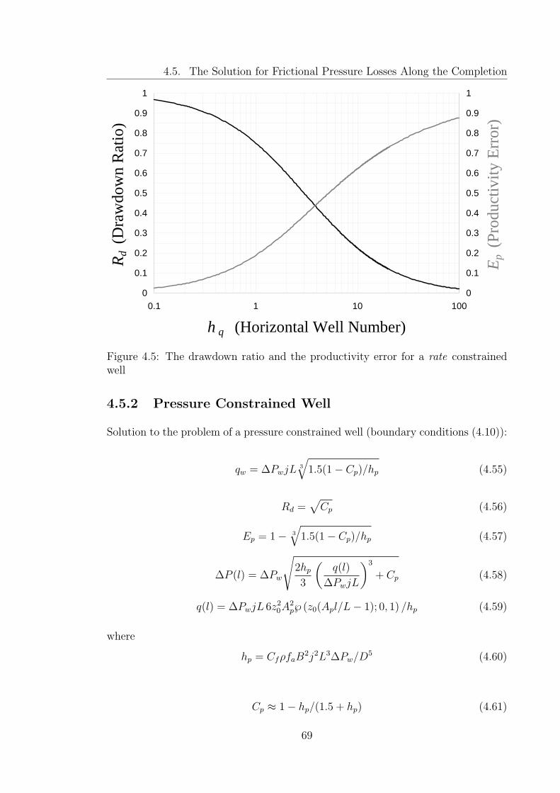
4.5. The Solution for Frictional Pressure Losses Along the Completion
0
0.1
0.2
0.3
0.4
0.5
0.6
0.7
0.8
0.9
1
0.1 1 10 100
h q (Horizontal Well Number)
Rd
(D
raw
dow
n R
atio
)
0
0.1
0.2
0.3
0.4
0.5
0.6
0.7
0.8
0.9
1
Ep
(Pr
oduc
tivity
Err
or)
Figure 4.5: The drawdown ratio and the productivity error for a rate constrainedwell
4.5.2 Pressure Constrained Well
Solution to the problem of a pressure constrained well (boundary conditions (4.10)):
qw = ∆PwjL3
√1.5(1− Cp)/hp (4.55)
Rd =√Cp (4.56)
Ep = 1− 3
√1.5(1− Cp)/hp (4.57)
∆P (l) = ∆Pw
√2hp3
(q(l)
∆PwjL
)3
+ Cp (4.58)
q(l) = ∆PwjL 6z20A
2p℘ (z0(Apl/L− 1); 0, 1) /hp (4.59)
where
hp = CfρfaB2j2L3∆Pw/D
5 (4.60)
Cp ≈ 1− hp/(1.5 + hp) (4.61)
69

4.5. The Solution for Frictional Pressure Losses Along the Completion
Ap ≈1
ω2
6
√3h2
p(1− hp/(1.5 + hp))/28 (4.62)
Formula (4.61) is less accurate than its analogue (4.52) for the rate constrained
well since the author was unable to find a better interpolation for Cp. The average
mismatch between precise numerical solution and its interpolation is about 3% for
hp ≤ 20 (Table 4.1). The horizontal well number hp does not normally exceed
20 in practical well designs. However the approximation still gives sensible results
for values of hp well above 20. E.g. the maximum mismatch is about 20% for
hp ≤ 50. Figure 4.6 presents the precise solution for the drawdown ratio Rd and the
productivity error Ep. The table of precise values of Cp is available in Excel format
as supplementary data of this dissertation.
0
0.1
0.2
0.3
0.4
0.5
0.6
0.7
0.8
0.9
1
0.1 1 10 100
h p (Horizontal Well Number)
Rd
(D
raw
dow
n R
atio
)
0
0.1
0.2
0.3
0.4
0.5
0.6
0.7
0.8
0.9
1
Ep
(Pr
oduc
tivity
Err
or)
Figure 4.6: The drawdown ratio and the productivity error for a pressure constrainedwell
The relative simplicity of formula (4.61) allows one to conveniently express the
70
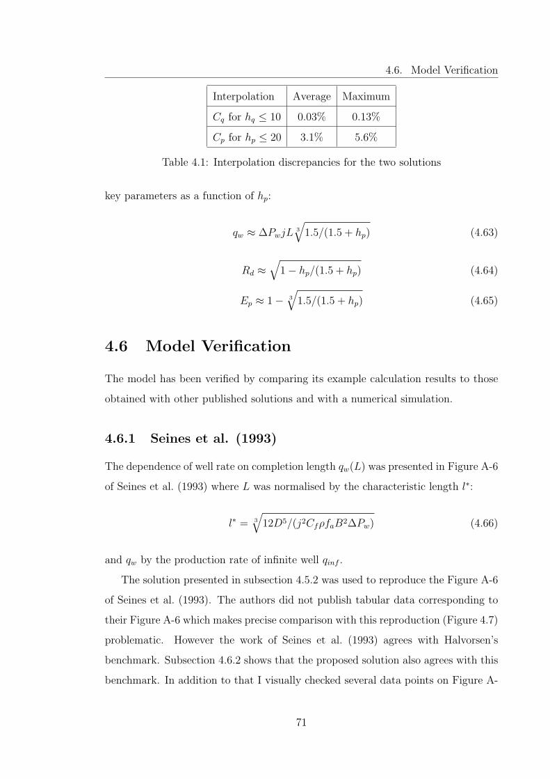
4.6. Model Verification
Interpolation Average Maximum
Cq for hq ≤ 10 0.03% 0.13%
Cp for hp ≤ 20 3.1% 5.6%
Table 4.1: Interpolation discrepancies for the two solutions
key parameters as a function of hp:
qw ≈ ∆PwjL3
√1.5/(1.5 + hp) (4.63)
Rd ≈√
1− hp/(1.5 + hp) (4.64)
Ep ≈ 1− 3
√1.5/(1.5 + hp) (4.65)
4.6 Model Verification
The model has been verified by comparing its example calculation results to those
obtained with other published solutions and with a numerical simulation.
4.6.1 Seines et al. (1993)
The dependence of well rate on completion length qw(L) was presented in Figure A-6
of Seines et al. (1993) where L was normalised by the characteristic length l∗:
l∗ = 3
√12D5/(j2CfρfaB2∆Pw) (4.66)
and qw by the production rate of infinite well qinf .
The solution presented in subsection 4.5.2 was used to reproduce the Figure A-6
of Seines et al. (1993). The authors did not publish tabular data corresponding to
their Figure A-6 which makes precise comparison with this reproduction (Figure 4.7)
problematic. However the work of Seines et al. (1993) agrees with Halvorsen’s
benchmark. Subsection 4.6.2 shows that the proposed solution also agrees with this
benchmark. In addition to that I visually checked several data points on Figure A-
71

4.6. Model Verification
6 of Seines et al. (1993) and confirmed that they match the results given by the
proposed solution. For example, L/l∗ of 0.322 corresponds to qw/qinf of 0.591. On
this basis, I believe that presented solution is consistent with the results of Seines
et al. (1993).
The authors classified their characteristic length as being “optimal” because if:
• L = l∗, the well’s production rate is almost identical to that of infinite length
well (q∗w ≈ qinf );
• L < l∗, then the well’s production rate decreases rapidly with decreasing L;
• L > l∗, then the production rate increases only marginally with increasing L
(Seines et al., 1993).
0
0.5
1
0 0.5 1
L/ l *
q w /q
inf
Figure 4.7: The dependence of well rate on completion length
Seines et al. (1993) used logarithmic scale for their Figure A-6. This may create
the erroneous impression that the function qw(L) changes its curvature from concave
up at small L to concave down at large L. In fact, it is concave down for all positive
L (see Figure 4.7 with its linear scale). This is as expected from the basic physics:
72

4.6. Model Verification
the production gain from every extra metre extension to the completion interval is
smaller than that from the previous one (due to frictional pressure losses).
I could not ascribe any specific mathematical significance to the point L = l∗
of function qw(L). I believe that in order to define a practical optimal completion
length one has to broaden the definition of the problem itself, e.g. involve economical,
reservoir and (or) risk analysis.
4.6.2 Halvorsen (1994)
According to Halvorsen (1994), a well of l∗ length produces 96% of the production
rate of an infinite well (more precisely q∗w/qinf = 0.96019421). The proposed explicit
analytical solution gives 0.961 (Appendix D); a difference of 0.08% from Halvorsen’s
result. This minor discrepancy is due to the interpolation used to represent the
solution explicitly. The precision can be further improved by use of look-up tables
or more sophisticated interpolation techniques. However these approaches are con-
sidered unnecessary since the errors associated with model’s assumptions and the
uncertainty associated with the input parameters are, in practice, much higher than
this mathematical error.
The drawdown ratio for a such well is 0.34, i.e. the inflow rate at the toe is only
one third of that at the heel. This difference may affect reservoir sweep efficiency.
4.6.3 Penmatcha et al. (1999)
The example well case considered by Penmatcha et al. (1999) was used to compare
his model to that presented in section 4.5. Table 4.2 outlines Penmatcha’s parame-
ters. According to my calculations, the average Fanning friction factor in this case
is 0.0048 and the horizontal well number hq equals 16.5. The mismatch in the draw-
down estimates given by the two models (Table 4.3) is 10%. The mismatch in the
productivity error is less than 5%. Unfortunately the level of detail provided by
Penmatcha et al. (1999) was insufficient to allow me to identify the exact cause of
these mismatches. The results of numerical simulation performed using commercial
well modelling software (Weatherford, 2008) lie between Penmatcha’s results and
73
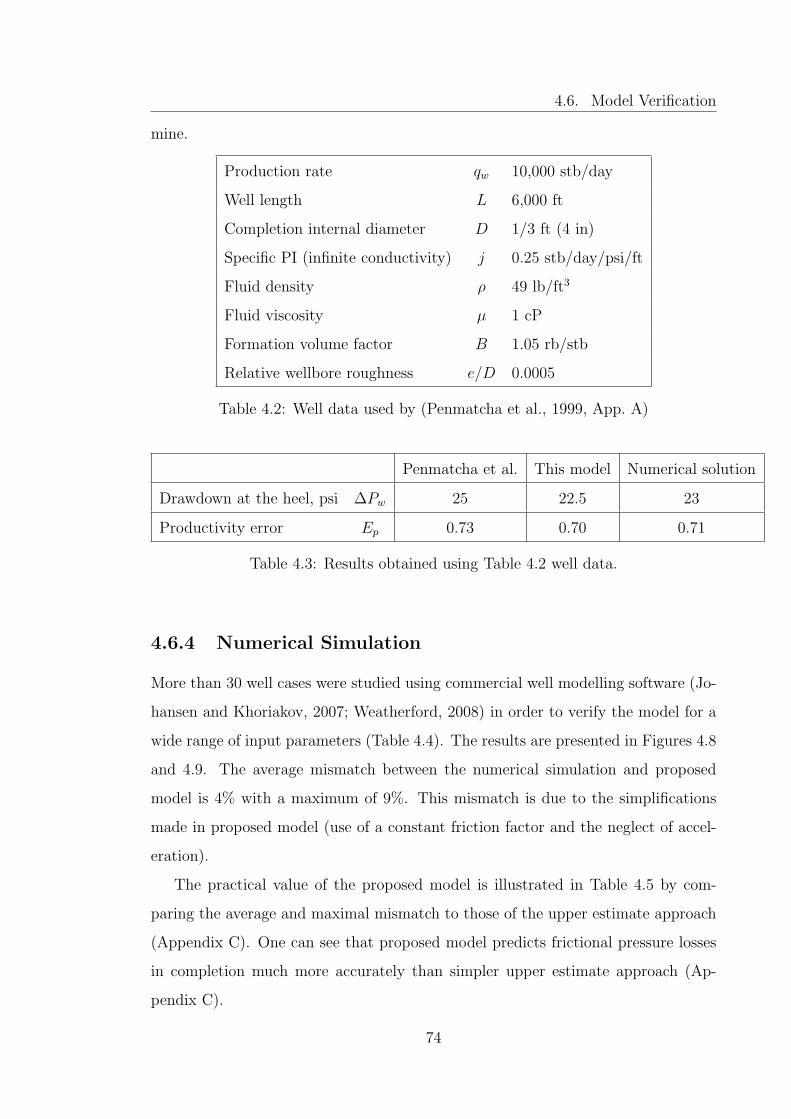
4.6. Model Verification
mine.
Production rate qw 10,000 stb/day
Well length L 6,000 ft
Completion internal diameter D 1/3 ft (4 in)
Specific PI (infinite conductivity) j 0.25 stb/day/psi/ft
Fluid density ρ 49 lb/ft3
Fluid viscosity µ 1 cP
Formation volume factor B 1.05 rb/stb
Relative wellbore roughness e/D 0.0005
Table 4.2: Well data used by (Penmatcha et al., 1999, App. A)
Penmatcha et al. This model Numerical solution
Drawdown at the heel, psi ∆Pw 25 22.5 23
Productivity error Ep 0.73 0.70 0.71
Table 4.3: Results obtained using Table 4.2 well data.
4.6.4 Numerical Simulation
More than 30 well cases were studied using commercial well modelling software (Jo-
hansen and Khoriakov, 2007; Weatherford, 2008) in order to verify the model for a
wide range of input parameters (Table 4.4). The results are presented in Figures 4.8
and 4.9. The average mismatch between the numerical simulation and proposed
model is 4% with a maximum of 9%. This mismatch is due to the simplifications
made in proposed model (use of a constant friction factor and the neglect of accel-
eration).
The practical value of the proposed model is illustrated in Table 4.5 by com-
paring the average and maximal mismatch to those of the upper estimate approach
(Appendix C). One can see that proposed model predicts frictional pressure losses
in completion much more accurately than simpler upper estimate approach (Ap-
pendix C).
74

4.7. Discussion
0.0
0.5
1.0
0 5 10 15 20
h q
Rd
Numerical Solution Our Analytical Solution
Figure 4.8: Numerical verification of Eq. (4.47) for the drawdown ratio, Rd, in arate constrained well.
4.7 Discussion
The proposed closed form solution for turbulent frictional pressure drop along com-
pletions fills in the gap between the established analytical models that neglect this
phenomenon and the numerical simulators that allow its detailed analysis. The
dimensionless numbers used in the model introduce a succinct and comprehensive
terminology for description of frictional pressure drop effects in horizontal wells.
Implementation of the solution is straightforward. It can be incorporated into
engineering spreadsheets and used for applications such as:
• Identifying well design where the frictional pressure drop along the comple-
tion’s length warps the inflow profile. Such wells are likely to benefit from ICD
installation.
• Scoping economic analysis of the optimal well diameter and length.
Presented model is computationally efficient due to its explicit form. This makes
it the preferred choice for use in computationally expensive applications such as
75
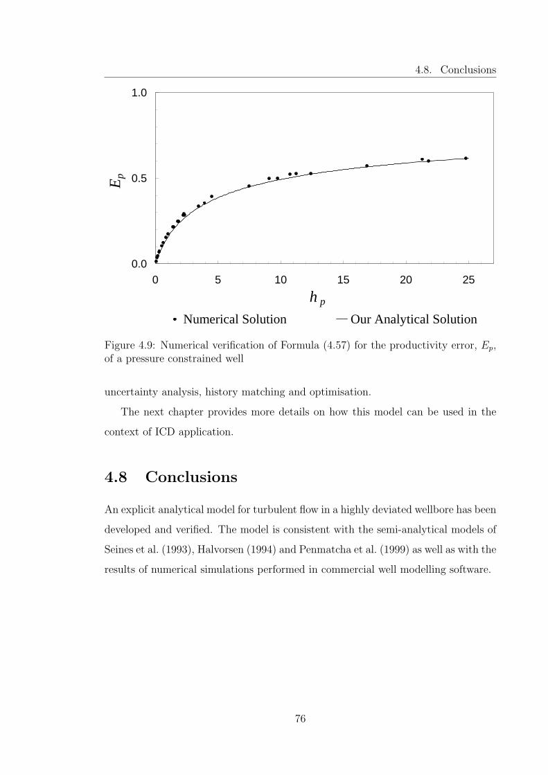
4.8. Conclusions
0.0
0.5
1.0
0 5 10 15 20 25
h p
Ep
Numerical Solution Our Analytical Solution
Figure 4.9: Numerical verification of Formula (4.57) for the productivity error, Ep,of a pressure constrained well
uncertainty analysis, history matching and optimisation.
The next chapter provides more details on how this model can be used in the
context of ICD application.
4.8 Conclusions
An explicit analytical model for turbulent flow in a highly deviated wellbore has been
developed and verified. The model is consistent with the semi-analytical models of
Seines et al. (1993), Halvorsen (1994) and Penmatcha et al. (1999) as well as with the
results of numerical simulations performed in commercial well modelling software.
76

4.8. Conclusions
Parameter Minimum Maximum
L Well length, ft 2 000 17 000
D Completion internal diameter, in 4 8.5
j Specific PI, STB/day/psi/ft 0.003 0.78
ρ Fluid density, lb/ft3 43 53
µ Fluid viscosity, cP 0.7 12
∆Pw Drawdown at the heel, psi 1.1 450
qw Production rate, STB/day 150 13 000
Reh Reynolds number at the heel 4 · 103 3 ·105
Table 4.4: Range of parameters studied during the numerical verification process(subsection 4.6.4)
Average Maximum
Main model (section 4.5) 4% 9%
Upper estimate (Appendix C) 20% 60%
Table 4.5: Pressure mismatch with numerical simulation
77
Chapter 5
Reduction of the Horizontal Well’s
Heel-Toe Effect with Inflow
Control Devices
5.1 Introduction
Increasing well-reservoir contact has a number of potential advantages in terms of
well productivity, drainage area, sweep efficiency and delayed water or gas break-
through. However, long, possibly multilateral, wells not only bring advantages, but
also present new challenges in terms of drilling, completion and production. One
of these challenges is the frictional pressure losses increasing with well length. The
inflow profile becomes distorted so that the heel part of the well produces more
fluid than the toe when these losses become comparable to drawdown. This inflow
imbalance, in turn, often causes premature water or gas breakthrough. It should
thus be avoided.
Installation of Inflow Control Devices (ICDs) is an advanced well completion
option that provides a practical solution to this challenge. An ICD is a well com-
pletion device that directs the fluid flow from the annulus into the base pipe via a
flow restriction. This restriction can be in form of channels (Figure 1.2), nozzles or
78

5.1. Introduction
orifices (Figure 1.3). In all cases the ability of an ICD to equalise the inflow along
the well length is due to the difference in the physical laws governing fluid flow in
the reservoir and through the ICD. Liquid flow in porous media is normally laminar,
hence there is a linear relationship between the flow velocity and the pressure drop.
By contrast, the flow regime through an ICD is turbulent, resulting in a quadratic
velocity/pressure drop relationship.
The physical laws of flow through an ICD make it especially effective in reducing
the free gas production. In-situ gas viscosity under typical reservoir conditions is
normally at least an order of magnitude lower than that of oil or water; while in-situ
gas density is only several times smaller than that of oil or water. Gas inflow into
a well will thus dominate after the initial gas breakthrough if it is not restricted by
gravity (Mjaavatten et al., 2008) or an advanced completion. ICDs introduce an
extra pressure drop that is proportional to the square of the volumetric flow rate.
The dependence of this pressure drop on fluid viscosity is weak for channel devices
and totally absent if nozzle or orifice ICDs are used. These characteristics enable
ICDs to effectively reduce high velocity gas inflow.
The magnitude of a particular ICD’s resistance to flow depends on the dimensions
of the installed nozzles or channels. This resistance is often referred to as the ICD’s
“strength”. It is set at the time of installation and can not be changed without a
major intervention to recomplete the well.
ICDs have been installed in hundreds of wells during the last decade, being now
considered to be a mature, well completion technology. Steady-state performance of
ICDs can be analysed in detail with well modelling software (Ouyang and Huang,
2005; Johansen and Khoriakov, 2007). Most reservoir simulators include basic func-
tionality for ICD modelling. Some of them (Wan et al., 2008; Neylon et al., 2009)
also offer practical means of capturing the effects of annular flow. Thus, current
numerical simulation software enables engineers to properly perform the design and
economic justification of an ICD completion. However relatively simple analytical
models still have a role in:
• Quick feasibility studies (screening ICD installation candidates).
79
5.2. Assumptions
• Verification of numerical simulation results.
• Communicating best practices in a non-product specific manner.
This chapter proposes analytical and numerical solutions to the problem of re-
ducing the heel-toe effect with ICDs. These solutions allows one to estimate the:
• ICD design parameters that reduce the heel-toe effect to the required level.
• Impact of ICD on the well’s inflow peformance relationship (IPR).
5.2 Assumptions
The reservoir inflow model employed assumptions that:
• Flow is steady or pseudo-steady state and is described by Darcy’s law.
• The distance between the well and the areal reservoir boundary is much longer
than the well length (or the boundary is parallel to the well).
• The reservoir is homogeneous.
• Edge effects (due to semi radial inflow at the heel and the toe) are negligible.
• The perpendicular-to-the-well components of the reservoir pressure gradients
are much greater than the along-hole ones.
The above simplifications are fairly typical for other analytical solutions that
couple reservoir and wellbore flow using a specific productivity index (section 4.2).
In the model presented in this chapter a specific productivity index, j, is assumed
to be constant throughout the completion interval and equal to the ratio of well’s
Productivity Index (J) and the completion length (L):
j = J/L (5.1)
80

5.2. Assumptions
Generally speaking, j is an empirical parameter that implies fluid inflow from the
reservoir to wellbore is proportional to the pressure difference between the external
reservoir boundary and the annulus:
dq
dl= j(l)(Pe − Pa(l)) (5.2)
Eq. (5.2) is a repeat of Eq. (4.5) after rewriting in a notation more suited for this
chapter.
The flow along the wellbore is assumed to be:
• Isothermal.
• Incompressible.
• Steady state.
• Homogeneous (no slip between the phases)
and the:
• Friction factor is constant along the completion interval.
• Pressure drop due to acceleration is small compared to that of friction.
• Dependence of fluid’s viscosity upon pressure can be neglected.
Note that the completion interval is not assumed to be perfectly horizontal: True
Vertical Depth (TVD) can vary along the completion since the reservoir pressure at
the external boundary Pe is measured at the same TVD as the corresponding point
l of the tubing.
Figure 1.2 and Figure 1.3 illustrate a typical ICD. The assumptions made about
flow within ICD will now be described in more detail:
1. There is no flow in the annulus parallel to the base pipe i.e. fluid flows from
reservoir directly into the ICD’s screen. This assumption is reasonable when:
• ICDs are combined with a number of intermediate packers or a gravel
pack (Augustine et al., 2008) or
81

5.3. Problem Formulation
• The wellbore has collapsed around the screen so that annular flow is no
longer possible.
2. ICDs of the same design (or “strength” of pressure drop) are installed through-
out the completion length. This is the most common type of ICD application
due to the relative simplicity of its design and installation (Henriksen et al.,
2006). Variable “strength” ICD completions have been reported (Helmy et al.,
2006; McIntyre et al., 2006), but they require a more complex design based on
a detailed and reliable description of j along the wellbore at the time of com-
pletion installation in addition to increased operational risk of not installing
them at the correct depth.
3. The flow distribution along the wellbore’s internal flow conduit q(l) is “smooth”
(i.e. has a continuous derivative). Strictly speaking, this distribution is step-
like because fluid enters wellbore through a number of point-like sources (ICD’s
nozzles or channels). However these steps are relatively small if the number of
sources (or ICD completion joints of approximately 12 m length) is sufficiently
large (e.g. > 50). This assumption is usually valid as a typical ICD well com-
pletion has more than 100 ICD joints. This assumption was introduced since
dealing with continuous variables is mathematically more convenient.
5.3 Problem Formulation
5.3.1 General Formulation
Let us consider fluid flow through an ICD joint in order to obtain a mathematical
formulation of the problem. The total pressure difference between the reservoir and
the base pipe (tubing), ∆P , can be divided into the pressure drop in the reservoir,
∆Pr, and the pressure drop in ICD, ∆PICD:
∆P = ∆Pr + ∆PICD (5.3)
82

5.3. Problem Formulation
In terms of mathematics, the inflow is the derivative of flow rate with respect to the
measured depth. A separate notation U is designate to it here since it will be used
extensively in this and next chapters:
U(l) ≡ dq(l)
dl(5.4)
Then one can rewrite (5.2) as:
∆Pr(l) = U(l)/j (5.5)
The pressure drop generated by an ICD is proportional to the second power of
the flow rate through the ICD (Schlumberger, 2009). In terms of specific inflow it
is:
∆PICD = aU2(l) (5.6)
where
a =
(ρcal µρµcal
)1/4ρρcal
l2ICDB2aICD for channel ICDs
Cuρl2ICDB2
C2dd
4 for nozzle or orifice ICDs
(5.7)
The effective nozzle or orifice diameter, d, and the channel ICD rating, aICD,
determine the pressure drop across the appropriate type of ICD. The industrial
“bar” rating (Table 5.1) refers to the pressure drop created when a standard, 12
meter long ICD joint is exposed to a water flow rate of 26 Sm3/d (Henriksen et al.,
2006). It is used as a convenient method of comparing the pressure drop achieved
by different types of ICDs.
Industrial “bar” rating 0.2 0.4 0.8 1.6 3.2
aICD, bar/(Rm3/day)2 0.00028 0.00055 0.00095 0.0016 0.0032
aICD, psi/(Rbbl/day)2 0.00076 0.0015 0.0026 0.0044 0.0087
Table 5.1: Channel ICD strength
83

5.3. Problem Formulation
Substitution of equation (5.5) and (5.6) into (5.3) gives a quadratic equation
with respect to the specific flow rate through the ICD completion:
∆P (l) = aU2(l) + U(l)/j(l) (5.8)
Eq. (5.8) has two real roots. The negative root has no physical meaning since the
inflow rate must be positive as long as reservoir pressure, Pe, is greater than pressure
in the base pipe P . Thus, the solution of Eq. (5.8) is:
U(l) =−1 +
√1 + 4a∆P (l)j2(l)
2aj(l)(5.9)
The well production rate, qw, is the integral of (5.9) over the well length:
qw =
∫ L
0
−1 +√
1 + 4a∆P (l)j2(l)
2aj(l)dl (5.10)
Formulae (5.9) and (5.10) are quite general as they account for both reservoir
heterogeneity and frictional pressure losses in the base pipe. However, these formulae
alone are of little practical utility without information or assumptions on pressure,
∆P (l), and specific productivity index, j(l). The next section presents a practical
formulation of the problem for the case when j can be treated as a constant (Eq. 5.1).
5.3.2 Formulation for a Homogeneous Reservoir
An explicit analytical model for the turbulent frictional pressure losses along a con-
ventional well completion was presented in Chapter 4. The governing equations for
this case are (4.5) and (4.7). They can be reduced to a single non-linear ODE of
the second order which was solved in section 4.4.
Eq. (4.5) should be substituted with Eq. (5.8) when Inflow Control Devices are
applied. This can then be rewritten as:
a
(dq
dl
)2
+1
j
dq
dl= (Pe − P (l)) (5.11)
84
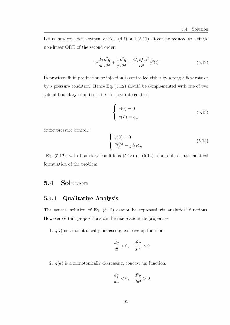
5.4. Solution
Let us now consider a system of Eqs. (4.7) and (5.11). It can be reduced to a single
non-linear ODE of the second order:
2adq
dl
d2q
dl2+
1
j
d2q
dl2=CfρfB
2
D5q2(l) (5.12)
In practice, fluid production or injection is controlled either by a target flow rate or
by a pressure condition. Hence Eq. (5.12) should be complemented with one of two
sets of boundary conditions, i.e. for flow rate control: q(0) = 0
q(L) = qw(5.13)
or for pressure control: q(0) = 0
dq(L)dl
= j∆Prh(5.14)
Eq. (5.12), with boundary conditions (5.13) or (5.14) represents a mathematical
formulation of the problem.
5.4 Solution
5.4.1 Qualitative Analysis
The general solution of Eq. (5.12) cannot be expressed via analytical functions.
However certain propositions can be made about its properties:
1. q(l) is a monotonically increasing, concave-up function:
dq
dl> 0,
d2q
dl2> 0
2. q(a) is a monotonically decreasing, concave up function:
dq
da< 0,
d2q
da2> 0
85
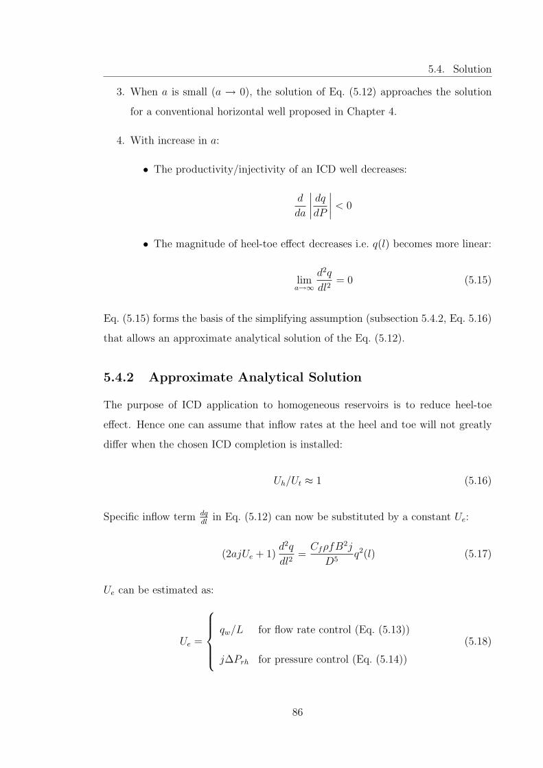
5.4. Solution
3. When a is small (a → 0), the solution of Eq. (5.12) approaches the solution
for a conventional horizontal well proposed in Chapter 4.
4. With increase in a:
• The productivity/injectivity of an ICD well decreases:
d
da
∣∣∣∣ dqdP∣∣∣∣ < 0
• The magnitude of heel-toe effect decreases i.e. q(l) becomes more linear:
lima→∞
d2q
dl2= 0 (5.15)
Eq. (5.15) forms the basis of the simplifying assumption (subsection 5.4.2, Eq. 5.16)
that allows an approximate analytical solution of the Eq. (5.12).
5.4.2 Approximate Analytical Solution
The purpose of ICD application to homogeneous reservoirs is to reduce heel-toe
effect. Hence one can assume that inflow rates at the heel and toe will not greatly
differ when the chosen ICD completion is installed:
Uh/Ut ≈ 1 (5.16)
Specific inflow term dqdl
in Eq. (5.12) can now be substituted by a constant Ue:
(2ajUe + 1)d2q
dl2=CfρfB
2j
D5q2(l) (5.17)
Ue can be estimated as:
Ue =
qw/L for flow rate control (Eq. (5.13))
j∆Prh for pressure control (Eq. (5.14))
(5.18)
86

5.4. Solution
Eq. (5.17) is mathematically equivalent to Eq. (4.8) which was solved in Chap-
ter 4; allowing solutions for a rate and pressure constrained wells as follows.
Rate Constrained Well
The solution for a rate constrained well (boundary conditions (5.13)) is:
U(l) ≈ qwL
√2iq (l/L)3 /3 +Gq (5.19)
Ut ≡ U(0) ≈ qw√Gq/L (5.20)
Uh ≡ U(L) ≈ qwL
√2iq/3 +Gq (5.21)
∆Pw = aU2h + Uh/j (5.22)
where
iq =CfρfaB
2jL2qw(2ajqw/L+ 1)D5
(5.23)
Gq ≈(1 + 0.1647 iq + 0.001793 i2q
)−1(5.24)
Pressure Constrained Well
The solution to the problem of a pressure constrained well (boundary conditions
(5.14)) is:
qw ≈ J∆Prh3
√1.5/(1.5 + ip) (5.25)
U(l) ≈ j∆Prh
√(1−Gp) (l/L)3 +Gp (5.26)
Ut ≡ U(0) ≈ j∆Prh√Gp (5.27)
Uh ≡ U(L) = j∆Prh (5.28)
where
ip =CfρfaB
2j2L3∆Prh(2aj2∆Prh + 1)D5
(5.29)
87

5.5. Choosing an Appropriate ICD Strength
Gp ≈ 1− ip/(1.5 + ip) (5.30)
5.4.3 Numerical Solution
I implemented a numerical solution of Eq. (5.12) using the shooting method with
the starting boundary condition:
dq(0)
dl= Ue (5.31)
where Ue is given by formula (5.18).
The corresponding Wolfram MathematicaTMcode is:
sol = NDSolve[{2ny”[x]y′[x] + y”[x] == hy[x]∧2, y[0] == 0, y′[1] == 1}, y, x,
Method → {"Shooting", "StartingInitialConditions" → {y[0] == 0, y′[0] ==
1}}];
Section 5.6 compares the results of my numerical solution to those obtained
with the most appropriate of the commercial well modelling software (Johansen and
Khoriakov, 2007; Halliburton, 2009).
5.5 Choosing an Appropriate ICD Strength
An increase in the strength of an ICD will improve the inflow equalisation while at
the same time leading to a reduction in the well’s Inflow Performance Relationship
(IPR). The trade-off between reducing well productivity and the increasing degree
of inflow equalisation is the key issue in ICD technology application. One can choose
an ICD strength value that gives a reasonable compromise between the inflow per-
formance and the inflow equalisation by using either the analytical or the numerical
solution of Eq. (5.12) or commercial well modelling software. In this section I present
88

5.5. Choosing an Appropriate ICD Strength
another analytical way of choosing ICD strength which is simpler but less rigorous
than above mentioned methods.
Production from horizontal well is often constrained by the requirement that the
drawdown at the heel should be small enough to avoid premature breakthrough of
water or gas. Proposed analytical approach to the choice of the appropriate ICD
strength is based on the supposition that the ICD should introduce an additional
pressure drop of the same order of magnitude as the reservoir drawdown (Table 2.5).
This translates, in context of the heel-toe effect, to the requirement that the pressure
drop across the ICD should be of the same order of magnitude as the drawdown at
the heel ∆Prh:
∆PICD ≈ n∆Prh (5.32)
where n is a positive dimensionless number (see Eq. 5.36).
The ICD strength required to produce such a pressure drop is obtained from
Eqs. (5.5) and (5.6):
a ≈ nL2
∆PrhJ2(5.33)
Eq. (5.33) can take two forms depending on the type of flow restriction installed in
the ICD (Eq. (5.7)). For a
1. Channel type of ICD:
aICD ≈(ρ µcalρcal µ
)1/4ρcal nL
2
ρ l2ICDB2∆PrhJ2
(5.34)
2. Nozzle/orifice ICDs:
d ≈(Cuρl
2ICDB
2∆PrhJ2
C2dnL
2
)1/4
(5.35)
The higher values of n correspond to a greater ICD “strength” and hence a smaller
difference between the heel and toe specific inflows. I suggest the following “rule of
thumb” for choosing n (and hence the ICD “strength”):
n ≈ (Uh/Ut)noICD − 1 (5.36)
89
5.6. Case Study
where (Uh/Ut)noICD is the ratio of inflow at the heel and at the toe for an equivalent
conventional (no ICD) well produced with the same drawdown at the heel. This
ratio can be estimated with well modelling software or analytical model presented
in section 4.5.
In author’s opinion the pressure interaction between the reservoir and the ICD
is the key factor for solving the problem of selecting the appropriate ICD strength.
However, it should be borne in mind that this problem has no general or “correct”
solution. The preferred solution will also be influenced by factors beyond the scope
of this simple analysis (e.g. economics, field development strategy, annulus flow,
gas production, clean-up, erosion etc.) which are only relevant to a specific field
application.
5.6 Case Study
ICDs were invented by Norsk Hydro for use in the Troll field, one of the Norwegian
continental shelf’s largest oil and gas producing fields (Henriksen et al., 2006). The
thin oil column (4 - 27 m) present across much of the field represented a tremendous
challenge, both in terms of drilling and completion operations, due to the require-
ment to produce oil prior to large scale gas production from the gas cap. Only the
thickest part of oil column was initially recognised as proven reserves, despite the
large volume of oil in place in the part of the field with a thinner column. However,
the construction of wells with increasingly longer horizontal sections, the implemen-
tation of multilateral well technology and the application of ICDs during the last
decade have resulted in the successful development of an increasing fraction of the
oil volume originally-in-place.
The Troll reservoir, a permeable homogeneous sandstone, is thus an ideal candi-
date for illustrating the practical utility of the proposed analytical solution for ho-
mogeneous reservoirs (see Table 5.2 for Troll field data). Being an oil rim reservoir,
the Troll field has the initial reservoir pressure equal to the bubble point pressure.
Strictly speaking, one should use Vogel’s (non-linear) formula to calculate the inflow
performance for this reservoir. However, the difference between a linear and a Vogel
90

5.6. Case Study
IPR is less than 0.5% for the range of flow rates of interest here. The assumption
of linear inflow from the reservoir thus remains valid.
Drawdown at the heel ∆Prh 1.2 bar
Well length L 2 500 m
Completion internal diameter D 0.15 m (5.9 in)
Well’s PI estimate (neglecting friction) J 5 000 Sm3/day/bar
In-situ fluid density ρ 800 kg/m3
In-situ fluid viscosity µ 1.7 cP
Formation volume factor B 1.17 Rm3/Sm3
Absolute roughness of base pipe e 0.05 mm
Table 5.2: Typical Troll oil well data
Both well modelling software and analytical methods (Chapter 4) indicate that
frictional pressure losses have a great effect on the IPR in this case with the specific
inflow at the heel being 4 times higher than that at the toe (Uh/Ut ≈ 4.4). Eqs. (5.33)
and (5.36) recommended a value of a ≈ 0.63 bar·day2/Sm4 to reduce this ratio. This
is equivalent to aICD ≈ 0.003 bar/(Rm3/day)2 in terms of channel ICD strength
(Eq. (5.34)) and d ≈ 4.1 mm in terms of nozzle/orifice ICD effective diameter
(Eq. (5.35), assuming Cd = 1). These estimations agree well with actual value
(0.0032 bar/(Rm3/day)2) of the channel ICD strength installed in the Troll field
(Henriksen et al., 2006). This estimate will be further refer to as the “recommended
ICD”.
Figure 5.1 illustrates the effect of the recommended ICD on the performance of
the Troll well described in Table 5.2: Uh/Ut ratio was reduced from 4.4 (“no ICD”
case) to 1.9 (“recommended ICD” case). As can be seen from the figure, numerical
solution of Eq. (5.12) matches very well with the solution given by well modelling
software (Johansen and Khoriakov, 2007) while proposed approximate analytical
solution (Eq. (5.26)) also gives a reasonable estimate of the inflow profile.
A further increase in the ICD strength gives an even more uniform inflow at the
cost of a reduced well inflow performance. For instance, doubling the “recommended
91

5.6. Case Study
0
0.5
1
1.5
2
2.5
0 500 1000 1500 2000 2500Measured depth from the heel, m
Spe
cific
inflo
w, S
m3 /d
ay/ m
Well modelling software Proposed numerical solutionProposed analytical solution No ICD
Figure 5.1: Impact of the “recommended ICD” on the specific inflow distributionfor the Troll case
ICD strength” (aICD ≈ 0.006 bar/(Rm3/day)2 or d ≈ 3.5 mm) corresponds to a
Uh/Ut ratio of 1.5 (Figure 5.2).
Figure 5.3 illustrates the general dependence of inflow equalisation on the ICD
strength for the Troll case. This dependence agrees with preliminary judgements 3
and 4 made in subsection 5.4.1. Indeed:
• The heel-toe effect vanishes at small nozzle diameters (i.e. with an increase in
ICD “strength”).
• Large nozzle diameters (low ICD “strength”) result in a well performance
similar to that of conventional horizontal well.
Figure 5.3 is also a good illustration of the precision of the proposed analytical
solution: it approaches the numerical solution for extremely high and low values of
ICD “strength” while having an error of less than 10% for intermediate values.
Let us now discuss the impact of the recommended ICD completion on the
well’s IPR (Figure 5.4). The IPR curve for a well without ICDs (thin black line)
can be calculated using either well modelling software or analytical methods (e.g.
92

5.6. Case Study
0
0.5
1
1.5
2
2.5
0 500 1000 1500 2000 2500Measured depth from the heel, m
Spe
cific
inflo
w, S
m3 /d
ay/ m
Double ICD strength - numerical Double ICD strength - analyticalRecommended ICD - numerical No ICD
Figure 5.2: Impact of the “double ICD” strength on the specific inflow distributionfor the Troll case
Chapter 4). It is non-linear due to the frictional pressure losses along the completion.
The IPR of ICD completions has been calculated in two ways using:
1. Analytical formulae (5.21)-(5.24).
2. The numerical solution of Eq. (5.12).
The deviation of the proposed analytical solution from the more precise numerical
one is quite small for the “recommended ICD”. An increase in ICD “strength” result
in even better agreement. One can also deduce from Figure 5.4 that a doubling of
the ICD “strength” does not reduce the IPR by a factor of two. This results from
q(a) being a monotonically decreasing, concave-up function.
This case study has demonstrated how the analytical and numerical solutions
presented in this chapter can be used to estimate the:
• Equipment design parameters of the “recommended ICD” completion that
substantially reduces the heel-toe effect.
• Impact of ICD on well’s inflow performance.
93

5.7. Discussion
0
1
2
3
4
5
0 2 4 6 8 10 12 14 16 18
Nozzle diameter, mm
Rat
io o
f inf
low
at t
he h
eel a
nd a
t the
to
e, U
h / U
t
Numerical Analytical
Figure 5.3: Dependence of inflow equalisation on ICD nozzle diameter
5.7 Discussion
A substantial number of papers have been published over the last decade addressing
various aspects of the application of ICD technology. Most of them use a case
study format with emphasis on the practical challenges and the positive effects of
installing an ICD. However, as shown in Chapter 2, ICD technology is not universally
applicable. The approach described here is one step in the development of a clear
methodology for ICD completion design by proposing transparent analytical and
numerical ICD inflow performance models.
The approximate analytical solution (subsection 5.4.2) highlights the dependen-
cies between the key parameters influencing the resulting ICD completion design
(e.g. nozzle diameter dependence on the drawdown at the heel). Its deviation from
the more precise numerical solution is less than 10%, making it suitable for quan-
titative analysis of ICD completions. However, in author’s opinion the main value
of this analytical model is in providing a qualitative insight into the ICD-reservoir
pressure interaction.
Accurate numerical solution of Eq. (5.12) is a more practical engineering tool.
94
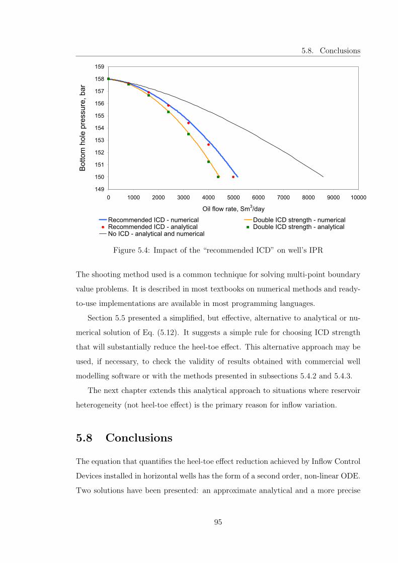
5.8. Conclusions
149
150
151
152
153
154
155
156
157
158
159
0 1000 2000 3000 4000 5000 6000 7000 8000 9000 10000
Oil flow rate, Sm3/day
Bot
tom
hol
e pr
essu
re, b
ar
Recommended ICD - numerical Double ICD strength - numericalRecommended ICD - analytical Double ICD strength - analyticalNo ICD - analytical and numerical
Figure 5.4: Impact of the “recommended ICD” on well’s IPR
The shooting method used is a common technique for solving multi-point boundary
value problems. It is described in most textbooks on numerical methods and ready-
to-use implementations are available in most programming languages.
Section 5.5 presented a simplified, but effective, alternative to analytical or nu-
merical solution of Eq. (5.12). It suggests a simple rule for choosing ICD strength
that will substantially reduce the heel-toe effect. This alternative approach may be
used, if necessary, to check the validity of results obtained with commercial well
modelling software or with the methods presented in subsections 5.4.2 and 5.4.3.
The next chapter extends this analytical approach to situations where reservoir
heterogeneity (not heel-toe effect) is the primary reason for inflow variation.
5.8 Conclusions
The equation that quantifies the heel-toe effect reduction achieved by Inflow Control
Devices installed in horizontal wells has the form of a second order, non-linear ODE.
Two solutions have been presented: an approximate analytical and a more precise
95

5.8. Conclusions
numerical one. These solutions allow one to estimate the:
• ICD design parameters that reduce the heel-toe effect to the required level.
• Impact of the ICD on the well’s inflow peformance relationship.
The practical utility of this approach been illustrated using published Troll oil field
data.
96
Chapter 6
Application of Inflow Control
Devices to Heterogeneous
Reservoirs
6.1 Introduction
This chapter proposes an analytical model for heterogeneous reservoirs that quan-
tifies the reduction of inflow variation along a horizontal well with ICDs installed.
This model allows one to estimate:
• The ICD design parameters that substantially reduce the inflow variation
caused by reservoir heterogeneity.
• The impact of a specific ICD completion on Inflow Performance Relationship
(IPR) of a long well completed in a heterogeneous reservoir.
6.2 Assumptions
The model presented in this chapter invokes the following assumptions with respect
to the inflow from the reservoir:
97
6.2. Assumptions
• Flow through the reservoir can be described by Darcy’s law.
• Steady or pseudo-steady state flow into the well.
• The distance between the well and the reservoir boundary is much longer than
the well length (or the boundary is parallel to the well).
• The perpendicular-to-the-well components of the reservoir pressure gradients
are much greater than the along-hole ones.
The chosen assumptions for the description of the wellbore flow are that:
• Friction and acceleration pressure losses between the toe and the heel are small
compared to the drawdown.
• The fluid is incompressible.
The above assumptions imply that the difference between the reservoir exter-
nal boundary pressure Pe and the tubing pressure P is constant throughout the
completion length:
Pe(l)− P (l) = ∆Pw = const (6.1)
The assumptions about the ICDs are as follows:
1. There is no flow in the annulus parallel to the base pipe, i.e. the fluid flows
from reservoir directly through ICD screens into the base pipe.
2. ICDs of the same “strength” are installed throughout the completion length.
3. The flow distribution along the wellbore’s internal flow conduit q(l) is “smooth”
(i.e. it has a continuous derivative).
These assumptions were previously discussed in section 5.2.
98
6.3. Problem Formulation
6.3 Problem Formulation
Let us analyse the impact of an ICD completion on the well inflow profile when the
well is completed in a heterogeneous reservoir.
The Specific Productivity Index, j, and hence the inflow, U , change stochastically
along the completion interval. A coefficient of variation will be used to quantify the
degree of these changes. Recall that the coefficient of variation of a random variable
is defined as the ratio of its standard deviation and its mean.
The annulus pressure Pa is equal to the base pipe pressure P for a conventional
completion (no ICD). Hence:
U(l) = j(l)∆Pw (6.2)
where ∆Pw is a constant independent of l. Eq. (6.2) shows that, in case of conven-
tional completion (no ICD), the coefficient of variation of specific inflow is equal to
that of the specific PI:
CoVU = CoV j (6.3)
ICD application reduces the variation of inflow so that:
CoVU < CoV j (6.4)
Inequality (6.4) may seem intuitively obvious to engineers familiar with the ICD
technology, however its rigorous mathematical proof requires considerable ingenuity.
The proof was suggested by Alexandr V. Usnich (Birchenko et al., 2009).
Let us consider the ratio of the two coefficients of variation, CoVU/CoV j.
This ratio equals unity for a conventional completion and decreases monotonically
with increasing ICD strength. The magnitude of this decrease is a quantitative
measure of the equalisation of the inflow along the completion length due to the
ICD. The objective of this work is to develop a mathematical model linking the
ratio of the two coefficients of variation with the well parameters (such as ICD
“strength”, drawdown, etc.)
99

6.4. Solution
6.4 Solution
The solution for inflow to an ICD well was presented in section 5.3. Eq. (5.10) is of
limited use for a “quick-look” analysis if the local specific productivity index varies
substantially along the completion interval since:
1. The exact shape of the productivity profile j(l) is often unknown:
• Detailed measurements (logging) are not always feasible.
• The productivity index changes with time (e.g. due to fluid saturation
changes).
2. In general one needs to evaluate the integral (5.10) numerically even if j(l) is
known (or can be estimated).
The engineering team that develops each well drilling proposal will normally
define an expected range of values for the specific productivity index, j, as part of
the proposal. These could be based on:
• Well log data.
• Reservoir models.
• Production performance of similar wells in the same field.
This range of values may take a number of forms. For instance, in its simplest form
it could comprise of only three values: pessimistic (P90), most probable (P50) and
optimistic (P10). Ideally, a complete specification of j would be available in the
form of a probability density function (p.d.f.). In the case when j depends on some
other parameters and information about their distribution is available this density
can be estimated, for example, via Monte-Carlo simulation.
It is often easier to make a judgement about the statistical distribution of the
specific productivity index, η(j), rather than its spatial distribution j(l). This allows
one to transform formula (5.10) into
qw = L
∫ j2
j1
−1 +√
1 + 4a∆Pwj2
2ajη(j) dj (6.5)
100
6.4. Solution
Calculation of the coefficient of variation requires mean and mean square values of
the specific inflow rate. The mean specific inflow rate is the ratio of the well flow
rate to its length:
〈U〉 = qw/L =
∫ j2
j1
−1 +√
1 + 4a∆Pwj2
2ajη(j) dj (6.6)
Similarly, its mean square value is calculated as follows:
〈U2〉 =
∫ j2
j1
(−1 +
√1 + 4a∆Pwj2
2aj
)2
η(j) dj (6.7)
The choice of the method for solving the integrals (6.6) and (6.7) depends on
the functional form of η(j), the p.d.f. of the specific PI. Notably, these integrals
can be solved analytically for a piecewise linear p.d.f. (e.g. a uniform or triangular
distribution). The corresponding solutions are presented below in subsections 6.4.1
and 6.4.2. When the density function has a more complex form (e.g. a normal or
log-normal distribution) the integrals have to be evaluated numerically.
6.4.1 Uniform Distribution of Specific Productivity Index
Generally speaking, a uniform distribution of the specific productivity index is un-
likely to be encountered in practice. In fact, petro-physical quantities are usually
modelled by a normal or log-normal distribution. However, the data required to
determine the distribution parameters with sufficient precision is often unavailable.
A uniform distribution may be a sensible starting assumption when data is scarce.
Assuming that j is uniformly distributed between two values j1 and j2, j1 ≤ j2,
its density function is as follows:
η(j) =
1/(j2 − j1) for j1 ≤ j ≤ j2
0 otherwise
(6.8)
101

6.4. Solution
In this case:
qw = 〈U〉L =IU(j2)− IU(j1)
j2 − j1L (6.9)
andCoVU
CoV j=
(j2 + j1)√
3 (〈U2〉 − 〈U〉2)〈U〉(j2 − j1)
(6.10)
where
〈U2〉 =SU(j2)− SU(j1)
j2 − j1(6.11)
with
IU(j) =
√1 + 4a∆Pwj2 − ln
(1 +
√1 + 4a∆Pwj2
)2a
(6.12)
SU(j) =1
2a2j
(−1 + 2a∆Pwj
2 +√
1 + 4a∆Pwj2−
−2j√a∆Pw arcsinh
(2j√a∆Pw
)) (6.13)
6.4.2 Triangular Distribution of Specific Productivity Index
The most probable, or modal value is often known within reasonable error margins
in addition to knowledge about the minimum and maximum values of the specific
PI. The specific productivity index j may then be modelled by the (more complex)
triangular distribution. This is a legitimate approach if a triangular distribution can
be fitted to the field data with accuracy similar to that of the more common normal
or log-normal distributions.
The p.d.f. of a triangular distribution is as follows:
η(j) =
2(j − j1)/(j2 − j1)/(jm − j1) for j1 ≤ j ≤ jm
2(j2 − j)/(j2 − j1)/(j2 − jm) for jm ≤ j ≤ j2
0 otherwise
(6.14)
102

6.5. Case Study
Then
qw = 〈U〉L =2L
j2 − j1
(IUj(jm)− IUj(j1)− j1 (IU(jm)− IU(j1))
jm − j1+
+j2 (IU(j2)− IU(jm))− IUj(j2) + IUj(jm)
j2 − jm
)(6.15)
and
CoVU
CoV j=j2 + jm + j1〈U〉
√2 (〈U2〉 − 〈U〉2)
j21 + j2
2 + j2m − j1j2 − j1jm − j2jm
(6.16)
where
〈U2〉 =2
j2 − j1
(SUj(jm)− SUj(j1)− j1 (SU(jm)− SU(j1))
jm − j1+
+j2 (SU(j2)− SU(jm))− SUj(j2) + SUj(jm)
j2 − jm
)(6.17)
with
IUj =1
2a
(−j +
j√
1 + 4aj2∆Pw2
+arcsinh
(2j√a∆Pw
)4√a∆Pw
)(6.18)
SUj(j) =∆Pj2/2− IU(j)
a(6.19)
and functions IU and SU defined by (6.12) and (6.13) respectively.
6.5 Case Study
This case study shows how the proposed model for a uniform distribution can be
used in practice for the following two cases:
1. Highly Productive Reservoir
2. Medium Productivity Reservoir.
This is done to quantitatively illustrate the dependence between the specific PI and
ICD “strength” required to reduce inflow variations.
103
6.5. Case Study
6.5.1 Highly Productive Reservoir
Let us consider a 1 km long well completed in a prolific heterogeneous reservoir
(Table 6.1). The anticipated PI of the well is 2 000 Sm3/day/bar. A drawdown,
∆Pr, of 0.5 bar is required for a conventional completion to achieve the target well
rate of 1 000 Sm3/day. Pressure drop introduced by conventional completion is
usually negligible compared to the drawdown:
∆Pw ≈ ∆Pr = 0.5 bar (6.20)
Well length L 1 000 m
Well PI J 2 000 Sm3/day/bar
Minimum value of specific PI j1 0.5 Sm3/day/bar/m
Maximum value of specific PI j2 3.5 Sm3/day/bar/m
Target well flow rate qw 1 000 Sm3/day
In-situ fluid density ρ 800 kg/m3
In-situ fluid viscosity µ 1.7 cp
Formation volume factor B 1.2 Rm3/Sm3
Length of the ICD joint lICD 12.2 m
Table 6.1: Highly productive reservoir case study data
The inflow distribution along the completion is expected to be highly uneven and
uncertain due to complex reservoir geology. The local specific productivity index
is anticipated to be within the range of 0.5 - 3.5 Sm3/day/bar/m. Subject to the
assumptions stated in section 6.2, the inflow to the conventional completion will be
proportional to the local specific productivity index. This implies a 7-fold variation
of specific inflow rate for the above case.
A completion combining ICDs and annular flow isolation will improve oil recovery
by smoothing out the specific inflow rate variations and increasing oil sweep efficiency
along the above horizontal well.
104

6.5. Case Study
The uniform distribution model (formula (6.9), subsection 6.4.1) predicts that
“1.6 bar” ICD completion with ∆Pw of 1 bar will produce 1 070 Sm3/day. That
is, the “1.6 bar” ICD completion reduced well productivity by approximately 50%
(for the target rate), but also delivered an improved degree of inflow equalisation
(Figure 6.1). The grey line in Figure 6.1 was obtained using formula (5.9). The
specific inflow rate variation is considerably smaller than for a conventional com-
pletion. Namely, the CoVU/CoV j ratio of 0.52 for the “1.6 bar” ICD case can be
interpreted as almost a 50% reduction of the difference between regions of high and
low specific inflow rate.
0
0.5
1
1.5
2
2.5
3
3.5
4
0 200 400 600 800 1000
Measured depth (from the heel), m
Spe
cific
PI,
Sm
3 /day
/ ba
r / m
0
0.5
1
1.5
2
2.5
3
3.5
4
Spe
cific
inflo
w ra
te, S
m3 /d
ay /
mSpecific PI Specific Inflow with '1.6 bar' ICDs and no annular flow
Figure 6.1: An example of inflow equalisation with ICDs
An increase in the ICD strength gives an even more uniform inflow at the cost
of further reduction of well inflow performance. This is illustrated in figures 6.2 and
6.3 which were derived using formulae (6.9) and (6.10) for ∆Pw = 1 bar.
6.5.2 Medium Productivity Reservoir
The specific productivity index is the key parameter in ICD completion design. The
majority of ICD installations to date are in reservoirs with an average permeability
105

6.5. Case Study
0
0.2
0.4
0.6
0.8
1
1.2
0 0.001 0.002 0.003 0.004 0.005 0.006 0.007
Channel ICD strength, bar/(Rm3/day)2
CoV
ratio
0
500
1000
1500
2000
2500
Wel
l flo
w ra
te, S
m3 /d
ay
CoV ratio Well flow rate
Figure 6.2: Dependence of inflow equalisation and well productivity on ICD strengthfor channel ICDs in a highly productive reservoir
of one Darcy or greater (Table 2.7). In order to illustrate the importance of this
parameter let us now consider the case with 10 times lower PI (200 Sm3/day/bar)
and 10 times higher total pressure drop (10 bar). Such modifications (Table 6.2)
would not change the inflow performance of conventional completion as it is the
product of the PI and the pressure drop that determines the inflow rate. However,
the performance of an ICD completion will be different since the inflow is no longer
proportional to the above mentioned product in this case.
Well’s PI J 200 Sm3/day/bar
Minimum value of specific PI j1 0.05 Sm3/day/bar/m
Maximum value of specific PI j2 0.35 Sm3/day/bar/m
Total pressure drop at the heel ∆Pw 10 bar
Table 6.2: Medium productivity reservoir case study
According to formulae (6.9) and (6.10), the flow rate of a “1.6 bar” ICD well is
1 720 Sm3/day and the (CoVU/CoV j) ratio is 0.85 for the medium productivity
reservoir. This implies that the well flow rate and specific inflow rate variation were
106
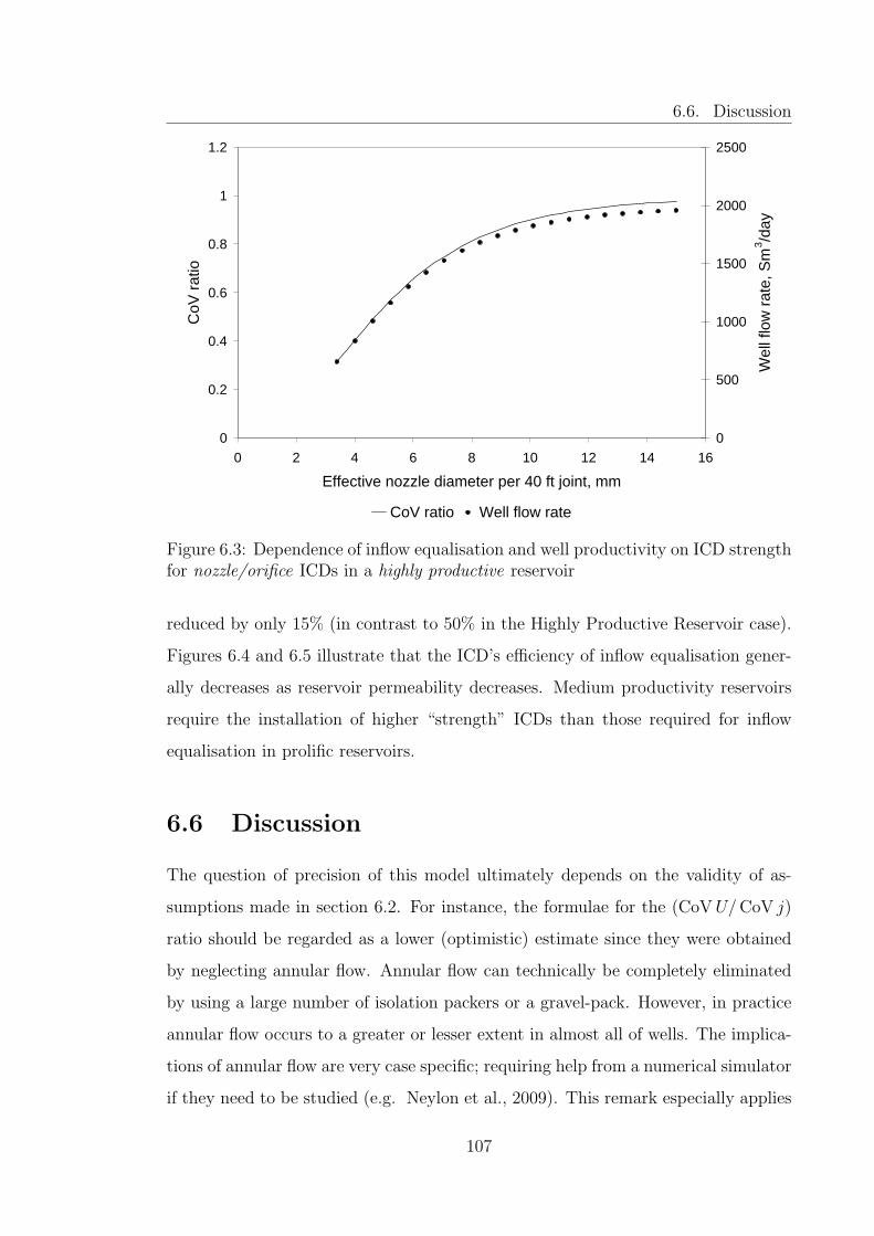
6.6. Discussion
0
0.2
0.4
0.6
0.8
1
1.2
0 2 4 6 8 10 12 14 16
Effective nozzle diameter per 40 ft joint, mm
CoV
ratio
0
500
1000
1500
2000
2500
Wel
l flo
w ra
te, S
m3 /d
ay
CoV ratio Well flow rate
Figure 6.3: Dependence of inflow equalisation and well productivity on ICD strengthfor nozzle/orifice ICDs in a highly productive reservoir
reduced by only 15% (in contrast to 50% in the Highly Productive Reservoir case).
Figures 6.4 and 6.5 illustrate that the ICD’s efficiency of inflow equalisation gener-
ally decreases as reservoir permeability decreases. Medium productivity reservoirs
require the installation of higher “strength” ICDs than those required for inflow
equalisation in prolific reservoirs.
6.6 Discussion
The question of precision of this model ultimately depends on the validity of as-
sumptions made in section 6.2. For instance, the formulae for the (CoVU/CoV j)
ratio should be regarded as a lower (optimistic) estimate since they were obtained
by neglecting annular flow. Annular flow can technically be completely eliminated
by using a large number of isolation packers or a gravel-pack. However, in practice
annular flow occurs to a greater or lesser extent in almost all of wells. The implica-
tions of annular flow are very case specific; requiring help from a numerical simulator
if they need to be studied (e.g. Neylon et al., 2009). This remark especially applies
107
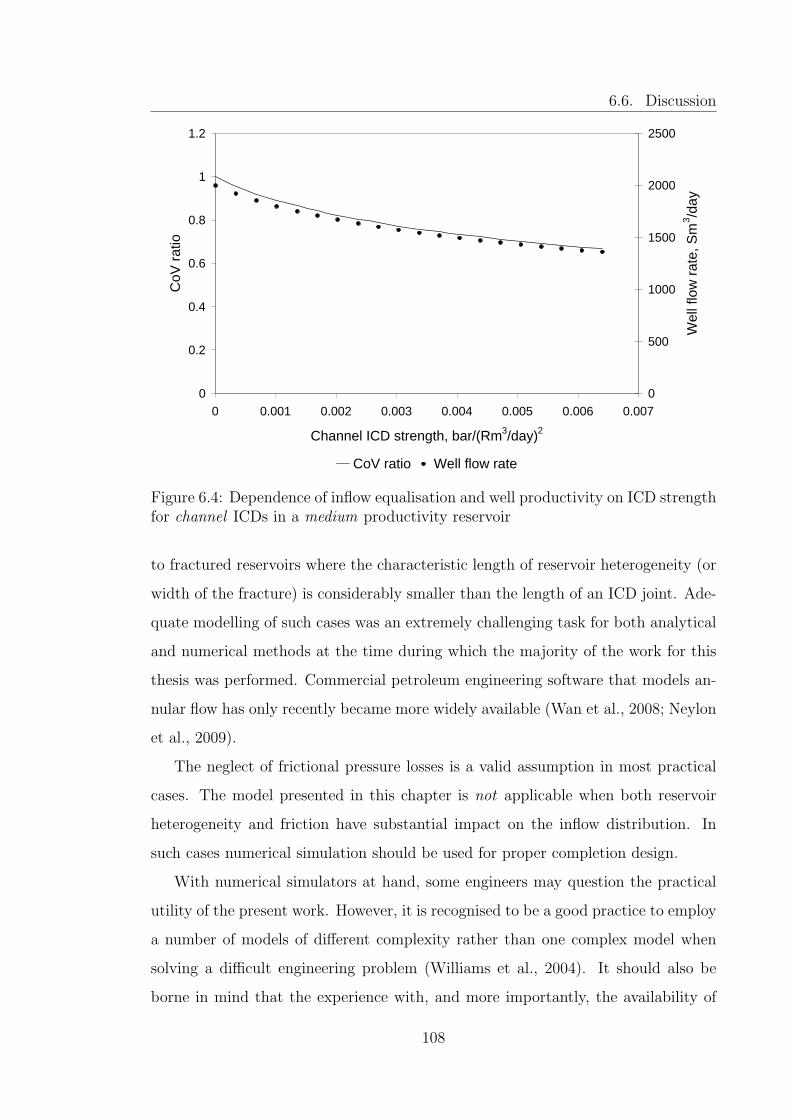
6.6. Discussion
0
0.2
0.4
0.6
0.8
1
1.2
0 0.001 0.002 0.003 0.004 0.005 0.006 0.007
Channel ICD strength, bar/(Rm3/day)2
CoV
ratio
0
500
1000
1500
2000
2500
Wel
l flo
w ra
te, S
m3 /d
ay
CoV ratio Well flow rate
Figure 6.4: Dependence of inflow equalisation and well productivity on ICD strengthfor channel ICDs in a medium productivity reservoir
to fractured reservoirs where the characteristic length of reservoir heterogeneity (or
width of the fracture) is considerably smaller than the length of an ICD joint. Ade-
quate modelling of such cases was an extremely challenging task for both analytical
and numerical methods at the time during which the majority of the work for this
thesis was performed. Commercial petroleum engineering software that models an-
nular flow has only recently became more widely available (Wan et al., 2008; Neylon
et al., 2009).
The neglect of frictional pressure losses is a valid assumption in most practical
cases. The model presented in this chapter is not applicable when both reservoir
heterogeneity and friction have substantial impact on the inflow distribution. In
such cases numerical simulation should be used for proper completion design.
With numerical simulators at hand, some engineers may question the practical
utility of the present work. However, it is recognised to be a good practice to employ
a number of models of different complexity rather than one complex model when
solving a difficult engineering problem (Williams et al., 2004). It should also be
borne in mind that the experience with, and more importantly, the availability of
108
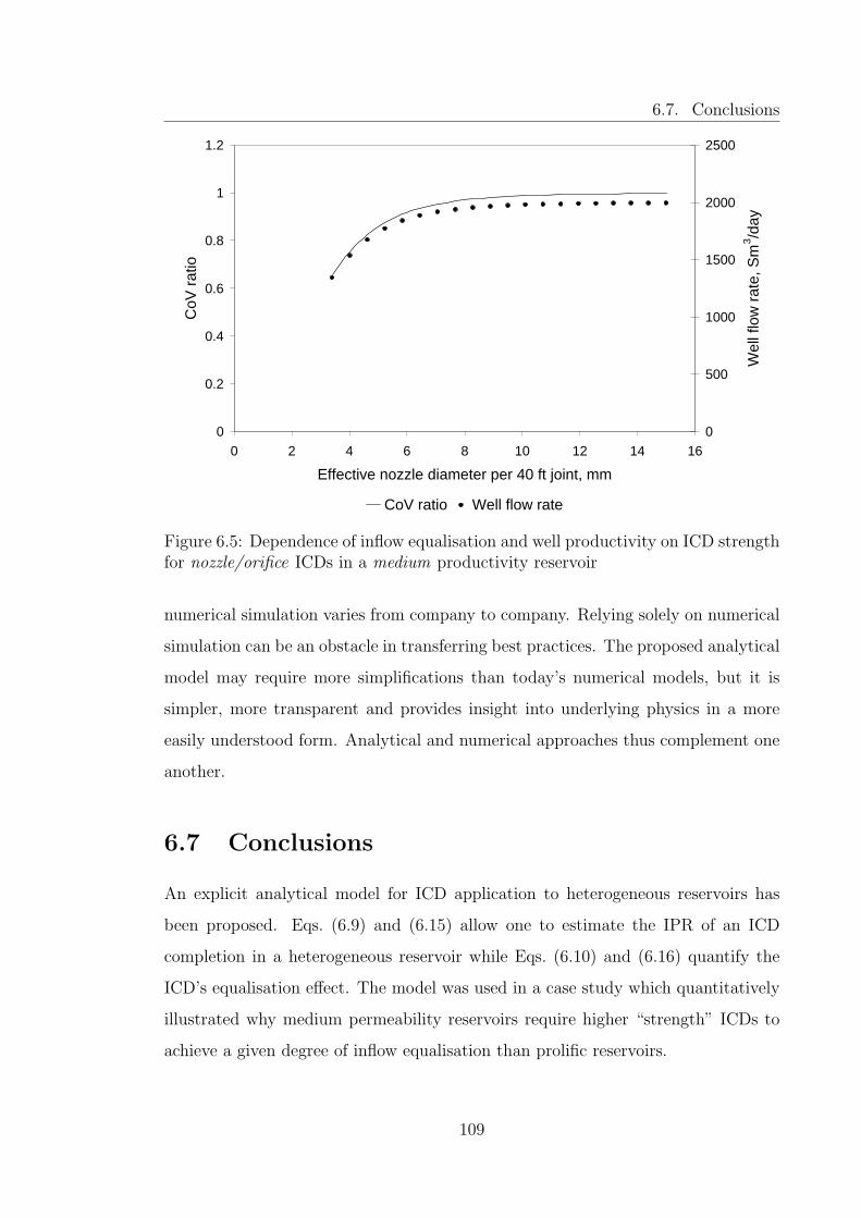
6.7. Conclusions
0
0.2
0.4
0.6
0.8
1
1.2
0 2 4 6 8 10 12 14 16
Effective nozzle diameter per 40 ft joint, mm
CoV
ratio
0
500
1000
1500
2000
2500
Wel
l flo
w ra
te, S
m3 /d
ay
CoV ratio Well flow rate
Figure 6.5: Dependence of inflow equalisation and well productivity on ICD strengthfor nozzle/orifice ICDs in a medium productivity reservoir
numerical simulation varies from company to company. Relying solely on numerical
simulation can be an obstacle in transferring best practices. The proposed analytical
model may require more simplifications than today’s numerical models, but it is
simpler, more transparent and provides insight into underlying physics in a more
easily understood form. Analytical and numerical approaches thus complement one
another.
6.7 Conclusions
An explicit analytical model for ICD application to heterogeneous reservoirs has
been proposed. Eqs. (6.9) and (6.15) allow one to estimate the IPR of an ICD
completion in a heterogeneous reservoir while Eqs. (6.10) and (6.16) quantify the
ICD’s equalisation effect. The model was used in a case study which quantitatively
illustrated why medium permeability reservoirs require higher “strength” ICDs to
achieve a given degree of inflow equalisation than prolific reservoirs.
109
Chapter 7
Conclusions and Future Work
7.1 Conclusions
The work presented in this thesis can be summarized as follows:
1. Major aspects dictating the choice between ICVs and ICDs have been re-
viewed. Figure 2.1 and Table 2.1 provide basis for the selection criteria. The
value difference between ICV and ICD has been quantified where appropri-
ate. As usual, full economic quantification of the value associated with each
completion remains a field specific task.
2. Well completion design has been shown to reduce the impact of geostatistical
uncertainty on the production forecast using the uncertainty quantification
methodology as applied in reservoir engineering. The study of the PUNQ-S3
reservoir found that a well completion designed based on:
• ICDs increased the mean recovery with a limited decrease in of risk.
• ICVs further increased mean recovery and reduced the risk compared to
the base case by 50%.
3. An explicit analytical model for turbulent flow in a highly deviated wellbore
has been developed and verified in Chapter 4. The model is consistent with the
110

7.1. Conclusions
semi-analytical models of Seines et al. (1993), Halvorsen (1994) and Penmatcha
et al. (1999) as well as with the results of numerical simulations performed in
commercial well modelling software.
4. The equation that quantifies the heel-toe effect reduction achieved by Inflow
Control Devices installed in horizontal wells has the form of a second order,
non-linear ODE. Two solutions have been presented: an approximate analyt-
ical and a more precise numerical one. These solutions allow one to estimate
the:
• ICD design parameters that reduce the heel-toe effect to the required
level.
• Impact of the ICD on the well’s inflow peformance relationship.
The practical utility of this approach been illustrated using published Troll oil
field data.
5. An explicit analytical model for ICD application to heterogeneous reservoirs
has been proposed in Chapter 6. Eqs. (6.9) and (6.15) allow one to estimate the
IPR of an ICD completion in a heterogeneous reservoir while Eqs. (6.10) and
(6.16) quantify the ICD’s equalisation effect. The model was used in a case
study which quantitatively illustrated why medium permeability reservoirs
require higher “strength” ICDs to achieve a given degree of inflow equalisation
than prolific reservoirs.
6. The trade-off between well productivity and inflow equalisation is a key engi-
neering issue when applying ICD technology. Solutions presented in Chapters
5 and 6 give general guidance for choosing an ICD design as well as provide
specific quantitative recommendations.
111

7.2. Future Work
7.2 Future Work
Some possible extensions for this work are:
Chapter 3. 1. Further investigate the dependence of results on the choice of the
Base Case (more aggressive production strategy, gas reinjection
etc.).
2. Investigate the impact of advanced well completion on other types
of reservoir uncertainty (e.g. relative permeability curves, fluid con-
tacts, aquifer etc.)
3. Employ a larger number of representative reservoir realisations,
which could involve adaptive selection of the geomodel parameters
to match the history data and assess their uncertainty (see, e.g.,
Demyanov et al., 2004).
4. Model the annular flow in ICD completion.
Chapter 5. Develop guidelines on acceptable magnitudes of the heel-toe effect.
Chapter 6. 1. Implement numerical solution of integrals (6.6) and (6.7) for arbi-
trary form of p.d.f. of specific productivity index.
2. Develop guidelines on acceptable values of inflow’s coefficient of
variation.
112

Bibliography
Abramowitz, M., Stegun, I., 1965. Handbook of Mathematical Functions with For-
mulas, Graphs, and Mathematical Table. Courier Dover Publications. 68
Akram, N., Hicking, S., Blythe, P., Kavanagh, P., Reijnen, P., Mathieson, D., 2001.
Intelligent well technology in mature assets. In: Offshore Europe.
URL http://dx.doi.org/10.2118/71822-MS 26
Al-Kasim, F. T., Tevik, S., Jakobsen, K. A., Tang, Y., Jalali, Y., 2002. Remotely
controlled in-situ gas lift on the norne subsea field. In: SPE Annual Technical
Conference and Exhibition.
URL http://dx.doi.org/10.2118/77660-MS 26
Al-Khelaiwi, F., 2007. Private communication. 45
Al-Khelaiwi, F., Davies, D., 2007. Inflow Control Devices: Application and value
quantification of a developing technology. In: SPE International Oil Conference
and Exhibition in Mexico.
URL http://dx.doi.org/10.2118/108700-MS 2
Al-Khelaiwi, F. T., Muradov, K. M., Davies, D. R., Olowoleru, D. K., 2009. Ad-
vanced well flow control technologies can improve well clean-up. In: 8th European
Formation Damage Conference.
URL http://dx.doi.org/10.2118/122267-MS 30
Augustine, J., Mathis, S., Nguyen, H., Gann, C., Gill, J., 2008. World’s first gravel-
packed inflow-control completion. SPE Drilling & Completion 23 (1), 61–67.
URL http://dx.doi.org/10.2118/103195-PA 13, 81
113
Bibliography
Augustine, J. R., 2002. An investigation of the economic benefit of Inflow Control
Devices on horizontal well completions using a reservoir-wellbore coupled model.
In: European Petroleum Conference.
URL http://dx.doi.org/10.2118/78293-MS 31
Babu, D. K., Odeh, A. S., November 1989. Productivity of a horizontal well. SPE
Reservoir Engineering 4 (4), 417–421.
URL http://dx.doi.org/10.2118/18298-PA 58
Baker, L., 1992. C Mathematical Function Handbook. McGraw-Hill, Inc. New York,
NY, USA. 68
Bellarby, J. E., Denholm, A., Grose, T., Norris, M., Stewart, A., 2003. Design
and implementation of a high rate acid stimulation through a subsea intelligent
completion. In: Offshore Europe.
URL http://dx.doi.org/10.2118/83950-MS 31
Birchenko, V., Bejan, A., Usnich, A., Davies, D., November 2009. Application of
Inflow Control Devices to heterogeneous reservoirs, preprint PETROL2802 sub-
mitted to Journal of Petroleum Science and Engineering. 99
Brouwer, D., Jansen, J.-D., 2004. Dynamic optimization of waterflooding with smart
wells using optimal control theory. SPE Journal 9 (4), 391–402.
URL http://dx.doi.org/10.2118/78278-PA 5
Carter, J., 2006. PUNQ-S3 Truth Case. Imperial College London.
URL http://www3.imperial.ac.uk/earthscienceandengineering/
research/perm/punq-s3model/truthcase/ 41
Clemo, T., 2006. Flow in perforated pipes: A comparison of models and experiments.
SPE Production & Operations 21 (2), 302–311.
URL http://dx.doi.org/10.2118/89036-PA 125
Coquereaux, R., Grossmann, A., Lautrup, B. E., 1990. Iterative method for calcu-
lation of the weierstrass elliptic function. IMA J Numer Anal 10 (1), 119–128.
68
114

Bibliography
de Best, L., van den Berg, F., 2006. Smart fieldsmaking the most of our assets. In:
SPE Russian Oil and Gas Technical Conference and Exhibition.
URL http://dx.doi.org/10.2118/103575-MS xii, 28, 29
de Montleau, P., Cominelli, A., Neylon, K., Rowan, D., Pallister, I., Tesaker, O., Ny-
gard, I., September 2006. Production optimization under constraints using adjoint
gradients. In: 10th European Conference on the Mathematics of Oil Recovery. 11
Demyanov, V., Sabbey, S., Christie, M., 2004. Neighbourhood algorithm with geo-
statistical simulations for uncertainty quantification reservoir modelling: PUNQ-
S3 case study. In: 9th European Conference on Mathematics in Oil Recovery.
112
Dikken, B. J., November 1990. Pressure drop in horizontal wells and its effect on
production performance. Journal of Petroleum Technology 42 (11), 1426–1433.
URL http://dx.doi.org/10.2118/19824-PA 6, 52
Drakeley, B. K., Douglas, N. I., Haugen, K. E., Willmann, E., 2001. Application of
reliability analysis techniques to intelligent wells. In: Offshore Technology Con-
ference.
URL http://dx.doi.org/10.4043/13028-MS 28
Eckhardt, U., 1980. Algorithm 549: Weierstrass’ elliptic functions. ACM Trans.
Math. Softw. 6 (1), 112–120. 68
Floris, F., Bush, M., Cuypers, M., Roggero, F., Syversveen, A.-R., May 2001. Meth-
ods for quantifying the uncertainty of production forecasts: a comparative study.
Petroleum Geoscience 7, 87–96. 10, 41
Freyer, R., Huse, A., 2002. Swelling packer for zonal isolation in open hole screen
completions. In: European Petroleum Conference.
URL http://dx.doi.org/10.2118/78312-MS 13
Gai, H., 2002. A method to assess the value of intelligent wells. In: SPE Asia Pacific
Oil and Gas Conference and Exhibition.
URL http://dx.doi.org/10.2118/77941-MS 39
115

Bibliography
Gao, C., Rajeswaran, T., Nakagawa, E., 2007. A literature review on smart well
technology. In: SPE Production and Operations Symposium.
URL http://dx.doi.org/10.2118/106011-MS 2, 8, 21
Goode, P., Kuchuk, F., August 1991. Inflow performance of horizontal wells. SPE
Reservoir Engineering 6 (3), 319–323.
URL http://dx.doi.org/10.2118/21460-PA 58
Goode, P., Wilkinson, D., August 1991. Inflow performance of partially open hori-
zontal wells. Journal of Petroleum Technology 43 (8), 983–987.
URL http://dx.doi.org/10.2118/19341-PA 58
Haaland, A., Rundgren, G., Johannessen, ., 2005. Completion technology on troll-
innovation and simplicity. In: Offshore Technology Conference.
URL http://dx.doi.org/10.4043/17113-MS 4
Haaland, S., 1983. Simple and explicit formulas for the friction factor in turbulent
pipe flow. Journal of Fluids Engineering 105 (1), 89–90. 52, 127
Halliburton, 2009. NetoolTM near wellbore and completion hydraulics simulation
software. 16, 88
Halvorsen, G., July 1994. Discussion of considering wellbore friction effects in plan-
ning horizontal wells. Journal of Petroleum Technology 46 (6), 620. 53, 73, 76,
111, 133
Han, J. T., 2003. There is value in operational flexibility: An intelligent well appli-
cation. In: SPE Hydrocarbon Economics and Evaluation Symposium.
URL http://dx.doi.org/10.2118/82018-MS 38
Haug, B., 1992. The second long-term horizontal well test in troll: Successful pro-
duction from a 13-in. oil column with the well partly completed in the water zone.
In: SPE Annual Technical Conference and Exhibition.
URL http://dx.doi.org/10.2118/24943-MS 17
116
Bibliography
Haugen, V., Fagerbakke, A.-K., Samsonsen, B., Krogh, P., 2006. Subsea smart
multilateral wells increase reserves at Gullfaks South Statfjord. In: SPE/DOE
Symposium on Improved Oil Recovery.
URL http://dx.doi.org/10.2118/95721-MS 25
Helmy, M., Veselka, A., Benish, T., Yeh, C., Asmann, M., Yeager, D., Martin, B.,
Barry, M., 2006. Application of new technology in the completion of ERD wells,
Sakhalin-1 development. In: SPE Russian Oil and Gas Technical Conference and
Exhibition.
URL http://dx.doi.org/10.2118/103587-MS 82
Hembling, D., Sunbul, A., Salerno, G., 2007. Advanced well completions result in
enhanced well productivity and recovery in Saudi Aramco’s offshore fields. In:
Asia Pacific Oil and Gas Conference and Exhibition.
URL http://dx.doi.org/10.2118/108877-MS 13
Henriksen, K., Gule, E., Augustine, J., 2006. Case Study: The Application of Inflow
Control Devices in the Troll Oil Field. In: SPE Europec/EAGE Annual Confer-
ence and Exhibition.
URL http://dx.doi.org/10.2118/100308-MS 32, 82, 83, 90, 91
Hill, A., Zhu, D., May 2008. The Relative Importance of Wellbore Pressure Drop
and Formation Damage in Horizontal Wells. SPE Production & Operations 23 (2),
232–240.
URL http://dx.doi.org/10.2118/100207-PA 54, 132
Jain, A., 1976. Accurate explicit equation for friction factor. Journal of the Hy-
draulics Division 102 (5), 674–677. 53
Johansen, T. E., Khoriakov, V., 2007. Iterative techniques in modeling of multi-
phase flow in advanced wells and the near well region. Journal of Petroleum Science
and Engineering 58 (1-2), 49 – 67.
URL http://dx.doi.org/10.1016/j.petrol.2006.11.013 6, 74, 79, 88, 91
Joshi, S. D., 1991. Horizontal Well Technology. PennWell Books. 52, 54
117

Bibliography
Katamish, H., Steel, N., Smith, A., Thompson, P., 2005. WDDM: The jewel of the
Nile. In: SPE Europec/EAGE Annual Conference.
URL http://dx.doi.org/10.2118/94123-MS 32
Kavle, V., Elmsallati, S., Mackay, E., Davies, D., 2006. Impact of intelligent wells
on oilfield scale management. In: SPE Europec/EAGE Annual Conference and
Exhibition.
URL http://dx.doi.org/10.2118/100112-MS 31
Konopczynski, M., 2008. Private communication. 12
Kulkarni, R., Belsvik, Y., Reme, A., 2007. Smart-well monitoring and control:
Snorre B experience. In: SPE Annual Technical Conference and Exhibition.
URL http://dx.doi.org/10.2118/109629-MS 28
Landman, M. J., 1994. Analytic modelling of selectively perforated horizontal wells.
Journal of Petroleum Science and Engineering 10 (3), 179 – 188.
URL http://dx.doi.org/10.1016/0920-4105(94)90079-5 53
Lau, H. C., Deutman, R., Al-Sikaiti, S., Adimora, V., 2001. Intelligent internal gas
injection wells revitalise mature S.W. Ampa field. In: SPE Asia Pacific Improved
Oil Recovery Conference.
URL http://dx.doi.org/10.2118/72108-MS 26
Leslie, K. J., Michaels, M. P., No. 3, 1997. The real power of Real Options. The
McKinsey Quarterly. 39
Manceau, E., Mezghani, M., Zabalza-Mezghani, I., Roggero, F., 2001. Combination
of experimental design and joint modeling methods for quantifying the risk asso-
ciated with deterministic and stochastic uncertainties - an integrated test study.
In: SPE Annual Technical Conference and Exhibition.
URL http://dx.doi.org/10.2118/71620-MS 35
Maplesoft, 2009. MapleTM mathematical software. 68
118

Bibliography
Mathieson, D., Rogers, J., Rajagopalan, S., McManus, R., 2003. Reliability assur-
ance, managing the growth of intelligent completion technology. In: SPE Annual
Technical Conference and Exhibition.
URL http://dx.doi.org/10.2118/84327-MS 28
McIntyre, A., Adam, R., Augustine, J., Laidlaw, D., 2006. Increasing oil recovery
by preventing early water and gas breakthrough in a West Brae horizontal well:
A case history. In: SPE/DOE Symposium on Improved Oil Recovery.
URL http://dx.doi.org/10.2118/99718-MS 82
Meum, P., Tndel, P., Godhavn, J.-M., Aamo, O. M., 2008. Optimization of smart
well production through nonlinear model predictive control. In: Intelligent Energy
Conference and Exhibition.
URL http://dx.doi.org/10.2118/112100-MS 12
Mjaavatten, A., Aasheim, R., Saelid, S., Gronning, O., 2008. A model for gas coning
and rate-dependent gas/oil ratio in an oil-rim reservoir. SPE Reservoir Evaluation
& Engineering 11 (5), 842–847.
URL http://dx.doi.org/10.2118/102390-PA 4, 79
Moen, T., Asheim, H., 2008. Inflow Control Device and near-wellbore interaction.
In: SPE International Symposium and Exhibition on Formation Damage Control.
URL http://dx.doi.org/10.2118/112471-MS 30
Moody, L., 1944. Friction factors for pipe flow. Trans. ASME 66 (8), 671–677. 18
Neylon, K., Reiso, E., Holmes, J., Nesse, O., 2009. Modeling well inflow control with
flow in both annulus and tubing. In: SPE Reservoir Simulation Symposium.
URL http://dx.doi.org/10.2118/118909-MS 6, 79, 107, 108
Nielsen, V. B. J., Piedras, J., Stimatz, G. P., Webb, T. R., 2002. Aconcagua, Camden
Hills, and King’s Peak fields, Gulf of Mexico, employ intelligent completion tech-
nology in unique field-development scenario. SPE Production & Facilities 17 (4),
236–240.
URL http://dx.doi.org/10.2118/80292-PA 4, 26
119

Bibliography
Novy, R., 1995. Pressure drops in horizontal wells: When can they be ignored. SPE
Reservoir Engineering Journal 10 (1), pp. 29–35.
URL http://dx.doi.org/10.2118/24941-PA 53
Ogoke, V., Aihevba, C., Marketz, F., 2006. Cost-effective life-cycle profile control
completion system for horizontal and multilateral wells. In: SPE Annual Technical
Conference and Exhibition.
URL http://dx.doi.org/10.2118/102077-MS 13
Olowoleru, D., Muradov, K., Al-Khelaiwi, F., Davies, D., 2009. Efficient intelligent
well cleanup using downhole monitoring. In: 8th European Formation Damage
Conference.
URL http://dx.doi.org/10.2118/122231-MS 30
Ouyang, L.-B., 2007. Uncertainty assessment on well performance prediction for
an oil well equipped with selected completions. In: Production and Operations
Symposium.
URL http://dx.doi.org/10.2118/106966-MS 38
Ouyang, L.-B., Aziz, K., 2000. A homogeneous model for gas-liquid flow in horizontal
wells. Journal of Petroleum Science and Engineering 27 (3-4), 119 – 128.
URL http://dx.doi.org/10.1016/S0920-4105(00)00053-X 125
Ouyang, L.-B., Huang, B., 2005. An evaluation of well completion impacts on the
performance of horizontal and multilateral wells. In: SPE Annual Technical Con-
ference and Exhibition.
URL http://dx.doi.org/10.2118/96530-MS 6, 79
Ozkan, E., Haciislamoglu, C. S. M., Raghavan, R., 1995. Effect of conductivity on
horizontal well pressure behavior. SPE Advanced Technology Series 3 (1), 85–94.
URL http://dx.doi.org/10.2118/24683-PA 53
Penmatcha, V., Arbabi, S., Aziz, K., 1999. Effects of pressure drop in horizontal
wells and optimum well length. SPE Journal 4 (3), 215–223.
URL http://dx.doi.org/10.2118/57193-PA x, 54, 73, 74, 76, 111
120

Bibliography
Qudaihy, D. A., Qahtani, H. A., Sunbul, A., Hembling, D., Salerno, G., 2006. The
evolution of advanced well completions results in enhanced well productivity and
recovery in Saudi Aramco’s offshore fields. In: IADC/SPE Asia Pacific Drilling
Technology Conference and Exhibition.
URL http://dx.doi.org/10.2118/103621-MS 26
Raffn, A., Hundsnes, S., Kvernstuen, S., Moen, T., 2007. ICD screen technology used
to optimize waterflooding in injector well. In: SPE Production and Operations
Symposium.
URL http://dx.doi.org/10.2118/106018-MS 5
Saggaf, M., March 2008. A vision for future upstream technologies. Journal of
Petroleum Technology 60 (3), 54–55, 94–98. 12
Salamy, S., Al-Mubarak, H., Hembling, D., Al-Ghamdi, M., 2006. Deployed smart
technologies enablers for improving well performance in tight reservoirscase: Shay-
bah field, Saudi Arabia. In: Intelligent Energy Conference and Exhibition.
URL http://dx.doi.org/10.2118/99281-MS 21
Salamy, S. P., 2005. Maximum reservoir contact (MRC) wells: A new generation of
wells for developing tight reservoir facies. In: SPE Distinguish Lecturer Series.
URL http://dx.doi.org/10.2118/108806-DL 1
Schlumberger, October 2002. TRFC-HN AP and TRFC-HN LP hydraulic flow con-
trol valves datasheet.
URL http://www.slb.com/media/services/completion/intelligent/trfc_
hn_ap.pdf 22
Schlumberger, 2009. Eclipse user manual. 83
Schulze-Riegert, R., Axmann, J., Haase, O., Rian, D., You, Y.-L., 2001. Optimiza-
tion methods for history matching of complex reservoirs. In: SPE Reservoir Sim-
ulation Symposium.
URL http://dx.doi.org/10.2118/66393-MS 35
121

Bibliography
Seines, K., Aavatsmark, I., Lien, S., Rushworth, P., October 1993. Considering
wellbore friction in planning horizontal wells. Journal of Petroleum Technology
45 (10), 994–1000.
URL http://dx.doi.org/10.2118/21124-PA xviii, 52, 53, 54, 71, 72, 76, 111,
133
Shahri, A. M., Kilany, K., Hembling, D., Lauritzen, J. E., Gottumukkala, V., Ogun-
yemi, O., Moreno, O. B., 2009. Best cleanup practices for an offshore sandstone
reservoir with ICD completions in horizontal wells. In: SPE Middle East Oil and
Gas Show and Conference.
URL http://dx.doi.org/10.2118/120651-MS 30
Sharma, A., Chorn, L., Han, J., Rajagopalan, S., 2002. Quantifying value creation
from intelligent completion technology implementation. In: European Petroleum
Conference.
URL http://dx.doi.org/10.2118/78277-MS 38
Silva, M., Portella, R., Izetti, R., Campos, S., 2005. Technologies trials of intelligent-
field implementation in Carmopolis field. In: SPE Annual Technical Conference
and Exhibition.
URL http://dx.doi.org/10.2118/95517-MS xii, 28, 31
Stair, C., Bruesewitz, E., Shivers, J., Rajasingam, D., Dawson, M., 2004. Na kika
completions overview: Challenges and accomplishments. In: Offshore Technology
Conference.
URL http://dx.doi.org/10.4043/16228-MS 29
Su, Z., Gudmundsson, J. S., 1998. Perforation inflow reduces frictional pressure loss
in horizontal wellbores. Journal of Petroleum Science and Engineering 19 (3-4),
223 – 232.
URL http://dx.doi.org/10.1016/S0920-4105(97)00047-8 125
Sunbul, A., Hembling, D., Qudaihy, D. A., Harbi, N. A., Salerno, G., 2007. The
evolution of advanced well completions to enhance well productivity and recovery
122

Bibliography
in Saudi Aramco’s offshore fields. In: SPE Middle East Oil and Gas Show and
Conference.
URL http://dx.doi.org/10.2118/105036-MS 26
Sunbul, A., Lauritzen, J., Hembling, D., Majdpour, A., Raffn, A., Zeybek, M.,
Moen, T., 2008. Case histories of improved horizontal well cleanup and sweep
efficiency with nozzle based Inflow Control Devices (ICD) in sandstone and car-
bonate reservoirs. In: SPE Saudi Arabia Section Technical Symposium. Paper
SPE 120795. 30
Usnich, A., 2008. Private communication. 63
van den Berg, F. G., 2007. Smart fieldsoptimizing existing fields. In: Digital Energy
Conference and Exhibition.
URL http://dx.doi.org/10.2118/108206-MS 12
Wan, J., Dale, B. A., Ellison, T. K., Benish, T. G., Grubert, M. A., 2008. Coupled
well and reservoir simulation models to optimize completion design and operations
for subsurface control. In: Europec/EAGE Conference and Exhibition.
URL http://dx.doi.org/10.2118/113635-MS 6, 45, 79, 108
Weatherford, 2008. WellfloTM petroleum engineering software.
URL http://www.ep-solutions.com/PDF/Literature/5943_WellFlo_
Software.pdf 73, 74
Wehunt, C., September 2006. Well performance with operating limits under reservoir
and completion uncertainties. SPE Drilling & Completion 21 (3), 200–211.
URL http://dx.doi.org/10.2118/84501-PA 38
Williams, G., Mansfield, M., MacDonald, D., Bush, M., 2004. Top-down reservoir
modelling. In: SPE Annual Technical Conference and Exhibition.
URL http://dx.doi.org/10.2118/89974-MS 35, 108
Wolfram, 2009. MathematicaTM mathematical software. 68
123

Bibliography
Zandvliet, M., Bosgra, O., Jansen, J., den Hof, P. V., Kraaijevanger, J., 2007. Bang-
bang control and singular arcs in reservoir flooding. Journal of Petroleum Science
and Engineering 58 (1-2), 186 – 200.
URL http://dx.doi.org/10.1016/j.petrol.2006.12.008 22
124

Appendix A
Friction Factor Calculation
Laboratory experiments suggest that inflow or outflow through perforations does
not change the friction factor radically (see, e.g., Su and Gudmundsson, 1998;
Ouyang and Aziz, 2000). However the debate over the pressure drop correlation
for perforated pipes remains open (Clemo, 2006). Current versions of commer-
cial petroleum software use the same correlations for perforated and blank (non-
perforated) pipes. We used a non-perforated pipe correlation since the broad ques-
tion of pressure drop correlation choice is beyond the scope of this work.
The model presented in the section 4.5 can be used with any correlation as long as
the assumption of constant friction factor remains valid. The average friction factor
and the error associated with the averaging can be also estimated with various
techniques. The approach outlined below is an example of how such estimations
can be done in principle. It is not an intrinsic part of the model and can be easily
changed if appropriate for a specific case.
The flow regime is determined by the Reynolds number. The Reynolds number
at the heel of a rate constrained well is:
Rehq =CrρBqwµD
(A.1)
Precise calculation of Reynolds number for a pressure constrained well is, generally
speaking, an iterative process because the flow rate at the heel is unknown. A first
125

Appendix A. Friction Factor Calculation
approximation of the Reynolds number can be readily obtained by neglecting the
frictional pressure losses:
Rehp0 =CrρBJsL∆Pw
µD(A.2)
Formula (4.55) can then be used to calculate the first approximation of flow rate.
Repetition of this process gives further, more precise, estimates. Black arrows in
Figure A.1 show the data that should be used repeatedly in such iterative process.
This procedure was found to converge extremely rapidly. The precision obtained
by the first approximation is usually sufficient for a “quick-look” deterministic anal-
ysis since the error it introduces is typically much smaller than that due to the
uncertainties associated with the:
• Friction factor correlation.
• Input parameters.
• Validity of the assumptions.
Two iterations may be required if this model is to be used in a more sophisticated
type of analysis (e.g. for uncertainty quantification or optimisation).
ModelPw
qnof
1st iteration
qi
Rei
i++1st iteration
Figure A.1: Reynolds number calculation for a pressure constrained well
126

Appendix A. Friction Factor Calculation
The above enables calculation of the Reynolds number at the heel of the well,
Reh. We will now discuss how this number is used to calculate the average friction
factor.
Flow at the toe of the well is laminar and the required friction factor for circular
pipes is:
f = 16/Re, Re < Rec (A.3)
Using Eq. (4.6) we define the average friction factor for the toe part of the completion
where laminar flow is present:
fl ≡⟨dPdx
⟩2ρ 〈v2〉
D (A.4)
One can show that it is equal to:
fl = 24/Rec ≈ 0.01 (A.5)
and the normalised mean-square error of the pressure gradient associated with this
averaging process is 2/√
5.
The critical Reynolds number Rec (the number at which the transition between
laminar and turbulent flow starts to take place) depends on flow configuration and,
strictly speaking, must be determined experimentally. The transition normally oc-
curs over a range of Reynolds numbers between 2300 and 3600. In this work we
will assume that Rec has a value of 2300 and that the transition to fully developed
turbulent flow happens rapidly at Rec (Figure 4.1).
The Fanning friction factor for fully developed turbulent flow in rough pipes can
be calculated using following formula (Haaland, 1983):
f =[3.6 log10
(6.9/Re+ (e/D)10/9
)]−2
(A.6)
Figure A.2 illustrates the averaging procedure we used to estimate the overall friction
factor:
1. The average friction factor for the section of the wellbore with laminar flow
(black dotted line) is estimated using formula (A.5).
127
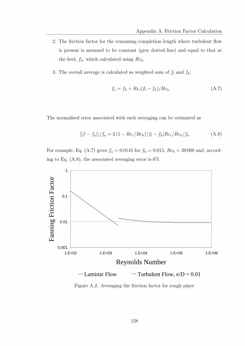
Appendix A. Friction Factor Calculation
2. The friction factor for the remaining completion length where turbulent flow
is present is assumed to be constant (grey dotted line) and equal to that at
the heel, fh, which calculated using Reh.
3. The overall average is calculated as weighted sum of fl and fh:
fa = fh +Rec(fl − fh)/Reh (A.7)
The normalised error associated with such averaging can be estimated as
〈|f − fa|〉/fa = 2 (1−Rec/Reh) |fl − fh|Rec/Reh/fa (A.8)
For example, Eq. (A.7) gives fa = 0.0145 for fh = 0.015, Reh = 20 000 and, accord-
ing to Eq. (A.8), the associated averaging error is 6%.
0.001
0.01
0.1
1
1.E+02 1.E+03 1.E+04 1.E+05 1.E+06
Reynolds Number
Fann
ing
Fric
tion
Fact
or
Laminar Flow Turbulent Flow, e/D = 0.01
Figure A.2: Averaging the friction factor for rough pipes
128

Appendix B
Pressure Drop due to Acceleration
Fluid that enters wellbore with a velocity directed nearly perpendicular to well-
bore has to be accelerated to acquire a velocity directed towards the heel. This
causes some pressure loss. Let us estimate the resulting pressure loss and compare
it to the frictional in order to determine whether the acceleration component of the
pressure drop can be neglected. Other assumptions (subsection 4.3.1) remain valid.
Also bear in mind that all formulae in this appendix are in SI units, however the
final inequality (4.3) is also valid in metric and field units.
The pressure gradient due to acceleration according to energy conservation law
is:dPadl
= − ddl
(ρv2
2
)(B.1)
The distribution of flow along the completion v(l) has to be known in order to
evaluate acceleration pressure drop. The fluid velocity at the toe of the well can be
assumed to be zero and flow rate at the heel is vh. Neither acceleration nor friction
normally have a significant effect on the flow rate along the completion’s length.
In fact, these effects are often neglected in conventional wells producing with flow
regimes other than mist flow. Hence, for an order-of-magnitude estimate, one can
reasonably assume that flow rate increases linearly with l from zero at the toe to vh
at the heel:
v(l) ≈ vhl/L (B.2)
129
Appendix B. Pressure Drop due to Acceleration
Substitution of formula (B.2) into (B.1) gives
dPadl≈ −ρvvh
L(B.3)
Dividing the Darcy-Weisbach equation (4.6) by (B.3) gives the ratio of the frictional
to the acceleration pressure losses:
dPfdPa≈ 2fLv
vhD(B.4)
The average value of fluid velocity, 〈v〉, is vh/2 leading to the average ratio of pressure
drops due to friction and acceleration becoming:
⟨dPfdPa
⟩≈ faL/D (B.5)
The acceleration pressure loss can thus be neglected when faL/D � 1.
130
Appendix C
The Upper Estimate of Frictional
Pressure Drop
Integration of Eq. (4.7) gives frictional pressure loss between the toe and the
heel:
Pt − Pw =CfρfB
2
D5
∫ L
0
q2(l) dl (C.1)
The upper estimate of the frictional pressure loss can thus be obtained from the
upper estimate of integral∫ L
0q2(l) dl. Let us examine the function q(l) describing
the flow rate distribution in the completion. It has the following properties:
1. q(0) = 0 (no flow at the toe);
2. q(L) = qw (the flow rate at the heel is known);
3. for any l1, l2 ∈ [0, L] q′(l2) > q′(l1) if l2 > l1 (the function is concave up).
Hence (Figure C.1):
q2(l) ≤ (qwl/L)2 for any l ∈ [0, L] (C.2)
Integration of the inequality (C.2) gives:
∫ L
0
q2(l) dl ≤ q2wL/3 (C.3)
131
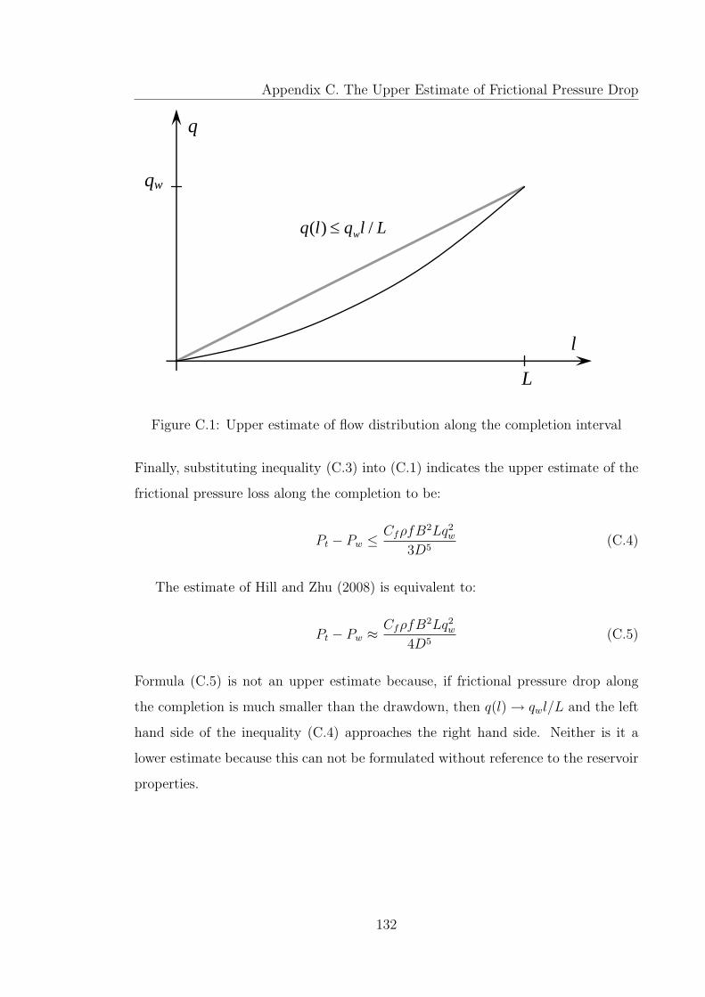
Appendix C. The Upper Estimate of Frictional Pressure Drop
qw
L
l
q
Llqlq w /)( ≤
Figure C.1: Upper estimate of flow distribution along the completion interval
Finally, substituting inequality (C.3) into (C.1) indicates the upper estimate of the
frictional pressure loss along the completion to be:
Pt − Pw ≤CfρfB
2Lq2w
3D5(C.4)
The estimate of Hill and Zhu (2008) is equivalent to:
Pt − Pw ≈CfρfB
2Lq2w
4D5(C.5)
Formula (C.5) is not an upper estimate because, if frictional pressure drop along
the completion is much smaller than the drawdown, then q(l)→ qwl/L and the left
hand side of the inequality (C.4) approaches the right hand side. Neither is it a
lower estimate because this can not be formulated without reference to the reservoir
properties.
132
Appendix D
Comparison to Halvorsen’s
Solution
According to Eqs. (A-23) and (A-24) of Seines et al. (1993):
qinf = Jsl∗∆Pw/2 (D.1)
Substitution of formula (4.66) into (4.60) gives
h∗p = 12 (D.2)
while substitution of formula (D.2) into (4.63) gives:
q∗w = 0.4805 Jsl∗∆Pw (D.3)
q∗w/qinf = 0.961 (D.4)
The precision can be further improved by using look-up tables or other more sophis-
ticated interpolation techniques instead of formula (4.61). For instance, using the
look-up table provided as supplementary data for this work, one can obtain even
more significant digits than provided by Halvorsen (1994): C∗p = 0.11472694553885
and then
133

Appendix D. Comparison to Halvorsen’s Solution
q∗w/qinf = 0.96019420783774.
Formula (4.56) gives the drawdown ratio of 0.34 for such a well (subsection 4.6.2).
134