analytical method for smooth interpolation of two-dimensional … · departamento de engenharia...

DEPARTAMENTO DE

ENGENHARIA MECÂNICA

AAnnaallyyttiiccaall MMeetthhoodd ffoorr SSmmooootthh IInntteerrppoollaattiioonn ooff

TTwwoo--DDiimmeennssiioonnaall SSccaallaarr FFiieellddss

Submitted in Partial Fulfilment of the Requirements for the Degree of Master in

Mechanical Engineering in the speciality of Energy and Environment

Author

Luís João Soares de Sousa Rodrigues

Advisors

António Gameiro Lopes, PhD

Igor Plaksin, PhD

Jury

Professor Doutor José Joaquim da Costa President

Professor da Universidade de Coimbra

Professor Doutor António Gameiro Lopes

Professor da Universidade de Coimbra

Professora Doutora Marta Cristina Cardoso de Oliveira Vowels

Professora da Universidade de Coimbra

Professor Doutor António Gameiro Lopes Advisors

Doutor Igor Plaksin

Coimbra, September 2015

Acknowledgements

Luís João Soares de Sousa Rodrigues iii

ACKNOWLEDGEMENTS

A very special acknowledgment is due to Dr. Igor Plaksin, whose continuous

support, over many years, made this endeavour possible.

Analytical Method for Smooth Interpolation of Two-Dimensional Scalar Fields

iv September 2015

Abstract

Luís João Soares de Sousa Rodrigues v

Abstract

The aim of the present MSc thesis is the accomplishment and evaluation of a

novel two-dimensional smooth interpolation method – in the form z= f(x,y) – from an

irregularly distributed dataset, that intrinsically assures gradient continuity and absence of

residuals at the input data points, whilst offering some advantages over existing methods.

The method is generically based on local trends, which are defined from the

values of neighbour input points. The neighbour relationships are topologically defined by

means of an irregular triangular tessellation (e.g. Delaunay Triangulation) and the local

trend of the interpolation is defined by tangency planes at the input points.

The resulting functional surface is piecewise in nature, which assures, a priori,

a consistent behaviour, independently of local variations of input data density. The global

spatial domain is sub-divided in local triangular domains, by means of the aforementioned

triangular tessellation.

At the vertices, first-derivative continuity (differentiability class C1) is assured

by guaranteeing the tangency of the interpolated surface with the planes that define the

local trends. This tangency is achieved by the use of smooth blending functions – defined

in the local space coordinate system – that have null first order derivatives at the data

vertices. Smoothness at the local spatial domain boundaries is also achieved by making the

local coordinate orientation continuous between adjacent triangles (e.g. by making the

local coordinates orthogonal with the triangle edges).

The method was implemented in code (in Visual Basic) and the viability of the

concept was demonstrated. Its virtues and shortcomings were analysed by comparison with

other available interpolation methods and algorithms, using both simulated and real

datasets. There is still room for improvement and refinement and several possible avenues

are mentioned.

Keywords Interpolation, Smooth, Two-Dimensional, 2D, Surface, Scalar Field, Method,

Algorithm, Analytical, Bijective, Piecewise


vi September 2015

Resumo

Luís João Soares de Sousa Rodrigues vii

Resumo

O objectivo do presente trabalho é a elaboração e avaliação de um novo

método de interpolação bidimensional “suave” – da forma z= f(x,y) – a partir de um

conjunto de pontos irregularmente distribuídos, que assegure, intrinsecamente,

continuidade de gradiente, ausência de resíduos nos pontos de entrada e, adicionalmente,

algumas vantagens sobre os métodos actualmente disponíveis.

O método é genericamente baseado em tendências locais, que são definidas

com base nos valores dos pontos de entrada vizinhos. As relações de vizinhança são

topologicamente definidas por intermédio de uma rede de triangulação e a tendência local

é definida mediante planos de tangencia nos pontos de entrada.

A superfície funcional resultante é definida por partes, o que assegura, a priori,

um comportamento consistente, independentemente de variações locais na densidade

espacial dos pontos de entrada. O domínio espacial global é subdividido em domínios

locais triangulares, mediante a triangulação anteriormente referida.

Nos vértices, a continuidade da primeira derivada (classe C1) é assegurada

garantindo a tangencia da superfície interpolada com os planos que definem as tendências

locais. Esta tangencia é conseguida mediante o uso de blending functions – definidas no

espaço de coordenadas locais – que têm derivada nula nos extremos locais (i.e. vértices e

arestas). A “suavidade” nas fronteiras dos espaços locais (triângulos) é conseguida

garantido a continuidade de orientação das coordenadas locais entre domínios adjacentes

(e.g., ortogonalizando as coordenadas locais com os lados dos triângulos).

O método foi implementado em código (em Visual Basic) e a viabilidade do

conceito foi demonstrada. As suas virtudes e limitações foram analisadas por comparação

com outros métodos e algoritmos de interpolação disponíveis, utilizando dados simulados e

reais.

Palavras-chave Interpolação, Suave, Bidimensional, 2D, Superfície, Campo Escalar, Método,

Algoritmo, Analítico, Bijectivo, Piecewise


viii September 2015

Contents

Luís João Soares de Sousa Rodrigues ix

Contents

LIST OF FIGURES.............................................................................................................. xi

SIMBOLOGY ..................................................................................................................... 13

1. INTRODUCTION....................................................................................................... 15

1.1. Motivation ........................................................................................................... 16

1.2. Application Fields ............................................................................................... 16

1.3. Shortcomings of Current Methods ...................................................................... 17

2. REQUISITES AND KEY CONCEPTS...................................................................... 19

2.1. Method Requisites ............................................................................................... 19

2.2. Key Concepts....................................................................................................... 19

3. ONE-DIMENSIONAL IMPLEMENTATION AND PROOF-OF-CONCEPT.......... 21

3.1. Demonstration of the C1 continuity..................................................................... 25

3.2. Controlling the Overshoots.................................................................................. 26

3.2.1. Solution........................................................................................................ 26

3.3. Practical Implementation..................................................................................... 28

4. TWO-DIMENSIONAL GENERALIZATION ........................................................... 31

4.1. Local Domains..................................................................................................... 32

4.2. Local Coordinate System .................................................................................... 33

4.3. Local Trends ........................................................................................................ 35

5. TWO-DIMENSIONAL METHOD DEFINITION ..................................................... 37

6. METHOD IMPLEMENTATION ............................................................................... 39

6.1. General Workflow ............................................................................................... 39

6.2. Implementation Platform..................................................................................... 40

6.3. Delaunay Tessellation Algorithm........................................................................ 41

7. FIRST RESULTS........................................................................................................ 43

8. IMPROVING THE GRADIENT CONTINUITY....................................................... 47

8.1. Edge-Orthogonal Local Coordinates ................................................................... 48

8.2. Edge-Continuous Local Coordinates................................................................... 53

9. DATA DENSIFICATION AND EXTRAPOLATION............................................... 57

9.1. Extrapolation/Densification Algorithm ............................................................... 57

9.2. Testing the Extrapolation/Densification Algorithm ............................................ 58

10. CONCLUSIONS ..................................................................................................... 63

BIBLIOGRAPHY ............................................................................................................... 65


x September 2015

LIST OF FIGURES

Luís João Soares de Sousa Rodrigues xi

LIST OF FIGURES

Figure 3.1. Illustration of the key-concepts of the method in a one-dimensional space. .... 21

Figure 3.2. Example of a sinusoidal blending function....................................................... 23

Figure 3.3. Example of a polynomial blending function (3rd

degree). ................................ 23

Figure 3.4. Illustration of an overshoot condition: the interpolated curve significantly

exceeds the maximum input value. ....................................................................... 26

Figure 3.5. Controlling an overshoot condition by continuously varying the slope of the

trend tangent along the local domain (i.e. as a function of the local coordinate).. 27

Figure 3.6. MS-Excel® implementation of the one-dimensional version of the interpolation

method. .................................................................................................................. 28

Figure 3.7. Application – in MS-Excel® – for the interpolation of pressure histories – P(t) –

from ten experimental data points. ........................................................................ 29

Figure 3.8. Illustration of the fundamental difference between the current 1D method

(orange) and a 2D parametric method (green). ..................................................... 30

Figure 4.1. Summary of the main paradigm differences between the 1D and 2D versions of

the interpolation method........................................................................................ 31

Figure 4.2. Illustration of a valid Delaunay tessellation; for each triangle, a circumference

containing its vertices is drawn; no circumference can contain a vertex in its

interior. .................................................................................................................. 32

Figure 4.3. Barycentric coordinate values for some key points in two triangles (equilateral

and rectangular). .................................................................................................... 33

Figure 4.4. The Delaunay tessellation provides a connectivity model from which

neighbourship relations can be extracted. ............................................................. 35

Figure 6.1. General method flowchart, representing the three main phases. ...................... 39

Figure 6.2. First implementation of the Delaunay triangulation algorithm......................... 42

Figure 7.1. Screenshot of an interpolation done on a randomly generated set of points..... 43

Figure 7.2. 3D perspective of an interpolation done on a randomly generated set of points.

............................................................................................................................... 44

Figure 7.3. Interpolation of a manually created “realistic” field. ........................................ 45

Figure 7.4. Contoured representation of an interpolation of a simulated “realistic” field. . 45

Figure 7.5. Interpolation done over an actual metrology dataset; scalar value represents

shockwave arrival time.......................................................................................... 46

Figure 7.6. 3D perspective of an interpolated field, done over an actual metrology dataset;

the scalar value (represented in colour isobands) represents shockwave arrival

time........................................................................................................................ 46


xii September 2015

Figure 8.1. Representation of the barycentric coordinates with coloured isobands............ 47

Figure 8.2. Representation of the concept of the “edge-orthogonal coordinates”. ............. 48

Figure 8.3. Representation of the edge-orthogonal coordinates with coloured isobands. .. 50

Figure 8.4. Interpolation comparison – using a simplistic model – between the use of

barycentric coordinates and the use of edge-orthogonal coordinates. .................. 51

Figure 8.5. Comparison between an interpolation using barycentric coordinates (top) and

an interpolation using edge-orthogonal coordinates (bottom). ............................. 52

Figure 8.6. Illustration of the concept of edge-continuous local coordinates. .................... 53

Figure 8.7. Representation of the edge-continuous coordinates with coloured isobands. .. 54

Figure 8.8. Interpolation comparison – using a simplistic model – between the use of

barycentric, edge-orthogonal and edge-continuous coordinates........................... 55

Figure 8.9. Top view of the interpolation comparison between the use of edge-orthogonal

and edge-continuous coordinates. ......................................................................... 55

Figure 8.10. Comparison between an interpolation using edge-orthogonal coordinates (top)

and an interpolation using edge-continuous coordinates (bottom). ...................... 56

Figure 9.1. Actual empirical dataset containing 70 points, colour coded by value (in this

case, time in [ns]) from lower (blue) to higher (red). ........................................... 58

Figure 9.2. Colour isoband 3D perspective of the input data, resulting from a linear

interpolation based on a Delaunay triangulation................................................... 59

Figure 9.3. Input dataset mesh for extrapolation/densification; white (hollow) points

contain no data; actual data points are represented in dark blue........................... 59

Figure 9.4. Input dataset mesh before extrapolation; grey points contain no data; actual

data points are colour coded by value (red=higher, blue=lower). ........................ 60

Figure 9.5. The complete model after tessellation and execution of the extrapolation

algorithm. .............................................................................................................. 60

Figure 9.6. 3D shaded perspective of the result of a 200×44 interpolation done on the

previously extrapolated dataset. ............................................................................ 61

Figure 9.7. Comparison of contour representations of interpolation results using three

different types of local coordinates. ...................................................................... 62

SIMBOLOGY

Luís João Soares de Sousa Rodrigues 13

SIMBOLOGY

ξ - Local 1D coordinate in the interval between two data points;

N - 1D blending function (defined in the local domain);

Ti - Trend tangent line at the point i;

Vi - Triangle vertex: Vi = (xi, yi, fi);

λι - Local barycentric coordinate in relation to vertex Vi;

α, β, γ - Alternative notation for λ1, λ2, λ3;

PVi - Tangent plane function that defines the surface trend at the vertex Vi

(defined in the global coordinate system);

ωi - Edge-orthogonal local coordinates;

σi - Edge-continuous local coordinates;


14 September 2015

INTRODUCTION


1. INTRODUCTION

Due to practical constraints, the spatial density of discrete measurements

and/or calculations – originated either from physical and/or numerical models – is often

not sufficient to adequately describe the continuous spatial distribution of a particular

variable. Therefore, an interpolation algorithm is usually applied in order to accomplish

good quality visual representations and/or achieve physically realistic inter-point estimates.

Numerous numerical and analytical methods are currently available for multi-dimensional

interpolation, each with its particular virtues and shortcomings [1-7]. For the specific

purpose of interpolating two-dimensional functional surfaces, working experience has

revealed a difficulty in finding a method that – cumulatively – satisfies a set of generally

desirable qualities, e.g.:

� Smoothness (C1 continuity);

� Absence of residuals (i.e. null difference between interpolated and input

data points);

� Anisotropy-insensitive (consistent behaviour, regardless of local data

density);

� Good overshoot control (avoidance of interpolated values outside the

input extrema interval);

� Good behaviour at and beyond the spatial domain boundaries (well-

behaved extrapolatory capabilities);

� Absence of spurious inflections and undulations;

� Possibility of global and local “fine-tuning” and…

� Simplicity and reduced processing load, etc…

The aim of the current work is the accomplishment of a novel two-dimensional

smooth interpolation method that intrinsically assures first-derivative continuity, absence

of residuals and scale-insensitivity, whilst offering advantages over existing methods, vis-

à-vis the other aforementioned desirable qualities. The final product is a software tool that

– eventually – will be made available to the scientific and engineering community.


16 September 2015

1.1. Motivation

The idea for the current work stemmed from a very practical necessity: in the

scope of an ongoing research project, the representation of the distribution of transient

peak pressure on a cross-section of a solid medium traversed by a shockwave needed to be

obtained (for such purpose, a scattered array of optical probes is embedded on the material,

detecting the arrival of the shock front). From the spatially referenced arrival instants, a

shock-velocity spatial distribution must, firstly, be obtained (via surface interpolation).

Since shock velocity and local pressure are bijectively related, a pressure field can be, then,

easily achieved. Pressure is very sensitive to small changes in shock velocity, so the utmost

precision is needed in the velocity values. Since the data points are relatively sparse and

irregularly distributed (including relatively large empty regions), difficulties arose with the

quality of the interpolated meshes (through the use of several tried algorithms): these either

contained unacceptable residuals (from which resulted gross errors in pressure) or

presented undesirable and physically unrealistic morphological features (e.g. gradient

discontinuities) and/or aberrations (e.g. spurious curvature inflections and/or undulations).

Hence the motivation to develop an alternative surface interpolation method

which, intrinsically, wouldn’t suffer from the above disadvantages.

1.2. Application Fields

Although immediately directed at the above objective, the application scope of

the current work is vastly wider. It can be applied whenever a continuous field/surface

representation or a high resolution mesh is needed from a discrete set of sparse, irregularly

distributed data points. Some examples:

� Discrete metrology data from physical models (e.g. mechanical

stress/strain, flow velocity, pressure, etc…);

� Obtaining high-quality and high-resolution isoline/isoarea/shaded

representations of unstructured coarse meshed finite elements or

volumes models (FEA/FVA), whenever shape-functions do not provide

exact solutions;

� Digital Terrain Elevation Models;

� Very coarse datasets (e.g. meteorology, etc…).

INTRODUCTION


1.3. Shortcomings of Current Methods

The number of alternative methods and algorithms for two-dimensional

interpolation and/or data fitting/smoothing is too large to be comprehensibly addressed in

the scope of the current work [1-7]. A reasonable number of algorithms were tried, using a

suite of available software (e.g. Matlab®, Octave®, Techplot®, SigmaPlot®, Graphis®,

Surfer®). The tested algorithms (which, by no means, encompass all existent) denoted,

however, some undesirable behaviours, which made them unsuitable for the immediate

purpose (see Section 1.1), e.g.:

� Requiring regular/uniform meshes/grids as input;

� Residual differences at input points;

� Lack of smoothness (gradient discontinuities);

� Localizations (dips and/or peaks at input points);

� Bad extrapolatory qualities (“unrealistic” surface morphology beyond

the spatial domain of the input data, e.g. spurious undulations,

overshoots, undershoots, etc.);

� Resolution-dependent behaviour, etc...

In order to avoid making this section too exhaustive, the tested methods were

divided – ad hoc – in the following four types or classes:

i. 3D Parametric Methods

Examples: Bézier, NURBS, etc.

Advantages:

� Produce very smooth surfaces;

Disadvantages:

� Can be somewhat difficult to parameterize but, mainly:

� The result is not a functional surface (i.e. not in the form z

= f (x,y) );

ii. Weighting Methods

Examples: Kriging, Natural Neighbours, Inverse Distance, etc.

Advantages:

� Simple and light on processing load and can produce

good results for some datasets;


18 September 2015

Disadvantages:

� Can produce localizations and/or C1 discontinuities at the

input points;

� Result may depend on the resolution or the

isotropy/anisotropy of the input data;

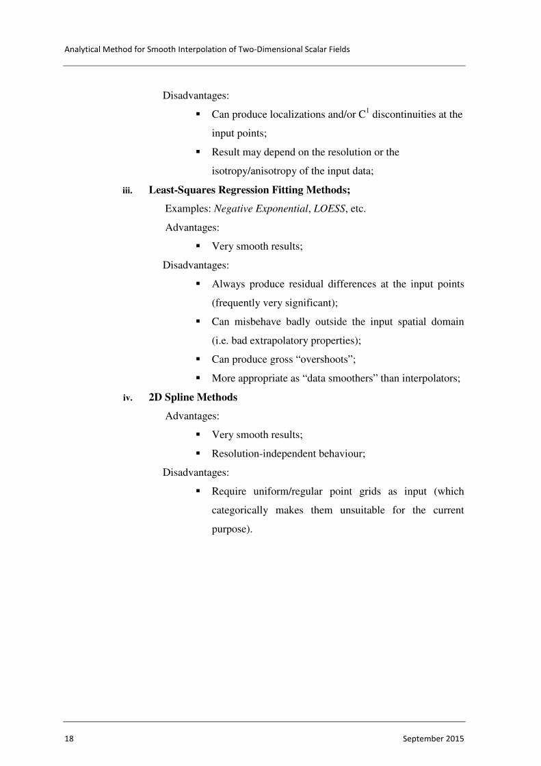
iii. Least-Squares Regression Fitting Methods;

Examples: Negative Exponential, LOESS, etc.

Advantages:

� Very smooth results;

Disadvantages:

� Always produce residual differences at the input points

(frequently very significant);

� Can misbehave badly outside the input spatial domain

(i.e. bad extrapolatory properties);

� Can produce gross “overshoots”;

� More appropriate as “data smoothers” than interpolators;

iv. 2D Spline Methods

Advantages:

� Very smooth results;

� Resolution-independent behaviour;

Disadvantages:

� Require uniform/regular point grids as input (which

categorically makes them unsuitable for the current

purpose).

REQUISITES AND KEY CONCEPTS


2. REQUISITES AND KEY CONCEPTS

2.1. Method Requisites

The method concept was defined in order to cumulatively satisfy – a priori –

the following requisites:

i. C0 continuity (mandatory);

ii. Zero residuals (i.e. zero difference at input points);

iii. Smooth (ideally, completely C1 continuous);

iv. Resolution-independent (i.e. consistent, regardless of resolution);

v. Anisotropy-insensitive (i.e. unaffected by fluctuations in input dataset

spatial distribution density);

vi. Low processing load (ideally O(n));

vii. Possibility of model manipulation and fine-tuning, but…

viii. Good “first results” (without fine-tuning).

2.2. Key Concepts

The above requisites led to the definition of the following concept guidelines:

i. Interpolation based on local trends (defined by means of tangency

planes at the input points);

ii. Local trends defined on vicinity criteria based on topological

relations (i.e. interconnected vertices in a triangular tessellation);

iii. Strictly local interpolation (avoiding the detrimental effects of

anisotropic spatial distributions and the exponential growth of

processing load with dataset size);

iv. Smoothness achieved by weighting based on smooth blending

functions (i.e. analytical simplicity);

v. Piecewise analytical method, allowing for virtually unlimited

interpolated mesh resolutions;


20 September 2015

ONE-DIMENSIONAL IMPLEMENTATION AND PROOF-OF-CONCEPT


3. ONE-DIMENSIONAL IMPLEMENTATION AND

PROOF-OF-CONCEPT

Before proceeding to the final implementation of the two-dimensional (2D)

method, a one-dimensional (1D) version of the idea was implemented. This worked as a

“proof-of-concept” and, additionally, allowed for a significant simplification of the

mathematical formulation for a first approach. In the context of the current paper, the 1D

implementation also allows for an easier explanation and introduction of the key concepts.

The final implementation will consist – fundamentally – in the generalization of the 1D

concept to a 2D spatial domain.

Figure 3.1 typifies the interpolation paradigm in one-dimensional space: the

interpolated curve contains the input points – i.e. zero residuals – and its gradient is locally

equal to the slope of the tangent lines Ti that define the local trends at the points (xi, f(xi)).

Figure 3.1. Illustration of the key-concepts of the method in a one-dimensional space.

Different criteria can be used to define the slope of the local trend tangents, as

long as they’re defined based on the values of neighbour points and how they relate to each

other (i.e. increasing or decreasing trend). For instance, the simplest criterion that can be

defined – and which works surprisingly well in practice – defines the tangent slope as the

f (x)

x xi xi+1 xi+2 xi-1 xi-2

Ti-1(x)

Ti (x)

Ti+1(x)


22 September 2015

gradient of the line segment that joins the two closest neighbour points (i.e. points

immediately before and after):

(3.1)

Alternatively, the tangent slope can be defined using an inverse distance

weighted least-squares linear regression of several neighbour points. Also, special cases

can (and should) be defined for notable points, such as the first and last point in the input

series and/or the points at the extrema.

The piecewise interpolated curve in a particular interval between two input

points – [xi, xi+1] – is defined by weighting the two adjacent tangents with a smooth

blending function (N) defined in the local coordinates of the interval (ξ):

(3.2)

Where:

ξ - Local coordinate in the interval;

N - Blending function (defined in the local domain);

Ti - Trend tangent line function at the point i (in global coordinates).

The blending function needs to be smooth (C1 continuous) and satisfy the

following conditions:

Specifically, its slope must be null at the local domain limits (i.e.: at ξ = 0 and

ξ = 1) and its value must be unitary at ξ = 0 and zero at ξ = 1.

Also, ideally, the sum of the weights should be equal to 1 or, at least,

approximately equal to 1:

Figures 3.2 and 3.3 show some examples of possible candidate blending

functions: the first is a sinusoidal function whilst the second is polynomial. Both have been

tried with good results. The difference between results with one or the other is negligible.



Figure 3.2. Example of a sinusoidal blending function.

Figure 3.3. Example of a polynomial blending function (3rd

degree).


24 September 2015

Other possible candidate for a blending function is the following 5th

degree

polynomial:

In fact, there’s a whole family of odd degree (greater than 1) polynomials with

integer coefficients that satisfies the basic conditions for a blending function. Polynomials

up to 7th

degree were tried for the current purpose, but no practical advantage was found

over the 3rd

degree polynomial or the sinusoidal blending function.

The expression (3.2) is algebraically so simple that it can be expanded in order

to gain some additional insight into its working principle.

The trend tangent lines can be written as:

(3.3)

And the local coordinates are calculated by:

(3.4)

Hence, the expansion of (3.1) – except for the blending function N – gives:

(3.5)

If the local trends are defined in their simplest form by expression (3.1) – i.e.

slope of the line that joins the previous and next input point in the series – then:

(3.6)

And, since the tangent line contains the point (xi, fi):

(3.7)



3.1. Demonstration of the C1 continuity

A short demonstration of the gradient continuity between the piecewise

segments of the interpolated curve is presented below.

The slope of the interpolated curve at the point (xi, f(xi)) can be obtained by

differentiating the expression (3.2):

(3.8)

Expanding by the product rule gives:

Taking into account the a priori conditions satisfied by the blending function:

We can easily simplify the previous expression and reach the conclusion that:

(3.9)

The gradient continuity of the interpolated piecewise function is, thus,

demonstrated.


26 September 2015

3.2. Controlling the Overshoots

With the previous presented definition of the method – in its one-dimensional

version – a very real practical problem may arise: if the slope of a trend tangent is very

high (in the limit, it can be almost infinite), the interpolation may overshoot significantly

outside the input range – i.e. it can give origin to values much higher than the maximum

input value and/or much lower than the minimum input value. This situation is illustrated

in Figure 3.4.

Figure 3.4. Illustration of an overshoot condition: the interpolated curve significantly exceeds the maximum

input value.

3.2.1. Solution

One possible solution for this problem – which was tested with very good

success – is to vary the tangent slopes along the local domain, i.e.: as a function of the

local coordinates. Figure 3.5 illustrates this concept.

f(x)

x x2 x3 x1

Max(fi)

x0 x4



Figure 3.5. Controlling an overshoot condition by continuously varying the slope of the trend tangent along

the local domain (i.e. as a function of the local coordinate).

In Figure 3.5, the variation of the slope of the trend tangent at the point i (Ti) is

shown as a function of the local coordinate ξ. At the point i (ξ = 0 and x = xi) there is no

change of slope (i.e. the tangent defines the local trend at the point). As the interpolation

evolves from the point i to the point i+1 the slope of the tangent decreases until its

minimum value (at ξ = 1 and x = xi+1), which is the slope of the line that joins both points i

and i+1. Conversely, the trend tangent at the point i+1 (not represented in the above graph)

evolves in a reciprocally equivalent manner.

As stated before, this method of overshoot control was implemented with very

good success. Its algebraic notation, however, is very difficult to formulate in an elegant

and non-obscure fashion. Hence, it will not be explicitly indicated in the current scope.

Note: Another approach for controlling overshoots is to purposely attenuate the tangent

slope at the global and local input extrema (i.e. maximum and minimum input

values). This allows some degree of freedom in fine-tuning the interpolation result.

f(x)

x x2 x3 x1

Max(fi)

x0 x4

Ti(ξ=0)

Ti(ξ=0.5)

Ti(ξ=1)


28 September 2015

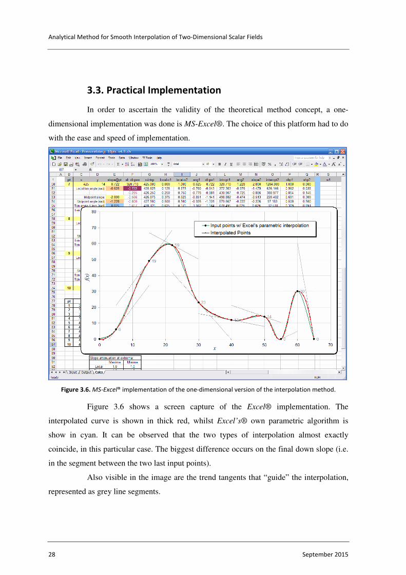
3.3. Practical Implementation

In order to ascertain the validity of the theoretical method concept, a one-

dimensional implementation was done is MS-Excel®. The choice of this platform had to do

with the ease and speed of implementation.

Figure 3.6. MS-Excel® implementation of the one-dimensional version of the interpolation method.

Figure 3.6 shows a screen capture of the Excel® implementation. The

interpolated curve is shown in thick red, whilst Excel’s® own parametric algorithm is

show in cyan. It can be observed that the two types of interpolation almost exactly

coincide, in this particular case. The biggest difference occurs on the final down slope (i.e.

in the segment between the two last input points).

Also visible in the image are the trend tangents that “guide” the interpolation,

represented as grey line segments.



Figure 3.7. Application – in MS-Excel® – for the interpolation of pressure histories – P(t) – from ten

experimental data points.

A practical application of the one-dimensional version of the method – also in

Excel® – is shown in Figure 3.7. In this particular case, the application is used to

interpolate pressure histories – P(t) – from ten metrology samples.

In this application, the user is given the option to choose one of several criteria

for the definition of the trends (i.e. tangents) at each input point, including inverse-distance

weighting (in the figure, the selected criterion is “average slope of all methods”).

The user is also given the freedom to manually attenuate the tangent slopes at

the global and local extrema, thus providing an extra means of controlling possible

overshoots.


30 September 2015

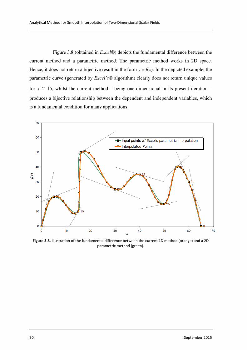
Figure 3.8 (obtained in Excel®) depicts the fundamental difference between the

current method and a parametric method. The parametric method works in 2D space.

Hence, it does not return a bijective result in the form y = f(x). In the depicted example, the

parametric curve (generated by Excel’s® algorithm) clearly does not return unique values

for x � 15, whilst the current method – being one-dimensional in its present iteration –

produces a bijective relationship between the dependent and independent variables, which

is a fundamental condition for many applications.

Figure 3.8. Illustration of the fundamental difference between the current 1D method (orange) and a 2D

parametric method (green).

TWO-DIMENSIONAL GENERALIZATION


4. TWO-DIMENSIONAL GENERALIZATION

In this chapter, the interpolation method previously defined for a one-

dimensional (1D) space will be generalized for two-dimensional (2D) space.

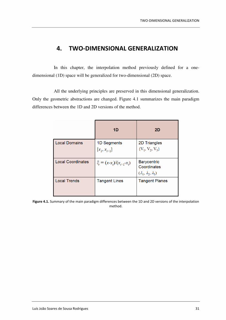
All the underlying principles are preserved in this dimensional generalization.

Only the geometric abstractions are changed. Figure 4.1 summarizes the main paradigm

differences between the 1D and 2D versions of the method.

Figure 4.1. Summary of the main paradigm differences between the 1D and 2D versions of the interpolation

method.


32 September 2015

4.1. Local Domains

In the 1D implementation, the local spatial domains were the linear intervals

between two contiguous input points (i.e. [xi, xi+1]). In 2D, the domains will have to be,

forcibly, 2D polygons.

The number of input points can be even or odd. This, in practice, forces the

choice of polygons to be 2D triangles (the simplest form of polygon).

Hence, the 2D implementation of the algorithm presupposes a prior subdivision

of the global data domain into triangular local domains. This can be achieved using a

triangular tessellation algorithm.

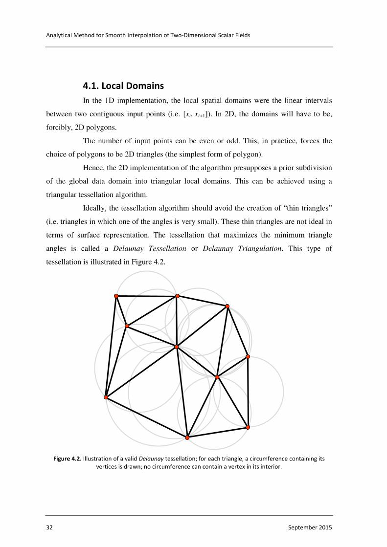
Ideally, the tessellation algorithm should avoid the creation of “thin triangles”

(i.e. triangles in which one of the angles is very small). These thin triangles are not ideal in

terms of surface representation. The tessellation that maximizes the minimum triangle

angles is called a Delaunay Tessellation or Delaunay Triangulation. This type of

tessellation is illustrated in Figure 4.2.

Figure 4.2. Illustration of a valid Delaunay tessellation; for each triangle, a circumference containing its

vertices is drawn; no circumference can contain a vertex in its interior.



As can be seen in Figure 4.2, a circumference was drawn for each triangle,

containing its vertices. In a valid Delaunay tessellation (which guarantees the

maximization of triangle angles), each circumference cannot contain any triangle vertex in

its interior.

4.2. Local Coordinate System

With local spatial domains established as 2D triangles, comes the need to

define an appropriate local coordinate system. The coordinate system should, ideally,

easily give us the relative distance to each of the triangle’s vertices, so that the weight of

the trend defined in each vertex in the final interpolated value can be easily calculated via a

blending function. The obvious choice is the Barycentric Coordinate System, usually

denoted by one of the following notations: (α, β, γ) or (λ1, λ2, λ3).

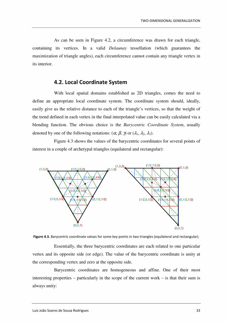
Figure 4.3 shows the values of the barycentric coordinates for several points of

interest in a couple of archetypal triangles (equilateral and rectangular):

Figure 4.3. Barycentric coordinate values for some key points in two triangles (equilateral and rectangular).

Essentially, the three barycentric coordinates are each related to one particular

vertex and its opposite side (or edge). The value of the barycentric coordinate is unity at

the corresponding vertex and zero at the opposite side.

Barycentric coordinates are homogeneous and affine. One of their most

interesting properties – particularly in the scope of the current work – is that their sum is

always unity:

(1,0,0)

(0,0,1)

(0,1,0) (1/2,1/2,0)

(1/2,0,1/2) (0,1/2,1/2)

(1/2,1/4,1/4) (1/4,1/2,1/4)

(1/4,1/4,1/2)

(1/3,1/3,1/3)

(0,0,1)

(0,1,0) (1/2,1/2,0) (1,0,0)

(1/2,0,1/2) (0,1/2,1/2)

(1/2,1/4,1/4) (1/4,1/2,1/4)

(1/4,1/4,1/2)

(1/3,1/3,1/3)


34 September 2015

(4.1)

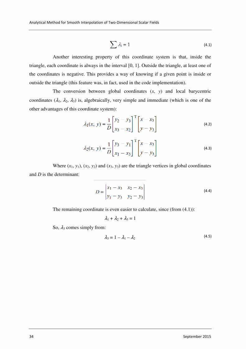
Another interesting property of this coordinate system is that, inside the

triangle, each coordinate is always in the interval [0, 1]. Outside the triangle, at least one of

the coordinates is negative. This provides a way of knowing if a given point is inside or

outside the triangle (this feature was, in fact, used in the code implementation).

The conversion between global coordinates (x, y) and local barycentric

coordinates (λ1, λ2, λ3) is, algebraically, very simple and immediate (which is one of the

other advantages of this coordinate system):

(4.2)

(4.3)

Where (x1, y1), (x2, y2) and (x3, y3) are the triangle vertices in global coordinates

and D is the determinant:

(4.4)

The remaining coordinate is even easier to calculate, since (from (4.1)):

λ1 + λ2 + λ3 = 1

So, λ3 comes simply from:

λ3 = 1 – λ1 – λ2 (4.5)



4.3. Local Trends

In the one-dimensional implementation, the interpolated function trend at the

input points is defined via a tangent line. The equivalent geometric abstraction in 2D is a

tangent plane.

In 1D, the slope of the tangent line was defined by the neighbour points (e.g.

the slope of a line segment joining the previous and next point in the series). In 2D, the

gradient of the tangency plane will also be calculated from the values of neighbour points.

However, in this case, finding the neighbour points is not as straightforward as in 1D.

Fortunately, the triangular tessellation (necessary for the establishment of local domains)

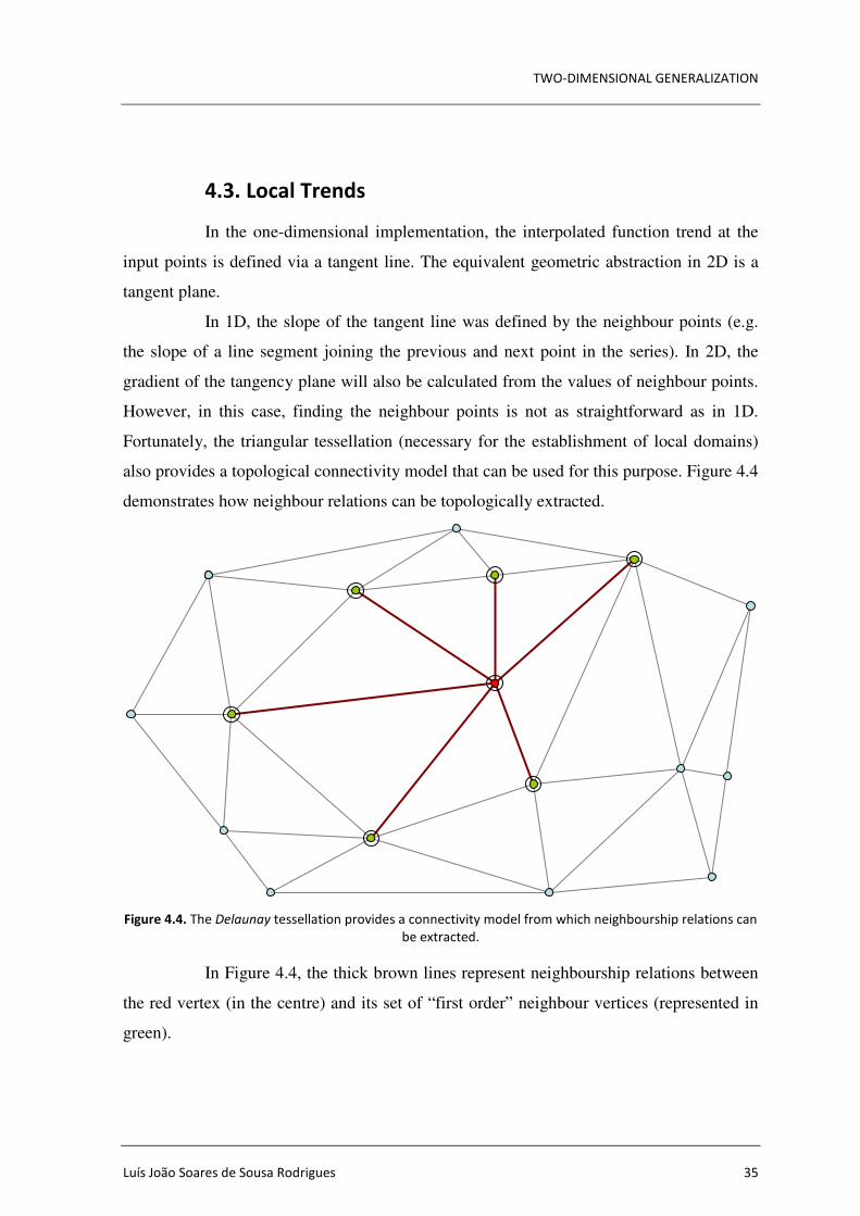
also provides a topological connectivity model that can be used for this purpose. Figure 4.4

demonstrates how neighbour relations can be topologically extracted.

Figure 4.4. The Delaunay tessellation provides a connectivity model from which neighbourship relations can

be extracted.

In Figure 4.4, the thick brown lines represent neighbourship relations between

the red vertex (in the centre) and its set of “first order” neighbour vertices (represented in

green).


36 September 2015

In an analogous manner to the 1D method, the gradient of the tangency plane

that defines the local trend at a given input point can be calculated via a least-squares

regression using the neighbour vertices.

The plane that best fits the neighbour points (xi, yi, fi) of vertex V can be

calculated by solving the following linear system [8]:

(4.6)

If the neighbour vertices (xi, yi, fi) of vertex V are linearly independent (e.g. not

collinear – which is inherently assured in the current application), the system has an

immediate solution (e.g., by applying Cramer’s Rule). The gradient components of the

tangency plane are, thus, given by:

(4.7)

(4.8)

Where D is the determinant:

(4.9)

Since the plane has to include the vertex V = (xV, yV, fV), the following

translation must be applied:

(4.10)

TWO-DIMENSIONAL METHOD DEFINITION


5. TWO-DIMENSIONAL METHOD DEFINITION

In the previously presented 1D simplified version of the method, the

interpolated curve was obtained by weighing the two trend tangent lines – that contain the

data points that define the limits of the local domain – using one-dimensional blending

functions working in local linear coordinates.

In an analogous fashion, the 2D interpolated surface/field is obtained by

weighing – within each local domain (i.e. triangle) – the three trend planes defined (in the

manner explained in the previous section) at each input data point (or mesh vertex). The

blending functions are kept one-dimensional, but now work with barycentric coordinates.

The piecewise interpolated surface is defined (for each local domain) by the

following expression:

(5.1)

Where:

PVi - Tangent plane function that defines the surface trend at the vertex Vi

(defined in the global coordinate system XY);

λi - Local barycentric coordinate in relation to the vertex Vi;

N - One-dimensional blending function defined in the local domain

(barycentric coordinate system);

In order to make it less abstract, the plane functions can be expanded (with

some loss in elegance):

(5.2)


38 September 2015

METHOD IMPLEMENTATION


6. METHOD IMPLEMENTATION

6.1. General Workflow

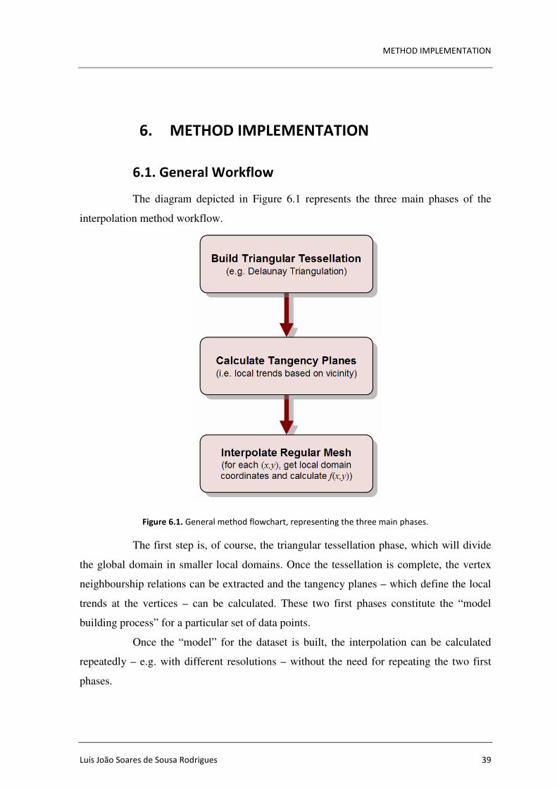
The diagram depicted in Figure 6.1 represents the three main phases of the

interpolation method workflow.

Figure 6.1. General method flowchart, representing the three main phases.

The first step is, of course, the triangular tessellation phase, which will divide

the global domain in smaller local domains. Once the tessellation is complete, the vertex

neighbourship relations can be extracted and the tangency planes – which define the local

trends at the vertices – can be calculated. These two first phases constitute the “model

building process” for a particular set of data points.

Once the “model” for the dataset is built, the interpolation can be calculated

repeatedly – e.g. with different resolutions – without the need for repeating the two first

phases.


40 September 2015

6.2. Implementation Platform

The method prototype was coded in Visual Basic 6.0 ®. The main reasons for

the selection of this implementation platform were:

� A license was readily available;

� It’s an interpreted language, which speeds up development and

debugging (e.g. it’s easy to interrupt execution and execute commands at

a line prompt);

� It’s a structured language;

� Implements an object-oriented paradigm;

� Supports complex data structures;

� Includes a good integrated development environment (IDE) – Microsoft

Visual Studio® – including interactive code and graphical user interface

(GUI) editors;

� Good support documentation;

� Relatively recent working experience with it.

On the downside, this platform revealed the following disadvantages:

� Slow execution speed (although good enough for the current purpose,

i.e.: rapid prototyping);

� Graphical display object with very limited functionality and very poor

performance;

These shortcomings, however, were found no to hinder the implementation in a

significant manner and were largely superseded by the advantages.

METHOD IMPLEMENTATION


6.3. Delaunay Tessellation Algorithm

Among the several existent algorithms for building a Delaunay tessellation [9-

14], a brief bibliographical research led to the selection of the method described by

Bowyer [13] and Watson [14] (appropriately known as the Bowyer-Watson Algorithm).

This algorithm is relatively simple to understand and implement and is also very efficient.

Another reason for its selection is related to the fact that it’s relatively easy to find open

source code for it in the public domain.

A detailed description of this algorithm is beyond the scope of the current

paper (it can be found in the given references). Nevertheless, a pseudo-code is reproduced

below, in order to provide a topical idea about its principles.

function BowyerWatson (pointList)

// pointList is a set of coordinates defining

// the points to be triangulated

triangulation := empty triangle mesh data structure

add super-triangle to triangulation

// The “super-triangle” encompasses all the input points

for each point in pointList do

// add all the points one at a time to the triangulation

badTriangles := empty set

for each triangle in triangulation do

// first find all the triangles that are no longer valid due to

// the insertion

if point is inside circumcircle of triangle

add triangle to badTriangles

polygon := empty set

for each triangle in badTriangles do

// find the boundary of the polygonal hole

for each edge in triangle do

if edge is not shared by any other triangles in badTriangles

add edge to polygon

for each triangle in badTriangles do

// remove them from the data structure

remove triangle from triangulation

for each edge in polygon do

// re-triangulate the polygonal hole

newTri := form a triangle from edge to point

add newTri to triangulation

for each triangle in triangulation

// done inserting points, now clean up

if triangle contains a vertex from original super-triangle

remove triangle from triangulation

return triangulation


42 September 2015

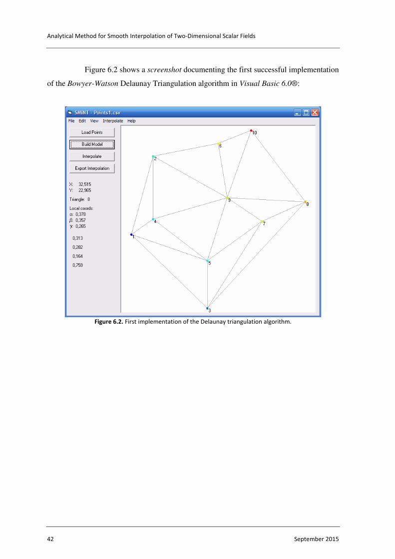
Figure 6.2 shows a screenshot documenting the first successful implementation

of the Bowyer-Watson Delaunay Triangulation algorithm in Visual Basic 6.0®:

Figure 6.2. First implementation of the Delaunay triangulation algorithm.

FIRST RESULTS


7. FIRST RESULTS

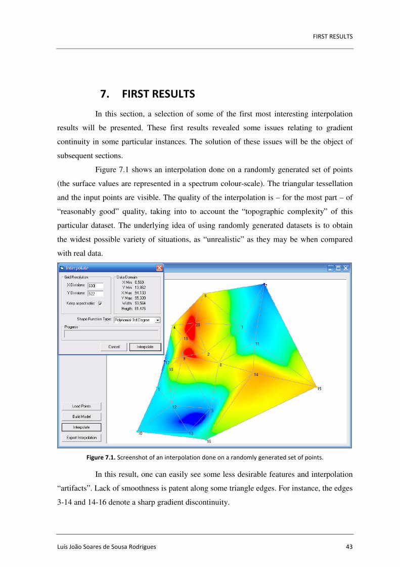
In this section, a selection of some of the first most interesting interpolation

results will be presented. These first results revealed some issues relating to gradient

continuity in some particular instances. The solution of these issues will be the object of

subsequent sections.

Figure 7.1 shows an interpolation done on a randomly generated set of points

(the surface values are represented in a spectrum colour-scale). The triangular tessellation

and the input points are visible. The quality of the interpolation is – for the most part – of

“reasonably good” quality, taking into to account the “topographic complexity” of this

particular dataset. The underlying idea of using randomly generated datasets is to obtain

the widest possible variety of situations, as “unrealistic” as they may be when compared

with real data.

Figure 7.1. Screenshot of an interpolation done on a randomly generated set of points.

In this result, one can easily see some less desirable features and interpolation

“artifacts”. Lack of smoothness is patent along some triangle edges. For instance, the edges

3-14 and 14-16 denote a sharp gradient discontinuity.


44 September 2015

Figure 7.2 is a representation of the same interpolation in 3D perspective with

values represented as colour “isobands” (obtained with the software Graphis®):

Figure 7.2. 3D perspective of an interpolation done on a randomly generated set of points.

Although this representation is still far from ideal, it still makes the gradient

discontinuities more apparent. These discontinuities occur mainly on the edges of very

“thin” triangles, which, ideally, should not exist.

In order to get an interpolation behaviour more akin to what one would get

with real data, a “field simulant” dataset was manually created. Figure 7.3 and Figure 7.4

document the results.

FIRST RESULTS


Figure 7.3. Interpolation of a manually created “realistic” field.

Figure 7.4 shows the interpolation result with contour lines (obtained in

SigmaPlot®).

Figure 7.4. Contoured representation of an interpolation of a simulated “realistic” field.

The contour lines allow a better assessment of the quality of the interpolation.

In this particular case, most of the interpolation is very smooth and of general good quality.

The notable exceptions are the gradient discontinuities near the bottom corners of the field,

which are caused (again) by thin triangles in the underlying tessellation.

Next, the first results of the application of the interpolation method to real

datasets will be shown and analysed.


46 September 2015

Figure 7.5 shows an interpolation done over an actual empirically obtained

dataset. The scalar field represents the arrival instants (in nanoseconds) of a shockwave

front at different probes (in this case, optical fibres) embedded in an inert medium

(PMMA, in this case).

Figure 7.5. Interpolation done over an actual metrology dataset; scalar value represents shockwave arrival

time.

In Figure 7.6, the same result is represented in 3D perspective with the scalar

value (time in ns) represented as contoured colour bands:

Figure 7.6. 3D perspective of an interpolated field, done over an actual metrology dataset; the scalar value

(represented in colour isobands) represents shockwave arrival time.

The field interpolation quality is, qualitatively, adequate. Some gradient

discontinuities are apparent in the upper right region of the field, due to the underlying thin

triangles of the Delaunay tessellation.

IMPROVING THE GRADIENT CONTINUITY


8. IMPROVING THE GRADIENT CONTINUITY

The evaluation of the first results denoted the occurrence of sharp gradient

discontinuities along the edges of “thin” triangles. Ideally, the occurrence of these thin

triangles should be avoided by adding extra points to the model (this subject will be treated

in the chapter dedicated to extrapolation and data densification).

Nevertheless, another approach for solving this issue is to “attack” its root

cause: as it is defined in Chapters 4 and 5, the method is not C1 continuous along the

triangular domain boundaries (it is, however, C1 continuous in every other location,

including the input data points).

The reason for the gradient discontinuity along the triangle edges lies in the

definition of the local coordinate systems: their orientation (in relation to the global

system) changes abruptly in the transition from one local domain to another.

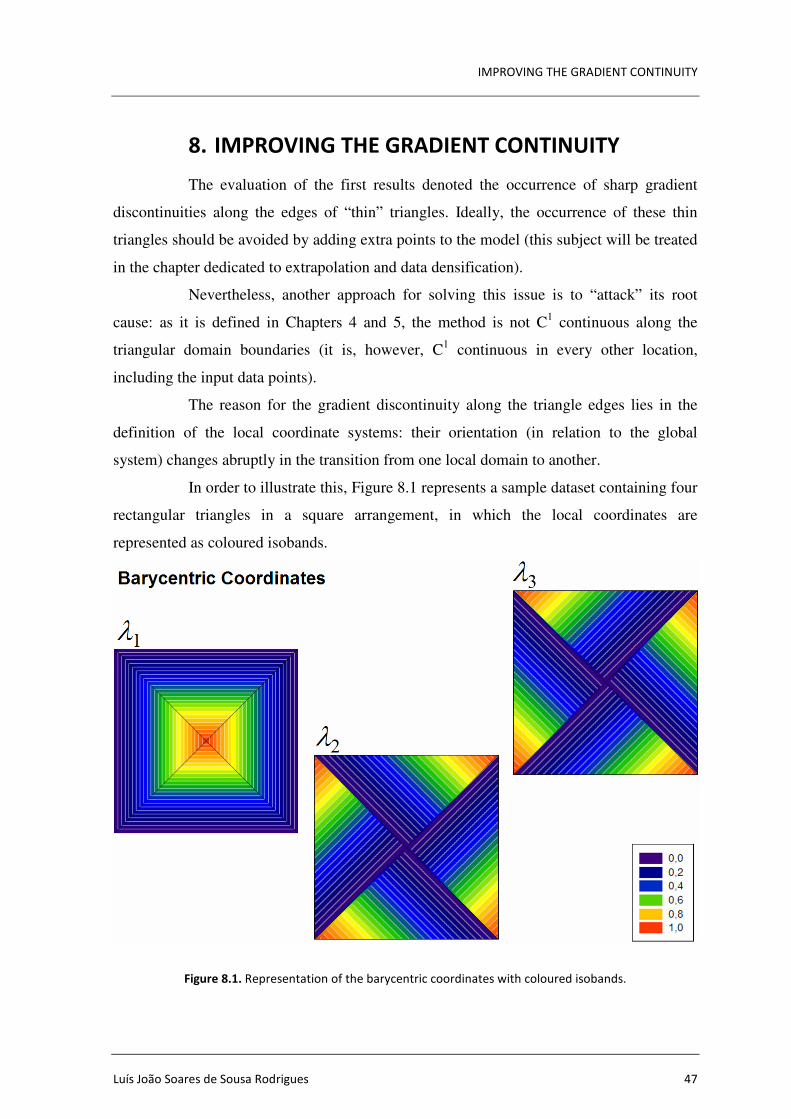
In order to illustrate this, Figure 8.1 represents a sample dataset containing four

rectangular triangles in a square arrangement, in which the local coordinates are

represented as coloured isobands.

Figure 8.1. Representation of the barycentric coordinates with coloured isobands.


48 September 2015

By examining the spatial evolution of, for instance, the local barycentric

coordinate λ1, one can see that its metric orientation changes abruptly (90º, in this case)

between each adjacent triangle. It’s this abrupt metric rotation that, ultimately, causes

gradient discontinuities in the interpolation, particularly in the case of very thin triangles.

Next, some possible solution approaches for this problem will be addressed.

8.1. Edge-Orthogonal Local Coordinates

The first approach to solve the lack of gradient continuity of the interpolation

method is to orthogonalize the local coordinates in relation to the triangle edges. Figure 8.2

attempts to illustrate this principle.

Figure 8.2. Representation of the concept of the “edge-orthogonal coordinates”.

Here, the barycentric coordinate λ1 was replaced by its “edge-orthogonal”

counterpart ω1. The green isolines represent different values of ω1. Focusing on the ω1 =

1/2 isoline, we can see that it is locally orthogonal with the triangle sides V1V2 and V1V3.

and intersects them exactly at the midpoint. Hence, it must take a curved shape.

Of course, this operation cannot be done for the entirety of the triangle area, as

is demonstrated by the isoline ω1 = 0. In order to maintain the orthogonality with the

V1

V2

V3

ω1 = 0

ω1 = 1/2

ω1 = 1



triangle sides, this isoline overshoots and undershoots the side V2V3. Thus, the

orthogonalization operation should “fade out” as it approaches the opposite side (V2V3 in

this case) to avoid this undesirable behaviour. Near the opposite side, the local coordinates

become purely barycentric.

Algebraically, the edge-orthogonal coordinates can be defined as a function of

the barycentric coordinates, by the following expressions:

(8.1)

(8.2)

(8.3)

Where N is the already familiar one-dimensional blending function (applied

here in a completely different context). P is the point – defined in real world coordinates –

for which we want to calculate the edge-orthogonal local coordinates.

The right vector elements are the ratios between the distance of the point P to

the vertex of origin of the coordinate we want to calculate (V1 for the coordinate ω1, V2 for

the coordinate ω2…) and the length of the adjacent triangle sides (all defined in global

coordinates).

Note that the above expressions do not contain the previously mentioned “fade

out” transition to barycentric coordinates near the opposite triangle edge (to avoid

undershoots and overshoots), for notation clarity reasons.


50 September 2015

Figure 8.3. Representation of the edge-orthogonal coordinates with coloured isobands.

Figure 8.3 represents this coordinate system transformation. Note that all

coordinate isolines form, locally, a 90º angle with the triangle sides. In the case of ω1, the

result is concentric perfectly circular isolines (when a sinusoidal blending function is

used). The “fade to barycentric” transition is visible near the outer edges.

Next, the impact of using edge-orthogonal coordinates will be examined on

some interpolation results.

In Figure 8.4, a very simple model (basically four pyramids) is used to show a

comparison between a linear interpolation (in order to visualize the underlying model), an

interpolation using barycentric coordinates for the blending functions and an interpolation

using edge-orthogonal coordinates.



Figure 8.4. Interpolation comparison – using a simplistic model – between the use of barycentric

coordinates and the use of edge-orthogonal coordinates.

In the case of the barycentric coordinates (Figure 8.4, centre), sharp edges –

denoting gradient discontinuities – are clearly visible. By using edge-orthogonal

coordinates (Figure 8.4, right), the gradient discontinuities completely disappear. The

advantage of using edge-orthogonal local coordinates for the blending functions is, thus,

clearly apparent.

Now, the impact of using edge-orthogonal coordinates on a more realistic

situation will be analysed. For this purpose, the simulated field dataset will be used. Figure

8.5 documents the comparison between an interpolation done with barycentric coordinates

(top) and an interpolation using edge-orthogonal coordinates (bottom).


52 September 2015

Figure 8.5. Comparison between an interpolation using barycentric coordinates (top) and an interpolation

using edge-orthogonal coordinates (bottom).

The differences between the two results are quite clear: the gradient

discontinuity near the bottom corners improved considerably with the use of edge-

orthogonal coordinates.

Unfortunately, an undesirable “side-effect” of using edge-orthogonal

coordinates is also visible: by forcing the coordinates to a 90º angle with the triangle sides,

extra spurious surface inflections are introduced (mainly visible at the bottom of the above

figure).



8.2. Edge-Continuous Local Coordinates

Previously, an undesirable side-effect of using edge-orthogonal coordinates

was observed: by forcing the coordinates to be orthogonal with the triangle edges, spurious

inflections were introduced into the interpolated surface.

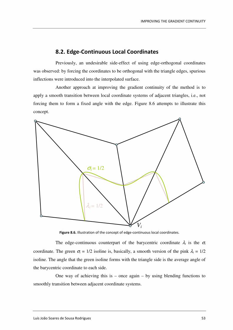
Another approach at improving the gradient continuity of the method is to

apply a smooth transition between local coordinate systems of adjacent triangles, i.e., not

forcing them to form a fixed angle with the edge. Figure 8.6 attempts to illustrate this

concept.

Figure 8.6. Illustration of the concept of edge-continuous local coordinates.

The edge-continuous counterpart of the barycentric coordinate λi is the σi

coordinate. The green σi = 1/2 isoline is, basically, a smooth version of the pink λi = 1/2

isoline. The angle that the green isoline forms with the triangle side is the average angle of

the barycentric coordinate to each side.

One way of achieving this is – once again – by using blending functions to

smoothly transition between adjacent coordinate systems.

Vi

λi = 1/2

σi = 1/2


54 September 2015

This, however, is not easily done and – so far – an elegant formulation for this

process was not achieved. Figure 8.7 illustrates the best attempt at achieving a smooth

transition between adjacent local coordinate systems.

Figure 8.7. Representation of the edge-continuous coordinates with coloured isobands.

As can be observed for the σ1 coordinate, the result of the current attempt is

still far from perfect. The curvature of the isolines denotes some undesirable undulations.

Still, this crude attempt was tested with the same datasets used for testing the

edge-orthogonal datasets, for direct comparison.



Figure 8.8. Interpolation comparison – using a simplistic model – between the use of barycentric, edge-

orthogonal and edge-continuous coordinates.

The difference between the interpolations done with edge-orthogonal and edge-

continuous coordinates is hardly discernible in this example. Both results look good, with

no visible gradient discontinuities. In order to better evaluate the differences, Figure 8.9

presents a top view with contour lines.

Figure 8.9. Top view of the interpolation comparison between the use of edge-orthogonal and edge-

continuous coordinates.


56 September 2015

There is, in fact a slight morphological difference. But, qualitatively, both

versions are equivalent in this particular case. A comparison using a more realistic dataset

can be more useful, as illustrated in Figure 8.10.

Figure 8.10. Comparison between an interpolation using edge-orthogonal coordinates (top) and an

interpolation using edge-continuous coordinates (bottom).

The differences are slight but somewhat important. With the edge-continuous

coordinates, there are less spurious surface inflections (and less pronounced), as expected.

Unfortunately, the interpolated solution at the very thin triangles in the bottom

corners reveals an undesirable behaviour.

Clearly, the approach of smoothly transitioning between local coordinate

systems works well. But a better method of doing it is needed. There is still much room for

improvement in this respect.

DATA DENSIFICATION AND EXTRAPOLATION


9. DATA DENSIFICATION AND EXTRAPOLATION

As defined in the objectives, the method must include good extrapolatory

capabilities. This is most useful when, for instance, a rectangular interpolated field/surface

must be produced from a scattered set of points which do not configure a rectangle.

Also, another very useful functionality is the possibility of increasing the

number of vertices in the model, in order to avoid the undesirable “thin triangles”.

A unique solution was found that addresses both necessities – i.e. data

densification and extrapolation – via the same mechanism: a provision for adding dataless

points (i.e. points with 2D position but no scalar value) to the dataset and an algorithm for

automatic estimation of the values of these extra points, based on the same trend paradigm

that is the foundation of the interpolation method.

9.1. Extrapolation/Densification Algorithm

The implemented extrapolation/densification algorithm relies on the same basic

philosophy of the final interpolation method: the extrapolated/interpolated value at the

additional dataless points is estimated based on the field/surface trend (i.e. tangency plane)

at the nearest connected neighbours. The final value results from an inverse distance

weighted convex (linear) combination.

The extrapolation algorithm is iterative: dataless nodes that have the greatest

number of neighbours with data (i.e. input points) are treated first. Then, the extrapolation

“propagates” from the “data rich” regions to the dataless regions in a stepwise fashion.

Between each extrapolation step, the tangent planes that define the local trend are

recalculated. Although this approach results in a relatively heavy processing load, it

ensures that the extrapolation is smooth and that the slope of the extrapolated regions

remains coherent with the gradient trends defined by the input data set.


58 September 2015

The pseudo-code below outlines the high-level iteration of the algorithm:

PointSet := LoadFromFile(File)

FieldModel := Triangulate(PointSet)

DatalessPointsCount := CountDatalessPoints(FieldModel)

RequiredNumberOfDatumNeighbors := 4

While DatalessPointsCount > 0

CalculateTangencyPlanes(FieldModel)


DatalessPointsBeforeExtrapolation := DatalessPointsCount

Extrapolate(FieldModel, RequiredNumberOfDatumNeighbors)


If DatalessPointsCount = DatalessPointsBeforeExtrapolation

Decrement RequiredNumberOfDatumNeighbors

EndIf

Loop

CalculateTangencyPlanes(FieldModel)

9.2. Testing the Extrapolation/Densification Algorithm

The extrapolation/densification algorithm was tested with a real dataset,

resulting from an experiment designed to resolve a cross-section of the shock field inside

an inert polymer – PMMA in this case (this dataset has already been presented before). The

data points are spatially characterized in the XY plane and contain the instant of interaction

of a shockwave with a bundle of PMMA optical fibres. The original dataset containing 70

× (xi, yi, ti) points is shown in Figure 9.1 (from an actual screenshot taken from the

interpolator application) colour coded by value (t in [ns]) from lower (blue) to higher (red).

Figure 9.1. Actual empirical dataset containing 70 points, colour coded by value (in this case, time in [ns])

from lower (blue) to higher (red).



As we can see, the dataset is “quasi-structured” in terms of spatial distribution,

but presents a very irregular outline and has some “holes” or unpopulated regions (the data

from those regions was irretrievable from the experimental record). Figure 9.2 depicts a

shaded 3D perspective of the input data, resulting from a linear interpolation based on a

Delaunay triangulation.

Figure 9.2. Colour isoband 3D perspective of the input data, resulting from a linear interpolation based on a

Delaunay triangulation.

The surface gradient discontinuities are apparent (although the figure

resolution is not ideal for a detailed examination), as well as the irregular outline. In order

to obtain a rectangular domain and “fill-in” the dataless regions, a mesh of additional

dataless points was added to the original dataset (resulting in a total of 139 points). Figure

9.3 documents the total mesh (dataless nodes are represented as white circles).

Figure 9.3. Input dataset mesh for extrapolation/densification; white (hollow) points contain no data; actual

data points are represented in dark blue.


60 September 2015

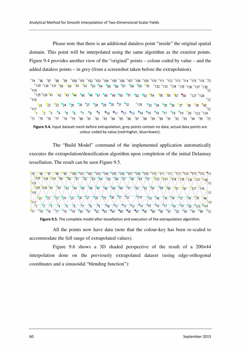
Please note that there is an additional dataless point “inside” the original spatial

domain. This point will be interpolated using the same algorithm as the exterior points.

Figure 9.4 provides another view of the “original” points – colour coded by value – and the

added dataless points – in grey (from a screenshot taken before the extrapolation).

Figure 9.4. Input dataset mesh before extrapolation; grey points contain no data; actual data points are

colour coded by value (red=higher, blue=lower).

The “Build Model” command of the implemented application automatically

executes the extrapolation/densification algorithm upon completion of the initial Delaunay

tessellation. The result can be seen Figure 9.5.

Figure 9.5. The complete model after tessellation and execution of the extrapolation algorithm.

All the points now have data (note that the colour-key has been re-scaled to

accommodate the full range of extrapolated values).

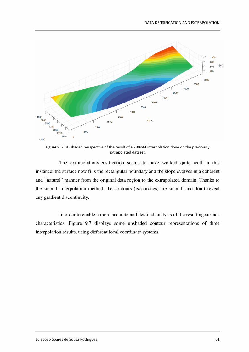
Figure 9.6 shows a 3D shaded perspective of the result of a 200×44

interpolation done on the previously extrapolated dataset (using edge-orthogonal

coordinates and a sinusoidal “blending function”):



Figure 9.6. 3D shaded perspective of the result of a 200×44 interpolation done on the previously

extrapolated dataset.

The extrapolation/densification seems to have worked quite well in this

instance: the surface now fills the rectangular boundary and the slope evolves in a coherent

and “natural” manner from the original data region to the extrapolated domain. Thanks to

the smooth interpolation method, the contours (isochrones) are smooth and don’t reveal

any gradient discontinuity.

In order to enable a more accurate and detailed analysis of the resulting surface

characteristics, Figure 9.7 displays some unshaded contour representations of three

interpolation results, using different local coordinate systems.


62 September 2015

Barycentric local coordinates

Edge-continuous local coordinates

Edge-orthogonal local coordinates

Figure 9.7. Comparison of contour representations of interpolation results using three different types of

local coordinates.

The differences between the versions obtained with different local coordinate

systems are minimal and very hard to pinpoint, at least for this particular dataset and

interpolation resolution.

CONCLUSIONS


10. CONCLUSIONS

The method concept was demonstrated as viable and fulfilled all the requisites

stated a priori. Nevertheless, there is still much room for improvement. Some results

revealed some shortcomings of the method for some particular types of data distributions.

Further efforts should be applied in the refinement of the local coordinate

systems – namely the smooth transition between adjacent local domains – since this seems

to be the most promising avenue for improving the gradient continuity and the overall

smoothness of the results.

The quality of the interpolation may also be further enhanced by refining the

tessellation algorithm. For instance, the implementation of a constrained Delaunay

triangulation could allow some degree of human intervention on the tessellation topology.

Other possibility would be the implementation of a 3D tessellation algorithm or, at least,

some form of taking into account the value (or third dimension) for determining the best

tessellation solution (which does not necessarily obey the Delaunay criterion).

Other useful functionalities could also be added to the implemented software,

e.g.: definition of convex hulls (in order to contain the triangulation within a given

perimeter), data and model editing capabilities, further parameter manipulation, etc.

The current method is not necessarily “better” than other methods. No

interpolation method is “perfect” or perfectly suitable for all applications and dataset

characteristics. All depends on the nature of the data at hand.

An extensive comparative study with other interpolation methods is essential

for correctly ascertaining the relative qualities and shortcomings of the current method.

Such a study was initially intended in the scope of the current work but – due to time

constraints – could not be accomplished.

Notwithstanding, the author hopes that the current work might be of relevance

and that this method might, after some refinements, make part of the arsenal of algorithms

used by scientists and engineers faced with the not so straightforward challenge of

achieving good quality and realistic field and surface representations with less than perfect

source data.


64 September 2015

BIBLIOGRAPHY


BIBLIOGRAPHY

[1] De Berg, M., Cheong, O., Van Kreveld, M., Overmars, M. (2008), “Computational

Geometry: Algorithms and Applications”, 3rd

Edition, Springer-Verlag, Berlin.

[2] Yang, Ch., Kao, S., Lee, F., Hung, P. (2004), “Twelve Different Interpolation

methods: A Case Study of Surfer 8.0”, Geo-Imagery Bridging Continents, XXth

ISPRS Congress.

[3] Bajaj, C., (1988) “Geometric Modelling with Algebraic Surfaces”, The

Mathematics of Surfaces, III ed., D. Handscomb, Oxford University Press, pp. 3 -

48.

[4] Mayer, T.H. (2004), “The Discontinuous Nature of Kriging Interpolation for

Digital Terrain Model”, Cartography and Geographic Information Science, Volume

31, Number 4, pp. 209-216.

[5] Smith, W.H.F., Wessel, P. (1990) “Gridding with continuous curvature splines in

tension”, Geophysics, Vol. 55, Nº 3, pp. 293-305.

[6] Sibson, R. (1981) “A brief description of natural neighbor interpolation (Chapter

2)”, In V. Barnett, Interpreting Multivariate Data, John Wiley, pp. 21–36.

[7] Sukumar, N., (1997) “A Note on Natural Neighbor Interpolation and the Natural

Element Method (NEM)”, Theoretical and Applied Mechanics, Northwestern

University.

[8] Leon, S.J. (1990), “Linear Algebra With Applications”, 3rd

Edition, Macmillan.

[9] Van Kreveld, M. (2006), “Algorithms for Triangulated Terrains”, Dept. of

Computer Science, Utrecht University, The Netherlands.

[10] Lee, D.T., Schachter, B.J. (1980), “Two Algorithms for Constructing a Delaunay

Triangulation”, International Journal of Computer and Information Sciences, Vol.

9, nº 3, pp. 219-242.

[11] Liu, Y., Snoeyink, J, (2005) “A comparison of five implementations of 3D

Delaunay tessellation”, Combinatorial and Computational Geometry nº 52, pp. 439-

458.

[12] Bourke, P. (1989), “Efficient Triangulation Algorithm Suitable for Terrain

Modelling or An Algorithm for Interpolating Irregularly-Spaced Data with

Applications in Terrain Modelling”, Pan Pacific Computer Conference, Beijing,

China.

[13] Bowyer, A. (1981), “Computing Dirichlet tessellations”, The Computer Journal nº

24, pp. 162–166.

[14] Watson, D.F. (1981), “Computing the n-dimensional Delaunay tessellation with

application to Voronoi polytopes”. The Computer Journal nº 24, pp. 167–172.


66 September 2015

analytical method for smooth interpolation of two-dimensional … · departamento de engenharia...

Documents