analytical method for designing flexible foundations · pdf fileanalytical method for...

A R C H I W U M I N S T Y T U T U I N Ż Y N I E R I I L Ą D O W E J

Nr 23 ARCHIVES OF INSTITUTE OF CIVIL ENGINEERING 2017

ANALYTICAL METHOD FOR DESIGNING FLEXIBLE FOUNDATIONS

FOR SOIL-STEEL COMPOSITE STRUCTURES1

Wojciech SAMOLEWSKI* *) MSc. Eng., ViaCon Construction Sp. z o.o., Rydzyna, Poland

Soil-steel composite structures are usually designed with the use of analytical meth-ods presented in such standards as SDM, CHBDC, or ASHTOO. Nevertheless, none of those standards introduces an analytical method for designing flexible foundations. Therefore, such foundations are usually designed with the use of time consuming and labor intensive full FEM analysis.

In this paper the author makes an attempt at using classical foundations engineering solutions and models a corrugated steel plate foundation as an elastic beam on Winkler foundation. Moreover, he tries to find a method that takes into account layered configu-rations of geological substrates.

Subsequently, the obtained values are compared against corresponding FEM analy-sis results. Likewise, the author evaluates the usefulness and accuracy of the presented computational approach.

Key words: flexible foundation, elastic beam, Winkler foundation, soil-steel composite structure.

1. INTRODUCTION

In today’s world, bridge engineering requires quick and efficient concept verification methods. There is no time for labor consuming calculations at the initial concept stage. On the other hand, no matter how preliminary the concept is, there is no room for grave mistakes since they can lead to an economic disas-ter.

A response to the need for quick and efficient methods in the design of soil-steel composite structures is provided by analytical computation methods pre-sented in such standards as SDM, CHBDC or ASHTOO. These methods can easily be implemented in widely available computer software such as Microsoft Excel or PTC Mathcad. Unfortunately, none of the standards listed above pro-vides an analytical method for designing flexible foundations.

1 DOI 10.21008/j.1897-4007.2017.23.23

252 Wojciech Samolewski

Implementation of corrugated steel plate foundations is one of the most common ideas on structure cost optimization. However, the range of their ap-plicability is limited by numerous factors. The idea usually comes unexpectedly and the answer is needed immediately. Therefore, a quick method to verify the idea’s feasibility is also necessary.

2. FORCES ACTING ON THE FOUNDATION

In the analytical methods for soil-steel composite structures design it is usu-ally assumed that the normal force value is constant around the profile perimeter. Moreover, it is usually assumed that the shear force value is negligibly low. Numerous field tests and FEM analyses have confirmed that these assumptions are not exaggerated. What is more, they lead to the conclusion that flexible steel structures act on the foundations only with forces directed tangentially to their profiles’ curvatures at the level of support.

Figure 1. Forces acting in different directions depending on the profile's curvature

2.1. Vertical forces

Concluding from the above, the vertical force for foundation design (Vd) can be calculated as the vertical component of the design normal force in structure (Fd). But what value of that force should be taken into consideration?

In the structural design methods the most unfavorably loaded cross sections of the steel shell are usually sought. Using normal force values calculated with this approach, simply multiplied by the foundation length, leads to a solution with a considerable safety margin. Characteristic normal force values in an ex-ample structure obtained with different calculation methods are listed below together with analogical field test results.

Analytical method for designing flexible foundations for soil-steel … 253

Table 1. Normal force values in an example structure calculated in accordance with different methods (Nk,soil – normal force induced by backfill, Nk,traffic – normal force induced by traffic load)

Data source Nk,soil

[kN/m] Nk,traffic

[kN/m] Nk

[kN/m] 1 SDM – structural design 31.22 80.47 111.69 2 SDM + ASHTOO reduction 31.22 21.46 52.68 3 ASHTOO 21.92 27.03 48.95 4 PLAXIS 2D FEM – structural design 22.40 24.23 46.63 5 PLAXIS 2D FEM + 60° reduction 22.40 15.10 37.50 6 Field test 19.55 13.63 33.18

It is easy to notice that the normal force induced by traffic load in SDM structural design is an outlier. However, such a result was to be expected. The most conservative cross section calculations do not consider longitudinal load distribution through the steel shell and backfilling soil. The fact that the most unfavorably loaded cross sections neighbor with significantly less loaded ones is disregarded in this calculation approach.

For that reason, the values of normal forces induced by traffic loads calculated in standard structural design model should be reduced. The reduction factor can be evaluated by more or less sophisticated methods. ASHTOO standard (directly) and PLAXIS 2D computer software handbook (in a less direct way) propose the quickest and the most intuitive method – calculation of equivalent line load at the level of steel structure support with the use of linear soil stress redistibution.

Figure 2. Linear soil stress redistribution

The reduction factor for stress redistribution can be calculated as follows:

∙∙ ∙

(2.1.a)

where: – reduction factor due to longitudinal load distribution, – force footprint width,


– width of support influenced by the force in question, – number of footprint influences overlapping at the level of support, – distance between support level and load surface, – load distribution angle (45° acc. to ASHTOO and 60° acc. To PLAXIS).

The reduction factor mentioned above can also be applied to results obtained through SDM method calculations. In this approach only the component of design normal force that is induced by vehicle load should be reduced. The resulting reduction is usually significant. In the example structure presented earlier, the total reduction of the characteristic value of normal force exceeded 50% and still is far from the values obtained in field tests.

The figure below presents a proposed layout of vertical forces transmitted through the corrugated steel plates structure acting on a flexible foundation.

Figure 2. Vertical forces transmitted through the corrugated steel plates structure, acting

on a flexible foundation

2.2. Horizontal forces

By analogy to the vertical force for foundation design (Vd) calculated as the vertical component of design normal force in structure (Fd), the horizontal force for foundation design (Hd) can be calculated as its horizontal component.

However, such a simplification can only be applied to structures finished with vertical headwalls or central parts of structures cut to slope. Wings of cut parts of structures cut to slope behave as cantilevered retaining walls and induce


significant forces directed to the central axis of the structure. There are no ana-lytical methods to determine the values of these forces.

Figure 3. Predicted horizontal forces induced by soil acting on foundation

in structure with legs directed outwards

3. BEAM ON WINKLER FOUNDATION

3.1. Model overview

Flexible foundations made of corrugated steel plates can be modeled as elastic beams on Winkler’s foundation. The main assumption of Winkler’s theory says that the reaction forces of the foundation are proportional at every point to beam deflection at the same point. ∙ (3.1.a) where: – reaction on the foundation, – foundation modulus, – deflection of the foundation.

The equilibrium equations of an infinitesimally short segment of the founda-tion result in such relations:

∙

(3.1.b)

∙

(3.1.c)

∙

(3.1.d)

where: – modulus of elasticity,


– moment of inertia of foundation cross section, – bending moment, – shear force, – total linear action on foundation.

The total linear action on foundation can be expressed as:

(3.1.e) where: – external linear load acting on foundation.

The above equations can be transformed into an equation with one unknown as follows: ∙ ∙ ∙ (3.1.f)

∙∙

∙ (3.1.g)

To eliminate factors from the left side of the equation, the following trans-

formations can be applied:

≝∙ ∙

(3.1.g)

≝ (3.1.h)

∙ (3.1.i)

∙ (3.1.j)

∙ (3.1.k)

∙ (3.1.l)

∙∙

∙ (3.1.m)

4 ∙∙

(3.1.n)

where:


– foundation stiffness parameter, – dimensionless coordinate.

A general solution of the differential equation (3.1.n) is as follows:

∙ ∙ sin ∙ cos ∙ ∙ sin ∙ cos (3.1.o)

To transform the general solution into a particular solution, a particular load

model has to be assumed. A flexible foundation can be modeled as a finite foun-dation with three sections of constant linear loading.

Figure 4. Load model of flexible footing modeled

as a beam on Winkler foundation

(3.1.p)

∙ ∙ sin ∙ cos ∙ ∙ sin ∙ cos (3.1.q)

∙ ∙ sin ∙ cos ∙ ∙ sin ∙ cos (3.1.r)

∙ ∙ sin ∙ cos ∙ ∙ sin ∙ cos (3.1.s)

where: – deflection of a particular part of the foundation, – dimensionless coordinates of characteristic points a, b, c, d, – load acting on the outside part of foundation, – load acting on the inside part of foundation, – force from superstructure acting on the central part of the foundation linearly distributed over the width of the support U-profile, … – unknown parameters.


The unknown values of parameters AL to DR can be resolved from following the boundary and continuity conditions:

null value of bending moment at foundation ends (with use of equation

(3.1.b))

0 ⇔ 0 (3.1.t) 0 ⇔ 0 (3.1.u) null value of shear force at foundation ends (with use of equation (3.1.c))

0 ⇔ 0 (3.1.v) 0 ⇔ 0 (3.1.w) continuity of deflection at connection points

(3.1.x) (3.1.y) continuity of rotation at connection points (rotation is the first derivative

of deflection) ⇔ (3.1.z) ⇔ (3.1.aa) continuity of bending moment at connection points (with use of equation

(3.1.b)) ⇔ (3.1.ab) ⇔ (3.1.ac) continuity of shear force at connection points (with use of equation

(3.1.c)) ⇔ (3.1.ad) ⇔ (3.1.ae)

The above conditions lead to a solvable system of twelve linear equations with twelve variables. The coefficients of the variables can be resolved from the derivatives of the general solution (3.1.o) and are listed in the table below.


Table 2. Functions (f) to calculate the coefficients of the variables in the system of linear equations

ord. A B C D

0 sin cos sin cos

I sincos

sin cos sin cos sin cos

II 2 cos 2 sin

III 2 sin cos

Table 3. Matrix (F) of coefficients of the variables in the system of linear equations

equat.

AL BL CL DL AC BC CC DC AR BR CR DR

(3.1.t) , , , , 0 0 0 0 0 0 0 0

(3.1.v) , , , , 0 0 0 0 0 0 0 0

(3.1.x)

,0

,0

,0

,0

,0

,0

,0

,0

0 0 0 0

(3.1.z)

, , , , , , , , 0 0 0 0

(3.1.ab)

,

,

,

,

,

,

,

,

0 0 0 0

(3.1.ad)

,

,

,

,

,

,

,

,

0 0 0 0

(3.1.y)

0 0 0 0 ,0

,0

,0 ,0

,0

,0

,0 ,0

(3.1.aa)

0 0 0 0 , , , , , , , ,

(3.1.ac)

0 0 0 0 ,

,

,

,

,

,

,

,

(3.1.ae)

0 0 0 0 ,

,

,

,

,

,

,

,

(3.1.u)

0 0 0 0 0 0 0 0 , , , ,

(3.1.w)

0 0 0 0 0 0 0 0 , , , ,

The system of linear equations mentioned above can be expressed by means of a the matrix of coefficients, a vector of unknowns and a vector of absolute terms.

(3.1.af)

0 0 0 0 0 0 0 0 0 0 (3.1.ag)

∙ ⇔ ∙ (3.1.ah)

The last equation provides coefficient values to be used in expressions (3.1.p) to (3.1.s) and makes it possible to find the values of deflections


and internal forces (with use of expressions (3.1.b) and (3.1.c)) of any cross sec-tion of the foundation.

The calculations described above can be performed with the use of Microsoft Excel or any other mathematic modeling software.

3.2. Foundation modulus for layered subsoil

Values of foundation modulus (Cf) for subsoils consisting of one soil materi-

al can be found in literature. The values vary from for very weak soils (such

as silts or clays) up to 40 for stronger soils (such as gravels or compacted

sands). However, geotechnically identified subsoil structure is hardly ever single-

layered. The designer needs a method to perform calculations with the use of geotechnical investigations results, which usually present multi-layered sub-soil structure.

The proposed calculation approach is to determine elastic settlements of the foundation assuming that the pressures transmitted to the subsoil are equal at the whole contact area and then to back-calculate the subsoil modulus. Equal distribution of pressures corresponds to the mean value of pressures in the design situation.

The calculations of settlements can be performed according to any approved method. The equations presented below originate from the Polish standard PN-81/B-03020 Building soils. Foundation bases. Static calculation and design:

initial stresses in soil

(3.2.a)

where: – function of unit weight of soil materials in layered subsoil.

stress relief due to excavation

(3.2.b) , ∙ (3.2.c) (3.2.d)

where: – excavation depth, – stress decay equation for deformable rectangular footprint, – vertical coordinate reduced to the bottom of the excavation.


2∙ atan

2 ∙ ∙ 1 4 ∙

2 ∙ ∙

1 4 ∙

∙1

1 4 ∙

1

4 ∙

(3.2.e) where: – longer dimension of foundation, – shorter dimension of foundation.

stresses induced by gravel foundation

∙ (3.2.f) , ∙ (3.2.g)

where: – gravel foundation thickness, – unit density of gravel foundation material.

stresses induced by steel foundation

∙ (3.2.h) (3.2.i)

where: – forces acting on foundation distributed equally over the contact area,

∙ ∙

(3.2.j)

– vertical coordinate reduced to the foundation level.

settlement calculation range can be resolved from the following equation: 0.2 ∙ , (3.2.k)


total stress under the foundation , , (3.2.l)

secondary stress under the foundation

,

, (3.2.m)

additional stress under the foundation

0

, , (3.2.n)

settlements

(3.2.o)

(3.2.p)

(3.2.q)

where: – primary deformation modulus, – secondary deformation modulus.

The average soil modulus for layered subsoil can be calculated from

the known displacement and load as follows: (3.2.r)

4. FLEXIBLE FOUNDATION DESIGN REQUIREMENTS

Design of flexible foundations constitutes an optimization problem. Con-straints include cross section bending limit, foundation bearing resistance and settlements limit. Also other additional constraints such as soil stresses inequali-ty limit can be imposed. As the objective function of the task, the price or the weight of the structure can be considered.


4.1. Foundation cross section moment resistance

The first condition to fulfill is not to exceed the cross section moment re-sistance. Extreme bending moment values have to be found. The highest possi-ble bending moment value can be achieved in the load model in which the side parts of the foundation are loaded with inferior values of forces and the central part is loaded with superior value.

The location of the maximum absolute value of the bending moment is not obvious. High stiffness of the foundation and high inequality in the side parts loading are capable of shifting the most bended cross section significantly to a particular edge of the foundation. Therefore, the location of this cross section should be searched by determining the zero of the shear force function.

Calculated extreme value of the bending moment cannot exceed the moment resistance of the cross section. In this structure the buckling phenomena is ab-sent.

∙

(4.1.a)

where: – bending moment resistance, – yield strength of steel, – plastic section modulus, – cross section bearing resistance factor ( 1.0 acc. to EC3),

4.2. Foundation soil bearing resistance

Another condition to fulfill is not to exceed the soil bearing resistance which can be calculated with the use of any known method.

The maximum stress under the foundation can be calculated by searching the most deflected point of the foundation, located in the zero of the rotation function. The calculations should be performed for the superior loads model. According to Winkler’s theory, stresses under the foundation are proportional to deflections.

, ∙ (4.2.a)

This value may be compared to soil bearing resistance calculated according to Annex D to the European standard PN-EN 1997-1 Geotechnical design – Part 1: General rules.

, ∙ ∙ ∙ ∙ ∙ ∙ ∙ ∙ 0.5 ∙ ∙ ∙ ∙ ∙ ∙

(4.2.b) If a stronger soil layer lies on the top of a weaker one, the bearing capacity

of the latter needs to be checked as well.


4.3. Settlements

Calculations of settlements should be performed with use of characteristic load values. The resultant deflections cannot be negative. The proposed upper limit value for the settlements of a flexible foundation is 2 cm. 0 2 (4.3.a)

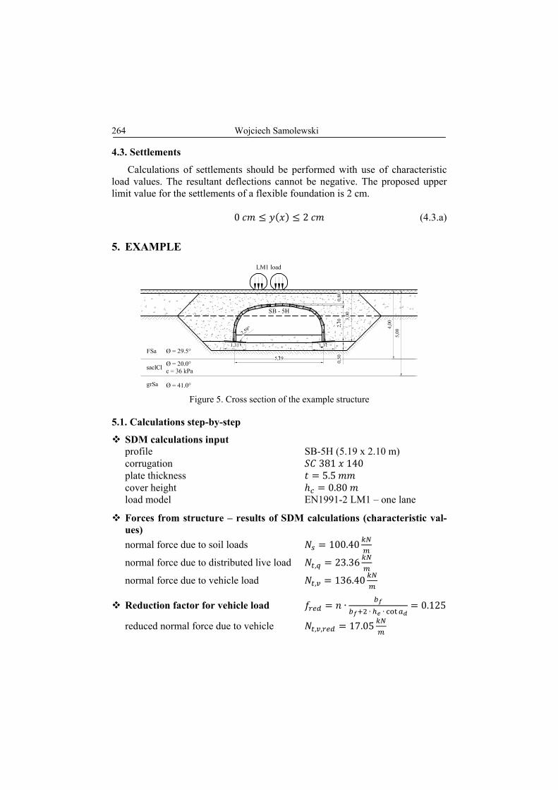
5. EXAMPLE

Figure 5. Cross section of the example structure

5.1. Calculations step-by-step

SDM calculations input profile SB-5H (5.19 x 2.10 m) corrugation 381 140 plate thickness 5.5 cover height 0.80 load model EN1991-2 LM1 – one lane

Forces from structure – results of SDM calculations (characteristic val-ues)

normal force due to soil loads 100.40

normal force due to distributed live load , 23.36

normal force due to vehicle load , 136.40

Reduction factor for vehicle load ∙∙ ∙

0.125

reduced normal force due to vehicle , , 17.05


Flexible foundation parameters length 1.305 corrugation 200 55 plate thickness 3

plastic modulus of section 62.30

yield strength of steel 355 modulus of elasticity 210

Gravel foundation material properties

weight 20.2

deformation modulus 60 angle of internal friction 35°

Foundation loads outside part (soil pressure + traffic load) , 93.96 central part 1961.95 inside part (soil pressure) , 10.91

Soil modulus calculation assumed pressure level under foundation 200 settlement calculation range 6.04 (acc. to 3.2.k) calculated settlement 5.5

equivalent soil modulus 36.2

Solution of the beam on Winkler foundation foundation stiffness parameter 0.419

Chart 1 – Design bending moment

position of max. bending moment point 0.653

maximum bending moment 21.47∙


Chart 2 – Foundation deflections

position of maximum deflection 0.624 maximum deflection 11.21 position of minimum deflection 1.305 maximum deflection 1.83

Subsoil bearing capacity , 320

Design conditions evaluation

cross section moment resistance 22.12∙

maximum stress under foundation , 307 , ,

settlements 11.21 20 1.83 0

5.2. Results evaluation

The results of the calculations presented in point 5.1. have been compared to analogous FEM results. The FEM analysis was performed in Plaxis 2D software. Staged erection of the backfill was included. The model is presented in the draw-ing below.

Figure 6. FEM analysis model

A

Perforand deflecof a beambelow.

Analytical met

rmed FEM actions that wm on Winkle

Chart 3 –

Chart 4 – D

thod for desig

analysis yieldwere very simer foundatio

– Design valu

Design values

Chart 5 –

gning flexible

ded values omilar to thoseon. The com

ues of pressure

of bending m

– Foundation d

foundations fo

of soil pressue showed by

mparison is p

es under the fo

moments in the

deflections

for soil-steel …

ures, bendingthe analytic

presented in

oundation

e foundation

… 267

g moments al solution the charts


6. SUMMARY

The paper presents and evaluates the use of standard foundation engineering solution of a beam on an elastic surface in the design of flexible foundations made of corrugated steel plates. It has been proven that the proposed analytical method produces results convergent with FEM analysis. The method can be easily implemented in any popular mathematic modeling software such as Mi-crosoft Excel and reduce labor consumption.

In the first part it is stated that the values of the forces acting on any founda-tion of soil-steel composite structure cannot be taken directly from the analytical calculations of the structure itself. The normal force should be reduced due to longitudinal load distribution. Also, it is stated that while the value of horizontal force is predictable in the central part of a structure cut to slope, it is not easy to calculate in the cut part.

The next part present formulation of the problem of a beam on Winkler foundation, soil modulus determination and design conditions which constitute optimization task boundaries. The above formulated tasks are illustrated with an example included in the last part of the report.

LITERATURE

1. Petterson L., Sundquist H., Design of soil steel composite bridges, TRITA-BKN. Report 112, 5th Edition 2014.

2. Wiłun Z., Zarys geotechniki, Wydawnictwo Komunikacji i Łączności, Warszawa 2013

3. PLAXIS 2D Tutorial Manual, available online [2017-01-16] https://www.plaxis.com/support/manuals/plaxis-2d-manuals/

4. PN-EN 1991-2 Eurocode 1: Actions on structures – Part 2: Traffic loads on bridges 5. PN-EN 1993-1 Eurocode 3: Design of steel structures – Part 1-1: General rules and

rules for buildings 6. PN-EN 1997-1 Eurocode 7: Geotechnical design – Part 1: General rules 7. PN-81/B-03020 Building soils. Foundation bases. Static calculations and design. 8. Belki a podłożu sprężystym, available online [2017-01-16]

http://limba.wil.pk.edu.pl/~jg/wyklady_wm/dzienne_1_stop/winkler/bnsp_teo.pdf

ERRATA

21. Wojciech Samolewski: Analytical method for designing flexible foundations for soil-steel composite structures

p. 259 Table 2. Functions (f) to calculate the coefficients of the variables in the system of linear equations ord. A B C D

0 𝑒−𝜉 sin 𝜉 𝑒−𝜉 cos 𝜉 𝑒𝜉 sin 𝜉 𝑒𝜉 cos 𝜉

I 𝑒−𝜉(−sin 𝜉 + cos𝜉) −𝑒−𝜉(sin 𝜉 + cos 𝜉) 𝑒𝜉(sin 𝜉 + cos 𝜉) 𝑒𝜉(−sin 𝜉 + cos 𝜉) II −2𝑒−𝜉 cos 𝜉 2𝑒−𝜉 sin 𝜉 2𝑒𝜉 cos𝜉 −2𝑒𝜉 sin 𝜉

III 2𝑒−𝜉(sin 𝜉 + cos𝜉) 2𝑒−𝜉(− sin 𝜉 + cos 𝜉) 2𝑒𝜉(− sin 𝜉 + cos 𝜉) −2𝑒𝜉(sin 𝜉 + cos 𝜉)

p. 259 Table 3. Matrix (F) of coefficients of the variables in the system of linear equations

equat. AL BL CL DL AC BC CC DC AR BR CR DR

(3.1.t) 𝑓𝐴,𝐼𝐼(𝜉𝑎) 𝑓𝐵,𝐼𝐼(𝜉𝑎) 𝑓𝐶,𝐼𝐼(𝜉𝑎) 𝑓𝐷,𝐼𝐼(𝜉𝑎) 0 0 0 0 0 0 0 0

(3.1.v) 𝑓𝐴,𝐼𝐼𝐼(𝜉𝑎) 𝑓𝐵,𝐼𝐼𝐼(𝜉𝑎) 𝑓𝐶,𝐼𝐼𝐼(𝜉𝑎) 𝑓𝐷,𝐼𝐼𝐼(𝜉𝑎) 0 0 0 0 0 0 0 0

(3.1.x) 𝑓𝐴,0(𝜉𝑏) 𝑓𝐵,0(𝜉𝑏) 𝑓𝐶,0(𝜉𝑏) 𝑓𝐷,0(𝜉𝑏) −𝑓𝐴,0(𝜉𝑏) −𝑓𝐵,0(𝜉𝑏) −𝑓𝐶,0(𝜉𝑏) −𝑓𝐷,0(𝜉𝑏) 0 0 0 0

(3.1.z) 𝑓𝐴,𝐼(𝜉𝑏) 𝑓𝐵,𝐼(𝜉𝑏) 𝑓𝐶,𝐼(𝜉𝑏) 𝑓𝐷,𝐼(𝜉𝑏) −𝑓𝐴,𝐼(𝜉𝑏) −𝑓𝐵,𝐼(𝜉𝑏) −𝑓𝐶,𝐼(𝜉𝑏) −𝑓𝐷,𝐼(𝜉𝑏) 0 0 0 0

(3.1.ab) 𝑓𝐴,𝐼𝐼(𝜉𝑏) 𝑓𝐵,𝐼𝐼(𝜉𝑏) 𝑓𝐶,𝐼𝐼(𝜉𝑏) 𝑓𝐷,𝐼𝐼(𝜉𝑏) −𝑓𝐴,𝐼𝐼(𝜉𝑏) −𝑓𝐵,𝐼𝐼(𝜉𝑏) −𝑓𝐶,𝐼𝐼(𝜉𝑏) −𝑓𝐷,𝐼𝐼(𝜉𝑏) 0 0 0 0

(3.1.ad) 𝑓𝐴,𝐼𝐼𝐼(𝜉𝑏) 𝑓𝐵,𝐼𝐼𝐼(𝜉𝑏) 𝑓𝐶,𝐼𝐼𝐼(𝜉𝑏) 𝑓𝐷,𝐼𝐼𝐼(𝜉𝑏) −𝑓𝐴,𝐼𝐼𝐼(𝜉𝑏) −𝑓𝐵,𝐼𝐼𝐼(𝜉𝑏) −𝑓𝐶,𝐼𝐼𝐼(𝜉𝑏) −𝑓𝐷,𝐼𝐼𝐼(𝜉𝑏) 0 0 0 0

(3.1.y) 0 0 0 0 −𝑓𝐴,0(𝜉𝑐) −𝑓𝐵,0(𝜉𝑐) −𝑓𝐶,0(𝜉𝑐) −𝑓𝐷,0(𝜉𝑐) 𝑓𝐴,0(𝜉𝑐) 𝑓𝐵,0(𝜉𝑐) 𝑓𝐶,0(𝜉𝑐) 𝑓𝐷,0(𝜉𝑐)

(3.1.aa) 0 0 0 0 −𝑓𝐴,𝐼(𝜉𝑐) −𝑓𝐵,𝐼(𝜉𝑐) −𝑓𝐶,𝐼(𝜉𝑐) −𝑓𝐷,𝐼(𝜉𝑐) 𝑓𝐴,𝐼(𝜉𝑐) 𝑓𝐵,𝐼(𝜉𝑐) 𝑓𝐶,𝐼(𝜉𝑐) 𝑓𝐷,𝐼(𝜉𝑐)

(3.1.ac) 0 0 0 0 −𝑓𝐴,𝐼𝐼(𝜉𝑐) −𝑓𝐵,𝐼𝐼(𝜉𝑐) −𝑓𝐶,𝐼𝐼(𝜉𝑐) −𝑓𝐷,𝐼𝐼(𝜉𝑐) 𝑓𝐴,𝐼𝐼(𝜉𝑐) 𝑓𝐵,𝐼𝐼(𝜉𝑐) 𝑓𝐶,𝐼𝐼(𝜉𝑐) 𝑓𝐷,𝐼𝐼(𝜉𝑐)

(3.1.ae) 0 0 0 0 −𝑓𝐴,𝐼𝐼𝐼(𝜉𝑐) −𝑓𝐵,𝐼𝐼𝐼(𝜉𝑐) −𝑓𝐶,𝐼𝐼𝐼(𝜉𝑐) −𝑓𝐷,𝐼𝐼𝐼(𝜉𝑐) 𝑓𝐴,𝐼𝐼𝐼(𝜉𝑐) 𝑓𝐵,𝐼𝐼𝐼(𝜉𝑐) 𝑓𝐶,𝐼𝐼𝐼(𝜉𝑐) 𝑓𝐷,𝐼𝐼𝐼(𝜉𝑐)

(3.1.u) 0 0 0 0 0 0 0 0 𝑓𝐴,𝐼𝐼(𝜉𝑑) 𝑓𝐵,𝐼𝐼(𝜉𝑑) 𝑓𝐶,𝐼𝐼(𝜉𝑑) 𝑓𝐷,𝐼𝐼(𝜉𝑑)

(3.1.w) 0 0 0 0 0 0 0 0 𝑓𝐴,𝐼𝐼𝐼(𝜉𝑑) 𝑓𝐵,𝐼𝐼𝐼(𝜉𝑑) 𝑓𝐶,𝐼𝐼𝐼(𝜉𝑑) 𝑓𝐷,𝐼𝐼𝐼(𝜉𝑑)

p. 260 line 7 from the top


Values of foundation modulus (Cf) for subsoils consisting of one soil material can be found in literature. The values

vary from 𝟓 𝑘𝑁𝑚3

for very weak soils (such as silts or clays) up to 40 𝑘𝑁𝑚3

for stronger soils (such as gravels or compacted

sands).

ERRATA

21. Wojciech Samolewski: Analytical method for designing flexible foundations for soil-steel composite structures

p. 259 Table 2. Functions (f) to calculate the coefficients of the variables in the system of linear equations ord. A B C D

0 𝑒−𝜉 sin 𝜉 𝑒−𝜉 cos 𝜉 𝑒𝜉 sin 𝜉 𝑒𝜉 cos 𝜉

I 𝑒−𝜉(−sin 𝜉 + cos𝜉) −𝑒−𝜉(sin 𝜉 + cos 𝜉) 𝑒𝜉(sin 𝜉 + cos 𝜉) 𝑒𝜉(−sin 𝜉 + cos 𝜉) II −2𝑒−𝜉 cos 𝜉 2𝑒−𝜉 sin 𝜉 2𝑒𝜉 cos𝜉 −2𝑒𝜉 sin 𝜉

III 2𝑒−𝜉(sin 𝜉 + cos𝜉) 2𝑒−𝜉(− sin 𝜉 + cos 𝜉) 2𝑒𝜉(− sin 𝜉 + cos 𝜉) −2𝑒𝜉(sin 𝜉 + cos 𝜉)

p. 259 Table 3. Matrix (F) of coefficients of the variables in the system of linear equations

equat. AL BL CL DL AC BC CC DC AR BR CR DR

(3.1.t) 𝑓𝐴,𝐼𝐼(𝜉𝑎) 𝑓𝐵,𝐼𝐼(𝜉𝑎) 𝑓𝐶,𝐼𝐼(𝜉𝑎) 𝑓𝐷,𝐼𝐼(𝜉𝑎) 0 0 0 0 0 0 0 0

(3.1.v) 𝑓𝐴,𝐼𝐼𝐼(𝜉𝑎) 𝑓𝐵,𝐼𝐼𝐼(𝜉𝑎) 𝑓𝐶,𝐼𝐼𝐼(𝜉𝑎) 𝑓𝐷,𝐼𝐼𝐼(𝜉𝑎) 0 0 0 0 0 0 0 0

(3.1.x) 𝑓𝐴,0(𝜉𝑏) 𝑓𝐵,0(𝜉𝑏) 𝑓𝐶,0(𝜉𝑏) 𝑓𝐷,0(𝜉𝑏) −𝑓𝐴,0(𝜉𝑏) −𝑓𝐵,0(𝜉𝑏) −𝑓𝐶,0(𝜉𝑏) −𝑓𝐷,0(𝜉𝑏) 0 0 0 0

(3.1.z) 𝑓𝐴,𝐼(𝜉𝑏) 𝑓𝐵,𝐼(𝜉𝑏) 𝑓𝐶,𝐼(𝜉𝑏) 𝑓𝐷,𝐼(𝜉𝑏) −𝑓𝐴,𝐼(𝜉𝑏) −𝑓𝐵,𝐼(𝜉𝑏) −𝑓𝐶,𝐼(𝜉𝑏) −𝑓𝐷,𝐼(𝜉𝑏) 0 0 0 0

(3.1.ab) 𝑓𝐴,𝐼𝐼(𝜉𝑏) 𝑓𝐵,𝐼𝐼(𝜉𝑏) 𝑓𝐶,𝐼𝐼(𝜉𝑏) 𝑓𝐷,𝐼𝐼(𝜉𝑏) −𝑓𝐴,𝐼𝐼(𝜉𝑏) −𝑓𝐵,𝐼𝐼(𝜉𝑏) −𝑓𝐶,𝐼𝐼(𝜉𝑏) −𝑓𝐷,𝐼𝐼(𝜉𝑏) 0 0 0 0

(3.1.ad) 𝑓𝐴,𝐼𝐼𝐼(𝜉𝑏) 𝑓𝐵,𝐼𝐼𝐼(𝜉𝑏) 𝑓𝐶,𝐼𝐼𝐼(𝜉𝑏) 𝑓𝐷,𝐼𝐼𝐼(𝜉𝑏) −𝑓𝐴,𝐼𝐼𝐼(𝜉𝑏) −𝑓𝐵,𝐼𝐼𝐼(𝜉𝑏) −𝑓𝐶,𝐼𝐼𝐼(𝜉𝑏) −𝑓𝐷,𝐼𝐼𝐼(𝜉𝑏) 0 0 0 0

(3.1.y) 0 0 0 0 −𝑓𝐴,0(𝜉𝑐) −𝑓𝐵,0(𝜉𝑐) −𝑓𝐶,0(𝜉𝑐) −𝑓𝐷,0(𝜉𝑐) 𝑓𝐴,0(𝜉𝑐) 𝑓𝐵,0(𝜉𝑐) 𝑓𝐶,0(𝜉𝑐) 𝑓𝐷,0(𝜉𝑐)

(3.1.aa) 0 0 0 0 −𝑓𝐴,𝐼(𝜉𝑐) −𝑓𝐵,𝐼(𝜉𝑐) −𝑓𝐶,𝐼(𝜉𝑐) −𝑓𝐷,𝐼(𝜉𝑐) 𝑓𝐴,𝐼(𝜉𝑐) 𝑓𝐵,𝐼(𝜉𝑐) 𝑓𝐶,𝐼(𝜉𝑐) 𝑓𝐷,𝐼(𝜉𝑐)

(3.1.ac) 0 0 0 0 −𝑓𝐴,𝐼𝐼(𝜉𝑐) −𝑓𝐵,𝐼𝐼(𝜉𝑐) −𝑓𝐶,𝐼𝐼(𝜉𝑐) −𝑓𝐷,𝐼𝐼(𝜉𝑐) 𝑓𝐴,𝐼𝐼(𝜉𝑐) 𝑓𝐵,𝐼𝐼(𝜉𝑐) 𝑓𝐶,𝐼𝐼(𝜉𝑐) 𝑓𝐷,𝐼𝐼(𝜉𝑐)

(3.1.ae) 0 0 0 0 −𝑓𝐴,𝐼𝐼𝐼(𝜉𝑐) −𝑓𝐵,𝐼𝐼𝐼(𝜉𝑐) −𝑓𝐶,𝐼𝐼𝐼(𝜉𝑐) −𝑓𝐷,𝐼𝐼𝐼(𝜉𝑐) 𝑓𝐴,𝐼𝐼𝐼(𝜉𝑐) 𝑓𝐵,𝐼𝐼𝐼(𝜉𝑐) 𝑓𝐶,𝐼𝐼𝐼(𝜉𝑐) 𝑓𝐷,𝐼𝐼𝐼(𝜉𝑐)

(3.1.u) 0 0 0 0 0 0 0 0 𝑓𝐴,𝐼𝐼(𝜉𝑑) 𝑓𝐵,𝐼𝐼(𝜉𝑑) 𝑓𝐶,𝐼𝐼(𝜉𝑑) 𝑓𝐷,𝐼𝐼(𝜉𝑑)

(3.1.w) 0 0 0 0 0 0 0 0 𝑓𝐴,𝐼𝐼𝐼(𝜉𝑑) 𝑓𝐵,𝐼𝐼𝐼(𝜉𝑑) 𝑓𝐶,𝐼𝐼𝐼(𝜉𝑑) 𝑓𝐷,𝐼𝐼𝐼(𝜉𝑑)

p. 260 line 7 from the top


Values of foundation modulus (Cf) for subsoils consisting of one soil material can be found in literature. The values

vary from 𝟓 𝑘𝑁𝑚3

for very weak soils (such as silts or clays) up to 40 𝑘𝑁𝑚3

for stronger soils (such as gravels or compacted

sands).

analytical method for designing flexible foundations · pdf fileanalytical method for...

Documents