1

Analytic Modeling Approach to Business Decision Making: 1. Type of general business models

o Mental model o Visual model o Prototype or physical or scale model o Mathematical models: forecasting, regression, decision, queueing, simulation, LP/ILP models

Profit = Revenue – Expenses Profit=�(Revenue, Expenses) � = �(��, ��) � = �(��, ��, ⋯ , ��) where �� is the variable i in the model for i = 1, 2, …, k

2. Categories of Mathematical Models Figure 1.3 (Ragsdale, pp.6)

Model Characteristics Category Form of �(. ) Values of

Independent variables Management Science Techniques

Prescriptive Models

Known, well-defined

Known or under decision maker’s control

LP, Network, ILP, CPM, Goal Programming, EOQ, Nonlinear Programming

Predictive Models

Unknown, ill-defined

Known or under decision maker’s control

Regression analysis, Time series analysis, Discriminant analysis

Descriptive Models

Known, well defined

Unknown or uncertain Queueing, Simulation, PERT, Inventory models

3. The process to use analytic modeling in Business Decision Making

4. Anchoring and Framing Effects

o Anchor effect: under adjust position relative to Anchor � 1 × 2 × 3 × 4 × 5 × 6 × 7 × 8 versus 8 × 7 × 6 × 5 × 4 × 3 × 2 × 1

o Framing effect: � Sure Win Prospective: Given $1,000 and A1 to receive another $500 or B1 to flip a coin to

get $1,000 more if it is head or to get $0 if it is tail. � Sure Loss Prospective: Given $2,000 and A2 to give back $500 or B2 to flip a coin to give

back $0 if it is head or to give back $1,000 if it is tail. 5. Good Decisions versus Good Outcomes

Good Outcome Bad Outcome Good Decision 65 5 70 Bad Decision 5 25 30 70 30 100

P(Good Outcome | Good Decision)=65/70=92.86% P(Bad outcome | Good Decision)=5/70=7.14% P(Good Outcome | Bad Decision)=5/30=16.67% P(Bad Outcome | Bad Decisioin)=25/30=83.33%

6. Business benefits from analytic modeling o Simplicity o More economically sound o Quick result o Examine many things that otherwise could not be possibly be studied o Gain insights into business decision making

2

Forecasting (http://en.wikipedia.org/wiki/Forecasting) Adam, the manager of customer service department, would like to forecast the number of calls to customer service

in order for him to schedule his staff members. The historical data are given in the following table.

The model to be used is: ����� = �(�� , ����, ⋯ , ��) or the forecast for the period t+1 is the function of the historical

data.

How to develop the forecasts? We will use several methods, including: Simple Moving Average (3), Weighted

Moving Average (3), and Exponential Smoothing. Regression will be discussed later.

How shall the forecasting accuracy of each method be evaluated? We will use Mean Absolute Error (MAE), Mean

Absolute Percentage Error (MAPE), and Mean Squared Error (MSE). The smaller the values of MAE, MAPE and MSE,

the better, the forecast.

3

The answers to the class exercises are given here.

4

Use Excel@ in developing forecasting models:

1. Use Excel@ formulas: =SUMPRODUCT(), =SUMXMY2(), etc.

2. Use or not use the absolute cell address ($I$111) in Excel@ formulas

3. Excel@ may have more than one way (or formula) to carry out a task (compute WMA or EXP), which one

should be used?

4. Use Excel@ Solver or PremSolver to Minimize MSE in order to find the optimal weights for WMA or the

optimal smoothing constant for Exponential Smoothing.

Please try out each of the following Excel@ formulas after the class.

The equations used to develop the answers in Excel@ are given in the following table with Excel@ Formula/Show

Formulas option.

5

6

Topics to be covered: 1. Forecasting, qualitative and quantitative forecasting methods

a. Qualitative forecasting methods: Executive Judgment, Historical analogy, Delphi method, Grass roots, Market research, and Panel consensus.

b. Quantitative forecasting methods:

i. Classical Time Series Model � = � • � • � • � where T, C, S and I refer to the Trend, Cyclical, Seasonal and Irregular component of a time series. Seasonality refers to, any seasonal variations, such as, hourly, daily, weekly, monthly or quarterly effect, that is normally within a year. The Cyclical effect is normally longer than a year, mostly caused by economical cycles and is harder to study.

ii. Simple Moving Average (SMA) & Naïve Forecast iii. Weighted Moving Average (WMA) iv. Centered Moving Average and Seasonal Factor v. Exponential Smoothing vi. Simple Linear Regression (SLR) vii. Associative methods:

� Simple Linear regression � Multiple Linear regression

ii. Combining Forecast

2. Assumptions for quantitative forecasting methods

3. Forecasting Accuracy and Selection of Forecasting Methods Forecasting Time Line:

Yt = the actual observation or value of the variable to be forecast for the most recent time period t Prior observations are noted by subtracting 1 from time period t. ����� = the forecasted value for the next period. Following periods are designated by adding 1 to time period t+1.

Forecasting

1. Assumes causal system: past ==> future. The future is going to resemble that of the past. 2. Forecasts rarely perfect because of randomness, What that means “Forecast is always wrong, with 50%

over forecast and 50% under forecast” ? 3. Forecasts more accurate for groups (product families, i.e. passenger cars) vs. individuals (i.e. Toyota Camry) 4. Forecast accuracy decreases as time horizon increases

Time Series Forecasts

1. Trend - long-term movement in data 2. Seasonality - short-term regular variations in data 3. Irregular variations - caused by unusual circumstances 4. Random variations - caused by chance

7

Seasonal Variations • Regular repeating movements in time series values that can be tied to recurring events • Annual variations: weather, summer/winter sports equipment • Vacations/holidays: airline travel, greeting cards, resort • Daily, Weekly, Monthly: rush traffic hours, theaters and restaurants, banks, mail volume, sales of

toys, beer, automobiles, turkeys, highway usage, hotel registrations, gardening, public transportations, electric power plants

Multiplicative Seasonal Model

• Forecast = Trend x SI x Random Components • SI = Seasonal Index or Relatives or Percentages • SI = 1.20 for May, thus Sales in May are 20% above the monthly average • SI = 0.90 for July, thus Sales in July are only 90% of the monthly average

Forecasting Procedures

• Determine the purpose and time: level of details, resources (manpower, computing times, etc), level of accuracy

• Establish a time horizon • Select a forecasting technique • Collect and analyze the data, and prepare the forecast, identify any assumptions • Monitor the forecast

8

Example 1, Customer Calls

Mean Error (ME):

! = 1" # (�� − ���)%

�&�

Mean Absolute Error (MAE):

'! = 1" # |�� − ���|%

�&�

Mean Absolute Percentage Error (MAPE):

')! = 1" # *�� − ����� *%

�&�

Sum of Squared Error (SSE):

��! = # (�� − ���)�%�&�

Mean Squared Error (MSE):

�! = 1" # (�� − ���)�%

�&� = ��!"

Root Mean Squared Error (RMSE): RMSE = √ �! To see Formulas in Excel, click Formulas/Show Formulas MSE

0

5

10

15

20

25

30

35

40

1 2 3 4 5 6

Yt

Yt

=SUMXMY2($B$8:$B$10,C8:C10)/COUNT(C8:C10)

9

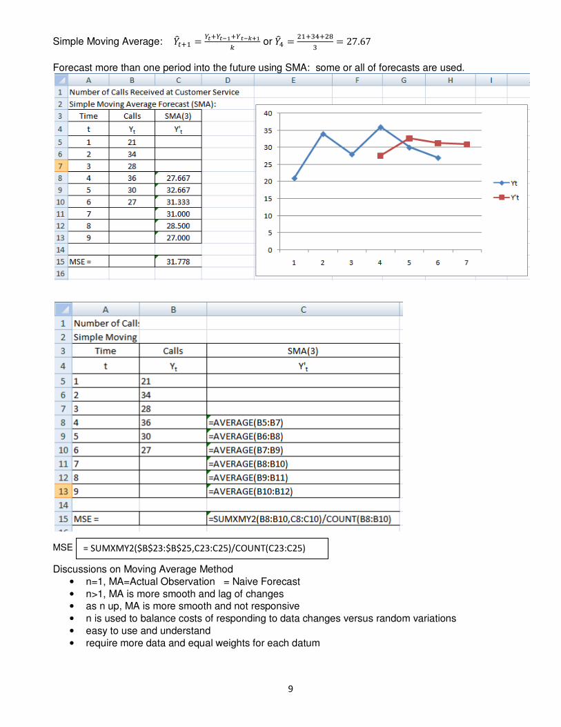
Simple Moving Average: ����� = ,-�,-./�,-.01/� or ��2 = ���32��4

3 = 27.67

Forecast more than one period into the future using SMA: some or all of forecasts are used.

MSE

Discussions on Moving Average Method • n=1, MA=Actual Observation = Naive Forecast • n>1, MA is more smooth and lag of changes • as n up, MA is more smooth and not responsive • n is used to balance costs of responding to data changes versus random variations • easy to use and understand • require more data and equal weights for each datum

= SUMXMY2($B$23:$B$25,C23:C25)/COUNT(C23:C25)

10

Let us look at the details of SMA forecast again: ��2 = ���32��43 = 27.67 = �

3 (21) + �3 (34) + �

3 (28) = 27.67

In another word, an equal weight of 1/3 is signed to each of the past observations to get the forecast. It is often argued that the importance of each of the past observations differs in forecasting future value, thus the use of Weighted Moving Average Forecasting (WMA). Weighted Moving Average Forecasting (WMA): ����� = 61 × �� + 62 × ���� + ⋯ + 67 × ������ where k is the number of past observations used in developing the forecast. For a 3 period weighted moving average, k=3.

��2 = 0.5 × 28 + 0.3 × 34 + 0.2 × 21 = 28.40

=SUMPRODUCT($K$37:$K$39,B37:B39)

=$K$39*B39+$K$38*B38+$K$37*B37

11

Using Excel@ Solver to optimize weights in WMA forecasting: Objective function: Min MSE {=SUMXMY2(B25:B27,C25:C27)/COUNT(B25:B27)} Constraints: s.t. W1, W2, W3 ≥ 0 W1, W2, W3 ≤ 1 W1 + W2 + W3 = 1 Adjust Cells: F22:F24

In order to use Excel Solver to minimize MSE to get the optimal weights, click Data/Solver

0

10

20

30

40

1 2 3 4 5 6 7

Yt

Y't

12

Weighted Moving Average � MA is a special case of WMA with all of the weights are equal. � Choice of weights Ws with Excel Data/Solver is a non linear optimization problem due to MSE � Choice of n: may try n = 2, 3, or 4 and use Data/Solver to find the n value with minimum MSE

Forecast more than one period into the future using WMA: some or all of forecasts may be used.

Exponential Smoothing Forecast: ����� = ��� + 9:�� − ���; = 9(��) + (1 − 9)��� = 9(��) + 9(1 − 9)���� + ⋯

Using Excel@ Solver to optimize α value in Exponential smoothing forecast: Objective function: Min MSE {=SUMXMY2(B42:B44,C42:C44)/COUNT(B42:B44)} Constrarints: s.t. α ≥ 0 and α ≤ 1 Adjust Cells: F39

=C86+$K$84*(B86-C86)

13

0

5

10

15

20

25

30

35

40

1 2 3 4 5 6 7

Yt

Y't

14

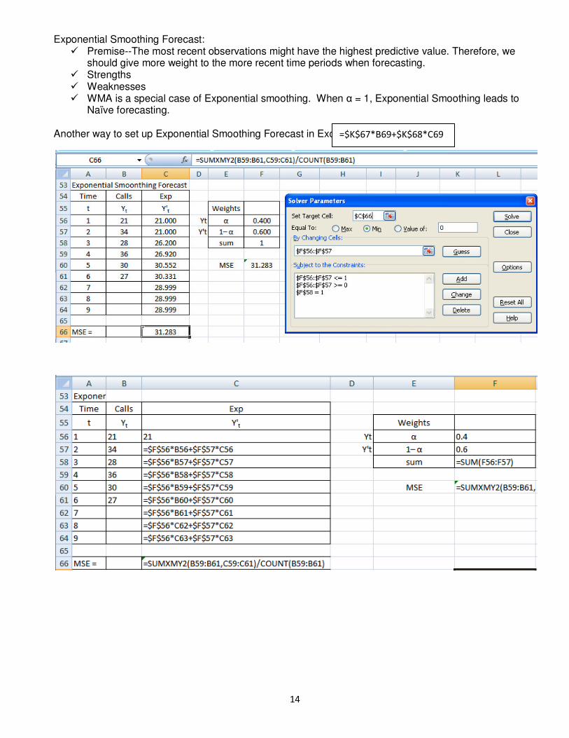
Exponential Smoothing Forecast: � Premise--The most recent observations might have the highest predictive value. Therefore, we

should give more weight to the more recent time periods when forecasting. � Strengths � Weaknesses � WMA is a special case of Exponential smoothing. When α = 1, Exponential Smoothing leads to

Naïve forecasting. Another way to set up Exponential Smoothing Forecast in Excel:

=$K$67*B69+$K$68*C69

15

16

Picking a Smoothing Constant α with Excel Data/Solver Discussions on Exponential Smoothing

� α - positively related to responsiveness � α -(0.05-0.50) and trial and error � easy to calculate and need minimum of data � widely used � α up - more weight on recent obs � not useful if trend exists

How to develop a forecast if the data has Trend, Seasonality and Random components? Here is the SUV Sales data from Ragsdale 5th Edition.

Year Quarter Time Units Sold

2003 1 1 23

2 2 25

3 3 36

4 4 31

2004 1 5 26

2 6 28

3 7 48

4 8 36

2005 1 9 31

2 10 42

3 11 53

4 12 43

2006 1 13 --

2 14 --

3 15 --

4 16 --

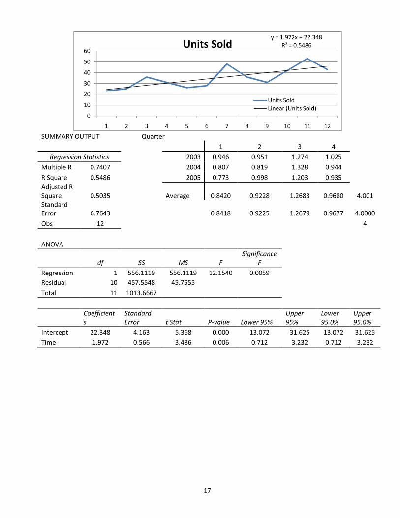
Given the data for Number of SUV sold, develop forecst for 2006 1. Use Excel@ Insert/Line Chart to draw the data. It appears the data has trend and quarterly

seasonality 2. Use Excel Data/Data Analysis/Regression to find values for the b0 and b1, the regression line, and

R Square value. 3. Use Hypothesis Test to test β0 and β1 to be sure they are not zeros, i.e. p-value for each is very

small < 0.05 4. Use the model Y = T. C. S. I = Trend.Cycle.Season.Irregular 5. Use Excel =Intercept() and =Slope () as below to get the B0 and B1 for the Regression Line Trend,

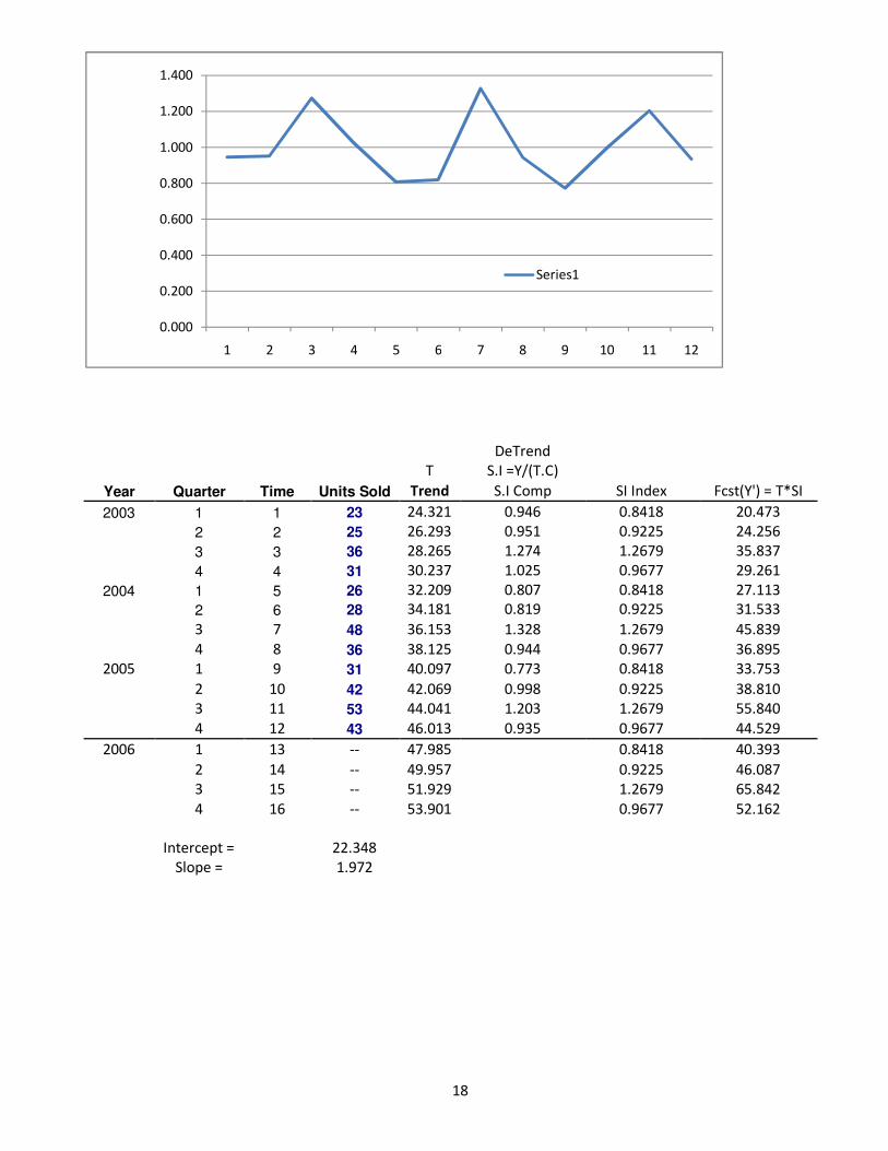
i.e. 1.972 x + 22.34 = Y 6. S.I Relative = Units Sold (Y) / Trend, i.e. 23/24.321 = 0.946 7. Create a table with S.I Relatives in the same quarter lined up together as in the Table 8. Use =Average () to get the average of the S.I Relatives for each quarter and sum up the four S.I

Relatives to 4.001, i.e. =average() = 0.8420 for the first quarter 9. Use each quarter S.I Relative divides 4.001 and times 4.000 as adjustment, i.e.

0.8420/4.001*4.000=0.8418 as SI Index 10. Create a column SI Index, and use the same SI Index for the same quarter of each year, i.e.

0.8418 for first quarter of each year 11. Use Trend * SI Index to get the Seasonally Adjusted Fcst (Y'), i.e. 24.321 * 0.8418 = 20.473 for

2003.1 Quarter 12. Use Excel to plot Fcst (Y') and Units Sold to show how well the forecast is to be

17

SUMMARY OUTPUT

Quarter

1 2 3 4

Regression Statistics

2003 0.946 0.951 1.274 1.025

Multiple R 0.7407

2004 0.807 0.819 1.328 0.944

R Square 0.5486

2005 0.773 0.998 1.203 0.935

Adjusted R

Square 0.5035

Average 0.8420 0.9228 1.2683 0.9680 4.001

Standard

Error 6.7643

0.8418 0.9225 1.2679 0.9677 4.0000

Obs 12

4

ANOVA

df SS MS F

Significance

F

Regression 1 556.1119 556.1119 12.1540 0.0059

Residual 10 457.5548 45.7555

Total 11 1013.6667

Coefficient

s

Standard

Error t Stat P-value Lower 95%

Upper

95%

Lower

95.0%

Upper

95.0%

Intercept 22.348 4.163 5.368 0.000 13.072 31.625 13.072 31.625

Time 1.972 0.566 3.486 0.006 0.712 3.232 0.712 3.232

y = 1.972x + 22.348

R² = 0.5486

0

10

20

30

40

50

60

1 2 3 4 5 6 7 8 9 10 11 12

Units Sold

Units Sold

Linear (Units Sold)

18

DeTrend

T S.I =Y/(T.C)

Year Quarter Time Units Sold Trend S.I Comp SI Index Fcst(Y') = T*SI

2003 1 1 23 24.321 0.946 0.8418 20.473

2 2 25 26.293 0.951 0.9225 24.256

3 3 36 28.265 1.274 1.2679 35.837

4 4 31 30.237 1.025 0.9677 29.261

2004 1 5 26 32.209 0.807 0.8418 27.113

2 6 28 34.181 0.819 0.9225 31.533

3 7 48 36.153 1.328 1.2679 45.839

4 8 36 38.125 0.944 0.9677 36.895

2005 1 9 31 40.097 0.773 0.8418 33.753

2 10 42 42.069 0.998 0.9225 38.810

3 11 53 44.041 1.203 1.2679 55.840

4 12 43 46.013 0.935 0.9677 44.529

2006 1 13 -- 47.985

0.8418 40.393

2 14 -- 49.957

0.9225 46.087

3 15 -- 51.929

1.2679 65.842

4 16 -- 53.901

0.9677 52.162

Intercept =

22.348

Slope =

1.972

0.000

0.200

0.400

0.600

0.800

1.000

1.200

1.400

1 2 3 4 5 6 7 8 9 10 11 12

Series1

19

Combining Forecast with varying weights Summary of Forecast:

• Limitations of forecasting capabilities o It is more of art than science o Combining forecast generates improved performance

• None of the criterion to evaluate forecasting accuracy performs better than others – you make your choice based upon your personal preference and industry practice

• Quantitative forecasting methods show to outperform qualitative methods over time. • Be aware of the possible mistakes in using Excel and the potential damage from the mistakes.

0.000

10.000

20.000

30.000

40.000

50.000

60.000

70.000

1 2 3 4 5 6 7 8 9 10 11 12 13 14 15 16

Fcst(Y') = T*SI

Units Sold