analysis - university of cretefourier.math.uoc.gr/~papadim/calculus_on_manifolds/munkres.pdf ·...
TRANSCRIPT


Analysis on Manifolds
James R. Munkres Massachusetts Institute of Technology
Cambridge, Massachusetts
ADDISON-WESLEY PUBLISHING COMPANY The Advanced Book Program
Redwood City, California • Menlo Park, California • Reading, Massachusetts New York • Don Mills, Ontario • Wokingham, United Kingdom • Amsterdam
Bonn • Sydney •Singapore • Tokyo • Madrid • San Juan

Publisher: Allan M. Wylde Production Manager: Jan V. Benes Marketing Manager: Laura Likely Electronic Composition: Peter Vacek Cover Design: Iva Frank
Library of Congress Cataloging-in-Publication Data
Munkres, James R., 1930-Analysis on manifolds/James R. Munkres.
p. em. Includes bibliographical references. 1. Mathematical analysis. 2. Manifolds (Mathematics) QA300.M75 1990 5 16.3'6'2Q-dc20 ISBN 0-201-51035-9
91-39786 CIP
This book was prepared using the TEX typesetting language.
Copyright @1991 by Addison-Wesley Publishing Company, The Advanced Book Program, 350 Bridge Parkway, Suite 209, Redwood City, CA 94065
All rights reserved. No part of this publication may be reproduced, stored in a retrieval system, or transmitted, in any form, or by any means, electronic, mechanical, photocopying, recording or otherwise, without the prior written permission of the publisher. Printed in the United States of America. Published simultaneously in Canada.
ABCDEFGHIJ-MA-943210

Preface
This book is intended as a text for a course in analysis, at the senior or first-year graduate level.
A year-long course in real analysis is an essential part of the preparation of any potential mathematician. For the first half of such a course , there is substantial agreement as to what the syllabus should be. Standard topics include: sequence and series , the topology of metric spaces, and the derivative and the Riemannian integral for functions of a single variable. There are a number of excellent texts for such a course, including books by Apostol [A] , Rudin [Ru] , Goldberg [Go] , and Royden [Ro] , among others.
There is no such universal agreement as to what the syllabus of the second half of such a course should be . Part of the problem is that there are simply too many topics that belong in such a course for one to be able to treat them all within the confines of a single semester, at more than a superficial level.
At M.I.T., we have dealt with the problem by offering two independent second-term courses in analysis. One of these deals with the derivative and the Riemannian integral for functions of several variables, followed by a treatment of differential forms and a proof of Stokes' theorem for manifolds in euclidean space. The present book has resulted from my years of teaching this course, The other deals with the Lebesque integral in euclidean space and its applications to Fourier analysis.
Prequisites
As indicated, we assume the reader has completed a one-term course in analysis that included a study of metric spaces and of functions of a single variable. We also assume the reader has some background in linear algebra, including vector spaces and linear transformations, matrix algebra, and determinants.
The first chapter of the book is devoted to reviewing the basic results from linear algebra and analysis that we shall need. Results that are truly basic are
v

• VI Preface
stated without proof, but proofs are provided for those that are sometimes omitted in a first course . The student may determine from a perusal of this chapter whether his or her background is sufficient for the rest of the book.
How much time the instructor will wish to spend on this chapter will depend on the experience and preparation of the students. I usually assign Sections 1 and 3 as reading material, and discuss the remainder in class.
How the book is organized
The main part of the book falls into two parts. The first, consisting of Chapter 2 through 4, covers material that is fairly standard: derivatives, the inverse function theorem, the Riemann integral , and the change of variables theorem for multiple integrals. The second part of the book is a bit more sophisticated. It introduces manifolds and differential forms in Rn, providing the framework for proofs of the n-dimensional version of Stokes' theorem and of the Poincare lemma.
A final chapter is devoted to a discussion of abstract manifolds; it is intended as a transition to more advanced texts on the subject.
The dependence among the chapters of the book is expressed in the following diagram:
Chapter 1
Chapter 2
Chapter 3
Chapter 4
Chapter 5
Chapter 7
Chapter 9
The Algebra and Topology of Rn
� Different iation
� Integration
� . Change of Vanables
MLifolds
Chapter 6 Differential Forms
I Stokes' Theorem
Chapter 8 Closed Forms and Exact Forms
Epilogue-Life Outside Rn

Preface
Certain sections of the books are marked with an asterisk; these sections may be omitted without loss of continuity. Similarly, certain theorems that may be omitted are marked with asterisks. When I use the book in our undergraduate analysis sequence , I usually omit Chapter 8, and assign Chapter 9 as reading. With graduate students, it should be possible to cover the entire book.
At the end of each section is a set of exercises. Some are computational in nature; students find it illuminating to know that one can compute the volume of a five-dimensional ball, even if the practical applications are limited! Other exercises are theoretical in nature, requiring that the student analyze carefully the theorems and proofs of the preceding section. The more difficult exercises are marked with asterisks, but none is unreasonably hard.
Acknowledgements
Two pioneering works in this subject demonstrated that such topics as manifolds and differential forms could be discussed with undergraduates . One is the set of notes used at Princeton c. 1960, written by Nickerson, Spencer, and Steenrod [N-S-S] . The second is the book by Spivak [S] . Our indebtedness to these sources is obvious. A more recent book on these topics is the one by Guillemin and Pollack [ G-P] . A number of texts treat this material at a more advanced level . They include books by Boothby [B] , Abraham, Mardsen, and Raitu [A-M-R], Berger and Gostiaux [B-G] , and Fleming [F] . Any of them would be suitable reading for the student who wishes to pursue these topics further.
I am indebted to Sigurdur Helgason and Andrew Browder for helpful comments. To Ms. Viola Wiley go my thanks for typing the original set of lecture notes on which the book is based. Finally, thanks is due to my students at M.I.T., who endured my struggles with this material , as I tried to learn how to make it understandable (and palatable) to them!
J .R.M.
•• VII


Contents
PREFACE v
CHAPTER 1 The Algebra and Topology of Rn 1
§ 1 . Review of Linear Algebra 1
§2 . Matrix Inversion and Determinants 1 1
§3. Review of Topology in Rn 25
§4. Compact Subspaces and Connected Subspaces of Rn 32
CHAPTER 2 Differentiation 41
§5. Derivative 4 1
§6. Continuously Differentiable Functions 49
§7 . The Chain Rule 56
§8 . The Inverse Function Theorem 63 *§9. The Implicit Function Theorem 71
• IX

X Contents
CHAPTER 3 Int egration
§ 10. The Integral over a Rectangle 81
§ 1 1 . Existence of the Integral 91
§ 1 2. Evaluation of the Integral 98
§13 . The Integral over a Bounded Set
§ 14. Rectifiable Sets 1 12
§ 15. Improper Integrals 121
CHAPTER 4 Chang es of Variabl es
§ 16. Partitions of Unity 136
104
§ 17. The Change of Variables Theorem 144
§ 18. Diffeomorphisms in Rn 152
§ 19 . Proof of the Change of Variables Theorem 160
§20. Application of Change of Variables 169
81
135
CHAPTER 5 Manifo lds 179
§21 . The Volumne of a Parallelopiped 178
§22. The Volume of a Parametrized-Manifold 186
§23. Manifolds in Rn 194
§24. The Boundary of a Manifold 20 1
§25. Integrating a Scalar Function over a Manifold 207
CHAPTER 6 Differ ential Forms
§26. Multilinear Algebra 220
§27. Alternating Tensors 226
§28. The Wedge Product 236
§29. Tangent Vectors and Differential Forms 244
§30. The Differential Operator 252 *§31. Application to Vector and Scalar Fields 262
§32. The Action of a Differentiable Map 267
219

• Contents XI
CHAPTER 7 Stok es' Th eor em 275
§33. Integrating Forms over Parametrized-Manifold 275 §34. Orientable Manifolds 281
§35. Integrating Forms over Oriented Manifolds 293 *§36.
§37. *§38.
CHAPTER 8
A Geometric Interpretation of Forms and Integrals
The Generalized Stokes' Theorem 301 Applications to Vector Analysis 310
Clos ed Forms and Exact Forms
§39. The Poincare Lemma 324
297
323
§40. The deRham Groups of Punctured Euclidean Space 334
CHAPTER 9 Epilogu e-Life Outsid e R" 345
§41 . Differentiable Manifolds and Riemannian Manifolds 345
BIBL IOGRAPHY 259


Analysis on Manifolds


The Algebra and Topology of Rn
§1. REVIEW OF LI NEAR ALGEBRA
Vector spaces
Suppose one is given a set V of objects, called v ectors . And suppose there is given an operation called v ector addition, such that the sum of the vectors x and y is a vector denoted x + y. Finally, suppose there is given an operation called scalar multiplication, such that the product of the scalar (i .e. , real number) e and the vector x is a vector denoted ex.
The set V, together with these two operations, is called a v ector spac e (or lin ear spac e) if the following properties hold for all vectors x, y, z and all scalars e, d:
(1) X+ y = y +X. (2) x + (y + z) = (x + y) + z. (3) There is a unique vector 0 such that x + 0 = x for all x. (4) x + (-l)x = 0.
(5) lx = x. (6) e(dx) = (ed)x. (7) ( e + d)x = ex + dx. (8) e(x+y) = ex+ey.
1

2 The Algebra and Topology of Rn Chapter 1
One example of a vector space is the set Rn of all n-tuples of real numbers, with component-wise addition and multiplication by scalars. That is, if x = (x1, . . . , Xn ) and y = (Yb . . . , Yn ), then
X+ y = (x 1 + Yb . . . , Xn + Yn), ex = (cxb . . . , cxn)·
The vector space properties are easy to check. If V is a vector space, then a subset W of V is called a lin ear subspac e
(or simply, a subspac e) of V if for every pair x,y of elements ofW and every scalar c, the vectors x + y and ex belong to W. In this case, W itself satisfies properties (1)-(8) if we use the operations that W inherits from V, so that W is a vector space in its own right.
In the first part of this book , Rn and its subspaces are the only vector spaces with which we shall be concerned. In later chapters we shall deal with more general vector spaces.
Let V be a vector space. A set a1 , . . . , am of vectors in V is said to span V if to each x in V, there corresponds at least one m-tuple of scalars ell ... , Cm such that
x = c1a1+···+Cmam. In this case, we say that x can be written as a lin ear combination of the vectors a1, . .. , am.
The set a1, . .. , am of vectors is said to be ind ep end ent if to each x in V there corresponds at most one m-tuple of scalars ell . . . , Cm such that
Equivalently, { a1, . . . , am} is independent if to the zero vector 0 there corresponds only one m-tuple of scalars d1, . . . , dm such that
0 = d1a1 + · · · + dmam,
namely the scalars d1 = d2 = · · · = dm = 0. If the set of vectors a1, .. . , am both spans V and is independent , it is
said to be a basis for V. One has the following result:
Th eor em 1.1. Suppose V has a basis consisting of m vectors. Then any set of vectors that spans V has at least m vectors, and any set of vectors of V that is independent has at most m vectors. In particular, any basis for V has exactly m vectors. D
If V has a basis consisting of m vectors , we say that m is the dim ension of V . We make the convention that the vector space consisting of the zero vector alone has dimension zero.

§1 . Review of Linear Algebra
It is easy to see that Rn has dimension n. (Surprise!) The following set of vectors is called the standard basis for Rn :
e1 = ( 1, 0 , 0 , . . . , 0) , e2 = (0, 1, 0 , . . . , 0) ,
. . . en = (0, 0 , 0 , . . . , 1) .
The vector space Rn has many other bases, but any basis for Rn must consist of precisely n vectors.
One can extend the definitions of spanning, independence, and basis to allow for infinite sets of vectors; then it is possible for a vector space to have an infinite basis. (See the exercises.) However, we shall not be concerned with this situation.
Because Rn has a finite basis, so does every subspace of Rn. This fact is a consequence of the following theorem:
Th eor em 1.2. Let V be a vector space of dimension m. If W is a linear subspace of V {different from V), then W has dimension less than m. Furthermore, any basis a1 , . . . , ak for W may be extended to a basis a1 , . . . , ak , ak +l! . . . , a m for V. D
Inner products
If V is a vector space , an inn er product on V is a function assigning, to each pair x, y of vectors of lf, a real number denoted (x, y), such that the following properties hold for all x, y, z in lf and all scalars c:
( 1) (x,y) = (y,x). (2) {x + y,z) = {x,z) + {y, z). (3) (ex, y) = c(x, y) = (x, cy) .
(4) (x, x) > 0 if x :j: 0 .
A vector space lf together with an inner product on lf is called an inn er product spac e.
A given vector space may have many different inner products. One particularly useful inner product on Rn is defined as follows: If x = (x1 , . . . , Xn ) and y= (Yl, . . . , Yn ) , we define
(x, y) = X1Y1 + · · · + XnYn·
The properties of an inner product are easy to verify. This is the inner product we shall commonly use in Rn . It is sometimes called the dot product ; we denote it by (x, y) rather than x · y to avoid confusion with the matrix product, which we shall define shortly.
3

4 The Algebra and Topology of Rn Chapter 1
If V is an inner product space, one defines the l ength (or norm) of a vector of V by the equation
llxll = (x, y) 1 /2 .
The norm function has the following properties:
( 1) llxll > 0 if x ::/: 0.
(2) llcxll = lcl llxll· ( 3) llx + Yll < llxll + IIYII·
The third of these properties is the only one whose proof requires some work; it is called the triangl e in equality . (See the exercises .) An equivalent form of this inequality, which we shall frequently find useful, is the inequality
( 3') llx-Yll > llxii-IIYII· Any function from V to the reals R that satisfies properties ( 1)-( 3) just
listed is called a norm on V. The length function derived from an inner product is one example of a norm, but there are other norms that are not derived from inner products. On Rn , for example, one has not only the familiar norm derived from the dot product, which is called the euclid ean norm, but one has also the sup norm, which is defined by the equation
The sup norm is often more convenient to use than the euclidean norm. We note that these two norms on Rn satisfy the inequalities
Matr ices
A matrix A is a rectangular array of numbers. The general number appearing in the array is called an entry of A. If the array has n rows and m columns, we say that A has siz e n by m, or that A is "an n by m matrix. " We usually denote the entry of A appearing in the ith row and jth column by a;i; we call i the row ind ex and j the column ind ex of this entry.
If A and B are matrices of size n by m, with general entries a;j and b;j , respectively, we define A + B to be the n by m matrix whose general entry is a;j + b;j , and we define cA to be the n by m matrix whose general entry is ca;j. With these operations, the set of all n by m matrices is a vector space; the eight vector space properties are easy to verify. This fact is hardly surprising, for an n by m matrix is very much like an nm-tuple; the only difference is that the numbers are written in a rectangular array instead of a linear array.
§1. Review of Linear Algebra
The set of matrices has, however, an additional operation, called matrix multipl ication. If A is a matrix of size n by m, and if B is a matrix of size m by p, then the product A · B is defined to be the matrix C of size n by p whose general entry Cij is given by the equation
m c;i = L a;kbki·
k=l
This product operation satisfies the following properties, which are straightforward to verify:
(1) A · (B ·C) = (A· B) · C.
(2) A · (B + C) = A· B + A · C .
( 3) (A + B) · C = A· C + B · C.
(4) (cA) · B = c(A . B) = A · (cB).
(5) For each k, there is a k by k matrix Ik such that if A is any n by m matrix,
In · A = A and A · Im =A.
In each of these statements, we assume that the matrices involved are of appropriate sizes, so that the indicated operations may be performed.
The matrix h is the matrix of size k by k whose general entry O;j is defined as follows: O;j = 0 if i ::p j , and tJ;j = 1 if i = j . The matrix Ik is called the id entity matrix of size k by k; it has the form
1 0 . . . 0
h = 0 1 0
' . . . 0 0 . . . 1
with entries of 1 on the "main diagonal" and entries of 0 elsewhere. We extend to matrices the sup norm defined for n-tuples. That is, if A
is a matrix of size n by m with general entry a; j, we define
IA I = max{ la;il; i = 1, . . . , n and j = 1, . . . , m}.
The three properties of a norm are immediate, as is the following useful result:
Th eor em 1.3. If A has size n by m, and B has size m by p, then
lA · Bl < miAI IB I . D
5

6 The Algebra and Topology of Rn Chapter 1
L inear transformations
If V and W are vector spaces, a function T : V -+ W is called a lin ear transformation if it satisfies the following properties, for all x, y in V and all scalars c:
(1) T(x + y) = T(x) + T(y). (2) T(cx) = cT(x) .
If, in addition, T carries V onto W in a one-to-one fashion, then T is called a lin ear isomorphism.
One checks readily that if T : V -+ W is a linear transformation , and if S : W -+ X is a linear transformation, then the composite SoT : V -+ X is a linear transformation. Furthermore, if T : V -+ W is a linear isomorphism, then T- 1 : W -+ V is also a linear isomorphism.
A linear transformation is uniquely determined by its values on basis elements, and these values may be specified arbitrarily. That is the substance of the following theorem:
Th eor em 1.4. Let V be a vector space with basis a1 , • . . , am. Let W be a vector space. Given any m vectors bb . . . , bm in W, there is exactly one linear transformation T : V -+ W such that, for all i, T(a;) = b;. D
In the special case where V and W are "tuple spaces" such as Rm and Rn , matrix notation gives us a convenient way of specifying a linear transformation, as we now show.
First we discuss row matrices and column matrices. A matrix of size 1 by n is called a row matr ix ; the set of all such matrices bears an obvious resemblance to Rn . Indeed, under the one-to-one correspondence
the vector space operations also correspond. Thus this correspondence is a linear isomorphism. Similarly, a matrix of size n by 1 is called a column matrix ; the set of all such matrices also bears an obvious resemblance to Rn . Indeed, the correspondence
Xn
is a linear isomorphism. The second of these isomorphisms is particularly useful when studying
linear transformations. Suppose for the moment that we represent elements

§1 . Review of Linear Algebra
of Rm and Rn by column matrices rather than by tuples. If A is a fixed n by m matrix, let us define a function T : Rm
-----+ Rn by the equation
T(x) =A · x.
The properties of matrix product imply immediately that T is a linear transformation .
In fact , every linear transformation of Rm to Rn has this form. The proof is easy. Given T, let b1, . . . , bm be the vectors of Rnsuch that T( ei) = bj . Then let A be the n by m matrix A = [b1 • • • bm] with successive columns b1 , . . . , bm. Since the identity matrix has columns e1 , • • • , em, the equation A · Im = A implies that A· ei = bj for all j. Then A · ei = T( ej ) for all j; it follows from the preceding theorem that A· x = T(x) for all x.
The convenience of this notation leads us to make the following convention:
Conv ention. Throughout, we shall represent the elements of Rn by column matrices, unless we specifically state otherwise.
Rank of a matrix
Given a matrix A of size n by m, there are several important linear spaces associated with A. One is the space spanned by the columns of A, looked at as column matrices (equivalently, as elements of Rn) . This space is called the column spac e of A, and its dimension is called the column rank of A. Because the column space of A is spanned by m vectors , its dimension can be no larger than m; because it is a subspace of Rn , its dimension can be no larger than n.
Similarly, the space spanned by the rows of A, looked at as row matrices (or as elements of Rm) is called the row spac e of A, and its dimension is called the row rank of A.
The following theorem is of fundamental importance :
Th eor em 1.5 . column rank of A .
For any matrix A , the row rank of A equals the D
Once one has this theorem, one can speak merely of the rank of a matrix A, by which one means the number that equals both the row rank of A and the column rank of A.
The rank of a matrix A is an important number associated with A. One cannot in general determine what this number is by inspection. However, there is a relatively simple procedure called Gauss -Jordan r eduction that can be used for finding the rank of a matrix. (It is used for other purposes as well.) We assume you have seen it before , so we merely review its major features here.
7

8 Tne Algebra and Topology of Rn Cnapter 1
One considers certain operations, called elem entary row op erations, that are applied to a matrix A to obtain a new matrix B of the same size. They are the following:
(1) Exchange rows i1 and i2 of A (where i1 =F i2). (2) Replace row i 1 of A by itself plus the scalar c times row i2 (where
il =F i2) . ( 3) Multiply row i of A by the non-zero scalar A.
Each of these operations is invertible; in fact , the inverse of an elementary operation is an elementary operation of the same type, as you can check. One has the following result:
Th eor em 1.6. If B is the matrix obtained by applying an elemen-tary row operation to A, then
rank B = rank A. D
Gauss-Jordan reduction is the process of applying elementary operations to A to reduce it to a special form called ech elon form (or stairst ep form) , for which the rank is obvious. An example of a matrix in this form is the following:
B=
® * * * * *
0 ® * * * *
0 0 0 ® * *
0 0 0 0 0 0
Here the entries beneath the "stairsteps" are 0 ; the entries marked * may be zero or non-zero, and the "corner entries," marked ®, are non-zero. (The corner entries are sometimes called "pivots." ) One in fact needs only operations of types (1) and (2) to reduce A to echelon form.
Now it is easy to see that , for a matrix B in echelon form, the non-zero rows are independent. It follows that they form a basis for the row space of B , so the rank of B equals the number of its non-zero rows.
For some purposes it is convenient to reduce B to an even more special form, called r educ ed ech elon form. Using elementary operations of type (2) , one can make all the entries lying directly above each of the corner entries into O's. Then by using operations of type (3), one can make all the corner entries into 1 's. The reduced echelon form of the matrix B considered previously has the form:
1 0 * 0 * *
Qll * 0 * * C =
11 0 0 0 * *
0 0 0 0 0 0

§1. Review of Linear Algebra
It is even easier to see that, for the matrix C, its rank equals the number of its non-zero rows.
Transpose of a matrix
Given a matrix A of size n by m, we define the transpos e of A to be the matrix D of size m by n whose general entry in row i and column j is defined by the equation d;j = aji. The matrix D is often denoted A tr .
The following properties of the transpose operation are readily verified: (1) (Atr)tr = A. (2) (A + B)tr = Atr + Btr . (3) (A . C)tr = ctr . Atr . (4) rank Atr = rank A.
The first three follow by direct computation, and the last from the fact that the row rank of A tr is obviously the same as the column rank of A.
EXERCISES
1. Let V be a vector space with inner product {x, y) and norm llxll = (x,x)l/2. (a) Prove the Cauchy-Schwarz inequality {x, y) < llxii iiYII· [Hin t:
If x, y i= 0, set c = 1/llxll and d = 1/IIYII and use the fact that
llcx ± dyll > 0.] (b) Prove that llx + Yll < llxll + IIYII· [Hint: Compute {x + y, x + y)
and apply (a).] (c) Prove that llx - Yll > llxll - IIYII·
2. If A is an n by m matrix and B is an m by p matrix, show that
lA · Bl < m iA I IBI .
3. Show that the sup norm on R2 is not derived from an inner product on R2. [Hin t: Suppose {x, y) is an inner product on R2 (no t the dot product) having the property that lxl = {x,y)1/ 2 • Compute {x±y, x±y) and apply to the case x = e1 and y = e2 .]
4. (a) If x = (x1 , X2) and y = (YI, Y2), show that the function
is an inner product on R2. *(b) Show that the function
[ 2 - 1] [YI] -1 1 Y 2 {x, y) = [x1 x2] [ab be] [YY2Il
is an inner product on R2 if and only if b2- ac < 0 and a > 0.
9
10 Tne Algebra and Topology of Rn Cnapter 1
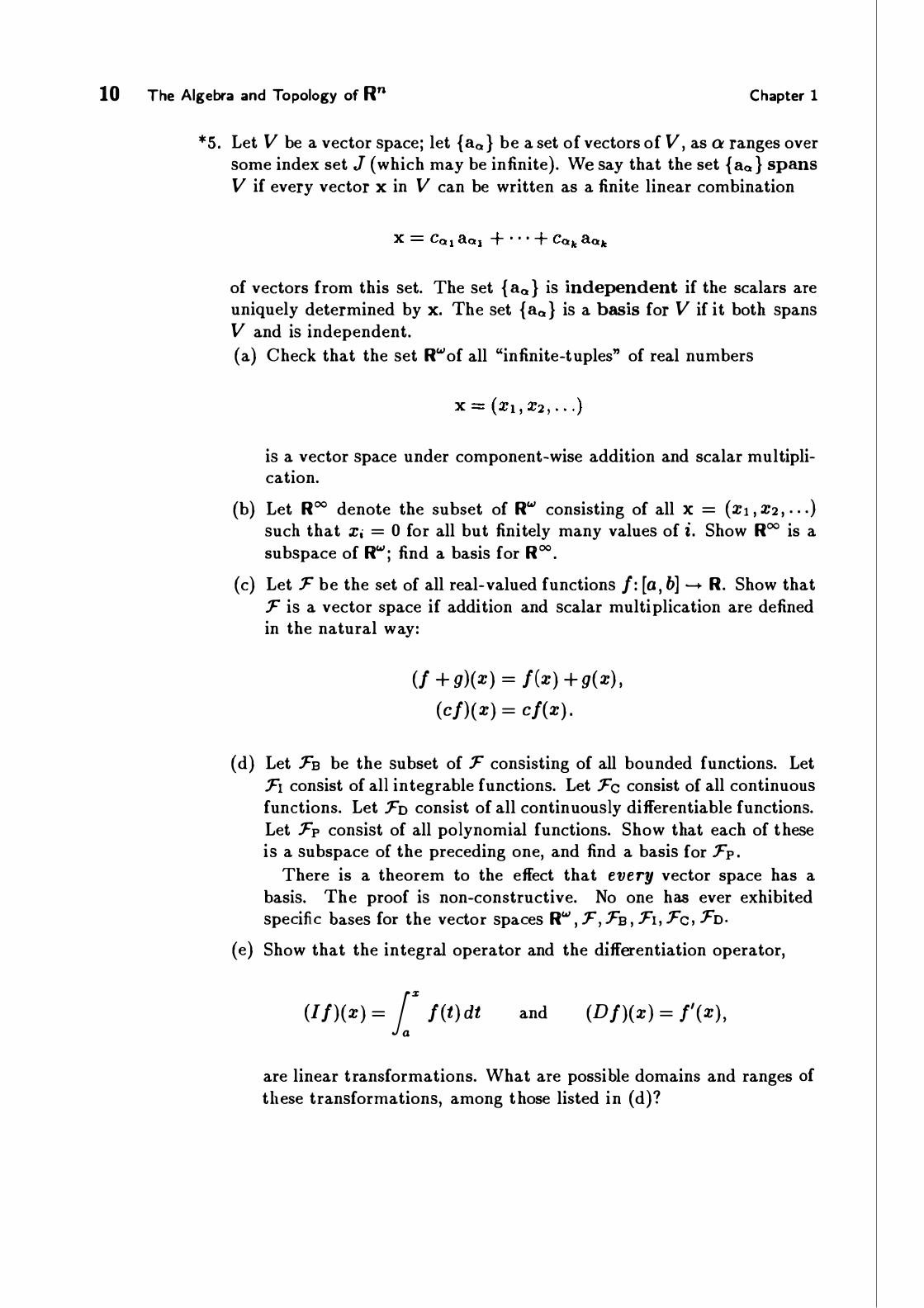
*5. Let V be a vector space; let { aQ} be a set of vectors of V, as a ranges over some index set J (which may be infinite). We say that the set { aQ} spans V if every vector x in V can be written as a finite linear combination
of vectors from this set. The set { aQ} is independent if the scalars are uniquely determined by x. The set {aQ} is a basis for V if it both spans V and is independent. (a) Check that the set Rwof all "infinite-tuples" of real numbers
is a vector space under component-wise addition and scalar multiplication.
(b) Let R00 denote the subset of Rw consisting of all X = (x1 ,X2 , . . . ) such that X; = 0 for all but finitely many values of i. Show R00 is a subspace of Rw; find a basis for R00•
(c) Let :F be the set of all real-valued functions f: [a, b] -+ R. Show that :F is a vector space if addition and scalar multiplication are defined in the natural way:
(f + g)(x) = f(x) + g(x),
( cf)(x) = cf(x).
(d) Let :FB be the subset of :F consisting of all bounded functions. Let :Fr consist of all integrable functions. Let :Fe consist of all continuous functions. Let :Fo consist of all continuously differentiable functions. Let :Fp consist of all polynomial functions. Show that each of these is a subspace of the preceding one, and find a basis for :Fp.
There is a theorem to the effect that every vector space has a basis. The proof is non-constructive. No one has ever exhibited specific bases for the vector spaces Rw , :F, :FB, :Fr, :Fe, :Fo.
(e) Show that the integral operator and the differentiation operator,
(If)(x) = 1"' f(t)d t and (Df)(x) = /'(x),
are linear transformations. What are possible domains and ranges of these transformations, among those listed in (d)?

§2. Matrix Inversion and Determinants 11
§2 . MATRIX I NVERS ION AND DETER M I NANTS
We now treat several further aspects of linear algebra. They are the following: elementary matrices, matrix inversion, and determinants. Proofs are included, in case some of these results are new to you.
Elementary matrices
D efinition. An el em entary matrix of size n by n is the matrix obtained by applying one of the elementary row operations to the identity matrix In .
The elementary matrices are of three basic types, depending on which of the three operations is used. The elementary matrix corresponding to the first elementary operation has the form
1
1
0
E =
1
1
0 1
1
• • row �2
The elementary matrix corresponding to the second elementary row operation has the form
1 1
1 c
E' =
0 1
1 1

12 The Algebra and Topology of Rn Chapter 1
And the elementary matrix corresponding to the third elementary row operation has the form
1
1
E"== .
'\._ row z .
1
1
One has the following basic result:
Th eor em 2.1. Let A be an n by m matrix. Any elementary row operation on A may be carried out by premultiplying A by the corresponding elementary matrix.
Proof. One proceeds by direct computation. The effect of multiplying A on the left by the matrix E is to interchange rows i1 and i2 of A. Similarly, multiplying A by E' has the effect of replacing row i 1 by itself plus c times row i2• And multiplying A by E" has the effect of multiplying row i by A. D
We will use this result later on when we prove the change of variables theorem for a multiple integral , as well as in the present sec tion.
The inverse of a matrix
D efinition. Let A be a matrix of size n by m; let B and C be matrices of size m by n. We say that B is a l eft inv ers e for A if B · A == Im, and we say that C is a right inv ers e for A if A · C =In .
Th eor em 2.2 . If A has both a left inverse B and a right inverse C, then they are unique and equal.
Proof. Equality follows from the computation
C = Im · C = (B · A) · C = B · (A · C) = B ·In = B.
If B1 is another left inverse for A, we apply this same computation with B1 replacing B. We conclude that C = B 1; thus B1 and B are equal . Hence B is unique. A similar computation shows that C is unique. D

§2. Matrix Inversion and Determinants
D efinit ion. If A has both a right inverse and a left inverse, then A is said to be invertibl e. The unique matrix that is both a right inverse and a left inverse for A is called the invers e of A, and is denoted A - I .
A necessary and sufficient condition for A to be invertible is that A be square and of maximal rank. That is the substance of the following two theorems:
Th eor em 2 .3 . Let A be a matrix of size n by m. If A is invertible, then
n = m = rank A.
Proof. Step 1. We show that for any k by n matrix D,
rank (D · A) < rank A.
The proof is easy. If R is a row matrix of size 1 by n, then R · A is a row matrix that equals a linear combination of the rows of A, so it is an element of the row space of A. The rows of D · A are obtained by multiplying the rows of D by A. Therefore each row of D · A is an element of the row space of A. Thus the row space of D · A is contained in the row space of A and our inequality follows.
Step 2. We show that if A has a left inverse B, then the rank of A equals the number of columns of A.
The equation Im = B · A implies by Step 1 that m = rank (B · A) < rank A. On the other hand, the row space of A is a subspace of m-tuple space, so that rank A < m.
Step 3. We prove the theorem. Let B be the inverse of A. The fact that B is a left inverse for A implies by Step 2 that rank A = m. The fact that B is a right inverse for A implies that
whence by Step 2, rank A = n. D
We prove the converse of this theorem in a slightly strengthened version:
Th eor em 2 .4. Let A be a matrix of size n by m. Suppose
n = m =rank A.
Then A is invertible; and furthermore, A equals a product of elementary matrices.
13

14 Tne Algebra and Topology of Rn Cnapter 1
Proof. Step 1. We note first that every elementary matrix is invertible, and that its inverse is an elementary matrix. This follows from the fact that elementary operations are invertible. Alternatively, you can check directly that the matrix E corresponding to an operation of the first type is its own inverse, that an inverse for E' can be obtained by replacing c by -c in the formula for E', and that an inverse for E" can be obtained by replacing A by 1/ A in the formula for E".
Step 2. We prove the theorem. Let A be an n by n matrix of rank n. Let us reduce A to reduced echelon form C by applying elementary row operations. Because C is square and its rank equals the number of its rows, C must equal the identity matrix In. It follows from Theorem 2 . 1 that there is a sequence E1, . . . , Ek of elementary matrices such that
If we multiply both sides of this equation on the left by E;; 1 , then by E;;! 1 , and so on , we obtain the equation
A - E-1 E-1 E-1. - 1 ' 2 "' k '
thus A equals a product of elementary matrices. Direct computation shows that the matrix
is both a right and a left inverse for A. D
One very useful consequence of this theorem is the following:
Theorem 2.5. If A is a square matrix and if B is a left inverse for A , then B is also a right inverse for A.
Proof. Since A has a left inverse, Step 2 of the proof of Theorem 2.3 implies that the rank of A equals the number of columns of A. Since A is square, this is the same as the number of rows of A, so the preceding theorem implies that A has an inverse. By Theorem 2.2 , this inverse must be B. D
An n by n matrix A is said to be singular if rank A < n; otherwise, it is said to be non-singular. The theorems just proved imply that A is invertible if and only if A is non-singular.
Determinants
The determinant is a function that assigns, to each square matrix A , a number called the determinant of A and denoted det A.

§2. Matrix Inversion and Determinants
The notation IAI is often used for the determinant of A, but we are using this notation to denote the sup norm of A. So we shall use "det A" to denote the determinant instead.
In this section, we state three axioms for the determinant function, and we assume the existence of a function satisfying these axioms. The actual construction of the general determinant function will be postponed to a later chapter.
D efin ition . A function that assigns , to each n by n matrix A, a real number denoted det A, is called a d et erminant function if it satisfies the following axioms:
( 1 ) If B is the matrix obtained by exchanging any two rows of A, then det B = - det A.
(2) Given i, the function det A is linear as a function of the ith row alone. ( 3) det In = 1 .
Condition (2) can be formulated as follows : Let i be fixed . Given an n-tuple x, let A; (x) denote the matrix obtained from A by replacing the ith row by x. Then condition (2) states that
det A;( ax + by) = a det A; (x) + b det A; (y).
These three axioms characterize the determinant function uniquely, as we shall see.
EXAMPLE 1. In low dimensions, it is easy to construct the determinant function. For 1 by 1 matrices, the function
det [a] = a
will do. For 2 by 2 matrices, the function
det [ � �] = ad - be suffices. And for 3 by 3 matrices, the function
will do, as you can readily check. For matrices of larger size, the definition is more complicated. For example, the expression for the determinant of a 4 by 4 matrix involves 24 terms; and for a 5 by 5 matrix, it involves 120 terms! Obviously, a less direct approach is needed. We shall return to this matter in Chapter 6.
Using the axioms , one can determine how the elementary row operations affect the value of the determinant . One has the following result:
15

16 The Algebra and Topology of Rn
Th eor em 2.6. Let A be an n by n matrix.
Chapter 1
(a) If E is the elementary matrix corresponding to the operation that exchanges rows i 1 and i2, then det(E · A) = - det A .
(b) If E' is the elementary matrix corresponding to the operation that replaces row i 1 of A by itself plus c times row i2 , then det(E' ·A) = det A .
(c) If E" is the elementary matrix corresponding to the operation that multiplies row i of A by the non-zero scalar A, then det(E" · A) = A(det A) .
(d) If A is the identity matrix In, then det A= 1 .
Proof. Property (a) is a restatement of Axiom 1 , and (d) is a restatement of Axiom 3. Property (c) follows directly from linearity (Axiom 2); it states merely that
det A; (Ax) = A(det A;(x)).
Now we verify (b). Note first that if A has two equal rows, then det A = 0 . For exchanging these rows does not change the matrix A, but by Axiom 1 it changes the sign of the determinant . Now let E' be the elementary operation that replaces row i = i1 by itself plus c times row i2. Let x equal row i1 and let y equal row i2 . We compute
det(E' · A)= det A; (x + cy) = det A; (x) + c det A;(y) = det A; (x) , since A; (y) has two equal rows,
= det A , since A;(x) = A. D
The four properties of the determinant function stated in this theorem are what one usually uses in practice rather than the axioms themselves. They also characterize the determinant completely, as we shall see.
One can use these properties to compute the determinants of the elementary matrices . Setting A = In in Theorem 2.6, we have
det E = -1 and det E' = 1 and det E" = A.
We shall see later how they can be used to compute the determinant in general . Now we derive the further properties of the determinant function that we
shall need.
Th eo rem 2 . 7 . Let A be a square matrix. If the rows of A are independent, then det A :f. 0; if the rows are dependent, then det A = 0 . Thus an n by n matrix A has rank n if and only if det A :f. 0.

§2. Matrix Inversion and Determinants
Proof. First, we note that if the ith row of A is the zero row, then det A = 0 . For multiplying row i by 2 leaves A unchanged; on the other hand, it must multiply the value of the determinant by 2 .
Second, we note that applying one of the elementary row operations to A does not affect the vanishing or non-vanishing of the determinant, for it alters the value of the determinant by a factor of either -1 or 1 or A (where A :f. 0).
Now by means of elementary row operations , let us reduce A to a matrix B in echelon form. (Elementary operations of types (1) and (2) will suffice.) If the rows of A are dependent, rank A < n; then rank B < n, so that B must have a zero row. Then det B = 0, as just noted; it follows that det A = 0 .
If the rows of A are independent, let us reduce B further to echelon form C . Since C is square and has rank n, C must equal the identity matrix In. Then det C :f. 0; it follows that det A :f. 0 . D
The proof just given can be refined so as to provide a method for calculating the determinant function:
Theor em 2 .8. Given a square matrix A, let use reduce it to echelon form B by elementary row operations of types {1} and {2). If B has a zero row, then det A = 0. Otherwise, let k be the number of row exchanges involved in the reduction process. Then det A equals ( -1 )k times the product of the diagonal entries of B.
Proof. If B has a zero row, then rank A < n and det A = 0 . So suppose that B has no zero row. We know from (a) and (b) of Theorem 2.6 that det A = ( -1 )k det B. Furthermore, B must have the form
B= '
0 0
where the diagonal entries are non-zero. It remains to show that
For that purpose, let us apply elementary operations of type (2) to make the entries above the diagonal into zeros. The diagonal entries are unaffected by the process ; therefore the resulting matrix has the form
0 0
17
18 Tne Algebra and Topology of Rn Cnapter 1
Since only operations of type (2) are involved, we have det B = det C . Now let us multiply row 1 of C by 1 /b 1 1 , row 2 by 1/b22 , and so on, obtaining as our end result the identity matrix In. Property (c) of Theorem 2.6 implies that
det In = (1 /bn) (1/b22) · · · (1/bnn ) det C,
so that (using property (d))
as desired. D
Corollary 2.9 . The determinant function is uniquely character-ized by its three axioms. It is also characterized by the four properties listed in Theorem 2.6.
Proof. The calculation of det A just given uses only properties (a)-( d) of Theorem 2.6 . These in turn follow from the three axioms. D
Theor em 2.10. Let A and B be n by n matrices. Then
det(A · B)= (det A) · (det B).
Proof. Step 1. The theorem holds when A is an elementary matrix. Indeed :
det(E · B) = - det B = (det E) (det B ) , det( E' . B) = det B = ( det E') ( det B) , det(E" · B) = .X • det B = ( det E") ( det B) .
Step 2. The theorem holds when rank A = n. For in that case, A is a product of elementary matrices, and one merely applies Step 1 repeatedly. Specifically, if A = E1 · · · Ek > then
det(A · B) = det(E1 · · · Ek · B)
= (det E1) det (E2 · · · Ek · B)
= (det E1) (det E2) · · · (det Ek ) (det B).
This equation holds for all B . In the case B = In , it tells us that
det A= (det E1) (det E2) · · · (det Ek )·
The theorem follows.

§2. Matrix Inversion and Determinants
Step 3. We complete the proof by showing that the theorem holds if rank A < n. We have in general,
rank (A · B) = rank (A · B)tr = rank (Btr · Atr) < rank Atr,
where the inequality follows from Step 1 of Theorem 2.3 . Thus if rank A < n, the theorem holds because both sides of the equation vanish. D
Even in low dimensions, this theorem would be very unpleasant to prove by direct computation. You might try it in the 2 by 2 case!
Th eor em 2 .11. det Atr = det A .
Proof. Step 1. We show the theorem holds when A is an elementary matrix.
Let E, E', and E" be elementary matrices ofthe three basic types . Direct inspection shows that Etr = E and (E")tr = E", so the theorem is trivial in these cases. For the matrix E' of type (2) , we note that its transpose is another elementary matrix of type (2), so that both have determinant 1 .
Step 2. We verify the theorem when A has rank n. In that case, A is a product of elementary matrices, say
Then
det Atr = det(Et · · · E�r ·En
= ( det Elr) · · · ( det E�r) ( det Efr) = (det EJ.:) · · · (det E2) (det E1) = ( det E1) ( det E2) · · · ( det Eli:)
= det(E1 · E2 · · · Ek) = det A .
by Theorem 2 .10 ,
by Step 1 ,
Step 3. The theorem holds if rank A < n . In this case, rank A tr < n, so that det Atr = 0 = det A . D
A formula for A - 1
We know that A is invertible if and only if det A :f. 0. Now we derive a formula for A - 1 that involves determinants explicitly.
D efin ition. Let A be an n by n matrix. The matrix of size n - 1 by n - 1 that is obtained from A by deleting the ith row and the ph column of A is called the (i, j)-m inor of A. It is denoted A;j. The number
( -1 )i+i det A;i
is called the (i ,j )-cofactor of A.
19

20 Tne Algebra and Topology of Rn Cnapter 1
L emma 2 . 12. Let A be an n by n matrix; let b denote its entry in row i and column j.
(a) If all the entries in row i other than b vanish, then
det A = b(-1)i+i det Aij ·
(b) The same equation holds if all the entries in column j other than the entry b vanish.
Proof. Step 1. We verify a special case of the theorem. Let b, a2, . . • , an be fixed numbers . Given an n - 1 by n - 1 matrix D, let A(D) denote the n by n matrix
b 0
A(D) =
0
We show that det A( D) = b(det D) .
a2 . . .
D
an ·
If b = 0, this result is obvious, since in that case rank A(D) < n. So assume b :f. 0. Define a function f by the equation
f(D) = (1 /b) det A(D).
We show that f satisfies the four properties stated in Theorem 2.6 , so that f(D) = det D.
Exchanging two rows of D has the effect of exchanging two rows of A( D), which changes the value of f by a factor -1 . Replacing row i1 of D by itself plus c times row i2 of D has the effect of replacing row (i 1 + 1 ) of A(D) by itself plus row (i2 + 1 ) of A(D), which leaves the value of f unchanged. Multiplying row i of D by A has the effect of multiplying row (i + 1 ) of A( D) by A, which changes the value of f by a factor of A. Finally, if D = In-l, then A(D) is in echelon form, so det A(D) = b · 1 · · · 1 by Theorem 2.8, and f(D) = 1 .
Step 2. It follows by taking transposes that
b a2
det . . an
0 . . .
D
0
= b(det D).
Step 3. V\Te prove the theorem. Let A be a matrix satisfying the hypotheses of our theorem. One can by a sequence of i - 1 exchanges of adjacent

§2 . Matrix Inversion and Determinants
rows bring the ith row of A up to the top of matrix, without affecting the order of the remaining rows . Then by a sequence of j - 1 exchanges of adjacent columns, one can bring the ph column of this matrix to the left edge of the matrix, without affecting the order of the remaining columns. The matrix C that results has the form of one of the matrices considered in Steps 1 and 2 . Furthermore, the ( 1 , 1 )-minor C1 ,1 of the matrix C is identical with the (i ,j)-minor A; i of the original matrix A.
Now each row exchange changes the sign of the determinant . So does each column exchange, by Theorem 2 . 1 1 . Therefore
Thus
det C = ( -1 ) (i-1 )+(j -1 ) det A = ( -1) i+i det A.
det A= ( -1)i+J det C,
= ( -1) i+i b det C1 ,1 by Steps 1 and 2,
= (-1 )i +ibdet A; i· D
Theorem 2.13 (Cramer's rule ) . Let A be an n by n matrix with successive columns a1, ... , an . Let
x = and c =
be column matrices. If A · x = c, then
• . •
(det A) · X; = det [a1 · · ·a; -1 c a i+1 ···an] ·
Proof. Let e1 , ... , en be the standard basis for Rn , where each e; IS written as a column matrix. Let C be the matrix
The equations A · ej = aj and A · x = c imply that
By Theorem 2 .10,
(det A) · (det C)= det [a1 · .. a ;-1 c a; +1 .. ·an] ·
21

22 The Algebra and Topology of Rn
Now C has the form
C=
1
0
0
Chapter 1
0
X; 0 '
1
where the entry x; appears in row i and column i . Hence by the preceding lemma,
det C = x; (-1)i+i det In -1 = X;. The theorem follows. D
Here now is the formula we have been seeking:
Th eor em 2.14. Let A be an n by n matrix of rank n; let B = A -1 . Then
_ (-1 )i+idet Aji b;i - det A ·
Proof. Let j be fixed throughout this argument . Let
x =
denote the ph column of the matrix B. The fact that A · B = In implies in particular that A · x = ei. Cramer's rule tells us that
(det A) · X; = det [a1 · · · ai-1 ej Ri+I ···an] ·
We conclude from Lemma 2 . 12 that
Since x; = b;i, our theorem follows. D
This theorem gives us an algorithm for computing the inverse of a matrix A. One proceeds as follows :
( 1 ) First, form the matrix whose entry in row i and column j is ( -1 )i+i det A;i; this matrix is called the matrix of cofactors of A.
(2) Second , take the transpose of this matrix. (3) Third, divide each entry of this matrix by det A.

§2. Matrix Inversion and Determinants
This algorithm is in fact not very useful for practical purposes; computing determinants is simply too time-consuming. The importance of this formula for A -1 is theoretical, as we shall see. If one wishes actually to compute A -1, there is an algorithm based on Gauss-Jordan reduction that is more efficient. It is outlined in the exercises.
Expansion by cofactors
We now derive a final formula for evaluating the determinant. This is the one place we actually need the axioms for the determinant function rather than the properties stated in Theorem 2.6.
Theor em 2 .15 . Let A be an n by n matrix. Let i be fixed. Then
n ""' . k det A = L.) -1 )'+ a; k · det A; k. k =1
Here A;k is, as usual, the (i , k)-minor of A. This rule is called the "rule for expansion of the determinant by cofactors of the ith row." There is a similar rule for expansion by cofactors of the ph column, proved by taking transposes.
Proof. Let A;(x) , as usual, denote the matrix obtained from A by replacing the ith row by the n-tuple x. If e1 , . . . , en denote the usual basis vectors in R " (written as row matrices in this case) , then the ith row of A can be written in the form
Then n
det A= L a;k · det A;( ek) k =1
by linearity (Axiom 2),
by Lemma 2 .12 . D
23

24 Tne Algebra and Topology of Rn
EXERCISES
1 . Consider the matrix
A= [ � -n . (a) Find two different left inverses for A. (b) Show that A has no right inverse.
2. Let A be an n by m matrix with n =I= m.
Cnapter 1
(a) If rank A = m, show there exists a matrix D that is a product of elementary matrices such that
(b) Show that A has a left inverse if and only if rank A= m. (c) Show that A has a right inverse if and only if rank A= n.
3. Verify that the functions defined in Example 1 satisfy the axioms for the determinant function.
4. (a) Let A be an n by n matrix of rank n . By applying elementary row operations to A, one can reduce A to the identity matrix. Show that by applying the same operations, in the same order, to In , one obtains the matrix A -1.
(b) Let 1 2 3
A= o 1 2
1 2 1
Calculate A -1 by using the algorithm suggested in (a). [Hin t: An easy way to do this is to reduce the 3 by 6 matrix [ A 13 ] to reduced echelon form.]
(c) Calculate A -1 using the formula involving determinants. 5. Let
where ad- be =I= 0. Find A -1•
*6. Prove the following:
Theorem. Le t A be a k by k matrix, let D have size n by n and le t C have size n by k. Then
det [� �] =(det A)·(det D).

§3.
Proof. First show that
Review of Topology in Rn 25
[A o ] · [lk O ] = [A o ] · o In C D C D
Then use Lemma 2 .12 .
§3. REVIEW OF TOPOLOGY IN Rn
Metric spaces
Recall that if A and B are sets , then A x B denotes the set of all ordered pairs (a, b) for which a E A and b E B .
Given a set X, a metric on X is a function d : X x X -+ R such that the following properties hold for all X, y, z E X:
(1) d(x , y) = d(y, x ) . (2) d(x , y) > 0, and equality holds if and only if X = y. (3) d(x, z) < d(x, y) + d(y, z).
A metric space is a set X together with a specific metric on X. We often suppress mention of the metric, and speak simply of "the metric space X."
If X is a metric space with metric d, and if Y is a subset of X, then the restrict ion of d to the set Y x Y is a metric on Y; thus Y is a metric space in its own right . It is called a subspac e of X.
For example, Rn has the metrics
d(x, y) = II x - Y I I and d(x, y) = l x - y l ;
they are called the euclidean metric and the sup metric, respectively. It follows immediately from the properties of a norm that they are metrics . For many purposes, these two metrics on Rn are equivalent , as we shall see.
We shall in this book be concerned only with the metric space Rn and its subspaces, except for the expository final section, in which we deal with general metric spaces . The space Rn is commonly called n-dimensional euclidean space .
If X is a metric space with metric d, then given x0 E X and given f > 0, the set
U(xo ; E) = {x I d(x , xo) < E}

26 Tne Algebra and Topology of Rn Cnapter 1
is called the f-n eighborhood of x0 , or the f-n eighborhood c ent ered at x0 . A subset U of X is said to be op en in X if for each x0 E U there is a corresponding f > 0 such that U ( x0 ; E) is contained in U. A subset C of X is said to be closed in X if its complement X - C is open in X. It follows from the triangle inequality that an f-neighborhood is itself an open set.
If U is any open set containing x 0 , we commonly refer to U simply as a n eighborhood of x0.
Theor em 3.1 . Let (X, d) be a metric space. Then finite intersec-tions and arbitrary unions of open sets of X are open in X. Similarly, finite unions and arbitrary intersections of closed sets of X are closed in X. D
Theor em 3.2. Let X be a metric space; let Y be a subspace. A subset A of Y is open in Y if and only if it has the form
A = U n Y,
where U is open in X. Similarly, a subset A of Y is closed in Y if and only if it has the form
where C is closed in X. D
A = C n Y,
It follows that if A is open in Y and Y is open in X, then A is open in X. Similarly, if A is closed in Y and Y is closed in X, then A is closed in X.
If X is a metric space, a point x0 of X is said to be a limit point of the subset A of X if every f-neighborhood of x0 intersects A in at least one point different from x0. An equivalent condition is to require that every neighborhood of x0 contain infinitely many points of A.
Th eorem 3 .3. If A is a subset of X, then the set A consisting of A and all its limit points is a closed set of X. A subset of X is closed if and only if it contains all its limit points. D
The set A is called the closure of A. In Rn, the f-neighborhoods in our two standard metrics are given special
names. If a E Rn , the f-neighborhood of a in the euclidean metric is called the op en ball of radius f centered at a, and denoted B(a; E) . The f-neighborhood of a in the sup metric is called the op en cub e of radius f centered at a, and denoted C( a; E) . The inequalities I x I < I I x I I < fo I x I lead to the following inclusions:
B(a; E) C C(a; E) C B(a; Vn E) .
These inclusions in turn imply the following:

§3. Review of Topology in R" 27
Th eor em 3 .4 . If X is a subspace of R", the collection of open sets of X is the same whether one uses the euclidean metric or the sup metric on X. The same is true for the collection of closed sets of X. D
In general, any property of a metric space X that depends only on the collection of open sets of X, rather than on the specific metric involved, is called a topological prop erty of X. Limits, continuity, and compactness are examples of such, as we shall see.
Limits and Continuity
Let X and Y be metric spaces, with metrics dx and dy , respectively. We say that a function f : X -+ Y is continuous at th e point x0 of X
if for each open set V of Y containing f(xo) , there is an open set U of X containing Xo such that f ( U) C lf. We say f is continuous if it is continuous at each point x0 of X. Continuity of f is equivalent to the requirement that for each open set V of Y, the set
f- 1 (V) = {x I f(x) E V}
is open in X, or alternatively, the requirement that for each closed set D of Y, the set f- 1(D) is closed in X.
Continuity may be formulated in a way that involves the metrics specifically. The function f is continuous at x0 if and only if the following holds: For each f > 0, there is a corresponding 8 > 0 such that
dy(f(x), f(xo)) < f whenever dx (x, xo) < 8. This is the classical "E-8 formulation of continuity."
Note that given Xo E X it may happen that for some 8 > 0, the 8-neighborhood of x0 consists of the point x0 alone. In that case, x0 is called an isolated point of X , and any function f : X -+ Y is automatically continuous at Xo!
A constant function from X to Y is continuous, and so is the identity function ix : X -+ X. So are restrictions and composites of continuous functions:
Theor em 3.5. (a) Let Xo E A, where A is a subspace of X. If f : X -+ Y is continuous at xo, then the restricted function f I A : A -+ Y is continuous at x0 .
(b) Let f : X -+ Y and g : Y -+ Z. If f is continuous at x0 and g is continuous at Yo = f(x0), then g o f : X -+ Z is continuous at x0 . D
Theor em 3.6. the form
(a) Let X be a metric space. Let f : X -+ R" have
f(x) = (f1 (x), . . . , fn(x)) .

28 Tne Algebra and Topology of Rn Cnapter 1
Then f is continuous at Xo if and only if each function f; : X -+ R is continuous at x 0 . The functions f; are called the compon ent functions of f.
(b) Let f, g : X -+ R be continuous at x0 . Then f + g and f - g and f · g are continuous at xo; and f/g is continuous at Xo if g(x0 ) :f. 0 .
(c) The projection function 11"; : Rn -+ R given by 1r; (x) = x; is con-tinuous. D
These theorems imply that funct ions formed from the familiar real-valued continuous functions of calculus , using algebraic operations and composites, are continuous in Rn . For instance, since one knows that the functions f'l' and sin x are continuous in R , it follows that such a function as
f(s, t, u , v) = (sin(s + t))/eu v
is continuous in R4. Now we define the notion of limit. Let X be a metric space . Let A C X
and let f : A -+ Y . Let x0 be a limit point of the domain A of f. (The point Xo may or may not belong to A.) We say that f(x) approaches Yo as x approaches x0 if for each open set V of Y containing y0 , there is an open set U of X containing x0 such that f(x) E V whenever x is in U n A and x :f. Xo . This statement is expressed symbolically in the form
f(x) -+ Yo as x -+ Xo.
We also say in this situation that the limit of f(x), as X approaches Xo, is y0 . This statement is expressed symbolically by the equation
lim f(x) = Yo · X -+ X o
Note that the requirement that x0 be a limit point of A guarantees that there exist points X different from Xo belonging to the set u nA. We do not attempt to define the limit of f if Xo is not a limit point of the domain of f.
Note also that the value of f at Xo (provided f is even defined at xo) is not involved in the definition of the limit .
The notion of limit can be formulated in a way that involves the metrics specifically. One shows readily that f(x) approaches y0 as x approaches x0 if and only if the following condition holds: For each f > 0, there is a corresponding b > 0 such that
dy (f(x) , Yo) < f whenever x E A and 0 < dx (x, x0) < o.
There is a direct relation between limits and continuity; it is the following:

§3. Review of Topology in Rn 29
Theorem 3 . 7. Let f : X -+ Y. If Xo is an isolated point of X, then f is continuous at x0 • Otherwise, f is continuous at x0 if and only if f(x) -+ f(xo) as x -+ Xo . D
Most of the theorems dealing with continuity have counterparts that deal with limits:
Theorem 3 .8 . (a) Let A C X; let f : A -+ Rn have the form
f(x) = (f1 (x), . . . , fn (x)).
Let a = (a1 , . . . , an ) · Then f(x) -+ a as x -+ Xo if and only if f; (x) -+ a; as x -+ xo, for each i.
(b) Let f, g : A -+ R . If f(x) -+ a and g(x ) -+ b as x -+ xo, then as X -+ Xo,
f(x) + g(x) -+ a + b, f(x) - g(x) -+ a - b, f(x) · g(x) -+ a · b ;
also, f(x)jg(x) -+ ajb if b f: 0 . D
Interior and Exterior
The following concepts make sense in an arbitrary metric space. Since we shall use them only for Rn , we define them only in that case.
Definition . Let A be a subset of R". The interior of A, as a subset of R", is defined to be the union of all open sets of Rn that are contained in A; it is denoted Int A. The exterior of A is defined to be the union of all open sets of R" that are disjoint from A; it is denoted Ext A. The boundary of A consists of those points of R" that belong neither to Int A nor to Ext A ; it is denoted Bd A.
A point x is in Bd A if and only if every open set containing x intersects both A and the complement Rn - A of A. The space Rn is the union of the disjoint sets Int A, Ext A, and Bd A; the first two are open in Rn and the third is closed in Rn .
For example, suppose Q is the rectangle
consisting of all points x of R" such that a; < X; < b; for all i . You can check that

30 Tne Algebra and Topology of Rn Cnapter 1
We often call Int Q an open rectangle. Furthermore, Ext Q = Rn - Q and Bd Q = Q - Int Q.
An open cube is a special case of an open rectangle; indeed,
The corresponding (closed) rectangle
is often called a closed cube, or simply a cube, centered at a.
EXERCISES
Throughout, let X be a metric space with metric d . 1 . Show that U(x0; E) is an open set.
2 . Let Y C X. Give an example where A is open in Y but not open in X. Give an example where A is closed in Y but not closed in X.
3. Let A C X. Show that if C is a closed set of X and C contains A, then C contains A.
4. (a) Show that if Q is a rectangle, then Q equals the closure of Int Q.
(b) If D is a closed set, what is the relation in general between the set D and the closure of Int D?
(c) If U is an open set,�hat is the relation in general between the set U and the interior of U?
5. Let I : X -+ Y. Show that I is continuous if and only if for each x E X there is a neighborhood U of x such that I I U is continuous.
6. Let X = A U B, where A and B are subspaces of X. Let I : X -+ Y; suppose that the restricted functions
I I A: A -+ Y and I I B : B -+ Y
are continuous. Show that if both A and B are closed in X, then I is continuous.
7. Finding the limit of a composite function g o I is easy if both I and g are continuous; see Theorem 3.5. Otherwise, it can be a bit tricky:
Let I : X -+ Y and g : Y -+ Z. Let Xo be a limit point of X and let Yo be a limit point of Y. See Figure 3.1 . Consider the following three conditions:
(i) l(x) -+ Yo as X -+ Xo.
(ii) g(y) -+ Zo as y -+ Yo ·
(iii) g(f(x)) -+ Zo as x -+ Xo.
(a) Give an example where (i) and (ii) hold, but (iii) does not. (b) Show that if (i) and (ii) hold and if g(yo ) = Zo, then (iii) holds.

§3. Review of Topology in Rn 31
8 . Let I : R -+ R be defined by setting l(x) = sin x if x is rational, and l(x) = 0 otherwise. At what points is I continuous?
9. If we denote the general point of R2 by ( x, y), determine Int A, Ext A, and Bd A for the subset A of R2 specified by each of the following conditions:
(a) x = 0. (e) x and y are rational. (b) 0 < x < 1 . (f) 0 < x2 + y2 < 1. (c) 0 < x < 1 and 0 < y < 1 . (g) y < x2•
(d) x is rational and y > 0. (h) y < x2 •
� · x I • Xo -- · • y
Yo
Figure 3.1
g
y
• Zo

32 Tne Algebra and Topology of R" Cnapter 1
§4. CO MPACT SU BSPACES AND CONNECTED SU BS PACES OF R"
An important class of subs paces of R" is the class of compact spaces . We shall use the basic properties of such spaces constantly. The properties we shall need are summarized in the theorems of this section. Proofs are included, since some of these results you may not have seen before.
A second useful class of spaces is the class of connected spaces ; we summarize here those few propert ies we shall need.
We do not attempt to deal here with compactness and connectedness in arbitrary metric spaces, but comment that many of our proofs do hold in that more general situation.
Compact spaces
Definition. Let X be a subspace of R". A covering of X is a collection of subsets of R" whose union contains X; if each of the subsets is open in R", it is called an open covering of X. The space X is said to be compact if every open covering of X contains a finite subcollection that also forms an open covering of X.
While this definition of compactness involves open sets of R", it can be reformulated in a manner that involves only open sets of the space X:
Theorem 4 . 1. A subspace X of R" is compact if and only if for every collection of sets open in X whose union is X, there is a finite subcollection whose union equals X.
Proof. Suppose X is compact. Let {A a } be a collection of sets open in X whose union is X. Choose , for each a , an open set U a of R" such that Aa = Ua n X. Since X is compact, some finite subcollection of the collection { U a } covers X, say for a = a1 , . . . , ak . Then the sets A a , for a = a 1 , . . . , ak , have X as their union.
The proof of the converse is similar. D
The following result is always proved in a first course in analysis , so the proof will be omitted here:
Theorem 4.2. The subspace [a , b] of R is compact. D
Definition. A subspace X of R" is said to be bounded if there is an M such that I x I < M for all x E X.
We shall eventually show that a subspace of R" is compact if and only if it is closed and bounded . Half of that theorem is easy; we prove it now:
§4.
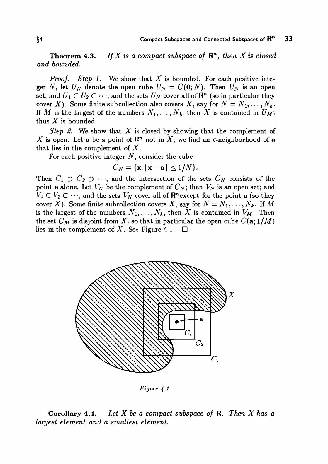
Theorem 4.3. and bounded.
Compact Subspaces and Connected Subspaces of Rn 33
If X is a compact subspace of Rn, then X is closed
Proof. Step 1. We show that X is bounded. For each positive integer N, let UN denote the open cube UN = e(o; N) . Then UN is an open set; and ul c u2 c . . · ; and the sets u N cover all of Rn (so in particular they cover X). Some finite subcollection also covers X, say for N = N11 . . . , Nk .
If M is the largest of the numbers N� , . . . , Nk, then X is contained in U M ; thus X is bounded.
Step 2. We show that X is closed by showing that the complement of X is open. Let a be a point of Rn not in X; we find an f-neighborhood of a that lies in the complement of X.
For each positive integer N , consider the cube
eN = {x; l x - a i < 1/N} .
Then el :) e2 :) . . · , and the intersection of the sets eN consists of the point a alone. Let VN be the complement of eN ; then VN is an open set; and vl c v2 c . . · ; and the sets VN cover all of Rnexcept for the point a (so they cover X). Some finite subcollection covers X, say for N = N1 1 . . . , Nk . If M
is the largest of the numbers Nb . . . , Nk , then X is contained in VM . Then the set eM is disjoint from X, so that in particular the open cube e(a; 1/M) lies in the complement of X. See Figure 4 . 1 . D
X
e.....i---+- a
Figure 4 . 1
Corollary 4.4. Let X be a compact subspace of R. Then X has a largest element and a smallest element.

34 The Algebra and Topology of R" Chapter 1
Proof. Since X is bounded, it has a greatest lower bound and a least upper bound. Since X is closed , these elements must belong to X. D
Here is a basic (and familiar) result that is used constantly:
Theorem 4.5 (Extreme-value theorem). Let X be a compact subspace of Rm . If f : X --+ R" is continuous, then f(X) is a compact subspace of R" .
In particular, if 1/J : X --+ R is continuous, then 1/J has a maximum value and a minimum value.
Proof. Let {Va} be a collection of open sets of R" that covers f(X). The sets f- 1 (Va) form an open covering of X. Hence some finitely many of them cover X, say for a = a 1 , . . . , ak. Then the sets Va for a = a1 , . . . , ak cover f(X). Thus f(X) is compact.
Now if 1/J : X --+ R is continuous, 1/J(X) is compact, so it has a largest element and a smallest element. These are the maximum and minimum values of 1/J. D
Now we prove a result that may not be so familiar.
Definition. Let X be a subset of R" . Given E > 0, the union of the sets B(a; E) , as a ranges over all points of X, is called the E-neighborhood of X in the euclidean metric. Similarly, the union of the sets C(a; E) is called the E-neighborhood of X in the sup metric.
Theorem 4.6 (The E-neighborhood theorem). Let X be a com-pact subspace of R" ; let U be an open set of R"containing X. Then there is an E > 0 such that the E-neighborhood of X (in either metric) is contained in U.
Proof. The E-neighborhood of X in the euclidean metric is contained in the E-neighborhood of X in the sup metric. Therefore it suffices to deal only with the latter case.
Step 1. Let C be a fixed subset of R" . For each x E R" , we define
d(x, C) = inf { I x - c I ; c E C}.
We call d(x, C) the distance from x to C. We show it is continuous as a function of x:
Let c E C; let x, y E R" . The triangle inequality implies that
d(x, C) - I x - y I < I x - c I - I x - y I < I y - c I ·

§4. Compact Subspaces and Connected Subspaces of Rn 35
This inequality holds for all c E C; therefore
d(x, C) - I x - y l < d(y, C) ,
so that d(x, C) - d(y, C) < I x - Y I ·
The same inequality holds if x and y are interchanged; continuity of d(x, C) follows.
Step 2. We prove the theorem. Given U, define f : X --+ R by the equation
f(x) = d(x, Rn - U) .
Then f is a continuous function. Furthermore, f(x) > 0 for all x E X. For if x E X, then some 15-neighborhood of x is contained in U, whence f(x) > 15. Because X is compact, f has a minimum value f. Because f takes on only positive values, this minimum value is positive. Then the f-neighborhood of X is contained in U. D
This theorem does not hold without some hypothesis on the set X . If X is the x-axis in R2, for example, and U is the open set
then there is no f such that the f-neighborhood of X is contained in U. See Figure 4.2 .
Figure 4.2
Here is another familiar result.
Theorem 4.7 (Uniform continuity). Let X be a compact subspace of Rm; let f : X --+ Rn be continuous. Given f > 0, there is a 15 > 0 such that whenever x, y E X,
l x - y I < 15 implies I f(x) - f(y) I < f .

36 The Algebra and Topology of Rn Chapter 1
This result also holds if one uses the euclidean metric instead of the sup metric.
The condition stated in the conclusion of the theorem is called the condition of uniform continuity.
Proof Consider the subspace X x X of Rm x Rm ; and within this, consider the space
� = { (x, x) l x E X } ,
which is called the diagonal of X x X. The diagonal is a compact subspace of R2m , since it is the image of the compact space X under the continuous map f(x) = (x, x).
We prove the theorem first for the euclidean metric. Consider the function g : X x X -+ R defined by the equation
g(x, y) = I I f(x) - f(y) I I ·
Then consider the set of points (x, y) of X x X for which g(x, y) < f. Because g is continuous, this set is an open set of X x X. Also, it contains the diagonal �' since g(x ,x) = 0. Therefore, it equals the intersection with X x X of an open set U of Rm x Rm that contains �. See Figure 4.3 .
X
X
.-'-- (x, y)
'.l.-J.- ( y' y)
Figure 4 .3
Compactness of � implies that for some b , the b-neighborhood of � is contained in U. This is the b required by our theorem. For if x, y E X with l l x - y l l < b, then
l l (x, y) - (y , y) l l = l l (x - y, O) I I = l l x - y l l < b,
so that (x,y) belongs to the b-neighborhood of the diagonal �. Then (x,y) belongs to U, so that g(x , y) < E, as desired .

§4. Compact Subs paces and Connected Subspaces of Rn 3 7
The corresponding result for the sup metric can be derived by a similar proof, or simply by noting that if I x - y I < b / fo, then I I x - y I I < b , whence
I f(x) - f(y) I < I I f(x) - f(y) I I < c o
To complete our characterization of the compact subspaces of Rn, we need the following lemma:
Lemma 4.8. The rectangle
Q = [a � , b i ] X · · · X [an, bn]
in Rn is compact.
Proof. We proceed by induction on n. The lemma is true for n = 1 ; we suppose it true for n - 1 and prove it true for n. We can write
where X is a rectangle in Rn- l . Then X is compact by the induction hypothesis. Let A be an open covering of Q.
Step 1. We show that given t E [an , bn] , there is an f > 0 such that the set
X X (t - f, t + E) can be covered by finitely many elements of A.
The set X x t is a compact subspace of Rn, for it is the image of X under the continuous map f : X -+ Rn given by f(x) = (x, t ) . Therefore it may be covered by finitely many elements of A, say by A1 , . . . , Ak .
Let U be the union of these sets ; then U is open and contains X x t. See Figure 4.4.
bn u
t ( p /LL/// �
X X t an
X
Figure 4.4
Because X x t is compact, there is an f > 0 such that the E-neighborhood of X x t is contained in U. Then in particular, the set X x (t - E, t + E) is contained in U, and hence is covered by A1 , . . . , Ak .

38 The Algebra and Topology of Rn Chapter 1
Step 2. By the result of Step 1 , we may for each t E [an , bn] choose an open interval Yt about t , such that the set X x Yt can be covered by finitely many elements of the collection A.
Now the open intervals Yt in R cover the interval [an , bn] ; hence finitely many of them cover this interval, say for t = t 1 , • • • , tm .
Then Q = X x [an , bn] is contained in the union of the sets X x Yt for t = t 1 , • • • , tm ; since each of these sets can be covered by finitely many elements of A, so may Q be covered. D
Theorem 4.9. If X is a closed and bounded subspace of Rn, then X is compact.
Proof. Let A be a collection of open sets that covers X. Let us adjoin to this collection the single set Rn - X, which is open in Rn because X is closed . Then we have an open covering of all of Rn . Because X is bounded, we can choose a rectangle Q that contains X; our collection then in particular covers Q.
Since Q is compact, some finite sub collection covers Q. If this finite subcollection contains the set Rn - X, we discard it from the collection. We then have a finite subcollection of the collection A; it may not cover all of Q, but it certainly covers X, since the set Rn - X we discarded contains no point of X. D
All the theorems of this section hold if Rn and Rm are replaced by arbitrary metric spaces, except for the theorem just proved. That theorem does not hold in an arbitrary metric space; see the exercises.
Connected spaces
If X is a metric space, then X is said to be connected if X cannot be written as the union of two disjoint non-empty sets A and B, each of which is open in X.
The following theorem is always proved in a first course in analysis, so the proof will be omitted here:
Theorem 4.10. The closed interval [a, b] of Rn is connected. D
The basic fact about connected spaces that we shall use is the following:
Theorem 4.1 1 (Intermediate-value theorem) . Let X be con-nected. If f : X -+ Y is continuous, then f(X) is a connected subspace of Y.
In particular, if 1/J : X -+ R is continuous and if f(xo) < r < f(x i ) for some points xa , x 1 of X, then f(x) = r for some point x of X.

§4. Compact Subspaces and Connected Subspaces of Rn 39
Proof. Suppose f(X) = A U B , where A and B are disjoint sets open in f(X) . Then j- 1 (A) and j- 1 (B) are disjoint sets whose union is X, and each is open in X because f is continuous. This contradicts connectedness of X.
Given 1/J, let A consist of all y in R with y < r, and let B consist of all y with y > r. Then A and B are open in R; if the set f(X) does not contain r, then f(X) is the union of the disjoint sets f(X) n A and f(X) n B, each of which is open in /(X). This contradicts connectedness of f(X) . D
If a and b are points of Rn , then the line segment joining a and b is defined to be the set of all points x of the form x = a + t(b - a) , where 0 < t < 1 . Any line segment is connected, for it is the image of the interval (0, 1] under the continuous map t --+ a + t(b - a) .
A subset A of Rn is said to be convex if for every pair a,b of points of A, the line segment joining a and b is contained in A. Any convex subset A of Rn is automatically connected: For if A is the union of the disjoint sets U
and V, each of which is open in A, we need merely choose a in U and b in V, and note that if L is the line segment joining a and b, then the sets U n L and V n L are disjoint, non-empty, and oper. in L.
It follows that in Rn all open balls and open cubes and rectangles are connected. (See the exercises .)
EXERCISES
1. Let R+ denote the set of positive real numbers.
(a) Show that the continuous function f : R+ -+ R given by /(x) = 1/(l+x) is bounded but has neither a maximum value nor a minimum value.
(b) Show that the continuous function g : R+ -+ R given by g(x) = sin( l/x) is bounded but does not satisfy the condition of uniform continuity on R+ .
2. Let X denote t he subset (-1, 1) x 0 of R2 , and let U be the open ball B(O; 1 ) in R2 , which contains X. Show there is no E > 0 such that the E-neighborhood of X in Rn is contained in U.
3 . Let R00 be the set of all "infinite- tuples" x = (x1 , x2 , • • • ) of real numbers that end in an infinite string of D's. (See the exercises of § 1 .} Define an inner product on R00 by the rule {x, y) = �x;y; . (This is a finite sum, since all but finitely many terms vanish.) Let II x - y II be the corresponding metric on R"". Define
e; = ( 0, . . . , 0, 1 , 0, . . . , 0 , . . . ) ,
where 1 appears in the i1h place. Then the e; form a basis for R00• Let X be the set of all the points e; . Show that X is closed , bounded, and non-compact.

40 The Algebra and Topology of Fil"
4. (a) Show that open balls and open cubes in Rnare convex.
(b) Show that (open and closed) rectangles in Rn are convex.
Chapter 1

Differentiation
In this chapter , we consider functions mapping Rm into Rn, and we define what we mean by the derivative of such a function. Much of our discussion will simply generalize facts that are already familiar to you from calculus.
The two major results of this chapter are the inverse function theorem, which gives conditions under which a differentiable function from Rn to Rn has a differentiable inverse, and the implicit function theorem, which provides the theoretical underpinning for the technique of implicit differentiation as studied in calculus.
Recall that we write the elements of Rm and Rn as column matrices unless specifically stated otherwise.
§5. THE DER IVATIVE
First, let us recall how the derivative of a real-valued function of a real variable is defined.
Let A be a subset of R; let 1/J : A -+ R . Suppose A contains a neighborhood of the point a. We define the derivative of 1/J at a by the equation
A..'( ) _ 1. 1/J( a + t) - 1/J( a) 'f' a - 1m ,
t-+0 t
provided the limit exists. In this case, we say that 1/J is differentiable at a . The following facts are an immediate consequence:
41

4 2 Differentiation Chapter 2
( 1) Differentiable functions are continuous. (2) Composites of differentiable functions are differentiable.
We seek now to define the derivative of a function f mapping a subset of Rm into R". We cannot simply replace a and t in the definition just given by points of Rm , for we cannot divide a point of R" by a point of Rm if m > 1 ! Here is a first attempt at a definition:
Definition. Let A C Rm; let J : A --+ R". Suppose A contains a neighborhood of a. Given u E Rm with u ::p 0 , define
!'(a· u) = lim f(a + tu) - f(a)
' t-+0 t '
provided the limit exists. This limit depends both on a and on u; it is called the directional derivative of f at a with respect to the vector u. (In calculus, one usually requires u to be a unit vector , but that is not necessary.)
EXAMPLE 1 . Let I : R2 -+ R be given by the equation
The directional derivative of I at a = ( a1 , a2 ) with respect to the vector u = (l , O) is
With respect to the vector v = ( 1 , 2), the directional derivative is
It is tempting to believe that the "directional derivative" is the appropriate generalization of the notion of "derivative," and to say that f is differentiable at a if f'(a; u) exists for every u ::p 0. This would not , however , be a very useful definition of differentiability. It would not follow, for instance, that differentiability implies continuity. (See Example 3 following.) Nor would it follow that composites of differentiable functions are differentiable. (See the exercises of § 7 .) So we seek something stronger .
In order to motivate our eventual definition, let us reformulate the definition of differentiability in the single-variable case as follows:
Let A be a subset of R; let 1/J : A --+ R . Suppose A contains a neighborhood of a. We say that 1/J is differentiable at a if there is a number A such that
1/J(a + t) - 1/J(a) - At--+ 0
t as t --+ 0.

§5. The Derivative
The number A , which is unique, is called the derivative of 1/J at a, and denoted 1/J'(a ) .
This formulation of the definition makes explicit the fact that if 1/J is differentiable, then the linear function At is a good approximation to the "increment function" 1/J( a + t) - 1/J( a); we often call At the "first-order approximation" or the "linear approximation" to the increment function.
Let us generalize this version of the definition. If A C Rm and if f : A -+ Rn, what might we mean by a "first-order" or "linear" approximation to the increment function f(a + h) - f(a)? The natural thing to do is to take a function that is linear in the sense of linear algebra. This idea leads to the following definition:
Definition. Let A C Rm , let f : A -+ Rn . Suppose A contains a neighborhood of a. We say that f is differentiable at a if there is an n by m matrix B such that
f(a + h) - f(a) - B · h I h i
-+ 0 as h -+ 0.
The matrix B, which is unique, is called the derivative of J at a; it is denoted D f(a) .
Note that the quotient of which we are taking the limit is defined for h in some deleted neighborhood of 0, since the domain of f contains a neighborhood of a. Use of the sup norm in the denominator is not essential ; one obtains an equivalent definition if one replaces I h I by I I h 1 1 .
It is easy to see that B is unique. Suppose C is another matrix satisfying this condition. Subtracting, we have
(C - B) · h I h i
-+ 0
as h -+ 0 . Let u be a fixed vector; set h = tu; let t -+ 0. It follows that (C - B) · u = 0 . Since u is arbitrary, C = B.
EXAMPLE 2. Let f : Rm -+ Rn be defined by the equation
/(x) = B · x + b, where B is an n by m matrix, and b E Rn. Then f is differentiable and Df(x) = B. Indeed, since
/(a + h) - /(a) = B · h,
the quotient used in defining the derivative vanishes identically.
43

44 Differentiation Cnapter 2
We now show that this definition is stronger than the tentative one we gave earlier, and that it is indeed a "suitable" definition of differentiability. Specifically, we verify the following facts, in this section and those following:
(1) Differentiable functions are continuous.
(2) Composites of differentiable functions are differentiable.
(3) Differentiability of f at a implies the existence of all the directional derivatives of f at a.
We also show how to compute the derivative when it exists .
Theorem 5.1. Let A C Rm; let f : A --+ R" . If f is differentiable at a, then all the directional derivatives of f at a exist, and
Proof. where t ::p 0 .
f'(a; u) = D f(a) · u.
Let B = D f(a) . Set h = tu in the definition of differentiability, Then by hypothesis,
f(a + tu) - /(a) - B · tu I tu I
--+ 0
as t --+ 0 . If t approaches 0 through positive values, we multiply ( *) by l u i to conclude that
f (a + tu) - f (a) _ B . u --+ 0 t
as t --+ 0 , as desired . If t approaches 0 through negative values, we multiply (*) by - lu i to reach the same conclusion. Thus f'(a; u) = B · u. D
EXAMPLE 3. Define I : R2 -+ R by setting I(O) = 0 and
We show all directional derivatives of I exist at 0, but that I is not differentiable at 0. Let u i= 0. Then
so that
I(O + tu) - /(0) _ (th)2 (tk) 1 t (th)4 + (tk)2 t
h2 k if u = [ �]
/'(O; u) = { h2/k �f k i= 0, 0 If k = 0.

§5. The Derivative
Thus /'(0; u) exists for all u -:f: 0 . However, the function I is not differentiable at 0. For if g : R2 ---+ R is a function that is differentiable at 0, then Dg(O) is a 1 by 2 matrix of the form [a b] , and
g' (O; u) = ah + bk,
which is a linear function of u. But f' (0; u) is not a linear function of u. The function I is particularly interesting. It is differentiable (and hence
continuous) on each straight line through the origin. (In fact, on the straight line y = mx, it has the value mxj(m2 + x2) . ) But I is not differentiable at the origin; in fact, I is not even continuous at the origin! For I has value 0 at the origin, while arbitrarily near the origin are points of the form (t, t2 ) , at which I has value 1 /2. See Figure 5. 1 .
\ '
' ' ' ......
..... _
Figure 5.1
Theorem 5 .2. Let A C Rm ; let f : A --+ Rn . If f is differentiable at a, then f is continuous at a .
Proof. Let B = D f(a) . For h near 0 but different from 0, write
By hypothesis, the expression in brackets approaches 0 as h approaches 0. Then, by our basic theorems on limits,
lim [f(a + h) - /(a)] = 0. h-+0
Thus f is continuous at a. D
We shall deal with composites of differentiable functions in § 7 . Now we show how to calculate D f(a), provided it exists. We first intro
duce the notion of the "partial derivatives" of a real-valued function.
45

46 Differentiation Chapter 2
Definition. Let A C Rm ; let f : A --+ R . We define the lh partial derivative of f at a to be the directional derivative of f at a with respect to the vector ej , provided this derivative exists; and we denote it by Di f(a) . That is,
Di f(a) = lim (f(a + tei ) - f(a)) ft. t -+ 0
Partial derivatives are usually easy to calculate. Indeed, if we set
then the jth partial derivative of f at a equals, by definition, simply the ordinary derivative of the function 1/J at the point t = ai . Thus the partial derivative Dj f can be calculated by treating x 1 , . . . , Xj- I , x i+I , . . . , Xm as constants, and differentiating the resulting function with respect to x j , using the familiar differentiation rules for functions of a single variable.
We begin by calculating the derivative c• f in the case where f is a real-valued function .
Theorem 5.3. at a, then
Let A c Rm; let f : A --+ R. If f is differentiable
D f(a) = [Dd(a) D2f(a) · · · Dmf(a)] .
That is, if D f(a) exists, it is the row matrix whose entries are the partial derivatives of f at a.
Proof. By hypothesis, D f(a) exists and is a matrix of size 1 by m . Let
It follows (using Theorem 5 . 1 ) that
We generalize this theorem as follows:
Theorem 5.4. a neighborhood of a. so that
Let A c n m ; let f : A --+ nn . Suppose A contains Let f; : A --+ R be the zth component function off,
f(x) =
fn (x)

§5. The Derivative
(a) The function f is differentiable at a if and only if each component function f; is differentiable at a.
(b) Iff is differentiable at a, then its derivative is the n by m matrix whose ith row is the derivative of the function f; .
This theorem tells us that
Df(a) = ,
Dfn (a)
so that D f (a) is the matrix whose entry in row i and column j is Dif; (a) .
Proof. Let B be an arbitrary n by m matrix. Consider the function
F(l ) = f (a + h) - f (a) - B · h
1 lh l '
which is defined for 0 < lh l < f (for some E) . Now F(h) is a column matrix of size n by 1 . Its ith entry satisfies the equation
F.-(h) = f;(a + h) - f; (a) - (row i of B) . h • lh l .
Let h approach 0. Then the matrix F(h) approaches 0 if and only if each of its entries approaches 0 . Hence if B is a matrix for which F(h) --+ 0, then the ith row of B is a matrix for which F;(h) --+ 0. And conversely. The theorem follows. D
Let A C Rm and f : A --+ Rn . If the partial derivatives of the component functions f; of f exist at a, then one can form the matrix that has Dj f; (a) as its entry in row i and column j . This matrix is called the Jacobian matrix of f. If f is differentiable at a, this matrix equals D f (a). However , it is possible for the partial derivatives, and hence the Jacobian matrix, to exist , without it following that f is differentiable at a. (See Example 3 preceding.)
This fact leaves us in something of a quandary. We have no convenient way at present for determining whether or not a function is differentiable (other than going back to the definition) . We know that such familiar functions as
sin(xy) and xy2 + ze"'Y
have partial derivatives, for that fact is a consequence of familiar theorems from single-variable analysis. But we do not know they are differentiable.
We shall deal with this problem in the next section.
47
48 Differentiation Cnapter 2
REMARK. If m = 1 or n = 1 , our definition of the derivative is simply a reformulation, in matrix notation, of concepts familiar from calculus. For instance, if I : R1 -+ R3 is a differentiable function, its derivative is the column matrix
I� (t) Dl(t) = l� (t)
l� (t)
In calculus, I is often interpreted as a parametrized- curve, and the vector
is called the velocity vector of the curve. (Of course, in calculus one is apt to use i, J, and k for the unit basis vectors in R3 rather than e1 , e2 , and e3 . )
For another example, consider a differentiable function g : R3 -+ R1 . Its derivative is the row matrix
Dg(x) = [D1 g(x) D2g(x) D3g(x)] ,
and the directional derivative equals the matrix product Dg(x) ·u. In calculus, the function g is often interpreted as a scalar field, and the vector field
-is called the gradient of g. (It is often denoted by the symbol V'g.) The directional derivative of g with respect to u is written in calculus as the dot product of the vectors grad g and u.
Note that vector notation is adequate for dealing with the derivative of I when either the domain or the range of I has dimension 1 . For a general function I : Rm -+ R", matrix notation is needed.
EXERCISES
1 . Let A C Rm; let I : A -+ Rn. Show that if /'(a; u) exists, then f'(a; cu) exists and equals cf' (a; u).
2. Let I : R2 -+ R be defined by setting I(O) = 0 and
(a) For which vectors u f: 0 does /'(0; u) exist? Evaluate it when it exists.
(b) Do D1 l and D2l exist at 0? (c) Is I differentiable at 0? (d) Is I continuous at 0?

§6. Continuously Differentiable Functions
3. Repeat Exercise 2 for the function I defined by setting I(O) = 0 and
4. Repeat Exercise 2 for the function I defined by setting I(O) = 0 and
5. Repeat Exercise 2 for the function
l(x, y) = l x l + l y l .
6 . Repeat Exercise 2 for the function
7. Repeat Exercise 2 for the function I defined by setting I(O) = 0 and
l(x, y) = x I y 1/(x2 + y2 )112 if (x, y) -:f: o .
49
§6 . CONTI N U O USLY D IFFERENTIABLE F U N CTIONS
In this section, we obtain a useful criterion for differentiability. We know that mere existence of the partial derivatives does not imply differentiability. If, however, we impose the (comparatively mild) additional condition that these partial derivatives be continuous, then differentiability is assured.
We begin by recalling the mean-value theorem of single-variable analysis:
Theorem 6.1 (Mean-value theorem) . If 1/J : [a , b] -+ R is continuous at each point of the closed interval [a, b] , and differentiable at each point of the open interval (a, b) , then there exists a point c of (a, b) such that
1/J(b) - 1/J(a) = 1/J'(c) (b - a). D
In practice, we most often apply this theorem when 1/J is d ifferentiable on an open interval containing [a, b] . In this case, of course , 1/J is continuous on [a, b] .

50 Differentiation Chapter 2
Theorem 6.2. Let A be open in Rm . Suppose that the partial derivatives Di f;(x) of the component functions off exist at each point x of A and are continuous on A . Then f is differentiable at each point of A.
A function satisfying the hypotheses of this theorem is often said to be continuously differentiable, or of class C1 , on A.
Proof. In view of Theorem 5.4, it suffices to prove that each component function of f is differentiable. Therefore we may restrict ourselves to the case of a real-valued function f ; A -+ R.
Let a be a point of A. We are given that, for some £, the partial derivatives Dj f(x) exist and are continuous for lx - al < £. We wish to show that f is differentiable at a.
Step 1. Let h be a point of Rm with 0 < lh l < £; let h 1 , • • • , hm be the components of h. Consider the following sequence of points of Rm ;
Po = a, PI = a + h 1ei l p2 = a + h1e1 + h2e2 ,
The points p; all belong to the (closed) cube C of radius I h I centered at a. Figure 6.1 illustrates the case where m = 3 and all h; are positive.
r-- - -- - - - - :'1 / I / I / I / I / / 1 P3 = a + h ? --L - - - - -
1 -- ---- ---t. �-- 1 / �---
1 //
Figure 6.1
Since we are concerned with the differentiability of f , we shall need to deal with the difference f(a + h) - f(a) . We begin by writing it in the form
m f(a + h) - f(a) = L [f(pj ) - f(Pj- I )] .
j= I

§6. Continuously Differentiable Functions
Consider the general term of this summation. Let j be fixed, and define
f/>(t) = f(Pi- 1 + tei ) ·
Assume hi ::p 0 for the moment . As t ranges over the closed interval I with end points 0 and hi , the point Pi- l + tei ranges over the line segment from Pi- l to Pi ; this line segment lies in C, and hence in A. Thus 4> is defined for t in an open interval about I .
As t varies, only the ph component of the point Pi _ 1 + tei varies. Hence because D if exists at each point of A, the function 4> is differentiable on an open interval containing I . Applying the mean-value theorem to fj>, we conclude that
for some point Cj between 0 and hi . (This argument applies whether hi 1s positive or negative.) We can rewrite this equation in the form
where Q j is the point Pj- l + Cjej of the line segment from Pi- I to pj , which lies in C.
We derived ( **) under the assumption that hi "# 0. If hi = 0, then ( **) holds automatically, for any point Qj of C.
Using ( **) , we rewrite (*) in the form
m f(a + h) - f(a) = L Di f(qj )h; ,
i= l
where each point qi lies in the cube C of radius lh l centered at a.
Step 2. We prove the theorem. Let B be the matrix
B = [Dd(a) · · · Dmf(a)] .
Then m
B · h = L Di f(a)hi . i= I
Using (* * *) , we have
f(a + h) - f(a) - B · h � [D .J(q · ) - D · f(a)] h · .:.....:.---'---�-:'---.:.__ ___ - L ; ; ; ; . lh l -
j= l lh l '
then we let h -+ 0. Since Q j lies in the cube C of radius lh l centered at a, we have Qj -+ a. Since the partials of f are continuous at a, the factors in
51

52 Differentiation Chapter 2
brackets all go to zero. The factors hi / lhl are of course bounded in absolute value by 1. Hence the entire expression goes to zero, as desired . D
One effect of this theorem is to reassure us that the functions familiar to us from calculus are in fact differentiable. We know how to compute the partial derivatives of such functions as sin(xy) and xy2 + ze"'Y , and we know that these partials are continuous. Therefore these functions are differentiable.
In practice, we usually deal only with functions that are of class C1 • While it is interesting to know there are functions that are differentiable but not of class C1 , such functions occur rarely enough that we need not be concerned with them.
Suppose f is a function mapping an open set A ofRm into R" , and suppose the partial derivatives Dj f; of the component functions of f exist on A. These then are functions from A to R , and we may consider their partial derivatives, which have the form D k ( D i f;) and are called the second-order partial derivatives of f. Similarly, one defines the third-order partial derivatives of the functions f; , or more generally the partial derivatives of order r for arbitrary r.
If the partial derivatives of the functions J; of order less than or equal to r are continuous on A, we say f is of class cr on A. Then the function f is of class cr on A if and only if each function D if; is of class cr- I on A. We say f is of class coo on A if the partials of the functions f; of all orders are continuous on A.
As you may recall, for most functions the "mixed" partial derivatives
are equal. This result in fact holds under the hypothesis that the function f is of class C2 , as we now show .
Theorem 6.3. Let A be open in Rm ; le t f : A --+ R be a function of class C2 • Then for each a E A,
Proof. Since one calculates the partial derivatives in question by letting all variables other than xk and Xj remain constant, it suffices to consider the case where f is a function merely of two variables. So we assume that A is open in R2, and that f : A --+ R2 is of class C2 .
Step 1. We first prove a certain "second-order" mean-value theorem for f. Let
Q = [a, a + h] x [b, b + k]
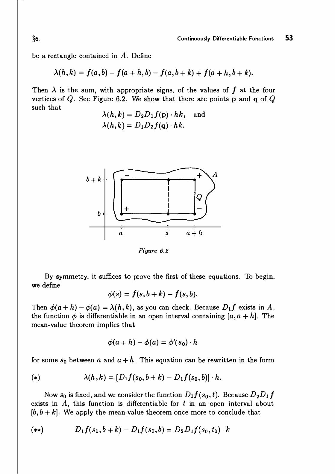
§6. Continuously Differentiable Functions 53
be a rectangle contained in A. Define
A ( h , k) = f (a , b) - f (a + h, b) - f (a , b + k) + f (a + h , b + k) .
Then A is the sum, with appropriate signs, of the values of f at the four vertices of Q. See Figure 6.2. We show that there are points p and q of Q such that
b
A(h, k) = D2Dtf(p) · hk , and
A(h, k ) = D1D2/(q) · hk.
+
a
r I I
l s
Figure 6.2
By symmetry, it suffices to prove the first of these equations. To begin, we define
</>(s) = f(s, b + k) - f(s, b). Then </>(a + h) - </>(a) = A(h, k) , as you can check . Because Dd exists in A , the function </> is differentiable in an open interval containing [a , a + h] . The mean-value theorem implies that
</>(a + h) - </>(a) = </>' ( s0) · h
for some s0 between a and a + h. This equation can be rewritten in the form
A(h , k) = [Dd(so, b + k) - Dd(so , b)] · h .
Now s0 is fixed, and we consider the function Dd(s0 , t) . Because D2D1 f exists in A, this function is differentiable for t in an open interval about [b, b + k] . We apply the mean-value theorem once more to conclude that

54 Differentiation Chapter 2
for some t0 between b and b + k . Combining (*) and (**) gives our desired result .
Step 2. We prove the theorem. Given the point a = (a , b) of A and given t > 0, let Q1 be the rectangle
Qt = [a , a + t] x [b, b + t] .
If t is sufficiently small , Q 1 is contained in A; then Step 1 implies that
for some point Pt in Q 1 • If we let t - 0, then Pt - a. Because D2D1 f is continuous, it follows that
A similar argument , using the other equation from Step 1 , implies that
>.(t , t)ft2 - D1Dd(a) as t - 0.
The theorem follows. 0
EXERCISES
1 . Show that the function f(x, y) = lxyl is differentiable at 0, but is not of class C1 in any neighborhood of 0.
2. Define f : R --+ R by setting /(0) = 0, and
f(t) = e sin(l/t) if t f. 0 .
(a) Show f is differentiable at 0 , and calculate /'(0) .
(b) Calculate f' ( t) if t f. 0.
(c) Show f' is not continuous at 0.
(d) Conclude that f is differentiable on R but not of class C1 on R.
3 . Show that the proof of Theorem 6.2 goes through if we assume merely that the partials D1 f exist in a neighborhood of a and are continuous at a.
4. Show that if A C Rm and f : A --+ R, and if the partials D1f exist and are bounded in a neighborhood of a, then f is continuous at a.
5. Let f : R2 --+ R2 be defined by the equation
f(r, 9) = (r cos 9, r sin 9) .
It is called the polai' com·dinate transformation.

§6. Continuously Differentiable Functions
(a) Calculate D f and det D f. (b) Sketch the image under f of the set S = [1 , 2] x (0 , 1r] . [Hint: Find
the images under f of the line segments that bound S .] 6. Repeat Exercise 5 for the function f : R2 --+ R2 given by
Take S to be the set
[Hint: Parametrize part of the boundary of S by setting x = a cos t and y = a sin t ; find the image of this curve. Proceed similarly for the rest of the boundary of S.]
We remark that if one identifies the complex numbers C with R2 in the usual way, then f is just the function f(z) = z2 •
7. Repeat Exercise 5 for the function f : R2 --+ R2 given by
f(x, y) = (ex cos y, ex sin y) .
Take S to be the set S = (0, 1] x (0, 1r] . We remark that if one identifies C with R2 as usual, then f is the
function f(z) = ez. 8. Repeat Exercise 5 for the function f : R3 --+ R3 given by
f(p, ¢>, 0) = (pcos O sin ¢, p sin O sin ¢, p cos ¢) .
It is called the spherical com·dinate transformation. Take S to be the set
S = (1 , 2] X (0, 1r /2] X (0 , 1r /2] .
9 . Let g : R --+ R be a function of class C2 . Show that
I . g(a + h) - 2g(a) + g(a - h) _ "( ) 1m h2 - g a .
h-o
[Hint: Consider Step 1 of Theorem 6 .3 in the case f(x, y) = g(x + y).] *10. Define f : R2 --+ R by setting /(0) = 0, and
f(x ,y) = xy(x2 - y2 )/(x2 + y2 ) if (x , y) ,t: O.
(a) Show Dd and Dd exist at 0. (b) Calculate DI J and D2f at (x , y) # 0. (c) Show f is of class C1 on R2 • [Hint: Show Di f(x, y) equals the prod
uct of y and a bounded function, and D2/(x, y) equals the product of X and a bounded function.]
(d) Show that D2DI/ and D1 D2/ exist at O, but are not equal there.
55

56 Differentiation Chapter 2
§7. THE CHAIN R U L E
In this section we show that the composite of two differentiable functions is differentiable, and we derive a formula for its derivative. This formula is commonly called the "chain rule."
Theorem 7 . 1 . Let A c Rm ; let B c Rn . Let
f : A --+ Rn and g : B --+ RP,
with f (A) C B . Suppose f (a) = b. If f is differentiable at a, and if g is differentiable at b, then the composite function g o f is differentiable at a. Furthermore,
D(g o /)(a) = Dg(b) · Df(a) ,
where the indicated product is matrix multiplication.
Although this version of the chain rule may look a bit strange, it is really just the familiar chain rule of calculus in a new guise. You can convince yourself of this fact by writing the formula out in terms of partial derivatives. We shall return to this matter later.
Proof. For convenience , let x denote the general point of Rm , and let y denote the general point of Rn.
By hypothesis, g is defined in a neighborhood of b; choose E so that g(y) is defined for IY - bl < E. Similarly, since f is defined in a neighborhood of a and is continuous at a, we can choose b so that f(x) is defined and satisfies the condition l f(x) - bl < E, for lx - al < b. Then the composite function (g o f)(x) = g(/(x)) is defined for l x - al < b. See Figure 7 . 1 .
I 6 1
. a f
Figure 7.1
g • c
z E RP

§7.
Step 1 . Throughout, let 6-(h) denote the function
6-(h) = /(a + h) - /(a) ,
The Chain Rule 57
which is defined for [h i < b. First, we show that the quotient [6-(h) l /lhl is bounded for h in some deleted neighborhood of 0.
For this purpose, let us introduce the function F(h) defined by setting F(O) = 0 and
F(h) = [6-(h) -��/(a) · h) for 0 < [hi < b.
Because f is differentiable at a, the function F is continuous at 0. Furthermore, one has the equation
6-(h) = D f(a) · h + [h [F(h)
for 0 < [h[ < b, and also for h = 0 (trivially) . The triangle inequality implies that
[6-(h) l < m[DJ(a) [ lh l + [h[ [F(h) [ . Now [F(h) l is bounded for h in a neighborhood of 0; in fact, it approaches 0 as h approaches 0. Therefore [6-(h) l / [h i is bounded on a deleted neighborhood of 0.
Step 2. We repeat the construct ion of Step 1 for the function g. We define a function G(k) by setting G(O) = 0 and
G(k) = g(b + k) - g(b) - Dg(b) . k
lkl for 0 < [kl < E.
Because g is differentiable at b, the function G is continuous at 0. Furthermore, for [kl < E, G satisfies the equation
g(b + k) - g(b) = Dg(b) · k + [k [G(k) .
Step 3. We prove the theorem. Let h be any point of Rm with [h [ < b. Then [6-(h) [ < E, so we may substitute 6-(h) for k in formula ( * * ) . After this substitution, b + k becomes
b + 6-(h) = /(a) + 6-(h) = /(a + h),
so formula ( * *) takes the form
g(f(a + h)) - g(f(a)) = Dg(b) · 6-(h) + [6.(h) IG(6.(h)) .

58 Differentiation Chapter 2
Now we use ( * ) to rewrite this equation in the form
1 ThT [g (f(a + h)) - g (f(a)) - Dg(b) . D f(a) . h] 1 = Dg(b) · F(h) + ThT I �(h) IG(�(h)) .
This equation holds for 0 < I h i < b. In order to show that go f is differentiable at a with derivative Dg(b) · Df(a) , it suffices to show that the r ight side of this equation goes to zero as h approaches 0.
The matrix Dg(b) is constant, while F(h) -+ 0 as h -+ 0 (because F is continuous at 0 and vanishes there) . The factor G(�(h)) also approaches zero as h -+ 0; for it is the composite of two functions G and �. both of which are continuous at 0 and vanish there. Finally, l�(h) l / lhl is bounded in a deleted neighborhood of 0, by Step 1 . The theorem follows. 0
Here is an immediate consequence:
Corollary 7.2. Let A be open in Rm; let B be open in Rn . Let
f : A -+ Rn and g : B -+ RP ,
with f(A) c B . Iff and g are of class cr , so is the composite function g 0 f.
Proof. The chain rule gives us the formula
D(g o f)(x) = Dg(f(x)) · D f(x) ,
which holds for x E A. Suppose first that f and g are of class C1 • Then the entries of Dg are
continuous real-valued functions defined on B; because f is continuous on A, the composite function Dg (f(x)) is also continuous on A. Similarly, the entries of the matrix D f(x) are continuous on A. Because the entries of the matrix product are algebraic functions of the entries of the matrices involved, the entries of the product Dg (f(x)) · D f(x) are also continuous on A. Then g o f is of class C1 on A.
To prove the general case, we proceed by induction. Suppose the theorem is true for functions of class cr- 1 . Let f and g be of class Cr . Then the entries of Dg are real-valued functions of class cr- 1 on B. Now f is of class cr- 1 on A (being in fact of class cr ) ; hence the induction hypothesis implies that the function Digi (f(x)) , which is a composite of two functions of class cr- I ' is of class cr- I . Since the entries of the matrix D f (X) are also of class cr-1 on A by hypothesis , the entries of the product Dg (f(x)) · D f(x) are of class cr- l on A. Hence g o J is of class Cr on A, as desired .

§7. The Chain Rule
The theorem follows for r finite. If now f and g are of class coo, then they are of class cr for every r, whence g 0 f is also of class cr for every r. 0
As another application of the chain rule, we generalize the mean-value theorem of single-variable analysis to real-valued functions defined in Rm . We will use this theorem in the next section.
Theorem 7.3 (Mean-value theorem). Let A be open in Rm ; let f : A -+ R be differentiable on A . If A contains the line segment with end points a and a+ h, then there is a point c = a + t0h with 0 < t0 < 1 of this line segment such that
f(a + h) - /(a) = Df(c) · h.
Proof. Set ¢>(t) = /(a + th) ; then ¢> is defined for t in an open interval about [0, 1] . Being the composite of differentiable functions, ¢> is differentiable; its derivative is given by the formula
¢>'(t) = D f(a + th) · h.
The ordinary mean-value theorem implies that
¢(1) - ¢>(0) = ¢>' (to) · 1
for some to with 0 < t0 < 1 . This equation can be rewritten in the form
/(a + h) - /(a) = D f(a + toh) · h. 0
As yet another application of the chain rule, we consider the problem of differentiating an inverse function.
Recall the situation that occurs in single-variable analysis. Suppose ¢>(x) is differentiable on an open interval, with ¢>' (x) > 0 on that interval. Then ¢> is strictly increasing and has an inverse function '1/J, which is defined by letting '1/J(y) be that unique number x such that ¢>(x) = y. The function '1/J is in fact differentiable, and its derivative satisfies the equation
'1/J' (y) = 1/c/>'(x) ,
where y = ¢>(x) . There is a similar formula for differentiating the inverse of a function f
of several variables. In the present section, we do not consider the question whether the function f has an inverse, or whether that inverse is d ifferentiable. We consider only the problem of finding the derivative of the inverse function.
59
60 Differentiation Chapter 2
Theorem 7.4. Let A be open in Rn; let f : A -+ Rn ; let f(a) = b. Suppose that g maps a neighborhood of b into Rn , that g(b) = a, and
g(f(x)) = x
for all x in a neighborhood of a. If f is differentiable at a and if g is differentiable at b, then
Dg(b) = [D f(a)]- 1 •
Proof. Let i : Rn -+ Rn be the identity function; its derivative is the identity matrix In . We are given that
g (f(x)) = i(x)
for all x in a neighborhood of a. The chain rule impl ies that
Dg(b) · Df(a) = In .
Thus Dg(b) is the inverse matrix to Df(a) (see Theorem 2 .5) . 0
The preceding theorem implies that if a differentiable function f is to have a differentiable inverse , it is necessary that the matrix D f be non-singular . It is a somewhat surprising fact that this condition is also sufficient for a function f of class C1 to have an inverse , at least locally. We shall prove this fact in the next section .
REMARK. Let us make a comment on notation. The usefulness of well-chosen notation can hardly be overemphasized. Arguments that are obscure, and formulas that are complicated, sometimes become beautifully simple once the proper notation is chosen. Our use of matrix notation for the derivative is a case in point . The formulas for the derivatives of a composite function and an inverse function could hardly be simpler.
Nevertheless, a word may be in order for those who remember the notation used in calculus for partial derivatives, and the version of the chain rule proved there.
In advanced mathematics, it is usual to use either the functional notation ¢' or the operator notation D¢> for the derivative of a real-valued function of a real variable. ( D¢> denotes a 1 by 1 matrix in this case!) In calculus, however, another notation is common. One often denotes the derivative ¢'(x) by the symbol d¢>/dx, or, introducing the "variable" y by setting y = ¢>(x), by the symbol dyjdx . This notation was introduced by Leibnitz, one of the originators of calculus. It comes from the time when the focus of every physical and mathematical problem was on the varia bles involved, and when functions as such were hardly even thought about.

§7. The Chain Rule
The Leibnitz notation has some familiar virtues. For one thing, it makes the chain rule easy to remember. Given functions ¢> : R --+ R and t/J : R --+ R, the derivative of the composite function t/J o ¢> is given by the formula
D(ljJ o ¢)(x) = Dt/J (¢>(x)) . D¢>(x) .
If we introduce variables by setting y = ¢>(x) and z = t/J(y), then the derivative of the composite function z = t/J (cf>(x)) can be expressed in the Leibnitz notation by the formula
dz dz dy dx = dy · dx ·
The latter formula is easy to remember because it looks like the formula for multiplying fractions! However, this notation has its ambiguities. The letter "z," when it appears on the left side of this equation, denotes one function (a function of x); and when it appears on the right side, it denotes a different function (a function of y). This can lead to difficulties when it comes to computing higher derivatives unless one is very careful.
The formula for the derivative of an inverse function is also easy to remember. If y = ¢>(x) has the inverse function X = 1/J(y), then the derivative of t/J is expressed in Leibnitz notation by the equation
1 dxfdy = dyfdx '
which looks like the formula for the reciprocal of a fraction! The Leibnitz notation can easily be extended to functions of several vari
ables. If A C Rm and f : A --+ R, we often set
Y = f(x) = f(xl , . . . , Xm) ,
and denote the partial derivative D;f by one of the symbols
of OX; or
The Leibnitz notation is not nearly as convenient in this situation. Consider the chain rule, for example. If
then the composite function F = g o f maps Rm into R, and its derivative is given by the formula
DF(x) = Dg (/(x)) · Df(x),
61

62 Differentiation Chapter 2
which can be written out in the form
DmF(x)]
Dng(/(x))]
The formula for the ph partial derivative of F is thus given by the equation
n DiF(x) = L Dkg(/(x)) Difk(x) .
k=l If we shift to "variable" notation by setting y = f(x) and z - g(y) , this equation becomes
this is probably the version of the chain rule you learned in calculus. Only familiarity would suggest that it is easier to remember than ( * ) ! Certainly one cannot obtain the formula for 8zj{)xi by a simple-minded multiplication of fractions, as in the single-variable case.
The formula for the derivative of an inverse function is even more troublesome. Suppose f : R2 _. R2 is differentiable and has a differentiable inverse function g. The derivative of g is given by the formula
Dg(y) = (Df(x)r1 .
where y = f(x). In Leibnitz notation, this formula takes the form
{)xi /8y2 ] = [8yd8x1
{)x2/ {)y2 8y2/ {)xi 8yt f {) x2 ] - l
{)y2/ 8x2
Recalling the formula for the inverse of a matrix, we see that the partial derivative {)x; / {)yi is about as far from being the reciprocal of the partial derivative 8yif {)x; as one could imagine!

§8. The Inverse Function Theorem
EXERCISES 1 . Let f : R3 --+ R2 satisfy the conditions /(0) = ( 1 , 2) and [ 1 2 3 ] D/ (0) = .
0 0 1 Let g : R2 --+ R2 be defined by the equation
g(x, y) = (x + 2y + 1 , 3xy) .
Find D(g o /)(0). 2. Let f : R2 --+ R3 and g : R3 --+ R2 be given by the equations
f(x) = (e2"' 1 +"'2 , 3X2 - COS X! , X� + X2 + 2) ,
g(y) = (3y1 + 2y2 + YL y� - Y3 + 1 ) . (a) If F(x) = g(/(x)) , find DF(O) . [Hint: Don't compute F explici tly.]
(b) If G(y) = / (g(y)) , find DG(O) . 3. Let f : R3 --+ R and g : R2 --+ R be differentiable. Let F : R2 --+ R be
defined by the equation
F(x, y) = f(x, y, g(x, y)) .
(a) Find D F in terms of the partials of f and g. (b) If F(x , y) = 0 for all (x, y) , find D1g and D2g in terms of the partials
of f. 4. Let g : R2 --+ R2 be defined by the equation g( x, y) = ( x, y + x2 ) . Let
f : R2 --+ R be the function defined in Example 3 of § 5. Let h = f o g. Show that the directional derivatives of f and g exist everywhere, but that there is a u :j:. 0 for which h'(O; u) does not exist.
63
§8. T H E I NVERSE FUNCTION THEOREM
Let A be open in Rn ; let f : A -+ Rn be of class C1 . We know that for f to have a differentiable inverse, it is necessary that the derivative D f (x) of f be non-singular. We now prove that this condition is also sufficient for f to have a differentiable inverse, at least locally. This result is called the inverse function theorem.
We begin by showing that non-singularity of D f implies that f is locally one-to-one.

64 Differentiation Chapter 2
Lemma 8.1 . Let A be open in Rn ; let f : A -+ Rn be of class C1 • If D f(a) is non-singular, then there exists an a > 0 such that the inequality
1 /(xo) - /(xi ) I > alxo - xd
holds for all x0 ,x1 in some open cube C(a; E) centered at a. It follows that f is one-to-one on this open cube.
Proof. Let E = D f(a) ; then E is non-singular . We first consider the linear transformation that maps x to E · x. We compute
lxo - xd = IE-1 · (E · xo - E · xi ) I < n 1E- 1 1 · 1E · xo - E · xd .
If we set 2a = 1/n iE- 1 1 , then for all x0 , x1 in Rn ,
IE · xo - E · xd > 2alxo - xd .
Now we prove the lemma. Consider the function
H(x) = /(x) - E · x.
Then DH(x) = D f(x) -E, so that DH (a) = 0. Because H is of class C1 , we can choose E > 0 so that IDH(x) l < afn for x in the open cube C = C(a; E) . The mean-value theorem, applied to the ith component function of H, tells us that , given x0 ,x1 E C, there is a c E C such that
Then for xo ,xl E C, we have
alxo - xd > I H(xo ) - H(x1 ) l
The lemma follows. 0
= I f ( xo ) - E · xo - f ( x 1 ) + E · x d > IE · x1 - E · xo l - 1/(xl ) - /(xo) l > 2alxl - xol - 1/(xl ) - /(xo ) l .
Now we show that non-singularity of D f, in the case where f is one-toone, implies that the inverse function is differentiable.

§8. The Inverse Function Theorem 65
Theorem 8.2. Let A be open in Rn; let f : A -+ Rn be of class cr ; let B = /(A). Iff is one-to-one on A and if D f(x) is non-singular for x E A, then the set B is open in Rn and the inverse function g : B -+ A is of class cr .
Proof. Step 1 . We prove the following elementary result : If ¢> : A -+ R is differentiable and if ¢> has a local minimum at x0 E A, then D¢>(x0) = 0.
To say that ¢> has a local minimum at x0 means that ¢>(x) > ¢>(x0) for all x in a neighborhood of x0 . Then given u :f; 0,
¢>(x0 + tu) - ¢>(x0) > 0
for all sufficiently small values of t. Therefore
¢>'(xo ; u) = lim [¢>(xo + tu) - ¢>(xo)]ft t--+0
is non-negative if t approaches 0 through positive values, and is non-positive if t approaches 0 through negative values . It follows that ¢>' (x0 ; u) = 0. In particular, Dj ¢>(x0) = 0 for all j, so that D¢>(x0) = 0.
Step 2. We show that the set B is open in Rn . Given b E B, we show B contains some open ball B(b; t5) about b.
We begin by choosing a rectangle Q lying in A whose interior contains the point a = J- 1 (b) of A . The set Bd Q is compact , being closed and bounded in Rn . Then the set /(Bd Q) is also compact, and thus is closed and bounded in Rn . Because f is one-to-one, /(Bd Q) is disjoint from b; because /(Bd Q) is closed , we can choose t5 > 0 so that the ball B(b; 2t5) is disjoint from /(Bd Q) . Given c E B(b; t5) we show that c = f(x) for some x E Q; it then follows that the set /(A) = B contains each point of B(b; t5), as desired . See Figure 8 . 1 .
e x • a f
Q
/(Bd Q)
Figure 8.1

66 Differentiation Chapter 2
Given c E B(b; t5) , consider the real-valued function
¢>(x) = 1 1 /(x) - cll 2 ,
which is of class Cr . Because Q is compact , this function has a minimum value on Q; suppose that this minimum value occurs at the point x of Q. We show that /(x) = c.
Now the value of ¢> at the point a is
¢>(a) = 1 1 /(a) - cl l2 = l ib - cll 2 < t52 •
Hence the minimum value of ¢> on Q must be less than t52 • It follows that this minimum value cannot occur on Bd Q, for if x E Bd Q , the point /(x) lies outside the ball B(b ; 2t5), so that 1 1 /(x) - el l > t5. Thus the minimum value of ¢> occurs at a point x of Int Q .
Because x is interior to Q , it follows that ¢> has a local minimum at x; then by Step 1 , the derivative of ¢> vanishes at x. Since
n
n Dj c/>(x) = L 2(f,, (x) - c�c)Di f�c (x) .
k=l
The equation D¢>(x) = 0 can be written in matrix form as
2[(ft(x) - cl ) Un (x) - Cn)] · D /(x) = 0.
Now Df(x) is non-singular , by hypothesis. Multiplying both sides of this equation on the right by the inverse of D f(x), we see that f(x) - c = O , as desired.
Step 3. The function f : A --+ B is one-to-one by hypothesis; let g : B --+ A be the inverse function. We show g is continuous.
Continuity of g is equivalent to the statement that for each open set U of A, the set V = g- 1 (U) is open in B. But V = f(U); and Step 2 , applied to the set U, which is open in A and hence open in Rn , tells us that V is open in Rn and hence open in B. See Figure 8 .2.

§8. The Inverse Function Theorem
f
g
Figure 8.2
It is an interesting fact that the results of Steps 2 and 3 hold without assuming that D f ( x) is non-singular, or even that f is differentiable. If A is open in R" and f : A --+ R" is continuous and one-to-one, then it is true that f(A) is open in R" and the inverse function g is continuous. This result is known as the Brouwer theorem on in variance of domain. Its proof requires the tools of algebraic topology and is quite difficult. We have proved the differentiable version of this theorem.
Step 4. Given b E B, we show that g is differentiable at b. Let a be the point g(b ) , and let E = D f(a) . We show that the function
G(k) = [g(b + k) - g(b) - E- 1 . k]
lkl '
which is defined for k in a deleted neighborhood of 0, approaches 0 as k approaches 0. Then g is differentiable at b with derivative E- 1 .
Let us define �(k) = g(b + k) - g(b)
for k near 0. We first show that there is an E > 0 such that l�(k) l/ lkl is bounded for 0 < lk l < E. (This would follow from differentiability of g, but that is what we are trying to prove!) By the preced ing lemma, there IS a neighborhood C of a and an a > 0 such that
l f(xo ) - f(x! ) l > alxo - xd for x0 , x1 E C . Now f(C) is a neighborhood of b , by Step 2 ; choose E so that h+k is in /(C) whenever lk l < E. Then for lk l < E, we can set x0 = g(b + k) and x1 = g(b) and rewrite the preceding inequality in the form
l (b + k) - bl > alg(b + k) - g(b) l ,
67

68 Differentiation Chapter 2
which implies that 1/a > l�(k) l / lk l ,
as desired. Now we show that G(k) -+ 0 as k -+ 0. Let 0 < lk l < E. We have
G(k) = �(k) jkf- 1 . k by definition ,
= -E-1 . [k - E · �(k) ] l�(k) l l�(k) l lkl .
(Here we use the fact that �(k) :f; 0 for k :f; 0 , which follows from the fact that g is one-to-one. ) Now E- 1 is constant, and l�(k) l / lkl is bounded . It remains to show that the expression in brackets goes to zero. We have
b + k = f (g(b + k)) = f(g(b) + �(k)) = f(a + �(k)) . Thus the expression in brackets equals
f (a + �(k)) - /(a) - E · �(k) l�(k) l
Let k -+ 0 . Then �(k) -+ 0 as well, because g is continuous. Since f is differentiable at a with derivative E, this expression goes to zero, as desired .
Step 5. Finally, we show the inverse function g is of class cr . Because g is differentiable, Theorem 7 .4 applies to show that its derivative
is given by the formula Dg(y) = [D / (g(y))] - 1 ,
for y E B . The function Dg thus equals the composite of three functions:
B .-!..... A .!!.!... GL(n) _!__. GL(n), where G L( n) is the set of non-singular n by n matrices, and I is the function that maps each non-singular matrix to its inverse. Now the function I is given by a specific formula involving determinants. In fact, the entries of /(C) are rational functions of the entries of C; as such , they are coo functions of the entries of C.
We proceed by induction on r. Suppose f is of class C1 • Then D f is continuous. Because g and I are also continuous (indeed , g is differentiable and I is of class C00) , the composite function, which equals Dg, is also continuous. Hence g is of class C1 •
Suppose the theorem holds for functions of class cr- 1• Let f be of class Cr. Then in particular f is of class cr-1 , so that (by the induction hypothesis) , the inverse function g is of class cr- 1 • Furthermore, the function D f is of class cr- 1 • We invoke Corollary 7.2 to conclude that the composite function , which equals Dg, is of class cr- 1 • Then g is of class cr . 0
Finally, we prove the inverse function theorem.

§8. The Inverse Function Theorem
Theorem 8.3 (The inverse function theorem) . Let A be open in Rn; let f : A -+ Rn be of class cr . If Df(x) is non-singular at the point a of A, there is a neighborhood U of the point a such that f carries U in a one-to-one fashion onto an open set V of Rn and the inverse function is of class cr .
Proof. By Lemma 8 . 1 , there is a neighborhood U0 of a on which f is one-to-one. Because det D f(x) is a continuous function ofx, and det D f(a) :f; 0, there is a neighborhood U1 of a such that det D f(x) :f; 0 on U1 • If U equals the intersection of Uo and U1 , then the hypotheses of the preceding theorem are satisfied for f : U -+ Rn . The theorem follows. 0
This theorem is the strongest one that can be proved in general . While the non-singularity of D f on A implies that f is locally one-to-one at each point of A, it does not imply that f is one-to-one on all of A. Consider the following example:
EXAMPLE 1. Let f : R2 --+ R2 be defined by the equation
Then
f ( r, 0) = ( r cos (} , r sin 0) .
[ cos O -rsin O] Df(r, O) = ,
sin (} r cos (} so that det D f( r, 0) = r.
Let A be the open set (0, 1 ) x (O , b) in the (r, O) plane. Then Df is nonsingular at each point of A. However, f is one-to-one on A only if b < 27r. See Figures 8.3 and 8.4.
(} 27r
f y
1
Figure 8.3
69

70 Differentiation Chapter 2
(J 27r
f y
1
Figure 8.4
EXERCISES
1 . Let f : R2 --+ R2 be defined by the equation
f(x , y) = (x2 - � , 2xy) .
(a) Show that f is one-to-one on the set A consisting of all (x, y) with x > 0. [Hint: If f(x, y) = f(a , b) , then 1 1/(x , y) ll = 1 1/(a , b) l l ·l
(b) What is the set B = f(A)?
(c) If g is the inverse function, find Dg(O, 1) . 2 . Let f : R2 --+ R2 be defined by the equation
f(x, y) = (ex cos y, ex sin y) .
(a) Show that f is one-to-one on the set A consisting of all (x, y) with 0 < y < 27r. (Hint: See the hint in the preceding exercise.]
(b) What is the set B = f(A)?
(c) If g is the inverse function , find Dg(O, 1 ) . 3 . Let f : Rn --+ Rn be given by the equation f(x) = llxll 2 · x. Show that
f is of class Coo and that f carries the unit ball B(O; 1) onto itself in a one-to-one fashion. Show, however , that the inverse function is not differentiable at 0.
4. Let g : R2 --+ R2 be given by the equation
Let f : R2 --+ R3 be given by the equation

§9. The Implicit Function Theorem
(a) Show that there is a neighborhood of (0, 1 ) that g carries in a oneto-one fashion onto a neighborhood of (2 , 0) .
(b) Find D(f o g-1 ) at (2, 0). 5. Let A be open in Rn; let f : A --+ Rn be of class C" ; assume Df(x) is
non-singular for X E A. Show that even if f is not one-to-one on A, the set B = f(A) is open in Rn.
71
*§9. THE I M PLICIT FU NCTION THEOREM
The topic of implicit differentiation is one that is probably familiar to you from calculus. Here is a typical problem:
"Assume that the equation x3y + 2exy = 0 determines y as a differentiable function of x . Find dyldx."
One solves this calculus problem by "looking at y as a function of X ," and differentiating with respect to x . One obtains the equation
which one solves for dy / dx . The derivative dy I dx is of course expressed in terms of X and the unknown function y.
The case of an arbitrary function f is handled similarly. Supposing that the equation f(x , y) = 0 determines y as a differentiable function of x, say y = g(x) , the equation f (x , g(x)) = 0 is an identity. One applies the chain rule to calculate
so that
8/ l8x + (8/ 18y)g' (x) = 0,
, 8fl8x g (X) = - 8 f I 8y '
where the partial derivatives are evaluated at the point (x, g(x)) . Note that the solution involves a hypothesis not given in the statement of the problem. In order to find g'(x) , it is necessary to assume that 8/ l8y is non-�ero at the point in question.
It in fact turns out that the non-vanishing of 8 f I 8y is also sufficient to justify the assumptions we made in solving the problem. That is, if the function f(x , y) has the property that 8 f I 8y :f; 0 at a point (a , b) that is a solution of the equation f(x, y) = 0, then this equation does determine y as a function of x, for x near a , and this function of x is differentiable.
72 Differentiation Chapter 2
This result is a special case of a theorem called the implicit function theorem, which we prove in this section .
The general case of the implicit function theorem involves a system of equations rather than a single equation . One seeks to solve this system for some of the unknowns in terms of the others. Specifically, suppose that f : Rk+n -+ Rn is a function of class C1 • Then the vector equation
is equivalent to a system of n scalar equations in k + n unknowns. One would expect to be able to assign arbitrary values to k of the unknowns and to solve for the remaining unknowns in terms of these. One would also expect that the resulting functions would be differentiable, and that one could by implicit differentiation find their derivatives.
There are two separate problems here. The first is the problem of finding the derivatives of these implicitly defined functions, assuming they exist; the solution to this problem generalizes the computation of g' ( x) just given. The second involves showing that (under suitable conditions) the implicitly defined functions exist and are differentiable.
In order to state our results in a convenient form, we introduce a new notation for the matrix D f and its submatrices:
Definition. Let A be open in Rm ; let f : A -+ Rn be differentiable. Let /1 , . . . , fn be the component functions of f . We sometimes use the notation
for the derivative of f. On occasion we shorten this to the notation
Df = 8f/8x.
More generally, we shall use the notation
8(/; 1 ' . . . ' f;k ) 8(xiu . . . , xit )
to denote the k by f matrix that consists of the entries of D f lying in rows i 1 , • • • , ik and columns j1 , • • • , jl . The general entry of this matrix, in row p and column q , is the partial derivative 8J;. f8xiq ·
Now we deal with the problem of finding the derivative of an implicitly defined function, assuming it exists and is differentiable. For simplicity, we shall assume that we have solved a system of n equations in k + n unknowns for the last n unknowns in terms of the first k unknowns.
§9. The Implicit Function Theorem 73
Theorem 9.1. Let A be open in Rk+n ; let f : A -+ Rn be differentiable. Write f in the form f(x, y), for x E Rk and y E Rn ; then Df has the form
D f = [ 8 f I 8x 8 f I 8y] . Suppose there is a differentiable function g : B -+ Rn defined on an open set B in Rk, such that
f (x, g(x)) = 0
for all x E B. Then for x E B,
�� (x, g(x)) + �� (x, g(x)) · Dg(x) = 0.
This equation implies that if the n by n matrix 8 f I 8y is non-singular at the point (x, g(x)) , then
[8f ] -l 8f Dg(x) = - 8y (x, g(x)) · 8x (x, g(x)) .
Note that in the case n = k = 1 , this is the same formula for the derivative that was derived earlier; the matrices involved are 1 by 1 matrices in that case.
Proof. Given g, let us define h : B -+ Rk+n by the equation
h(x) = (x, g(x)) .
The hypotheses of the theorem imply that the composite function
H(x) = f(h(x)) = f (x, g(x)) is defined and equals zero for all x E B. The chain rule then implies that
as desired . 0
0 = DH(x) = D f (h(x)) · Dh(x)
= [�� (h(x)) �� (h(x))] · [n;(x) ] = �� (h(x)) + �� (h(x)) · Dg(x) ,
The preceding theorem tells us that in order to compute Dg, we must assume that the matrix 8 f I 8y is non-singular. Now we prove that the nonsingularity of 8 f I 8y suffices to guarantee that the function g exists and is differentiable.

7 4 Differentiation Chapter 2
Theorem 9.2 (Implicit function theorem) . Let A be open in Rk+n ; let f : A -+ Rn be of class Cr . Write f in the form f(x, y) , for x E Rk and y E Rn . Suppose that (a, b) is a point of A such that f(a, b) = 0 and
8f det
By(a, b) :f; 0.
Then there is a neighborhood B of a in Rk and a unzque continuous function g : B -+ Rn such that g(a) = b and
f (x,g(x)) = 0
for all X E B. The function g is in fact of class cr .
Proof. We construct a function F to which we can apply the inverse function theorem. Define F : A -+ Rk+n by the equation
F(x, y) = (x, f(x, y)) .
Then F maps the open set A of Rk+n into Rk x Rn = Rk+n . Furthermore,
DF = [ a/iax 8f�8J ·
Computing det DF by repeated application of Lemma 2.12, we have det DF = det 8f/8y . Thus DF is non-singular at the point (a, b) .
Now F(a, b) = (a, 0). Applying the inverse function theorem to the map F, we conclude that there exists an open set U x V of Rk+n about (a, b) (where U is open in Rk and V is open in Rn) such that:
( 1 ) F maps U x V in a one-to-one fashion onto an open set W in Rk+n containing (a, 0) .
(2) The inverse function G ; w -+ u X v is of class cr . Note that because F(x, y) = (x, f(x, y)) , we have
(x, y) = G(x, f(x, y)) .
Thus G preserves the first k coordinates, as F does . Then we can write G in the form
G(x, z) = (x, h(x, z))
for X E Rk and z E Rn; here h is a function of class cr mapping w into Rn. Let B be a connected neighborhood of a in Rk , chosen small enough that
B x 0 is contained in l¥. See Figure 9 . 1 . We prove existence of the function g : B -+ Rn . If x E B , then (x, O) E 1¥ , so we have:
G(x, 0) = (x, h(x, 0)) , (x, O) = F(x, h(x, O )) = (x, f(x, h(x, O)) ) ,
0 = f(x, h(x, o)) .

§9.
(x, g(x))
v --r(a, b)
u
F G
Figure 9. 1
The Implicit Function Theorem
( (x, O)
/(a, O)
B
w
We set g(x) = h(x, 0) for x E B; then g satisfies the equation f(x, g(x)) = 0 , as desired. Furthermore,
(a, b) = G(a, O) = (a, h(a, O)) ;
then b = g(a), as desired . Now we prove uniqueness of g. Let go : B - Rn be a continuous function
satisfying the conditions in the conclusion of our theorem. Then in particular, g0 agrees with g at the point a. We show that if g0 agrees with g at the point a0 E B, then g0 agrees with g in a neighborhood Bo of a0 • This is easy. The map g carries a0 into V. Since g0 is continuous, there is a neighborhood B0 of a0 contained in B such that g0 also maps B0 into V. The fact that f (x, go(x)) = 0 for x E Eo implies that
F(x, g0(x)) = (x, O) , so
(x, g0(x)) = G(x, O) = (x, h(x, O)) .
Thus go and g agree on B0• It follows that go and g agree on all of B: The set of points of B for which /g(x) - g0(x)/ = 0 is open in B (as we just proved) , and so is the set of points of B for which /g(x) - g0(x)/ > 0 (by continuity of g and g0) . Since B is connected, the latter set must be empty. 0
In our proof of the implicit function theorem, there was of course nothing special about solving for the last n coordinates ; that choice was made simply for convenience. The same argument applies to the problem of solving for any n coord inates in terms of the others.
75

7 6 Differentiation Chapter 2
For example, suppose A is open in R5 and f : A -+ R2 is a function of class cr . Suppose one wishes to "solve" the equation f(x, y, z , u, v) = o for the two unknowns y and u in terms of the other three. In this case, the implicit function theorem tells us that if a is a point of A such that /(a) = 0 and
det 8f
8(y, u) (a) :f; 0,
then one can solve for y and u locally near that point, say y = </>( x , z , v) and u = '1/J(x , z, v) . Furthermore, the derivatives of </> and '1/J satisfy the formula
8(</>, '1/J) [ 8! ] - l [ 8! ] 8(x , z, v)
= - 8(y, u) · 8(x , z, v) ·
EXAMPLE 1 . Let I : R2 --+ R be given by the equation
l(x, y) = x2 + lf - 5 .
Then the point (X , y) = ( 1 , 2) satisfies the equation l(x, y) = 0. Both {)I/ 8x and 81J8y are non-zero at (1 ,2), so we can solve this equation locally for either variable in terms of the other. In particular, we can solve for y in terms of x , obtaining the function
Note that this solution is not unique in a neighborhood of x = 1 unless we specify that g is continuous. For instance, the function
for x > 1 , for x < 1
satisfies the same conditions, but is not continuous. See Figure 9.2.
Y = g(x)
(1 , 2)
Figure 9.2
y = h(x)

§9. The Implicit Function Theorem
EXAMPLE 2. Let f be the function of Example 1 . The point (X, y) = ( VS, 0) also satisfies the equation f(x, y) = 0. The derivative {)jj{)y vanishes at ( VS, 0), so we do not expect to be able to solve for y in terms of X near this point. And, in fact, there is no neighborhood B of yS on which we can solve for y in terms of X . See Figure 9 .3 .
(VS, O)
Figure 9.3
EXAMPLE 3. Let f ; R2 --+ R be given by the equation
Then (0,0) is a solution of the equation f(x, y) = 0. Because {)j j{)y vanishes at (0,0), we do not expect to be able to solve this equation for y in terms of x near (0,0). But in fact, we can; and furthermore, the solution is unique! However, the function we obtain is not differentiable at x = 0. See Figure 9.4.
Figure 9.4
EXAMPLE 4. Let f ; R2 --+ R be given by the equation
Then (0,0) is a solution of the equation f(x, y) = 0. Because {)j J {)y vanishes at (0,0), we do not expect to be able to solve for y in terms of X near (0,0) . In
77

78 Differentiation Chapter 2
fact , however, we can do so, and we can do so in such a way that the resulting function is differentiable. However, the solution is not unique.
Figure 9.5
Now the point (1 ,2) also satisfies the equation f(x , y) = 0. Because of fay is non-zero at (1 ,2) , one can solve this equation for y as a continuous function of x in a neighborhood of x = 1 . See Figure 9.5. One can in fact express y as a continuous function of x on a larger neighborhood than the one pictured, but if the neighborhood is large enough that it contains 0, then the solution is not unique on that larger neighborhood.
EXERCISES
1 . Let f : R3 --+ R2 be of class C1 ; write f in the form f(x, YI , y2 ) . Assume that /(3, - 1 , 2 ) = 0 and
D/(3, -1 , 2) = [ 1
1
2
-1 � ] . (a) Show there is a function g : B --+ R2 of class C1 defined on an open
set B in R such that
I (X , YI (X) , Y2 (X)) = 0
for x E B, and g(3) = (-1 , 2).
(b) Find Dg(3). (c) Discuss the problem of solving the equation f(x , yl , Y2) = 0 for an
arbitrary pair of the unknowns in terms of the third, near the point (3, - 1 , 2) .
2 . Given f : R5 --+ R2 , of class C1 • Let a = (1 , 2 , -1 , 3 , 0) ; suppose that /(a) = 0 and
Df(a) = [ � : 1
1
-1
2

§9. The Implicit Function Theorem
(a) Show there is a function g : B --+ R2 of class C1 defined on an open set B of R3 such that
for x = (x 1 , X2 , X3) E B, and g( l , 3 , 0) = (2, -1) . (b) Find Dg( l , 3 , 0). (c) Discuss the problem of solving the equation f(x) = 0 for an arbitrary
pair of the unknowns in terms of the others, near the point a. 3. Let f : R2 --+ R be of class C1 , with /(2 , -1) = -1 . Set
G(x , y, u) = f(x, y) + u2 ,
H(x, y, u) = ux + 3y3 + u3 •
The equations G(x, y , u) = 0 and H(x , y, u) = 0 have the solution (x, y, u) = (2 , -1 , 1) . (a) What conditions on Df ensure that there are C1 functions X = g(y)
and u = h(y) defined on an open set in R that satisfy both equations, such that g(-1) = 2 and h(-1) = 1?
(b) Under the conditions of (a) , and assuming that D/(2 , -1) = [1 - 3] , find g' (-1) and h'(-1).
4. Let F : R2 ..... R be of class 02 , with F(O, 0) = 0 and DF(O, 0) = [2 3]. Let G : R3 --+ R be defined by the equation
G(x , y, z ) = F(x + 2y + 3z - 1 , x3 + y2 - z2 ) .
(a) Note that G(-2, 3 , -1) = F(O, O) = 0. Show that one can solve the equation G(x , y, z) = 0 for z, say z = g(x , y), for (x, y) in a neighborhood B of ( -2, 3), such that g( -2, 3) = -1 .
(b) Find Dg( -2, 3). *(c) If D1 D1F = 3 and D1 D2F = -1 and D2D2F = 5 at (0,0), find
D2D1g( -2, 3) . 5 . Let /, g : R3 --+ R be functions of class C1 • "In general," one expects
that each of the equations f(x, y, z ) = 0 and g(x , y, z) = 0 represents a smooth surface in R3 , and that their intersection is a smooth curve. Show that if (x0 , y0 , z0) satisfies both equations, and if 8(f, g)j8(x , y, z) has rank 2 at (xo , yo , zo) , then near (xo , yo , zo ) , one can solve these equations for two of x , y , z in terms of the third, thus representing the solution set locally as a parametrized curve.
6. Let f : Rk+n --+ Rn be of class C1 ; suppose that /(a) = 0 and that Df(a) has rank n . Show that if c is a point of Rn sufficiently close to 0, then the equation /(x) = c has a solution.
79


Integration
In this chapter, we define the integral of real-valued function of several real variables, and derive its properties. The integral we study is called Riemann integral ; it is a direct generalization of the integral usually studied in a first course in single-variable analysis.
§10 . THE INTEGRAL OVER A RECTANGLE
We begin by defining the volume of a rectangle. Let
be a rectangle in Rn . Each of the intervals [a;, b;] is called a component interval of Q. The maximum of the numbers b1 - a1 , . . . , bn - an is called the width of Q. Their product
is called the volume of Q. In the case n = 1 , the volume and the width of the (!-dimensional)
rectangle [a, b] are the same, namely, the number b - a. This number is also called the length of [a, b ] .
Definition. Given a closed interval [a, b] of R, a partition of [a, b] is a finite collection P of points of [a, b] that includes the points a and b . We
8 1

82 Integration Chapter 3
usually index the elements of P in increasing order, for notational convenience, as
a = to < t 1 < · · · < t�c = b; each of the intervals [ t; - 1 , t; ] , for i = 1 , . . . , k, is called a subinterval determined by P, of the interval [a , b] . More generally, given a rectangle
in Rn, a partition P of Q is an n-tuple ( P� , . . . , Pn ) such that P; is a partition of [a; , bi] for each j . If for each j, I; is one of the subintervals determined by Pi of the interval [ai , bi] , then the rectangle
R = I1 X · · · X In
is called a subrectangle determined by P, of the rectangle Q. The maximum width of these subrectangles is called the mesh of P.
Definition. Let Q be a rectangle in Rn ; let f : Q --+ R; assume f is bounded. Let P be a partition of Q. For each subrectangle R determined by P, let
mR(/) = inf{ f(x) I x E R} , MR(/) = sup{ f(x) I x E R} .
We define the lower sum and the upper sum, respectively, of f , determined by P, by the equations
L(f, P) = L mR(/) · v(R) , R
U(f, P) = L MR(/) · v(R) , R
where the summations extend over all subrectangles R determined by P.
Let P = ( P1 , . . . , Pn ) be a partition of the rectangle Q . If P" is a partition of Q obtained from P by adjoining additional points to some or all of the partitions P1 , • . . , Pn , then P" is called a refinement of P. Given two partitions P and P' = ( P{ , . . . , P�) of Q , the partition
P" = ( P1 U P{ , . . . , Pn U P�)
is a refinement of both P and P' ; it is called their common refinement. Passing from P to a refinement of P of course affects lower sums and
upper sums; in fact , it tends to increase the lower sums and decrease the upper sums. That is the substance of the following lemma:

§10. The Integral Over a Rectangle 83
Lemma 10.1. Let P be a partition of the rectangle Q; let f : Q -+ R be a bounded function. If P" is a refinement of P, then
L(f, P) < L(f, P") and U(f, P") < U(f, P).
Proof. Let Q be the rectangle
Q = [a 1 , b i] X · · · X [an, bn] ·
It suffices to prove the lemma when P" is obtained by adjoining a single additional point to the partition of one of the component intervals of Q . Suppose, to be definite, that P is the partition ( P1 , • • • , Pn ) and that P" is obtained by adjoining the point q to the partition P1 . Further, suppose that P1 consists of the points
and that q lies interior to the subinterval [ti- t , t;] . We first compare the lower sums L(f, P) and L(f, P"). Most of the
subrectangles determined by P are also subrectangles determined by P". An exception occurs for a subrectangle determined by P of the form
(where S is one of the subrectangles of [a2 , b2] x · · · x [an , bn] determined by (P2 , . . . , Pn)) . The term involving the subrectangle Rs disappears from the lower sum and is replaced by the terms involving the two subrectangles
R� = [ti -h q] x S and R� = [q, t;] x S,
which are determined by P". See Figure 10 . 1 .
,-R�/R� t Jf
s � � �V//.
I !
Q
q
Figure 1 0.1

84 Integration Chapter 3
Now since fiR5 (/) < /(x) for each x E R� and for each x E R� , it follows that
Because v(Rs) = v(R's) + v(R�) by direct computation , we have
Since this inequality holds for each subrectangle of the form Rs , it follows that
L(/, P) < L(/, P") , as desired .
A similar argument applies to show that U(/, P) > U(/, P") . 0
Now we explore the relation between upper sums and lower sums. We have the following result :
Lemma 10.2. Let Q be a rectangle; let f : Q -+ R be a bounded function. If P and P' are any two partitions of Q, then
L(/, P) < U(/, P' ) .
Proof. In the case where P = P' , the result is obvious: For any subrectangle R determined by P, we have mR(/) < MR(/). Multiplying by v(R) and summing gives the desired inequality.
In general, given partitions P and P' of Q, let P" be their common refinement. Using the preceding lemma, we conclude that
L(/, P) < L(/, P") < U(/, P") < U(f, P'). 0
Now (finally) we define the integral .
Definition. Let Q be a rectangle; let f : Q -+ R be a bounded function. As P ranges over all partitions of Q , define
r I = sup {L(f, P)} jg p and [ f = inf {U(f, P)} . JQ p
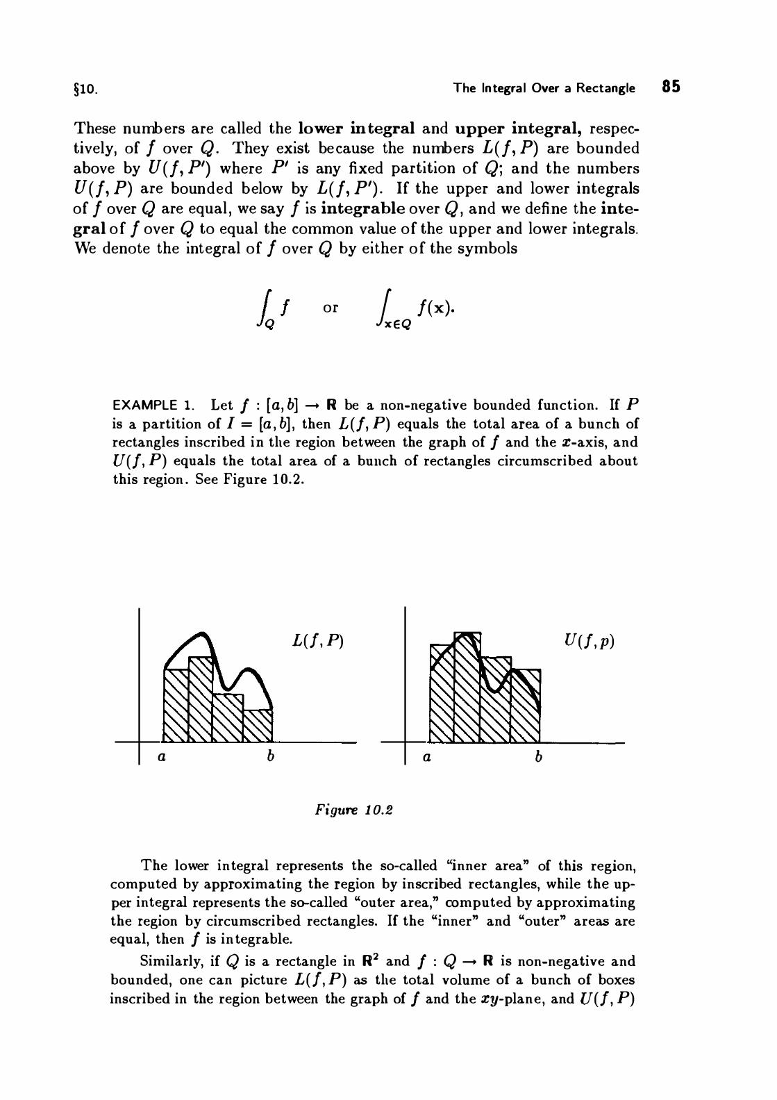
§10. The Integral Over a Rectangle
These numbers are called the lower integral and upper integral, respectively, of f over Q. They exist because the numbers L(f, P) are bounded above by U(f, P') where P' is any fixed partition of Q; and the numbers U(f, P) are bounded below by L(f, P') . If the upper and lower integrals of f over Q are equal , we say f is integrable over Q , and we define the integral of f over Q to equal the common value of the upper and lower integrals. We denote the integral of f over Q by either of the symbols
or 1 f(x). xEQ
EXAMPLE 1. Let I : (a, b] --+ R be a non-negative bounded function. If P is a partition of I = (a , b] , then L(/, P) equals the total area of a bunch of rectangles inscribed in the region between the graph of I and the X-axis, and U(f, P) equals the total area of a bunch of rectangles circumscribed about this region . See Figure 1 0.2.
L(f, P) U(f, p)
a b a b
Figure 1 0.2
The lower integral represents the so-called "inner area" of this region, computed by approximating the region by inscribed rectangles, while the upper integral represents the so-called "outer area," computed by approximating the region by circumscribed rectangles. If the "inner" and "outer" areas are equal, then I is integrable.
Similarly, if Q is a rectangle in R2 and I : Q --+ R is non-negative and bounded, one can picture L(f, P) as the total volume of a bunch of boxes inscribed in the region between the graph of I and the xy-plane, and U(f, P)
85

86 I ntegration Chapter 3
as the total volume of a bunch of boxes circumscribed about this region. See Figure 10 .3 .
Figure 10.3
EXAMPLE 2. Let I = (0, 1] . Let I : I --+ R be defined by setting l (x) = 0 if x is rational, and l(x) = 1 if x is irrational. We show that I is not integrable over I.
Let P be a partition of I. If R is any subinterval determined by P, then m R(/ ) = 0 and MR(/) = 1 , since R contains both rational and irrational numbers. Then
L (/, P) = L 0 · v(R) = 0 , R
and U(/, P) = L 1 · v(R) = 1 .
R
Since P is arbitrary, it follows that the lower integral of I over I equals 0, and the upper integral equals 1 . Thus I is not integrable over I.
A condition that is often useful for showing that a given function is integrable is the following:
Theorem 10.3 (The Riemann condition) . let f : Q -+ R be a bounded function. Then
Let Q be a rectangle;
equality holds if and only if given E > 0, there exists a corresponding partition P of Q for which
U (f, P) - L(f, P) < c

§10. The Integral Over a Rectangle 87
Proof. Let P' be a fixed partition of Q . It follows from the fact that L(/, P) < U (/, P') for every partition P of Q, that
� I < U(f, P' ).
Now we use the fact that P' is arbitrary to conclude that
Suppose now that the upper and lower integrals are equal . Choose a partition P so that L(/, P) is within E/2 of the integral JQ /, and a partition P' so that U(/, P') is within E/2 of the integral JQ f . Let P" be their common refinement. Since
L(/, P) < L(/, P") < � f < U(/, P") < U(/, P' ) ,
the lower and upper sums for f determined by P" are within E of each other . Conversely, suppose the upper and lower integrals are not equal. Let
Let P be any partition of Q . Then
L(f, P) < � I < � I < U(f, P) ;
hence the upper and lower sums for f determined by P are at least E apart. Thus the Riemann condition does not hold . 0
Here is an easy application of this theorem.
Theorem 10.4. Every constant function f(x) = c is integrable. Indeed, if Q is a rectangle and if P is a partition of Q, then
1 c = c · v(Q) = c L: v(R), Q R
where the summation extends over all subrectangles determined by P.

88 Integration Chapter 3
Proof. If R is a subrectangle determined by P, then mR(/) = c = MR(/) . It follows that
L(f, P) = c L v(R) = U(f, P), R
so the Riemann condition holds trivially. Thus JQ c exists ; since it lies between L(f, P) and U(f, P) , it must equal c "ER v(R) .
This result holds for any partition P. In particular, i f P is the trivial partition whose only subrectangle is Q itself,
� c = c · v(Q). 0
A corollary of this result, which we shall use in the next section, is the following:
Corollary 10.5. Let Q be a rectangle in Rn; let {Q� , . . . , Qk } be a finite collection of rectangles that covers Q. Then
k
v(Q ) < L v(Q; ) . i= 1
Proof. Choose a rectangle Q' containing all the rectangles Q 1 , • . . , Q 1c . Use the end points of the component intervals of the rectangles Q ,Q 1 , . . . , Q�c to define a partition P of Q'. Then each of the rectangles Q, Q 1 , . . • , Q 1c is a union of sub rectangles determined by P. See Figure 10 .4 .
'T --- +- -1 I I I
l - - -- -· -- - -
- -I
--
I
r-I I
- - -t -t-I I
I I I
I
I I � : : I I
I I - - -r-I '
I : _ _ .1 _ - -r- -
I _ I .,... I
� -I
j_ _. _ -I l 1---
I I I - , - +- - -r -I I I
Figure 10.4
Q

§to. The Integral Over a Rectangle
From the preceding theorem, we conclude that
v(Q) = L v(R), RC Q
where the summation extends over all sub rectangles contained in Q. Because each such subrectangle R is contained in at least one of the rectangles Q1 , . . . ,Q �c, we have
k L v(R) < L L v(R) .
RC Q i = l RC Q;
Again using Theorem 10 .4, we have
L v(R) = v(Q;) ; Rc Q,
the corollary follows. 0
A remark about notation. We shall often use a slightly different notation for the integral in the case n = 1 . In this case, Q is a closed interval [a , b] in R , and we often denote the integral of f over [a , b] by one of the symbols
instead of the symbol fra,b] f. Yet another notation is used in calculus for the one-d imensional integral .
There it is common to denote this integral by the expression
1b f(x ) dx ,
where the symbol "dx" has no independent meaning. We shall avoid this notation for the time being. In a later chapter, we shall give "dx" a meaning and shall introduce this notation.
The definition of the integral we have given is in fact due to Darboux. An equivalent formulation, due to Riemann , is given in Exercise 7. In practice, it has become standard to call this integral the Riemann integral, independent of which definition is used.
89

90 Integration Chapter 3
EXERCISES
1 . Let J, g : Q --+ R be bounded functions such that /(x) < g(x) for X E Q. - -Show that Jq f < Jq g and Jq f < Jq g.
2. Suppose f : Q --+ R is continuous. Show f is integrable over Q. [Hint: Use uniform continuity of f.]
3. Let (0, 1]2 = [0, 1] x [0, 1]. Let f : (0, If --+ R be defined by setting f(x, y) = 0 if y ¥- x, and f(x, y) = 1 if y = x. Show that f is integrable over [0, 1]2 •
4. We say f : [0, 1] --+ R is increasing if /(x i ) < f(x2 ) whenever X1 < X2 . If /, g : (0, 1] --+ R are increasing and non-negative, show that the function h(x, y) = f(x)g(y) is integrable over [0 , 1]2 •
5 . Let f : R --+ R be defined by setting f(x) = 1/ q if X = pf q, where p and q are positive integers with no common factor, and f(x) = 0 otherwise. Show f is integrable over (0, 1].
*6. Prove the following:
Theorem. Let f : Q --+ R be bounded. Then f is integrable over Q if and only if given E > 0, there is a 6 > 0 such that U(/, P) - L (/, P) < E fo r every partition P of mesh less than 6.
Proof. (a) Verify the "if" part of the theorem.
(b) Suppose 1/(x) l < M for x E Q. Let P be a partition of Q. Show that if P" is obtained by adjoining a single point to the partition of one of the component intervals of Q, then
o < L(f, P") - L(/, P) < 2M(mesh P) (width Qt-1 •
Derive a similar result for upper sums.
(c) Prove the "only if" part of tbe theorem: Suppose f is integrable over Q. Given E > 0, choose a partition P' such that U(/, P') L(f, P') < E/2. Let N be the number of partition points in P'; then let
6 = E/BM N (width Qt-1 .
Show that if P has mesh less than 6, then U(/, P) - L(/, P) < E. [Hint: The common refinement of P and P' is obtained by adjoining at most N points to P.]
7. Use Exercise 6 to prove the following:
Theorem. Let f : Q --+ R be bounded. Then the statement that f is integrable over Q, with Jq f = A, is equivalent to the statement that given E > 0, there is a 6 > 0 such that if P is any partition of mesh less than 6, and if, fo r each subrectangle R determined by P, XR is a point of R, then
I L f(xR)v(R) - AI < E. R

§u. Existence of the Integral 91
§11 . EX ISTENCE OF THE INTEGRAL
In this section, we derive a necessary and sufficient condition for the existence of the integral JQ f. It involves the notion of a "set of measure zero."
Definition. Let A be a subset of Rn . We say A has measure zero in Rn if for every E > 0, there is a covering Qh Q2, . . . of A by countably many rectangles such that
00
L v(Qi ) < L i=l
If this inequality holds, we often say that the total volume of the rectangles Ql , Q2, . . . is less than E.
We derive some properties of sets of measure zero.
Theorem 11.1 . (a) If B C A and A has measure zero in Rn, then so does B.
(b) Let A be the union of the countable collection of sets A1 , A2 , . . . . If each Ai has measure zero in Rn, so does A.
(c) A set A has measure zero in Rn if and only if for every E > 0, there is a countable covering of A by open rectangles Int Q 1 , Int Q2, . . . such that
00
L v(Qi ) < L i=l
(d) If Q is a rectangle in Rn , then Bd Q has measure zero in Rn but Q does not.
Proof. (a) is immediate. To prove (b), cover the set Ai by countably many rectangles
Qlj ' Q2j , Q3j , 0 0 0 of total volume less than Ej2i . Do this for each j. Then the collection of rectangles { Qij } is countable, it covers A, and it has total volume less than
00
L Ef2i = E. j=l
(c) If the open rectangles Int Qh Int Q2, • • • cover A, then so do the rectangles Q1 , Q2, . . . . Thus the given condition implies that A has measure zero. Conversely, suppose A has measure zero. Cover A by rectangles

92 Integration Chapter 3
Q� , Q�, . . . of total volume less than E/2. For each i, choose a rectangle Q; such that
Qi C Int Q; and v(Q;) < 2v(Qi) . (This we can do because v(Q) is a continuous function of the end points of the component intervals of Q. ) Then the open rectangles Int Q1 , Int Q2 , . . . cover A, and 2::: v( Qi ) < E.
(d) Let Q = [ah b1] X • • • X [an , bn] ·
The subset of Q consisting of those points x of Q for which X; = a; is called one of the ith faces of Q. The other ith face consists of those x for which X; = b; . Each face of Q has measure zero in Rn ; for instance, the face for which X; = a; can be covered by the single rectangle
[a 1 , b 1] X • • • X [a; , a; + 6] X • • • X [an , bn] ,
whose volume may be made as small as desired by taking b small. Now Bd Q is the union of the faces of Q, which are finite in number. Therefore Bd Q has measure zero in Rn .
Now we suppose Q has measure zero in Rn , and derive a contradiction . Set E = v(Q) . We can by (c) cover Q by open rectangles Int Q 1 , Int Q2, • • • with L:: v(Qi ) < E. Because Q is compact, we can cover Q by finitely many of these open sets, say Int Qh . . . , Int Q�c. But
k Lv(Qi ) < E, i=l
a result that contradicts Corollary 10.5. 0
EXAMPLE 1. ."'.llowing for a countably infinite collection of rectangles is an essential part of the definition of a set of measure zero. One would obtain a different notion if one allowed only finite collections. For instance, the set A of rational numbers in I = (0, 1] is a countable union of one-point sets, so that A has measure zero in R by (b) of the preceding theorem. But A cannot be covered by finitely many intervals of total length less than E if E < 1 . For suppose I1 , . . . h is a finite collection of intervals covering A. Then the set B which is their union is a finite union of closed sets and therefore closed. Since B contains all rationals in I, it contains all limit points of these rationals; that is, it contains all of I. But this implies that the intervals I1 , . . . Ik cover I, whence by Corollary 10.5,
k L v(I; ) > v(I) = 1 . i=l
Now we prove our main theorem.

§n. Existence of the Integral 93
Theorem 11. 2. Let Q be a rectangle in Rn; let f : Q --+ R be a bounded function. Let D be the set of points of Q at which f fails to be continuous. Then JQ f exists if and only if D has measure zero in Rn .
Proof. Choose M so that lf(x) l < M for x E Q. Step 1 . We prove the "if' part of the theorem. Assume D has measure
zero in Rn . We show that f is integrable over Q by showing that given E > 0, there is a partition P of Q for which U(f, P) - L(f, P) < E.
Given E, let c be the strange number
E1 = E/ (2M + 2v(Q)) .
First, we cover D by countably many open rectangles Int Q1 , Int Q2, . . . of total volume less than E1 , using (c) of the preceding theorem. Second, for each point a of Q not in D, we choose an open rectangle Int Q8 containing a such that
lf(x) - f(a) l < E1 for X E Qa n Q . (This we can do because f is continuous at a. ) Then the open sets Int Q; and Int Q8, for i = 1 , 2, . . . and for a E Q - D, cover all of Q. Since Q is compact, we can choose a finite subcollection
Int Qt , . . . , Int Q�c , lnt Q81 , • • • , Int Qat
that covers Q. (The open rectangles Int Q b . . . , Int Q 1c may not cover D, but that does not matter. )
Denote Q81 by Qj for convenience. Then the rectangles
cover Q, where the rectangles Q; satisfy the condition
00
(1) Lv(Q;) < c, i=l
and the rectangles Qj satisfy the condition
(2) l f(x) - f(y) I < 2E1 for x, y E Qj n Q.
Without change of notation, let us replace each rectangle Q; by its intersection with Q, and each rectangle Q'. by its intersection with Q. The new rectangles {Q; } and {Qj } still cover Q and satisfy conditions ( 1 ) and (2) .
Now let us use the end points of the component intervals of the rectangles Q1 , . . . , Q�c , Q�, . . . , Q� to define a partition P of Q. Then each of the

94 Integration Chapter 3
rectangles Q; and Qj is a union of subrectangles determined by P. We compute the upper and lower sums of f relative to P.
Figure 1 1 . 1
Divide the collection o f all subrectangles R determined by P into two disjoint sub collections n and n' ' so that each rectangle R E n lies in one of the rectangles Q;, and each rectangle R E R' lies in one of the rectangles Qj . See Figure 1 1 . 1 . We have
L (MR(f) - mR(f)) v(R) < 2M L v(R), and RE'R. RE'R
RE'R' RE'R' these inequalities follow from the fact that
1 /(x) - /(y) l < 2M for any two points x,y belonging to a rectangle R E n, and
1/(x) - /(y) l < 2E1 for any two points x,y belonging to a rectangle R E n'. Now
Thus
k k L v(R) < L L v(R) = Lv(Q;) < E1 , and RE'R i:l RCQ, i=l
L v(R) < L v(R) = v(Q). RE'R' RCQ
U(f, P) - L(f, P) < 2M E1 + 2E'v(Q) = E.
§11 . Existence of the Integral 95
Step 2. We now define what we mean by the "oscillation" of a function f at a point a of its domain, and relate it to continuity of f at a.
Given a E Q and given b > 0, let A6 denote the set of values of /(x) at points x within b of a. That is,
A6 = {f(x) I x E Q and lx - al < 6} .
Let M6 (f) = sup A6 , and let m6 (/) = inf A6. We define the oscillation of f at a by the equation
v(f; a) = inf [M6(/) - m6(/)] . 6>0
Then v(f; a) is non-negative; we show that f is continuous at a if and only if v(/; a) = 0.
If f is continuous at a, then, given E > 0 , we can choose b > 0 so that 1/(x) - /(a) l < E for all x E Q with lx - al < b. It follows that
M6(/) < /(a) + E and m6(/) > /(a) - L
Hence v(f; a) < 2E. Since E is arbitrary, v(f; a) = 0. Conversely, suppose v(f; a) = 0. Given E > 0, there is a b > 0 such that
Now if x E Q and lx - al < b,
Since /(a) also lies between m6 (/) and M6(/) , it follows that 1/(x) - /(a)l < E. Thus f is continuous at a.
Step 3. We prove the "only if' part of the theorem. Assume f is integrable over Q. We show that the set D of discontinuities of f has measure zero in Rn .
For each positive integer m, let
Dm = {a I v(/ ; a) > 1/m } .
Then by Step 2, D equals the union of the sets Dm . We show that each set Dm has measure zero; this will suffice .
Let m be fixed. Given E > 0 , we shall cover Dm by countably many rectangles of total volume less than E.
First choose a partition P of Q for which U(f, P) - L(f, P) < E/2m. Then let D:., consist of those points of Dm that belong to Bd R for some
96 Integration Chapter 3
sub rectangle R determined by P; and let D::, consist of the remainder of Dm . We cover each of D'm and n::, by rectangles having total volume less than E/2.
For D'm , this is easy. Given R, the set Bd R has measure zero in Rn ; then so does the union UR Bd R. Since D'm is contained in this union, it may be covered by countably many rectangles of total volume less than E/2.
Now we consider D::, . Let Rh . . . , R�c be those subrectangles determined by P that contain points of D:;_. . We show that these subrectangles have total volume less than E/2. Given i, the rectangle Ri contains a point a of D:;., . Since a � Bd Ri, there is a 6 > 0 such that Ri contains the cubical neighborhood of radius b centered at a. Then
Multiplying by v(Ri ) and summing, we have
k �)1 /m)v(Ri) < U(f, P) - L(f, P) < E/2m. i=l
Then the rectangles Rh . . . , R�c have total volume less than E/2. 0
We give an application of this theorem:
Theorem 11 .3. Let Q be a rectangle in Rn; let f : Q -+ R; assume f is integrable over Q.
(a) Iff vanishes except on a set of measure zero, then JQ f = 0 . (b) Iff is non-negative and if JQ f = 0 , then f vanishes except on a
set of measure zero.
Proof. (a) Suppose f vanishes except on a set E of measure zero. Let P be a partition of Q . If R is a subrectangle determined by P, then R is not contained in E, so that f vanishes at some point of R. Then mR(f) < 0 and MR(f) > 0 . It follows that L(f, P) < 0 and U(f, P) > 0. Since these inequalities hold for all P,
k_ f < 0 and � f > 0.
Since JQ f exists, it must equal zero. (b) Suppose f(x) > 0 and JQ f = 0. We show that if f is continuous
at a, then /(a) = 0. It follows that f must vanish except possibly at points where f fails to be continuous; the set of such points has measure zero by the preceding theorem.

§11. Existence of the Integral
We suppose that f is continuous at a and that /(a) > 0 and derive a contradiction. Set E = /(a) . Since f is continuous at a, there is a b > 0 such that
/(x ) > E/2 for lx - al < b and x E Q.
Choose a partition P of Q of mesh less than b. If Ro is a subrectangle determined by P that contains a, then ffiR0 (/) > E/2 . On the other hand, mR(/) > 0 for all R. It follows that
But
L(f, P) = L mR (f) v(R) > (E/2)v(Ro) > 0. R
L(f, P) < � f = 0. D
EXAMPLE 2. The assumption that JQ f exists is necessary for the truth of this theorem. For example, let I = (0, 1] and let f(x) = 1 for x rational and f(x) = 0 for X irrational. Then f vanishes except on a set of measure zero. But it is not true that J1 f = 0, for the integral of f over I does not even exist.
EXERCISES
1 . Show that if A has measure zero in Rn , the sets A and Bd A need not have measure zero.
2. Show that no open set in Rn has measure zero in Rn.
3. Show that the set Rn-l x 0 has measure zero in Rn.
4. Show that tbe set of irrationals in (0, 1] does not have measure zero in R.
5. Show that if A is a compact subset of Rn and A has measure zero in Rn, then given E > 0, there is a finite collection of rectangles of total volume less than E covering A.
6. Let f : [a, b] --+ R . The graph of f is the subset
a, = { (x , y) I Y = f(x) }
of R2 . Show that if f is continuous, G J has measure zero in R2 . [Hint: Use uniform continuity of f.]
7. Consider the function f defined in Example 2. At what points of [0, 1] does f fail to be continuous? Answer the same question for the function defined in Exercise 5 of § 10.
97

98 Integration Chapter 3
8. Let Q be a rectangle in Rn; let f : Q --+ R be a bounded function. Show that if f vanishes except on a closed set B of measure zero, then JQ
f exists and equals zero.
9. Let Q be a rectangle in Rn; let f : Q --+ R ; assume f is integrable over Q. (a) Show that if f(x) > 0 for x E Q, then JQ
f > 0.
(b) Show that if /(x) > 0 for x E Q, then JQ f > 0.
10. Show that if Q1 , Q2 , . . . is a countable collection of rectangles covering Q, then v(Q) < l: v (Q;).
§12 . EVALUATION OF TH E I NTEGRAL
Given that a function f : Q -+ R is integrable, how does one evaluate its integral?
Even in the case of a function f : [a, b] -+ R of a single variable, the problem is not easy. One tool is provided by the fundamental theorem of calculus, which is applicable when f is continuous. This theorem is familiar to you from single-variable analysis. For reference, we state it here:
Theorem 12.1 (Fundamental theorem of calculus) . continuous on [a, b] , and if
F(x) = 1x f
for x E [a , b] , then F'(x) exists and equals f(x) .
(a) lf f is
(b ) If f is continuous on [a, b] , and if g is a function such that g' (x ) = f(x) for x E [a, b] , then
b 1 f = g(b) - g(a) . 0
(When one refers to the derivatives F' and g' at the end points of the interval [a, b] , one means of course the appropriate "one-sided" derivatives.)
The conclusions of this theorem are summarized in the two equations
D 1x f = f(x) and 1x Dg = g(x) - g(a) .

§12. Evaluation of the Integral
In each case, the integrand is required to be continuous on the interval in question.
Part (b) of this theorem tells us we can calculate the integral of a continuous function f if we can find an antiderivative of f , that is, a function g such that g' = f . Part (a) of the theorem tells us that such an antiderivative always exists (in theory) , since F is such an antiderivative. The problem, of course, is to find such an antiderivative in practice. That is what the so-called "Technique of Integration," as studied in calculus, is about.
The same difficulties of evaluating the integral occur with n-dimensional integrals. One way of approaching the problem is to attempt to reduce the computation of an n-dimensional integral to the presumably simpler problem of computing a sequence of lower-dimensional integrals . One might even be able to reduce the problem to computing a sequence of one-dimensional integrals, to which, if the integrand is continuous, one could apply the fundamental theorem of calculus.
This is the approach used in calculus to compute a double integral. To integrate the continuous function f(x , y) over the rectangle Q = [a , b] x [c, d] , for example, one integrates f first with respect to y, holding x fixed, and then integrates the resulting function with respect to x . (Or the other way around.) In doing so, one is using the formula
or its reverse . (In calculus, one usually inserts the meaningless symbols "dx" and "dy," but we are avoiding this notation here.) These formulas are not usually proved in calculus. In fact, it is seldom mentioned that a proof is needed; they are taken as "obvious." We shall prove them, and their appropriate n-dimensional versions, in this section .
These formulas hold when f is continuous. But when f is integrable but not continuous, difficulties can arise concerning the existence of the various integrals involved. For instance, the integral y=d l=c J(x
,y)
may not exist for all x even though JQ f exists, for the function f can behave badly along a single vertical line without that behavior affecting the existence of the double integral.
One could avoid the problem by simply assuming that all the integrals involved exist. What we shall do instead is to replace the inner integral in the statement of the formula by the corresponding lower integral (or upper integral), which we know exists. When we do this, a correct general theorem results; it includes as a special case the case where all the integrals exist.
99

100 Integration Chapter 3
Theorem 12.2 ( Fubini's theorem) . Let Q = A x B, where A is a rectangle in Rk and B is a rectangle in Rn . Let f : Q --+ R be a bounded function; write f in the form f(x, y) for x E A and y E B. For each x E A , consider the lower and upper integrals
r f(x, y) beB and 1 f(x, y) . yEB
If f is integrable over Q, then these two functions of x are integrable over A, and
� f 1 r f(x, y) xEA beB
Proof. For purposes of this proof, define
1 1 f(x, y) . xEA yEB
J(x) = r f(x, y) beB and I(x) = 1 f(x, y)
yEB
for x E A. Assuming JQ f exists, we show that I and I are integrable over A, and that their integrals equal JQ f.
Let P be a partition of Q. Then P consists of a partition PA of A, and a partition PB of B. We write P = ( P A , PB ) . If RA is the general sub rectangle of A determined by PA , and if R8 is the general subrectangle of B determined by PB , then RA x RB is the general subrectangle of Q determined by P.
We begin by comparin_g the lower and upper sums for f with the lower and upper sums for L and I.
Step 1 . We first show that
L(f, P) < L(l, PA) ; that is, the lower sum for f is no larger than the lower sum for the lower integral , L
Consider the general subrectangle RA x R8 determined by P. Let x0 be a point of RA . Now
for all y E RB; hence
ffiRA xR8 (/) < ffiR8 (/(xo , y)) . See Figure 12. 1 . Holding x0 and RA fixed, multiply by v(R8) and sum over all subrectangles RB . One obtains the inequalities

§12. Evaluation of the Integral 101
RB { y �---4---+----��
Xo
Figure 12. 1
This result holds for each x0 E RA. We conclude that
L mRA xR8(/)v(RB) < mRA (!). RB
Now multiply through by v(RA ) and sum. Since v(RA)v(RB) = v(RA x RB ) , one obtains the desired inequality
L(f, P) < L(l, PA )·
Step 2. An entirely similar proof shows that
U(f, P) > U(I, PA) i
that is, the upper sum for f is no smaller than the upper sum for the upper integral , I. The proof is left as an exerc ise.
Step 3. We summarize the relations that hold among the upper and lower sums of f,J, and I in the following diagram:
L(f, P) < L(I, PA ) U(I, PA ) < U(f, P).
The first and last inequalities in this diagram come from Steps 1 and 2 . Of the remaining inequalities, the two on the upper left and lower right follow from the fact that L(h, P) < U(h, P) for any h and P...:.. The ones on the lower left and upper right follow from the fact that I(x) < I(x) for all x. This diagram contains all the information we shall need.

102 Integration Chapter 3
Step 4. We prove the theorem. Because f is integrable over Q , we can, given E > 0, choose a partition P = (PA , PB) of Q so that the numbers at the extreme ends of the diagram in Step 3 are within E of each other. Then the upper and lower sums for I are within E of each other, and so are the upper and lower sums for I. It follows that both L and I are integrable over A.
Now we note that by definition the integral fA L lies between the upper and lower sums of L Similarly, the integral fA I lies between the upper and lower sums for I. Hence all three numbers
lie between the numbers at the extreme ends of the diagram. Because E is arbitrary, we must have
This theorem expresses fQ f as an iterated integral. To compute fQ f, one first computes the lower integral (or upper integral) of f with respect to y, and then one integrates the resulting function with respect to x. There is nothing special about the order of integration ; a similar proof shows that one can compute fQ f by first taking the lower integral (or upper integral) of f with respect to x, and then integrating this function with respect to y.
Corollary 12.3. Let Q = A x B, where A is a rectangle in Rk and B is a rectangle in Rn . Let f : Q -+ R be a bounded function. If fQ f exists, and if fyeB f(x , y) exists for each x E A, then
� f 1 1 f(x , y). 0 xEA yEB
Corollary 1 2.4. Let Q = I1 x . · · x In , where Ii is a closed interval in R for each j. If f : Q -+ R is continuous, then
� f
§12. Evaluation of the Integral 103
EXERCISES
1. Carry out Step 2 of the proof of Theorem 12.2.
2. Let I = (0 , 1]; let Q = I x I. Define f : Q --+ R by letting f(x , y) = 1/q if y is rational and X = pjq, where p and q are positive integers with no common factor; let f(x, y) = 0 otherwise.
(a) Show that JQ f exists.
(b) Compute J f(x , y) and LJ!El 1 f(x , y) .
yEJ
(c) Verify Fubini's theorem.
3. Let Q = A x B, where A is a rectangle in Rk and B is a rectangle in Rn. Let f : Q --+ R be a bounded function.
(a) Let g be a function such that
1 f(x, y) < g(x) < 1 /(x , y) �EB yEB
for all x E A. Show that if f is integrable over Q, then g is integrable over A, and JQ f = JA g. [Hint : Use Exercise 1 of §10.]
(b) Give an example where JQ f exists and one of the iterated integrals
1 1 f(x, y) and xEA yEB
exists, but the other does not.
1 1 f(x, y) yEB xEA
*(c) Find an example where both the iterated integrals of (b) exist, but the integral JQ f does not. (Hint: One approach is to find a subset S of Q whose closure equals Q, such that S contains at most one point on each vertical line and at most one point on each horizontal line.]
4. Let A be open in R2 ; let f : A --+ R be of class C2 . Let Q be a rectangle contained in A.
(a) Use Fubini's theorem and the fundamental theorem of calculus to show that � D2D1/ = � D1D2f.
(b) Give a proof, independent of the one given in §6 , that D2D1/(x) = D1D2/(x) for each x E A .

104 Integration Chapter 3
§ 13 . TH E I NTEGRAL OVER A BOUN DED S ET
In the applications of integration theory, one usually wishes to integrate functions over sets that are not rectangles. The problem of finding the mass of a circular plate of variable density, for instance, involves integrating a function over a circular region . So does the problem of finding the center of gravity of a spherical cap. Therefore we seek to generalize our definition of the integral . That is not in fact difficult.
Definition. Let S be a bounded set in Rn ; let f : S -+ R be a bounded function. Define fs : Rn -+ R by the equation
fs(x) = { /(x) for x E. S, 0 otherwise.
Choose a rectangle Q containing S. We define the integral of f over S by the equation
provided the latter integral exists .
We must show this definition is independent of the choice of Q . That is the substance of the following lemma:
Lemma 13.1. Let Q and Q' be two rectangles in Rn . Iff : Rn ---+ R is a bounded function that vanishes outside Q n Q', then
r 1 = r /; JQ JQ'
one integral exists if and only if the other does.
Proof. We consider first the case where Q C Q'. Let E be the set of points of Int Q at which f fails to be continuous . Then both the maps f : Q -+ R and f : Q' ---+ R are continuous except at points of E and possibly at points of Bd Q. Existence of each integral is thus equivalent to the requirement that E have measure zero.
Now suppose both integrals exist . Let P be a partition of Q', and let P" be the refinement of P obtained from P by adjoining the end points of the component intervals of Q. Then Q is a union of sub rectangles R determined by P". See Figure 13 . 1 . If R is a subrectangle determined by P" that is not contained in Q, then f vanishes at some point of R, whence mR(f) < 0 . It follows that
L(f, P" ) < L mR(f) v(R) < 1 f. RCQ Q

§13. The Integral over a Bounded Set 105
We conclude that L(f, P) < JQ f.
Q' Figure 13.1
An entirely similar argument shows that U(f, P) > JQ f. Since P is an arbitrary partition of Q' , it follows that JQ f = JQ' f.
The proof for an arbitrary pair of rectangles Q , Q' involves choosing a rectangle Q" containing them both, and noting that JQ f = JQ" f = JQ, f. o
In the remainder of this section , we study the basic properties of this integral, and we obtain conditions for its existence. In the next section , we derive (as far as we are able) a method for its evaluation.
Lemma 13.2. Let S be a subset of Rn; let f, g : S -+ Rn . Let F, G : S -+ Rn be defined by the equations
F(x) = max{/(x), g(x)} and G(x) = min{/(x), g(x)} .
(a) Iff and g are continuous at x0 , so are F and G. (b) If f and g are integrable over S, so are F and G.
Proof. (a) Suppose f and g are continuous at x0 • Consider first the case in which f(xo ) = g(xo) = r. Then F(xo ) = G(x0 ) = r. By continuity, given E > 0 , we can choose b > 0 so that
l f(x) - r i < E and l g (x) - r i < E
for lx - x0 I < b and x E S; for such values of x, it follows automatically that
I F(x) - F(xo ) l < E and IG(x) - G(xo) l < E.
On the other hand, suppose f(x0 ) > g(x0 ) . By continuity, we can find a neighborhood U of x0 such that f(x) - g(x) > 0 for x E U and x E S.

106 Integration Chapter 3
Then F(x) = f(x) and G(x) = g(x) on U n S; it follows that F and G are continuous at x0 • A similar argument holds if /(Xo) < g(x0 ).
(b) Suppose f and g are integrable over S. Let Q be a rectangle containing S. Then fs and gs are continuous on Q except on subsets D and E, respectively, of Q, each of measure zero . Now
Fs(x) = max{fs(x) , gs(x)} and Gs(x) = min {/s(x) , gs(x)} ,
as you can easily check . It follows that Fs and G s are continuous on Q except on the set D U E, which has measure zero. Furthermore , Fs and Gs are bounded because fs and gs are . Then Fs and Gs are integrable over Q . 0
Theorem 13.3 (Properties of the integral) . Let S be a bounded set in Rn; let f, g : S -+ R be bounded functions.
(a) (Linearity). Iff and g are integrable over S, so is af + bg, and
(b ) (Comparison). Suppose f and g are integrable over S. If /(x) < g(x) for x E S, then
Furthermore, 1 /1 is integrable over S and
(c) (Monotonicity). Let T c S. If f is non-negative on S and integrable over T and S, then
(d) (Additivity). If S = S1 u S2 and f is integrable over S1 and S2 , then f is integrable over S and S1 n S2 ; furthermore
Proof. (a) It suffices to prove this result for the integral over a rectangle, smce
(af + bg)s = afs + bgs .

§13. The Integral over a Bounded Set 107
So suppose f and g are integrable over Q . Then f and g are continuous except on sets D, E, respectively, of measure zero. It follows that the function af +bg is continuous except on the set D U E, so it is integrable over Q .
We consider first the case where a, b > 0 . Let P" be an arbitrary partition of Q. If R is a subrectangle determined by P", then
a mR(f) + b mR(g) < a f(x) + b g(x)
for all x E R. It follows that
so that
a L(f, P") + b L(g, P") < L(af + bg, P") < � (af + bg) .
A similar argument shows that
a U(f, P") + b U(g, P" ) > � (a/ + bg).
Now let P and P' be any two partitions of Q, and let P" be their common refinement. It follows from what have just proved that
a L(f, P) + b L(g, P') < � (af + bg) < a U(f, P) + b U(g, P' ) .
Now by definition the number a JQ f + b JQ g also lies between the numbers at the ends of this sequence of inequalities. Since P and P' are arbitrary, we conclude that
� (af + bg)
Now we complete the proof by showing that
Let P be a partition of Q; let R be a subrectangle determined by P. For x E R, we have
so that
108 Integration Chapter 3
Multiplying by v(R) and summing, we obtain the inequalities
-U(f, P) < L(-I, P) < � (- f) < U(-I, P) < -L(f, P).
By definition , the number - JQ I also lies between the numbers at the extreme ends of this sequence of inequalities. Since P is arbitrary, our result follows.
(b) It suffices to prove the comparison property for the integral over a rectangle. So suppose l(x) < g(x) for x E Q. If R is any rectangle contained in Q , then
mR(f) < l(x) < g(x)
for each x E R. Then mR(f) < mR(g). It follows that if P is any partition of Q,
L(f, P) < L(g, P) < � g.
Since P is arbitrary, we conclude that
The fact that I I I is integrable over S follows from the equation
l l(x) l = max{ f(x) , - l(x)}.
The desired inequality follows by applying the comparison property to the inequalities
-I l(x)l < l(x) < l l(x) l .
(c) I f I is non-negative and if T C S, then /T(x) < ls(x) for all x. One then applies the comparison property.
(d) Let T = S1 n S2. We prove I is integrable over S and T. Consider first the special case where I is non-negative on S. Let Q be a rectangle containing S. Then both Is, and Is, are integrable over Q by hypothesis. It follows from the equations
ls(x) = max{ /s, (x) , ls, (x)} and /T(x) = min{/s, (x) , ls, (x)}
that Is and /T are integrable over Q. In the general case, set
l+(x) = max{ /(x) , O} and 1- (x) = max{-l(x) , O} .
Since I is integrable over S1 and S2 , so are I+ and 1- . By the special case already considered , I+ and I_ are integrable over S and T. Because
l(x) = l+(x) - 1- (x),

§13. The Integral over a Bounded Set 109
it follows from linearity that f is integrable over S and T. The desired additivity formula follows by applying linearity to the equa
tion /s(x) = /s, (x) + /s, (x) - /T(x). 0
Corollary 13.4. Let S1 , . . . , S�c be bounded sets in Rn ; assume Si n Si has measure zero whenever i :j; j . Let S = S1 u · · · u S�c . If f : S -+ R is integrable over each set Si , then f is integrable over S and
Proof. The case k = 2 follows from additivity, since the integral of f over S1 nS2 vanishes by Theorem 1 1 .3 . The general case follows by induction . D
Up to this point, we have made no a priori restrictions on the functions f we deal with in integration theory, other than that they be bounded . In particular, we have not required f to be continuous. The reason is obvious; in order to define the integral Is /, even in the case where f is continuous on S, we needed to deal with the function fs , which need not be continuous at points of Bd S.
However, our primary interest in this book is in integrals of the form Is f, where f is continuous on S. Therefore we make the following:
Convention. Henceforth, we restrict ourselves in studying integration theory to the integration of continuous functions f : S -+ R.
Now we consider conditions under which the integral Is f exists. Even if we assume f is bounded and continuous on S, we need some sort of condition involving the set S to ensure that Is f exists. That condition is the following:
Theorem 13.5. Let S be a bounded set in Rn ; let f : S -+ R be a bounded continuous function. Let E be the set of points x0 of Bd S for which the condition
lim /(x) = 0 x�x0
fails to hold. If E has measure zero, then f is integrable over S.
The converse of this theorem also holds; since we shall not need it, we leave the proof to the exercises.
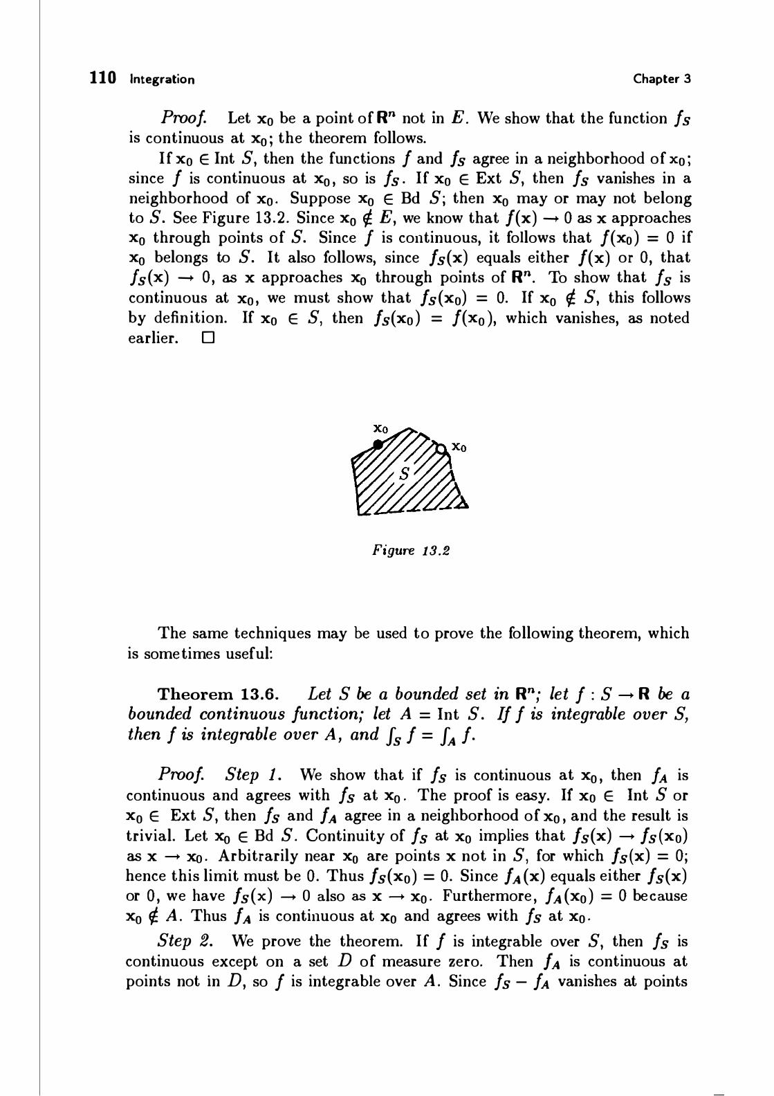
110 Integration Chapter 3
Proof. Let x0 be a point of R" not in E. We show that the function fs is continuous at x0 ; the theorem follows.
If x0 E Int S, then the functions f and /s agree in a neighborhood of xo ; since f is continuous at x0 , so is fs . If x0 E Ext S, then fs vanishes in a neighborhood of x0 • Suppose x0 E Bd S; then x0 may or may not belong to S. See Figure 13 .2 . Since x0 � E, we know that /(x) -+ 0 as x approaches x0 through points of S. Since f is continuous, it follows that /(xo) = 0 if x0 belongs to S. It also follows, since /s(x) equals either /(x) or 0, that fs(x) -+ 0, as x approaches x0 through points of R". To show that fs is continuous at x0 , we must show that /s(x0) = 0. If x0 � S, this follows by defin ition. If x0 E S, then /s(xo ) = /(x0 ), which vanishes, as noted earlier. 0
Figure 13.2
The same techniques may be used to prove the following theorem, which is sometimes useful:
Theorem 13.6. Let S be a bounded set in R"; let f : S -+ R be a bounded continuous function; let A = lnt S. If f is integrable over S, then f is integrable over A , and fs f = fA f.
Proof. Step 1. We show that if f s is continuous at x0 , then fA is continuous and agrees with f s at x0 • The proof is easy. If xo E lnt S or x0 E Ext S, then fs and /A agree in a neighborhood of x0 , and the result is trivial. Let x0 E Bd S. Continuity of fs at x0 implies that /s(x) -+ /s (xo) as x -+ xo . Arbitrarily near xo are points x not in S, for which /s(x) = 0; hence this limit must be 0. Thus /s(x0) = 0. Since /A (x) equals either /s(x) or 0 , we have /s(x) -+ 0 also as x -+ x0 • Furthermore , fA (xo ) = 0 because x0 � A . Thus /A is continuous at x0 and agrees with fs at x0 •
Step 2. We prove the theorem. If f is integrable over S, then fs is continuous except on a set D of measure zero. Then /A is continuous at points not in D, so f is integrable over A . Since fs - fA vanishes at points

§13. The Integral over a Bounded Set 111
not in D, we have JQ(fs - /A )
Then fs f = fA f. 0 0, where Q is a rectangle containing S.
EXERCISES
1 . Let f, g : S --+ R ; assume f and g are integrable over S. (a) Show that if f and g agree except on a set of measure zero, then
fs f = fs g.
(b) Show that if /(x) < g(x) for x E S and fs f = fs g, then f and g agree except on a set of measure zero.
2. Let A be a rectangle in Rk ; let B be a rectangle in Rn ; let Q = A x B. Let f : Q --+ R be a bounded function. Show that if JQ f exists, then
1 f(x, y) yEB
exists for x E A - D, where D is a set of measure zero in Rk. 3. Complete the proof of Corollary 13.4. 4. Let S1 and S2 be bounded sets in Rn; let f : S --+ R be a bounded
function. Show that if f is integrable over S1 and S2, then f is integrable over S1-S2 , and
1 f = 1 t - 1 f. s, - s2 s, s, n s2
5 . Let S be a bounded set in Rn; let f : S --+ R be a bounded continuous function; let A = Int S. Give an example where JA f exists and fs f does not.
6. Show that Theorem 13.6 holds without the hypothesis that f is continuous on S.
*7. Prove the following:
Theorem. Let S be a bounded set in Rn; let f : S --+ R be a bounded function. Let D be the set of points of S at which f fails to be continuous. Let E be the set of points of Bd S at which the condition
lim /(x) = 0 x-x0
fails to hold. Then fs f exists if and only if D and E have me asure zero. Proof (a) Show that /s is continuous at each point xo ¢ D U E. (b) Let B be the set of isolated points of S; then B C E because the
limit cannot be defined if xo is not a limit point of S. Show that if fs is continuous at Xo , then Xo ¢ D U (E - B) .
(c) Show that B is countable. (d) Complete the proof.

112 Integration Chapter 3
§14. RECTIFIABLE S ETS
We now extend the volume function, defined for rectangles , to more general subsets of R" . Then we relate this notion to integration theory, and extend the Fubini theorem to certain integrals of the form fs f.
Definition. Let S be a bounded set in R" . If the constant function 1 is integrable over S, we say that S is rectifiable, and we define the ( ndimensional) volume of S by the equation
v(S) = 1 1.
Note that this definition agrees with our previous definition of volume when S is a rectangle.
Theorem 14.1. A subset S of R"is rectifiable if and only if S is bounded and Bd S has measure zero.
Proof. The function 1s that equals 1 on S and 0 outside S is continuous on the open sets Ext S and Int S. It fails to be continuous at each point of Bd S. By Theorem 1 1 .2 , the function ls is integrable over a rectangle Q containing S if and only if Bd S has measure zero. 0
We list some properties of rectifiable sets.
Theorem 14.2. (a) (Positivity). If S is rectifiable, v(S) > 0. (b) (Monotonicity). If S1 and S2 are rectifiable and if S1 c S2 , then
v(SI ) < v(S2) . (c) (Additivity). If S1 and S2 are rectifiable, so are S1 U S2 and
sl n s2, and
v(S1 U S2) = v(S1 ) + v( S2) - v(S1 n S2 ) .
(d) Suppose S is rectifiable. Then v(S) = 0 if and only if S has measure zero.
(e) If S is rectifiable, so is the set A = Int S, and v(S) = v(A) . (f) If S is rectifiable, and if f : S --+ R is a bounded continuous
function, then f is integrable over S.
Proof. Parts (a) , (b) , and (c) follow from Theorem 13.3. Part (d) follows by applying Theorem 1 1 .3 to the non-negative function 15 . Part (e ) follows from Theorem 13.6, and (f) from Theorem 13 .5 . 0

§14. Rectifiable Sets 113
Let us make a remark on terminology. The concept of volume, as we have defined it, was called classically the theory of content (or Jordan content). This terminology distinguishes this concept from a more general one, called measure (or Lebesgue measure) . This concept is important in the development of an integral called the Lebesgue integral, which is a generalization of the Riemann integral.
Measure is defined for a larger class of sets than content is, but the two concepts agree when both are defined . A "set of measure zero" as we have defined it is in fact just a set whose Lebesgue measure exists and equals zero. Such a set need not of course be rectifiable.
A set whose Lebesgue measure is defined is usually called measurable. But there is no universally accepted corresponding term for a set whose Jordan content is defined. Some call such sets "Jordan-measurable" ; others refer to such sets as "domains of integration," because bounded continuous functions are integrable over such sets. One student suggested to me that a set whose Jordan content is defined should be called "contented" ! I have taken the term rectifiable, which is commonly used to refer to a curve whose length is defined, and have adopted it to refer to any set having volume (content) .
The class of rectifiable sets in Rn is not easy to describe other than by the condition stated in Theorem 14 .1 . It is tempting to think , for instance, that any bounde d open set in Rn, or any bounded closed set in Rn, should be rectifiable. That is not the case , as the following example shows:
EXAMPLE 1 . We construct a bounded open set A in R such that Bd A does not have measure zero.
The rational numbers in the open interval (0,1) are countable; let us arrange them in a sequence q1 , q2 , . • • • Let 0 < a < 1 be fixed. For each i, choose an open interval (a; , b;) of length less than a/2' that contains q; and is contained in (0,1) . These intervals will overlap, of course, but that doesn 't matter. Let A be the following open set of R:
We assume Bd A has measure zero and derive a contradiction. Set € = 1 - a. Since Bd A has measure zero, we may cover Bd A by countably many open intervals of total length less than €. Because A is a subset of [0, 1] that contains each rational in (0, 1 ) , we have A = [0, 1]. Since A = A U Bd A, the open intervals covering Bd A, along with the open intervals (a; , b; ) whose union is A, give an open covering of the interval (0,1]. The total length of the intervals covering Bd A is less than !, and the total length of the intervals covering A is less than 2::: a/2' = a. Because (0,1] is compact, it can be covered by finitely many of these intervals; the total length of these intervals is less than ! + a < 1 . This contradicts Corollary 10.5.
We conclude this section by discussing certain rectifiable sets that are especially useful ; they are called the "simple regions." For these sets, a version

114 Integration Chapter 3
of the Fubini theorem holds, as we shall see. We shall use these results only in the examples and the exercises.
Definition. Let C be a compact rectifiable set in R"- 1 ; let </>, '1/J : C --+ R be continuous functions such that </>(x) < '1/J(x) for x E C. The subset S of R" defined by the equation
S = {(x,t) I x E C and </>(x) < t < '1/J(x) }
is called a simple region in R" .
There is nothing special about the last coordinate here. If k + l = n - 1 , and if y and z denote the general points of Rk and Rl, respectively, then the set
S' = {(y,t , z) l (y , z) E C and </>(y, z) < t < '1/J(y , z)}
is also called a simple region in R".
*Lemma 14.3. and rectifiable.
If S is a simple region in R", then S is compact
Proof. Let S be a simple region, as in the definition. We show that S is compact and that Bd S has measure zero.
Step 1. The graph of </> is the subset of R" defined by the equation
G .p = {(x, t) I x E C and t = </>(x) } .
We show that Bd S lies in the union of the three sets G.p and G.p and
D = {(x,t) I x E Bd C and <J>(x) < t < '1/J(x) } .
Since each of these sets is contained in S, it follows that Bd S C S, so that S is closed . Being bounded, S is thus compact. See Figure 14. 1.
Suppose that (xo , to) belongs to none of the sets G.p, G.p , or D. We show that (x0 , t0) lies either in Int S or Ext S. As you can check, there are three possibilities:
( 1 ) x0 � C, (2) x0 E C and either t0 < </>(x0) or t0 > 'I/J(x0) , (3) xo E Int C and </>(xo ) < to < '1/J(xo ) .
In case (1 ) , there is a neighborhood U of x0 disjoint from C. Then U x R is disjoint from S, so that ( xo , t0 ) E Ext S.
Consider case (2). Suppose that t0 < </>(x0) . By continuity of <J>, we can choose a neighborhood lV of (x0 , to) such that the function <J>(x)- t is positive
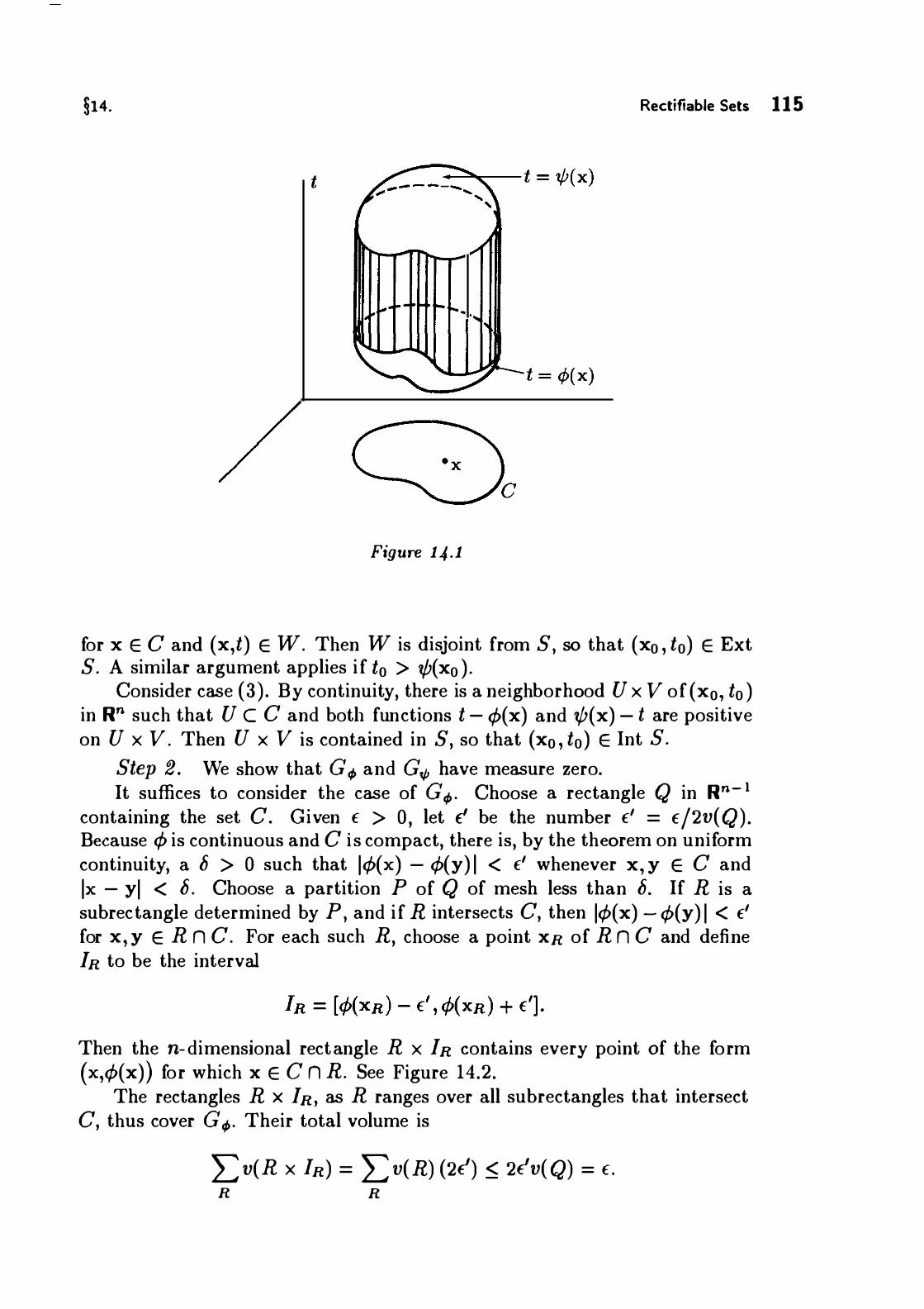
§14. Rectifiable Sets 115
t
Figure 14 .1
for x E C and ( x,t) E W. Then W is disjoint from S, so that ( x0 , t0) E Ext S. A similar argument applies if t0 > 'l/J(x0 ).
Consider case (3) . By continuity, there is a neighborhood U x V of (x0, t0 ) in Rn such that U C C and both functions t - ¢>(x) and '1/J(x) - t are positive on U x V. Then U x V is contained in S, so that (x0 , t0) E Int S.
Step 2. We show that G,p and G.p have measure zero. It suffices to consider the case of G <P · Choose a rectangle Q in Rn- I
containing the set C. Given E > 0, let E' be the number E1 = Ej2v(Q) . Because ¢> is continuous and C i s compact, there is, by the theorem on uniform continuity, a b > 0 such that 1</>(x) - </>(Y) I < E1 whenever x, y E C and lx - Yl < b . Choose a partition P of Q of mesh less than b. If R is a subrectangle determined by P, and if R intersects C, then 1</>(x) - <f>(y) I < E1 for x,y E R n C. For each such R, choose a point XR of R n C and define IR to be the interval
Then the n-dimensional rectangle R x IR contains every point of the form (x,</>(x)) for which X E c n R. See Figure 14.2.
The rectangles R X IR, as R ranges over all subrectangles that intersect C, thus cover G,p. Their total volume is
Lv(R x IR) = Lv(R) (2E') < 2E'v(Q) = E. R R

116 Integration
\..._ .... __ _ c
� Q
Figure 14.2
Chapter 3
Step 3. We show the set D has measure zero; then the proof is complete . Because ¢> and 1/J are continuous and C is compact, there is a number M such that
-M < </>(x) < 1/J( x) < M
for x E C. Given E > 0, cover Bd C by rectangles Q l ! Q2, . . . in R"- 1 of total volume less than E/2M . Then the rectangles Q; X [-M, M] in R" cover D and have total volume less than E. 0
*Theorem 14.4 (Fubini's theorem for simple regions). Let
S = { (x ,t) l x E C and ¢>(x) < t < '1/J(x)}
be a simple region in R". Let f : S -+ R be a continuous function. Then f is integrable over S, and
1 it =I/J(x) f(x,t).
xec t=if>(x)
Proof. Let Q x [-M, M] be a rectangle in R" containing S. Because f is continuous and bounded on S and S is rectifiable, f is integrable over S. Furthermore, for fixed x0 E Q, the function fs(x0 , t) is either identically zero

§14. Rectifiable Sets 1 17
(if x0 ¢ C), or it is continuous at all but two points of R . We conclude from Fubini 's theorem that
� is { lt =M fs(x,t) . lxEQ t =-M
Since the inner integral vanishes if x ¢ C, we can write this equation as
{ lt =M fs(x,t) . lxec t=-M
Furthermore, the number fs(x,t) vanishes unless ¢(x) < t < '1/J(x) , in which case it equals f(x,t) . Therefore we can write
1 lt =l/J(x) f(x,t) .
xEC t =</>(x) 0
The preceding theorem gives us a reasonable method for reducing the n-dimensional integral Is f to lower-dimensional integrals, at least if the integrand is continuous and the set S is a simple region .
If the set S is not a simple region, one can often in practice express S as a union of simple regions that overlap in sets of measure zero. Additivity of the integral tells us that we can evaluate the integral Is f by integrating over each of these regions separately and adding the results together. Just as in calculus, the procedure can be reasonably laborious . But at least it is straightforward.
Of course, there are rectifiable sets that cannot be broken up in this way into simple regions. Computing integrals over such sets is more difficult. One way of proceeding is to approximate S by a union of simple regions and follow a limiting procedure.

1 1 8 Integration Chapter 3
Figure 14 .3
EXAMPLE 2. Suppose one wishes to integrate a continuous function f over the set S in R2 pictured in Figure 14.3. While S is not a simple region, it is easy to break S up into simple regions that overlap in sets of measure zero, as indicated by the dotted lines.
EXAMPLE 3. Consider the set S in R2 given by
it is pictured in Figure 14.4 . While S is not a simple region, one can evaluate an integral over S by breaking S up into two simple regions that overlap in a set of measure zero, as indicated, and integrating over each of these regions separately. The limits of integration will be rather unpleasant, of course.
Now if one were actually assigned a problem like this in a calculus course, one would do no such thing! What one would do instead would be to express the integral in terms of polar coordinates, thereby obtaining an integral with much simpler limits of integration.
Expressing a two-dimensional integral in terms of polar coordinates is a special case of a quite general method for evaluating integrals, which is called "substitution" or "change of variables." We shall deal with it in the next chapter.
Figure 14 .4
Let us make one final remark . There is one thing lacking in our discussion of the notion of volume. How do we know that the volume of a set is independent of its position in space? Said differently, if S is a rectifiable set,

§14. Rectifiable Sets 119
and if h : nn -+ nn is a rigid motion (whatever that means) , how do we know that the sets S and h(S) have the same volume?
For example, each of the sets S and T pictured in Figure 14 .5 represents a square with edge length 5 ; in fact T is obtained by rotating S through the angle (} = arctan 3/4. It is immediate from the definition that S has volume 25 . It is clear that T is rect ifiable, for it is a simple region. Bu.t how do we know T has volume 25?
( -3, 4)
(5 , 0)
Figure 14 .5
One can of course simply calculate v(T) . One way to proceed is to write equations for the functions '1/J(x) and </>(x) whose graphs bound T above and below respectively, and to integrate the function '1/J(x) - </>( x) over the interval [-3 , 4] . See Figure 14 .6.
Another way to proceed is to enclose T in a rectangle Q, take a partition P of Q , and calculate the upper and lower sums of the function 1r with respect to P . The lower sum equals the total area of all subrectangles contained in T,
� y = '1/J(x)
- 3 4
Figure 14 .6

12 0 Integration Chapter 3
while the upper sum equals the total area of all subrectangles that intersect T. One needs to show that
L( lr , P) < 25 < U(lr , P)
for all P. See Figure 14.7 . Neither of these procedures is especially appealing! What one needs is a
general theorem. In the next chapter, we shall prove the following result: Suppose h : Rn -+ nn is a function satisfying the condition
I I h(x) - h(y) l l = I I x - Y I I
for all x, y E Rn ; such a function is called an isometry. If S is a rectifiable set in Rn , then the set T = h(S) is also rectifiable, and v(T) = v(S).
EXERCISES
�V' ��v !JVj � 1/; ��/;, '11 '1Pl 'JJ � v.A'I. 'JJ, VI '//,'liV ·;1/1� �II I l'r7!i-', /.L. / · V '/ .J.,/r �.!' 1 l / rl /, 'I '/. \ 1-"l_l-ih'i ��Ji.�V/1� 1. V//, '!1ft "" 11 rr. /. '/ / (..l.JT 'J. 7. '\:IT V. /� �.�/f',.J
/ � 1/ �//Jill�'/ ' VJI ill VJ'fJV/, i\�' 'JVfiiJ,r;Y/, Figure 14 .7
1 . Let S be a bounded set in Rn that is the union of the countable collection of rectifiable sets s. ' s2 ' . . . . (a) Show that S1 U · · · U Sn is rectifiable.
(b) Give an example showing that S need not be rectifiable.
2 . Show that if S1 and S2 are rectifiable, so is S1 - S2 , and
3. Show that if A is a nonempty, rectifiable open set in Rn, then v(A) > 0.
4. Give an example of a bounded set of measure zero that is rectifiable, and an example of a bounded set of measure zero that is not rectifiable.
5. Find a bounded closed set in R that is not rectifiable.

§15. Improper Integrals 121
6 . Let A be a bounded open set in Rn; let f : Rn --+ R be a bounded continuous function. Give an example where f"A f exists but JA f does not.
7. Let S be a bounded set in Rn. (a) Show that if S is rectifiable, then so is the set S, and v(S) = v( S) . (b) Give an example where S and Int S are rectifiable, but S is not .
8 . Let A and B be rectangles in Rk and Rn , respectively. Let S be a set contained in A x B. For each y E B, let
S11 = {x I x e A and (x, y) E S} .
We call S11 a cJ•oss-section of S . Show that if S is rectifiable, and if S11 is rectifiable for each y E B, then
v(S) = 1 v(S11) . yEB
§15. I MPROPER INTEGRALS
We now extend our notion of the integral. We define the integral fs f in the case where S is not necessarily bounded and f is not necessarily bounded. Such an integral is sometimes called an improper integral.
We shall define our extended notion of the integral only in the case where s is open in nn .
Definition. Let A be an open set in Rn; let f : A -+ R be a continuous function. If f is non-negative on A, we define the (extended) integral of f over A, denoted JA f , to be the supremum of the numbers fv f , as D ranges over all compact rectifiable subsets of A , provided this supremum exists. In this case, we say that f is integrable over A (in the extended sense) . More generally, if f is an arbitrary continuous function on A, set
f+ (x) = max{f(x), 0} and J_ (x) = max{-f(x) , 0} .
We say that f is integrable over A (in the extended sense) if both f+ and f _ are; and in this case we set
where JA denotes the extended integral throughout.

122 Integration Chapter 3
If A is open in nn and both f and A are bounded , we now have two different meanings for the symbol fA f. It could mean the extended integral, or it could mean the ordinary integral . It turns out that if the ordinary integral exists, then so does the extended integral and the two integrals are equal. Nevertheless , some ambiguity persists, because the extended integral may exist when the ordinary integral does not. To avoid ambiguity, we make the following convention :
Convention. If A is an open set in Rn , then fA f will denote the extended integral unless specifically stated otherwise.
Of course, if A is not open , there is no ambiguity; fA f must denote the ordinary integral in this case.
We now give a reformulation of the definition of the extended integral that is convenient for many purposes. It is related to the way improper integrals are defined in calculus. We begin with a preliminary lemma:
Lemma 15.1. Let A be an open set in nn . Then there exists a sequence C. , C2, • • • of compact rectifiable subsets of A whose union is A, such that eN c lot CN+I for each N .
Proof. Let d denote the sup metric d(x, y) = !x - yl on Rn . If B c nn, let d(x, B) denote the distance from x to B, as usual . (See §4.)
Now set B = nn - A. Then given a positive integer N , let DN denote the set
DN = {x I d(x,B) > 1/N and d(x, O) < N}.
Since d(x,B) and d(x, 0) are continuous functions of x (see the proof of Theorem 4.6) , DN is a closed subset of Rn . Because DN is contained in the cube of radius N centered at 0, it is bounded and thus compact. Also, DN is contained in A, since the inequality d(x,B) > 1/N implies that x cannot be in B . To show the sets D N cover A, let x be a point of A. Since A is open , d(x,B) > 0; then there is an N such that d(x,B) > 1/N and d(x, O) < N, so that x E D N. Finally, we note that the set
AN+I = {x I d(x ,B) > 1/(N + 1) and d(x, O) < N + 1 }
is open (because d(x,B) and d(x , 0) are continuous) . Since AN +I is contained in D N + 1 and contains D N by definition , it follows that D N C lot D N +I . See Figure 15 . 1 .
The sets DN are not quite the sets we want, since they may not be rectifiable. We construct the sets C N as follows: For each x E D N, choose a closed cube that is centered at x and is contained in lot D N + 1 . The interiors of these cubes cover D N; choose finitely many of them whose interiors cover

§15. Improper Integrals 123
Figure 1 5. 1
D N and let their union be C N. Since C N is a finite union of rectangles, it is compact and rectifiable. Then
It follows that the union of the sets eN equals A and that eN c Int CN+l for each N. 0
Now we obtain our alternate formulation of the definition :
Theorem 15.2. Let A be open in Rn; let f : A -+ R be continuous. Choose a sequence C N of compact rectifiable subsets of A whose union is A such that CN C lot CN+I for each N. Then f is integrable over A if and only if the sequence feN lfl is bounded. In this case,
r f = lim r f. }A N-+oo leN
It follows from this theorem that f is integrable over A if and only if lfl is integrable over A .
Proof. Step 1. We prove the theorem first in the case where f is non-negative. Here f = l f l . Since the sequence feN f is increasing (by monotonicity) , it converges if and only if it is bounded.

124 Integration Chapter 3
Suppose first that f is integrable over A. If we let D range over all compact rectifiable subsets of A, then
since C N is itself a compact rectifiable subset of A. It follows that the sequence feN f is bounded, and
lim r f < r f. N-+oo leN }A Conversely, suppose the sequence feN f is bounded . Let D be an arbi
trary compact rectifiable subset of A. Then D is covered by the open sets
Int C1 C Int C2 C · · · , hence by finitely many of them, and hence by one of them, say Int C M . Then
r f < r f < lim r f. lv leM N-+oo leN Since D is arbitrary, it follows that f is integrable over A, and
r f < lim r f. }A N-+oo leN
Step 2. Now let f : A -+ R be an arbitrary continuous function . By definition, f is integrable over A if and only if f+ and f _ are integrable over A; this occurs if and only if the sequences feN f+ and feN f- are bounded, by Step 1. Note that
while
0 < f+(x) < lf(x) l and 0 < f- (x) < l f(x) l ,
lf(x) l = f+(x) + f_ (x) .
It follows that the sequences feN f + and feN f _ are bounded if and only if the sequence feN lf l is bounded . In this case, the former two sequences converge to fA f + and fA f _ , respectively. Since convergent sequences can be added term-by-term, the sequen ce
converges to fA f+ - fA f- ; and the latter equals fA f by definition . 0
We now verify the properties of the extended integral; many are analogous to those of the ordinary integral . Then we relate the extended integral to the ordinary integral in the case where both are defined .

§15. Improper Integrals 125
Theorem 15.3. Let A be an open set in nn . Let j, g : A -+ R be continuous functions.
(a) (Linearity) . Iff and g are integrable over A, so is af + bg; and
l (af + bg)
(b) (Comparison) . Let f and g be integrable over A. If f(x) < g(x) for x E A, then
In particular,
(c) (Monotonicity) . Assume B is open and B C A. If f is nonnegative on A and integrable over A, then f is integrable over B and
(d) (Additivity) . Suppose A and B are open in nn and f is continuous on A U B. If f is integrable on A and B, then f is integrable on A U B and A n B, and
r 1 = r 1 + r 1 _ r r lAuB }A jB lAnB
Note that by our convention, the integral symbol denotes the extended integral throughout the statement of this theorem.
Proof. Let C N be a sequence of compact rectifiable sets whose union is A, such that eN c Int CN+l for all N.
(a) We have
<
by the comparison and linearity properties of the ordinary integral . Since both sequences fe lf l and fe lgl are bounded, so is fe laf + bgl . Linearity now follows by taking limits i� the equation
N
r (af + bg) leN + b r 9 . leN

126 Integration Chapter 3
(b) If f(x) < g(x) , one takes limits in the inequality
(c) If D is a compact rectifiable subset of B, then D is also a compact rectifiable subset of A, so that
by definition . Since D is arbitrary, f is integrable over B and J8 f < JA f. (d) Let D N be a sequence of compact rectifiable sets whose union is B
such that DN C lot DN+l for each N. Let
EN = C N U D N and F N = C N n D N.
Then EN and F N are sequences of compact rectifiable sets whose unions equal A U B and A n B, respectively. See Figure 15.2.
Figure 15.2
We show EN C lot EN+1 and FN C lot FN+1 • lf x E EN , then x is in either C N or D N. If the former, then some neighborhood of x is contained in CN+ l · If the latter, some neighborhood of x is contained in DN+l · In either case, this neighborhood of x is contained in EN+1 , so that x E lot EN+1 •
Similarly, if x E FN , then some neighborhood U of x is contained in C N + 1 , and some neighborhood of V of x is contained in D N +1 . The neighborhood U n V of x is thus contained in FN+1 , so that x E lot FN+1 •

§15. Improper Integrals 127
Additivity of the ordinary integral tells us that
Applying this equation to the function lf l , we see that fEN lf l and fFN lfl are bounded above by
Thus f is integrable over A U B and A n B. The desired equation now follows by taking limits in ( * ) . 0
Now we relate the extended integral to the ordinary integral .
Theorem 15.4. Let A be a bounded open set in nn; let f : A -+
R be a bounded continuous function. Then the extended integral fA f exists. If the ordinary integral fA f also exists, then these two integrals are equal.
Proof. Let Q be a rectangle containing A.
Step 1. We show the extended integral of f exists. Choose M so that lf(x) l < M for x E A. Then for any compact rectifiable subset D of A,
L lf l < L M < M · v(Q).
Thus f is integrable over A in the extended sense. Step 2. We consider the case where f is non-negative. Suppose the
ordinary integral of f over A exists. It equals, by definition , the integral over Q of the function fA . If D is a compact rectifiable subset of A, then
L f = L fA because f = fA on D,
< � fA by monotonicity,
= (ordinary) l f.
Since D is arbitrary, it follows that
(extended) l f < (ordinary) l f.

12 8 Integration Chapter 3
Figure 15.3
On the other hand, let P be a partition of Q, and let R denote the general subrectangle determined by P. Denote by R. , . . . , R�c those subrectangles that lie in A, and let D = R1 U · · · U R�c . See Figure 15.3. Now
k L(JA , P) = L fiR; (f) · v(R; ) ,
i = I
because fiR(! A) = fiR(!) if R is contained in A and fiR(! A ) = 0 if R is not contained in A. On the other hand,
k L fiR; (f) · v(R;) < by the comparison property, i=l
by additivity,
< (extended) L f by definition.
Since P is arbitrary, we conclude that
(ordinary) L f < (extended) L f.
Step 3. Now we consider the general case. Write f = f + - f _ , as usual. Since f is integrable over A in the ordinary sense , so are f + and f _ , by

§15. Improper Integrals 129
Lemma 13.2. Then
(ordinary ) L f = (ordinary) L f+ - (ordinary ) L !
(extended) L f+ - (extended) L !
by linearity,
by Step 2 ,
(extended) L f by definition. 0
EXAMPlE 1 . If A is a bounded open set in Rn and f : A --+ R is a bou nded continuous function, then the extended integral fA f exists, but the ordinary integral fA f may not. For example, let A be the open subset of R constructed in Example 1 of §14 . The set A is bounded, but Bd A does not have measure zero. Then the ordinary integral fA 1 does not exist, although the extended integral fA 1 does.
A consequence of the preceding theorem is the following:
Corollary 15.5. Let S be a bounded set in nn; let f : S -+ R be a bounded continuous function. If f is integrable over S in the ordinary sense, then
(ordinary) 1 f (extended) r f. Jlnt S
Proof. One applies Theorems 13 .6 and 15.4. 0
This corollary tells us that any theorem we prove about extended integrals has implications for ordinary integrals. The change of variables theorem, which we prove in the next chapter, is an important example.
We have already given two formulations of the definition of the extended integral, and we will give another in the next chapter. All these versions of the definition are useful for different theoretical purposes. Actually applying them to computational problems can be a bit awkward, however. Here is a formulation that is useful in many practical situations. We shall use it in some of the examples and exercises:

130 Integration Chapter 3
*Theorem 15.6. Let A be open in R"; let f : A --+ R be continuous. Let U1 c U2 c · · · be a sequence of open sets whose union is A. Then fA f exists if and only if the sequence fuN lf l exists and is bounded; in this case,
r f = lim r f. }A N-oo luN Proof. It suffices, as usual, to consider the case where f is non-negative. Suppose the integral fA f exists. Monotonicity of the extended integral
implies that f is integrable over UN and that for each N,
It follows that the increasing sequence fuN f converges, and that
lim 1 f < r f. N-oo UN }A Conversely, suppose the sequence fuN f exists and is bounded. Let D
be a compact rectifiable subset of A. Since D is covered by the open sets ul c u2 c 0 0 0 , it is covered by finitely many of them, and hence by one of them, say UM · Then , by definition ,
Since D is arbitrary,
In applying this theorem, we usually choose UN so that it is rectifiable and f is bounded on UN; then the integral fuN f exists as an ordinary integral (and hence as an extended integral) and can be computed by familiar techniques. See the examples following.

§15. Improper Integrals 131
EXAMPlE 2. Let A be the open set in R2 defined by the equation
A = { (x, y) l x > I and y > l } .
Let f(x, y) = 1 /x2y2 • Then f is bounded on A, but A is unbounded. We could use Theorem 15.2 to calculate fA /, by setting eN = [(N + 1 )/ N, N]2 and integrating f over eN. It is a bit easier to use Theorem 15.6, setting UN = ( 1 , N)2 and integrating f over UN . See Figure 15.4. The set UN is rectifiable; f is bounded on UN because UN is compact and f is continuous on UN. Thus fuN f exists as an ordinary integral , so we can apply the Fubini theorem. We compute
We conclude that fA f = 1 .
1 N
Figure 1 5.4
B
I/N 1
Figure 1 5. 5
EXAMPlE 3. Let B = (0, 1 ) 2 ; let f(x, y) = 1/x2y2 , as before. Here B is bounded but f is not bounded on B; indeed, f is unbounded near each point of the x and y axes. However, if we set UN = (I jN, I?, then f is bounded on UN. See Figure 15.5 . We compute
We conclude that f8 f does not exist.

132 Integration Chapter 3
EX ERCISES
1 . Let f : R --+ R be the function f (x) = x. Show that, given >. E R, there exists a sequence CN of compact rectifiable subsets of R whose union is R , such that eN c Int CN+I for each N and
Does the extended integral f. f exist?
2. Let A be open in Rn; let J, g : A --+ R be continuous; suppose that lf (x) l < g(x) for x E A. Show that if L g exists, so does L f. (This result is analogous to the so-called "comparison test" for the convergence of an infinite series. )
3. (a) Let A and B be the sets of Examples 2 and 3; let f(x, y) = 1/(xy)1/2 • Determine whether fA f and fB f exist; if either does , calculate it.
(b) Let C = { (x , y) I x > 0 and y > 0} . Let
f (x, y) = 1 /(x2 + Vx) (y2 + ../Y).
Show that fc f exists; do not attempt to calculate it.
4. Let f(x, y) = 1/(y + 1 )2 • Let A and B be the open sets
A = { ( x, y) I x > 0 and x < y < 2x } ,
B = { (x , Y) I x > 0 and x2 < y < 2x2 } ,
of R2• Show that fA f does not exist; show that fB f does exist and calculate it. See Figure 15.6.
Figure 1 5.6
§15.
5. Let f(x, y) = 1lx (xy)1 12 for x > 0 and y > 0. Let
Improper Integrals 133
Ao = {( x, y) I 0 < x < 1 and x < y < 2x} , Bo = { (x , y) I 0 < x < 1 and x2 < y < 2x2 } .
Determine whether JAo f and JBo f exist; if so, calculate.
6. Let A be the set in R2 defined by the equation
A = { (X, y) I X > 1 and 0 < Y < 1 I X} . Calculate L 1 I xy1 12 if it exists.
*7. Let A be a bounded open set in Rn; let f : A --+ R be a bounded continuous function. Let Q be a rectangle containing A. Show that
*8. Let A be open in Rn. We say f : A --+ R is locally bounded on A if each x in A has a neighborhood on which f is bounded. Let F(A) be the set of all functions f : A --+ R that are locally bounded on A and continuous on A except on a set of measure zero.
(a) Show that if f is continuous on A, then f E F(A) . (b) Show that if f is in F(A), then f is bounded on each compact subset
of A and the definition of the extended integral L f goes through without change.
(c) Show that Theorem 15.3 holds for functions f in F(A). (d) Show that Theorem 1 5.4 holds if the word "continuous" in the hy
pothesis is replaced by "continuous except on a set of measure zero."


Change of Variables
In evaluating the integral of a function of a single variable, one of the most useful tools is the so-called "substitution rule ." It is used in calculus, for example, to evaluate such an integral as
one makes the substitution y = 2x2 + 1 , reducing this integral to the integral
which is easy to evaluate. (Here we use the "dx" and "dy" notation of calculus.)
Our intention in this chapter is to generalize the substitution rule in two ways:
( 1) We shall deal with n-dimensional integrals rather than one-dimensional integrals.
(2) We shall prove it for the extended integral , rather than merely for integrals of bounded functions over bounded sets. This will require us to limit ourselves to integrals over open sets in Rn, but , as Corollary 15.5 shows, this is not a serious restriction .
We call the generalized version of the substitution rule the change of variables theorem.
135

136 Change of Variables Chapter 4
§ 16. PARTIT IONS OF U N ITY
In order to prove the change of variables theorem, we need to reformulate the definition of the extended integral fA f. This integral is obtained by breaking the set A up into compact rectifiable sets C N, and taking the limit of the corresponding integrals feN f . In our new approach, we instead break the function f up into functions f N , each of which vanishes outside a compact set, and we take the limit of the corresponding integrals fA f N . This approach has many advantages, especially for theoretical purposes; it will recur throughout the rest of the book.
This approach involves a notion of comparatively recent origin in mathematics, called a "partition of unity," which we define in this section .
We begin with several lemmas.
Lemma 16.1. Let Q be a rectangle in R" . There is a coo function </> : R" --+ R such that </>(x) > 0 for x E lot Q and </>(x) = 0 otherwise.
Proof. Let f : R -+ R be defined by the equation { e- l/:r: f(x) =
0
if X > 0,
otherwise.
Then f(x) > 0 for X > 0. It is a standard result of single-variable analysis that f is of class coo . (A proof is outlined in the exercises.) Define
g(x) = f(x) · f( 1 - x).
Then g is of class C00 ; furthermore, g is positive for 0 < x < 1 and vanishes otherwise. See Figure 16 . 1 . Finally, if
y = /(x) y = g(x)
1
Figure 1 6. 1

§16. Partitions of Unity 137
define
Lemma 16.2. Let A be a collection of open sets in R" ; let A be their union. Then there exists a countable collection Q 1 , Q2 , . . • of rectangles contained in A such that:
( 1) The sets lot Q; cover A.
(2) Each Q; is contained in an element of A. (3) Each point of A has a neighborhood that intersects only finitely
many of the sets Q;.
Proof. It is not difficult to find rectangles Q; satisfying ( 1) and (2). Choosing them so they also satisfy (3) , the so-called "local finiteness condition," is more difficult.
Step 1 . Let D1 , D2, • • • be a sequence of compact subsets of A whose union is A , such that D; C lot D;+I for each i . For convenience in notation, let D; denote the empty set for i < 0. Then for each i , define
B; = D; - lot D;_1 • The set B; is bounded, being a subset of D;; and it is closed, being the
intersection of the closed sets D; and R" - lot D;- 1 . Thus B; is compact. Also, B; is disjoint from the closed set Di-2, since Di-2 C lot D;_ 1 • For each x E B;, we choose a closed cube Cx centered at x that is contained in A and is disjoint from D;-2; also choose Cx small enough that it is contained in an element of the collection of open sets A. See Figure 16.2 .
Figure 1 6.2

138 Change of Variables Chapter 4
The interiors of the cubes Cx cover B; ; choose finitely many of these cubes whose interiors cover B;; let C; denote this finite collection of cubes. See Figure 16.3 .
Figure 1 6.3
Step 2. Let C be the collection
C;
then C is a countable collection of rectangles (in fact, of cubes) . We show this collection satisfies the requirements of the lemma.
By construction , each element of C is a rectangle contained in an element of the collection A. We show that the interiors of these rectangles cover A. Given x E A, let i be the smallest integer such that x E lot D;. Then x is an element of the set B; = D; - lot D;- 1 • Since the interiors of the cubes belonging to the collection C; cover B;, the point x lies interior to one of these cubes.
Finally, we check the local finiteness condition . Given x, we have x E lot D; for some i. Each cube belonging to one of the collections C;+2 , C;+3 , . . • is disjoint from D;, by construction . Therefore the open set lot D; can intersect only the cubes belonging to one of the collections cl ' 0 0 0 ' C;+I 0 Thus X has a neighborhood that intersects only finitely many cubes from the collection C. 0
We remark that the local finiteness condition holds for each point x of A, but it does not hold for a point x of Bd A. Each neighborhood of such a point necessarily intersects infinitely many of the cubes from the collection C, as you can check.

§16. Partitions of Unity 139
Definition. If </> : Rn --+ R, then the support of </> is defined to be the closure of the set { x I </>( x) f:. 0} . Said differently, the support of </> is characterized by the property that if x ¢ Support </>, then there is some neighborhood of x on which the function </> vanishes identically.
Theorem 16.3 (Existence of a partition of unity). Let A be a collection of open sets in nn ; let A be their union. There exists a sequence </>1 , </>2 , • • . of continuous functions </>; : Rn --+ R such that:
( 1) </>; (x) > 0 for all x. (2) The set S; = Support </>; is contained in A.
(3) Each point of A has a neighborhood that intersects only finitely many of the sets S; .
(4) .L� 1 </>;(x) = 1 for each x E A .
(5) The functions </>; are of class coo. (6) The sets S; are compact. (7) For each i, the set S; is contained in an element of A.
A collection of functions {</>;} satisfying conditions ( 1)-(4) is called a partition of unity on A. If it satisfies (5), it is said to be of class coo ; if it satisfies (6), it is said to have compact supports; if it satisfies (7), it said to be dominated by the collection A.
Proof. Given A and A, let Q1 , Q2, . . . be a sequence of rectangles in A satisfying the conditions stated in Lemma 16 .2. For each i, let 1/J; : Rn -+ R be a C00 function that is positive on lot Q; and zero elsewhere. Then 1/J;(x) > 0 for all x. Furthermore, Support 1/J; = Q; ; the latter is a compact subset of A that is contained in an element of A. Finally, each point of A has a neighborhood that intersects only finitely many of the sets Q;. The collection {1/J; } thus satisfies all the conditions of our theorem except for (4) .
Condition (3) tells us that for x E A, only finitely many of the numbers 1/J1 (x), 1/J2(x), . . . are non-zero. Thus the series
00 A(x) = L 1/J;(x)
i= l
converges trivially. Because each x E A has a neighborhood on which A(x) equals a finite sum of C00 functions, A(x) is of class C00 • Finally, A(x) > 0 for each x E A; given x, there is a rectangle Q; whose interior contains x, whence 1/J; (x) > 0. We now define
</>; (x) = 1/J;(x)/ A(x);
the functions </>; satisfy all of the conditions of our theorem. 0

140 Change of Variables Chapter 4
Conditions ( 1) and (4) imply that, for each x E A, the numbers </>; (x) actually "partition unity," that is, they express the unity element 1 as a sum of non-negative numbers. The local finiteness condition (3) has the consequence that for any compact set C contained in A, there is an open set about C on which </>; vanishes identically except for finitely many i. To find such an
open set, one covers C by finitely many neighborhoods , on each of which </>; vanishes except for finitely many i ; then one takes the union of this finite collection of neighborhoods.
EXAMPlE 1 . Let f : R --+ R be defined by the equation { ( 1 + cos x)/2 for -1r < x < 1r, f(x) =
0 otherwise.
Then f is of class C 1 • For each integer m > 0, set </>2m+l (x) = f(x - m1r). For each integer m > 1 , set </>2m(x) = f(x + m1r). Then the collection {¢; } forms a partition of unity on R . The support S; of ¢; is a closed interval of the form [k1r, (k+2)7r] , which is compact, and each point of R has a neighborhood that intersects at most three of the sets S; . We leave it to you to check that l: <f>; (x) = 1 . Thus {¢; } is a partition of unity on R. See Figure 16.4.
- 27r - 1r
Figure 1 6.4
Now we explore the connection between partitions of unity and the extended integral. We need a preliminary lemma:
Lemma 16.4. Let A be open in R"; let f : A --+ R be continuous. Iff vanishes outside the compact subset C of A, then the integrals fA f and fc f exist and are equal.

§16. Partitions of Unity 141
Proof. The integral fc f exists because C is bounded, and the function fc' which equals f on A and vanishes outside C, is continuous and bounded on all of nn.
Let C; be a sequence of compact rectifiable sets whose union is A, such that C; C lot C;+I for each i. Then C is covered by finitely many sets lot C;, and hence by one of them, say lot eM . Since f vanishes outside C,
r J = r J lc leN
for all N > M. Applying this fact to the function lf l shows that lim fcN lfl exists, so that f is integrable over A; applying it to f shows that fc f = lim feN f = fA f. 0
Theorem 16.5. Let A be open in nn; let f : A --+ R be continuous. Let { </>;} be a partition of unity on A having compact supports. The integral fA f exists if and only if the series
converyes; in this case,
Note that the integral fA </>d exists and equals the ordinary integral fs, </>;J (where S; = Support </>;) by the preceding lemma.
Proof. We consider first the case where f is non-negative on A. Step 1 . Suppose f is non-negative on A, and suppose the senes
.L[JA </>;!] converges. We show that fA f exists and
Let D be a compact rectifiable subset of A. There exists an M such that for all i > M, the function </>; vanishes identically on D. Then
M f(x) = L </>;(x)f(x)
i:I

142 Change of Variables
for x E D. We conclude that
M 1 f = L [1 </>if] by linearity, D i = I D
M < E [1 </>;!] by monotonicity,
i : I DUS;
M
= L [1 </>;!] by the preceding lemma, i : I A
It follows that f is integrable over A, and
Chapter 4
Step 2. Suppose f is non-negative on A, and suppose f is integrable over A . We show the series E[JA </>;!] converges , and
Given N, the set D = sl u . . . u SN is compact. Furthermore, for i = 1 , . . . , N , the function </>d vanishes outside D, so that
by the preceding lemma. We conclude that
N N
2: [1 <f>;f1 = 2: [1 <f>;f1 i : I A i=I D
N == 1 [E </>; J] by linearity,
D i : I
< l f by the comparison property,
§16. Partitions of Unity 143
Thus the series .L [fA </>;/] converges because its partial sums are bounded, and its sum is less than or equal to fA f.
The theorem is now proved for non-negative functions f. Step 3. Consider the case of an arbitrary continuous function f : A --+
R . By Theorem 15 .2 , the integral fA f exists if and only if the integral fA lfl exists, and this occurs if and only if the series
converges, by Steps 1 and 2 . On the other hand, if fA f exists, then
l f = l f+ - l f- by definition ,
= f: [1 </>;/+] - f: [1 </>d- ] by Steps 1 and 2 , i : I A i : I A
= f: [1 </>d] by linearity, i=I A
since convergent series can be added term-by-term. 0
EXERCISES
1 . Prove that the function f of Lemma 16 . 1 is of class C00 as follows: Given any integer n > 0, define /n : R --+ R by the equation { (e-lf:r)/xn for x > 0, fn(x) =
0 for x < 0.
(a) Show that /n is continuous at 0. [Hint: Show that a < ea for all a. Then set a = tj2n to conclude that
Set t = 1/x and let X approach 0 through positive values.]
(b) Show that /n is differentiable at 0.
(c) Show that f�(x) = fn+2 (x) - nfn+l (x) for all x. (d) Show that f n is of class C00 •

144 Change of Variables Chapter 4
2 . Show that the functions defined in Example 1 form a partition of unity on R. [Hint: Let fm (x) = f(x - m1r), for all integers m. Show that l:f2m(x) = (1 + cos x)/2. Then find l:: hm+ I (x).]
3. (a) Let S be an arbitrary subset of Rn; let Xo E S. We say that the function f : s --+ R is differentiable at Xo , of class cr, provided there is a cr function g : u --+ R defined in a neighborhood u of Xo in Rn, such that g agrees with f on the set U n S. In this case, show that if ¢ : Rn ..... R is a cr function whose support lies in U, then the function { ¢(x)g(x)
h(x) = 0
for x E U,
for x ¢ Support ¢,
is well-defined and of class cr on Rn. (b) Prove the following:
Theorem. If f : S ..... R and f is differentia ble of class cr at ea ch point Xo of S, then f may be extended to a cr function h : A --+ R that is defined on an open set A of Rn containing S.
[Hint: Cover S by appropriately chosen neighborhoods, let A be their union , and take a C00 partition of unity on A dominated by this collection of neighborhoods.]
§17. THE CHANGE OF VA RIABLES THEO REM
Now we discuss the general change of variables theorem. We begin by reviewing the version of it used in calculus; although this version is usually proved in a first course in single-variable analysis, we reprove it here.
Recall the common convention that if f is integrable over [a , b] , then one defines
Theorem 11.1 (Substitution rule). Let I = [a, b] . Let g : I --+ R be a function of class C1 , with g'(x) :f. 0 for x E (a, b) . Then the set g(I) is a closed interval J with end points g(a) and g(b) . If f : J --+ R is continuous, then
f = r u 0 g)g' , 1g(b) b
g(a) la

§17. The Change of Variables Theorem 145
or equivalently, 1 1 = 1u o g) lg' l ·
Proof. Continuity of g' and the intermediate-value theorem imply that either g'( x) > 0 or g' (x) < 0 on all of (a, b) . Hence g is either strictly increasing or strictly decreasing on /, by the mean-value theorem, so that g is one-to-one. In the case where g' > 0 , we have g(a) < g(b) ; in the case where g' < 0, we have g(a) > g(b) . In either case, let J = [c, d] denote the interval with end points g(a) and g(b) . See Figure 17 .1 . The intermediatevalue theorem implies that g carries I onto J. Then the composite function f(g( x)) is defined for all x in [a , b] , so the theorem at least makes sense .
d d
c c
a b a b g' > 0 g' < 0 Figure 1 7. 1
Define F(y) = ly J
for y in [c, d] . Because f is continuous, the fundamental theorem of calculus implies that F'(y) = f(y) . Consider the composite function h(x) = F(g(x)) ; we differentiate it by the chain rule. We have
h'(x) = F'(g(x))g' (x) = J (g(x)) g'(x) .
Because the latter function is continuous, we can apply the fundamental theorem of calculus to integrate it. We have x:b 1=a f(g(x))g'(x) = h(b) - h(a)
= F(g(b)) - F(g(a))
lg(b) = f c lg(a) f.
c

146 Change of Variables Chapter 4
Now c equals either g(a) or g(b) . In either case, this equation can be written in the form
1b lg(b) (f 0 g)g' = f. a g(a)
This is the first of our desired formulas. Now in the case where g' > 0, we have J = [g(a) , g(b)] . Since lg' l = g'
in this case, equation ( *) can be written in the form
In the case where g' < 0, we have J = [g(b) , g(a)]. Since lg' l = -g' in this case, equation (*) can again be written in the form (**)· 0
EXAMPlE 1 . Consider the integral
Set f(y) = y10 and g(:z:) = 2x2 + 1 . Then g'(x) = 4x, which is positive for 0 < x < 1 . See Figure 17 .2. The substitution rule implies that
1
1 7r/2
Figure 1 7.2 Figure 17.3
§17.
EXAMPlE 2. Consider the integral ill 1
1 1/( 1 - y2 ) 1 /2 .
The Change of Variables Theorem 147
In calculus one proceeds as follows: Set y = g(x) = sin x for -7r/2 < x < 1rj2. Then g'(x) = cos x, which is positive on (-7r/2 , 7r/2) and satisfies the conditions g(-7r/2) = -1 and g(7r/2) = 1 . See Figure 17.3. If f(y) is continuous on the interval [-1 , 1], then the substitution rule tells us that
11 f = 1"''2 (f 0 g)g' . -1 -Tr/2
Applying this rule to the function f(y) = 1/( 1 - y2 ) 112 , we have
11 I/(1 - y2 )1 /2 = 1"''2 [1/(1 - sin2 x )1 '2] cos x = 1"''2 1 = 7r. -1 -Tr/2 -Tr/2
Thus the problem seems to be solved. However, there is a difficulty here. The substitution rule does not apply in
this case, for the function f(y) is not continuous on the interval -1 < y < I ! The integral of f is in fact an improper integral, since f is not even bounded on the interval (-1, 1) .
As indicated earlier, we shall generalize the substitution rule to n-dimensional integrals , and we shall prove it for the extended integral rather than merely for the ordinary integral. One reason is that the extended integral is actually easier to work with in this context than the ordinary integral. The other is that even in elementary problems one often needs to use the substitution rule in a situation where Theorem 17. 1 does not apply, as Example 2 shows .
If we are to generalize this rule, we need to determine what a "substitution" or a "change of variables" is to be, in an n-dimensional extended integral. It is the following:
Definition. Let A be open in R". Let g : A --+ R" be a one-to-one function of class cr ' such that det Dg(x) f:. 0 for X E A . Then g is called a change of variables in R".
An equivalent notion is the following: If A and B are open sets in R" and if g : A --+ B is a one-to-one function carrying A onto B such that both g and g- l are of class cr ' then g is called a diffeomorphism (of class cr) . Now if g is a diffeomorphism, then the chain rule implies that Dg is nonsingular, so that det Dg f:. 0; thus g is also a change of variables. Conversely, if g : A --+ R" is a change of variables in R", then Theorem 8.2 tells us that the set B = g(A) is open in R" and the function g- 1 : B --+ A is of class Cr . Thus the terms "diffeomorphism" and "change of variables" are different terms for the same concept.
We now state the general change of variables theorem:

148 Change of Variables Chapter 4
Theorem 17.2 (Change of variables theorem). Let g : A --+ B be a diffeomorphism of open sets in R" . Let f : B -+ R be a continuous function. Then f is integrable over B if and only if the function (/ o g)l det Dgi is integrable over A ; in this case,
Note that in the special case n = 1 , the derivative Dg is the 1 by 1 matrix whose entry is g' . Thus this theorem includes the classical substitution rule as a special case. It includes more, of course, since the integrals involved are extended integrals. It justifies, for example, the computations made in Example 2 .
We shall prove this theorem in a later section . For the present, let us illustrate how it can be used to justify computations commonly made in multi variable calculus.
EXAMPLE 3. Let B be the open set in R2 defined by the equation
B = { ( x, y) I x > 0 and y > 0 and x2 + y2 < a2 } .
One commonly computes an integral over B, such as JB x2y2 , by the use of the polar coordinate ti·ansformation. This is the transformation g : R2 --+ R2 defined by the equation
g(r, B) = (r cos B, r sin B) .
One checks readily that det Dg( r, B) = r, and that the map g carries the open rectangle
A = {(r, B) I O < r < a and O < B < 7r/2}
in the ( r, B) plane onto B in a one-to-one fashion. Since det Dg = r > 0 on A, the map g : A --+ B is a diffeomorphism. See Figure 17.4.
B y
g
a r a X
Figure 1 1.4

§17. The Change of Variables Theorem 149
The change of variables theorem implies that
since the latter exists as an ordinary integral as well as an extended integral, it can be evaluated (easily ) by use of the Fubini theorem.
EXAMPLE 4. Suppose we wish to integrate the same function x2y2 over the open set
Here the use of polar coordinates is a bit more tricky. The polar coordinate transformation g does not in this case define a diffeomorphism of an open set in the (r, 8) plane with W. However, g does define a diffeomorphism of the open set U = (0, a) x (0, 211") with the open set
V = { (x, y) I x2 + y2 < a2 and x < 0 if y = 0}
of R2• See Figure 17.5 ; the set V consists of W with the non-negative x-axis deleted . Because the non-negative x-axis has measure zero,
The latter can be expressed as an integral over U, by use of the polar coordinate transformation.
6 y
g
X
a r
Figure 1 7.5

150 Change of Variables
EXAMPLE 5. Let B be the open set in R3 defined by the equation
B = {(x , y, z) l x > O and y > O and x2 + y2 + z2 < a2 } .
Chapter 4
One commonly evaluates an integral over B, such as JB x2 z, by the use of the spherical coordinate transformation, which is the transformation g : R3 --+ R3 defined by the equation
g(p, ¢, B) = (psin ¢cos B, p sin ¢sin B, p cos ¢) .
Now det Dg = p2 sin ¢, as you can check. Thus det Dg is positive if 0 < </> < 1r and p -:f:. 0. The transformation g carries the open set
A = {(p, ¢, B) I 0 < p < a and 0 < </> < 1r and 0 < B < 1r /2}
in a one-to-one fashion onto B, as you can check. See Figure 17.6. Since det Dg > 0 on A, the change of variables theorem implies that
The latter can be evaluated by the Fubini theorem.
B
a
p
Figure 1 7.6

§17. The Change of Variables Theorem 151
EXERCISES
1 . Check the computations made in Examples 3 and 5.
2. If V = {(x, y, z) I x2 + y2 + z2 < a2 and z > 0} ,
use the spherical coordinate transformation to express fv z as an integral over an appropriate set in (p, ¢, B) space. Justify your answer.
3. Let U be the open set in R2 consisting of all x with llxll < 1 . Let f(x, y) = 1/(x2 + 1f) for (x, y) -:f:. 0. Determine whether f is integrable over U - 0 and over R2 - U; if so, evaluate.
4 . (a) Show that 1 e-<xl+Yl > = rl e_"'lY , Rl R
provided the first of these integrals exists.
(b) Show the first of these integrals exists and evaluate it.
5. Let B be the portion of the first quadrant in R2 lying between the hyperbolas xy = 1 and xy = 2 and the two straight lines y = x and y = 4x. Evaluate JB x21/ . [Hint: Set x = ujv and y = uv.]
6. Let S be the tetrahedron in R3 having vertices (0,0,0), ( 1 ,2,3), (0 ,1 ,2) , and (-1, 1 , 1) . Evaluate fs J, where f(x, y, z) = x + 2y - z. [Hint: Use a suitable linear transformation g as a change of variables.]
7 . Let 0 < a < b. If one takes the circle in the xz-plane of radius a centered at the point (b, 0 , 0), and if one rotates it about the z-axis, one obtains a surface called the torus. If one rotates the corresponding circular disc instead of the circle, one obtains a 3-dimensional solid called the solid torus. Find the volume of this solid torus. See Figure 17.7. [Hint: One can proceed directly, but it is easier to use the cylindrical coordinate transformation
g( r, (}, z) = ( r cos (}, r sin (}, z).
The solid torus is the image under g of the set of all (r, (} , z) for which (r - b)2 + z2 < a2 and 0 < (} < 211'.]
z
X
Figure 1 7. 7

152 Change of Variables Chapter 4
§18 . DIFFEO MORPHISMS IN R"
In order to prove the change of variables theorem, we need to obtain some fundamental properties of diffeomorphisms. This we do in the present section. Our first basic result is that the image of a compact rectifiable set under a diffeomorphism is another compact rectifiable set. And the second is that any diffeomorphism can be broken up locally into a composite of diffeomorphisms of a special type, called "primitive diffeomorphisms."
We begin with a preliminary lemma.
Lemma 18.1. Let A be open in R" ; let g : A --+ R" be a function of class C1 • If the subset E of A has measure zero in R", then the set g(E) also has measure zero in R" .
Proof. Step 1 . Let f , 8 > 0. We first show that if a set S has measure zero in R" , then S can be covered by countably many closed cubes, each of width less than 8, having total volume less than f .
To prove this fact, it suffices to show that if Q is a rectangle
in R", then Q can be covered by finitely many cubes, each of width less than 8, having total volume less than 2v(Q) . Choose >. > 0 so that the rectangle
has volume less than 2v(Q ) . Then choose N so that 1 IN is less than the smaller of 8 and >. . Consider
all ration al numbers of the form ml N, where m is an arbitrary integer. Let c; be the largest such number for which c; < a; , and let d; be the smallest such number for which d; > b; . Then [a;, b;] C [c;, d;] C [a; - >. , b; + >.] . See Figure 18 . 1 . Let Q' be the rectangle
which contains Q and is contained in Q >. · Then v(Q') < 2v(Q). Each of the component intervals [c; , d;] of Q' is partitioned by points of the form mIN into subintervals of length 1 IN. Then Q' is partitioned in to subrectangles that are cubes of width 1IN (which is less than 8) ; these subrectangles cover Q. By Theorem 10 .4 , the total volume of these cubes equals v( Q') .

§18.
� a; Figure 18. 1
Step 2. Let C be a closed cube contained in A. Let
IDg(x ) l < M for x E C .
Diffeomorphisms in R" 1 53
We show that if C has width w, then g( C) is contained in a closed cube in R" of width (nM)w.
Let a be the center of C; then C consists of all points x of R" such that lx - al < wf2. Now the mean-value theorem implies that given x E C, there is a point Cj on the line segment from a to x such that
Then lgi (x) - gi (a) l < n iDgi (ci ) l · lx - al < nM(w/2) .
It follows from this inequality that if x E C, then g(x) lies in the cube consisting of all y E R" such that
IY - g(a) l < nM(w/2) .
This cube has width (nM)w, as desired.
Step 3. Now we prove the theorem. Suppose E is a subset of A and E has measure zero. We show that g( E) has measure zero.
Let C; be a sequence of compact sets whose union is A, such that C; C lot C;+ 1 for each i . Let Ek = Ck n E; it suffices to show that g(Ek) has measure zero. Given f > 0, we shall cover g(Ek) by cubes of total volume less than f.
Since Ck is compact, we can choose 8 > 0 so that the 8-neighborhood of Ck (in the sup metric) lies in lot Ck+ I , by Theorem 4.6 . Choose M so that
iDg(x) l < M for X E ck+ l •
Using Step 1 , cover Ek by countably many cubes, each of width less than 8 , having total volume less than
€1 = E/ (nM)" .

154 Change of Variables Chapter 4
Figure 18.2
Let Dh D2 , • • • denote those cubes that actually intersect Ek . Because D; has width less than 8 , it is contained in ck+l · Then IDg(x) l < M for X E D;, so that g(D;) lies in a cube Di of width nM(width D;) , by Step 2. The cube Di has volume
v(Di) = (nMt(width D;t = (nMtv(D;) .
Therefore the cubes Di , which cover g(Ek) , have total volume less than (nMt£' = f , as desired . See Figure 18 .2 . 0
EXAMPLE 1. Differentiability is needed for the truth of the preceding lemma. If g is merely continuous, then the image of a set of measure zero need not have measure zero. This fact follows from the existence of a continuous map f : [0 , 1] --+ [0, IY whose image set is the entire square [0, IY! It is called the Peano space-filling curve; and it is studied in topology. (See [M], for example.)
Theorem 18.2. Let g : A --+ B be a diffeomorphism of class cr , where A and B are open sets in R". Let D be a compact subset of A , and let E = g(D) .
(a) We have
g(Int D) = lot E and g(Bd D) = Bd E.
(b) If D is rectifiable, so is E.

§18. Diffeomorphism& in R" 155
Proof. (a) The map g- 1 is continuous. Therefore, for any open set U contained in A , the set g( U) is an open set contained in B. In particular, g(Int D) is an open set in R" contained in the set g(D) = E . Thus
(1) g(Int D) c Int E.
Similarly, g carries the open set (Ext D) nA onto an open set contained in B. Because g is one-to-one, the set g(( Ext D) n A) is disjoint from g(D) = E. Thus
(2) g((Ext D) n A) c Ext E.
It follows that
(3) g(Bd D) :J Bd E.
For let y E Bd E; we show that y E g( Bd D) . The set E is compact, since D is compact and g is continuous. Hence E is closed, so it must contain its boundary point y. Then y E B. Let x be the point of A such that g(x) = y. The point x cannot lie in lot D, by ( 1 ) , and cannot lie in Ext D, by (2) . Therefore x E Bd D, so that y E g( Bd D) , as desired . See Figure 18 .3 .
g
g -I
Figure 18.3
Symmetry implies that these same results hold for the map g- 1 : B --+ A . In particular,
( 1')
(3')
g- 1 (Int E) c lot D,
g- 1 (Bd E) :J Bd D.

156 Change of Variables Chapter 4
Combining ( 1) and ( 1') we see that g(Int D) = lot E; combining (3) and (3') gives the equation g(Bd D) = Bd E.
(b ) If D is rectifiable, then Bd D has measure zero. By the preceding lemma, g(Bd D) also has measure zero. But g(Bd D) = Bd E. Thus E is rectifiable. 0
Now we show that an arbitrary diffeomorphism of open sets in R" can be "factored" locally into diffeomorphisms of a certain special type. This techn ical result will be crucial in the proof of the change of variables theorem.
Definition. Let h : A --+ B be a diffeomorphism of open sets in R" (where n > 2) , given by the equation
h(x) = (h1 (x) , . . . , hn (x)) .
Given i , we say that h preserves the ith coordinate if h; (x) = X; for all x E A . If h preserves the ith coordinate for some i , then h is called a primitive diffeomorphism.
Theorem 18.3. Let g : A --+ B be a diffeomorphism of open sets in R", where n > 2 . Given a E A , there is a neighborhood U0 of a contained in A, and a sequence of diffeomorphisms of open sets in R",
such that the composite hk o · · · o h2 o h1 equals gi Uo, and such that each h; is a primitive diffeomorphism.
Proof. Step 1. We first consider the special case of a linear transformation . Let T : R" --+ R" be the linear transformation T(x) = C · x, where C is a non-singular n by n matrix. We show that T factors into a sequence of primitive non-singular linear transformations.
This is easy. The matrix C equals a product of elementary matrices, by Theorem 2 .4 . The transformation corresponding to an elementary matrix may either ( 1) switch two coordinates, or (2) replace the ith coordinate by itself plus a multiple of another coordinate, or (3) multiply the ith coordinate by a nonzero scalar. Transformations of types (2) and (3) are clearly primitive, since they leave all but the ith coordinate fixed . We show that a transformation of type ( 1) is a composite of transformation of types (2) and (3) , and our result follows. Indeed, it is easy to check that the following sequence of elementary operations has the effect of exchanging rows i and j :

§18. Diffeomorphism& in Rn
Row i Row j
Initial state a b
Replace (row i) by (row i) - (row j) a-b b
Replace (row j) by (row j) + (row i) a-b a
Replace (row i) by (row i) - (row j) -b a
Multiply (row i) by -1 b a
Step 2. We next consider the case where g is a translation . Let t : nn --+
nn be the map t(x) = X + c. Then t is the composite of the translations
t1 (x) = x + (0, c2, . . . , en) ,
t2(x) = x + (c� , 0, . . . , 0) ,
both of which are primitive.
Step 3. We now consider the special case where a = 0 and g(O) = 0 and Dg(O) = In . We show that in this case, g factors locally as a composite of two primitive diffeomorphisms.
Let us write g in components as
g(x) = (gi (x) , . . . , gn (x)) = (gi (xh . . . , Xn) , . . . , gn(Xh . . . , Xn )) . Define h : A --+ nn by the equation
h(x) = (gi (x) , . . . , gn- I (x) , Xn) · Now h(O) = 0, because g;(O) = 0 for all i; and
8(g� , . . . , gn- I )/8x Dh(x) =
0 0 1 •
Since the matrix 8(g� , . . . , gn- 1 )J8x equals the first n - 1 rows of the matrix Dg, and Dg(O) = In , we have Dh(O) = In . It follows from the inverse function theorem that h is a diffeomorphism of a neighborhood V0 of 0 with an open set VI in nn. See Figure 18.4. Now we define k : vl --+ nn by the equation
k(y) = (Yh · . . , Yn- J , gn(h- 1 (y))) . Then k(O) = 0 (since h- 1 (0) = 0 and gn(O) = 0) . Furthermore,
In- I 0 Dk(y) = •
157

158 Change of Variables
Figure 18.4
Applying the chain rule, we compute
D(gn o h- 1 )(0) = Dgn(O) · Dh- 1 (0) = Dgn(O) · [Dh(o)r 1 = [0 · · · 0 1] · In = [0 · · · 0 1] .
Chapter 4
Hence Dk(O) = In . It follows that k is a diffeomorphism of a neighborhood WI of 0 in nn with an open set w2 in nn .
Now let W0 = h- 1 (l1'1 ) . The diffeomorphisms
are primitive. Furthermore, the composite koh equals g iW0, as we now show . Given x E W0, let y = h(x) . Now
by definition. Then
k(y) = (Yh . . . , Yn- l , gn (h- 1 (y))) by definition ,
= (gi (x), . . . , gn- I (x) , gn(x)) by (*),
= g(x) .

§18. Diffeomorphisms in Rn 159
g B G:g(a) Qo Bo
)h - Q g
Figure 18. 5
Step 4. Now we prove the theorem in the general case. Given g : A --+ B , and given a E A, let C be the matrix Dg(a) . Define
diffeomorphisms t 1 , t2 , T : Rn -+ Rn by the equations
i t (x) = X + a and t2(x) = X - g(a) and T(x) = c- l . X.
Let g equal the composite T o t2 o g o t 1 • Then g is a diffeomorphism of the open set t) 1 (A) of Rn with the open set T(t2(B)) of Rn. See Figure 18 .5 . It has the property that
g(O) = 0 and Dg(O) = In ;
the first equation follows from the definition, while the second follows from the chain rule, since DT(O) = C-1 and Dt; = In for i = 1 , 2 .
By Step 3 , there is an open set W0 about 0 contained in t) 1 (A) such that !JIW0 factors into a sequence of (two) primitive diffeomorphisms. Let W2 = g(Wo) . Let
Ao = t1 (W0) and B0 = t;- 1T- 1 (W2) . Then g carries Ao onto Bo , and giAo equals the composite
t - 1 - - 1 t - 1 Ao -2-... Wo _!__. W2 ?:____. T- 1 (W2 ) 2.... Bo.
By Steps 1 and 2 , each of the maps t) 1 and t 2 1 and T- 1 factors into primitive transformations. The theorem follows. 0

160 Change of Variables Chapter 4
EX ERCISES
1 . (a) If f : R2 --+ R1 is of class C1 , show that f is not one-to-one. [Hint: If Df (x) = 0 for all x, then f is constant. If D/(Xc) ¥- O, apply the implicit function theorem.]
(b) If f : R1 --+ R2 is of class C1 , show that f does not carry R1 onto R2 . In fact, show that f (R1) contains no open set of R2 .
*2. Prove a generalization of Theorem 18 .3 in which the statement "h is primitive" is interpreted to mean that h preserves all but one coordinate. [Hint: First show that if a==O and g(O) == 0 and Dg (O ) == In , then g can be factored locally as k o h, where
h(x) = (gl (x) , . . . , g;_l (x), x; , g;+l (x) , . . . , Yn(x)) and k preserves all but the i1h coordinate; and furthermore, h(O) == k(O ) = 0 and Dh(O) = Dk(O) = In . Then proceed inductively.]
3. Let A be open in R"'; let g : A --+ Rn . If S is a subset of A, we say that g satisfies the Lipschitz condition on S if the function
A(x, y) = I g(x) - g(y) l / I x - Y I
is bounded for x, y in S and x ¥- y. We say that g is locally Lipschitz if each point of A has a neighborhood on which g satisfies the Lipschitz condition.
(a) Show that if g is of class C1 , then g is locally Lipschitz.
(b) Show that if g is locally Lipschitz, then g is continuous.
(c) Give examples to show that the converses of (a) and (b) do not hold.
(d) Let g be locally Lipschitz. Show that if C is a compact subset of A, then g satisfies the Lipschitz condition on C. [Hint: Show there is a neighborhood V of the diagonal � in C x C such that A is bounded on V - �.]
4 . Let A be open in Rn; let g : A --+ Rn be locally Lipschitz. Show that if the subset E of A has measure zero in Rn , then g(E) has measure zero in Rn.
5. Let A and B be open in Rn; let g : A --+ B be a one-to-one map carrying A onto B.
(a) Show that (a) of Theorem 18.2 holds under assumption that g and g- 1 are continuous.
(b) Show that (b) of Theorem 18.2 holds under the assumption that g is locally Lipschitz and g- 1 is continuous.

§19. Proof of the Change of Variables Theorem 161
§19. P ROOF O F THE CH ANGE OF VARIAB L ES T H EOREM
Now we prove the general change of variables theorem. We prove first the "only if' part of the theorem. It is stated in the following lemma:
Lemma 19.1. Let g : A --+ B be a diffeomorphism of open sets in nn . Then for every continuous function I : B --+ R that is integrable over B, the function (/ o g) l det Dg i is integrable over A, and
l I = 1 (f o g) l det Dg l .
Proof. The proof proceeds in several steps, by which one reduces the proof to successively simpler cases.
Step 1. Let g : U --+ V and h : ll --+ lV be diffeomorphisms of open sets in Rn . We show that if the lemma holds for g and for h, then it holds for h 0 g .
Suppose f : W --+ R is a continuous function that is integrable over W. It follows from our hypothesis that
L f = l (/ o h) l det Dhl = l (/ o h o g) l (det Dh) o g i l det Dg l ;
the second integral exists and equals the first integral because the lemma holds for h; and the third integral exists and equals the second integral because the lemma holds for g. In order to show that the lemma holds for h o g, it suffices to show that
l(det Dh) o g i l det Dgi = I det D(h o g) l · This result follows from the chain rule. We have
D(h o g)(x) = Dh(g(x)) · Dg(x),
whence det D(h o g) = [(det Dh) o g] · (det Dg] ,
as desired . Step 2. Suppose that for each x E A, there is a neighborhood U of x
contained in A such that the lemma holds for the diffeomorphism g : U --+ V (where V = g( U)) and all continuous functions f : V --+ R whose supports are compact subsets of V. Then we show that the lemma holds for g.
Roughly speaking, this statement says that if the lemma holds locally for g and functions f having compact support, then it holds for g and all f.

162 Change of Variables Chapter 4
This is the place in the proof where we use partitions of unity. Write A as the union of a collection of open sets U a such that if Va = g( U a ) , then the lemma holds for the diffeomorphism g : U a - Va and all continuous functions I : Vcr --+ R whose supports are compact subsets of Vcr . The union of the open sets Vcr equals B. Choose a partition of unity { </>; } on B, having compact supports, that is dominated by the collection {Vcr} . We show that the collection { </>; o g} is a partition of unity on A , having compact supports. See Figure 19 . 1 .
f
R
Figure 1 9. 1
First, we note that </>; (g(x)) > 0 for x E A. Second , we show </>; o g has compact support. Let T; = Support </>; . The set g- 1 (T;) is compact because T; is compact and g- 1 is continuous; furthermore, </>; o g vanishes outside g- 1 (T;) . The closed set S; = Support (</>; o g) is contained in g- 1 (T;) , so that S; is compact. Third, we check the local finiteness condition. Let x be a point of A . The point y = g(x) has a neighborhood W that intersects T; for only finitely many values of i . Then the set g- 1(W) is an open set about x that intersects S; for at most these same values of i . Fourth, we note that
Thus { </>; o g} is a partition of unity on A. Now we complete the proof of Step 2 . Suppose I : B - R is continuous
and I is integrable over B. We have

§19. Proof of the Change of Variables Theorem 163
by Theorem 16 .5. Given i, choose a so that T; C Va. The function </>d is continuous on B and vanishes outside the compact set T; . Then
r <t>d = r <t>d = r <t>d, lB lr; lv"' by Lemma 16 .4 . Our lemma holds by hypothesis for g : Ua --+ Va and the function </>d. Therefore
f </>d = j (</>; o g) (f o g) I det Dg l . lv"' Ua
Since the integrand on the right vanishes outside the compact set S; , we can apply Lemma 16.4 again to conclude that
l </>d = l (</>; o g) (f o g) I det Dg l .
We then sum over i to obtain the equation
00 l I = L [1 (</>; o g) (f o g) l det Dg l ] . B i= l A
Since Ill is integrable over B, equation ( *) holds if I is replaced throughout by 11 1 . Since {</>; o g} is a partition of unity on A, it then follows from Theorem 16.5 that (f o g) l det Dg l is integrable over A. We then apply (*) to the function I to conclude that
Step 3. We show that the lemma holds for n = 1 . Let g : A --+ B be a diffeomorphism of open sets in R1 • Given x E A, let I
be a closed interval in A whose interior contains x ; and let J = g(I) . Now J is an interval in R1 and g maps lot I onto lot J . (See Theorems 17 . 1 and 18 .2.) Since x is arbitrary, it suffices by Step 2 to prove the lemma holds for the diffeomorphism g : lot I --+ lot J and any continuous function I : lot J --+ R whose support is a compact subset of lot J. That is, we wish to verify the equation
r I = r (f o g) lg' l · lint J lint I
This is easy. First, we extend I to a continuous function defined on J by letting it vanish on Bd J . Then ( **) is equivalent to the equation

164 Change of Variables Chapter 4
in ordinary integrals. But this equation follows from Theorem 17 . 1 . Step 4. Let n > 1 . In order to prove the lemma for an arbitrary diffeo
morphism g : A --+ B of open sets in R" , we show that it suffices to prove it for a primitive diffeomorphism h : U --+ V of open sets in R" .
Suppose the lemma holds for all primitive diffeomorphisms in R" . Let g : A --+ B be an arbitrary diffeomorphism in R". Given x E A, there exists a neighborhood Uo of x and a sequence of primitive diffeomorphisms
whose composite equals g l U0 • Since the lemma holds for each of the diffeomorphisms h,· , it follows from Step 1 that it holds for g iU0• Then because x is arbitrary, it follows from Step 2 that it holds for g .
Step 5. We show that if the lemma holds in dimension n - 1, it holds in dimension n .
This step completes the proof of the lemma. In view of Step 4 , it suffices to prove the lemma for a primitive diffeomor
phism h : U --+ V of open sets in R" . For convenience in notation , we assume that h preserves the last coordinate.
Let p E U; let q = h(p ) . Choose a rectangle Q contained in V whose interior contains q; let S = h- 1 (Q) . By Theorem 18.2, the map h defines a diffeomorphism of lot S with lot Q . Since p is arbitrary, it suffices by Step 2 to prove that the lemma holds for the diffeomorphism h : lot S --+ lot Q and any continuous function f : lot Q --+ R whose support is a compact subset of lot Q . See Figure 19.2.
Figure 1 9.2

§19. Proof of the Change of Variables Theorem 165
Now (f o h ) I det Dhl vanishes outside a compact subset of lot S; hence it is integrable over lot S by Lemma 16.4. We need to show that
1. 1 = 1. (f o h) l det Dhl . Int Q Int S
This is an equation involving extended integrals. Since these integrals exist as ordinary integrals , it is by Theorem 15.4 equivalent to the corresponding equation in ordinary integrals .
Let us extend I to R" by letting it vanish outside lot Q , and let us define a function F : R" --+ R by letting it equal (f o h) l det Dhl on lot S and vanish elsewhere. Then both I and F are continuous, and our desired equation is equivalent to the equation
The rectangle Q has the form Q = D x I, where D is a rectangle in R"- 1 and I is a closed interval in R . Since S is compact, its projection on the subspace R"- 1 x 0 is compact and thus contained in a set of the form E X 0, where E is a rectangle in R"- 1 • Because h preserves the last coordinate, the set S is contained in the rectangle E x I. See Figure 19.3.
I t
Vt x T
[ ] E X
• D y
Figure 1 9.3
Because F vanishes outside S , our desired equation can be written in the form
r I = r F, }q lEx!

166 Change of Variables
which by the Fubini theorem is equivalent to the equation
1 1 f(y, t) = 1 1 F(x, t). t El yE D t El xEE
It suffices to show the inner integrals are equal. This we now do.
Chapter 4
The intersections of u and v with nn- l X t are sets of the form Ut X t and v; X t , respectively, where Ut and v; are open sets in nn- l . Similarly, the intersection of s with nn- l X t has the form St X t , where St is a compact set in nn- l . Since F vanishes outside s I equality of the "inner integrals" is equivalent to the equation
1 f(y, t) = 1 F(x, t) , yE D xes,
and this is in turn equivalent by Lemma 16 .4 to the equation
1 f(y, t) = 1 F(x, t). ye v, xeu,
This is an equation in ( n - 1 )-dimensional integrals , to which the induction hypothesis applies.
The diffeomorphism h : U --+ V has the form
h(x, t) = (k(x, t) , t)
for some C1 function k : u --+ nn- l . The derivative of h has the form
Dh = [8kf8x
0 . . . 0 8kf8t ]
1 '
so that det Dh = det 8kf8x. For fixed t , the map x -+ k(x , t) is a C1 map carrying Ut onto v; in a one-to-one fashion. Because det 8k/ 8x = det Dh f:. 0, this map is in fact a diffeomorphism of open sets in R"- 1 .
We apply the induction hypothesis ; we have, for fixed t, the equation
1 f(y, t) = 1 f(k(x, t) , t) l det 8kf8x l . yE V1 xeu,
For x E U1 , the integrand on the right equals
f(h(x, t)) I det Dhl = F(x, t).
The lemma follows. 0
We now prove the "if' part of the change of variables theorem.

§19. Proof of the Change of Variables Theorem 167
Lemma 19.2. Let g : A ---+ B be a diffeomorphism of open sets in R"; let f : B ---+ R be continuous. If (/ o g) I det Dg l is integm.ble over A, then f is integm.ble over B.
Proof. We apply the lemma just proved to the diffeomorphism g- 1 : B ---+ A. The function F = (/ o g) I det Dgl is continuous on A, and is integrable over A by hypothesis. It follows from Lemma 19 . 1 that the function
(F o g- 1 ) I det Dg- 1 1
is integrable over B. But this function equals f. For if g(x) = y, then
(D(g- 1) )(y) = [Dg(x)]- 1
by Theorem 7.4, so that
(F o g- 1 )(y) · I (det D(g- 1)) (Y) I = F(x) · 1 1 /det Dg(x) l = /(y). 0
EXAMPLE 1 . If it happens that both integrals in the change of variables theorem exist as ordinary integrals, then the theorem implies that these two ordinary integrals are equal. However, it is possible for only one of these integrals, or neither, to exist as an ordinary integral. Consider, for instance, Example 2 of §17. The change of variables theorem, applied to the diffeomorphism g : (-7r/2 , 7r/2) --+ (-1 , 1) given by g(x) = cos x, implies that
1 1/(1 - y2)1 /2 = 1 1 . ( -1 ,1) ( -wf2,w/2)
Here the integral on the right exists as an ordinary integral, but the integral on the left does not.
EXERC ISES
1 . Let A be the region in R2 bounded by the curve x2 - xy + 2y2 = 1 . Express the integral JA xy as an integral over the unit ball in R2 centered at 0 . [Hint: Complete the square.]
2. (a) Express the volume of the solid in R3 bounded below by the surface z = x2 + 2y2 , and above by the plane z = 2x + 6y + 1 , as the integral of a suitable function over the unit ball in R2 centered at 0.
(b) Find this volume.
3. Let 'Irk : Rn --+ R be the k1h projection function, defined by the equation 7rk(X) = Xk. Let S be a rectifiable set in Rn with non-zero volume.

168 Change of Variables Chapter 4
The centroid of S is defined to be the point c(S) of Rn whose k1h coordinate, for each k, is given by the equation
ck (S) = [1/v(S)] is 1rk .
We say that S is symmetric with respect to the subspace Xk = 0 of Rn if the transformation
h (X) = (XI 1 • • • 1 Xk-l 1 -Xk , Xk+I 1 • • • 1 Xn) carries S onto itself. In this case, show that Ck (S) = 0.
4. Find the centroid of the upper half-ball of radius a in W . (See Exercise 2 of §17 . )
5 . Let A be an open rectifiable set in Rn-I . Given the point p in Rn with Pn > O, let S be the subset of Rn defined by the equation
S = {x l x = (1 - t)a + tp, where a E A x o and O < t < 1 } .
Then S is the union of all open line segments in Rn joining p to points of A x 0; its closure is called the cone with base A x 0 and vertex p. Figure 19.4 illustrates the case n = 3. (a) Define a diffeomorphism g of A x (0, 1) with S. (b) Find v( S) in terms of v( A),
*(c) Show that the centroid c(S) of S lies on the line segment joining c(A) and p; express it in terms of c(A) and p.
p
Figure 19.4
*6. Let Bn(a) denote the closed ball of radius a in Rn, centered at 0 .
(a) Show that
for some constant An · Then An = v(Bn(l)) .

§20.
(b) Compute AI and A2. (c) Compute An in terms of An-2 ·
Applications of Change of Variables 169
(d) Obtain a formula for An· [Hint: Consider two cases, according as n is even or odd.]
*7. (a) Find the centroid of the upper half-ball
B.+ (a) = {x I X E Bn(a) and Xn > 0}
in terms of An and An-I and a, where An = v(Bn(l)) . (b) Express c(B.+ (a)) in terms of c(B.+-2(a)) .
§20. APPl iCATIONS OF CHANGE OF VARIABlES
The meaning of the determinant
We now give a geometric interpretation of the determinant function .
Theorem 20. 1 . Let A be an n by n matrix. Let h : R" --+ R" be the linear transformation h(x) = A · x . Let S be a rectifiable set in R", and let T = h( S) . Then
v(T) = I det A I · v(S).
Proof. Consider first the case where A is non-singular. Then h is a diffeomorphism of R" with itself; h carries Int S onto Int T; and T is rectifiable. We have
v(T) = v( Int T) = f 1 = f l det Dhl lint T lint S
by the change of variables theorem. Hence
v(T) = { I det A I = I det A I · v(S). lint S
Consider now the case where A is singular; then det A = 0. We show that v(T) = 0. Since S is bounded, so is T. The transformation h carries R" onto a linear subspace V of R" of dimension p less than n, which has measure zero in Rn, as you can check . Then T is closed and bounded and has measure

170 Change of Variables Chapter 4
zero in Rn . The function lr is continuous and vanishes outside T; hence the integral fr 1 exists and equals 0. 0
-This theorem gives one interpretation of the number I det A I ; it is the
factor by which the linear transformation h(x) = A · x multiplies volumes. Here is another interpretation .
Definition. Let a1 , . . . , ak be independent vectors in Rn. We define the k-dimensional parallelopiped P = P(a1 , . . . , ak ) to be the set of all x in nn such that
X = C1a1 + · · · + Ckak
for scalars C; with 0 < C; < 1 . The vectors a1 , . . . , ak are called the edges of P .
A few sketches will convince you that a 2-dimensional parallelopiped is what we usually call a "parallelogram," and a 3-dimensional one is what we usually call a "parallelopiped." See Figure 20 . 1 , which pictures parallelograms in R2 and R3 and a 3-dimensional parallelopiped in R3 .
..... _ .... ,
_ .... - I I I
I �
Figure 20. 1
,.�--/ .... / .... .... ........
\ ..... .... \ .... �
We eventually wish to define what we mean by the "k-dimensional volume" of a k-parallelopiped in Rn. In the case k = n, we already have a notion of volume, as defined in § 14 . It satisfies the following formula:
Theorem 20.2. Let A = [a1 . . . an]
Let a� , . . . , an be n independent vectors in nn . be the n by n matrix with columns a1 , . . . , an . Then
v(P(al , . . . , an )) = I det A I ·
Proof. Consider the linear transformation h : nn -+ nn given by h(x) = A · x. Then h carries the unit basis vectors e1 , • . . , en to the vectors a. , . . . , an , since A · ei = ai by direct computation . Furthermore, h

§20. Applications of Change of Variables 171
carries the unit cube r = [0, l] n onto the parallelopiped P(a1 , . . . , an ) . By the preceding theorem,
v(P(aJ , . . . , an )) = l det A I · v(r ) = l det A I . 0
EXAMPLE 1 . In calculus, one studies the 3-dimensional version of this formula. One learns that the volume of the parallelopiped with edges a, b, c is given (up to sign ) by the "triple scalar product"
a · (b x c) = det [a b c] .
(We write a, b, and c as column matrices here, as usual.) One learns also that the sign of the triple scalar product depends on whether the triple a, b, c is "right-handed" or "left-handed." We now generalize this second notion to Rn, and indeed, to an arbitrary finite-dimensional vector space V.
Definition. Let V be an n-dimensional vector space. An n-tuple (a1 , . . . , an) of independent vectors in V is called an n-frame in V. In nn, we call such a frame right-handed if
det [a1 · · · an] > 0 ;
we call it left-handed otherwise. The collection of all right-handed frames in nn is called an orientation of nn ; and so is the collection of all left-handed frames. More generally, choose a linear isomorphism T : Rn
-+ V, and define one orientation of V to consist of all frames of the form (T(al ) , . . . , T(an )) for which ( al ' . . . ' an) is a right-handed frame in nn ' and the other orientation of V to consist of all such frames for which (a1 , . . . , an) is left-handed. Thus V has two orientations; each is called the reverse, or the opposite, of the other .
It is easy to see that this notion is well-defined (independent of the choice of T). Note that in an arbitrary n-dimensional vector space, there is no welldefined notion of "right-handed," although there is a well-defined notion of orientation.

172 Change of Variables Chapter 4
EXAMPLE 2. In R1 , a frame consists of a single non-zero number; it is righthanded if it is positive, and left-handed if it is negative. In R2, a frame (a1 , a2 ) is right-handed if one must rotate a1 in a counterclockwise direction through an angle less than 1r to make it point in the same direction as a2 • (See the exercises. ) In R3 , a frame ( a1 , a2 , 83 ) is right-handed if curling the fingers of one's right hand in the direction from a1 to a2 makes one's thumb point in the direction of a3 . See Figure 20.2.
a
Figure 20.2
One way to justify this statement is to note that if one has a frame (at (t) , a2 (t) , a3 (t)) that varies continuously as a function of t for 0 < t < 1 , and if the frame is right-handed when t = 0, then it remains right-handed for all t . For the function det [a1 a2 a3] cannot change sign, by the intermediatevalue theorem. Then since the frame ( e1 , e2 , e3) satisfies the "curled righthand rule" as well as the condition det [e1 e2 e3] > 0, so does the frame corresponding to any other position of the "curled right hand" in 3-dimensional space.
We now obtain another interpretation of the sign of the determinant.
Theorem 20.3. Let C be a non-singular n by n matrix. Let h : nn -+ nn be the linear transformation h(x) = C · x. Let (a1 , . . . , an) be a frame in nn . If det C > 0, the the frames
(a, . . . , an ) and (h(al ) , . . . , h(an ))
belong to the same orientation of nn; if det C < 0, they belong to opposite orientations of nn .
If det C > 0, we say h is orientation-preserving; if det C < 0, we say h is orientation-reversing.
Proof. Let b; = h( a; ) for each i . Then
C · [a I · · · an] = [bl · · · bn] ,

§20.
so that
Applications of Change of Variables 173
( det C) · det [a1 · · · an] = det [b1 · · · bn] ·
If det C > 0, then det [a1 · · · an] and det [hi · · · bn] have the same sign; if det C < 0, they have opposite signs. 0
lnvariance of volume under isometrics
Definition. The vectors a1 , . . . , ak of Rn are said to form an orthogonal set if (a; , ai ) = 0 for i :f. j . They form an orthonormal set if they satisfy the additional condition (a; , a; ) = 1 for all i . If the vectors a1 , . . . , ak form an orthogonal set and are non-zero, then the vectors aJ/ I Ial l l , . . . , ak/ l lak l l form an orthonormal set .
An orthogonal set of non-zero vectors a1 , . . . , ak is always independent. For , given the equation
one takes the dot product of both sides with a; to obtain the equation d;(a; , a;) = 0, which implies (since a; :f. 0) that d; = 0.
An orthogonal set of non-zero vectors in Rn that consists of n vectors is thus a basis for Rn. The set e1 , . . . , en is one such basis for Rn, but there are many others.
Definition. An n by n matrix A is called an orthogonal matrix if the columns of A form an orthonormal set. This condition is equivalent to the matrix equation
as you can check.
If A is orthogonal, then A is square and A tr is a left inverse for A ; it follows that A tr is also a right inverse for A. Thus A is an orthogonal matrix if and only if A is non-singular and A tr = A - l .
Note that if A is orthogonal, then det A = ± 1 . For
(det A)2 = (det Atr)(det A) = det (Atr · A) = det ln = 1 .
The set of orthogonal matrices forms what is called, in modern algebra, a group. That is the substance of the following theorem:

17 4 Change of Variables Chapter 4
Theorem 20.4. Let A, B, C be orthogonal n by n matrices. Then: (a) A · B is orthogonal. (b) A · (B · C) = (A · B) · C . (c) There is an orthogonal matrix In such that A · In = In · A = A
for all orthogonal A . (d) Given A, there is an orthogonal matrix A-1 such that A . A-1 =
A-1 · A = In .
Proof. To check (a) , we compute
(A . B)tr . (A . B) = (Btr . Atr) . (A . B) = Btr · B = In·
Condition (b) is immediate and (c) follows from the fact that In is orthogonal . To check (d), we note that since Atr equals A-1 ,
In = A . Atr = (Atryr . Atr = (A- 1yr . A-1 .
Thus A - l is orthogonal, as desired. 0
Definition. The linear transformation h : Rn -+ Rn given by
h(x) = A · x
is called an orthogonal transformation if A is an orthogonal matrix. This condition is equivalent to the requirement that h carry the basis e1, . . . , en ·:or nn to an orthonormal basis for nn .
if Definition. Let h : Rn -+ Rn . We say that h is a (euclidean) isometry
l l h(x) - h(y) l l = l lx - Yl l
for all x,y E Rn. Thus an isometry is a map that preserves euclidean distances.
Theorem 20.5. Let h : Rn -+ Rn be a map such that h(o) = o.
(a) The map h is an isometry if and only if it preserves dot products. (b) The map h is an isometry if and only if it is an orthogonal
transformation.
Proof. (a) Given x and y, we compute:
( 1 ) l lh(x) - h(y) l l 2 = (h(x) , h(x)) - 2(h(x) , h(y)) + (h(y) , h(y))
(2) l lx - Yl l 2 = (x, x) - 2(x, y) + (y, y) .
§20. Applications of Change of Variables 175
If h preserves dot products, then the right sides of ( 1) and (2) are equal; thus h preserves euclidean distances as well. Conversely, suppose h preserves euclidean distances. Then in particular, for all x,
l l h(x) - h(O) I I = l lx - 011 ,
so that l l h(x) l l = l lx l l . Then the first and last terms on the right side of ( 1) are equal to the corresponding terms on the right side of (2). Furthermore, the left sides of (1) and (2) are equal by hypothesis. It follows that
(h(x) , h(y )) = (x, y) ,
as desired. (b) Let h( x) = A · x, where A is orthogonal; we show h is an isometry.
By (a) , it suffices to show h preserves dot products. Now the dot product of h(x) and h(y) can be expressed as the matrix product
h(x)tr · h(y)
if h(x) and h(y) are written as column matrices (as usual) . We compute
h(x)tr · h(y) = (A · x)tr · (A · y)
= xtr . A tr . A . y = xtr . y .
Thus h preserves dot products, so it is an isometry. Conversely, let h be an isometry with h(O) = 0. Let a; be the vector
a; = h(e;) for all i ; let A be the matrix A = [a1 · · · an] . Since h preserves dot products by (a) , the vectors at , . . . , an are orthonormal; thus A is an orthogonal matrix. We show that h(x) = A · x for all x; then the proof is complete.
Since the vectors a; form a basis for nn ' for each X the vector h( X) can be written uniquely in the form
n h(x) = z= a;(x)a; ,
i = l
for certain real-valued functions a;(x) of x. Because the a; are orthonormal,
for each j. Because h preserves dot products,

176 Change of Variables
for all j . Thus ai(x) = Xj , so that
n h(x) = L x;a; = [a1 · · · an] ·
i;;:l
Chapter 4
= A · x. 0
Theorem 20.6. Let h : nn -+ nn. Then h is an isometry if and only if it equals an orthogonal transformation followed by a translation, that is, if and only if h has the form
h(x) = A · x + p,
where A is an orthogonal matrix.
Proof. Given h, let p = h(O) , and define k(x) = h(x) - p. Then
l lk(x) - k(y) l l = l l h(x) - h(y) l l ,
by direct computation . Thus k is an isometry if and only if h is an isometry. Since k(O) = 0, the map k is an isometry if and only if k(x) = A · x,
where A is orthogonal. This in turn occurs if and only if h(x) = A · x + p. 0
Theorem 20. 7. Let h : Rn -+ nn be an isometry. If S is a rectifiable set in nn, then the set T = h(S) is rectifiable, and v( T) = v(S) .
Proof. The map h is of the form h(x) = A · x + p , where A is orthogonal . Then Dh(x) = A , and it follows from the change of variables theorem that
v(T) = I det AI · v(S) = v(S) . 0

§20. Applications of Change of Variables 177
EXERC ISES
1. Show that if h is an orthogonal transformation, then h carries every orthonormal set to an orthonormal set.
2. Find a linear transformation h : Rn -+ Rn that preserves volumes but is not an isometry.
3. Let V be an arbitrary n-dimensional vector space. Show that the two orientations of V are well-defined.
4. Consider the vectors a; in R3 such that
1 0 1 1 (ai R2 R3 R4 ) = 1 0 1 1
1 1 2 0 Let V be the subspace of R3 spanned by a1 and a2 . Show that 83 and a4 also span V, and that the frames (a1 , a2 ) and (83 , a4 ) belong to opposite orientations of V.
5 . Given (} and ¢, let
a1 = (cos B, sin B) and a2 = (cos(B + ¢) , sin((} + ¢)) .
Show that ( a1 , a2 ) is right-handed if 0 < </> < 1r, and left-handed if - 11" < </> < 0. W hat happens if </> equals 0 or 1r?

Manifolds
We have studied the notion of volume for bounded subsets of euclidean space; if A is a bounded rectifiable set in Rk , its volume is defined by the equation
v(A) = L 1 .
When k = 1 , it is common to call v( A) the length of A ; when k = 2 , it is common to call v(A) the area of A.
Now in calculus one studies the notion of length not only for subsets of R1, but also for smooth curves in R2 and R3. And one studies the notion of area not only for subsets of R2, but also for smooth surfaces in R3. In this chapter , we introduce the k-dimensional analogues of curves and surfaces; they are called k-manifolds in Rn. And we define a notion of k-dimensional volume for such objects. We also define what we mean by the integral of a scalar function over a k-manifold with respect to k-volume, generalizing notions defined in calculus for curves and surfaces .
179

180 Manifolds Chapter 5
§21. THE VOlUME OF A PA RAllElOPIPED
We begin by studying parallelopipeds. Let P be a k-dimensional parallelopiped in Rn, with k < n. We wish to define a notion of k-dimensional volume for P. (Its n-dimensional volume is of course zero, since it lies in a k-dimensional subspace of Rn, which has measure zero in Rn.) How shall we proceed? There are two conditions that it is reasonable that such a volume function should satisfy. We know that an orthogonal transformation of Rn preserves n-dimensional volume; it is reasonable to require that it preserve kdimensional volume as well. Second, if the parallelopiped happens to lie in the subspace Rk X 0 of nn ' then it is reasonable to require that its k-dimensional volume agree with the usual notion of volwne for a k-dimensional parallelopiped in Rk . These two "reasonable" conditions determine k-dimensional volume completely, as we shall see.
We begin with a result from linear algebra which may already be familiar to you.
Lemma 21.1. Let W be a linear subspace of nn of dimension k. Then there is an orthonormal basis for nn whose first k elements form a basis for W.
Proof. By Theorem 1 .2 , there is a basis a1 , . . . , an for Rn whose first k elements form a basis for W. There is a standard procedure for forming from these vectors an orthogonal set of vectors b1, . . • , bn such that for each i, the vectors h., . . . , b; span the same space as the vectors a1 , . . • , a; . It is called the Gram-Schmidt process; we recall it here.
Given a1 , . . . , an , we set
b1 = a. ,
b2 = a2 - A2 1b1 ,
and for general i,
where the A;j are scalars yet to be specified. No matter what these scalars are, however , we note that for each j the vector ai equals a linear combination of the vectors b1, . . . , bi . Furthermore, for each j the vector bi can be written as a linear combination of the vectors a1, . . . , ai . (The proof proceeds by induction .) These two facts imply that, for each i, a1 , . . . , a; and h., . . . , b; span the same subspace of Rn. It also follows that the vectors b1 , . . . , bn are independent, for there are n of them, and they span nn as we have just noted. In particular, none of the b; can equal 0.

§21. The Volume of a Parallelopiped 181
Now we note that the scalars A;j may in fact be chosen so that the vectors b; are mutually orthogonal . One proceeds by induction . If the vectors b 1 , . . . , b;_ 1 are mutually orthogonal, one simply takes the dot product of both sides of the equation for b; with each of the vectors bi for j = 1 , . . . , i- 1 to obtain the equation
Since bi :f 0, there is a (unique) value of A;j that makes the right side of this equation vanish. With this choice of the scalars A;j , the vector b; is orthogonal to each of the vectors bh . . . , b;_ 1 .
Once we have the non-zero orthogonal vectors b;, we merely divide each by its norm l lb; l l to find the desired orthonormal basis for Rn . 0
Theorem 21.2. Let W be a k-dimensional linear subspace of Rn . There is an orthogonal transformation h : Rn -+ Rn that carries W onto the subspace Rk x 0 of Rn .
Proof. Choose an orthonormal basis bh . . . , bn for Rn such that the first k basis elements bh . . . , bk form a basis for W. Let g : Rn -+ Rn be the linear transformation g(x) = B · x, where B is the matrix with successive columns bh . . . , bn · Then g is an orthogonal transformation, and g(e; ) = b; for all i. In particular, g carries Rk x 0 , which has basis e 1 , . . . , ek l onto W. The inverse of g is the transformation we seek . 0
Now we obtain our notion of k-dimensional volume.
Theorem 21.3. There is a unique Junction V that assigns, to each k-tuple (x1 , . . . , Xk ) of elements of Rn , a non-negative number such that:
(1) If h : Rn -+ Rn is an orthogonal transformation, then
(2) If Y1 , . . . , Yk belong to the subspace Rk x 0 of Rn, so that
for z; E Rk, then

182 Manifolds Chapter 5
The function V vanishes if and only if the vectors x1 , . . . , Xk are dependent. It satisfies the equation
V(xi , . . . , Xk ) = [det(Xtr · X)pl2 , where X is the n by k matrix X = [x1 · · · xk] .
We often denote V(x1 , . . . , xk ) simply by V(X) .
Proof Given X = [x1 • · · Xk] , define
F(X) = det(Xtr · X). Step 1. If h : Rn -+ Rn is an orthogonal transformation, given by the
equation h(x) = A · x, where A is an orthogonal matrix, then
F(A · X) = det ((A . X)tr . (A . X))
= det(Xtr · X) = F(X). Furthermore, if Z is a k by k matrix, and if Y is the n by k matrix
then
F(Y) = det([ztr 0] · [ ! ] ) = det( ztr . Z) = det2 Z.
Step 2. It follows that F is non-negative. For given x1 , . . . , Xk in Rn, let W be a k-dimensional subspace of Rn containing them. (If the x; are independent, W is unique.) Let h(x) = A ·X be an orthogonal transformation of Rn carrying W onto the subspace Rk x 0. Then A · X has the form
A · X = [! ] •
so that F(X) = F(A · X) = det2 Z > 0. Note that F(X) = 0 if and only if the columns of Z are dependent, and this occurs if and only if the vectors x1 , . . . , Xk are dependent.
Step 3. Now we define V(X) = (F(X)f12 . It follows from the computations of Step 1 that V satisfies conditions (1) and (2). And it follows from the computation of Step 2 that V is uniquely characterized by these two conditions. 0
Definition. If x1 , . . . , Xk are independent vectors in Rn , we define the k-dimensional volume of the parallelopiped P = P(x1 , • • • , Xk) to be the number V (x 1 , . . . , Xk ) , which is positive.

§21. The Volume of a Parallelopiped 183
EXAMPLE 1 . Consider two independent vectors a and b in R3; let X be the matrix X = [a b] . Then V(X) is the area of the parallelogram with edges a and b. Let () be the angle between a and b, defined by the equation (a, b) = II all ll bll cos 8. Then
= det [ l lall 2
(b ,a}
Figure 21 . 1 shows why this number is interpreted in calculus as the square of the area of the parallelogram with edges a and b.
---- - - - - - - - - -,
----- l ib II sin 8 I I I I a
Figure 21 . 1
I I
In calculus one studies another formula for the area of the parallelogram with edges a and b. If a x b is the cross product of a and b, defined by the equation
then one learns in calculus that the number l la x bll equals the area of P(a, b). This is justified by verifying directly that
Often this verification is left as an "exercise for the reader." Some exercise!
Just as there are for a parallelogram in R3, there are for a k-parallelopiped in Rn two different formulas for its k-dimensional volume. The first is the formula given in the preceding theorem. It is very convenient for theoretical purposes, but sometimes not very pleasant for computational purposes. The second, which is a generalization of the cross-product formula just discussed,
184 Manifolds Chapter 5
is often more convenient to use in practice . We derive it now; it will be used in some of the examples and exercises.
Definition. Let X i , . . . , Xk be vectors in Rn with k < n. Let X be the matrix X = [xi · · · Xk] · If I = (i � , . . . , ik ) is a k-tuple of integers such that 1 < i i < i2 < · · · < i�e < n, we call I an ascending k-tuple from the set { 1 , . . . , n} , and we denote by
the k by k submatrix of X consisting of rows i � , . . . , i�e of X.
More generally, if I is any k-tuple of integers from the set { 1 , . . . , n} , not necessarily distinct nor arranged in any particular order, we use this same notation to denote the k by k matrix whose successive rows are rows i � , . . . , i�e of X . It need not be a submatrix of X in this case, of course.
*Theorem 21 .4. Let X be an n by k matrix with k < n . Then
V(X) = [L det2 XI]i/2 ,
[I]
where the symbol [I] indicates that the summation extends over all ascending k-tuples from the set { 1 , . . . , n} .
This theorem may be thought of as a Pythagorean theorem for k-volume. It states that the square of the volume of a k-parallelopiped P in Rn is equal to the sum of the squares of the volumes of the k-parallelopipeds obtained by projecting P onto the various coordinate k-planes of Rn .
Proof. Let X have size n by k. Let
F(X) = det(Xtr · X) and G(X) = L det2 X1 • [I]
Proving the theorem is equivalent to showing that F(X) = G(X) for all X . Step 1 . The theorem holds when k = 1 or k = n . If k = 1 , then X is a
column matrix with entries ) q , . . . , An , say. Then
F(X) = L(A;)2 = G(X).
If k = n , the summation in the definition of G has only one term, and
F(X) = det2 X = G(X).

§21. The Volume of a Parallelopiped 185
Step 2. If X = [x1 · · · Xk] and the x; are orthogonal, then
F(X) = l lxdl2 l lx2W · · · l lxk l l2 · The general entry of xtr . X is x}r . Xj , which is the dot product of X; and Xj . Thus if the X; are orthogonal, xtr . X is a diagonal matrix with diagonal entries l lx; 1 1 2 .
Step 3. Consider the following two elementary column operations, where j :# l:
(1) Exchange columns j and l. (2) Replace column j by itself plus c times column l.
We show that applying either of these operations to X does not change the values of F or G.
Given an elementary row operation , with corresponding elementary matrix E, then E · X equals the matrix obtained by applying this elementary row operation to X. One can compute the effect of applying the corresponding elementary column operation to X by transposing X , premultiplying by E, and then transposing back. Thus the matrix obtained by applying an elementary column operation to X is the matrix
(E . xtr)tr = X . Etr. It follows that these two operations do not change the value of F . For
F(X · Etr) = det(E . Xtr . X . Etr)
= (det E) (det(Xtr · X )) (det Etr)
= F(X), since det E = ±1 for these two elementary operations.
Nor do these operations change the value of G. Note that if one applies one of these elementary column operations to X and then deletes all rows but i 1 , . . . , ik . the result is the same as if one had first deleted all rows but i . , . . . , ik and then applied the elementary column operation. This means that
We then compute
G(X · Etr) = L det2 (X · Etr)I [I]
= L det2 (XI · Etr) [I]
= L ( det2 X I )( det2 Etr) [I]
= G(X).

186 Manifolds Chapter 5
Step 4. In order to prove the theorem for all matrices of a given size, we show that it suffices to prove it in the special case where all the entries of the bottom row are zero except possibly for the last entry, and the columns form an orthogonal set.
Given X , if the last row of X has a non-zero entry, we may by elementary operations of the specified types bring the matrix to the form
D = ' [ * ] o · · · o A
where A :f 0. If the last row of X has no non-zero entry, it is already of this form, with A = 0. One now applies the Gram-Schmidt process to the columns of this matrix. The first column is left as is. At the general step, the lh column is replaced by itself minus scalar multiples of the earlier columns. The Gram-Schmidt process thus involves only elementary column operations of type (2). And the zeros in the last row remain unchanged during the process. At the end of the process, the columns are orthogonal, and the matrix still has the form of D.
Step 5. We prove the theorem, by induction on n .
If n = 1 , then k = 1 and Step 1 applies. If n = 2, then k = 1 or k = 2, and Step 1 applies. Now suppose the theorem holds for matrices having fewer than n rows. We prove it for matrices of size n by k. In view of Step 1 , we need only consider the case 1 < k < n . In view of Step 4, we may assume that all entries in the bottom row of X, except possibly for the last, are zero, and that the columns of X are orthogonal. Then X has the form [h i
X = 0 0
the vectors h; of Rn - I are orthogonal because the columns of X are orthogonal vectors in Rn . For convenience in notation, let B and C denote the matrices
B = [h i · · · hk] and C = [h 1 · · · hk-d ·
We compute F(X) in terms of B and C as follows:
F(X) = l lhdl2 • • · l lhk- dl2 ( l lhkl l 2 + A2 ) by Step 2 ,
= F(B) + A2 F(C).
To compute G(X), we break the summation in the definition of G(X) into two parts, according to the value of ik . We have

§21. The Volume of a Parallelopiped 187
Now if I = ( i l l . . . , ik) is an ascending k-tuple with ik < n, then X1 = B1. Hence the first summation in (*) equals G(B ) . On the other hand, if ik = n,
one computes
det X(ii , . . . , ik- l l n) = ±.X det C(il l . . . , ik- d·
It follows that the second summation in (*) equals .X2G(C). Then
G(X) = G(B) + .X2G(C) .
The induction hypothesis tells us that F(B) = G(B) and F(C) = G(C) . It follows that F(X) = G(X). 0
1 . Let
(a) Find X'r · X .
(b) Find V(X).
1 0 0 0 1 0 0 0 1 a b c
2. Let XJ . • . . , Xk be vectors in Rn. Show that
V(x1 , . . . , Ax; , . . . , XA:) = I A I V(xi , . . . , XA:) ·
EXERCISES
3. Let h : Rn _. Rn be the function h(x) = AX. If P is a k-dimensional parallelopiped in Rn, find the volume of h(P) in terms of the volume of P.
4 . (a) Use Theorem 21.4 to verify the last equation stated in Example 1 . (b) Verify this equation by direct computation(!).
5. Prove the following: Theorem. Let W be an n-dimensional vector space with an inner product. Then there exists a unique real-valued function V(x1 , . . . , xk) of k-tuples of vectors of W such that: (i) Exchanging x; with Xj does not change the value of V. (ii) Replacing x; by x; + CXj {for j i= i) does not change the value
of V.
(iii) Replacing x; by Ax; multiplies the value of V by I AI . (iv) If the x; are orthonormal, then V(x1 , . . . , XA: ) = 1.
Proof. (a) Prove uniqueness. [Hint: Use the Gram-Schmidt process.]
(b) Prove existence. [Hint: If f : W _. Rn is a linear transformation that carries an orthonormal basis to an orthonormal basis, then f carries the inner product on W to the dot product on Rn .]

188 Manifolds Chapter 5
§22. THE VOLUME OF A PARA METRIZED-MANIFOLD
Now we define what we mean by a parametrized-manifold in Rn , and we define the volume of such an object. This definition generalizes the definitions given in calculus for the length of a parametrized-curve, and the area of a parametrized-surface , in R3 .
Definition. Let k < n. Let A be open in Rk , and let a : A -+ Rn be a map of class Cr(r > 1 ) . The set Y = a(A) , together with the map a, constitute what is called parametrized-manifold, of dimension k. We denote this parametrized-manifold by Ya ; and we define the (k-dimensional) volume of Ya by the equation
v(Ya) = 1 V(Da),
provided the integral exists.
Let us give a plausibility argument to justify this definition of volume. Suppose A is the interior of a rectangle Q in Rk , and suppose a : A -+ Rn can be extended to be of class cr in a neighborhood of Q . Let Y = a( A).
Let P be a partition of Q. Consider one of the subrectangles
R = [a i , a i + h i ] x · · · x [ak , ak + hk]
determined by P. Now R is mapped by a onto a "curved rectangle" contained in Y. The edge of R having endpoints a and a + h;e; is mapped by a into a curve in Rn ; the vector joining the initial point of this curve to the final point is the vector
a( a + h;e; ) - a(a) . A first-order approximation to this vector is, as we know, the vector
v; = Da(a) · h;e; = (oaf ox;) · h; .
Figure 22. 1

§22. The Volume of a Parametrized-Manifold 189
It is plausible therefore to consider the k-dimensional parallelopiped P whose edges are the vectors Vi to be in some sense a first-order approximation to the "curved rectangle" a(R). See Figure 22 . 1 . The k-dimensional volume of P is the number
V(v1 , . . . , vk ) = V(8aj8x 1 , . . . , 8af8xk ) · (h 1 · · · hk )
= V(Da(a)) · v(R).
When we sum this expression over all subrectangles R, we obtain a number which lies between the lower and upper sums for the function V(Da) relative to the partition P. Hence this sum is an approximation to the integral
L V(Da);
the approximation may be made as close as we wish by choosing an appropriate partition P.
We now define the integral of a scalar function over a parametrizedmanifold .
Definition. Let A be open in Rk ; let a : A --+ Rn be of class cr ; let Y = a(A). Let f be a real-valued continuous function defined at each point of Y. We define the integral of f over Ya , with respect to volume, by the equation
f f dV = f (f o a)V(Da) , }y., }A provided this integral exists.
Here we are reverting to "calculus notation" in using the meaningless symbol dV to denote the "integral with respect to volume." Note that in this notation ,
v(Ya) = [ dV. }y,. We show that this integral is "invariant under reparametrization."
Theorem 22. 1. Let g : A --+ B be a diffeomorphism of open sets in Rk . Let j3 : B --+ Rn be a map of class cr; let Y = {3(B). Let a = {3og; then a : A --+ Rn and Y = a( A). If f : Y --+ R is a continuous function, then f is integrable over Y13 if and only if it is integrable over Ya ; in this case
f f dV = f f dV. }y,. }y/l In particular, v(Ya) = v(Y13) .

190 Manifolds
Proof. We must show that
.......
Figure 22.2
......... ' ' '
l (f o /3)V(D/3) = /}! o a)V(Da),
' '
where one integral exists if the other does . See Figure 22.2 . The change of variables theorem tells us that
\ '
\ \
l (f o /3)V(D/3) = 1 ((f o /3) o g) (V(D/3) o g) I det Dg l .
We show that (V(D,6) o g) i det Dgl = V(Da),
Chapter 5
and the proof is complete. Let x denote the general point of A; let y = g(x) . By the chain rule,
Then
Da(x) = D,6(y) · Dg(x).
[V (Da(x))F = det (Dg(x)tr · D/3(y)tr · D,6(y) · Dg(x))
= det (Dg(x)) 2 [V (D,6(y))F .
Our desired equation follows. 0
A remark on notation. In this book , we shall use the symbol dV when dealing with the integral with respect to volume, to avoid confusion with the differential operator d and the notation fA dw, which we shall introduce in succeeding chapters. The integrals fA dV and fA dw are quite different notions. It is however common in the literature to use the same symbol d in both situations, and the reader must determine from the context which meaning is intended .

§22. The Volume of a Parametrized-Manifold 191
EXAMPLE 1. Let A be an open interval in R1 , and let a : A __. Rn be a map of class cr. Let Y = a(A). Then Ya is called a parametrized-curve in Rn, and its !-dimensional volume is often called its length. This length is given by the formula
since Da is the column matrix whose entries are the functions da;f dt. This formula may be familiar to you from calculus, in the case n = 3, as the formula for computing the arc length of a parametrized-curve.
EXAMPLE 2. Consider the parametrized-curve
a(t) = (a cos t , a sin t ) for 0 < t < 37r.
Using the formula of Example 1, we compute its length as
13" [a2 sin2 t + a2 col t] 1 /2 = 37ra.
See Figure 22.3 . Since a is not one-to-one, what this number measures is not the actual length of the image set (which is the circle of radius a) but rather the distance travelled by a particle whose equation of motion is x = a(t) for 0 < t < 37r. We shall later restrict ourselves to parametdzations that are one-to-one, to avoid this situation.
0 37r
Figure 22.3
EXAMPLE 3. Let A be open in R2 ; let a : A __. Rn be of class Cr; let Y = a( A). Then Ya is called a pai"ametl"ized-sm•face in Rn, and its 2-dimensional volume is often called its area.
Let us consider the case n = 3 . If we use ( x, y) as the general point of R2 , then Da = [8afox oafoy], and
v(Ya) = 1 V(Da) = 1 oa oa - X -OX ay
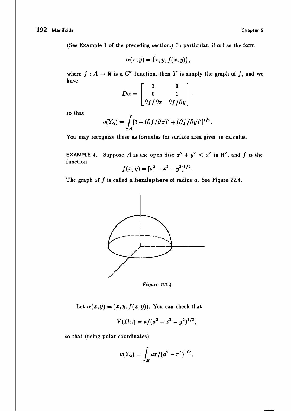
192 Manifolds Chapter 5
(See Example 1 of the preceding section.) In particular, if a has the form
a(x , y) = (x , y , /(x, y)) ,
where f : A __. R is a cr function, then Y is simply the graph of /, and we have
Da =
so that
1 0
of fax
0 1
of fay
You may recognize these as formulas for surface area given in calculus.
EXAMPLE 4. Suppose A is the open disc x2 + y2 < a2 in R2 , and f is the function
The graph of f is called a hemisphere of radius a. See Figure 22.4.
I I I
---� ----- I -....... / ..... }-------1------//
Figure 22.4
Let a(x, y) = ( x , y, f(x, y)). You can check that
so that (using polar coordinates)
§22. The Volume of a Parametrized-Manifold 193
where B is the open set ( 0 , a) x ( 0, 27r) in the ( r, B)-plane. This is an improper integral, so we cannot use the Fubini theorem, which was proved only for the ordinary integral. Instead, we integrate over the set (0, an ) x (0, 27r) using the Fubini theorem, where 0 < an < a, and then we let an _. a. We have
v(Ya) = lim (-27ra)[(a2 - a�) 1 /2 - a] = 21ra2. n-oo
A different method for computing this area, one that avoids improper integrals, is given in §25.
EXERCIS ES
1 . Let A be open in Rk; let a : A _. Rn be of class cr; let Y = a(A). Suppose h : Rn _. Rn is an isometry; let Z = h(Y) and let {3 = h o a. Show that Ya and Zf3 have the same volume.
2. Let A be open in Rk ; let f : A _. R be of class Cr; let Y be the graph of f in Rk+l , parametrized by the function a : A _. Rk+1 given by a(x) = (x , f(x)) . Express v(Ya) as an integral.
3. Let A be open in Rk; let a : A -- Rn be of class Cr; let Y = a(A). The centroid c(Ya) of the parametrized-manifold Ya is the point of Rn whose i1h coordinate is given by the equation
c; (Ya ) = [1/v(Ya )] 1 1r; dV,
where 7r; : Rn --+ R is the i1h projection function.
(a) Find the centroid of the parametrized-curve
a(t) = (a cos t , a sin t) with O < t < ?r.
(b) Find the centroid of the hemisphere of radius a in R3• (See Example 4.)
*4. The following exercise gives a strong plausibility argument justifying our definition of volume. We consider only the case of a surface in R3 , but a similar result holds in general.
Given three points a, b, c in R3, let C be the matrix with columns b - a and c-a. The transformation h : R2 _. R3 given by h(x) = C·x +a carries O , e1 , e2 to a, b, c, respectively. The image Y under h of the set
A = { ( x, y) I x > 0 and y > 0 and x + y < 1} is called the (open) triangle in R3 with vertices a, b, c. See Figure 22.5. The area of the parametrized-surface Yh is one-half the area of the parallelopiped with edges b - a and c - a, as you can check.

194 Manifolds
- -
Chapter 5
- -7 -- / -- / /
/ /
- - - - -, I I I I I
Figure 22.5
b
a
Now let Q be a rectangle in R2 and let a : Q __. R3 ; suppose a extends to a map of class Cr defined in an open set containing Q. Let P be a partition of Q. Let R be a subrectangle determined by P, say
R = [a, a + h] x [b, b + k] . Consider the triangle tl.t (R) having vertices
a(a, b) , a(a + h , b) , and a(a + h, b + k) and the triangle tl.2(R) having vertices
a(a, b) , a(a, b + k), and a(a + h, b + k) . We consider these two triangles to be an approximation to the "curved rectangle" a( R). See Figure 22.6. We then define
A(P) = I.:: [v (tl.t (R)) + v (tl.2(R)) ] , R
where the sum extends over all subrectangles R determined by P. This number is the area of a polyhedral surface that approximates a(Q). Prove the following:
Theorem. Let Q be a rectangle in R2 and let a : A -+ R3 be a map of class cr defined in an open set containing Q. Given f > o, there is a 6 > 0 such that for every partition P of Q of mesh less than 6,
A(P) - i V(Da) < c

§22. The Volume of a Parametrized-Manifold 195
. . (a , b + k) .' (a + h, b + k) I
lY' J (a, b) (a + h, b)
Q
Figure 22. 6
Proof. (a) Given points x1 , . . . , X6 of Q, let
D1at (x. ) D2at (x4 ) Va(xt , . . . , X6) = D1a2(x2 ) D2a2 (xs)
D1a3(x3 ) D2a3(x6 )
Then Va is just the matrix Da with its entries evaluated at different points of Q. Show that if R is a subrectangle determined by P, then there are points XI , . . . , x6 of R such that
v(6t (R)) = � V(Va(xt , . . . , x6 )) · v(R).
Prove a similar result for v ( 62 ( R)) . (b) Given f > 0, show one can choose 6 > 0 so that if Xi , y; E Q with
lx; - Yd < 6 for i = 1 , . . . , 6 , then
(c) Prove the theorem.
6t (R)
a(Q)

196 Manifolds Chapter 5
§23. MANI FOLDS IN Rn
Manifolds form one of the most important classes of spaces in mathematics . They are useful in such diverse fields as differential geometry, theoretical physics, and algebraic topology. We shall restrict ourselves in this book to manifolds that are sub manifolds of euclidean space Rn . In a final chapter, we define abstract manifolds and discuss how our results generalize to that case.
We begin by defining a particular kind of manifold .
Definition. Let k > 0. Suppose that M is a subspace of Rn having the following property: For each p E M, there is a set V containing p that is open in M, a set U that is open in Rk , and a continuous map a : U -+ V carrying U onto V in a one-to-one fashion, such that:
( 1) a is of class cr . (2) a-1 : V -+ U is continuous.
(3) Da(x) has rank k for each x E U . Then M is called a k-manifold without boundary i n Rn , of class cr . The map a is called a coordinate patch on M about p.
Let us explore the geometric meaning of the various conditions in this definition .
EXAMPLE 1 . Consider the case k = 1 . If a is a coordinate patch on M, the condition that Da have rank 1 means merely that Da :f. 0. This condition rules out the possibility that 1\{ could have "cusps" and "corners." For example, let a : R -+ R2 be given by the equation a(t) = (t3 , e), and let M be the image set of a. Then M has a cusp at the origin. (See Figure 23.1 .) Here a is of class c= and a-1 is continuous, but Da does not have rank 1 at t = o.
Figure 23. 1
Similarly, let {3 : R -+ R2 be given by {3(t) = W, WI ), and let N be the image set of (3. Then N bas a corner at the origin. (See Figure 23.2.) Here

§23. Manifolds in Rn 197
j3
Figure 23.2
j3 is of class C2 (as you can check) and {3-1 is continuous , but Dj3 does not have rank 1 at t = 0.
EXAMPLE 2. Consider the case k = 2. The condition that Da(a) have rank 2 means that the columns oaf OXI and oaf OX2 of Da are independent at a. Note that oafoxi is the velocity vector of the curve f(t) = a(a + tei ) and is thus tangent to the surface M. Then oafoxl and 8ajox2 span a 2-dimensional "tangent plane" to M. See Figure 23.3.
M
Figure 23.3
As an example of what can happen when this condition fails, consider the function a : R2 -+ R3 given by the equation
and let M be the image set of a. Then M fails to have a tangent plane at the origin. See Figure 23.4. The map a is of class Coo and a-1 is continuous, but Da does not have rank 2 at 0.

198 Manifolds Chapter 5
( 0
M
Figure 23.4
EXAMPLE 3. The condition that a-1 be continuous also rules out vanous sorts of "pathological behavior." For instance, let a be the map
a(t) = (sin 2t) ( I cos t I , sin t) for 0 < t < 1r,
and let M be the image set of a. Then M is a "figure eight" in the plane. The map a is of class C1 with Da of rank 1 , and a maps the interval (0, 1r) in a one-to-one fashion onto M. But the function a-1 is not continuous. For continuity of a-1 means that a carries any set Uo that is open in U onto a set that is open in M. In this case, the image of the smaller interval Uo pictured in Figure 23.5 is not open in M. Another way of seeing that a-1 is not continuous is to note that points near 0 in M need not map under a-1 to points near 1r /2.
a ...........---
Uo M
( • ) ) ?r/2 1r
Figure 23.5
EXAMPLE 4. Let A be open in Rk ; let a : A -+ Rn be of class Cr; let Y = a(A). Then Ya is a parametrized-manifold; but Y need not be a manifold. However, if a is one-to-one and a-1 is continuous and Da has rank k,

Manifolds in Rn 199
then Y is a manifold without boundary, and in fact Y is covered by the single coordinate patch a.
Now we define what we mean by a manifold in general . We must first generalize our notion of differentiability to functions that are defined on arbitrary subsets of Rk .
Definition. Let S be a subset of Rk ; let J : S --+ Rn. We say that J is of class cr on S if f may be extended to a function g : U --+ Rn that is of class cr on an open set U of Rk containing S.
It follows from this definition that a composite of cr functions is of class Cr . Suppose S C Rk and /I : S --+ Rn is of class Cr . Next, suppose that T c Rn and /I (S) c T and 12 : T --+ RP is of class cr . Then /2 o/J : s --+ RP is of class cr . For if YI is a cr extension of !I to an open set u in Rk ' and if Y2 is a cr extension of /2 to an open set v in Rn ' then Y2 0 YI is a cr extension of /2 o /I that is defined on the open set YII (V) of Rk containing S.
The fol lowing lemma shows that f is of class cr if it is locally of class cr:
Lemma 23.1. Let S be a subset of Rk; let f : S --+ Rn. If for each x E S, there is a neighborhood Ux of x and a function Yx : Ux -> Rn of class cr that agrees with J on Ux n S, then J is of class cr on S.
Proof. The lemma was given as an exercise in §16 ; we provide a proof here. Cover S by the neighborhoods Ux; let A be the union of these neighborhoods ; let { ¢>;} be a partition of unity on A of class cr dominated by the collection {Ux} · For each i , choose one of the neighborhoods Ux containing the support of ¢>; , and let g; denote the Cr function Yx : Ux --+ Rn . The Cr function </>;g; : Ux --+ Rn vanishes outside a closed subset of Ux ; we extend it to a cr function h; on all of A by letting it vanish outside Ux . Then we define
00
g(x) = L h;(x) i=I
for each x E A . Each point of A has a neighborhood on which g equals a finite sum of functions h; ; thus g is of class cr on this neighborhood and hence on all of A. Furthermore, if x E S, then
h;(x) = </>;(x)g; (x) = </>; (x)f(x)
for each i for which ¢>;(x) :f 0. Hence if x E S, 00
g(x) = L </>;(x)f(x) = /(x) . 0 i=I

200 Manifolds Chapter 5
Definition. Let Hk denote upper half-space in Rk , consisting of those x E Rk for which xk > 0. Let Hi denote the open upper half-space, consisting of those x for which Xk > 0.
We shall be particularly interested in functions defined on sets that are open in Hk but not open in Rk . In this situation , we have the fol lowing useful result:
Lemma 23.2. Let U be open in Hk but not in Rk ; let a : U -+ R" be of class cr . Let j3 : U' -+ Rn be a cr extension of a defined on an open set U' of Rk . Then for x E U , the derivative Dj3(x) depends only on the function a and is independent of the extension {3. It follows that we may denote this derivative by Da (x) without ambiguity.
Proof. Note that to calculate the partial derivative 8{31f8x1 at x, we form the difference quotient
[/3(x + hei ) - /3(x)] / h
and take the limit as h approaches 0. For calculation purposes, it suffices to let h approach 0 through positive values. In that case, if x is in Hk then so is x + hei . Since the functions j3 and a agree at points of Hk , the value of Dj3(x) depends only on a. See Figure 23.6. D
Figure 23.6
Now we define what we mean by a manifold.
I I \ \
' ' ....... ...... _ _ _...
Definition. Let k > 0. A k-manifold in Rn of class cr is a subspace M of Rn having the following property: For each p E M, there is an open

Manifolds in R" 201
set V of M containing p, a set U that is open in either Rk or Hk , and a continuous map a : U -+ V carrying U onto V in a one-to-one fashion, such that:
(1) a is of class cr . (2) a- 1 : V -+ U is continuous. (3) Da(x) has rank k for each x E U.
The map a is called a coordinate patch on M about p.
We extend the definition to the case k = 0 by declaring a discrete collection of points in R" to be a 0-manifold in R".
Note that a manifold without boundary is simply the special case of a manifold where all the coordinate patches have domains that are open in Rk .
Figure 23.7 illustrates a 2-manifold in R3. Indicated are two coordinate patches on M, one whose domain is open in R2 and the other whose domain is open in H2 but not in R2 .
Figure 23. 7
It seems clear from this figure that in a k-manifold , there are two kinds of points, those that have neighborhoods that look like open k-balls, and those that do not but instead have neighborhoods that look like open half-balls of dimension k. The latter points constitute what we shall call the boundary of M. Making this definition precise, however, requires a certain amount of effort. We shall deal with this question in the next section.
We close this section with the fol lowing elementary result:

202 Manifolds Chapter 5
Lemma 23.3. Let M be a manifold in R", and let a : U -+ V be a coordinate patch on M. If U0 is a subset of U that is open in U, then the restriction of a to Uo is also a coordinate patch on M.
Proof. The fact that U0 is open in U and a-1 is continuous implies that the set V0 = a( Uo ) is open in V. Then U0 is open in Rk or Hk (according as U is open in Rk or Hk ) , and V0 is open in M. Then the map aJU0 is a coordinate patch on M: it carries Uo onto V0 in a one-to-one fashion; it is of class cr because a is; its inverse is continuous being simply a restriction of a-1 ; and its derivative has rank k because Da does. 0
Note that this result would not hold if we had not required a-1 to be continuous. The map a of Example 3 satisfies all the other conditions for a coordinate patch, but the restricted map a JU0 is not a coordinate patch on M, because its image is not open in !11.
EXERCISES
1 . Let a : R -+ R2 be the map a(x) = (x , x2) ; let M be the image set of a. Show that M is a 1-manifold in R2 covered by the single coordinate patch a.
2. Let {3 : W -+ R2 be the map {J(x) = (x, x2 ) ; let N be the image set of {3. Show that N is a 1-manifold in R2 .
3. (a) Show that the unit circle S1 is a 1-manifold in R2 .
(b) Show that the function a : [o, 1 ) -+ S1 given by
a(t) = (cos 21rt, sin 21rt) is not a coordinate patch on S1 •
4 . Let A be open in Rk; let f : A --+ R be of class cr . Show that the graph of j is a k-manifold in Rk+I .
5. Show that if M is a k-manifold without boundary in Rm, and if N is an £-manifold in R"' then M X N is a k + l manifold in nm+ n .
6. (a) Show that I = [0, 1] is a 1-manifold in R1 .
(b) Is I x I a 2-manifold in R2? Justify your answer.

§24. The Boundary of a Manifold 203
§24. THE BOUN DARY OF A MANIFOLD
In this section, we make precise what we mean by the boundary of a manifold; and we prove a theorem that is useful in practice for constructing manifolds.
To begin , we derive an important property of coordinate patches, namely, the fact that they "overlap differentiably." We make this statement more precise as fol lows:
Theorem 24.1 . Let M be a k-manifold in Rn , of class cr . Let a0 : U0 --+ V0 and a1 : U1 --+ V1 be coordinate patches on M, with W = V0 n Vi non-empty. Let W; = a;-1 (W) . Then the map
a1 1 o ao : Wo --+ W1 is of class cr ' and its derivative is non-singular.
Typical cases are pictured in Figure 24. 1. We often call a1 1 o ao the transition function between the coordinate patches a0 and a1 •
Figure 24 .1
Proof It suffices to show that if a : U --+ V is a coordinate patch on M, then a- 1 : V --+ Rk is of class cr , as a map of the subset V of Rn into Rk . For

204 Manifolds Chapter 5
then it follows that, since ao and a11 are of class cr , so is their composite a1 1 o a0. The same argument applies to show a0 1 o a1 is of class Cr ; then the chain rule implies that both these transition functions have non-singular derivatives.
To prove that a- 1 is of class cr , it suffices (by Lemma 23.1) to show that it is locally of class cr . Let Po be a point of V; let a-1 (Po) = Xo . We show a-1 extends to a cr function defined in a neighborhood of p0 in R".
Let us first consider the case where U is open in Hk but not in Rk . By assumption , we can extend a to a cr map {3 of an open set U' of Rk into R". Now Da(x0) has rank k, so some k rows of this matrix are independent; assume for convenience the first k rows are independent. Let 1r : R" --+ Rk project R" onto its first k coordinates. Then the map g = 1r o {3 maps U' into Rk , and Dg(x0) is non-singular. By the inverse function theorem, g is a cr diffeomorphism of an open set W of Rk about x0 with an open set in Rk . See Figure 24.2.
M
u
J - g
'?r w
U' <9g(W) Figure 24 .2
We show that the map h = g- 1 o 1r , which is of class Cr , is the desired extension of a- 1 to a neighborhood A of p0. To begin, note that the set U0 = W n U is open in U, so that the set V0 = a(Uo) is open in V; this

§24. The Boundary of a Manifold 205
means there is an open set A of R" such that A n V = Vo . We can choose A so it is contained in the domain of h (by intersecting with 1r- 1 (g(W)) if necessary) . Then h : A -+ Rk is of class Cr ; and if p E A n V = V0 , then we let x = a- 1 (p) and compute
h(p) = h (a(x)) = g- 1 (1r(a(x))) = g- 1 (g(x)) = x = a-1 (p),
as desired. A similar argument holds if U is open in Rk . In this case, we set U' = U
and {3 = a, and the preceding argument proceeds unchanged. 0
Now we define the boundary of a manifold.
Definition. Let M be a k-manifold in R"; let p E M. If there is a coordinate patch a : U -+ V on M about p such that U is open in Rk , we say p is an interior point of M . Otherwise , we say p is a boundary point of M. We denote the set of boundary points of M by oM , and call this set the boundary of M .
Note that our use here of the terms "interior" and "boundary" has nothing to do with the way these terms are used in general topology. Any subset S of R" has an interior and a boundary and an exterior in the topological sense, which we denote by Int S and Bd S and Ext S, respectively. For a manifold M, we denote its boundary by oM and its interior by M - oM.
Given M, one can readily identify the boundary points of M by use of the fol lowing criterion:
Lemma 24.2. Let M be a k-manifold in R" ; let a : U -+ V be a coordinate patch about the point p of M .
(a) If U is open in Rk , then p is an interior point of M.
(b) If U is open in Hk and if p = a(xo ) for xo E Hi, then p is an interior point of M.
(c) If U is open in Hk and p = a(xo) for x0 E Rk- I x 0, then p is a boundary point of M.
Proof (a) is immediate from the definition. (b) is almost as easy. Given a : U -+ V as in (b) , let Uo = U n Hi and let Vo = a(Uo) . Then a iUo, mapping Uo onto V0, is a coordinate patch about p, with Uo open in Rk .
We prove (c) . Let a0 : U0 -+ V0 be a coordinate patch about p, with Uo open in Hk and p = ao(xo) for xo E Rk- I x 0. We assume there is a coordinate patch a1 : U1 -+ V1 about p with U1 open in Rk . and derive a contradiction .

206 Manifolds Chapter 5
Since V0 and V1 are open in M, the set W = Vo n V1 is also open in M.
Let W; = a;1 (W) for i = 0 , 1 ; then Wo is open in Hk and contains x0 , and W1 is open in Rk . The preceding theorem tells us that the transition function
is a map of class cr carrying W1 onto W0 in a one-to-one fashion, with non-singular derivative. Then Theorem 8.2 tells us that the image set of this map is open in Rk . But W0 is contained in Hk and contains the point x0 of Rk- l x 0, so it is not open in Rk ! See Figure 24.3. 0
Wo
xo
Wt (?)
• Figure 24 .3
Note that Hk is itself a k-manifold in Rk ; and it fol lows from this lemma that oHk = Rk-I x 0 .
Theorem 24.3. Let M be a k-manifold in Rn, of class Cr . If oM is non-empty, then oM is a k - 1 manifold without boundary in Rn of class cr .
Proof. Let p E 0 M. Let a : U -+ V be a coordinate patch on M
about p. Then U is open in Hk and p = a(xo ) for some x0 E oHk . By the preceding lemma, each point of U n Hi is mapped by a to an interior point of M, and each point of U n (oHk ) is mapped to a point of oM. Thus the

§24. The Boundary of a Manifold 207
restriction of a to U n (oHk ) carries this set in a one-to-one fashion onto the open set V0 = V n oM of oM . Let U0 be the open set of Rk- I such that Uo x 0 = U n 8Hk ; if x E U0 , define ao (x) = a(x, 0). Then ao : Uo -+ Vo is a coordinate patch on oM. It is of class cr because a is, and its derivative has rank k - 1 because Da0(x) consists simply of the first k - 1 columns of the matrix Da(x, 0). The inverse a0 1 is continuous because it equals the restriction to V0 of the continuous function a-1 , followed by projection of Rl: onto its first k - 1 coordinates. 0
The coordinate patch ao on oM constructed in the proof of this theorem is said to be obtained by restricting the coordinate patch a on M.
Finally, we prove a theorem that is useful in practice for constructing manifolds.
Theorem 24.4. Let 0 be open in R" ; let f : 0 -+ R be of class cr . Let M be the set of points x for which f(x) = 0; let N be the set of points for which f(x) > 0. Suppose M is non-empty and D f(x) has rank 1 at each point of M. Then N is an n-manifold in R" and oN = M.
Proof. Suppose first that p is a point of N such that f (p) > 0 . Let U be the open set in R" consisting of all points x for which f(x) > 0; let a : U -+ U be the identity map. Then a is (trivially) a coordinate patch on N about p whose domain is open in R".
Now suppose that /(p) = 0. Since D f(p) is non-zero, at least one of the partial derivatives D;f(p) is non-zero. Suppose Dnf(p) :f 0. Define F : 0 -+ R" by the equation F(x) = (x. , . . . , Xn -1 ! /(x)) . Then [ ln-1 DF =
*
so that DF(p) is non-singular. It follows that F is a diffeomorphism of a neighborhood A of p in R" with an open set B of R". Furthermore, F carries the open set A n N of N onto the open set B n H" of H", since x E N if and only if /(x) > 0 . It also carries A n M onto B n oH", since x E M if and only if f(x) = 0. Then F- 1 : B n H" -+ A n N is the required coordinate patch on N. See Figure 24.4. 0
Definition. Let B"(a) consist of all points x of R" for which l lxl l < a , and let S"-1 (a) consist of all X for which l lxl l = a . We call them the n-ball and the n - 1 sphere, respectively, of radius a .
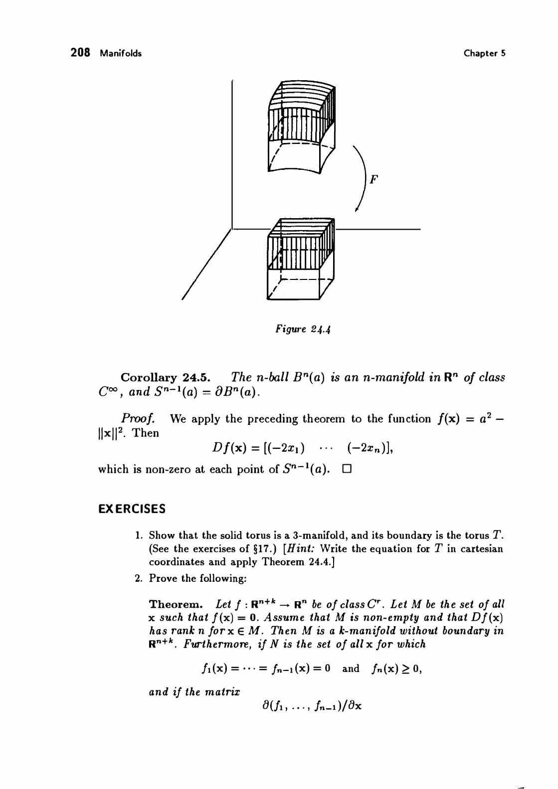
208 Manifolds Chapter 5
F
Figure 24.4
Corollary 24.5. The n-ball B"(a) is an n-manifold in R" of class coo , and S"- 1 (a) = 8B" (a) .
Proof. We apply the preceding theorem to the function f(x) = a2 -l lxW. Then
Df(x) = [(-2xi ) · · · (-2xn )] ,
which is non-zero at each point of S"- 1 (a). 0
EX ERCISES
1 . Show that the solid torus is a 3-manifold, and its boundary is the torus T. (See the exercises of §17 . ) [Hint: Write the equation for T in cartesian coordinates and apply Theorem 24.4.]
2. Prove the following:
Theorem. Let f : nn+k _,. Rn be of class cr . Let M be th e set of all x such that f (x) = 0. Assume that M is non-empty and that D f(x) has rank n for x E M. Then M is a k-manifold without boundary in nn+k . Furthermore, if N is the set of all X for which
ft (x) = . . · = fn-I (x) = 0 and fn (x) > 0,
and if the matrix 0(/1 , . . · , fn-1 )/OX

§25. Integrating a Scalar Function over a Manifold 209
has rank n - 1 at each point of N, then N is a k + 1 manifold, and oN = M.
3. Let f, g : R3 __. R be of class Cr. Under what conditions can you be sure that the solution set of the system of equations f(x , y, z ) = 0, g(x, y, z) = 0 is a smooth curve without singularities (i .e., a !-manifold without boundary)?
4 . Show that the upper hemisphere of sn-l (a) , defined by the equation
is an n - 1 manifold. What is its boundary?
5. Let 0(3) denote the set of all orthogonal 3 by 3 matrices, considered as a subspace of R9.
(a) Define a coo function f : R9 __. R6 such that 0(3) is the solution set of the equation f(x) = 0.
(b) Show that 0(3) is a compact 3-manifold in R9 without boundary. [Hint: Show the rows of Df (x) are independent if x E 0(3).]
6. Let 0( n) denote the set of all orthogonal n by n matrices, considered as a subspace of RN, where N = n2 • Show 0( n) is a compact manifold without boundary. What is its dimension?
The manifold 0( n) is a particular example of what is called a Lie group (pronounced "lee group" ). It is a group under the operation of matrix multiplication; it is a coo manifold; and the product operation and the map A __. A-! are coo maps. Lie groups are of increasing importance in theoretical physics, as well as in mathematics.
§25 . INTEGRATING A SCALAR FUNCTION OVER A MANIFOLD
Now we define what we mean by the integral of a continuous scalar function f over a manifold M in R" . For simplicity, we shall restrict ourselves to the case where M is compact. The extension to the general case can be carried out by methods analogous to those used in §16 in treating the extended integral.
First we define the integral in the case where the support of f can be covered by a single coordinate patch.
Definition. Let M be a compact k-manifold in R", of class cr . Let f : M --+ R" be a continuous function. Let C = Support / ; then C is compact. Suppose there is a coordinate patch a : U -+ V on M such that C C V. Now a- 1 (C) is compact. Therefore, by replacing U by a smaller open

210 Manifolds Chapter 5
set if necessary, we can assume that U is bounded. We define the integral of f over M by the equation
f f dV = 1. (f o a)V(Da) . jM Int U
Here Int U = U if U is open in Rk , and Int U = U n Hi if U is open in Hk but not in Rk .
It is easy to see this integral exists as an ordinary integral , and hence as an extended integral : The function F = (f o a)V(Da) is continuous on U and vanishes outside the compact set a- 1 (C); hence F is bounded. If U is open in Rk , then F vanishes near each point x0 of Bd U. If U is not open in Rk , then F vanishes near each point of Bd U not in 8Hk , a set that has measure zero in Rk . In either case, F is integrable over U and hence over Int U. See Figure 25 .1 .
u
Figure 25.1
Lemma 25.1. If the support off can be covered by a single coordinate patch, the integral JM f dV is well-defined, independent of the choice of coordinate patch.

§25. Integrating a Scalar Function over a Manifold 211
Proof. We prove a preliminary result. Let a : U -+ V be a coordinate patch containing the support of f. Let W be an open set in U such that a(W) also contains the support of f. Then
f (f o a)V(Da) = f (f o a)V(Da); lint W lint U
the (ordinary) integrals over W and V are equal because the integrand vanishes outside W; then one applies Theorem 13.6.
Let a; : U; -+ V; for i = 0, 1 be coordinate patches on M such that both V0 and Vi contain the support of f. We wish to show that
f (f o a0)V(Da0 ) = 1 (f o ai )V(Dat ) . lint Uo Int U1
Let W = V0nV1 and let W; = a; 1 (W ) . In view of the result of the preceding paragraph, it suffices to show that this equation holds with U; replaced by W; , for i = 0, 1 . Since a1 1 o a0 : Int W0 -+ Int W1 is a diffeomorphism, this result follows at once from Theorem 22. 1 . 0
To define JM f dV in general, we use a partition of unity on M.
Lemma 25.2. Let M be a compact k-manifold in R", of class Cr . Given a covering of M by coordinate patches, there exists a finite collection of coo functions ¢1 , . . . , <Pt mapping R" into R such that:
( 1 ) ¢; (x) > 0 for all x.
(2) Given i, the support of ¢; is compact and there is a coordinate patch a; : U; -+ V; belonging to the given covering such that
((Support ¢; ) n M) c V;.
(3) L: ¢; (x) = 1 for x E M.
We call { ¢1 , . . • , ¢t } a partition of unity on M dominated by the given collection of coordinate patches.
Proof. For each coordinate patch a : U -+ V belonging to the given collection , choose an open set Av of R" such that Av n M = V. Let A be the union of the sets Av . Choose a partition of unity on A that is dominated by this open covering of A. Local finiteness guarantees that all but finitely many of the functions in the partition of unity vanish identically on M. Let ¢1 , • • • , <Pt be those that do not. 0
Definition. Let M be a compact k-manifold in R", of class cr . Let f : M -+ R be a continuous function. Choose a partition of unity ¢1 , • • . , <Pt
212 Manifolds Chapter 5
on M that is dominated by the collection of all coordinate patches on M. We define the integral of f over M by the equation
l 1 t dV = I:r1 (¢d) dVJ. M i=l M Then we define the (k-dimensional) volume of M by the equation
v(M) = i 1 dV.
If the support of f happens to lie in a single coordinate patch a : U -+ V, this definition agrees with the preceding definition. For in that case, letting A = Int U, we have
l l L [1 (¢;/) dV) = L [1 (¢; o a)(f o a)V(Da)] by definition, i:l M i=l A
l = 1 [L (¢; o a)(f o a)V(Da)] by linearity,
A i=l
= L (f o a)V(Da) because
= jM J dV by definition.
l L (¢; o a) = 1 on A, i=l
We note also that this definition is independent of the choice of the partition of unity. Let 'I/J1 , • • • , '1/Jm be another choice for the partition of unity. Because the support of '1/Ji f lies in a single coordinate patch, we can apply the computation just given (replacing f by '1/Ji/) to conclude that
l I: r1 (¢;'1/Ji f) dVJ = 1 ('1/Ji /) dv. i=l M M
Summing over j , we have m l m I: I: r1 (¢;'1/Ji f) dVJ = I: r1 ('1/Ji /) dVJ .
i= l i=l M i= l M Symmetry shows that this double summation also equals
l I: r1 (¢d) dVJ , i:l M
as desired. Linearity of the integral follows at once. We state it formally as a theorem:

§25. Integrating a Scalar Function over a Manifold 213
Theorem 25.3. Let M be a compact k-manifold in R" , of class cr . Let J, g : M -+ R be continuous. Then
L (af + bg) dV a i t dV + b L g dV. 0
This definition of the integral JM f dV is satisfactory for theoretical purposes, but not for practical purposes. If one wishes actually to integrate a function over the n - 1 sphere sn- 1 , for example, what one does is to break sn- 1 into suitable "pieces," integrate over each piece separately, and add the results together. We now prove a theorem that makes this procedure more precise. We shall use this result in some examples and exercises .
Definition. Let M be a compact k-manifold in R", of class cr . A subset D of M is said to have measure zero in M if it can be covered by countably many coordinate patches a; : U; -+ V; such that the set
D; = a-1 (D n Vi)
has measure zero in Rk for each i. An equivalent definition is to require that for any coordinate patch
a : U -+ V on M, the set a- 1 ( D n V) have measure zero in Rk . To verify this fact, it suffices to show that a-1 (D n V n V;) has measure zero for each i . And this follows from the fact that the set ai 1 (D n V n V;) has measure zero because it is a subset of D;, and that a-1 o a; is of class cr .
*Theorem 25.4. Let M be a compact k-manifold in R", of class cr . Let f : M -+ R be a continuous function. Suppose that a; : A; -+ M; , for i = 1 , . . . , N, is a coordinate patch on M, such that A; is open in Rk and M is the disjoint union of the open sets M1 , . . . , MN of M and a set I< of measure zero in M. Then
N 1 f dV = L r1 (f 0 a;)V(Da;)] . M i=l A ; This theorem says that JM f dV can be evaluated by breaking M up
into pieces that are parametrized-manifolds and integrating f over each piece separately.
Proof. Since both sides of ( *) are linear in f, it suffices to prove the theorem in the case where the set C = Support f is covered by a single coordinate patch a : U -+ V. We can assume that U is bounded. Then
f f dV = f (f o a)V(Da), JM Jint U
by definition.

214 Manifolds Chapter 5
Step 1 . Let W; = a-1 (M; n V) and let L = a- 1 (K n V). Then W; is open in Rk , and L has measure zero in Rk ; and U is the disjoint union of L and the sets W; . See Figures 25.2 and 25.3. We show first that
Figure 25.2
Figure 25.3
Note that these integrals over W; exist as ordinary integrals . For the function F = (f o a)V(Da) is bounded , and F vanishes near each point of

§25. Integrating a Scalar Function over a Manifold 2 15
Bd W; not in L. Then we note that
L [ [ F] = [ F ; lw; j(Int U)-L
- f F Jlnt U
by additivity,
since L has measure zero,
by definition .
Step 2. We complete the proof by showing that
f F = f F; , lw; JA ; where F; = (f o a;)V(Da; ) . See Figure 25.4 .
I I
I I \ \ \
/ / / .,. .....
...... - - - - - -
I I
I
I r --
I -I ,.,. --1.-..,.. .....
', _ ..... .... ...... _ ....
-- -
- -- - -
W;
Figure 25.4
The map a; 1 o a is a diffeomorphism carrying W; onto the open set

216 Manifolds
of Rk . It follows from the change of variables theorem that
just as in Theorem 22. 1 . To complete the proof, we show that
f F; = f F; . jB; jA;
Chapter 5
These integrals may not be ordinary integrals, so some care is required . Since C = Support f is closed in M, the set aj1 (C) is closed in A; and
its complement D; = A; - aj 1 (C)
is open in A; and thus in Rk . The function F; vanishes on D;. We apply additivity of the extended integral to conclude that
f F; = f F; + f F; - f F; . jA; JB, lv, jB;nD, The last two integrals vanish. 0
EXAMPLE 1 . Consider the 2-sphere S2(a) of radius a in R3 . We computed the area of its open upper hemisphere as 27m2 • (See Example 4 of §22.). Since the reflection map ( x , y, z) __. ( x , y , - z) is an isometry of R3 , the open lower hemisphere also has area 27m2• (See the exercises of §22.) Since the upper and lower hemispheres constitute all of the sphere except for a set of measure zero in the sphere, it follows that S2(a) has area 47ra2 • EXAMPLE 2 . Here is an alternate method for computing the area of the 2-sphere; it involves no improper integrals.
Given Zo E R with l zo l < a, the intersection of S2(a) with the plane z = Zo is the circle
This fact suggests that we parametrize S2(a) by the function a : A __. R3
given by the equation
where A is the set of all ( t , z) for which 0 < t < 211" and l z l < a. It is easy to check that a is a coordinate patch that covers all of S2 (a) except for a great-circle arc, which has measure zero in the sphere. See Figure 25.5. By

§25. Integrating a Scalar Function over a Manifold 2 17
the preceding theorem, we may use this coordinate patch to compute the area of S2 (a). We have
Da =
-(a2 - z2 )1 /2 sin t (a2 - z2) 1 /2 cos t
0
(- z cos t)/(a2 - z2 )1 12 ( -z sin t)/(a2 - z2) 1 /2
1
whence V(Da) = a , as you can check. Then v(S2(a)) = JA a = 47m2 .
z
0 211" t
Figure 25.5
EXERC ISES
1 . Check the computations made in Example 2. 2. Let a(t) , ,B(t), J(t) be real-valued functions of class C1 on [0 , 1], with
f(t) > 0. Suppose M is a 2-manifold in R3 whose intersection with the plane z = t is the circle
if 0 < t < 1 , and is empty otherwise.
(a) Set up an integral for the area of M. [Hint: Proceed as in Example 2.]
(b) Evaluate when a and /3 are constant and f(t) = 1 + t2 . (c) What form does the integral take when f is constant and a(t) = 0
and {3(t) = at? (This integral cannot be evaluated in terms of the elementary functions.)
3. Consider the torus T of Exercise 7 of § 17.
(a) Find the area of this torus. [Hint: The cylindrical coordinate transformation carries a cylinder onto T. Parametrize the cylinder using the fact that its cross-section are circles.]

218 Manifolds Chapter 5
(b) Find the area of that portion of T satisfying the condition x2 + y'2 > b2 .
4. Let M be a compact k-manifold in Rn. Let h : Rn __. Rn be an isometry; let N = h(M). Let f : N __. R be a continuous function. Show that N is a k-manifold in Rn, and
Conclude that M and N have the same volume.
5. (a) Express the volume of Sn(a) in terms of the volume of Bn-1 (a). [Hint: Follow the pattern of Example 2.]
(b) Show that for t > 0,
[Hint: Use the result of Exercise 6 of § 19.]
6. The centroid of a compact manifold M in Rn is defined by a formula like that given in Exercise 3 of §22. Show that if M is symmetric with respect to the subspace X; = 0 of Rn, then c; (M) = 0.
*7. Let E�(a) denote the intersection of Sn(a) with upper half-space Hn+t . Let An = v (Bn(l )) . (a) Find the centroid of E� (a) in terms of An and An-1 · (b) Find the centroid of E� (a) in terms of the centroid of B�-1 (a). (See
the exercises of §19.)
8. Let M and N be compact manifolds without boundary in Rm and Rn, respectively.
(a) Let f : M __. R and g : N __. R be continuous. Show that
f f · g dV = [ f f dV] [ f g dV] . lMxN JM JN [Hint: Consider the case where the supports of f and g are contained in coordinate patches.]
(b) Show that v(M x N) = v(M) · v(N). (c) Find the area of the 2-manifold S1 X S1 in R4 .

Differential Forms
We have treated, with considerable generality, two of the major topics of multivariable calculus-differentiation and integration. We now turn to the third topic. It is commonly called "vector integral calculus," and its major theorems bear the names of Green, Gauss, and Stokes. In calculus, one limits oneself to curves and surfaces in W. We shall deal more generally with k
manifolds in Rn. In dealing with this general situation, one finds that the concepts of linear algebra and vector calculus are no longer adequate. One needs to introduce concepts that are more sophisticated; they constitute a subject called multilinear algebra that is a sequ el to linear algebra.
In the first three sections of this chapter, we introduce this subject; in these sections we use only the material on linear algebra treated in Chapter 1 . In the remainder of the chapter, we combine the notions of multilinear algebra with results about differentiation from Chapter 2 to define and study differential forms in Rn. Differential forms and their operators are what are used to replace vector and scalar fields and their operators-grad, curl, and div-when one passes from R3 to Rn.
In the succeeding chapter, additional topics , including integration, manifolds, and the change of variables theorem, will be brought into the picture, in order to treat the generalized version of Stokes' theorem in R".
219
220 Differential Forms Chapter 6
§26. M U LTILI N EAR ALG EBRA
Tensors
Definition. Let V be a vector space. Let Vk = V x · · · x V denote the set of all k-tuples (v1 , . . . , vk ) of vectors of V. A function f : Vk -+ R is said to be linear in the ith variable if, given fixed vectors Vj for j "I i, the function T : V -+ R defined by
is linear. The function f is said to be multilinear if it is linear in the ith variable for each i. Such a function f is also called a k-tensor, or a tensor of order k, on V . We denote the set of all k-tensors on V by the symbol .Ck(V). If k = 1, then .C1(V) is just the set of all linear transformations f : V -+ R . It is sometimes called the dual space of V and denoted by V* .
How this notion of tensor relates to the tensors used by physicists and geometers remains to be seen.
Theorem 26. 1 . space if we define
The set of all k-tensors on V constitutes a vector
(f + g) (v. , . . . , Vk ) = f(v. , . . . , Vk ) + g(vi , . . . , vk ) , (cf)(v1 , . . . , vk) = c(f(v 1 , . . . , vk )) .
Proof. The proof is left as an exercise. The zero tensor is the function whose value is zero on every k-tuple of vectors . 0
Just as is the case with linear transformations, a multilinear transformation is entirely determined once one knows its values on basis elements . That we now prove.
Lemma 26.2. Let a1 , . . . , an be a basis for V. If f,g : Vk -+ R are k-tensors on V, and if
f (a;, , . . . , a;� ) = g( a;, , . . . , a;� ) for every k-tuple I = (i. , . . . , ik ) of integers from the set { 1 , . . . , n}, then f = g.
§26. Multilinear Algebra 221
Note that there is no requirement here that the integers i. , . . . , ik be distinct or arranged in any particular order.
Proof. Given an arbitrary k-tuple (v1 , . . . , vk ) of vectors of V, let us express each v; in terms of the given basis, writing
Then we compute
n
n v; = L C;jaj .
i= l
/(v1 , . . . , vk ) = L c1j , /(aj, , v2 , . . . , vk ) j ,=l n n
= L L CJj, C2j, /(aj, , aj, , v3 , . . . , vk) , j ,= l j,=l
and so on. Eventually we obtain the equation
The same computation holds for g . It follows that f and g agree on all k-tuples of vectors if they agree on all k-tuples of basis elements . 0
Just as a linear transformation from V to W can be defined by specifying its values arbitrarily on basis elements for V, a k-tensor on V can be defined by specifying its values arbitrarily on k-tuples of basis elements . That fact is a consequence of the next theorem.
Theorem 26.3. Let V be a vector space with basis a. , . . . , an . Let I = (i. , . . . , ik ) be a k-tuple of integers from the set { 1 , . . . , n} . There is a unique k-tensor <h on V such that, for every k-tuple J = (j1 , . . . , jk) from the set { 1 , . . . , n} ,
The tensors <h form a basis for .Ck(V).
if I "# J, if I = J.
The tensors <h are called the elementary k-tensors on V corresponding to the basis a. , . . . , an for V. Since they form a basis for .Ck (V) and since there are nk distinct k-tuples from the set { 1 , . . . , n} , the space .Ck (V) must

222 Differential Forms Chapter 6
have dimension nk . When k = 1 , the basis for V* formed by the elementary tensors ¢1 , . . . , ¢n is called the basis for V* dual to the given basis for V.
Proof. Uniqueness follows from the preceding lemma. We prove existence as follows: First, consider the case k = 1 . We know that we can determine a linear transformation ¢; : V -+ R by specifying its values arbitrarily on basis elements. So we can define ¢; by the equation
{ 0 if i 'I j, ¢; (aj ) =
1 'f · · 1 z = } ·
These then are the desired 1-tensors . In the case k > 1 , we define ¢I by the equation
It follows, from the facts that ( 1 ) each ¢; is linear and (2) multiplication is distributive, that ¢I is multilinear. One checks readily that it has the required value on ( ah , · · · , ai� ) .
We show that the tensors ¢I form a basis for .Ck(V). Given a k-tensor f on V, we show that it can be written uniquely as a linear combination of the tensors ¢I . For each k-tuple I = (i1 , . . . , ik), let d1 be the scalar defined by the equation
di = f(a; , , . . . , a;� ) .
Then consider the k-tensor
g = E dJ¢; , J
where the summation extends over all k-tuples J of integers from the set {1 , . . . , n} . The value of g on the k-tuple (a;, . . . , a;� ) equals d�, by (*) , and the value of f on this k-tuple equals the same thing by definition . Then the preceding lemma implies that f = g. Uniqueness of this representation of f follows from the preceding lemma. 0
It follows from this theorem that given scalars di for all /, there is exactly one k-tensor f such that /(a;, , . . . , a;� ) = di for all / . Thus a k-tensor may be defined by specifying its values arbitrarily on k-tuples of basis elements .

§26. Multilinear Algebra 223
EXAMPLE 1 . Consider the case V = Rn. Let e1 , . . . , en be the usual basis for Rn; let t/>t ' . . . ' t/>n be the dual basis for C1 (V). Then if X has components Xt , . . . , Xn, we have
¢;(x) = ¢(x1e1 + · · · + Xnen ) = X; .
Thus ¢; : Rn __. R equals projection onto the i1h coordinate. More generally, given I = (it , . . . , i,. ) , the elementary tensor t/>1 satisfies
the equation
Let us write X = [xt · · · x,.] , and let X;j denote the entry of X in row i and column j. Then Xj is the vector having components Xtj , . . . , Xnj · In this notation,
Thus t/>1 is just a monomial in the components of the vectors x1 , • • • , x,.; and the general k-tensor on Rn is a linear combination of such monomials.
It follows that the general 1-tensor on Rn is a function of the form
f(x) = d1 X1 + · · · + dnXn ,
for some scalars d; . The general 2-tensor on Rn has the form
n g(x, y) = L d;jXiYi ,
i,j= l
for some scalars dij . And so on.
The tensor product
Now we introduce a produ ct operation into the set of all tensors on V. The product of a k-tensor and an £-tensor will be a k + l tensor .
Definition. Let f be a k-tensor on V and let g be an £-tensor on V. We define a k + l tensor f 0 g on V by the equation
It is easy to check that the function f 0 g is multilinear; it is called the tensor product of f and g .
We list some of the properties of this product operation:

224 Differential Forms Chapter 6
Theorem 26.4. Let J, g, h be tensors on V. Then the following properties hold:
(1) {Associativity). / 0 (g 0 h) = (f 0 g) 0 h. (2) {Homogeneity). (cf) 0 g = c(f 0 g) = f 0 (cg) . (3) {Distributivity). Suppose f and g have the same order. Then:
(f + g) 0 h = f 0 h + g 0 h, h 0 (f + g) = h 0 f + h 0 g.
( 4) Given a basis a1 , . . . , an for V, the corresponding elementary tensors </>I satisfy the equation
where I = (i1 , . . . , ik ) ·
Note that no parentheses are needed in the expression for </>I given in (4) , since 0 is associative. Note also that nothing is said here about commutativity. The reason is obvious; it almost never holds.
Proof The proofs are straightforward. Associativity is proved, for instance, by noting that (if J, g, h have orders k, l , m, respectively)
(f 0 (g 0 h)) (v. , . . . , Vk+L+m ) = /(vi , . . . , vk ) · g(vk+I , . . . , Vk+L ) · h(vk+l+h . . . , vk+l+m ) •
The value of (f 0 g) 0 h on the given tuple is the same. D
The action of a linear transformation
Finally, we examine how tensors behave with respect to linear transformation of the underlying vector spaces.
Definition. Let T : V -+ W be a linear transformation. We define the dual transformation
(which goes in the opposite direction) as follows: If f is in .Ck(W) , and if v1 , . . . , Vk are vectors in V, then
(T* f)( vi , . . . , vk ) = / (T(vi ) , . . . , T(vk )) .
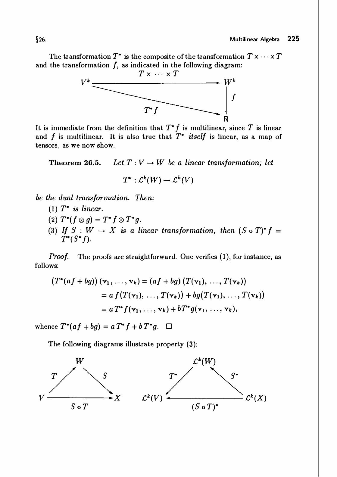
§26. Multilinear Algebra 225
The transformation T* is the composite of the transformation T x · · · x T and the transformation f, as indicated in the following diagram:
T X • • • X T yk ____________________________ Vfk
f T* f
R It is immediate from the definition that T* f is multilinear, since T is linear and f is multilinear. It is also true that T* itself is linear, as a map of tensors , as we now show.
Theorem 26.5. Let T : V -+ VV be a linear transformation; let
be the dual transformation. Then: (1) T* is linear. (2) T*(f 0 g) = T* f 0 T*g. (3) If S : VV -+ X is a linear transformation, then (S o T)* f =
T* (S* f) .
Proof. The proofs are straightforward. One verifies ( 1 ) , for instance, as follows:
(T* (af + bg)) (v1 , . . . , vk ) = (af + bg) (T(v. ) , . . . , T(vk )) = a f (T(v. ), . . . , T(vk )) + bg(T(v. ) , . . . , T(vk )) = a T* f ( v1 , . . . , vk ) + bT* g( v1 , . . . , vk ) ,
whence T*(af + bg) = a T* f + b T*g. 0
The following diagrams illustrate property (3):
T s T* s·
v ------ x .Ck(V) -------- .Ck (X) S o T (S o T)*
226 Differential Forms
EXERCISES
1. (a) Show that if /, g : Vk __. R are multilinear, so is af + bg. (b) Check that Ck ( V) satisfies the axioms of a vector space.
2. (a) Show that if f and g are multilinear, so is f ® g.
Chapter 6
(b) Check the basic properties of the tensor product (Theorem 26.4). 3 . Verify (2) and (3) of Theorem 26.5. 4. Determine which of the following are tensors on R4 , and express those
that are in terms of the elementary tensors on R4 :
/(x, y) = 3XtY2 + 5X2X3 ,
g(x , y) = X1Y2 + X2Y4 + 1 ,
h(x, y) = XtYt - 7X2Y3 ·
5. Repeat Exercise 4 for the functions
/(x, y, z) = 3XtX2Z3 - X3Y1 Z4 ,
h(x, y, z) = X1 Y2Z4 + 2XI Z3 .
6. Let f and g be the following tensors on R4 :
f(x, y , z) = 2XtY2Z2 - X2Y3Z1 ,
(a) Express f ® g as a linear combination of elementary 5-tensors.
(b) Express (f ® g) (x, y, z , u, v) as a function.
7. Show that the four properties stated in Theorem 26.4 characterize the tensor product uniquely, for finite-dimensional spaces V.
8. Let f be a 1-tensor on Rn; then /(y) = A · y for some matrix A of size 1 by n. If T : Rm __. Rn is the linear transformation T(x) = B · x, what is the matrix of the 1-tensor T* f on Rm?
§27. ALTERNATING TENSORS
In this section we introduce the particular kind of tensors with which we shall be concerned-the alternating tensors-and derive some of their properties. In order to do this, we need some basic facts about permutations.

§27. Alternating Tensors 227
Permutations
Definition. Let k > 2 . A permutation of the set of integers { 1 , . . . , k} is a one-to-one function a mapping this set onto itself. We denote the set of all such permutations by Sk . If a and T are elements of Sk , so are a o T and a-1 • The set Sk thus forms a group , called the symmetric group (or the permutation group) on the set { 1 , . . . , k} . There are k! elements in this group.
Definition. Given 1 < i < k, let e; be the element of Sk defined by setting e;(j) = j for j "I i, i + 1 ; and
e; (i) = i + 1 and e; (i + 1) = i .
We call e; an elementary permutation. Note that e; oe; equals the identity permutation, so that e; is its own inverse.
Lemma 27.1 . permutations.
If a E Sk , then a equals a composite of elementary
Proof. Given 0 < i < k, we say that a fixes the first i integers if a(j) = j for 1 < j < i. If i = 0, then a need not fix any integers at all. If i = k, then a fixes all the integers 1 , . . . , k, so that a is the identity permutation . In this case the theorem holds , since the identity permutation equals ei o ei for any j .
We show that if a fixes the first i-1 integers (where 0 < i < k) , then a can be written as the composite a = 1r o a', where 1r is a composite of elementary permutations and a' fixes the first i integers . The theorem then follows by induction.
The proof is easy. Since a fixes the integers 1 , . . . , i - 1 , and since a is one-to-one, the value of a on i must be a number different from 1 , . . . , i - 1 . If a(i) = i, then we set a' = a and 1r equal to the identity permutation , and our result holds. If a( i) = l > i, we set
I a = e; o · · · O el- l o a.
Then a' fixes the integers 1 , . . . , i - 1 because a fixes these integers and so do e; , . . . , el- l . And a' also fixes i, since a ( i) = l and
e; ( · · · ( et- 1 ( l)) · · · ) = i .
We can rewrite the equation defining a' in the form
thus our result holds. D
el- l o · · · o e; o a' = a;

228 Differential Forms Chapter 6
Definition. Let a E Sk . Consider the set of all pairs of integers i , j from the set { 1 , . . . , k} for which i < j and a (i) > a(j) . Each such pair is called an inversion in a . We define the sign of a to be the number -1 if the number of inversions in a is odd , and to be the number +1 if the number of inversions in a is even . We call a an odd or an even permutation according as the sign of a equals - 1 or +1 , respectively. Denote the sign of a by sgn a.
Lemma 27.2. Let a, T E Sk . (a) If a equals a composite of m elementary permutations, then
sgn a = (- 1)m . (b) sgn(a o r) = (sgn a) · (sgn r) . (c) sgn a- 1 = sgn a. (d) If p "I q, and if T is the permutation that exchanges p and q and
leaves all other integers fixed, then sgn T = - 1 .
Proof. Step 1. We show that for any a,
sgn(a o et) = -sgn a.
Given a, let us write down the values of a in order as follows:
(a(1 ) , a(2), . . . , a(l) , a(l + 1 ) , . . . , a(k)) .
Let T = aoel ; then the corresponding sequence for T is the k-tuple of numbers
(r( 1 ) , r(2), . . . , r(l) , r(l + 1) , . . . , r(k)) = (a( 1) , a( 2), . . . , a( l + 1) , a( l), . . . , a( k)) .
The number of inversions in a and T, respectively, are the number of pairs of integers that appear in the sequences ( *) and ( * * ) , respectively, in the reverse of their natural order. We compare inversions in these two sequences. Let p "I q; we compare the positions of a(p) and a(q) in these two sequences . If neither p nor q equals l or l + 1 , then a(p) and a( q) appear in the same slots in both sequences, so they constitute an inversion in one sequence if and only if they constitute an inversion in the other. Now consider the case where one, say p, equals either l or l + 1 , and the other q is different from both l and l + 1 . Then a (q) appears in the same slot in both sequences, but a(p) appears in the two sequences in adjacent slots. Nevertheless, it is still true that a(p) and a (q) constitute an inversion in one sequence if and only if they constitute an inversion in the other.
So far the number of inversions in the two sequences are the same. But now we note that if a( l) and a( l + 1 ) form an inversion in the first sequence, they do not form an inversion in the second ; and conversely. Hence sequence ( ** ) has either one more inversion , or one fewer inversion, than ( * ) .

§27. Alternating Tensors 229
Step 2. We prove the theorem. The identity permutation has sign +1 ; and composing it successively with m elementary permutation changes its sign m times , by Step 1 . Thus (a) holds. To prove (b), we write a as the composite of m elementary permutations , and T as the composite of n
elementary permutations. Then a o T is the composite of m + n elementary permutations; and (b) follows from the equation ( -1 )m+n = ( -1)m ( -1 )" . To check (c), we note that since a- I o a equals the identity permutation , (sgn a- I)(sgn a) = 1 .
To prove (d), one simply counts inversions. Suppose that p < q. We can write the values of T in order as
(1 ' . . . ' p - 1' [q] ' p + 1 ' . . . ' p + l - 1 ' !E] ' p + l + 1 ' . . . ' k),
where q = p+l. Each of the pairs {q, p+ 1} , . . . , {q, p+i- 1} constitutes an inversion in this sequence, and so does each of the pairs {p + 1 , p} . . . . , {p + l - 1 ,p} . Finally, {q, p} is an inversion as well. Thus T has 2l - 1 inversions, so it is odd . 0
Alternating tensors
Definition. Let f be an arbitrary k-tensor on V. If a is a permutation of { 1 , . . . ' k}, we define r by the equation
/17 (v. , . . . , vk) = f(va( I ) • . . . , Va(k)) ·
Because f is linear in each of its variables, so is /17 ; thus /17 is a k-tensor on V. The tensor f is said to be symmetric if fe = f for each elementary permutation e, and it is said to be alternating if r = -f for every elementary permutation e.
Said differently, f is symmetric if
for all i; and f is alternating if
/(vi , . . . , vi+ I , v;, . . . , vk) = -/(vi , . . . , v; , v;+ I , . . . , vk) ·
While symmetric tensors are important in mathematics, we shall not be concerned with them here. We shall be primarily interested in alternating tensors.
Definition. If V is a vector space, we denote the set of alternating ktensors on V by Ak (V). It is easy to check that the sum of two alternating tensors is alternating, and that so is a scalar multiple of an alternating tensor. Then Ak(V) is a linear subspace of the space .Ck(V) of all k-tensors on V. The condition that a 1-tensor be alternating is vacuous . Therefore we make the convention that AI (V) = .CI (V).

230 Differential Forms Chapter 6
EXAMPLE 1 . The elementary tensors of order k > 1 are not alternating, but certain linear combinations of them are alternating. For instance, the tensor
f = tPi,j - tPi,i
is alternating, as you can check. Indeed, if V = Rn and we use the usual basis for Rn and corresponding dual basis ¢;, the function f satisfies the equation [ X; Yi ]
f(x, y) = x ;yj - Xjy; = det . Xj Yi
Here it is obvious that /(y, x) = -f(x, y). Similarly, the function
x, Yi Z; g(x, y, z) = det x3 Yi Zj
is an alternating 3-tensor on Rn; one can also write g in the form
g = tPi,j,k + t/>j,k,i + tPk, i ,j - t/>j,i,k - tPi,k,j - tPk,j,i ·
This example suggests that alternating tensors and the determinant function are intimately related . This is in fact the case, as we shall see.
We now study the space Ak(V); in particular, we find a basis for it . Let us begin with a lemma:
Lemma 27.3. Let f be a k-tensor on V; let a, r E Sk . (a) The transformation f -+ j'I is a linear transformation of .Ck (V)
to .Ck (V). It has the property that for all a, r,
(J'IY = roa . (b) The tensor f is alternating if and only if j'I = (sgn a)f for all a .
Iff is alternating and if vp = vq with p "I q , then /(vi , . . . , vk) = 0.
Proof. (a) The linearity property is straightforward; it states simply that (af + bg)ti == aj'I + bga . To complete the proof of (a) , we compute
<rY (vl , . . . ' Vk) == r<vT( l ) , . . . ' VT(k) )
== f(wa( I ) • . . . , Wa(k) )
== /(vT(a( I )) • · · · , VT(a(k)) )
== fTOtJ(v. , . . . , vk) ·

Alternating Tensors 231
(b) Given an arbitrary permutation a, let us write it as the composite
where each a; is an elementary permutation. Then
= ( - 1 )m f because f is alternating,
= (sgn a)f. Now suppose vp = vq for p =I q. Let T be the permutation that ex
changes p and q. Since vp = vq ,
On the other hand,
r<v. , . . . ' vk ) = -f(v. , . . . , vk )
since sgn T = - 1. It follows that f(v. , . . . , vk) = 0. 0
We now obtain a basis for the space Ak(V). There is nothing to be done in the case k = 1 , since A1 (V) = .C1(V) . And in the case where k > n, the space Ak(V) is trivial. For any k-tensor f is uniquely determined by its values on k-tuples of basis elements. If k > n , some basis element must appear in the k-tuple more than once, whence if f is alternating, the value of f on the k-tuple must be zero.
Finally, we consider the case 1 < k < n. We show first that an alternating tensor f is entirely determined by its values on k-tuples of basis elements whose indices are in ascending order. Then we show that the value of f on such k-tuples may be specified arbitrarily.
Lemma 27.4. Let a. , . . . , an be a basis for V. If f, g are alternat-ing k-tensors on V, and if
f(a; � ' . . . , a;. ) = g(a;, . . . , a;. )
for every ascending k-tuple of integers I = (i . , . . . , ik) from the set {1 , . . . , n} , then f = g.
Proof. In view of Lemma 26.2, it suffices to prove that f and g have the same values on an arbitrary k-tuple (ait , . . . , ai. ) of basis elements. Let J = (j. , . . . ' jk) ·

232 Differential Forms Chapter 6
If two of the indices, say, jp and jq , are the same, then the values of f and g on this tuple are zero, by the preceding lemma. If all the indices are distinct, let a be the permutation of { 1 , . . . , k} such that the k-tuple I = (Ja( I ) ' . . . , Ja(k)) is ascending. Then
/(a; , , . . . ' a;� ) = r (aj, , . . . , aj� ) by definition of /17 ,
= (sgn a)f(aj, , . . . , ai� ) because f is alternating.
A similar equation holds for g. Since f and g agree on the k-tuple (a;, , . . . , a;� ) , they agree on the k-tuple (aj, , . . . , aj� ) . 0
Theorem 27.5. Let V be a vector space with basis a. , . . . , an . Let I = (i. , . . . , ik) be an ascending k-tuple from the set { 1 , . . . , n}. There is a unique alternating k-tensor t/;1 on V such that for every ascending k-tuple J = (j. , . . . , jk ) from the set { 1 , . . . , n},
The tensors '1/JI form a basis for Ak (V). the formula
if I "I J , if I = J .
The tensor '1/JI in fact satisfies
where the summation extends over all a E Sk .
The tensors '1/JI are called the elementary alternating k-tensors on V corresponding to the basis a. , . . . , an for V.
Proof. Uniqueness follows from the preceding lemma. To prove existence , we define '1/JI by the formula given in the theorem, and show that '1/JI satisfies the requirements of the theorem.
First, we show '1/JI is alternating. If T E Sk > we compute
('1/JIY = :l)sgn a) ((¢I)17r by linearity, q
= (sgn r) L (sgn(T o a)) (¢1f017 q

§27. Alternating Tensors 233
the last equation follows from the fact that T o a ranges over Sk as a does . We show '1/JI has the desired values. Given J , we have
'1/JI(aj, . . . , ai� ) = L (sgn a)</YJ(ai,(l ) ' . . . , ai,<�> ) . q
Now at most one term of this summation can be non-zero, namely the term corresponding to the permutation a for which I = (ja( I ) ' . . . , ia(k) )· Since both I and J are ascending, this occurs only if I = J and a is the identity permutation , in which case the value is 1 . If I "I J, then all terms vanish .
Now we show the '1/JI form a basis for Ak(V). Let f be an alternating ktensor on V. We show that f can be written uniquely as a linear combination of the tensors '1/JI .
Given f , for each ascending k-tuple I = (i . , . . . , ik ) from the set { 1 , . . . , n} , let d1 be the scalar
d1 = /(a;, , . . . , a;� ) .
Then consider the alternating k-tensor
g = E dJ'I/JJ , (J]
where the notation [J] indicates that the summation extends over all ascend-ing k-tuples from { 1 , . . . , n} . If I is an ascending k-tuple, the the value of g on the k-tuple (a; , , . . . , a;� ) equals d1 ; and the value of f on this k-tuple is the same. Hence f = g. Uniqueness of this representation of f follows from the preceding lemma. 0
This theorem shows that once a basis a. , . . . , an for V has been chosen , an arbitrary alternating k-tensor f can be written uniquely in the form
t = E dJ'I/JJ . (J]
The numbers dJ are called components of f relative to the basis {'1/JJ } . What is the dimension of the vector space A k (V)? If k = 1 , then A 1 (V)
has dimension n, of course. In general, given k > 1 and given any subset of { 1 , . . . , n} having k elements, there is exactly one corresponding ascending k-tuple, and hence one corresponding elementary alternating k-tensor. Thus the number of basis elements for Ak(V) equals the number of combinations of n objects , taken k at a time. This number is the binomial coefficient (n) n!
k - k! (n - k) ! .

234 Differential Forms Chapter 6
The preceding theorem gives one formula for the elementary alternating tensor 'lj;1 . There is an alternative formula that expresses '1/JI directly in terms of the standard basis elements for the larger space .Ck(V) . It is given in Exercise 5 .
Finally, we note that alternating tensors behave properly with respect to a linear transformation of their underlying vector spaces . The proof is left as . an exercise.
Theorem 27.6. Let T : V -+ W be a linear transformation. If f is an alternating tensor on W, then T* f is an alternating tensor on V. 0
Determinants
We now (at long last!) construct the determinant function for matrices of size greater than 3 by 3.
Definition. Let ei , . . . , en be the usual basis for R"; let <P. , . . . , ¢n denote the dual basis for .CI (R" ) . The space A" (R") of alternating n-tensors on R" has dimension 1 ; the unique elementary alternating n-tensor on R" is the tensor '1/JI , . . . , n · If X = [xi · · · xn] is an n by n matrix , we define the determinant of X by the equation
det X = '¢I , . . . , n (X 1 , . . . , Xn) .
We show this function satisfies the axioms for the determinant function given in §2 . For convenience , let us for the moment let g denote the function
g(X) = '1/JI(x. , . . . , Xn) ,
where I = ( 1 , . . . , n) . The function g is multilinear and alternating as a function of the columns of X, because '1/JI is an alternating tensor. Therefore the function f defined by the equation /(A) = g(Atr) is multilinear and alternating as a function of the rows of the matrix A. Furthermore,
Hence the function f satisfies the axioms for the determinant function. In particular, it follows from Theorem 2 . 1 1 that f(A) = f(Atr) . Then f(A) = f(Atr) = g((Atr)tr) = g(A) , so that g also satisfies the axioms for the determinant function , as desired .
The formula for '1/JI given in Theorem 27.5 gives rise to a formula for the determinant function. If I = ( 1 , . . . , n) , we have
det X = L (sgn a)¢I(X<r(I ) ' . . . , Xq(n)) <7
= L (sgn a)x i ,<7( I ) . x2,<7(2) . . . Xn ,<r(n) l <7

§27. Alternating Tensors 235
as you can check. This formula is sometimes used as the definition of the determinant function.
We can now obtain a formula for expressing '1/JI directly as a function of k-tuples of vectors of R". It is the following:
Theorem 27. 7. Let '1/JI be an elementary alternating tensor on R" corresponding to the usual basis for R", where I = (i . , . . . , ik )· Given vectors x1 , . . . , xk of R", let X be the matrix X = [x 1 · · · xk] · Then
'1/JI(x. , . . . , Xk ) = det XI,
where XI denotes the matrix whose successive rows are rows i. , . . . , ik of X.
Proof. We compute
'1/JI(xi , . . . , xk ) = L (sgn a) </>J(x<r( l ) ' . . . , Xq(k) ) <7
<7
This is just the formula for det X I. 0
EXAMPLE 2. Consider the space A3(R4). The elementary alternating 3-tensors on R4 , corresponding to the usual basis for R4 , are the functions
"¢;,1 ,k(x , y, z) = det
Xi y; Z; X 1 z 1 Xk Yk Zk
where ( i ,j, k) equals (1 ,2,3) or ( 1 ,2,4) or ( 1 ,3,4) or (2,3,4). The general element of A3(R4 ) is a linear combination of these four functions.
A remark on notation. There is in the subject of multilinear algebra a standard construction called the exterior product operation . It assigns to any vector space W a certain quotient of the "k-fold tensor produ ct" of W; this quotient is denoted A k (W) and is called the "k-fold exterior product" of W. (See [Gr], [N] .) If V is a finite-dimensional vector space, then the exterior product operation, when applied to the dual space V* = .C1 (V), gives a space Ak(V* ) that is isomorphic to the space of alternating k-tensors on V, in a natural way. For this reason , it is fairly common among mathematicians to abuse notation and denote the space of alternating k-tensors on V by Ak(V* ). (See [B-G] and [G-P] , for example.)
Unfortunately, others denote the space of alternating k-tensors on V by the symbol Ak(V) rather than by Ak(V*) . (See [A-M-R] , [B] , [D] .) Other notations are also used. (See [F] , [S] .) Because of this notational confusion , we have settled on the neutral notation Ak(V) for use in this book.
236 Differential Forms Chapter 6
EXERCISES
1 . Which of the following are alternating tensors in R4?
2. Let u E S5 be the permutation such that
(u( 1 ) , u(2) , u(3 ) , u(4) , u(5)) = (3, 1 , 4 , 5 , 2).
Use the procedure given in the proof of Lemma 27.1 to write u as a composite of elementary permutations.
3. Let t/JI be an elementary k-tensor on V corresponding to the basis at , . . . , an for V. If it , . . . , jk is an arbitrary k-tuple of integers from the set { 1 , . . . , n} , what is the value of
4. Show that if T : V __. W is a linear transformation and if f E Ak( W), then T* f E Ak(V).
5. Show that
where if I = (it , . . . , ik ) , we let lcr = (icr( l ) > . . . , icr(k)). [Hint: Show first that ( ¢1, )" = ¢ J .]
§28. THE WED G E PROD UCT
Just as we did for general tensors , we seek to define a product operation in the set of alternating tensors . The product f®g is almost never alternating, even if f and g are alternating. So something else is needed. The actual definition of the product is not very important; what is important are the properties it satisfies. They are stated in the following theorem:
-
§28. The Wedge Product 237
Theorem 28. 1 . Let V be a vector space. There is an operation that assigns, to each f E Ak(V) and each g E Al(V), an element f 1\g E Ak+l (V), such that the following properties hold:
(1) {Associativity). f 1\ (g /\ h) = (f 1\ g) /\ h . (2) {Homogeneity). (cf) 1\ g = c(f 1\ g) = f 1\ (cg) . (3) (Distributivity). Iff and g have the same order,
(f + g) 1\ h = f 1\ h + g 1\ h , h 1\ (f + g) = h 1\ f + h 1\ g.
(4) {Anticommutativity). If f and g have orders k and l, respectively, then
g /\ f = (-1)klf /\ g. (5) Given a basis a1 , . . . , an for V, let ¢; denote the dual basis for
V*, and let 'lj;1 denote the corresponding elementary alternating tensors. If I = (i. , . . . , ik ) is an ascending k-tuple of integers from the set { 1 , . . . , n} , then
These five properties characterize the product 1\ uniquely for finitedimensional spaces V. Furthermore, it has the following additional property:
(6) If T : V -+ W is a linear transformation, and if f and g are alternating tensors on W, then
T* (f A g) = T* f A T*g.
The tensor f 1\ g is called the wedge product of f and g. Note that property ( 4) implies that for an alternating tensor f of odd order, f 1\ f = 0 .
Proof. Step 1 . Let F be a k-tensor on W (not necessarily alternating) . For purposes of this proof, it is convenient to define a transformation A : .Ck(V) -+ .Ck (V) by the formula
where the summation extends over all a E Sk . (Sometimes a factor of 1/k! is included in this formula, but that is not necessary for our purposes.) Note

238 Differential Forms Chapter 6
that in this notation, the definition of the elementary alternating tensors can be written as
The transformation A has the following properties:
(i) A is linear.
(ii) AF is an alternating tensor.
(iii) If F is already alternating, then AF = (k! )F . Let us check these properties. The fact that A is linear comes from the
fact that the map F -+ pa is linear. The fact that AF is alternating comes from the computation
(AFY = L (sgn a)(Fay by linearity, q
= L (sgn a)FToa q
= (sgn r) L (sgn T o a)FTOfJ q
= (sgn r)AF.
(This is the same computation we made earlier in showing that '1/Jr is alternating. ) Finally, if F is already alternating, then pa = (sgn a)F for all a. It follows that
AF = L (sgn a) 2F = (k! )F. q
Step 2. We now define the product f 1\ g. If f is an alternating k-tensor on V, and g is an alternating l-tensor on V, we define
Then f 1\ g is an alternating tensor of order k + l. It is not entirely clear why the coefficient 1/ k!l! appears in this formula.
Some such coefficient is in fact necessary if the wedge product is to be associative. One way of motivating the particular choice of the coefficient 1/k!l! is the following: Let us rewrite the definition of f 1\ g in the form
(/ 1\ g) ( vi , . . . , VHL) = 1
k!l ! L (sgn a)f(va( l ) • · · · , Ya(k) ) · g(va(k+I ) • . · · , Ya(k+l)) · q

§28. The Wedge Product 239
Then let us consider a single term of the summation , say
(sgn a)f(va(l ) • . · · , Va(k) ) · g(va(k+ l ) • · · · , Va(k+l)) ·
A number of other terms of the summation can be obtained from this one by permuting the vectors va(I )! . . . , va(k) among themselves , and permuting the vectors Va(k+ I ) , . . . , Va(k+l) among themselves . Of course, the factor (sgn a) changes as we carry out these permutations, but because f and g are alternating, the values of f and g change by being multiplied by the same sign . Hence all these terms have precisely the same value. There are k!l! such terms, so it is reasonable to divide the sum by this number to eliminate the effect of this redundancy.
Step 3. Associativity is the most difficult of the properties to verify, so we postpone it for the moment . To check homogeneity, we compute
(cf) /\ g = A((cf) ® g) fk!l!
= A (c(f ® g)) fk !l! by homogeneity of ®,
= cA(f ® g)f k !l! by linearity of A,
= c(f 1\ g) .
A similar computation verifies the other part of homogeneity. Distributivity follows similarly from distributivity of ® and linearity of A.
Step 4. We verify anticommutativity. In fact, we prove something slightly more general : Let F and G be tensors of orders k and l, respectively (not necessarily alternating). We show that
A(F ® G) = (-1)kt A(G ® F) .
To begin , let 1r be the permutation of ( 1 , . . . , k + l) such that
( 7r( 1) ' . . . ' 7r( k + l)) = ( k + 1 ' k + 2 ' . . . ' k + l' 1 ' 2' . . . ' k) .
Then sgn 1r = (-1)kl . (Count inversions!) It is easy to see that (G ® F),.. = F ® G, since
(G ® Ft(vi , . . . , Vk+l ) = G(vk+I , . . . , vk+l ) · F(vi , . . . , vk ) ,
(F ® G)(v1 , . . . , Vk+l ) = F(vi , . . . , vk ) · G(vk+ I , . . . , Vk+l) ·

240 Differential Forms
We then compute
= L (sgn a) ((G 0 F)"r
= (sgn 1r) L (sgn a o 1r)(G 0 Fyro,.. q
= (sgn 1r)A(G 0 F) ,
since 0' 0 1r runs over all elements of sk+l as 0' does .
Chapter 6
Step 5. Now we verify associativity. The proof requires several steps , of which the first is this:
Let F and G be tensors (not necessarily alternating) of orders k and l, respectively, such that AF = 0. Then A(F 0 G) = 0.
To prove that this result holds, let us consider one term of the expression for A(F 0 G), say the term
Let us group together all the terms in the expression for A(F0G) that involve the same last factor as this one. These terms can be written in the form
T
where T ranges over all permutations of { 1 , . . . , k} . Now the expression in brackets is just
AF(va( I ) ' . . . , Va(k) ) , which vanishes by hypothesis . Thus the terms in this group cancel one another.
The same argument applies to each group of terms that involve the same last factor. We conclude that A(F 0 G) = 0.
Step 6. Let F be an arbitrary tensor and let h be an alternating tensor of order m. We show that
1 (AF) A h = -1A(F 0 h). m . Let F have order k. Our desired equation can be written as
1 1 k!m! A ((AF) 0 h) = m! A
(F 0 h) .

§28. The Wedge Product 241
Linearity of A and distributivity of 0 show this equation is equivalent to each of the equations
A{(AF) 0 h - (k!)F 0 h} = 0,
A{ [AF - (k!).F] 0 h} = 0 . In view of Step 5, this equation holds if we can show that
A[AF - (k!)F] = 0.
But this follows immediately from property (iii) of the transformation A, since AF is an alternating tensor of order k.
Step 7. Let /, g, h be alternating tensors of orders k, l , m respectively. We show that
1 (f 1\ g) 1\ h =
k!l!m! A((f 0 g) 0 h) .
Let F = f 0 g, for convenience. We have
1 f 1\ g =
k!l! AF
by definition, so that
1 (f 1\ g) 1\ h =
k!l! (AF) 1\ h
1 k!l!m!
A(F 0 h) by Step 6,
1 = k!l!m! A ((f 0 g) 0 h) .
Step 8. Finally, we verify associativity. Let f, g, h be as in Step 7. Then
(k !l!m!)(f 1\ g) 1\ h = A((f 0 g) 0 h)
= A (! 0 (g 0 h))
by Step 7,
by associativity of 0,
= ( -1)k(l+m) A((g 0 h) 0 f) by Step 4 ,
= (-1)k(l+m) (f!m!k!)(g 1\ h) 1\ f by Step 7,
= (k!l!m!)f 1\ (g 1\ h) by anticommutativity.
Step 9. We verify property (5). In fact , we prove something slightly more general. We show that for any collection /1 , . . . , fk of 1-tensors,

242 Differential Forms Chapter 6
Property (5) is an immediate consequence, since
'1/JI = A¢1 = A(¢;, 0 · · · 0 ¢;� )·
Formula ( *) is trivial for k = 1 . Supposing it true for k - 1 , we prove it for k . Set F = /1 0 · · · 0 fk- 1 · Then
A(F 0 /k ) = ( 1 !)(AF) A fk by Step 6,
= (f. 1\ . . . 1\ !k- d 1\ /k ,
by the induction hypothesis .
Step 10. We verify uniqueness ; indeed , we show how one can calculate wedge products , in the case of a finite-dimensional space V, using only properties (1 )-(5) . Let ¢; and 'lj;1 be as in property (5). Given alternating tensors f and g, we can write them uniquely in terms of the elementary alternating tensors as
and g = L CJ 'I/JJ . (J]
(Here I is an ascending k-tuple, and J is an ascending £-tuple, from the set {1 , . . . , n} . ) Distributivity and homogeneity imply that
f 1\ g = L L b[CJ 'I/JI 1\ '1/JJ. (/] (J]
Therefore, to compute f 1\ g we need only know how to compute wedge products of the form
For that, we use associativity and the simple rules
¢; 1\ <Pi = -<Pi 1\ ¢; and ¢; 1\ ¢; = 0,
which follow from anticommutativity. It follows that the product '1/JI 1\ '1/JJ equals zero if two indices are the same. Otherwise it equals (sgn 1r) times the elementary alternating k + l tensor '1/JK whose index is obtained by rearranging the indices in the k + l tuple (I, J) in ascending order, where 1r is the permutation required to carry out this rearrangement.
Step 11 . We complete the proof by verifying property (6). Let T : V -+ W be a linear transformation, and F be an arbitrary tensor on W (not necessarily alternating) . It is easy to verify that T*(F17 ) = (T* F)17 • Since T* is linear, it then follows that T*(AF) = A(T* F).
§28. The Wedge Product 243
Now let f and g be alternating tensors on W of orders k and l, respectively. We compute
T*(f /\ g) = k:l! T* (A(f ® g))
= k:l! A (T* (f 0 g))
= k:l! A ((T*f) ® (T*g)) by Theorem 26.5,
= (T* f) 1\ (T* g). D
With this theorem, we complete our study of multilinear algebra. There is, of course, much more to the subject (see [N] or [Gr] , for example), but this is all we shall need. We shall in fact need only alternating tensors and their properties, as discussed in this section and the preceding one.
We remark that in some texts, such as [G-P] , a slightly different definition of the wedge product is used; the coefficient I / ( k +i)! appears in the definition in place of the coefficient 1/ k!l!. This choice of coefficient also leads to an operation that is associative, as you can check . In fact, all the properties listed in Theorem 28. 1 remain unchanged except for (5), which is altered by the insertion of a factor of k! on the right side of the equation for '1/JJ.
EXERCISES
1 . Let x, y, z E R5. Let
h(w) = Wt - 2W3 .
(a) Write AF and AG in terms of elementary alternating tensors. [Hint: Write F and G in terms of elementary tensors and use Step 9 of the preceding proof to compute Aq'>J.]
(b) Express (AF) A h in terms of elementary alternating tensors.
(c) Express (AF)(x, y, z) as a function.
2. If G is symmetric, show that AG = 0. Does the converse hold?
3. Show that if /t , . . . , /k are alternating tensors of orders lt , . . . , lk , respectively, then

244 Differential Forms Chapter 6
4. Let Xt ' . . . ' X A; be vectors in nn ; let X be the matrix X = [xt . . . XA;] . If I = (i1 , • . . , iA:) is an arbitrary k-tuple from the set { 1 , . . . , n} , show that
5. Verify that T*(F") = (T* F)".
6. Let T : nm _,. Rn be the linear transformation T(x) = B . x.
(a) If 'ljJ1 is an elementary alternating k-tensor on nn , then T*'I/J1 has the form
where the '1/JJ are the elementary alternating k-tensors on R"'. What are the coefficients CJ?
(b) If I = :E[l] dJ'I/JI is an alternating k-tensor on R", express T* I in
terms of the elementary alternating k-tensors on R"' .
§29. TAN GENT VECTORS A N D DIFF ERENTIAL FORMS
In calculus, one studies vec tor algebra in R3-vector addition, dot products, cross products, and the like. Scalar and vector fields are introduced; and certain operators on scalar and vector fields are defined, namely, the operators
grad f = Vf, - - -
curl F = V x F, - - -
and div G = V · G. These operators are crucial in the formulation of the basic theorems of the vector integral calculus.
Analogously, we have in this chapter studied tensor algebra in Rn-tensor addition, alternating tensors, wedge products, and the like. Now we introduce the concept of a tensor field; more specifically, that of an alternating tensor field, which is called a "differential form." In the succeeding section, we shall introduce a certain operator on differential forms, called the "differential operator" d, which is the analogue of the operators grad, curl, and div. This operator is crucial in the formulation of the basic theorems concerning integrals of differential forms, which we shall study in the next chapter.
We begin by discussing vector fields in a somewhat more sophisticated manner than is done in calculus.

§29. Tangent Vectors and Differential Fa-ms 245
Tangent vectors and vector fields
Definition. Given x E Rn , we define a tangent vector to Rn at x to be a pair (x; v) , where v E Rn . The set of all tangent vectors to Rn at x forms a vector space if we define
(x; v) + (x ; w) = (x ; v + w) ,
c(x; v) = (x; cv) .
It is called the tangent space to Rn at x, and is denoted Tx(Rn) .
Although both x and v are elements of Rn in this definition, they play different roles. We think of x as a point of the metric space Rn and picture it as a "dot." We think of v as an element of the vector space Rn and picture it as an "arrow." We picture (x; v) as an arrow with its initial point at x. The set Tx(Rn) is pictured as the set of all arrows with their initial points at x; it is, of course, just the set x x Rn .
We do not attempt to form the sum (x; v) + (y; w) if x "I y.
Definition. Let (a , b) be an open interval in R; let 1 : (a, b) ---> Rn be a map of class Cr . We define the velocity vector of 1 , corresponding to the parameter value t , to be the vector (l(t) ; D1(t)) .
This vector is pictured as an arrow in Rn with its initial point at the point p = l(t) . See Figure 29 . 1 . This notion of a velocity vector is of course a reformulation of a familiar notion from calculus . If
/(t) = x(t)e1 + y(t)e2 + z(t)e3
is a parametrized-curve in R3, then the velocity vector of 1 is defined in calculus as the vector
t
Figure 29. 1
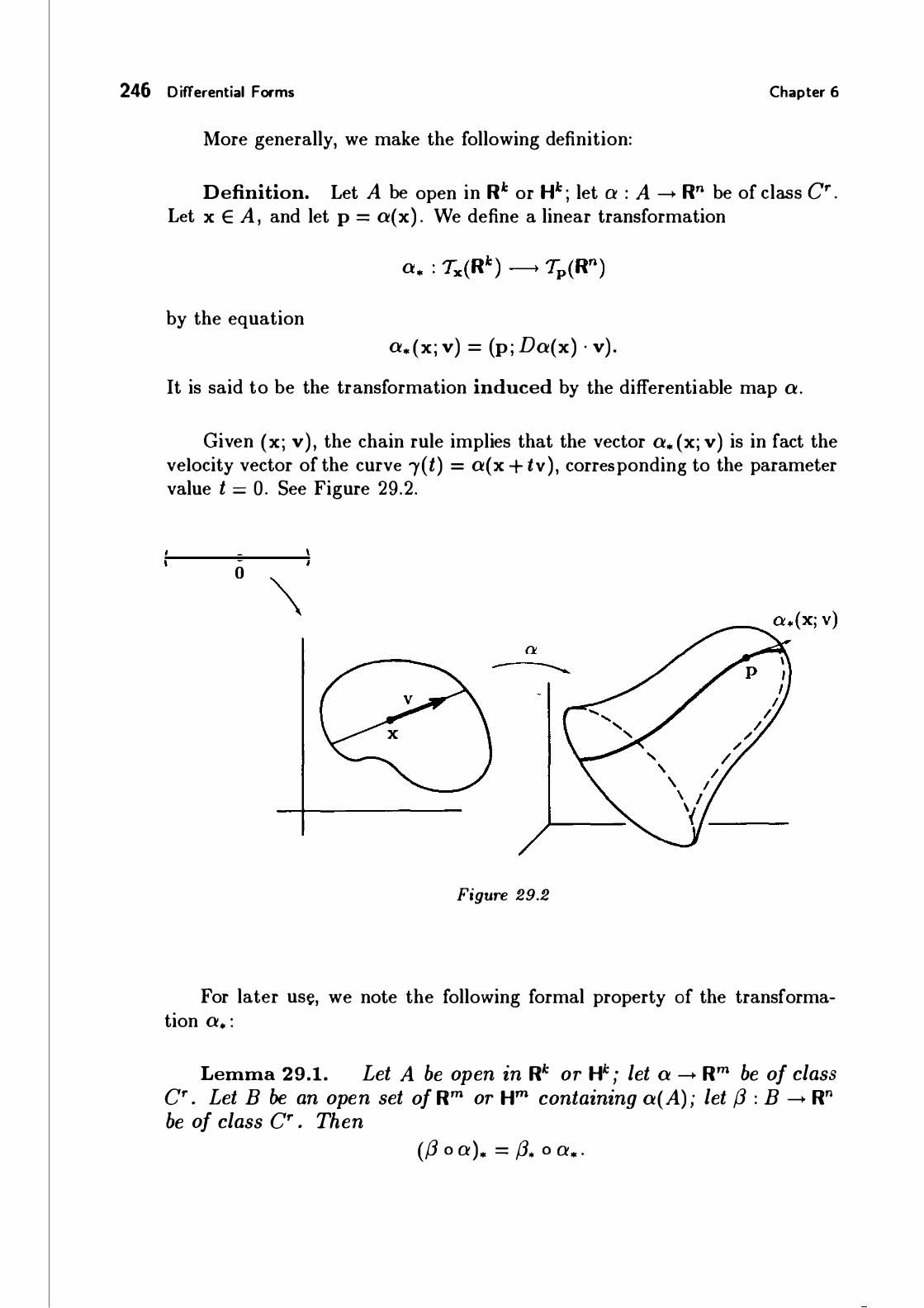
246 Differential Forms Chapter 6
More generally, we make the following definition:
Definition. Let A be open in R" or H" ; let a : A ___. Rn be of class Cr . Let x E A, and let p = a(x) . We define a linear transformation
by the equation a. (x; v) = (p ; Da(x) · v) .
It is said to be the transformation induced by the differentiable map a.
Given (x; v) , the chain rule implies that the vector a. (x; v) is in fact the velocity vector of the curve 1(t) = a(x + tv), corresponding to the parameter value t = 0. See Figure 29.2.
0
Figure 29.2
For later use, we note the following formal property of the transformation a. :
Lemma 29.1. Let A be open in R" or Hk ; let a ___. Rm be of class cr . Let B be an open set of Rm or Hm containing a( A) ; let (J : B ___. Rn be of class cr . Then
({3 o a). = (J. o a • .
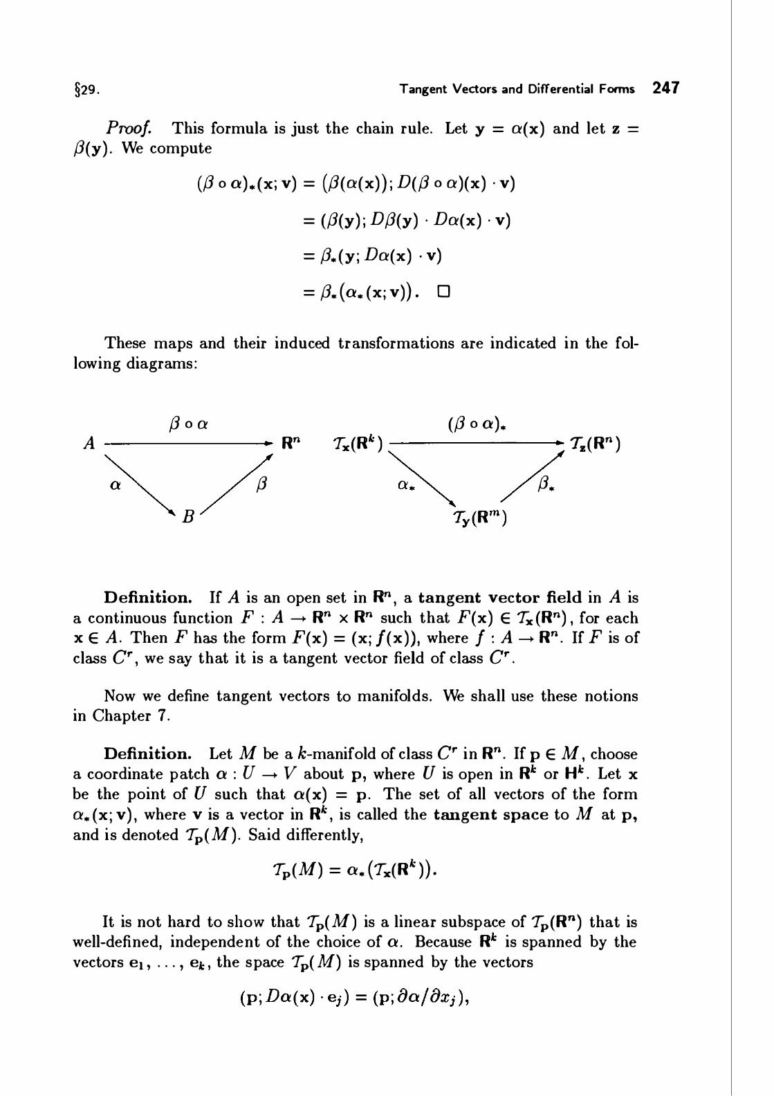
§29 . Tangent Vectors and Differential Forms 247
Proof. This formula is just the chain rule. Let y = a(x) and let z = {J(y) . We compute
((J o a). (x; v) = ({J(a(x)) ; D({J o a)(x) · v)
= ({J(y) ; D{J(y) · Da(x) · v)
= {J.(y; Da(x) · v)
= (J. (a. (x; v)) . 0
These maps and their induced transformations are indicated in the following diagrams:
{J o a ({J o a). A ________________ _. Rn Tx(Rl: ) -------- 'Tz(Rn )
(J (J.
B
Definition. If A is an open set in Rn , a tangent vector field in A is a continuous function F : A ---> Rn X Rn such that F(x) E Tx (Rn) , for each x E A. Then F has the form F(x) = (x; /(x)), where f : A __. Rn . If F is of class cr ' we say that it is a tangent vector field of class cr .
Now we define tangent vectors to manifolds. We shall use these notions in Chapter 7.
Definition. Let M be a k-manifold of class cr in Rn. If p E M, choose a coordinate patch a : U __. V about p, where U is open in R" or H" . Let x be the point of U such that a(x) = p. The set of all vectors of the form a. (x; v) , where v is a vector in R" , is called the tangent space to M at p, and is denoted Tp(M). Said differently,
Tp(M) = a. (Tx(R" )) .
It is not hard to show that Tp(M) is a linear subspace of Tp(Rn) that is well-defined, independent of the choice of a. Because R" is spanned by the vectors e1 , . . . , el: , the space Tp( M) is spanned by the vectors

248 Differential Forms
- -....
Figure 29.3
Chapter 6
for j = 1 , . . . , k . Since Da has rank k, these vectors are independent; hence they form a basis for Tv(M). Typical cases are pictured in Figure 29.3.
We denote the union of the tangent spaces Tp(M), for p E M, by T(M) ; and we call it the tangent bundle of M. A tangent vector field to M is a continuous function F : M ___. T(M) such that F(p) E Tp(M) for each p E M.
Tensor fields
Definition. Let A be an open set in Rn . A k-tensor field in A is a function w assigning, to each x E A, a k-tensor defined on the vector space Tx(Rn) . That is,
for each x. Thus w(x) is a function mapping k-tuples of tangent vectors to Rn at x into R ; as such, its value on a given k-tuple can be written in the form
W( X) ( (X j V l ) , · · . , (X j V k )) •
We require this function to be continuous as a function of (x, v1 , • • • , vk) i if it is of class cr ' we say that w is a tensor field of class cr . If it happens that w(x) is an alternating k-tensor for each x, then w is called a differential form (or simply, a form) of order k, on A.

§29. Tangent Vectors and Differential Fa-ms 249
More generally, if M is an m-manifold in Rn , then we define a k-tensor field on M to be a function w assigning to each p E M an element of C" (Tp(M)) . If in fact w(p) is alternating for each p, then w is called a differential form on M .
If w is a tensor field defined on an open set of Rn containing M , then w of course restricts to a tensor field defined on M, since every tangent vector to M is also a tangent vector to Rn . Conversely, any tensor field on M can be extended to a tensor field defined on an open set of Rn containing M; the proof, however, is decidedly non-trivial. For simplicity, we shall restrict ourselves in this book to tensor fields that are defined on open sets of Rn .
Definition. Let ei , . . . , en be the usual basis for Rn . Then ( x; ei ) , . . . , -(x; en) is called the usual basis for Tx(Rn) . We define a 1-form </>; on Rn by the equation
- -- { 0 if i -1 j' </>;(x)(x; ei ) = . . .
1 If l = J .
The forms </>I , . . . , </>n are called the elementary 1-forms on Rn. Similarly, given an ascending k-tuple I = (i. , . . . , ik) from the set { 1 , . . . , n} , we define -a k-form '1/JI on Rn by the equation
- - - -'1/JI (x) = </>;, (x) A · · · A </>;k (x) .
The forms '1/J I are called the elementary k-forms on Rn . - -Note that for each x, the 1-tensors </>I (x), . . . , </>n (x) constitute the basis
for C I ( Tx (Rn )) dual to the usual basis for Tx (Rn) , and the k-tensor �I ( x) is the corresponding
_elementary alternating tensor on Tx(Rn) .
The fact that </>; and '1/JI are of class C00 follows at once from the equations -</>; (x)(x; v) = v; , -'1/JI(x) {(x; vi ) , . . . , (x; v�: ) ) = det XI ,
where X is the matrix X = [vi · · · v�:] . If w is a k-form defined on an open set A of Rn , then the k-tensor w(x)
can be written uniquely in the form
w(x) = L bi(x)�I(x), [I)
for some scalar functions bi (x) . These functions are called the components of w relative to the standard elementary forms in Rn .

250 Differential Forms Chapter 6
Lemma 29.2. Let w be a k-form on the open set A of Rn . Then w is of class cr if and only if its component functions bl are of class cr on A .
Proof. Given w, let us express it in terms of elementary forms by the equation
-
The functions '1/JJ are of class coo . Therefore, if the functions b1 are of class cr , so is the function w. Conversely, if w is of class cr as a function of (x, v1 , . . . , v�: ) , then in particular, given an ascending k-tuple J = {j1 , . . . , i�:) from the set { 1 , . . . , n} , the function
is of class Cr as a function of x. But this function equals b1(x) . 0
Lemma 29.3. Let w and 'fJ be k-forms, and let () be an f-jorm, on the open set A of Rn . If w and 'fJ and () are of class cr , so are aw + b'fJ and w A 0.
Proof. It is immediate that aw + bTJ is of class cr , since it is a linear combination of Cr functions. To show that w A () is of class cr , one could use the formula for the wedge product given in the proof of Theorem 28 . 1 . Alternatively, one can use the preceding theorem: Let us write
and () = L CJ;j;J , [J)
where I and J are ascending k- and £-tuples, respectively, from the set { 1 , . . . , n} . Then
w A () = E E b[CJ;j;l A ;J;J . [I) [J)
To write (w A O)(x) in terms of elementary alternating tensors , we drop all terms with repeated indices, rewrite the remaining terms with indices in ascending order, and collect like terms. We see thus that each component of w A () is the sum (with signs ± 1) of functions of the form b JCJ . Thus the component functions of w A () are of class Cr . 0
Differential forms of order zero
In what follows, we shall need to deal not only with tensor fields in Rn , but with scalar fields as well. It is convenient to treat scalar fields as differential forms of order 0.

§29. Tangent Vectors and Differential Fa-ms 251
Definition. If A is open in Rn, and if f : A --+ R is a map of class cr , then f is called a s calar field in A . We also call f a differential form of order 0.
The sum of two such functions in another such, and so is the product by a scalar. We define the wedge product of two 0-forms f and g by the rule f A g = f · g, which is just the usual product of real-valued functions. More generally, we define the wedge product of the 0-form f and the k-form w by the rule
(w A /) (x) = (/ A w) (x) = /(x) · w(x) ;
this is just the usual product of the tensor w(x) and the scalar /(x) . Note that all the formal algebraic properties of the wedge product hold.
Associativity, homogeneity, and distributivity are immediate; and anticommutativity holds because scalar fields are forms of order 0:
Convention. Henceforth, we shall use Roman letters such as J, g, h to denote 0-forms, and Greek letters such as w, 'f/, () to denote k-forms for k > 0.
EXERCISES
I . Let r : R - Rn be of class Cr. Show that the velocity vector of r corresponding to the parameter value t is the vector r. (t; el ) .
2. If A is open in Rk and a : A - Rn is of class Cr , show that a.(x; v) is the velocity vector of the curve r( t) = a(x + tv) corresponding to parameter value t = 0 .
3. Let M be a k-manifold of class Cr in Rn. Let p E M. Show that the tangent space to M at p is well-defined , independent of the choice of the coordinate patch.
4. Let M be a k-manifold in Rn of class Cr . Let p E M - {)M. (a) Show that if (p; v) is a tangent vector to M, then there is a para
metrized-curve r : ( -E, E) -+ Rn whose image set lies in M, such that (p; v) equals the velocity vector of r corresponding to parameter value t = 0 . See Figure 29.4.
(b) Prove the converse. [Hint: Recall that for any coordinate patch a, the map a-1 is of class cr. See Theorem 24.1 .)
5. Let M be a k-manifold in Rn of class Cr . Let q E {)M. (a) Show that if (q; v) is a tangent vector to M at q, then there is a
parametrized-curve r : ( -E, E) - Rn' where r carries either ( -E, 0) or [0 , E) into M' such that ( q; v) equals the velocity vector of r corresponding to parameter value t = 0.

252 Differential Forms Chapter 6
Figure 29.4
(b) Prove the converse.
§30. THE D IFFERENTIAL OP ERATOR
We now introduce a certain operator d on differential forms. In general , the operator d, when applied to a k-form, gives a k+ 1 form. We begin by defining d for 0-forms.
The differential of a 0-form
A 0-form on an open set A of Rn is a function f : A -+ R. The differential df of f is to be a 1-form on A, that is, a linear transformation of Tx(Rn ) into R, for each x E A. We studied such a linear transformation in Chapter 2 . We called it the "derivative of f at x with respect to the vector v." We now look at this notion as defining a 1-form on A .
Definition. Let A be open in Rn ; let f A -+ R be a function of

§30. The Differential Operator 253
class cr . We define a 1-form df on A by the formula
df(x)(x; v) = /'(x; v) = D f(x) · v.
The 1-form df is called the differential of f. It is of class cr-I as a function of x and v.
Theorem 30.1. The operator d is linear on 0-forms.
Proof. Let f, g : A ___. R be of class cr . Let h = af + bg. Then
Dh(x) = a D f(x) + b Dg(x) ,
so that dh(x)(x; v) = a df(x)(x; v) + b dg(x)(x; v) .
Thus dh = a(df) + b(dg) , as desired. 0
Using the operator d, we can obtain a new way of expressing the elemen--tary 1-forms </>; in Rn :
- -Lemma 30.2. Let </>1 , • • • , <l>n be the elementary 1 -forms in Rn .
Let 11"; : Rn ___. R be the ith projection function, defined by the equation
11";(x . , . . . , Xn) = X;.
-Then drr; = </>; .
Proof. Since 11"; is a coo function, drr; is a 1-form of class coo . We compute
drr; (x)(x ;v) = Drr;(x) · v
-Thus drr; = </>; . 0
V1 = (0 · · · 0 1 0 · · · 0] = V; .
Now it is common in this subject to abuse notation slightly, denoting the ith projection function not by 11"; but by X; . Then in this notation, �; is equal to dx; . We shall use this notation henceforth:
Convention. If x denotes the general point of Rn , we denote the z"th projection function mapping Rn to R by the symbol X; . Then dx; equals

254 Differential Forms Chapter 6
-the elementary 1-form </>; in Rn . If I = (i1 , . . . , i�c) is an ascending k-tuple from the set { 1 , . . . , n} , then we introduce the notation
dXI - dx · A · · · A dx · - 1 1 l k
-for the elementary k-form '1/JI in Rn . The geneml k-form can then be written uniquely in the form
for some scalar functions bi .
The forms dx; and dxi are of course characterized by the equations
dx; (x) (x; v) = v; ,
dx I ( x) ( ( x; v 1 ) , . . . , ( x; v 1c )) = det X I ,
where X is the matrix X = [v1 · · · v�c] . For convenience , we extend this notation to an arbitrary k-tuple J
(j1 , . . . , i�c ) from the set { 1 , . . . , n } , sett ing
Note that whereas dxi is the differential of a 0-form, dxJ does not denote the differential of a form, but rather a wedge product of elementary 1-forms.
REMARK. Why do we call the use of X; for 7r; an abuse of notation? The reason is this: Normally, we use a single letter such as f to denote a function, and we use the symbol f(x) to denote the value of the function at the point x. That is, f stands for the rule defining the function, and f(x) denotes an element of the range of f. It is an abuse of notation to confuse the function with the value of the function.
However, this abuse is fairly common. We often speak of "the function x3 + 2x + 1" when we should instead speak of "the function f defined by the equation f(x) = x3 + 2x + 1 ," and we speak of "the function e"'" when we should speak of "the exponential function."
We are doing the same thing here. The value of the i1h projection function at the point x is the number x ; ; we abuse notation when we use X; to denote the function itself. This usage is standard , however, and we shall conform to it .
If f is a 0-form, then df is a 1-form, so it can be expressed as a linear combination of elementary 1-forms. The expression is a familiar one:
§30. The Differential Operator 25 5
Theorem 30.3. Let A be open in Rn ; let f : A ___. R be of class cr . Then
df = (D. j)dx 1 + · · · + (Dn f)dxn .
In particular, df = 0 iff is a constant function.
In Leibnitz's notation, this equation takes the form
of of df = 0 dx1 + · · · + 0 dxn o
X 1 Xn
This formula sometimes appears in calculus books, but its meaning is not explained there.
Proof. We evaluate both sides of the equation on the tangent vector (x ; v) . We have
df(x)(x; v) = D f(x) · v
by definition, whereas
n n L D;/(x) dx;(x) (x; v) = L D;/(x)v; . i = l i = l
The theorem follows. 0
The fact that df is only of class cr-I if f is of class cr is very inconvenient. It means that we must keep track of how many degrees of differentiability are needed in any given argument. In order to avoid these difficulties, we make the following convention:
Convention. Henceforth, we restrict ourselves to manifolds, maps, vector fields, and forms that are of class coo .
The differential of a k-form
We now define the differential operator d in general. It is in some sense a generalized directional derivative. A formula that makes this fact explicit appears in the exercises. Rather than using this formula to define d, we shall instead characterize d by its formal properties , as given in the theorem that follows.
Definition. If A is an open set in Rn , let nk (A) denote the set of all k-forms on A (of class C00). The sum of two such k-forms is another k-form, and so is the product of a k-form by a scalar. It is easy to see that O" (A) satisfies the axioms for a vector space; we call it the linear space of k-forms on A.

256 Differential Forms Chapter 6
Theorem 30.4. Let A be an open set in Rn . There exists a unique linear transformation
defined for k > 0, such that: (1) Iff is a 0-form, then df is the 1-form
df(x)(x; v) = Df(x) · v.
(2) If w and 'f/ are forms of orders k and i, respectively, then
(3) For every form w, d(dw) = 0.
We call d the differential operator, and we call dw the differential of w.
Proof. Step 1 . We verify uniqueness . First, we show that conditions (2) and (3) imply that for any forms w. , . . . , W1c , we have
If k = 1 , this equation is a consequence of (3) . Supposing it true for k - 1, we set 'f/ = (dw2 1\ · · · I\ dwk) and use (2) to compute
The first term vanishes by (3) and the second vanishes by the induction hypothesis.
Now we show that for any k-form w, the form dw is entirely determined by the value of d on 0-forms, which is specified by ( 1 ) . Since d is linear, it suffices to consider the case w = f dx I · We compute
dw = d(/ dx1) = d(/ 1\ dxi)
= df 1\ dx1 + f 1\ d(dx1)
= df 1\ dx1 ,
by (2) ,
by the result just proved. Thus dw is determined by the value of d on the 0-form f.

§30. The Differential Operator 25 7
Step 2. We now define d. Its value for 0-forms is specified by ( 1 ) . The computation just made tells us how to define it for forms of positive order: If A is an open set in Rn and if w is a k-form on A, we write w uniquely in the form
and define dw = L d/J A dx I ·
[I) We check that dw is of class coo . For this purpose, we first compute
n dw = L [L (Di /)dxi ] A dxi.
[I) j=l
To express dw as a linear combination of elementary k + 1 forms, one proceeds as follows: First, delete all terms for which j is the same as one of the indices in the k-tuple I. Second , take the remaining terms and rearrange the dx; so the indices are in ascending order. Third, collect like terms. One sees in this way that each component of dw is a linear combination of the functions D if, so that it is of class C00 • Thus dw is of class C00 • (Note that if w were only of class cr ' then dw would be of class cr- l . )
We show d is linear on k-forms with k > 0. Let
be k-forms. Then
d(aw + b'f/) = d L (a /I + bgi)dxi [I)
= L d(a/J + bgi) A dxi by definition, (I]
= L (a d/J + b dgi) A dx I since d is linear on 0-forms, [I)
= a dw + b d'f/.
Step 3. We now show that if J is an arbitrary k-tuple of integers from the set { 1 , . . . , n} , then

258 Differential Forms Chapter 6
Certainly this formula holds if two of the indices in J are the same, since dxJ = 0 in this case. So suppose the indices in J are distinct. Let I be the k-tuple obtained by rearranging the indices in J in ascending order; let 1r be the permutation involved. Anticommutativity of the wedge product implies that dxi = (sgn 1r)dx1 . Because d is linear and the wedge product is homogeneous, the formula d(/ A dx I) = df A dx I, which holds by definition, implies that
(sgn 1r) d(f A dxJ) = (sgn 1r) df A dxJ .
Our desired result follows.
Step 4. We verify property (2) , in the case k compute
n
d(/ A g) = L Di(/ · g)dxi j : l
n n
j : l j= l
= (df) A g + f A (dg) .
0 and f 0. We
Step 5. We verify property (2) in generaL First, we consider the case where both forms have positive order. Since both sides of our desired equation are linear in w and in 'f/, it suffices to consider the case
We compute
d(w A 'T/) = d(f g dxi A dxJ)
= d(fg) A dxi A dxJ by Step 3,
= (df A g + f A dg) A dxi A dxJ by Step 4,
= (df A dxi) A (g A dxJ) + (-1)" (/ A dxi) A (dg A dxJ)
= dw A 'f/ + ( - 1)"w A d'f/.
The sign ( - 1 )" comes from the fact that dx I is a k-form and dg is a 1-form. Finally, the proof in the case where one of k or f is zero proceeds as in the
argument just given. If k = 0, the term dxi is missing from the equations, while if e = 0, the term dx1 is missing. We leave the details to you.

§30 . The Differential Operator 259
Step 6. We show that if f is a 0-form, then d( df) = 0. We have
n d(df) = d L: Dif dxi ,
j=l n
= I: d(Dif) A dxi by definition, i= l n n
= I: I: D;Dif dx; A dxi . i= l i=l
To write this expression in standard form, we delete all terms for which i = j, and collect the remaining terms as follows:
d(df) = I: (D;Di f - DiDd)dx; A dxi . i<j
The equality of the mixed partial derivatives implies that d(df) = 0. Step 7. We show that if w is a k-form with k > 0, then d(dw) = 0.
Since d is linear, it suffices to consider the case w = f dx I · Then
d(dw) = d(df A dxi)
= d( df) A dx I - df A d( dx I) , by property (2) . Now d(df) = 0 by Step 6, and
d( dx I) = d( 1) A dx I = 0
by definition. Hence d( dw) = 0. 0
Definition. Let A be an open set in Rn . A 0-form f on A is said to be exact on A if it is constant on A; a k-form w on A with k > 0 is said to be exact on A if there is a k - 1 form () on A such that w = d(). A k-form w on A with k > 0 is said to be closed if dw = 0.
Every exact form is closed; for if f is constant, then df = 0, while if w = d(), then dw = d( d()) = 0. Conversely, every closed form on A is exact on A if A equals all of Rn, or more generally, if A is a "star-convex" subset of Rn . (See Chapter 8.) But the converse does not holds in general, as we shall see. If every closed k-form on A is exact on A, then we say that A is homologically trivial in dimension k. We shall explore this notion further in Chapter 8.

260 Differential Forms Chapter 6
EXAMPLE 1 . Let A be the open set in R2 consisting of all points (x, y) for which x ::/= 0. Set f(x, y) = xl lxl for (x, y) E A. Then f is of class Coo on A, and df = 0 on A. But f is not exact on A because f is not constant on A.
EXAMPLE 2. Exactness is a notion you have seen before. In differential equations, for example, the equation
P(x, y) dx + Q(x, y) dy = 0
is said to be exact if there is a function f such that P = {) f I {)x and Q = {) f I {)y. In our terminology, this means simply that the 1-form P dx + Q dy is the differential of the 0-form J, so that it is exact.
Exactness is also related to the notion of conservative vector fields. In R3, for example, the vector field
- - - -F = Pi + Qj + Rk
is said to be conservative if it is the gradient of a scalar field J, that is, if
P = 8fl8x and Q = 8fl8y and R = 8fl8z .
This is precisely the same as saying that the form P dx + Q dy + Rdz is the differential of the 0-form f.
We shall explore further the connection between forms and vector fields in the next section.
EX ERCISES
1 . Let A be open in Rn.
(a) Show that Ok(A) is a vector space.
(b) Show that the set of all Coo vector fields on A is a vector space.
2 . Consider the forms
w = xy dx + 3 dy - yz dz,
7J = x dx - yz2 dy + 2x dz,
in R3 . Verify by direct computation that
d(dw) = 0 and d(w A 7J) = (dw) A 7J - w A d7J.
3. Let w be a k-form defined in an open set A of Rn . We say that w vanishes at x if w(x) is the 0-tensor.
(a) Show that if w vanishes at each x in a neighborhood of Xo, then dw vanishes at Xo .

§30. The Differential Operator 261
(b) Give an example to show that if w vanishes at Xo , then dw need not vanish at Xo .
4. Let A = R2 - 0; consider the 1-form in A defined the equation
(a) Show w is closed .
(b) Show that w is exact on A.
*5. Prove the following:
Theorem. Let A = R2 - 0; let
in A . Then w is closed, but not exact, in A . Proof. (a) Show w is closed .
(b) Let B consist of R2 with the non-negative x-axis deleted. Show that for each (x, y) E B, there is a unique t with 0 < t < 27r such that
denote this value of t by <J;(x, y). (c) Show that </> is of class Coo . [Hint: The inverse sine and inverse
cosine functions are of class Coo on the intervals ( -1r /2, 1r /2) and (0, 1r), respectively.)
(d) Show that w = d<J; in B . [Hint: We have tan </> = yfx if x ::/= 0 and cot </> = xfy if y ::/= 0.]
(e) Show that if g is a closed 0-form in B, then g is constant in B. [Hint: Use the mean-value theorem to show that if a is the point ( -1 , 0) of R2, then g(x) = g(a) for all x E B.]
(f) Show that w is not exact in A. [Hint: If w = df in A, then f - </> is constant in B. Evaluate the limit of /(1 , y) as y approaches 0 through positive and negative values.)
6. Let A = Rn - 0. Let m be a fixed positive integer. Consider the following n - 1 form in A:
n 7J = L ( - 1 )'-1 f; dx1 A · · · A ;[;, A · · · A dxn,
i=l
-where f; (x) = x;f l lxllm, and where dx; means that the factor dx; is to be omitted.
(a) Calculate d7J. (b) For what values of m is it true that d7J = 0? (We show later that 7J
is not exact.)

262 Differential Forms Chapter 6
*7. Prove the following, which expresses d as a generalized "directional derivative" :
Theorem. Let A be open in Rn; let w be a k- 1 form in A. Given Vi , . . . , Vk E Rn, define
h(x) = dw(x) ((x; vd, . . . , (x; vk )) ,
-Yi(x) = w(x) ((x; vd , . . . , (x; vi ), . . . , (x; vk )) ,
wh ere a means that the component a is to be omitted. Then
k h(x) = L ( -1)1-1 Dgi (x) · vi .
;= 1
Proof. (a) Let X = [v1 · · · Vk] · For each j, let Y, = [vi · · · Vj · · · Vk]· Given ( i, i1 , . . . , ik-1 ) , show that
k det X(i, i. , . . . , ik-d = L (-I )l-1 v;i det Y, (i. , . . . , ik-d ·
i=l
(b) Verify the theorem in the case w = f dx1 . (c) Complete the proof.
*§31 . A P PL ICAT ION TO VECTOR AND SCALAR FIELDS
Finally, it is time to show that what we have been doing with tensor fields and forms and the differential operator is a true generalization to Rn of familiar facts about vector analysis in R3 . We will use these results in §38, when we prove the classical versions of Stokes' theorem and the divergence theorem.
We know that if A is an open set in Rn, then the set n" (A) of k-forms on A is a linear space. It is also easy to check that the set of all C00 vector fields on A is a linear space. We define here a sequence of linear transformations from scalar fields and vector fields to forms. These transformations act as operators that "translate" theorems written in the language of scalar and vector fields to theorems written in the language of forms, and conversely.
We begin by defining the gradient and the divergence operators in Rn.

§31 . Application to Vector and Scalar Fields 263
Definition. Let A be open in Rn . Let f : A --> R be a scalar field in A. We define a corresponding vector field in A, called the gradient of f, by the equation
(grad /)(x) = (x; D./(x)ei + · · · + Dnf(x)en ) ·
If G(x) = (x; g(x)) is a vector field in A, where g : A --> Rn is given by the equation
then we define a corresponding scalar field in A, called the divergence of G, by the equation
These operators are of course familiar from calculus in the case n = 3 . The following theorem shows how these operators correspond to the operator d:
Theorem 31.1 . Let A be an open set in Rn . There exist vector space isomorphisms a; and (Ji as in the following diagram:
such that
Scalar fields in A
lgrad
Vector fields in A
Vector fields in A
Scalar fields in A
ao -----+
a, -----+
13 ... -----+
f2°(A)
ld
f21 (A)
d o no = a1 o grad and d o fJn- I = fJn o div.
Proof. Let f and h be scalar fields in A; let
F(x) = (x; L f; (x)e;) and G(x) = (x; L g;(x)e;)

264 Differential Forms Chapter 6
be vector fields in A. We define the transformations a; and {Jj by the equa-tions
aof = /,
n a 1 F = L f;dx; ,
i= l
n f3n- 1G = L ( -l)i- 1g; dx1 A · · · A dx; A · · · A dxn ,
i=l
(As usual, the notation a means that the factor a is to be omitted. ) The fact that each a; and (Ji is a linear isomorphism, and that the two equations hold , is left as an exercise. 0
This theorem is all that can be said about applications to vector fields in general . However, in the case of R3, we have a "curl" operator, and something more can be said .
Definition. Let A be open in R3; let
F(x) = (x; L /; (x)e;)
be a vector field in A . We define another vector field in A, called the curl of F, by the equation
A convenient trick for remembering the definition of the curl operator is to think of it as obtained by evaluation of the symbolic determinant
For R3, we have the following strengthened version of the preceding theorem:
Theorem 31.2. Let A be an open set in R3 • There exist vector space isomorphisms a; and f3i as in the following diagram:

§31 .
Scalar fields in A
lgrad
Vector fields in A
lcurl
Vector fields in A
1 div
Scalar fields in A
Application to Vector and Scalar Fields 265
ao f2° (A) -
ld
a, f21 (A) -
ld
fJl f22 (A) -
ld
fJ3 f23(A) -
such that
d o ao = a1 o grad and d o a1 = (32 o curl and d o fJ2 = (33 o div.
Proof. The maps a; and (Ji are those defined in the proof of the preceding theorem. Only the second equation needs checking; we leave it to you. 0
EXER CISES
1 . Prove Theorems 31 .1 and 31 .2 . 2. Note that in the case n = 2, Theorem 31 .1 gives us two maps a1 and fJ1
from vector fields to 1-forms. Compare them.
3. Let A be an open set in R3 . (a) Translate the equation d(dw) = 0 into two theorems about vector
and scalar fields in R3 . (b) Translate the condition that A is homologically trivial in dimension k
into a statement about vector and scalar fields in A. Consider the cases k = 0 , 1 , 2.
4. For R4, there is a way of translating theorems about forms into more familiar language, if one allows oneself to use matrix fields as well as vector fields and scalar fields. We outline it here. The complications involved may help you understand why the language of forms was invented to deal with Rn in general.
A square matrix B is said to be skew-symmetric if B1r = -B. Let A be an open set in R4 • Let S(A) be the set of all Coo functions H mapping A into the set of 4 by 4 skew-symmetric matrices. If h;j (x) denotes the entry of H(x) in row i and column j, define r2 : S(A) -02(A) by the equation
r2(H) = L h;; (x) dx; 1\ dx) . i<j

266 Differential Forms Chapter 6
(a) Show r2 is a linear isomorphism.
(b) Let O:o , o:1 , /33 , /34 be defined as in Theorem 31 . 1 . Define operators "twist" and "spin" as in the following diagram:
such that
Vector fields in A
llwi•l S(A)
l•pin Vector fields in A
O J -----
d o o:1 = r2 o twist and d o r2 = /33 o spm.
(These operators are facetious analogues in R4 of the operator "curl" in R3 .)
5 . The operators grad, curl, and div, and the translation operators 0:; and /3i , seem to depend on the choice of a basis in Rn, since the formulas defining them involve the components of the vectors involved relative to the basis e1 , · · · , en in Rn. However, they in fact depend only on the inner product in Rn and the notion of right-handedness, as the following exercise shows.
Recall that the k-volume function V(x1 , . . . , Xk ) depends only on the inner product in Rn. (See the exercises of §21 . )
(a) Let F(x) = (x; f(x)) be a vector field defined in an open set of Rn. Show that 0:1 F is the unique 1-form such that
o:1 F(x)(x; v) = (f(x) , v} . (b) Let G(x) = (x; g (x)) be a vector field defined in an open set of Rn.
Show that /3n-1 G is the unique n - 1 form such that
/3n-1G(x) ((x; vd , . . . , (x; vn-d) = E · V(g(x) , vl , . . . , Vn-1 } , where f = +1 if the frame (g(x), V1 , . . . , Vn-1 } is right-handed, and f = -1 otherwise.
(c) Let h be a scalar field defined in an open set of Rn. Show that f3nh is the unique n-form such that
/3nh(x) ((x; v1 ) , • • • , (x; vn)) = E · h(x) · V(vl , . . . , Vn), where f = +I if (v1 , . . . , Vn) is right-handed, and f = -1 otherwise.
(d) Conclude that the operators grad and div (and curl if n = 3) depend only on the inner product in Rn and the notion of right-handedness in Rn. [Hint: The operator d depends only on the vector space structure of Rn.)

§32. The Action of a Differentiable Map 26 7
§32 . T H E ACTION OF A D I FFERENTIABLE MAP
If a : A - Rn is a C00 map, where A is open in R", then a gives rise to a linear transformation a. mapping the tangent space to R" at x into the tangent space to Rn at a(x). Furthermore, we know that any linear transformation T : V - W of vector spaces gives rise to a dual transformation T* : Al (W) - Al(V) of alternating tensors. We combine these two facts to show how a C00 map a gives rise to a dual transformation of forms, which we denote by a* . The transformation a* preserves all the structure we have imposed on the space of forms-the vector space structure, the wedge product, and the differential operator.
Definition. Let A be open in R" ; let a : A - Rn be of class C00; let B be an open set of Rn containing a( A). We define a dual transformation of forms
as follows: Given a 0-form f : B - R on B, we define a 0-form a* f on A by setting (a* /)(x) = f(a(x)) for each x E A. Then, given an f-form w on B with f > 0, we define an £-form a*w on A by the equation
(a*w) (x) ((x ;v1 ) , . . . , (x ; vl )) = w (a(x)) (a. (x; v1 ) , . . . , a. (x; vt ) ) .
Since f and w and a and Da are all of class coo , so are the forms a* f and a*w. Note that if f and w and a were of class Cr , then a* f would be of class cr but a*w would only be of class cr - I . Here again it is convenient to have restricted ourselves to C00 maps.
Note that if a is a constant map, then a* f is also constant, and a*w is the 0-tensor.
The relation between a* and the dual of the linear transformation a. is the following: Given a : A - Rn of class coo , with a(x) = y, it induces the linear transformation
this transformation in turn gives rise to a dual transformation of alternating tensors,
If w is an £-form on B, then w(y) is an alternating tensor on Ty(Rn) , so that T* (w(y)) is an alternating tensor on Tx(R"). It satisfies the equation
T* (w(y)) = (a*w)(x) ;

268 Chapter 6
for
T* (w(y)) ((x ; v. ), . . . , (x ; vl )) = w(a(x)) (a. (x; v1 ), . . . , a.(x ; vl ))
= (a*w)(x) ((x ;v1 ) , . . . , (x; vl )) .
This fact enables us to rewrite earlier results concerning the dual transformation T* as results about forms:
Theorem 32.1 . Let A be open in R" ; let a : A --+ Rm be a C00 map. Let B be open in Rm and contain a(A); let (J : B --+ Rn be a C00 map. Let w, 'f/, () be forms defined in an open set C of Rn containing {J(B); assume w and 'f/ have the same order. The transformations a* and {J* have the following properties:
( 1 ) {J* (aw + b'T/) = a({J*w) + b(fJ*'T/) · (2) {J* (w A ()) = {J*w A {J*(). (3) ({J o a)*w = a* ({J*w) .
Proof. See Figure 32 . 1 . In the case of forms of positive order, properties (1) and (3) are merely restatements, in the language of forms, of Theorem 26.5, and (2) is a restatement of (6) of Theorem 28.1 .
Checking the properties when some or all of the forms have order zero is a computation we leave to you. D
- - - - - -...
Figure 32. 1

§32. The Action of a Differentiable Map 269
This theorem shows that a* preserves the vector space structure and the wedge product. We now show it preserves the operator d. For this purpose (and later purposes as well) , we obtain a formula for computing a*w. If A is open in R" and a : A --+ Rn , we derive this formula in two cases-when w is a 1-form and when w is a k-form. This is all we shall need . The general case is treated in the exercises.
Since a* is linear and preserves wedge products, and since a* f equals f o a, it remains only to compute a* for elementary 1-forms and elementary k-forms. Here is the required formula:
Theorem 32.2. Let A be open in R"; let a : A --+ Rn be a coo map. Let x denote the general point of R"; let y denote the general point of Rn . Then dx; and dy; denote the elementary 1-forms in R" and Rn , respectively.
(a) a* (dy;) = da; . (b) If I = (i1 , . • • , i�.:) is an ascending k-tuple from the set { 1 , . . . , n} ,
then
where {}a[ - a(a;, , . . . , a;k ) ax - a(x . , . . . ' x�:)
.
Proof. (a) Set y = a(x). We compute the value of a* (dy;) on a typical tangent vector as follows:
(a* (dyi )} (x)(x ; v) = dy; (y) (a. (x; v))
It follows that
= ith component of (Da(x) · v) l:
= L Dia;(x) · Vj i= l
l: '"' aa; = LJ ax ·
(x) dxj (x)(x; v) . j= l 1
• d ) 2:::.::" aa; d a ( y; = {} xi .
X · i=l 1
By Theorem 30.3, the latter expression equals da; .

270 Chapter 6
(b) The form a* ( dy!) is a k-form defined in an open set of R", so it has the form
a* ( dy!) = h dx1 A · · · A dx�: for some scalar function h . If we evaluate the right side of this equation on the k-tuple (x; e1 ) , . . . , (x ; el: ) , we obtain the function h(x) . The theorem then follows from the following computation :
h(x) = (a* (dy!)) (x) ((x ; e. ) , . . . , (x; e�: )) = dyi(y) (a. (x; e1 ) , • • • , a. (x; el: ))
= dyi(Y) ((y; aafax.) , . . . , (y; aafaxk)) = det[Da(x)]I
a a[ = det ax . 0
It is easy to remember the formula (a); to compute a*(dy;) , one simply takes the form dy; and makes the substitution y; = a;(x)!
Note that one could compute a*( dy! ) by the formula
= da;, A · · · A da;k ,
but the computation of this wedge product is laborious if k > 2 .
Theorem 32.3. Let A be open in R"; let a : A --+ Rn be of class coo . If w is an f-form defined in an open set of Rn containing a(A), then
a* (dw) = d(a*w).
Proof. Let x denote the general point of R"; let y denote the general point of Rn .
Step 1 . We verify the theorem first for a 0-form f. We compute the left side of the equation as follows:
n a*(df) = a* (L (D;f) dy;)
i=l
n = L ((D;f ) o a) da; .
i= l

§32. The Action of a Differentiable Map 271
Then we compute the right side of the equation. We have
d( a* f) = d(! o a) l:
= L Di (/ o a) dxi . j= l
We now apply the chain rule. Setting y = a(x), we have
D(! o a)(x) = D /(y) · Da(x); since D(! o a) and D f are row matrices, it follows that
Thus
Di (/ o a)(x) = D f(y) · (jth column of Da(x))
n = L D;f(y) · Dja;(x).
i= l n
DiU o a) = L ((D;J) o a) · Dia;. i=l
Substituting this result in the equation (**) , we have
(* * *) l: n
d(a* f) = L L ((D;f) o a) . Diai dxi i= 1 i=l
n = L ((D;f) o a) da;.
i=l Comparing (*) and (* * *) , we see that a*(df) = d(a* f).
Step 2. We prove the theorem for forms of positive order. Since a* and d are linear, it suffices to treat the case w = f dYJ , where I = (i1 , . • • , it ) is an ascending £-tuple from the set { 1 , . . . , n } . We first compute
a*(dw) = a*(df A dy! )
= a*(df) A a*(dyi ) .
On the other hand,
(tt) d(a*w) = d[a* (/ A dy! )] = d[( a* f) A a* ( dyi )]
= d(a* f) A a* (dyl ) + (a* f) A 0,

272 Chapter 6
smce d(a* (dyl )) = d(da;, A · · · A da;l ) = 0.
The theorem follows by comparing (t) and (tt) and using the result of Step 1 . D
We now have the algebra of differential forms at our disposal , along with differential operator d. The basic properties of this algebra and the operator d, as summarized in this section and §30, are all we shall need in the sequel .
It is at this point, where one is dealing with the action of a differentiable map, that one begins to see that forms are in some sense more natural objects to deal with than are vector fields. A C00 map o: : A --+ Rn , where A is open in R" , gives rise to a linear transformation o:. on tangent vectors. But there is no way to obtain from a a transformation that carries a vector field on A to a vector field on o:(A). Suppose for instance that F(x) = (x; f(x)} is a vector field in A. If y is a point of the set B = o:(A) such that y = o:(x. ) = o:(x2 ) for two distinct points x1 , x2 of A, then a. gives rise to two (possibly different) tangent vectors a. (x1 ; f(x. )) and o:. (x2 ; /(x2 )) at y! See Figure 32.2.
0:
Figure 32.2
This problem does not occur if a : A --+ B is a diffeomorphism. In this case, one can obtain an induced map a. on vector fields. One assigns to the vector field F on A, the vector field G = a.F on B defined by the equation
A scalar field h on A gives rise to a scalar field k = a.h on B defined by the equation k = hoo:-1 • The map a. is not however very natural, for it does not in general commute with the operators grad , curl, and div of vector calculus, nor with the "translation" operators a; and (Ji of §3 1 . See the exercises.

§32. The Action of a Differentiable Map 273
EXERCIS ES
1 . Prove Theorem 32.1 when w and 7J have order zero and when 9 has order zero.
2. Let 0: : R3 - R6 be a Coo map. Show directly that
do:1 A do:3 A do:s = ( det Do:( I , 3 , 5)) dx1 A dx2 A dx3 .
3. In R3, let w = xy dx + 2z dy - y dz .
Let 0: : R2 - R3 be given by the equation
o:(u, v) = (uv, u2 , 3u + v).
Calculate dw and o:*w and o:*(dw) and d(o:*w) directly.
4. Show that (a) of Theorem 32.2 is equivalent to the formula o:* (dy;) = d(o:*y;), where y; : Rn - R is the i1h projection function in Rn.
5. Prove the following formula for computing o:*w in general:
Theorem. Let A be open in Rk; let o: : A - Rn be of class coo. L et x denote the general point of Rk; let y denote the general point of Rn. If I = (i1 , . . . , it) is an ascending l- tuple from the set { 1 , . . . , n} , then
Here J = (j1 , . . . , jt) is an ascending l-tuple from the set {I , . . . , k} and
{)o:l {)( 0:;, ' . . . ' O:;l ) {)xJ = {}(xi, . . . , Xjl ) '
*6. This exercise shows that the transformations O:; and /3i of §31 do not in general behave well with respect to the maps induced by a diffeomorphism 0:.
Let o: : A - B be a diffeomorphism of open sets in Rn. Let x denote the general point of A, and let y denote the general point of B. If F(x) = (x; f(x)) is a vector field in A, let G(y) = o:. ( F( o:-1 (y))) be the corresponding vector field in B.
(a) Show that the 1-forms 0:1 G and 0:1 F do not in general correspond under the map o:•. Specifically, show that o:* (o:1 G) = o:1 F for all F if and only if Do:(x) is an orthogonal matrix for each x. [Hint: Show the equation o:• ( 0:1 G) = 0:1 F is equivalent to the equation
Do:(x)1 r • Do:(x) · f(x) = f(x) .]
(b) Show that o:• (f3n-1 G) = f3n-1 F for all F if and only if det Do: = + 1 . [Hint: Show the equation o:• (/3n-1 G) = f3n-1 F is equivalent to the equation f(x) = (det Do:(x)) · f(x) .]

27 4 Chapter 6
(c) If h is a scalar field in A, let k = h o a-1 be the corresponding scalar field in B. Show that a.(f3nk) = f3nh for all h if and only if det Da = +I.
7. Use Exercise 6 to show that if a is an orientation-preserving isometry of Rn , then the operator a* on vector fields and scalar fields commutes with the operators grad and div, and with curl if n = 3. (Compare Exercise 5 of §31.)

Stokes' Theorem
We saw in the last chapter how k-forms provide a generalization to Rn of the notions of scalar and vector fields in R3, and how the differential operator d provides a generalization of the operators grad, curl, and div. Now we define the integral of a k-form over a k-manifold; this concept provides a generalization to Rn of the notions of line and surface integrals in R3 . Just as line and surface integrals are involved in the statements of the classical Stokes' theorem and divergence theorem in R3 , so are integrals of k-forms over k-manifolds involved in the generalized version of these theorems.
We recall here our convention that all manifolds, forms, vector fields, and scalar fields are assumed to be of class C00 •
§33. I NTEGRATING FORMS OVER PARAM ETRIZED-MANIFOLDS
In Chapter 5 , we defined the integral of a scalar function f over a manifold , with respect to volume. We follow a similar procedure here in defining the integral of a form of order k over a manifold of dimension k . We begin with parametrized-manifolds.
First let us consider a special case.
Definition. Let A be an open set in R" ; let 'f/ be a k-form defined in A. Then 'f/ can be written uniquely in the form
275

276 Stokes' Theorem Chapter 7
We define the integral of 'f/ over A by the equation
provided the latter integral exists.
This definition seems to be coordinate-dependent; in order to define fA 'f/, we expressed 'f/ in terms of the standard elementary 1-forms dx; , which depend on the choice of the standard basis e1 , . . . , e�: in R" . One can, however, formulate the definition in a coordinate-free fashion. Specifically, if a1 , . . . , al: is any right-handed orthonormal basis for R" , then it is an elementary exercise to show that
I 'f/ = I 'f/(x) ((x ; a1 ) , • • • , (x; a�:)) . jA lxEA Thus the integral of 'f/ does not depend on the choice of basis in R" , although it does depend on the orientation of R" .
We now define the integral of a k-form over a parametrized-manifold of dimension k .
Definition. Let A be open in R" ; let a : A --+ Rn be of class C00 • The set Y = a(A), together with the map a, constitute the parametrizedmanifold Ya . If w is a k-form defined in an open set of Rn containing Y, we define the integral of w over Ya by the equation
I w = I a*w, }y" jA provided the latter integral exists. Since a* and fA are linear, so is this integral .
We now show that the integral is invariant under reparametrization , up to sign.
Theorem 33.1. Let g : A --+ B be a diffeomorphism of open sets in R" . Assume det Dg does not change sign on A. Let (J : B --+ Rn be a map of class coo; let Y = {J(B). Let a = (J o g; then a : A --+ Rn and Y = a( A) . If w is a k-form defined in an open set of Rn containing Y, then w is integrable over Y.a if and only if it is integrable over Ya; in this case,
I w = ± I w, }y" }yfj

§33. Integrating Forms over Parametrized-Manifolds 277
0:
A • X
B
Figure 33.1
where the sign agrees with the sign of det Dg .
........ ', ' ' ' ' '
\ \ I
Proof Let x denote the general point of A; let y denote the general point of B. See Figure 33 . 1 . We wish to show that
i o:*w = t: L
(J*w,
where t: = ±1 and agrees with the sign of det Dg. If we set 'f/ = {J*w, then this equation is equivalent to the equation
L g·, = "l ,. Let us write 'f/ in the form 'f/ = f dy1 A · · · A dyl: . Then
g* 'f/ = (/ o g)g* (dy1 A . . · A dyk ) = (! o g) det(Dg) dx1 A · · · A dx�: .
(Here we apply Theorem 32.2, in the case k = n.) Our equation then takes the form
L (! o g) det Dg = t: l f.
This equation follows at once from the change of variables theorem, since det Dg = t: ldet Dg l . D
We remark that if A is connected (that is, if A cannot be written as the union of two disjoint nonempty open sets), then the hypothesis that det Dg does not change sign on A is automatically satisfied . For the set of points where det Dg is positive is open, and so is the set of points where it is negative.
This integral is fairly easy to compute in practice. One has the following result:

278 Stokes' Theorem Chapter 7
Theorem 33.2. Let A be open in R"; let a : A --+ Rn be of class coo; let Y = a( A) . Let x denote the general point of A; and let z denote the general point of Rn. If
w = f dz1 is a k-form defined in an open set of Rn containing Y, then
[ w = [ (/ o a) det(aaJ/ax) . }y" }A Proof. Applying Theorem 32.2, we have
a*w = (/ o a) det(aaJ/ ax) dx 1 A . . · A dx�: . The theorem follows. D
The notion of a k-form is a rather abstract one; the notion of its integral over a parametrized-manifold is even more abstract. In a later section (§36) we discuss a geometric interpretation of k-forms and of their integrals that gives some insight into their intuitive meaning.
REMARK. We can now make sense of the "dx" notation commonly used in single-variable calculus. If 7J = f dx is a 1-form defined in the open interval A = (a , b) of the real line R, then
by definition. That is,
where the notation on the left denotes the integral of a form; and the notation on the right denotes the integral of a function! They are equal by definition. Thus the "dx" notation used in connection with single integrals in calculus makes perfect sense once one has studied differential forms.
One can also make sense of the notation commonly used in calculus to denote a line integral. Given a 1-form P dx + Q dy + R dz, defined in an open set A of R3 , and given a parametrized-curve r : (a , b) - A, one has by the preceding theorem the formula
f P dx + Q dy + R dz Jc.., = J [P(r(t )) dltl + Q(r(t)) dlt2 + R(r(t )) dlt3 J dt ,
( a,b)

§33. Integrating Forms over Parametrized-Manifolds 279
where C is the image set of r. This is just the formula given in calculus for evaluating the line integral fc P dx + Q dy + R dz. Thus the notation used for line integrals in calculus makes perfect sense once one has studied differential forms.
It is considerably more difficult , however, to make sense of the "dx dy" notation commonly used in calculus when dealing with double integrals. If f is a continuous bounded function defined on a subset A of R2, it is common in calculus to denote the integral of f over A by the symbol
j 1 f(x, y) dx dy.
Here the symbol "dx dy" has no independent meaning, since the only product operation we have defined for 1-forms is the wedge product. One justification for this notation is that it resembles the notation for the iterated integral. And indeed, if A is the interior of a rectangle (a, b] x [c, d], then we have the equation 1dr1b f(x, y) dx] dy = 1 J.
by the Fubini theorem. Another justification for this notation is that it resembles the notation for the integral of a 2-form, and one has the equation
1 f dx A dy = 1 f
by definition. But a difficulty arises when one reverses the roles of x and y. For the iterated integral, one has the equation
and for the integral of a 2-form, one has the equation
l f dy A dx = - l f !
Which rule should one follow in dealing with the symbol
j 1 f(x, y) dy dx ?
Which ever choice one makes, confusion is likely to occur. For this reason, the "dx dy" notation is one we shall not use.
One could, however, use the "dV" notation introduced in Chapter 5 without ambiguity. If A is open in Rk, then A can be considered to be a parametrized-manifold that is parametrized by the identity map o: : A - A! Then
{ j dV = 1 (! o o:)V(D(o:)) = 1 j, }A� A A since D(o:) is the identity matrix. Of course, the symbol d used here bears no relation to the differential operator d.

280 Stokes' Theorem Chapter 7
EXERCISES
1. Let A = (0, 1 )2 • Let 0: : A - R3 be given by the equation
o:(u, v) = (u , v, u2 + v2 + I) .
Let Y be the image set of 0: . Evaluate the integral over Y, of the 2-form X2 dx2 A dx3 + X1X3 dx1 A dx3.
2. Let A = (0 , 1 )3 • Let 0: : A - R4 be given by the equation
o:(s , t , u) = (s , u , t , (2u - t )2 ) .
Let Y be the image set of 0:. Evaluate the integral over Y, of the 3-form X1 dx1 A dx4 A dX3 + 2X2X3 dx1 A dx2 A dX3 .
3. (a) Let A be the open unit ball in R2 . Let u : A - R3 be given by the equation
o:(u, v) = (u, v, [I - u2 - v2J1 '2) .
Let Y be the image set of 0: . Evaluate the integral over Y, of the form ( I/ llxllm) (x1 dx2 A dx3 - X2 dx1 A dx3 + X3 dx1 A dx2).
(b) Repeat (a) when
4. If IJ is a k-form in Rk, and if a 1 , • • • , ak is a basis for Rk
, what is the relation between the integrals
i IJ and ?
Show that if the frame (a1 , . . . , ak ) Is orthonormal and right-handed, they are equal.

§34. Orientable Manifolds 281
§34. ORI ENTABLE MANIFO LDS
We shall define the integral of a k-form w over a k-manifold M in much the same way that we defined the integral of a scalar function over M. First, we treat the case where the support of w lies in a single coordinate patch a : U --+ V. In this case, we define
f w = f a*w. JM Jint U
However, this integral is invariant under reparametrization only up to sign. Therefore, in order that the integral JM w be well-defined , we need an extra condition on M. That condition is called orientability. We discuss it in this section.
Definition. Let g : A --+ B be a diffeomorphism of open sets in R" . We say that g is orientation-preserving if det Dg > 0 on A. We say g is orientation-reversing if det Dg < 0 on A.
This definition generalizes the one given in §20. Indeed , there is associated with g a linear transformation of tangent spaces,
given by the equation g. (x ; v) = (g(x); Dg(x) · v) . Then g is orientationpreserving if and only if for each x, the linear transformation of R" whose matrix is Dg is orientation-preserving in the sense previously defined.
Definition. Let M be a k-manifold in Rn. Given coordinate patches o:; : U; --+ V; on M for i = 0, 1 , we say they overlap if V0 n Vi is nonempty. We say they overlap positively if the transition function a1 1 o a0 is orientation-preserving. If M can be covered by a collection of coordinate patches each pair of which overlap positively (if they overlap at all), then M is said to be orientable. Otherwise, M is said to be non-orientable.
Definition. Let .M be a k-manifold in Rn . Suppose M is orientable. Given a collection of coordinate patches covering M that overlap positively, let us adjoin to this collection all other coordinate patches on M that overlap these patches positively. It is easy to see that the patches in this expanded collection overlap one another positively. This expanded collection is called an orientation on .Af. A manifold M together with an orientation of M is called an oriented manifold.

282 Stokes' Theorem Chapter 7
This discussion makes no sense for a 0-manifold , which is just a discrete collection of points. We will discuss later what one might mean by "orientation" in this case.
If V is a vector space of dimension k, then V is also a k-manifold . We thus have two different notions of what is meant by an orientation of V. An orientation of V was defined in §20 to be a collection of k-frames in V; it is defined here to be a collection of coordinate patches on V. The connection between these two notions is easy to describe. Given an orientation of V in the sense of §20, we specify a corresponding orientation of V in the present sense as follows: For each frame (v 1 , • • • , VA: ) belonging to the given orientation of V, the linear isomorphism a : R" --+ V such that a( ei ) = v; for each i is a coordinate patch on V. Two such coordinate patches overlap positively, as you can check; the collection of all such specifies an orientation of V in the present sense.
Oriented manifolds in Rn of dimensions 1 and n-1 and n
In certain dimensions, the notion of orientation has a geometric interpretation that is easily described. This situation occurs when k equals 1 or n - 1 or n . In the case k = 1 , we can picture an orientation in terms of a tangent vector field, as we now show.
Definition. Let .M be an oriented !-manifold in Rn . We define a corresponding unit tangent vector field T on M as follows: Given p E M, choose a coordinate patch a : U --+ V on M about p belonging to the given orientation . Define
T(p) = (p ; Da(to)/ I IDa(to)l l ) , where to is the parameter value such that a(t0) = p . Then T is called the unit tangent field corresponding to the orientation of M.
Note that (p ; Da(t0)) is the velocity vector of the curve a corresponding to the parameter value t = t0 ; then T(p) equals this vector divided by its length.
We show T is well-defined . Let (J be a second coordinate patch on M about p belonging to the orientation of M. Let p = {J(t. ) and let g = (J- 1 o a . Then g is a diffeomorphism of a neighborhood of t0 with a neighborhood of t1 , and
Da(to ) = D({J o g) (to)
= D(J(t. ) · Dg(to ) . Now Dg(t0) is a I by 1 matrix; since g is orientation-preserving, Dg(t0) > 0. Then
Da( to)/ I IDa(to ) l l = D{J(t. )/ I ID{J( t. ) l l · It follows that the vector field T is of class coo, since t0 = a - I (p) is a
coo function of p and Da(t) is a coo function of t.

§34. Orientable Manifolds 283
EXAM PLE 1. Given an oriented 1-manifold M, with corresponding unit tangent field T, we often picture the direction of T by drawing an arrow on the curve M itself. Thus an oriented 1-manifold gives rise to what is often called in calculus a directed curve. See Figure 34. 1 .
Figure 34 . 1
A difficulty arises if M has non-empty bou ndary. The problem is indicated in Figure 34.2, where aM consists of the two points p and q. If 0: : U - V is a coordinate patch about the bou ndary point p of M, the fact that U is open in H1 means that the corresponding unit tangent vector T(p) must point into M from p. Similarly, T( q) points into M from q. In the 1-manifold indicated, there is no way to define a unit tangent field on M that points into M at both p and q. Thus it would seem that M is not orientable. Surely this is an anomaly.
T(p)
-
[ ) 0
[ ill ) 0 q
Figure 34 .2
The problem disappears if we allow ourselves coordinate patches whose domains are open sets in R1 or H1 or in the left half-line L 1 = {x I x < 0}. With this extra degree of freedom, it is easy to cover the manifold of the

284 Stokes' Theorem Chapter 7
previous example by coordinate patches that overlap positively. Three such patches are indicated in Figure 34.3 .
[ it ) 0
.-
( � )
( II ) 0
Figure 34.3
In view of the preceding example, we henceforth make the following convention:
Convention. In the case of a !-manifold M , we shall allow the domains of the coordinate patches on M to be open sets in R1 or in HI or in L 1 .
It is the case that, with this extra degree of freedom, every 1-manifold is orientable. We shal l not prove this fact.
Now we consider the case where M is an n - 1 manifold in Rn. In this case, we can picture an orientation of M in terms of a unit normal vector field to M.
Definition. Let M be an n - 1 manifold in Rn . If p E M, let (p; n) be a unit vector in the n-dimensional vector space Tp(Rn) that is orthogonal to the n - 1 dimensional linear subspace Tp( M) . Then n is uniquely determined up to sign. Given an orientation of M, choose a coordinate patch a : U --+ V on M about p belonging to this orientation; let a(x) = p . Then the columns aafax; of the matrix Da(x) give a basis
(p ; aajax. ) , . . . , (p ; aajaxn- d
for the tangent space to M at p. We specify the sign of n by requiring that the frame
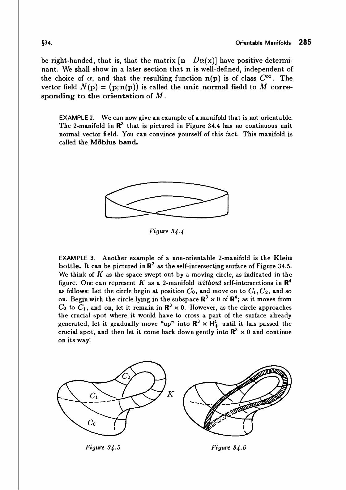
§34. Orientable Manifolds 285
be right-handed , that is, that the matrix [n Da(x)] have positive determinant. We shall show in a later section that n is well-defined, independent of the choice of a, and that the resulting function n(p) is of class coo . The vector field N(p) = (p; n(p)) is called the unit normal field to M corresponding to the orientation of M .
EXAMPLE 2. We can now give an example of a manifold that is not orient able. The 2-manifold in R3 that is pictured in Figure 34.4 has no continuous unit normal vector field. You can convince yourself of this fact. This manifold is called the Mobius band.
Figure 34 .4
EXAM PLE 3. Another example of a non-orientable 2-manifold is the Klein bottle. It can be pictured in R3 as the self-intersecting surface of Figure 34.5. We think of K as the space swept out by a moving circle, as indicated in the figure. One can represent K as a 2-manifold without self-intersections in R4 as follows: Let the circle begin at position Co , and move on to C1 , C2 , and so on. Begin with the circle lying in the subspace R3 x 0 of R\ as it moves from Co to cl ' and on, let it remain in R3 X 0. However' as the circle approaches the crucial spot where it would have to cross a part of the surface already generated, let it gradually move "up" into R3 x H� until it has passed the crucial spot, and then let it come back down gently into R3 x 0 and continue on its way!
](
Figure 34 .5 Figure 34.6

286 Stokes' Theorem Chapter 7
To see that /( is not orientable, we need only note that /( contains a copy of the Mobius band M. See Figure 34.6. If /( were orientable, then M would be orientable as well. (Take all coordinate patches on M that overlap positively the coordinate patches belonging to the orientation of /(.)
Finally, let us consider the case of an n-manifold M in Rn . In this case, not only is M orientable, but it in fact has a "natural" orientation:
Definition. Let M be an n-manifold in Rn . If o: : U --+ V is a coordinate patch on M, then Do: is an n by n matrix. We define the natural orientation of M to consist of all coordinate patches on M for which det Do: > 0 . It is easy to see that two such patches overlap positively.
We must show M may be covered by such coordinate patches. Given p E M , let o: : U --+ V be a coordinate patch about p. Now U is open in either Rn or Hn; by shrinking U if necessary, we can assume that U is either an open €-ball or the intersection with Hn of an open €-ball. In either case, U is connected , so det Do: is either positive or negative on all of U. If the former, then o: is our desired coordinate patch about p; if the latter, then o: o r is our desired coordinate patch about p, where r : Rn --+ Rn is the map
Reversing the orientation of a manifold
Let r : R" --+ R" be the reflection map
it is its own inverse. The map r carries H" to H" if k > 1 , and it carries HI to the left half-line L 1 if k = 1 .
Definition. Let .M be an oriented k-manifold in Rn . If o:; : U; --+ Vi is a coordinate patch on M belonging to the orientation of M , let {3; be the coordinate patch
{3; = o:; o r : r( U; ) --+ V; .
Then {3; overlaps o:; negatively, so it does not belong to the orientation of M. The coordinate patches {3; overlap each other positively, however (as you can check) , so they constitute an orientation of .Af . It is called the reverse, or opposite, orientation to that specified by the coordinate patches o:; .
It follows that every orientable k-manifold M has at least two orientations, a given one and its opposite. If M is connected , it has only two (see

§34. Orientable Manifolds 287
Figure 34. 7
the exercises) . Otherwise , it has more than two. The 1-manifold pictured in Figure 34.7, for example, has four orientations, as indicated .
We remark that if M is an oriented 1-manifold with corresponding tangent field T, then reversing the orientation of M results in replacing T by -T. For if o: : U --+ V is a coordinate patch belonging to the orientation of M , then o: o r belongs to the opposite orientation. Now (o: o r)(t) = o:(-t), so that d(o: o r)fdt = -do:Jdt.
Similarly, if M is an oriented n - 1 manifold in Rn with corresponding normal field N, reversing the orientation of M results in replacing N by -N. For if o: : U --+ V belongs to the orientation of .Af , then o: o r belongs to the opposite orientation . Now
and a(o: o r) ao:
OX; = OX;
Furthermore, one of the frames
ao: (n, a ' xl
ao: . . . ao: ) £lx2 ' ' !lx U U n - 1
and ao:
(-n, - ax. '
if i > 1.
is right-handed if and only if the other one is. Thus if n corresponds to the coordinate patch o:, then -n corresponds to the coordinate patch o: o r.
The induced orientation of aM
Theorem 34.1. Let k > 1 . If M is an orientable k-manifold with non-empty boundary, then aM is orientable.
Proof. Let p E aM; let a : U --+ V be a coordinate patch about p. There is a corresponding coordinate patch a0 on aM that is said to be obtained by restricting o:. (See §24 .) Formally, if we define b : Rl:- l --+ R" by the equation
then a0 = a o b. We show that if a and (J are coordinate patches about p that overlap
positively, then so do their restrictions a0 and (30. Let g : W0 --+ W1 be the
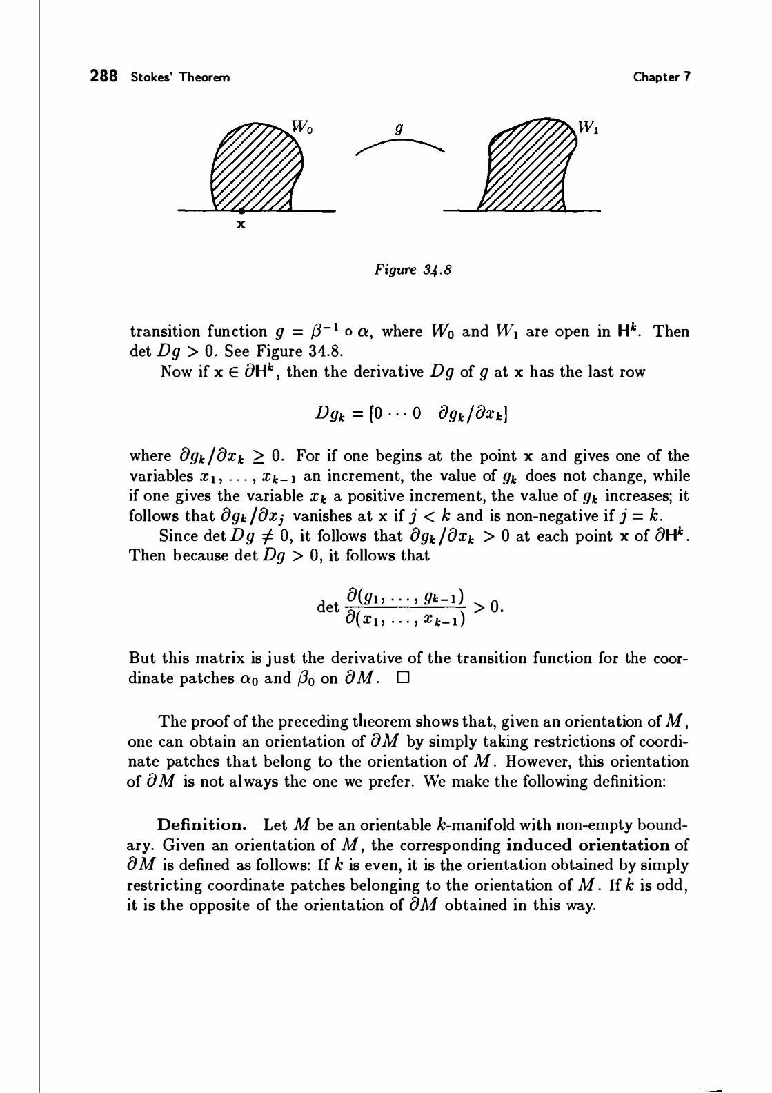
288 Stokes' Theorem Chapter 7
X
Figure 34 .8
transition function g = {J- 1 o a, where W0 and W1 are open in H". Then det Dg > 0. See Figure 34.8.
Now if X E aH" ' then the derivative Dg of g at X has the last row
where agl: I axl: > 0. For if one begins at the point X and gives one of the variables x 1 , . . . , X�:_ 1 an increment, the value of gl: does not change, while if one gives the variable X A: a positive increment, the value of gl: increases; it follows that ag�: laxj vanishes at X if j < k and is non-negative if j = k.
Since det Dg "I 0, it follows that agl: I axl: > 0 at each point X of aH" 0 Then because det Dg > 0, it follows that
d a(g1 , . . . , g�:-d
eta
> 0. (x 1 , . . . , x k_ . )
But this matrix is just the derivative of the transition function for the coordinate patches a0 and (30 on aM. D
The proof of the preceding theorem shows that, given an orientation of M, one can obtain an orientation of aM by simply taking restrictions of coordinate patches that belong to the orientation of M. However, this orientation of aM is not always the one we prefer. We make the following definition:
Definition. Let M be an orientable k-manifold with non-empty boundary. Given an orientation of M, the corresponding induced orientation of aM is defined as follows: If k is even, it is the orientation obtained by simply restricting coordinate patches belonging to the orientation of M . If k is odd , it is the opposite of the orientation of a.Af obtained in this way.

§34. Orientable Manifolds 289
EXAMPLE 4. The 2-sphere S2 and the torus T are orientable 2-manifolds, since each is tbe boundary of a 3-manifold in R3 , which is orient able. In general, if M is a 3-manifold in R3 , oriented naturally, what can we say about the induced orientation of alii? It turns out that it is the orientation of aM that corresponds to the unit normal field to aM pointing outwards from the 3-manifold M. We give an informal argument here to justify this statement, reserving a formal proof until a later section.
Given M, let a : U - V be a coordinate patch on M belonging to the natural orientation of M, about the point p of aM. Then the map
gives the restricted coordinate patch on aM about p. Since dim M = 3, which is odd , the induced orientation of aM is opposite to the one obtained by restricting coordinate patches on 1\f. Thus the normal field N = (p; n) to aM corresponding to tbe induced orientation of M satisfies the condition that tbe frame (-n, aajax1 , aajax2) is right-banded.
On tbe other band, since M is oriented naturally, det Da > 0. It follows that (aajax3 , aajax1 , aajax2) is right-handed. Thus -11 and aajax3 lie on the same side of tbe tangent plane to 1\I at p. Since aajax3 points into M, the vector n points outwards from Af. See Figure 34.9.
Figure 34 .9
,. - - --.... ...... / ' / 8 ' _g_ \ 8..-3 \
' I I
' I \1
EXAMPLE 5. Let M be a 2-manifold with non-empty boundary, in R3 . If M is oriented, let us give aM the induced orientation. Let N be the unit normal field to M corresponding to the orientation of M; and let T be the unit tangent field to aM corresponding to the induced orientation of aM. What is tbe relationship between N and T?

290 Stokes' Theorem Chapter 7
Figure 34 . 10
We assert the following: Given N aud T , for each p E a11f let W(p) be the unit vector that is perpendicular to both N(p) and T(p), chosen so that the frame (N(p) , T(p) , W(p)) is right-handed. Then W(p) is tangent to M at p and points into M from aM.
(This statement is a more precise way of formulating the description usually given in the statement of Stokes' theorem in calculus: "The relation between N and T is such that if you walk around aM in the direction specified by T, with your head pointing in the direction specified by N, then the manifold M is on your left." See Figure 34.1 0.)
To verify this assertion, let a : U - V be a coordinate patch on M about the point p of a111, belonging to tbe orientation of M. Then the coordinate patch a o b belongs to the induced orientation of aM. (Note that dim M = 2, which is even.) The vector aajax1 represents the velocity vector of the parametrized curve a o b; hence by definition it points in tbe same direction as the unit tangent vector T.
The vector aajax2 , on tbe other baud, is the velocity of a parametrized curve that begins at a point p of aM and moves into M as t increases. Thus, by definition, it points into M from p. Now aajax2 need not be orthogonal to M. But we can choose a scalar A such that the vector w =
aajax2 + Aaajaxl is orthogonal to aajax1 and hence to T. Then w also points into M; set W(p) = (p; wj llwll ) .
Finally, the vector N(p) = (p; n) is, by definition, the unit vector normal to M at p such that the frame (n, aajax1 , aajax2) is right-handed. Now
det [n aaj{)x1 aajax2] = det [n aajax1 w] ,
by direct computation. It follows that tbe frame ( N, T, lV) is right-handed.

§34. Orientable Manifolds 291
EXERCISES
1 . Let M be an n-manifold in Rn. Let a , f3 be coordinate patches on M such that det Da > 0 and det D/3 > 0. Show that a and f3 overlap positively if they overlap at all.
2. Let M be a k-manifold in Rn; let a, f3 be coordinate patches on M. Show that if a and f3 overlap positively, so do a o r and f3 o r.
3. Let M be an oriented 1-manifold in R2 , with corresponding unit tangent vector field T. Describe the unit normal field corresponding to the orientation of M.
4. Let C be the cylinder in R3 given by
C = { ( x, y, z) I x2 + y2 = 1 ; 0 < z < 1 } .
Orient C by declaring the coordinate patch a : (0, 1 )2 - C given by
a(u, v) = (cos 21ru, sin 21ru , v)
to belong to the orientation. See Figure 34. 1 1 . Describe the unit normal field corresponding to this orientation of C. Describe the unit tangent field corresponding to the induced orientation of 8C.
v
,... ......... ----..-
c 1-·
u l/
Figure 34 . 1 1
5 . Let M be the 2-manifold i n R2 pictured i n Figure 34.12 , oriented naturally. The induced orientation of aM corresponds to a unit tangent vector field; describe it. The induced orientation of aM also corresponds to a unit normal field; describe it.
6. Show that if M is a connected orientable k-manifold in Rn, then M has precisely two orientations, as follows: Choose an orientation of M; it consists of a collection of coordinate patches {a;} . Let {{3j } be an

292 Stokes Theorem Chapter 7
M
Figure 34 . 1 2
arbitrary orientation of M. Given x E M, choose coordinate patches a; and /3i about X and define A(x) = 1 if they overlap positively at x, and A(x) = -1 if they overlap negatively at x.
(a) Show that A(x) is well-defined, independent of the choice of a; and /3i 0
(b) Show that A is continuous.
(c) Show that A is constant.
(d) Show that {/3i } gives the opposite orientation to {a;} if A is identically -1 , and the same orientation if A is identically 1 .
7. Let M be the 3-manifold in R3 consisting of all x with 1 < l lxll < 2. Orient M naturally. Describe the unit normal field corresponding to the induced orientation of aM.
8 . Let Bn = Bn(I ) be the unit ball in Rn, oriented naturally. Let the unit sphere sn-1 = 8Bn have the induced orientation. Does the coordinate patch a : Int Bn-1 - sn-1 given by the equation
belong to the orientation of sn-1 ? What about the coordinate patch

§35 . Integrating Forms over Oriented Manifolds 293
§35. I NTEGRATING FORMS OVER OR IENTED MAN IFOLDS
Now we define the integral of a k-form w over an oriented k-manifold . The procedure is very similar to that of §25, where we defined the integral of a scalar function over a manifold. Therefore we abbreviate some of the details.
We treat first the case where the support of w can be covered by a single coordinate patch.
Definition. Let M be a compact oriented k-manifold in Rn . Let w be a k-form defined in an open set of Rn containing M . Let C = M n(Support w) ; then C is compact. Suppose there is a coordinate patch a : U --+ V on M belonging to the orientation of .M such that C C V. By replacing U by a smaller open set if necessary, we can assume that U is bounded. We define the integral of w over M by the equation
1 - 1 ..
w - a w. M Int U
Here Int U = U if U is open in Rk, and Int U = U n H� if U is open in Hk but not in Rk .
First , we note that this integral exists as an ordinary integral , and hence as an extended integral : Since a can be extended to a coo map defined on a set U' open in Rk, the form a• w can be extended to a coo form on U'. This form can be written as h dx1 A · · · A dx k for some coo scalar function h on U' . Thus 1 .. - 1 h a w - , lnt U Int U by definition. The function h is continuous on U and vanishes on U outside the compact set a- 1 (C); hence h is bounded on U. If U is open in Rk , then h vanishes near each point of Bd U. If U is not open in Rk , then h vanishes near each point of Bd U not in 8Hk , a set that has measure zero in Rk . In either case, h is integrable over U and hence over Int U. See Figure 35 . 1 .
Second, we note that the integral JM w is well-defined, independent of the choice of the coordinate patch a . The proof is very similar to that of Lemma 25. 1 ; here one uses the additional fact that the transition function is orientation-preserving, so that the sign in the formula given in Theorem 33.1 is "plus."

294 Stokes' Theorem
Figure 35. 1
Chapter 7
u
\ \ I I I a - ' / - - ...... - _..,. *"'
Third , we note that this integral is linear. More precisely, if w and 'f/ have supports whose intersections with M can be covered by the single coordinate patch a : U --+ V be longing to the orientation of M, then
f aw + b'f/ lu a f w lu + b [ 'f/· 11\f
This result follows at once fwm the fact that a" and .hnt u are linear. Finally, we note that if -M denotes the manifold M with the opposite
orientation, then 1 w = - [ w . -M jM
This result follows from Theorem 33 . 1 . To define JM w in general , we use a partition of unity.
Definition. Let M be a compact oriented k-manifold in Rn . Let w be a k-form defined in an open set of Rn containing M. Cover M by coordinate patches be longing to the orientation of .Af; then choose a partition of unity </>, . . . , <f>t on M that is dominated by this collection of coordinate patches on M. See Lemma 25.2. \Ve define the integral ofw over M by the equation
l 1 w = L[l <f>;w] . M i = l M

§35. Integrating Forms over Oriented Manifolds 295
The fact that this definition agrees with the previous one when the support of w is covered by a single coordinate patch follows from linearity of the earlier integral and the fact that
l w(x) = L </>;(x)w(x)
i = l for each x E M. The fact that the integral is independent of the choice of the partition of unity follows by the same argument that was used for the integral JM f d V. The following is also immediate:
Theorem 35. 1. Let M be a compact oriented k-manifold in Rn . Let w, 'f/ be k-forms defined in an open se t of Rn containing M. Then
L (aw + b'f/) a JM w + b L 'f/·
If -M denotes M with the opposite orientation, then
1 w = - { w. D -M jM
This definition of the integral is satisfactory for theoretical purposes, but not for computational purposes. As in the case of the integral JM f dV, the practical way of evaluating JM w is to break M up into pieces, integrate over each piece separately, and add the resu lts together. We state this fact formally as a theorem:
*Theorem 35.2. Let M be a compact oriented k-manifold in Rn . Let w be a k-form defined in an open set of Rn containing M. Suppose that a; : A; --+ M;, for i = 1 , . . . , N, is a coordinate patch on M belonging to the orientation of M, such that A; is open in Rk and M is the disjoint union of the open sets M1 , . . . , MN of M and a se t [( of measure zero in M. Then
Proof. The proof is almost a copy of the proof of Theorem 25.4. Alternatively, it follows from Theorems 25.4 and 36.2. We leave the details to you. D

296 Stokes' Theorem Chapter 7
EXERCIS ES
1 . Let M be a compact oriented k-manifold in R". Let w be a k-form defined in an open set of R" containing M.
(a) Show that in the case where the set C = M n (Support w) is covered by a single coordinate patch, the integral JM w is well-defined.
(b) Show that the integral JM w is well-defined in general, independent of the choice of the partition of unity.
2. Prove Theorem 35.2. 3. Let sn-l be the unit sphere in R"' oriented so that the Coordinate patch
a : A - S"-1 given by
belongs to the orientation, where A = lnt B"-1 • Let 7J be the n - 1 form
n 7] = L (-l) i- If; dX I f\ . . . f\ d;; f\ . . . 1\ dxn,
i=: 1
where f; (x) = x;j llxllm · The form 7J is defined on R" - 0. Show that
as follows:
(a) Let p : R" ---+ R" be given by
p(xl ' . . . ' Xn-1 ' Xn) = (xi ' . . . ' Xn-1 ' -Xn) ·
Let f3 = p o a. Show that f3 : A -- S"-1 belongs to the opposite orientation of S"-1 • [Hint: The map p : B" - B" is orientationreversing.)
(b) Show that /3* 7] = -a•
7J; conclude that
(c) Show that
r 7] = 2 r a•
7J. Jsn-l }A

§36. A Geometric Interpretation of Forms and Integrals 297
*§36. A G EOM ETRIC I NTERPRETATIO N OF FORMS AND INTEGRALS
The notion of the integral of a k-form over an oriented k-manifold seems remarkably abstract. Can one give it any intuitive meaning? We discuss here how it is related to the integral of a scalar function over a manifold , which is a notion closer to our geometric intuition.
First, we explore the relationship between alternating tensors in Rn and the volume function in Rn .
Theorem 36.1. Let W be a k-dimensional linear subspace of Rn; le t ( a1 , . . . , ak ) be an orthonormal k-frame in W, and le t f be an alternating k-tensor on W. If (xt , . . . , Xk) is an arbitrary k-tuple in W, then
f(xt , . . . , xk) = E V(xt , . . . , xk)f(at , . . . , ak ) ,
where E = ± 1 . If the Xi are independent, then E = + 1 if the frames (x1 , . . . , Xk ) and (a1 , . . . , ak ) belong to the same orientation of W and E = - 1 otherwise.
If the Xi are dependent, then V ( Xt , . . . , Xk ) = 0 by Theorem 21 .3 and the value of E does not matter.
Proof. Step 1. If W = Rk , then the theorem holds. In that case, the k-tensor f is a multiple of the determinant function, so there is a scalar c such that for all k-tuples (xt , . . . , Xk ) in Rk ,
f(x t , . . . , Xk ) = cdet[xt · · · Xk]·
If the x; are dependent, it follows that f vanishes; then the theorem holds trivially. Otherwise, we have
where E1 = +1 if (x1 , . . . , xk ) is right-handed, and E1 = - 1 otherwise. Similarly,
f(al , . . . , ak) = CE2V(a1 , . . . , ak ) = CE2 ,
where E2 + 1 if (at , . . . , ak) is right-handed and E2 = -1 otherwise. It follows that
where Et /E2 = +1 if (x1 , . . . , Xk ) and (at , . . . , ak ) belong to the same orientation of Rk , and E 1 / E 2 = - 1 otherwise .

298 Stokes' Theorem Chapter 7
Step 2. The theorem holds in general. Given W, choose an orthogonal transformation h : Rn --+ Rn carrying W onto Rk X 0. Let k : Rk X 0 --+ W be the inverse map. Since f is an alternating tensor on W, it is mapped to an alternating tensor k• f on Rk X 0 . Since (h(x1 ), . . . , h(xk )) is a k-tuple in Rk X 0, and (h(a! ), . . . , h(ak )) is an orthonormal k-tuple in Rk X O, we have by Step 1 ,
(k* f) (h(x! ) , . . . , h(xk )) = �: V (h(x! ) , . . . , h(xk )) (k* f) (h(a! ) , . . . , h(ak )) ,
where E = ±1. Since V is unchanged by orthogonal transformations, we can rewrite this equation as
as desired . Now suppose the x; are independent. Then the h(x; ) are independent, and by Step 1 we have E = + 1 if and only if (h(x1 ) , . . . , h (xk )) and ( h( a1 ) , . . . , h( ak )) belong to the same orientation of Rk X 0. By definition, this occurs if and only if ( x1 , . . . , Xk ) and (a� , . . . , ak ) belong to the same orientation of W. D
Note that it follows from this theorem that if (a1 , . . . , ak) and (bh . . . , bk ) are two orthonormal frames in W, then
the sign depending on whether they belong to the same orientation of W or not.
Definition. Let M be a k-manifold in Rn ; let p E M. If M is oriented, then the tangent space to M at p has a natural induced orientation, defined as follows: Choose a coordinate patch a : U --+ V belonging to the orientation of M about p. Let a(x) = p. The collection of all k-frames in Tp( M) of the form
(a. (x; ai ), . . . , a. (x; ak )) where ( a1 , . . . , ak ) is a right-handed frame in R" , is called the natural orientation of Tp (M ) , induced by the orientation of M. It is easy to show it is well-defined, independent of the choice of a.
Theorem 36.2. Let M be a compact oriented k-manifold in Rn ; let w be a k-form defined in an open set of Rn containing M. Let A be the scalar function on M defined by the equation
A (p) = w(p) ( (p ; a! ), . . . , (p; ak )) ,
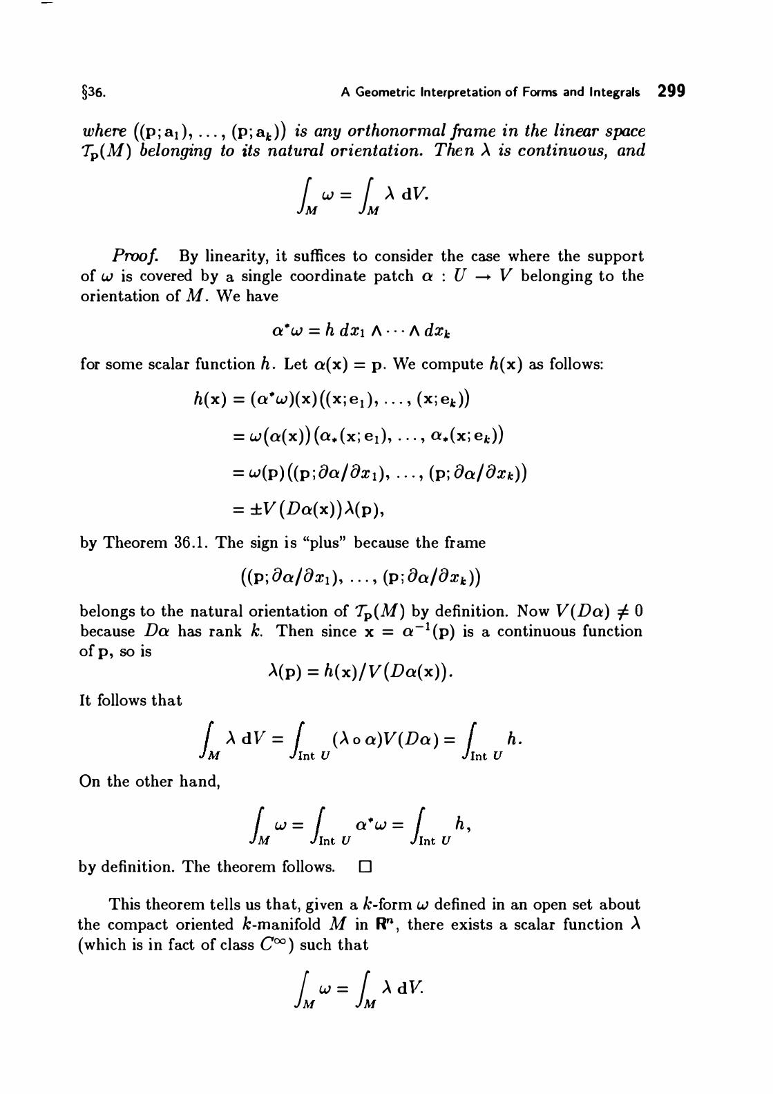
§36. A Geometric Interpretation of Forms and Integrals 299
where ((p ; ad, . . . , (p; aA: )) is any orthonormal frame in the linear space Tp(M) belonging to its natural orientation. Then A is continuous, and
L w = L A dV.
Proof. By linearity, it suffices to consider the case where the support of w is covered by a single coordinate patch a : U --+ V belonging to the orientation of M. We have
a"w = h dx1 A . · · A dx�: for some scalar function h . Let a(x) = p. We compute h(x) as follows:
h(x) = (a"w)(x) ((x ; ed, . . . , (x ; e�: ))
= w(a(x)) (a,. (x ; ed, . . . , a,. (x ; e�:))
= w(p) ((p ; aafaxi ) , . . . , (p; aafax�:))
= ±V (Da(x)) A(p), by Theorem 36. 1 . The sign is "plus" because the frame
((p; aafaxi ) , . . . , (p ; aafax�: )) belongs to the natural orientation of Tp(M) by definition. Now V(Da) "I 0 because Da has rank k. Then since x = a-1 (p) is a continuous function of p, so is
It follows that
A(p) = h(x)/V(Da(x)) .
f A dV = f (A o a)V(Da) = f h . 1M lint U lint U
On the other hand,
f w = f a"w = f h , 1M lint U lint U
by definition. The theorem follows. D
This theorem tells us that, given a k-form w defined in an open set about the compact oriented k-manifold M in Rn , there exists a scalar function A (which is in fact of class C00 ) such that
jM
w = L A dY

300 Stokes' Theorem Chapter 7
The reverse is also true, but the proof is a good deal harder: One first shows that there exists a k-form Wv , defined in an open set
about M, such that the value of Wv (p) on any orthonormal basis for Tp( M) belonging to its natural orientation is 1 . Then if A is any C00 function on M, we have
thus the integral of A over M can be interpreted as the integral over M of the form AWv . The form Wv is called a volume form for M, since
This argument applies, however , only if .Af is orientable. If M is not orientable, the integral of a scalar function is defined, but the integral of a form is not.
A remark on notation. Some mathematicians denote the volume form Wv by the symbol dV, or rather by the symbol dV. (See the remark on notation in §22.) While it makes the preceding equations tautologies, this practice can cause confusion to the unwary, since V is not a form, and d does not denote the differential operator in this context !
EXERCIS E
1 . Let M be a k-manifold in Rn; let p E M. Let a and f3 be coord inate patches on Af about p; let a(x) = p = f3(y) . Let (a1 , • • • , ak ) be a right-handed frame in Rk . If a and f3 overlap positively, show that there is a right-handed frame (b1 , . . . , bk) in Rk such that
a. (x; a; ) = {3. (y; b;)
for each i. Conclude that if Af is oriented , then the natural orientation of Tp(M) is well-defined.

§37. The Generalized Stokes' Theorem 301
§37. THE GEN ERALIZED STOKES ' THEOREM
Now, finally, we come to the theorem that i s the culmination of all our labors. It is a general theorem about integrals of differential forms that includes the three basic theorems of vector integral calculus-Green's theorem, Stokes' theorem, and the divergence theorem-as special cases.
We begin with a lemma that is in some sense a very special case of the theorem. Let Jk denote the unit k-cube in R" ;
I" = [0 , 1]" = [0, 1] X 0 0 0 X [0, 1] .
Then lnt I" is the open cube (0, 1 )" , and Bd I" equals Ik - lnt I" .
Lemma 37.1. Let k > 1 . Let 'f/ be a k - 1 form defined in an open set U of Rk containing the unit k-cube I" . Assume that 'f/ vanishes at all points of Bd Ik except possibly at points of the subset (Int I" - 1 ) x 0. Then
[ d'f/ = ( -1)k [ b*'f/, lint Jk lint Jk-1
where b : I"- 1 -+ Jk is the map
Proof. We use x to denote the general point of Rk , and u to denote the general point of Rk- 1 . See Figure 37 . 1 . Given j with 1 < j < k, Jet Ii denote the k - 1 tuple
Ii = ( 1 , . . . , ), . . . , k ) .
Then the typical elementary k - 1 form in Rk i s the form
-
Because the integrals involved are linear and the operators d and b• are linear, it suffices to prove the lemma in the special case
so we assume this value of 'f/ in the remainder of the proof.
Step 1 . We compute the integral
[ d,. lint Jk

302 Stokes' Theorem
I u
Figure 37.1
We have
k = ( L D;J dx;) A dx1;
i=1
Then we compute
f d'f/ = (-1)i-1 f Dif lint Jk lint Jk
= (-1 )i- 1 f Di f l[k
Chapter 7
Support 7J
by the Fubini theorem, where v = (x1 , . . . , Xj , . . . , Xk ) · Using the fundamental theorem of calculus, we compute the inner integral as
1 Di f(x� , . . . , xk) = f(x� , . . . , 1 , . . . , xk ) - j(x 1 , . . . , 0, . . . , xk ), z; ; E l
where the 1 and the 0 appear in the ph place. Now the form 'f/, and hence the function f, vanish at all points of Bd [k except possibly at points of the open bottom face (Int Jk-1 ) X 0. If j < k, this means that the right side of this equation vanishes; while if j = k, it equals
-f(x� , . . . , Xk- 1 , 0) .

§37. The Generalized Stokes' Theorem 303
We conclude the following :
f d'f/ = lint Jk
0 if j < k,
(- 1)" J[k -l (f 0 b) if j = k.
Step 2. Now we compute the other integral of our theorem. The map b : R"- 1 -+ R" has derivative [h-1 ] Db = .
0
Therefore , by Theorem 32 .2, we have
b• (dxi; ) = (det Db(1 , . . . , ), . . . , k)] du1 A · · · A dul:-1
We conclude that
f b·, = lint Jk-1
0
if j < k, if j = k.
if j < k,
hnt [k-1 (/ o b) if j = k.
The theorem follows by comparing this equation with that at the end of Step 1 . D
Theorem 37.2 (Stokes' theorem). Let k > 1 . Let M be a compact oriented k-manifold in Rn; give {}M the induced orientation if {} M is not empty. Let w be a k - 1 form defined in an open se t of Rncontaining M. Then
JM dw = laM W
if {}M is not empty; and JM dw = 0 if {}M is empty.
Proof. Step 1. We first cover M by carefully-chosen coordinate patches. As a first case, assume that p E M - {} M. Choose a coordinate patch a : U -+ V belonging to the orientation of M, such that U is open in R" and contains the unit cube Jl: , and such that a carries a point of lnt Jl: to the point p . (If we begin with an arbitrary coordinate patch a : U -+ V about p belonging to the orientation of .Af, we can obtain one of the desired type by preceding a by a translation and a stretching in R" .) Let W = Int Jl: ,

304 Stokes' Theorem
w
" - - ...,,
Figure 37.2
I I
Chapter 7
w
/
and let Y = a(lV). Then the map a : W ---> Y is still a coordinate patch be longing to the orientation of M about p , with W = Int Jk open in Rk . See Figure 37.2. We choose this special patch about p .
As a second case, assume that p E 8111 . Choose a co ordinate patch a : U ---> V be longing to the orientation of .Af , such that U is open in Hk and U contains [k , and such that a carries a point of ( Int [k- l ) X 0 to the point p . Let
W = (lnt Jk) U ((Int [k- l ) X 0) ,
and let Y = a(W). Then the map a : W ---> Y is still a coordinate patch be longing to the orientation of M about p, with W open in Hk but not open in Rk .
We shall use the covering of M by the coordinate patches a : W ---> Y to compute the integrals involved in the theorem. Note that in each case, the map a can be extended if necessary to a coo function defined on an open set of Rk containing [k .
Step 2. Since the operator d and the integrals involved are linear, it suffices to prove the theorem in the special case where w is a k - 1 form such that the set
C = M n (Support w)
can be covered by a single one of the coordinate patches a : W ___. Y. Since the support of dw is contained in the support of w, the set M n (Support dw) is contained in C, so it is covered by the same coordinate patch.
Let 'f/ denote the form a"w. The form 'f/ can be extended if necessary (without change of notation) to a C00 form on an open set ofRk containing [k .
§37. The Generalized Stokes' Theorem 305
Furthermore, 'f/ vanishes at all points of Bd Jk except possibly at points of the bottom face (Int Jk- 1 ) x 0. Thus the hypotheses of the preceding lemma are satisfied.
Step 3. We prove the theorem when C is covered by a coordinate patch a : W ___. Y of the type constructed in the first case. Here W = Int Jk and Y is disjoint from {} M. We compute the integrals involved . Since a• dw = da*w = d'f/, we have
f dw = f a*dw = f d'f/ = (-l)k f b*'f/· 1M lint Jk lint Jk lint Jk- 1
Here we use the preceding lemma. In this case, the form 'f/ vanishes outside Int Jk . In particular, 'f/ vanishes on Jk- 1 X 0, so that b* 'f/ = 0. Then JM dw = 0.
The theorem follows. If {} M is empty, this is the equation we wished to prove. If {} M is non-empty, then the equation
f dw = f w 1M laM
holds trivially; for since the support of w is disjoint from {} M, the integral of w over {} M vanishes.
Step 4· Now we prove the theorem when C is covered by a coordinate patch a : W ___. Y of the type constructed in the second case. Here W is open in Hk but not in Rk , and Y intersects {} .Af . We have Int W = Int Jk . We compute as before
f dw = f d'f/ = (-l)k f b*'f/. 1M lint Jk lint Jk- l
We next compute the integral JaM w. The set {}.Af n (Support w) is covered by the coordinate patch
(J = a o b : Int Jk-1 ___. Y n {}M
on {} M, which is obtained by restricting a. Now (J belongs to the induced orientation of {}M if k is even, and to the opposite orientation if k is odd. If we use (J to compute the integral of w over {} .Af, we must reverse the sign of the integral when k is odd. Thus we have
f w = (- l)k f (J*w. laM lint Jk- l
Since (J•w = b*(a*w) = b*'f/, the theorem follows. D
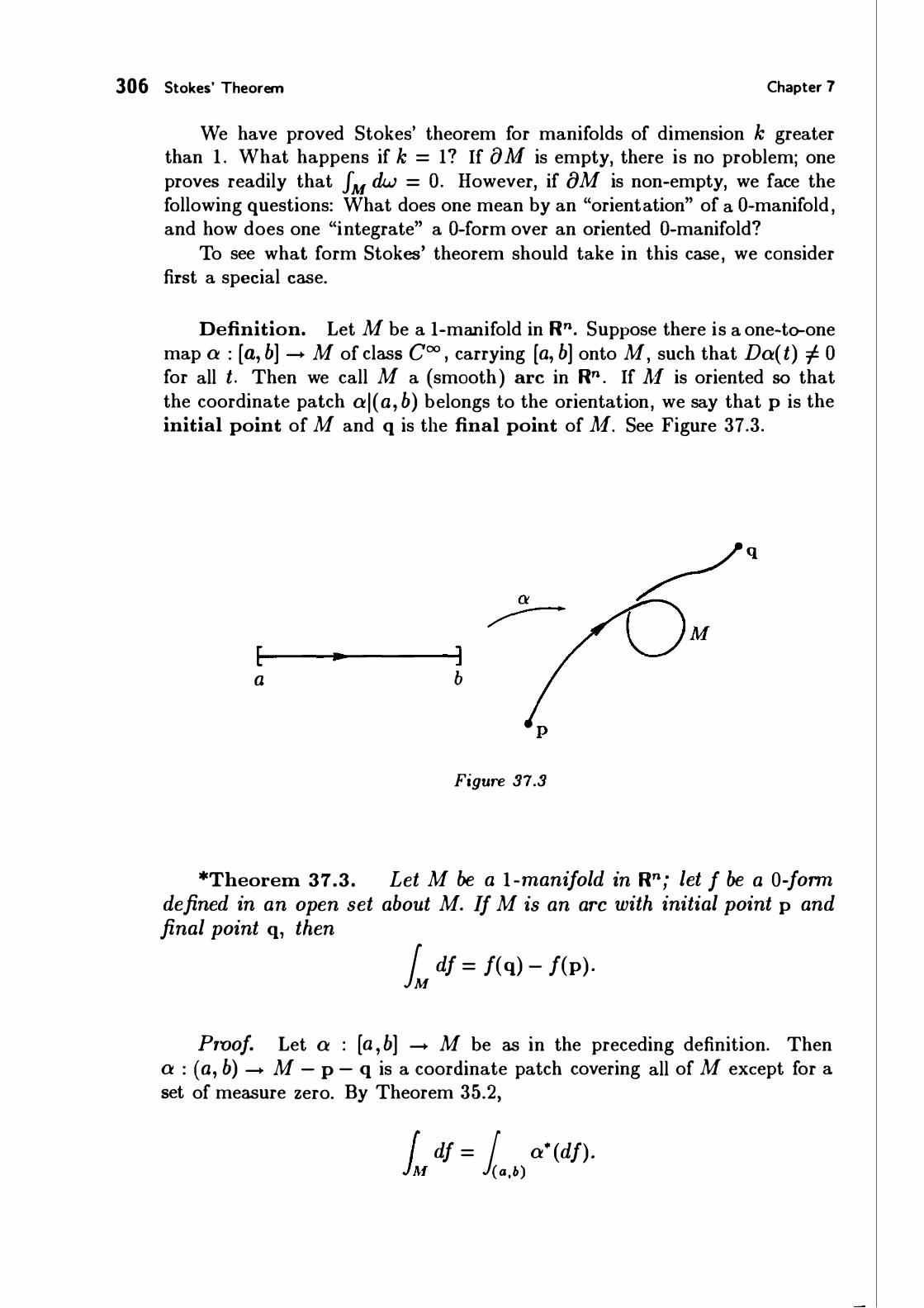
306 Stokes' Theorem Chapter 7
We have proved Stokes' theorem for manifolds of dimension k greater than 1 . What happens if k = 1? If {} .Af is empty, there is no problem; one proves readily that JM dw = 0. However, if {}M is non-empty, we face the following questions: What does one mean by an "orientation" of a 0-manifold , and how does one "integrate" a 0-form over an oriented 0-manifold?
To see what form Stokes' theorem should take in this case, we consider first a special case.
Definition. Let M be a 1-manifold in Rn. Suppose there is a one-to-one map a : [a, b] -+ M of class coo , carrying [a, b] onto M, such that Da(t) "I 0 for all t. Then we call M a (smooth ) arc in Rn . If Af is oriented so that the coordinate patch al(a, b) belongs to the orientation, we say that p is the initial point of M and q is the final point of .M. See Figure 37.3.
q
[ .. ] a b
Figure 37.3
*Theorem 37.3. Let M be a ! -manifold in Rn; let f be a 0-form defined in an open set about M. If M is an arc with initial point p and final point q, then
L df = f(q) - f(p) .
Proof. Let a : [a , b] -+ M be as in the preceding definition. Then a : (a, b) -+ M - p - q is a coordinate patch covering all of M except for a set of measure zero. By Theorem 35.2,
{ df = j a* (df). JM (a,b)

§37. The Generalized Stokes' Theorem 307
Now a* (df) = d(f o a) = D(f o a) dt,
where t denotes the general point of R. Then
1 a*(df) = 1 D(f o a) = f(a(b)) - f(a(a)) , (a,b) (a,b)
by the fundamental theorem of calculus. D
This result provides a guide for formulating Stokes' theorem for 1-manifolds:
Definition. A compact 0-manifold N in Rn is a finite collection of points {XI , . . . , Xm } of Rn. We define an orientation of N to be a function f. mapping N into the two-point set { -1 , 1 } . If f is a 0-form defined in an open set of Rn containing N, we define the integral of f over the oriented manifold N by the equation
m 1 f = L E(x;)/(x;) . N i=l
Definition. If M is an oriented 1-manifold in Rn with non-empty boundary, we define the induced orientation of {} M by setting f.(p) = -1 , for p E aM, if there is a coordinate patch a : U -+ V on M about p belonging to the orientation of M, with U open in W . We set E(p) = + 1 otherwise . See Figure 37 .4.
0 (. = -1
Figure 37.4
(. = +1
._ I 0
With these definitions, Stokes' theorem takes the following form; the proof is left as an exercise.

308 Stokes' Theorem Chapter 7
Theorem 37.4 (Stokes' theorem in dimension 1). Let M be a compact oriented !-manifold in Rn; give {}M the induced orientation if {}M is not empty. Let f be a 0-form defined in an open set of Rn containing M. Then
L df = JaM !
if {}M is not empty; and JM df = 0 if {}M is empty. D
EXERCIS ES
1 . Prove Stokes' theorem for !-manifolds. [Hint: Cover M by coordinate patches, belonging to the orientation of Af, of the form a : W -+ Y, where W is one of the intervals (0,1) or [0, 1) or (- 1 ,0). Prove the theorem when the set A-1 n (Support f) is covered by one of these coordinate patches.)
2. Suppose there is an n - 1 form 7J defined in Rn - 0 such that d7] = 0 and
Show that 7J is not exact. (For the existence of such an 7], see the exercises of §30 and the exercises of either §35 or §38.)
3. Prove the followi ng:
Theorem (Gl'een's thcm·em) . Let M be a compact 2-manifold in R2 , o riented naturally; give {)Af the induced orientation. Let P dx + Q dy be a ! -form defined in an open set of R2 about M. Th en
4. Let M be the 2-manifold in R3 consisting of all points x such that
Then {)J\1 is the circle consisting of all points such that
See Figure 37.5. The map
for u2 + v2 < 1 , is a coordinate patch on M that covers M - {)M. Orient M so that a belongs to the orientation, and give {)M the i nduced orientation.

§37.
/ /
I ' I I I
)-
Figure 37.5
The Generalized Stokes' Theorem 309
(a) What normal vector corresponds to the orientation of M? What tangent vector corresponds to the induced orientation of aM?
(b) Let w be the 1-form w = X2 dx1 + 3xl dx3 . Evaluate faM w directly.
(c) Evaluate Jllf dw directly, by expressing it as an integral over the unit disc in the �u, v) plane.
5. The 3-ball B3(r) is a 3-manifold in R3 ; orient it naturally and give S2(r) the induced orientation. Assume that w is a 2-form defined in R3 - 0 such that
for each r > 0 .
1 w = a + (b/r) , S2(r)
(a) Given 0 < c < d, let 111 be the 3-manifold in R3 consisting of all x with c < l lxl l < d, oriented naturally. Evaluate J M dw.
(b) If dw = 0 , what can you say about a and b?
(c) If w = dry for some ry in R3 - 0 , what can you say about a and b?
6. Let M be an oriented k + l + 1 manifold without boundary in Rn. Let w be a k-form and let ry be an £-form, both defined in an open set of Rn about M. Show that
L w A dry = a L dw A ry
for some a, and determine a.

31 0 Stokes' Theorem Chapter 7
*§38. AP PL ICATIONS TO VECTOR ANALYSIS
In general, we know from the discussion in §31 that differential forms of order k can be interpreted in Rn in certain cases as scalar or vector fields, namely when k = 0, 1 , n - 1 , or n. We show here that integrals of forms can similarly be so interpreted; then Stokes' theorem can also in certain cases be interpreted in terms of scalar or vector fields. These versions of the general Stokes' theorem include the classical theorems of the vector integral calculus.
We consider the various cases one-by-one.
The gradient theorem for 1-manifolds in Rn
First , we interpret the integral of a 1-form in terms of vector fields. If F is a vector field defined in an open set of Rn , then F corresponds under the "translation map" a 1 to a certain 1-form w. (See Theorem 31 . 1 . ) It turns out that the integral of w over an oriented 1-manifold equals the integral , with respect to 1-volume, of the tangential component of the vector field F. That is the substance of the following lemma:
Lemma 38.1. Let M be a compact oriented ! -manifold in Rn; let T be the unit tangent vector to M corresponding to the orientation. Let
F(x) = (x ; f(x)) = (x; Ef; (x)e;) be a vector field defined in an open set of Rn containing M; it corresponds to the 1 -form
w = I: f; dx; . Then
f w = f {F, T) ds. 11\f 11\f
Here we use the classical notation "ds" rather than "d V" to denote the integral with respect to 1-volume (arc length) , simply to make our theorems resemble more closely the classical theorems of vector integral calculus.
Note that if one replaces M by - Jo.,f, then the integral JM w changes sign. This replacement has the effect of replacing T by -T; thus the integral JM (F, T) ds also changes sign.
Proof. We give two proofs of this lemma. The first relies on the results of §36; the second does not .
First proof. By Theorem 36.2, we have
JM
W = JM
..\ ds,

§38. Applications to Vector Analysis 311
where ..\(p) is the value of w(p) on an orthonormal basis for Tp(M) that belongs to the natural orientation of this tangent space. In the present case, the tangent space is !-dimensional, and T(p) is such an orthonormal basis. Let T(p) = (p; t) . Since w = Ej; dx; ,
w(p) (p; t) = :L:J;(p)t; (p) . Thus
..\(p) = {F(p) , T(p)) , and the lemma follows.
Second proof. Since the integrals involved are linear in w and F, respectively, it suffices to prove the lemma in the case where the set
C = Af n (Support w) lies in a single coordinate patch a : U ----> V belonging to the orientation of M. In that case, we simply compute both integrals. Let t denote the general point of R. Then
n
a*w = I: (f; o a) da; i=l
n
= L (f; o a) (Da;) dt i=l
= {f o a, Da) dt. It follows that
f w = f a*w JM lrnt u
= f {f o a, Da) . lrnt u
On the other hand,
smce
f {F, T) ds = f (F o a , T o a) · V(Da) JM lrnt u
= f {f o a, Da/ I IDall ) · V(Da) lrnt u
= f {f o a, Da) , lrnt u
V(Da) = [det(Da tr · Da)]112 = I IDall · The lemma follows. 0

312 Stokes' Theorem Chapter 7
Theorem 38.2 (The gradient theorem). Let M be a compact !-manifold in Rn; let T be a unit tangent vector field to M. Let f be a coo function defined in an open set about M. If 8M is empty, then
JM {grad f, T) ds = 0.
If 8M consists of the points x1 , . . . , xm , let €; = -1 if T points into M at x; and €; = +1 otherwise. Then
m 1 {grad f, T) ds = L E; j(x;) . M i: 1
Proof. The 1-form df corresponds to the vector field grad f, by Theorem 3 1 . 1 . Therefore
f df = f {grad f, T) ds, jM jM by the preceding lemma. Our theorem then follows from the !-dimensional version of Stokes' theorem. 0
The divergence theorem for n-1 manifolds in Rn
Now we interpret the integral of an n - 1 form, over an oriented n - 1 manifold M, in terms of vector fields. First, we must verify a result stated earlier, the fact that an orientation of M determines a unit normal vector field to M. Recall the following definition from §34:
Definition. Let M be an oriented n - 1 manifold in Rn. Given p E M, let (p; n) be a unit vector in Tp(Rn) that is orthogonal to the n- 1 dimensional linear subspace Tp(M). If a : U --+ V is a coordinate patch on M about p belonging to the orientation of M with a (x) = p, choose n so that
8a 8a (n, 8
(x), . . · , 8
(x)) X1 Xn- 1
is right-handed . The vector field N (p) = (p; n(p)) is called the unit normal field corresponding to the orientation of M.
We show N (p) is well-defined, and of class C00 • To show it is well-defined, let {3 be another coordinate patch about p, belonging to the orientation of M. Let g = {3-1 o a be the transition function, and let g(x) = y. Since a = {3 o g,
Da(x) = D{3(y) · Dg(x).

§38. Applications to Vector Analysis 313
Then for any v E Rn, we have the equation
[v Da(x)] = [v D,B(y)] 1 0
0 Dg(x) •
(Here Da and D,B have size n by n - 1 , so each of these three matrices has size n by n .) It follows that
det[v Da(x)] = det[v D,B(y)] · det Dg(x) .
Since det Dg > 0, we conclude that [v Da(x)] has positive determinant if and only if [v D,B(y)] does.
To show that N is of class C00 , we obtain a formula for it. As motivation, let us consider the case n = 3:
EXAMPLE 1 . Given two vectors a and b in R3, one learns in calculus that their cross product c = a x b is perpendicular to both, that the frame ( c, a, b) is right-handed, and that l lc l l equals V(a, b). The vector c is, of course, the vector with components
It follows that if M is an oriented 2-m ani fold in R3 , and if a : U --+ V is a coordinate patch on A1 belonging to the orientation of A1, and if we set
aa aa C
= fJx1 X fJx2 '
then the vector n = c/ l lc l l gives the corresponding unit normal to M. See Figure 38.1 .
X u
Figure 38. 1

314 Stokes' Theorem Chapter 7
There is a formula similar to the cross product formula for determining n
in general, as we now show.
Lemma 38.3. Given independent vectors x 1 , . . . , Xn- 1 in Rn, let X be the n by n - 1 matrix X = [x 1 · · · Xn_ 1] , and let c be the vector c = Ec;e; , where
c; = (-1)i- 1 det X(1 , . . . , T, . . . , n) . The vector c has the following properties:
( 1) c is non-zero and orthogonal to each x; . (2) The frame ( c, xu . . . , Xn- I ) is right-handed. (3) l lcl l = V(X) . Proof. We begin with a preliminary calculation. Let x1 , . . . , Xn- 1 be
fixed. Given a E Rn , we compute the following determinant; expanding by cofactors of the first column, we have :
n det [a X1 · · · Xn-d = I: a; ( -1)i- 1 det X(l , . . . , T, . . . , n)
i: 1
= (a, c) . This equation contains all that is needed to prove the theorem.
(1) Set a = X; . Then the matrix [a X1 · · · Xn-1] has two identical columns, so its determinant vanishes. Thus {x; , c) = 0 for all i , so c is orthogonal to each x; . To show c =/= 0 , we note that since the columns of X span a space of dimension n - 1 , so do the rows of X. Hence some set consisting of n - 1 rows of X is independent , say the set consisting of all rows but the ith . Then c; =/= 0; whence c =/= 0.
(2) Set a = c. Then
det [c X1 · · · Xn- 1] = (c, c) = l l cW > 0 .
Thus the frame ( c , Xu . . . , Xn-d is right-handed. (3) This equation follows at once from Theorem 21 .4 . Alternatively, one
can compute the matrix product
[c X1 · · · Xn-dtr · [c X1 · · · Xn- 1] = 0
0 Xtr · X Taking determinants and using the formula in (2), we have
l l cl l4 = l l c i i 2V(X)2 • Since l l c l l =/= 0, we conclude that l l cl l = V(X). 0
•

§38. Applications to Vector Analysis 315
Corollary 38.4. If M is an oriented n - 1 manifold in Rn , then the unit normal vector N (p) corresponding to the orientation of M is a coo function of p.
Proof. If a : U ----> V is a coordinate patch on M about p, let
c; (x) = ( -1)i- l det Da(1 , . . . , z, . . . , n)(x)
for x E U, and let c(x) = Ec;(x)e; . Then for all p E V, we have
N(p) = (p; c(x)/ l lc(x) l l ) ,
where x = a- 1 (p ) ; this function is of class coo as a function of p. 0
Now we interpret the integral of an n - 1 form in terms of vector fields. If G is a vector field in Rn, then G corresponds under the "translation map" f3n- 1 to a certain n - 1 form w in Rn. (See Theorem 31 . 1 .) It turns out that the integral of w over an oriented n -1 manifold M equals the integral over M, with respect to volume, of the normal component of the vector field G. That is the substance of the following lemma:
Lemma 38.5. Let M be a compact oriented n - 1 manifold in Rn; let N be the corresponding unit normal vector field. Let G be a vector field defined in an open set U of Rn containing M. If we denote the geneml point of Rn by y, this vector field has the form
G(y) = (y; g(y)) = (y; Eg; (y)e;) ;
it corresponds to the n - 1 form
n w = :L: (-1) i- 1g; dy1 A . . · A dY; A . . · A dYn ·
i: l Then
L w = JM
{G, N) dV.
Note that if we replace M by -.M , then the integral JM w changes sign. This replacement has the effect of replacing N by -N, so that the integral JM(G, N) dV also changes sign.
Proof. We give two proofs of this theorem. The first relies on the results of §36 and the second does not.

316 Stokes' Theorem
First proof. By Theorem 36.2, we have
Chapter 7
where ..\(p) is the value of w(p) on an orthonormal basis for Tp( M) that belongs to the natural orientation of this tangent space. We show that >. = {G, N), and the proof is complete .
Let (p; al ) , . . . , (p; an-d be an orthonormal basis for Tp(M) that belongs to its natural orientation. Let A be the matrix A = [a1 · · · an- 1] ; and let c be the vector c = Ec;e;, where
. I � c; = (-1)'- det A( l , . . . , z, . . . , n) .
By the preceding lemma, the vector c is orthogonal to each a; , and the frame (c , au . . . , an-d is right-handed , and
l l c l l = V(A) = [det(Atr · A)] 112 = [det ln- 1] 1 12 = 1 .
Then N = (p; c) is the unit normal to Jo.tf at p corresponding to the orientation of M . Now by Theorem 27.7, we have
-dy1 A · · · A dy; A · · · A dyn ((p; ai ) , . . . , (p;an-d) = det A( l , . . . , z, . . . , n).
Then n ..\(p) = I: ( -l)i- 1g; (p) det A(l , . . . , z, . . . , n)
i : I n
= I: g;(p) . C; .
i= 1
Thus >. = {G, N) , as desired.
Second proof. Since the integrals involved in the statement of the theorem are linear in w and G, respectively, it suffices to prove the theorem in the case where the set
C = M n (Support w) lies in a single coordinate patch a : U ----> V belonging to the orientation of M. We compute the first integral as follows:
f w = f a*w JM lrnt u n
= 1 [ :L: (- l )i-1 (g; o a) det Da( l , . . . , z, . . . , n)] ,
Int U i = 1

§38. Applications to Vector Analysis 317
by Theorem 32.2. To compute the second integral, set c = Ec;e; , where
c; = ( -l)i- I det Da( l , . . . , z, . . . , n) . If N is the unit normal corresponding to the orientation, then as in the preceding corollary, N (a(x)) = (a(x) ; c(x)/ l lc(x) l l ) . We compute
f {G, N) dV = f (G o a, N o a) · V(Da) JM lrnt u
= f {g o a, c) lrnt u
. smce l lc l l = V(Da) ,
f � . 1 � =
Jr, [ L., (g; o a) (-1)'- det Da ( l, . . . , z, . . . , n)] .
Int U i: I The lemma follows. 0
Now we interpret the integral of an n-form in terms of scalar fields. The interpretation is just what one might expect:
Lemma 38.6. Let M be a compact n-manifold in Rn, oriented naturally. Let w = h dx1 A · · · A dxn be an n-form defined in an open set of Rn containing M. Then h is the corresponding scalar field, and
f w = f h dV. jM jl\1 Proof. First proof. We use the results of §36. We have
L w = L >. dV,
where ..\ is obtained by evaluating w on an orthonormal basis for Tp( M) that belongs to its natural orientation . Now a belongs to the orientation of M if det Da > 0; thus the natural orientation of Tp( M) consists of the righthanded frames. The usual basis for Tp(.l\1) = Tp(Rn) is one such frame, and the value of w on this frame is h .
Second proof. It suffices to consider the case where the set M n (Support w) is covered by a coordinate patch a : U ----> V belonging to the orientation of M. We have by definition
f w = f a*w = f (h o a) det Da, JM lrnt u lrnt u
f h dV = f (h o a) V(Da) . JM lrnt u

318 Stokes' Theorem Chapter 7
Now V (Da) = I det Dal = det Da, since a belongs to the natural orientation of M. 0
We note that the integral J111 h dV in fact equals the ordinary integral of h over the bounded subset M of Rn . For if A = M - 8 M, then A is open in Rn , and the identity map i : A ----> A is a coordinate patch on M, belonging to its natural orientation, that covers all of M except for a set of measure zero in M. By Theorem 25.4,
]111
h dV = l (h o i)V(Di) = l h.
The latter is an ordinary integral; it equals J111 h because 8M has measure zero in Rn.
We now examine, for an n-manifold Af in Rn , naturally oriented , what the induced orientation of 8M looks like. We considered the case n = 3 in Example 4 of §34. A result similar to that one holds in general :
Lemma 38.7. Let M be an n-manifold in Rn . If M is oriented natumlly, then the induced orientation of 8M corresponds to the unit normal field N to 8M that points outwards from M at each point of 8M .
The inward normal to 8},1 at p is the velocity vector of a curve that begins at p and moves into M as the parameter value increases . The outward normal is its negative.
Proof. Let a : U ----> V be a coordinate patch on Jo.tf about p belonging to the orientation of M. Then det Da > 0. Let b ; Rn- I ----> Rn be the map
b(x 1 , . . . , Xn- 1) = (x 1 , . . . , Xn- I , O) .
The map a0 = a o b is a coordinate patch on {)]It[ about p. It belongs to the induced orientation of 8M if n is even , and to its opposite if n is odd. Let N be the unit normal field to 8M corresponding to the induced orientation of 8M; let N(p) = (p; n(p)) . Then
det[(-ltn Dao] > 0,
which implies that
det [Dao 8a
n] = det[-;::-8-X I
On the other hand, we have
8a det Da = det[-;::-8-X!
. . . n] < 0 .
8a {) ] > 0. Xn

§38. Applications to Vector Analysis 319
The vector 8a/ 8xn is the velocity vector of a curve that begins at a point of 8M and moves into M as the parameter increases. Thus n is the outward normal to 8M at p . 0
Theorem 38.8 (The divergence theorem). Let M be a compact n-manifold in Rn . Let N be the unit normal vector field to 8M that points outwards from M. If G is a vector field defined in an open set of Rn containing M, then
f (div G) dV = f (G, N} dV. jM laM Here the left-hand integral involves integration with respect to n-volume,
and the right-hand integral involves integration with respect to n - 1 volume.
Proof. Given G, let w = f3n- 1 G be the corresponding n - 1 form. Orient M naturally and give 8M the induced orientation. Then the normal field N corresponds to the orientation of 8.1\1, by Lemma 38. 7, so that
f w = f (G, N} dV, l&M l&M by Lemma 38.5 . According to Theorem 3 1 . 1 , the scalar field div G corresponds to the n-form dw; that is, dw = ( div G)dx1 A · · · A dxn . Then Lemma 38.6 implies that
f dw = f ( di v G) d V. jM jM The theorem follows from Stokes' theorem. 0
In R3, the divergence theorem is sometimes called Gauss ' theorem.
Stokes' theorem for 2-manifolds in R3
There is one more situation in which we can translate the general Stokes' theorem into a theorem about vector fields. It occurs when M is an oriented 2-manifold in R3.
Theorem 38.9 (Stokes' theorem-classical version) . Let M be a compact orientable 2-manifold in R3• Let N be a unit normal field to M. Let F be a coo vector field defined in an open set about M. If 8M is empty, then JM (curl F, N} dV = 0.

320 Stokes' Theorem Chapter 7
If 8M is non-empty, let T be the unit tangent vector field to 8M chosen so that the vector W(p) = N(p) x T(p) points into M from 8M . Then
f (curl F, N) dV = f {F, T) ds . ./AI .I&Af
Proof. Given F, let w = a1 F be the corresponding 1-form. Then according to Theorem 31 .2, the vector field curl F corresponds to the 2-form dw. Orient M so that N is the corresponding unit normal field. Then by Lemma 38.5,
!AI dw = L (curl F, N) dV
On the other hand, if 8M is non-empty, its induced orientation corresponds to the unit tangent field T. (See Example 5 of §34.) It follows from Lemma 38.1 that
f w = f {F, T) ds . .laAI .laAI
The theorem now follows from Stokes ' theorem. 0
EXERCISES
1 . Let G be a vector field in R3 - 0. Let S2 (r) be the sphere of radius r in
R3 centered at 0. Let Nr be the unit normal to S2( r) that points away from the origin. If div G(x) = 1/ llxll , and if 0 < c < d, what can you say about the relation between the values of the integral
1 (G, Nr} dV S2(r)
for r = c and r = d?
2. Let G be a vector field defined in A = Rn - 0 with div G = 0 in A.
(a) Let M1 and Af2 be compact n-manifolds in Rn, such that the origin is contained in both M1 - aAf1 and M2 - aM2. Let N; be the unit outward normal vector field to aA1;, for i = 1 , 2. Show that
[Hint: Consider first the case where Af2 = Bn (E) and is contained in M1 - aM1 . See Figure 38.2.]

§38.
Figure 38. 2
Appl ications to Vector Analysis 321
(b) Show that as !vi ranges over all compact n-manifolds in R" for which the origin is not in a!l1, the integral
1 (G, N} dV, 8M
where N is the unit normal to aM pointing outwards from M, has only two possible values.
3. Let G be a vector field in B = R" - p - q with div G = 0 in B. As M ranges over all compact n-manifolds in R" for which p and q are not in aM, how many possible values does the integral
1 (G, N) dV 8M
have? (Here N is the unit normal to a!l1 pointing outwards from M.)
4 . Let 7] be the n - 1 form in A = R" - 0 defined by the equation
n 7] = L (- l) i-1 f; dx1 1\ · · · I\ dx; 1\ · · · 1\ dxn ,
i = l
where /; (x) = X;/ l lx l lm . Orient the unit ball B" naturally, and give S"-1 = aB" the induced orientation. Show that
[Hint: If G is the vector field corresponding to 7], and N is the unit outward normal field to S"-1 , then (G, N} = 1 .]

322 Stokes' Theorem
5 . Let S be the subset of R3 consisting of the union of:
(i) the z-axis,
(ii) the unit circle x2 + 'Jl = 1 , z = 0,
(iii) the points (0, y, 0) with y > 1.
Chapter 7
Let A be the open set R3 - S of R3 . Let C1 , C2 , D1 , D2 , D3 be the oriented 1-manifolds in A that are pictured in Figure 38.3. Suppose that F is a vector field in A, with curl F = 0 in A, and that
1 ( F, T} ds = 3 and c,
1 (F, T} ds = 7. c�
What can you say about the integral
l, (F, T) ds
for i = 1 , 2 , 3? Justify your answers.
Figure 38.3

Closed Forms and Exact Forms
In the applications of vector analysis to physics, it is often important to know whether a given vector field F in R3 is the gradient of a scalar field f . If it is , F is said to be conservative, and the function J (or sometimes its negative) is called a potential function for F. Translated into the language of forms, this question is just the question whether a given 1-form w in R3 is the differential of a 0-form, that is , whether w is exact .
In other applications to physics, one wishes to know whether a given vector field G in R3 is the curl of another vector field F. Translated into the language of forms, this is just the question whether a given 2-form w in R3 is the differential of a 1-form, that is, whether w is exact .
We study here the analogous question in Rn. If w is a k-form defined in an open set A of Rn , then a necessary condition for w to be exact is the condition that w be closed, i .e . , that dw = 0. This condition is not in general sufficient. We explore in this chapter what additional conditions, either on A or on both A and w, are needed in order to ensure that w is exact .
323

324 Closed Forms and Exact Forms
§39. THE P OINCARE LEMMA
Chapter 8
Let A be an open set in Rn . We show in this section that if A satisfies a certain condition called star-convexity, then any closed form w on A is automatically exact . This result is a famous one called the Poincare lemma.
We begin with a preliminary result:
Theorem 39.1 (Leibnitz's rule) . Let Q be a rectangle in Rn; let f : Q x [a , b] ----> R be a continuous function. Denote f by f(x, t) for x E Q and t E [a, b] . Then the function t=b
F(x) = l-a f(x, t)
is continuous on Q. Furthermore, if 8f f8xi is continuous on Q x [a , b) , then
8F lt=b 8f -8 . (x) = -8 . (x, t) .
XJ t:a XJ
This formula is called Leibnitz 's rule for differentiating under the integral sign.
Proof. Step 1 . We show that F is continuous. The rectangle Q x [a, b] is compact; therefore f is uniformly continuous on Q x [a, b] . That is, given € > 0 , there is a 6 > 0 such that
lf(x1 , tl ) - f(xo , to) l < € whenever l (x1 , tl ) - (xo , to) l < 6.
It follows that when lx1 - xol < 6 ,
IF(xl ) - F(xo) l
Continuity of F follows.
< it ab
l f(x1 , t) - f(xo , t) i < E(b - a).
Step 2. In calculating the integral and derivatives involved in Leibnitz 's rule, only the variables Xj and t are involved; all others are held constant . Therefore it suffices to prove the theorem in the case where n = 1 and Q is an interval [c, d) in R .
Let us set, for x E [c, d) , t: b G(x) = 1 a Dd(x, t) .

§39. The Poincare Lemma 325
We wish to show that F'(x) exists and equals G (x) . For this purpose, we apply (of all things) the Fubini theorem. We are given that Dd is continuous on [c,d) x [a , b] . Then
= lt ab [J(xo , t) - f(c, t)]
= F(xo) - F(c) ;
the second equation follows from the Fubini theorem, and the third from the fundamental theorem of calculus. Then for x E [c, d) , we have
1x G = F(x) - F(c) .
Since G is continuous by Step 1 , we may apply the fundamental theorem of calculus once more to conclude that
G(x) = F'(x) . 0
We now obtain a criterion for determining when two closed forms differ by an exact form. This criterion involves the notion of a differentiable homotopy.
Definition. Let A and B be open sets in Rn and Rm , respectively; let g, h : A --> B be coo maps. We say that g and h are differentiably homotopic if there is a coo map H : A x I --> B such that
H(x, O) = g(x) and H(x, 1) = h(x)
for x E A. The map H is called a differentiable homotopy between g and h.
For each t , the map x --> H(x, t) is a coo map of A into B; if we think of t as "time," then H gives us a way of "deforming" the map g into the map h, as t goes from 0 to 1 .

326 Closed Forms and Exact Forms Chapter 8
Theorem 39.2. Let A and B be open sets in Rn and Rm, respectively. Let g, h : A ---+ B be coo maps that are differentiably homotopic. Then there is a linear transformation
P : nk+1 (B) - nk (A),
defined for k > 0, such that for any form fJ of order k > 0,
dPTJ + PdTJ = h*TJ - g*fJ,
while for a form f of order 0,
Pdf = h* f - g* f.
This theorem implies that if 11 is a closed form of positive order, then h* TJ and g* fJ differ by an exact form, since h • fJ - g• fJ = dPTJ if TJ is closed . On the other hand, if f is a closed 0-form, then h* f - g* f = 0.
Note that d raises the order of a form by 1 , and P lowers it by 1 . Thus if 11 has order k > 0, all the forms in the first equation have order k; and all the forms in the second equation have order 0. Of course, P f is not defined if f is a 0-form.
Proof. Step 1. We consider first a very special case. Given an open set A in Rn, let U be a neighborhood of A x I in Rn+l , and let a, (3 : A ---+ U be the maps given by the equations
a(x) = (x, 0) and (J(x) = (x, 1 ) . (Then a and (3 are differentiably homotopic.) We define, for any k + 1 form fJ defined in U, a k-form PTJ defined in A, such that
dPTJ + PdfJ = /3*11 - a*TJ if order fJ > 0,
Pdf = (3* f - a* f if order f = 0.
To begin, let x denote the general point of Rn, and let t denote the general point of R . Then dx� , . . . , dxn, dt are the elementary 1-forms in Rn+l . If g is any continuous scalar function in A x I, we define a scalar function Ig on A by the formula
t = l
(Ig)(x) = 1 0 g(x , t).
Then we define P as follows: If k > 0 , the general k + 1 form fJ in Rn+l can be written uniquely as
fJ = I: f1 dx1 + I: g1 dx1 A dt . (/ l (J l

§39. The Poincare Lemma 327
Here I denotes an ascending k + 1 tuple, and J denotes an ascending k-tuple, from the set { 1 , . . . , n} . We define P by the equation
P17 = I: P(JI dxi) + I: P(g1 dx1 A dt) , [I ] (J ]
where
P(fi dxi) = O and P(g; dx; A dt) = (-1)k(Ig;) dx; .
Then P17 is a k-form defined on the subset A of Rn . Linearity of P follows at once from the uniqueness of the representation
of 17 and linearity of the integral operator I. To show that P17 is of class coo , we need only show that the function I g
is of class C00; and this result follows at once from Leibnitz's rule, since g is of class coo .
Note that in the special case k = 0, the form 17 is a 1-form and is written as
n 11 = I: /; dx; + g dt;
i = l
in this case, the tuple J is empty, and we have
P17 = 0 + P(g dt) = I g.
Although the operator P may seem rather artificial, it is in fact a rather natural one. Just as d is in some sense a "differentiation operator," the operator P is in some sense an "integration operator ," one that "integrates 17 in the direction of the last coordinate." An alternate definition of P that makes this fact clear is given in the exercises.
Step 2. We show that the formulas
P(f dxi) = 0 and P(g dx1 A dt) = (-1)k (Ig) dx 1
hold even when I is an arbitrary k + 1 tuple, and J is an arbitrary k-tuple, from the set { 1 , . . . , n} . The proof is easy. If the indices are not distinct, then these formulas hold trivially, since dx I = 0 and dx J = 0 in this case. If the indices are distinct and in ascending order, these formulas hold by definition. Then they hold for any sets of distinct indices, since rearranging the indices changes the values of dxi and dx; only by a sign.

328 Closed Forms and Exact Forms Chapter 8
Step 3. We verify formula ( *) of Step 1 in the case k = 0. We have
P(df) = P( t 88 f
. dxi ) + P( 881
dt) . X1 t J = l
= 0 + (-1)0I(�{ )
= J o /3 - J o a
= (3* f - a* J,
where the third equation follows from the fundamental theorem of calculus .
Step 4. We verify formula ( * ) in the case k > 0. Note that because a is the map a(x) = (x, 0) , then
a* (dx;) = da; = dx; for i = 1 , . . . , n,
a* (dt) = dan+ I = 0.
A similar remark holds for /3* . Now because d and P and a* and /3* are linear, it suffices to verify our
formula for the forms f dxi and g dx; 1\ dt . We first consider the case fJ = f dx I . Let us compute both sides of the equation. The left side is
dPTJ + PdTJ = d(O) + P(dTJ)
n 8J 8J = [ I: P(
8x . dx i 1\ dx I)] + P( Ftdt 1\ dx I) i = l 1
= 0 + ( -1)k+ I P( �{ dxi 1\ dt) by Step 2,
= I(�{ )dxi
= [J o f3 - J o a]dxi .
The right side of our equation is
/3*11 - a*TJ = (f o (3)(3* (dxi) - (f o a)a*(dxi)
= [f o f3 - f o a]dxi.
Thus our result holds in this case.

§39 . The Poincare Lemma 329
We now consider the case when 1] = g dxJ 1\ dt . Again, we compute both sides of the equation . We have
d(PTJ) = d[(-1)k (Ig) dx1 )] n
= (-1)k I: Di (Ig) dxi 1\ dxJ . i= l
On the other hand,
n
dT] = I: (Dig) dxi 1\ dxJ 1\ dt + (Dn+t 9) dt 1\ dxJ 1\ dt, i= l
so that by Step 2,
n
P(dTJ) = (-1)k+ I I: I(Djg) dxi 1\ dx1 • i= l
Adding (**) and (* * *) and applying Leibnitz's rule, we see that
d(PTJ) + P(dTJ) = o.
On the other hand, the right side of the equation is
(3*(g dx1 1\ dt) - a* (g dx1 1\ dt) = 0,
since f3* (dt) = 0 and a*(dt) = 0. This completes the proof of the special case of the theorem.
Step 5. We now prove the theorem in general . We are given coo maps g, h : A --+ B, and a differentiable homotopy H : A x I --+ B between them. Let a, (3 : A --+ A x I be the maps of Step 1 , and let P be the I in ear transformation of forms whose properties are stated in Step 1 . We then define our desired linear transformation P : n,k+ 1 (B) --+ O.k (A) by the equation
See Figure 39. 1. Since H*T] is a k+ 1 form defined in a neighborhood of A x I, then P(H*T]) is a k-form defined in A.
Note that since H is a differentiable homotopy between g and h,
H o a = g and H o (3 = h.

330 Closed Forms and Exact Forms
y
A
Then if k > 0, we compute
- - - - --.,.- ....... , / '
A X I
Figure 39. 1
dP17 + Pd17 = dP(H*TJ) + P(H* d17)
= dP(H*TJ) + P(dH*TJ)
- - - -- -
= (J* (H*TJ) - a*(H*TJ) by Step 1 ,
as desired . An entirely similar computation applies if k = 0. 0
Now we can prove the Poincare lemma. First, a definition:
Chapter 8
- -.... ..... '
Definition. Let A be an open set in Rn . We say that A is star-convex with respect to the point p of A if for each x E A, the line segment joining x and p lies in A.

§39. The Poincare Lemma 331
Figure 39.2
EXAMPLE 1 . In Figure 39.2, the set A is star-convex with respect to the point p, but not with respect to the point q. The set B is star-convex with respect to each of its points; that is, it is convex. The set C is not star-convex with respect to any of its points.
Theorem 39.3 (The Poincare lemma) . Let A be a star-convex open set in Rn . If w is a closed k-form on A, then w is exact on A.
Proof. We apply the preceding theorem. Let p be a point with respect to which A is star-convex. Let h : A -+ A be the identity map and let g : A -+ A be the constant map carrying each point to the point p. Then g and h are differentiably homotopic; indeed, the map
H(x, t) = th(x) + (1 - t)g(x)
carries A x I into A and is the desired differentiable homotopy. (For each t , the point H(x, t) lies on the line segment between h(x) = x and g(x) = p, so that it lies in A.) We call H the straight-line homotopy between g and h.
Let P be the transformation given by the preceding theorem. If f is a 0-form on A, we have
P(df) = h* f - g* f = f o h - f o g.
Then if df = 0, we have for all x E A,
0 = f(h(x)) - f(g(x)) = f(x) - f(p) ,

332 Closed Forms and Exact Forms
so that f is constant on A. If w is a k-form with k > 0, we have
dPw + Pdw = h*w - g*w.
Now h*w = w because h is the identity map, and g*w constant map. Then if dw = 0, we have
so that w is exact on A. 0
dPw = w,
Chapter 8
0 because g is a
Theorem 39.4. Let A be a star-convex open set in Rn . Let w be a closed k-form on A . If k > 1 , and if 17 and 'f/a are two k - 1 forms on A with d17 = w = d17a, then
17 = 'f/a + dB
for some k - 2 form 8 on A . If k = 1 , and if f and fa are two 0-forms on A with df = w = dfa , then f = fa + c for some constant c.
Proof. Since d( 17-17a) = 0, the form 77- 'f/a is a closed form on A. By the Poincare lemma, it is exact. A similar comment applies to the form f-fa . 0
EXE RCISES
1 . (a) Translate the Poincare lemma for k-forms into theorems about scalar and vector fields in R3 . Consider the cases k = 0 , 1 , 2 , 3.
(b) Do the same for Theorem 39.4. Consider the cases k = 1 , 2 , 3.
2. (a) Let g : A --+ B be a diffeomorphism of open sets in R", of class coo . Show that if A is homologically trivial in dimension k, so is B.
(b) Find an open set in R2 that is not star-convex but is homologically trivial in every dimension.
3. Let A be an open set in R". Show that A is homologically trivial in dimension 0 if and only if A is connected. [Hint: Let p E A. Show that if df = 0, and if X can be joined by a broken-line path in A to p, then f(x) = f(p) . Show that the set of all x that can be joined to p by a broken-line path in A is open in A.]
4. Prove the following theorem; it shows that P is in some sense an operator that integrates in the direction of the last coordinate:
Theorem. Let A be open in R" ; let 7] be a k + 1 form defined in an open set U of R"+1 containing A x I. Given t E I, let O't : A --+ U

§39. The Poincare Lemma 333
be the "slice " map defined by O't (x) - (x, t). Given fixed vectors (x; v1 ) , . • . , (x; vk ) in T, (Rn) , let
(y; w; ) = (at ). (x ; v; ) ,
for each t. Then (y; w;) belongs to T:r (Rn+l ); and y = (x ,t ) zs a function of t, but w; = (v; , 0) is not. (See Figure 39.3.} Then
(P7])(x) ((x; v1 ), • . . , (x; vk )) =
(-l)k ��:1 7](y) ( (y; wl ) , . . . ' (y; wk) , (y; en+l )) .
A X I
Figure 39.3

334 Closed Forms and Exact Forms Chapter 8
§40. TH E DeRHA M GROUPS OF P U N CTURED EUCLIDEAN S PACE
We have shown that an open set A of Rn is homologically trivial in all dimensions if it is star-convex. We now consider some situations in which A is not homologically trivial in all dimensions. The simplest such situation occurs when A is the punctured euclidean space Rn - 0. Earlier exercises demonstrated the existence of a closed n - 1 form in Rn - 0 that is not exact. Now we analyze the situation further, giving a definitive criterion for deciding whether or not a given closed form in Rn - 0 is exact.
A convenient way to deal with this question is to define, for an open set A in Rn, certain vector spaces Hk(A) that are called the deRham groups of A. The condition that A be homologically trivial in dimension k is equivalent to the condition that Hk(A) be the trivial vector space. We shall determine the dimensions of these spaces in the case A = Rn - 0.
To begin, we consider what is meant by the quotient of a vector space by a subspace.
Definition. If V is a vector space, and if W is a linear subspace of V, we denote by V/W the set whose elements are the subsets of V of the form
v + w = { v + w I w E W}.
Each such set is called a coset of V, determined by W. One shows readily that if v1 - v2 E W, then the cosets v1 + W and v2 + W are equal , while if v1 - v2 rt W, then they are disjoint. Thus V /W is a collection of disjoint subsets of V whose union is V. (Such a collection is called a partition of V.) We define vector space operations in V /W by the equations
(v1 + W) + (v2 + W) = (v1 + v2 ) + W,
c( v + W) = ( cv ) + W.
With these operations, V /W becomes a vector space. It is called the quotient space of V by W.
We must show these operations are well-defined. Suppose v1 + W =
v� + W and v2 + W = v2 + W. Then v1 - v� and v2 - v2 are in W, so that their sum, which equals (v1 + v2 ) - (v� + v2) , is in W. Then
Thus vector addition is well-defined. A similar proof shows that multiplication by a scalar is well-defined. The vector space properties are easy to check; we leave the details to you.

§40. The deRham Groups of Punctured Euclidean Space 335
Now if V is finite-dimensional , then so is V/W; we shall not however need this result. On the other hand, V /W may be finite-dimensional even in cases where V and W are not.
Definition. Suppose V and V' are vector spaces, and suppose W and W' are linear subspaces of V and V', respectively. If T : V --+ V' is a linear transformation that carries W into W', then there is a linear transformation
-T : V/W --+ V'/W'
-defined by the equation T(v + ]V) = T(v) + W'; it is said to be induced by T. One checks readily that T is well-defined and linear.
Now we can define deRham groups.
Definition. Let A be an open set in Rn . The set nc (A) of all k-forms on A is a vector space. The set Ck (A) of closed k-forms on A and the set Ek(A) of exact k-forms on A are linear subspaces of nc(A). Since every exact form is closed, Ek(A) is contained in Ck(A) . We define the deRham group of A in dimension k to be the quotient vector space
If w is a closed k-form on A (i.e. , an element of Ck(A)), we often denote its coset w + Ek(A) simply by {w } .
It is immediate that H k (A) is the trivial vector space, consisting of the zero vector alone, if and only if A is homologically trivial in dimension k.
Now if A and B are open sets in Rn and Rm , respectively, and if g : A --+ B is a coo map, then g induces a linear transformation g* : nc (B) ___,. nc(A) of forms, for all k. Because g* commutes with d, it carries closed forms to closed forms and exact forms to exact forms; thus g* induces a linear transformation
of deRham groups. (For convenience, we denote this induced transformation also by g* , rather than by g* .)
Studying closed forms and exact forms on a given set A now reduces to calculating the deRham groups of A. There are several tools that are used in computing these groups. We consider two of then here. One involves the notion of a homotopy equivalence. The other is a special case of a general theorem called the Mayer- Vietoris theorem. Both are standard tools in algebraic topology.

336 Closed Forms and Exact Forms Chapter 8
Theorem 40.1 (Homotopy equivalence theorem) . Let A and B be open sets in Rn and Rm, respectively. Let g : A --+ B and h : B --+ A be coo maps. If g o h : B --+ B is differentiably homotopic to the identity map iB of B, and if h o g : A --+ A is differentiably homotopic to the identity map iA of A, then g* and h* are linear isomorphisms of the deRham groups.
If g o h equals iB and h o g equals iA , then of course g and h are diffeomorphisms. If g and h satisfy the hypotheses of this theorem, then they are called (differentiable) homotopy equivalences.
Proof. If 17 is a closed k-form on A, for k > 0, then Theorem 39.2 implies that
is exact. Then the induced maps of the deRham groups satisfy the equation
g* (h* ( {77}) = {'fJ} ,
so that g* o h* is the identity map of H"(A) with itself. A similar argument shows that h* og* is the identity map of H"(B). The first fact implies that g* maps H"(B) onto H"(A), since given {77} in H"(A), it equals g* (h* {'f/}) . The second fact implies that g* is one-to-one, since the equation g* {w} = 0 implies that h* (g* {w} ) = 0, whence {w} = 0 .
By symmetry, h* is also a linear isomorphism. 0
In order to prove our other major theorem, we need a technical lemma:
Lemma 40.2. Let U and V be open sets in R" ; let X = U U V; and suppose A = U n V is non-empty. Then there exists a coo function </> : X --+ [0 , 1] such that </> is identically 0 in a neighborhood of U - A and </> is identically 1 in a neighborhood of V - A .
Proof. See Figure 40. 1 . Let { </>; } be a partition of unity on X dominated by the open covering {U, V}. Let S; = Support </>; for each i . Divide the index set of the collection { </>;} into two disjoint subsets J and [(, so that for every i E J, the set S; is contained in U, and for every i E [(, the set S; is contained in V. (For example, one could let J consist of all i such that S; C U, and let J( consist of the remaining i . ) Then let
</>(x) = I: </>; (x). iEK

§40.
u
The deRham Groups of Punctured Euclidean Space 337
v
Figure 40. 1
The local finiteness condition guarantees that </> is of class C00 on X, since each x E X has a neighborhood on which </> equals a finite sum of coo functions.
Let a E U - A; we show </> is identically 0 in a neighborhood of a. First, we choose a neighborhood W of a that intersects only finitely many sets S;. From among these sets S; , take those whose indices belong to ](, and let D be their union. Then D is closed, and D does not contain the point a. The set W - D is thus a neighborhood of a, and for each i E ](, the function </>; vanishes on W - D. It follows that </>(x) = 0 for x E W - D.
Since 1 - <f>(x) = I: <f>; (x),
iEJ symmetry implies that the function 1 - </> is identically 0 in a neighborhood of V - A . 0
Theorem 40 .3 (Mayer-Vietoris-special case) . Let U and V be open sets in Rn with U and V homologically trivial in all dimensions. Let X = U U V; suppose A = U n V is non-empty. Then H0(X) is trivial, and for k > 0, the space H k+l (X) is linearly isomorphic to the space Hk(A) .
Proof. We introduce some notation that will be convenient. If B, C are open sets of Rn with B C C, and if 17 is a k-form on C, we denote by 11IB the restriction of fJ to B. That is, TJIB = j*'f/, where j is the inclusion map j : B -> C. Since j* commutes with d, it follows that the restriction of a closed or exact form is closed or exact, respectively. It also follows that if A c B c C, then (77 1B) IA = 11IA.

338 Closed Forms and Exact Forms Chapter 8
Step 1. We first show that H0(X) is trivial. Let f be a closed 0-form on X. Then f lU and f iV are closed forms on U and V, respectively. Because U and V are homologically trivial in dimension 0, there are constant functions CI and c2 such that f lU = CI and f iV = c2 . Since U n V is non-empty, CI = c2 ; thus f is constant on X.
Step 2. Let </> : X -+ [0, 1) be a coo function such that </> vanishes in a neighborhood U' of U - A and 1 - </> vanishes in a neighborhood V' of V - A. For k > 0, we define
by the equation { d¢> A w on A, t5(w) =
0 on U' U V' .
Since d¢> = 0 on the set U' U V', the form t5(w) is well-defined; since A and U' U V' are open and their union is X, it is of class coo on X. The map t5 is clearly linear. It commutes with the differential operator d, up to sign, since
d(t5(w)) = (-1 )d</> A dw on A
0 on U' U V' = -t5(dw) .
Then t5 carries closed forms to closed forms, and exact forms to exact forms, so it induces a linear transformation
-We show that t5 is an isomorphism.
Step 3. We first show that h is one-to-one. For this purpose, it suffices to show that if w is a closed k-form in A such that t5(w) is exact, then w is itself exact.
So suppose t5(w) = dB for some k-form 8 on X. We define k-forms WI
and w2 on U and V, respectively, by the equations
on A,
on U' , and
on A,
on V' .
Then WI and w2 are well-defined and of class coo. See Figure 40.2. We compute
on A,
on U';

§40. The deRham Groups of Punctured Euclidean Space 339
Figure 40.2
the first equation follows from the fact that dw = 0. Then
It follows that WI - O IU is a closed k-form on U. An entirely similar proof shows that
dw2 = -dOW,
so that w2 + OW is a closed k-form on V. Now U and V are homologically trivial in all dimensions. If k > 0, this
implies that there are k - 1 forms 77I and 772 on U and V, respectively, such that
WI - O IU = d17I and w2 + OW = d172·
Restricting to A and adding, we have
which implies that
Thus w is exact on A. If k = 0, then there are constants ci and c2 such that
Then
-Step 4. We show 6 maps Hk(A) onto Hk+l (X). For this purpose, it
suffices to show that if 17 is a closed k + 1 form in X, then there is a closed k-form w in A such that 17 - h(w) is exact.

340 Closed Forms and Exact Forms
Figure 40.3
Chapter 8
Given 77, the forms 11 1U and 11IV are closed; hence there are k-forms B1 and B2 on U and V respect ively, such that
Let w be the k-form on A defined by the equation
w = BdA - B2 IA;
then w is closed because dw = dB1 IA - dB2 IA = 11 IA - 11IA = 0. We define a k-form B on X by the equation
( 1 - ¢)B1 + ¢B2 on A,
on U' ,
on V' .
Then B is well-defined and of class coo . See Figure 40.3. We show that
17 - t5(w) = dB;
this completes the proof. We compute dB on A and U' and V' separately. Restricting to A, we
have
dBIA = [-dd> A (BdA) + ( 1 - ¢)(dB1 IA)] + [d¢ A (B2 1A) + ¢(dB2 iA)]
= ¢771A + ( 1 - ¢ )77IA + d¢ A [B2 IA - BdA]
= 11 I A + d¢ A ( -w)
= 11 IA - t5(w) IA .

§40. The deRham Groups of Punctured Euclidean Space 341
Restricting to U' and to V' , we compute
dOIU' = dOdU' = 11IU' = 11IU' - h(w) IU' ,
dOIV' = d82 IV' = 111V' = 111V' - h(w) IV' ,
since 8(w) IU' = 0 and h(w) IV' = 0 by definition. It follows that
dO = 1J - h(w) ,
as desired. D
Now we can calculate the deRham groups of punctured euclidean space.
Theorem 40.4. Let n > 1 . Then
for k ::P n - 1 ,
for k = n - 1 .
Proof. Step 1. We prove the theorem for n = 1 . Let A = R1 - 0; write A = Ao U A 1 , where Ao consists of the negative reals and A 1 consists of the positive reals. If w is a closed k-form in A, with k > 0, then wiAo and w iA 1 are closed . Since Ao and A1 are star-convex, there are k - 1 forms 7]o and 171 on A0 and A 1 , respectively, such that d7J; = w i A; for i = 0, 1 . Define 1J = 1]o on Ao and 7J = 171 on A1 . Then 7J is well-defined and of class coo , and d7] = w.
Now let fo be the 0-form in A defined by setting fo(x) = 0 for x E Ao and fo (x) = 1 for x E A1 . Then fo is a closed form, and fo is not exact. We show the coset {fo} forms a basis for H0(A). Given a closed 0-form f on A, the forms J IAo and fiA 1 are closed and thus exact. Then there are constants Co and c1 such that fiAo = co and fiA 1 = c1 . It follows that
f(x) = cdo(x) + co
for x E A. Then {!} = c! {fo} , as desired .
Step 2. If B is open in Rn, then B x R is open in Rn+ 1 . We show that for all k,
We use the homotopy equivalence theorem. Define g : B --+ B x R by the equation g(x) = (x, 0) , and define h : B x R --+ B by the equation h(x, s) = x. Then h o g equals the identity map of B with itself. On the

342 Closed Forms and Exact Forms Chapter 8
other hand, g o h is differentiably homotopic to the identity map of B x R with itself; the straight-line homotopy will suffice. It is given by the equation
H ((x, s), t) = t(x, s) + ( 1 - t)(x, 0) = (x, st).
Step 3. Let n > 1 . We assume the theorem true for n and prove it for n + 1 .
Let U and V be the open sets in Rn+ l defined by the equations
U = Rn+l - {(0, . . . , 0, t) l t > 0} ,
V = Rn+ l - {(0, . . . , 0, t) lt < 0}.
Thus U consists of all of Rn+l except for points on the half-line 0 x W, and V consists of all of Rn+ 1 except for points on the half-line 0 x l1 . Figure 40.4 illustrates the case n = 3. The set A = U n V is non-empty; indeed, A consists of all points of Rn+l = Rn x R not on the line 0 x R; that is,
A = (Rn - 0) X R.
Figure 40.4
If we set X = U U V, then
X = Rn+l - o.
The set U is star-convex relative to the point p = (0, . . . , 0 ,-1 ) of Rn+l , and the set V is star-convex relative to the point q = (0, . . . , 0, 1 ) , as you can readily check. It follows from the preceding theorem that H0(X) is trivial, and that
dim Hk+l (X) = dim Hk(A) for k > 0. Now Step 2 tells us that Hk(A) has the same dimension as Hk (Rn - 0), and the induction hypothesis implies that the latter has dimension 0 if k -:f n - 1 , and dimension 1 if k = n - 1. The theorem follows. D
Let us restate this theorem in terms of forms.

§40. The deRham Groups of Punctured Euclidean Space 343
Theorem 40.5. Let A = Rn - 0, with n > 1 . (a) If k :f. n - 1 , then every closed k-form on A is exact on A . (b) There is a closed n - 1 form 170 on A that is not exact. If 17 is any closed n - 1 form on A, then there is a unique scalar c such that 17- c17o is exact. D
This theorem guarantees the existence of a closed n - 1 form in Rn - 0 that is not exact, but it does not give us a formula for such a form. In the exercises of the last chapter, however, we obtained such a formula. If 770 is the n - 1 form in Rn - 0 given by the equation
n 77o = L ( -1 )i- 1 f; dx 1 A . . . A ;hi A . . . A dxn ,
i= 1
where f; (x) = x; f l lx l in , then it is easy to show by direct computation that 170 is closed, and only somewhat more difficult to show that the integral of 77o over sn- 1 is non-zero, so that by Stokes' theorem it cannot be exact. (See the exercises of §35 or §38.) Using this result, we now derive the following criterion for a closed n - 1 form in Rn - 0 to be exact:
Theorem 40.6. Let A = Rn - 0, with n > 1 . If fJ is a closed n - 1 form in A, then 17 is exact in A if and only if
[ 17 = o. }sn-1
Proof. If 17 is exact, then its integral over Sn- 1 is 0 , by Stokes' theorem. On the other hand, suppose this integral is zero. Let 770 be the form just defined. The preceding theorem tells us that there is a unique scalar c such that 17 - C77o is exact. Then
by Stokes' theorem. Since the integral of 77o over sn- 1 is not 0, we must have c = 0. Thus 17 is exact. D

344 Closed Forms and Exact Forms
EXE RCISES
1 . (a) Show that V /W is a vector space. -
Chapter 8
(b) Show that the transformation T induced by a linear transformation T is well-defined and linear.
2. Suppose a1 , • • • • an is a basis for V whose first k elements from a basis for the linear subspace W. Show that the cosets ak+l + W, . . . , an + W form a basis for V /W.
3. (a) Translate Theorems 40.5 and 40.6 into theorems about vector and scalar fields in Rn - O , in the case n = 2.
(b) Repeat for the case n = 3.
4. Let U and V be open sets in Rn; let X = U U V; assume that A =
U n V is non-empty. Let b : Hk(A) -+ Hk+l (X) be the transformation constructed in the proof of Theorem 40.3. What hypotheses on H;(U) and H; (V) are needed to ensure that:
(a) {J is one-to-one?
(b) The image of b is all of Hk+1 (X)? (c) H0(X) is trivial?
5. Prove the following:
Theorem. Let p and q be two points of Rn; let n > 1 . Then
if k '::/; n - 1,
if k = n - 1.
Proof. Let S = {p, q}. Use Theorem 40.3 to show that the open set Rn+l - S x H1 of Rn+l is homologically trivial in all dimensions. Then proceed by induction, as in the proof of Theorem 40.4.
6. Restate the theorem of Exercise 5 in terms of forms.
7. Derive a criterion analogous to that in Theorem 40.6 for a closed n - 1 form in Rn - p - q to be exact.
8. Translate results of Exercises 6 and 7 into theorems about vector and scalar fields in Rn - p - q in the cases n = 2 and n = 3 .

Epilogue- Life Outside Rn
§41 . D IFFERENTIABLE MANIFOLDS AND R IEMANN IAN MAN IFO LDS
Throughout this book, we have dealt with submanifolds of euclidean space and with forms defined in open sets of euclidean space. This approach has the advantage of conceptual simplicity; one tends to be more comfortable dealing with subspaces of Rn than with arbitrary metric spaces. It has the disadvantage, however, that important ideas are sometimes obscured by the familiar surroundings. That is the case here.
Furthermore, it is true that, in higher mathematics as well as in other subjects such as mathematical physics, manifolds often occur as abstract spaces rather than as subspaces of euclidean space. To treat them with the proper degree of generality requires that one move outside Rn.
In this section, we describe briefly how this can be accomplished, and indicate how mathematicians really look at manifolds and forms.
Differentiable manifolds
D.,finition. Let M be a metric space. Suppose there is a collection of homeomorphisms a; : U; --+ V; , where U; is open in Hk or Rk , and V; is open in M, such that the sets V; cover M. (To say that a; is a homeomorphism is to say that a; carries U; onto V; in a one-to-one fashion , and that both a; and a; 1 are continuous.) Suppose that the maps a; overlap with class C00 ;
345

346 Epilogue-Life Outside Rn Chapter 9
this means that the transition function at" 1 o ai is of class coo whenever V; n Vj is nonempty. The maps a; are called coordinate patches on M, and so is any other homeomorphism a : U --+ V, where U is open in Hk or Rk, and V is open in M , that overlaps the a; with class coo . The metric space M, together with this collection of coordinate patches on M , is called a differentiable k-manifold (of class C00).
In the case k = 1 , we make the special convention that the domains of the coordinate patches may be open sets in L 1 as well as R1 or H1 , just as we did before.
If there is a coordinate patch a : U --+ V about the point p of M such that U is open in Rk, then p is called an interior point of M. Otherwise, p is called a boundary point of Jo.tf. The set of boundary points of M is denoted 8 M. If a : U --+ V is a coordinate patch on M about p, then p belongs to 8M if and only if U is open in Hk and p = a(x) for some x E Rk- l x 0. The proof is the same as that of Lemma 24.2 .
Throughout this section, M will denote a differentiable k-manifold.
Definition. Given coordinate patches ao , a1 on M, we say they overlap positively if det D( a11 o a0) > 0. If M can be covered by coordinate patches that overlap positively, then M is said to be orientable. An orientation of M consists of such a covering of M, along with all other coordinate patches that overlap these positively. An oriented manifold consists of a manifold M together with an orientation of Jo.tf .
Given an orientation { ai } of M, the collection {a; o r} , where r : Rk --+
R" is the reftec tion map , gives a different orientation of M; it is called the orientation opposite to the given one.
Suppose M is a differentiable k-manifold with non-empty boundary. Then 8M is a differentiable k - 1 manifold without boundary. The maps a o b, where a is a coordinate patch on M about p E 8.1\1 and b : Rk- l --+ Rk is the map
b(xh . . . , x�:-d = (xh . . . , Xk- 1 , 0),
are coordinate patches on 8 M . The proof is the same as that of Theorem 24.3. If the patches a0 and a1 on M overlap positively, so do the coordinate
patches ao ob and a1 o b on 8.1\1; the proof is that of Theorem 34. 1. Thus if M is oriented and 8 M is nonempty, then 8 M can be oriented simply by taking coordinate patches on .1\1 belonging to the orientation of M about points of 8 M, and composing them with the map b. If k is even, the orientation of 8 M obtained in this way is called the induced orientation of 8 M; if k is odd, the opposite of this orientation is so called.
Now let us define differentiability for maps between two differentiable manifolds.

§41. Differentiable Manifolds and Riemannian Manifolds 347
Definition. Let M and N be differentiable manifolds of dimensions k and n, respectively. Suppose A is a subset of M ; and suppose f : A --+ N. We say that J is of class coo if for each x E A, there is a coordinate patch a : U --+ V on M about x, and a coordinate patch (3 : W --+ Y on N about y = f(x ) , such that the composite (3- 1 o f o a is of class coo , as a map of a subset of Rk into Rn . Because the transition functions are of class coo, this condition is independent of the choice of the coordinate patches. See Figure 41 . 1 .
I -----
N
Figure 4 1 . 1
Of course, if M or N equals euclidean space, this definition simplifies, since one can take one of the coordinate patches to be the identity map of that euclidean space.
A one-to-one map f : M --+ N carrying lvf onto N is called a diffeomorphism if both f and j- 1 are of class coo.
Now we define what we mean by a tangent vector to M. Since we have here no surrounding euclidean space to work with, it is not obvious what a tangent vector should be.
Our usual picture of a tangent vector to a manifold M in Rn at a point p of M is that it is the velocity vector of a coo curve 1 : [a, b] --+ M that passes through p. This vector is just the pair (p; D1(t0)) where p = 1(t0 ) and D1 is the derivative of / ·
Let us try to generalize this notion. If M is an arbitrary differentiable manifold, and 1 is a coo curve in M, what does one mean by the "derivative" of the function 1? Certainly one cannot speak of derivatives in the ordinary sense, since M does not lie in euclidean space. However, if a : U --+ V is a coordinate patch in M about the point p, then the composite function a- 1 o1 is a map from a subset of R1 into Rk , so we can speak of its derivative. We

348 Epilogue-Life Outside Rn
to I
Chapter 9
g
Figure 4 1 .2
can thus think of the "derivative" of 'Y at to as the function v that assigns, to each coordinate patch a about the point p, the matrix
v(a) = D(a- 1 o 'Y)(to) ,
where p = a(to ) . Of course , the matrix D(a- 1 o 7) depends on the particular coordinate
patch chosen; if ao and a1 are two coordinate patches about p, the chain rule implies that these matrices are related by the equation
v(al ) = Dg(xo) · v(ao ) ,
where g is the transition function g = aj"" 1 o ao, and xo Figure 4 1 .2 .
The pattern of this example suggests to us how to define a tangent vector to M in general .
Definition. Given p E M, a tangent vector to M at p is a function v that assigns, to each coordinate patch a : U --+ V in M about p, a column matrix of size k by 1 which we denote v(a). If a0 and a1 are two coordinate patches about p, we require that
v( a ! ) = Dg(xo) · v( ao ) ,

§41- Differentiable Manifolds and Riemannian Manifolds 349
where g = a1 1 o ao is the transition function and xo = a0 1 (p) . The entries of the matrix v( a) are called the components of v with respect to the coordinate patch a.
It follows from ( *) that a tangent vector v to M at p is entirely determined once its components are given with respect to a single coordinate system. It also follows from (*) that if v and w are tangent vectors to M at p, then we can define av + bw unambiguously by setting
(av + bw)(a) = av(a) + bw(a)
for each a. That is, we add tangent vectors by adding their components in the usual way in each coordinate patch. And we multiply a vector v by a scalar similarly.
The set of tangent vectors M at p is denoted Tp( M); it is called the tangent space to M at p. It is easy to see that it is a k-dimensional space; indeed, if a is a coordinate patch about p with a(x) = p, one checks readily that the map v -+ (x; v(a)) , which carries Tp( M) onto Tx(Rk) , is a linear isomorphism. The inverse of this map is denoted by
It satisfies the equation a. (x ; v(a)) = v. Given a coo curve 7 : [a , b] -+ M in M , with -y( t0 ) = p, we define the
velocity vector v of this curve corresponding to the parameter value t0 by the equation
v(a ) = D(a- 1 o -y) (to ); then v is a tangent vector to M at p. One readily shows that every tangent vector to M at p is the velocity vector of some such curve.
REMARK. There is an alternate appro ach to defining tangent vectors that is quite common. We describe it here.
Suppose v is a tangent vector to 111 at the point p of M. There is associated with v a certain operator Xv on real-valued coo functions defined near p. This operator is called the derivative with respect to v; it arises from the following considerations:
Suppose I is a coo function on M defined in a neighborhood of p, and suppose v is the velocity vector of the curve 'Y : [a, b] -+ M corresponding to the parameter value t0 , where -y(t0) = p. Then the derivative d(f o -y)jdt measu res the rate of change of I with respect to the parameter t of the curve. If a : U -+ V is a coordinate patch about p, with a(x) = p, we can express this derivative as follows: We write I o 'Y = (f o a) o (a-1 o -y), and compute
d(fd; 'Y) (to ) = D(f o a)(x) · D (a-1 o -y) (t0) ,
= D(f o a) (x) · v(a) .

350 Epilogue-Life Outside Rn Chapter 9
I
R
Figure 4 1 .3
See Figure 41.3. Note that this derivative depends only on I and the velocity vector v, not on the particular curve 'Y·
This formula leads us to define the operator Xv as follows: If v is a tangent vector to M at p, and if I is a coo real-valued function
defined near p, choose a coordinate patch a : U --+ V abou t p with a(x) = p, and define the derivative of I with respect to v by the equation
Xv (/) = D(f o a)(x) · v(a) .
One checks readily that this number is independent of the choice of a. One checks also that Xv+w = Xv + Xw and Xcv = cXv . Thus the sum of vectors corresponds to the sum of the corresponding operations, and similarly for a scalar multiple of a vector.
Note that if M = Rk, then the operator Xv is just the directional derivative of I with respect to the vector v.
The operator Xv satisfies the following properties, which are easy to check: ( 1 ) (Locality). If I and g agree in a neighborhood ofp, then Xv(/) = Xv (g) . (2) (Linearity). Xv(al + bg) = aXv (f) + bXv (g). (3) (Product rule). Xv (/ · g) = Xv (f)g(p) + l(p)Xv(g) .
These properties in fact characterize the operator Xv. One has the following theorem: Let X be an operator that assigns to each coo real-valued function I defined near p a number denoted X (f), such that X satisfies conditions (1)-(3). Then there is a unique tangent vector v to M at p such that X = Xv . The proof requires some effort; it is outlined in the exercises.
This theorem suggests an alternative approach to defining tangent vectors. One could define a tangent vector to M at p to be simply an operator X

§41. Differentiable Manifolds and Riemannian Manifolds 351
satisfying conditions (1 )-(3). The set of these operators is a linear space if we add operators in the usual way and multiply by scalars in the usual way, and thus it can be identified with the tangent space to M at p.
Many authors prefer to use this definition of tangent vector. It has the appeal that it is "intrinsic" ; that is, it does not involve coordinate patches explicitly.
Now we define forms on M.
Definition. An £-form on M is a function w assigning to each p E M, an alternating £-tensor on the vector space Tp(l\1). That is,
for each p E M.
We require w to be of class coo in the following sense: If a : U --+ V is a coordinate patch on M about p, with a(x) = p, one has the linear transformation
and the dual transformation
If w is an £-form on M, then the £-form a*w is defined as usual by setting
(a*w)(x) = T* (w(p)) .
We say that w is of class c= near p if a*w is of class c= near X in the usual sense . This condition is independent of the choice of coordinate patch. Thus w is of class coo if for every coordinate patch a on M, the form a*w is of class coo in the sense defined earlier .
Henceforth, we assume all our our forms are of class coo . Let nt( M) denote the space of £-forms on M. Note that there are no
elementary forms on M that would enable us to write w in canonical form, as there were in Rn . However, one can write a*w in canonical form as
where the dx I are the elementary forms in Rk. We call the functions !I the components of w with respect to the coordinate patch a. They are of course of class c= 0

352 Epilogue-Life Outside Rn Chapter 9
Definition. If w is an £-form on 111, we define the differential of w as follows: Given p E M, and given tangent vectors v1 , . . . , Vt+ l to M at p, choose a coordinate patch a : U --+ V on M about p with a(x) = p. Then define
That is, we define dw by choosing a coordinate patch a, pulling w back to a form a•w in Rk , pulling vh . . . , Vt+l back to tangent vectors in Rk , and then applying the operator d in Rk . One checks that this definition is independent of the choice of the patch a. Then dw is of class coo .
We can rewrite this equation as follows: Let a; = v ;(a). The preceding equation can be written in the form
This equation says simply that a*(dw) = d(a*w) . Thus one has an alternate version of the preceding definition:
Definition. If w is an l-form on Af , then dw is defined to be the unique l + 1 form on M such that for every coordinate patch a on M ,
a*(dw) = d(a*w).
Here the "d" on the right side of the equation is the usual differential operator d in Rk, and the "d" on the left is our new differential operator in M.
Now we define the integral of a k-form over M. We need first to discuss partitions of unity. Because we assume M is compact, matters are especially simple.
Theorem 41.1. Let M be a compact differentiable manifold. Given a covering of M by coordinate patches, there exist functions </>; : M --+ R of class coo , for i = 1 , . . . , l, such that:
( 1) </>;(p) > 0 for each p E M .
(2) For each i, the set Support ¢>; is covered by one of the given coordinate patches.
(3) E <f>;(p) = 1 for each p E M.
Proof. Given p E M, choose a coord inate patch a : U --+ V about p. Let a(x) = p; choose a non-negative coo function f : U --+ R whose support

§41. Differentiable Manifolds and Riemannian Manifolds 353
is compact and is contained in U, such that f is positive at the point x. Define 1/Jp : M --+ R by setting
if y E V, otherwise.
Because f(a- 1 (y)) vanishes outside a compact subset of V, the function 1/Jp is of class coo on M .
Now 1/Jp is positive on an open set Up about p. Cover M by finitely many of the open sets Up , say for p = Pl l . . . , Pt · Then set
l ..\ = I: 1/Jp; and </J; = ( 1/ ..\)1/Jp; . D
i= l
Definition. Let M be a compact, oriented differentiable k-manifold. Let w be a k-form on M. If the support of w lies in a single coordinate patch a : U --+ V belonging to the orientation of M, define
f w = f a•w. 1M lint U
In general, choose ¢1 > . . . , <Pt in the preceding theorem and define
The usual argument shows this integral is well-defined and linear.
Finally, we have:
Theorem 41.2 (Stokes' theorem). Let M be a compact, oriented differentiable k-manifold. Let w be a k - 1 form on M. If 8M zs nonempty, give 8M the induced orientation; then
1 dw = f w. M laM
If 8M is empty, then JM dw = 0.
Proof. The proof given earlier goes through verbatim. Since all the computations were carried out by working within coordinate patches, no changes are necessary. The special conventions involved when k = 1 and 8 M is a 0-manifold are handled exactly as before. D

354 Epilogue-Life Outside Rn Chapter 9
Not only does Stokes' theorem generalize to abstract differentiable manifolds, but the results in Chapter 8 concerning closed forms and exact forms generalize as well. Given M, one defines the deRham group Hk (M) of M in dimension k to be the quotient of the space of closed k-forms on M by the space of exact k-forms. One has various methods for computing the dimensions of these spaces, including a general Mayer- Vietoris theorem. If M is written as the union of the two open sets U and V in M, it gives relations between the deRham groups of M and U and V and U n V. These topics are explored in [B-T] .
The vector space H k ( M) is obviously a diffeomorphism invariant of M. It is an unexpected and striking fact that it is also a topological invariant of M . This means that if there is a homeomorphism of M with N, then the vector spaces Hk (M) and Hk(N) are linearly isomorphic . This fact is a consequence of a celebrated theorem called deRham 's theorem, which states that the algebra of closed forms on 111 modulo exact forms is isomorphic to a certain algebra, defined in algebraic topology for an arbitrary topological space, called the "cohomology algebra of 111 with real coefficients."
Riemannian manifolds
We have indicated how Stokes' theorem and the deRham groups generalize to abstract differentiable manifolds. Now we consider some of the other topics we have treated. Surprisingly, many of these do not generalize as readily.
Consider for instance the notions of the volume of a manifold M, and of the integral JM f dV of a scalar function over 111 with respect to volume. These notions do not generalize to abstract differentiable manifolds.
Why should this be so? One way of answering this question is to note that, according to the discussion in §36, one can define the volume of a compact oriented k-manifold M in Rn by the formula
v(M) = L Wv ,
where Wv is a "volume form" for 111 , that is, Wv is a k-form whose value is 1 on any orthonormal basis for Tp(M) belonging to the natural orientation of this tangent space. In this case, Tp(M) is a linear subspace of Tp(Rn) = p X Rn , so Tp(M) has a natural inner product derived from the dot product in Rn. This notion of a volume form cannot be generalized to an arbitrary differentiable manifold M because we have no inner product on Tp(M) in general , so we do not know what it means for a set of vectors to be orthonormal .
In order to generalize our definition of volume to a differentiable manifold M, we need to have an inner product on each tangent space Tp(M):
Definition. Let M be a differentiable k-manifold . A Riemannian metric on M is an inner product (v, w) defined on each tangent space Tp(M);

§41. Differentiable Manifolds and Riemannian Manifolds 355
it is required to be of class coo as a 2-tensor field on M. A Riemannian manifold consists of a differentiable manifold M along with a Riemannian metric on M .
(Note that the word "metric" in this context has nothing to do with the use of the same word in the phrase "metric space.")
Now it is true that for any differentiable manifold M, there exists a Riemannian metric on M. The proof is not particularly difficult; one uses a partition of unity. But the Riemannian metric is certainly not unique.
Given a Riemannian metric on M, one has a corresponding volume function V(vl l . . . , vk) defined for k-tuples of vectors of Tp(M). (See the exercises of §21 .) Then one can define the integral of a scalar function just as before:
Definition. Let 111 be a compact Riemannian manifold of dimension k. Let f : M --+ R be a continuous function. If the support of f is covered by a single coordinate patch a : U --+ V, we define the integral of f over M by the equation
f f dV = f (f o a)V(a. (x;e 1 ) , . . . , a. (x; ek )) . JM Jlnt U
The integral of J over M is defined in general by using a partition of unity, just as in §25. The vohnne of 111 is defined by the equation
v(M) = 1 dV. M
If M is a compact oriented Riemannian manifold, one can interpret the integral JM w of a k-form over M as the integral JM >. dV of a certain scalar function, just as we did before, where ..\(p) is the value of w(p) on an orthonormal k-tuple of tangent vectors to 111 at p that belongs to the natural orientation of Tp(M) (derived from the orientation of M) . If ..\(p) is identically 1 , then w is called the volume form of the Riemannian manifold M, and is denoted by Wv . Then
For a Riemannian manifold 111 , a host of interesting questions arise. For instance, one can define what one means by the length of a smooth parametrized curve 'Y : [a, b] --+ 111 ; it is just the integral

356 Epilogue-Life Outside Rn Chapter 9
The integrand is the norm of the velocity vector of the curve 'Y, defined of course by using the inner product on T,(M). Then one can discuss "geodesics," which are "curves of minimal length" joining two points of M . One goes on to discuss such matters as "curvature." All this is dealt with in a subject called Riemannian geometry, which I hope you are tempted to investigate!
One final comment . As we have indicated , most of what is done in this book can be generalized, either to abstract differentiable manifolds or to Riemannian manifolds. One aspect that does not generalize is the interpretation of Stokes' theorem in terms of scalar and vector fields given in §38. The reason is clear. The "translation functions" of §31 , which interpret k-forms in Rn as scalar fields or vector fields in Rn for certain values of k, depend crucially on having forms that are defined in Rn , not on some abstract manifold M . Furthermore, the operators grad and div apply only to scalar and vector fields in Rn ; and curl applies only in R3 . Even the notion of a "normal vector" to a manifold M depends on the surrounding space , not just on M.
Said differently, while manifolds and differential forms and Stokes' theorem have meaning outside euclidean space, classical vector analysis does not.
EXERCISES
1 . Show that if v E T,(M), then v is the velocity vector of some C00 curve 1 in M passing through p.
2. (a) Let v E T,(l\1). Show that the operator Xv is well-defined.
(b) Verify properties (1)-(3) of the operator Xv . 3. If w is an l-form on M, show that dw is well-defined (independent of the
choice of the coordinate patch a).
4. Verify that the proof of Stokes' theorem holds for an arbitrary differentiable manifold .
5 . Show that any compact differentiable manifold has a Riemannian metric.
*6. Let M be a differentiable k-manifold; let p E M. Let X be an operator on coo real-valued functions defined near p, satisfying locality, linearity, and the prod uct rule. Show there is exactly one tangent vector v to M at p such that X = Xv , as follows: (a) Let F be a coo function defined on the open cube U in R" consisting
of all x with lxl < f.. Show there are coo functions 91 , . . . , gk defined on U such that
F(x) - F(O) = I: x1gi(x) )
for x E U. [Hint: Set

§41. Differentiable Manifolds and Riemannian Manifolds 357
Then g1 is of class coo and
x1gi(x) = 1l=z; D1 F(x1 , . . . , Xj-I , t, 0, . . . , 0) .] 1=0
(b) If F and 9i are as in (a) , show that
(c) Show that if c is a constant function, then X(c) = 0. [Hint: Show that X(l · 1 ) = 0.]
(d) Given X, show there is at most one v such that X = Xv. [Hint: Let a be a coordinate patch about p; let h = a-1 • If X = Xv , show that the components of v(a) are the numbers X(h;) .]
(e) Given X, show there exists a v such that X = Xv· [Hint: Let a
be a coordinate patch with a(O) = p; let h = a- 1 • Set v; = X(h; ), and let v be the tangent vector at p such that v(a) has components V1 , • • • , Vk. Given I defined near p, set F = I o a. Then
Xv(/) = I: DjF(O) • Vj . )
Write F(x) = 'EjXjgj(X) + F(O) for x near O, as in (a) . Then
I = I: h) . (gj 0 h) + F(O) )
in a neighborhood of p. Calculate X(f) using the three properties of X.]


Bib l iogra phy
[A] Apostol, T.M. , Mathematical Analysis, 2nd edition, Addison-Wesley, 1974.
[A-M-R] Abraham, R., Mardsen, J .E. , and Ratiu, T., Manifolds, Tensor Analysis, and Applications, Addison-Wesley, 1983, Springer-Verlag, 1988.
[B] Boothby, W.M. , An Introduction to Differentiable Manifolds and Riemannian Geometry, Academic Press, 1975.
[B-G] Berger, M. , and Gostiaux, B . , Differential Geometry: Manifolds, Curves, and Surfaces, Springer-Verlag, 1988.
[B-T] Batt, R., and Th, L.W. , Differential Forms in Algebraic Topology, Springer-Verlag, 1982 .
[D] Devinatz, A. , Advanced Calculus, Holt, Rinehart and Winston, 1968.
[F] Fleming, W. , Functions of Seveml Variables, Addison-Wesley, 1965 , Springer-Verlag, 1977.
[Go] Goldberg, R.P. , Methods of Real Analysis, Wiley, 1976.
[G-P] Guillemin, V., and Pollack, A. , Differential Topology, Prentice-Hall, 1974.
[Gr] Greub, W.H. , Multilinear Algebra, 2nd edition, Springer-Verlag, 1978 .
[M] Munkres , J .R. , Topology, A First Course, Prentice-Hall, 1975.
[N] Northcott, D .G. , Multilinear Algebra, Cambridge U . Press, 1984.
359

3 60 Bibliography
[N-S-S] Nickerson, H.K. , Spencer, D.C., and Steenrod , N.E. , Advanced Calculus, Van Nostrand, 1959.
[Ro] Royden, H. , Real Analysis, 3rd edition, Macmillan, 1988.
[Ru] Rudin, W. , Principles of Mathematical Analysis, 3rd edition, McGraw-Hill , 1976.
[S] Spivak , M . , Calculus on Manifolds, Addison-Wesley, 1965 .

Addition, of matrices, 4 of vectors, 1
Additivity, of integral, 106, 109 of integral (extended) , 125 of volume, 1 12
A"(V), alternating tensors, 229 basis for, 232
a . , induced transformation of vectors, 246
a* , dual transformation of forms, 267 Alternating tensor, 229
elementary, 232 Antiderivative, 99 Approaches as a limit, 28 Area, 179
of 2-sphere, 216-217 of torus, 217 of parametrized-surface, 191
Arc, 306 Ascending k-tuple, 184
Ball, Bn( a), see n-ball Ball, open, 26 Basis, 2, 10
for Rn, 3 usual, for tangent space, 249
Bn(a), see n-ball Bd A, 29 Boundary,
of manifold, 205, 346 induced orientation, 288, 346
of set, 29 &M , see boundary of manifold Bounded set, 32
Cauchy-Schwarz inequality, 9 Centroid,
of bounded set, 168 of cone, 168 of E+ , 218 of half-ball, 169 of manifold, 218 of parametrized-manifold , 193
Chain rule, 56 Change of variables, 147
I n dex
Change of variables theorem, 148 proof, 161
Class C00 , 52 Class C1 , 50 Class cr,
form, 250, 351 function, 52, 144, 199 manifold, 196, 200, 347 manifold-bon ndary, 206 tensor field, 248 vector field, 24 7
Closed cube, 30 Closed form, 259
not exact, 261, 308, 343 Closed set, 26 Closure, 26 Cofactors, 19
expansion by, 23 Column index, 4 Column matrix, 6 Column rank, 7 Column space, 7 Common refinement, 82 Compact, 32
vs. closed and bounded, 33, 38 Compactness,
of interval, 32 of rectangle, 37
Compact support, 139 Comparison property,
of integral, 106 of integral (extended ) , 125
Component function, 28 Component interval, 81 Components,
of alternating tensor, 233 of form, 249
Composite function, differentiability, 56 class cr, 58
C1 , see class C1 Cone, 168 Connected, 38 Connectedness,
of convex set, 39 of interval, 38
Conservative vector field, 323
361

362 Index
Content, 1 13 Continuity,
of algebraic operations, 28 of composites, 27 of projection, 28 of restriction, 27
Continuous, 27 Continuously differentiable, 50 Convex, 39 Coordinate patch, 196, 201, 346 Coset, 334 Covering, 32 cr, see class cr Cramer's rule, 21 Cross product, 183, 313 Cross-section, 121 Cube, 30
open, 26 Curl, 264 Cylindrical coordinates, 151
Darboux integral, 89 deRham group, 335
of Rn - 0, 341 of Rn - p - q, 344
deRham's theorem, 354 Derivative, 41 , 43
of composite, 56 vs. directional derivative, 44 of inverse, 60
Determinant, axioms, 15 definition, 234 formula, 234 geometric interpretation, 169 of product, 18 properties, 16 vs. rank, 16 of transpose, 19
df, differential, 253, 255 Df, derivative, 43 Diagonal, 36 Diffeomorphism, 147
of manifolds, 34 7 preserves rectifiability, 154 primitive, 156
Differentiable, 41-43 vs. continuous, 45
Differentiable homotopy, 325 Differentiable manifold, 346 Differentiably homotopic, 325 Differential,
of k-form, 256 of 0-form, 253
Differential form, on manifold, 351 on open set in Rn, 248 of order 0, 251
Differential operator, 256 as directional derivative, 262 in manifold, 352
Dimension of vector space, 2 Directional derivative, 42
vs. continuity, 44 vs. derivative, 44 in manifold, 349
Distance from point to set, 34 Divergence, 263 Divergence theorem, 319 Dominated by, 139 Dot product, 3 dw, differential, 256 d(x,C), 34 dx;, elementary 1-form, 253 dx1 , elementary k-form, 254 Dual basis, 222 Dual space V*, 220 Dual transformation,
of forms, 267 calculation, 269, 273 properties, 268
of tensors, 224
Echelon form, 8 Elementary alternating tensor, 232
as wedge product, 237 Elementary k-form, 249, 254 Elementary k-tensor, 221 Elementary matrix, 1 1 Elementary 1-form, 249, 253 Elementary permutation, 227 Elementary row operation, 8 Entry of matrix, 4 €-neighborhood,
of point, 26 of set, 34
Exact form, 259 Extended integral, 121
as limit of integrals, 123, 130 as limit of series, 141 vs. ordinary integral, 127, 129, 140 properties, 125
Expansion by cofactors, 23 Ext A, 29

Exterior, 29 Extreme-value theorem, 34 Euclidean metric, 25 Euclidean norm, 4 Euclidean space, 25 Even parametrization, 228
Face of rectangle, 92 Final point of arc, 306 Form, see differential form Frame, 171 r, 229 f @ g, tensor product, 223 Fubini's theorem,
for rectangles, 100 for simple regions, 1 16
Fundamental theorem of calculus, 98 f A g , wedge prod uct, 238
Gauss' theorem, 319 Gauss-Jordan reduction, 7 Gradient, 48, 263 Gradient theorem, 312 Graph, 97, 1 14 Gram-Schmidt process, 180 Green's theorem, 308
Half-ball, 169 Hemisfhere, 192 H" , H+ , 200 H" (A), deRham group, 335 Homeomorphism, 345 Homologically trivial, 259 Homotopy,
differentiable, 325 straight-line, 331
Homotopy equivalence, 336 Homotopy equivalence theorem, 336
Identity matrix, 5 Ik, identity matrix, 5 Implicit differentiation, 71 , 73 Implicit function theorem, 74 Improper integral, 121 Increasing function, 90 Independent, 2 , 10 Induced orientation of boundary, 288,
307, 346 Induced transformation,
of deRham group, 335 of quotient space, 335 of tangent vectors, 246
Initial point of arc, 30 6 Inner product, 3 Inner prod uct space, 3 Integrable, 85
extended sense, 121 Integral,
of constant, 87 of max, min, 105 over bounded set, 104
existence, 10 9, 1 1 1 properties, 106
Index 3 63
extended, see extended integral over interval , 89 over rectangle, 85
evaluation, 102 existence, 93
over rectifiable set, 1 12 over simple region, 1 16
Integral of form, on differentiable manifold, 353 on manifold in Rn, 293-294 on parametrized-manifold, 276 on open set in R", 276 on 0-manifold, 307
integral of scalar function, vs. integral of form, 299 over manifold , 210 , 212 over parametrized-manifold, 189 over Riemannian manifold, 355
Int A, 29 Interior,
of manifold, 205, 346 of set, 29
Intermediate-value theorem, 38 In variance of domain, 67 Inverse function,
derivative, 60 differentiability, 65
Inverse function theorem, 6 9 Inverse matrix, 1 3
formula, 22 Inversion, in a permutation, 228 Invertible matrix, 13 Inward normal, 318 Isolated point, 27 Isometry, 1 20, 174
preserves volume, 176 Isomorphism, linear, 6 Iterated integrals, 103
Jacobian matrix, 47 Jordan content, 1 13

364 Index
Jordan-measurable, 1 13
k-form, see form Klein bottle, 285
Left half-line, 283 Left-handed, 171 Left inverse, 12 Leibnitz notation, 60 Leibnitz's rule, 324 Length, 179
of interval, 81 of parametrized-curve, 191 of vector, 4
Lie group, 209 Limit, 28
of composite, 30 vs. continuity, 29
Limit point, 26 Line integral, 278 Line segment, 39 Linear in i1h variable, 220 Linear combination, 2 Linear isomorphism, 6 Linear space, 1
of k-forms, 255 Linear subspace, 2 Linear transformation, 6 Linearity of integral
extended , 125 of form, 295 ordinary, 106 of scalar function, 213
Lipschitz condition, 160 .C" (V), k-tensors on V, 220
basis for, 221 Locally bounded, 133 Locally of class cr, 199 L 1 , left half-line, 283 Lower integral, 85 Lower sum, 82
Manifold , 200 of dimension 0, 201 without boundary, 196
Matrix, 4 column, 6 elementary, 1 1 invertible, 13 non-singular, 14 row, 6 singular, 14
Matrix addition, 4 Matrix cofactors, 22 Matrix multiplication, 5 Mayer-Vietoris theorem, 337 Mean-value theorem,
in R , 49 in Rm, 59 second-order, 52
Measure zero, in manifold, 213 in Rn, 91
Mesh, 82 Metric, 25
euclidean, 25 Riemannian, 354 sup, 25
Metric space, 25 Minor, 19 Mixed partials, 52, 103 Mobius band, 285 Monotonicity,
of integral, 106 of integral (extended) , 125 of volume, 1 12
Multilinear, 220 Multi plication,
of matrices, 5 by scalar, 1 , 4
Nat ural orientation, of n-manifold, 286 of tangent space, 298
n-ball, Bn (a), 207 as manifold, 208 volume, 168
Neighborhood 26, see also €-neighborhood
n-manifold, see manifold n - 1 sphere, 207
as manifold, 208 volume, 218
Non-orientable manifold, 281 Non-singular matrix, 14 Norm, 4 Normal field to n - 1 manifold,
formula, 314 vs. orientation, 285, 312
Odd permutation, 228 n" , linear space of k-forms, 255, 351 O(n) , orthogonal group, 209 Open ball, 26

Open covering, 32 Open cube, 26 Open rectangle, 30 Open set, 26 Opposite orientation,
of manifold, 286, 346 of vector space, 171
Order (of a form), 248 Orientable, 281, 346 Oriented manifold, 281, 346 Orientation,
for boundary, 288 for manifold, 281 , 346 for n - 1 manifold, 285, 312 for n-manifold, 286 for 1-manifold, 282 for vector space, 171 , 282 for 0-manifold, 307
Orientation-preserving, diffeomorphism, 281 linear transformation, 172
Orientation-reversing, diffeomorphism, 281 linear transformation, 172
Orthogonal group, 209 Orthogonal matrix, 173 Orthogonal set, 173 Orthogonal transformation, 174 Orthonormal set, 173 Oscillation, 95 Outward normal, 318 Overlap positively, 281, 346
Parallelopiped, 170 volume, 170, 182
Parametrized-curve, 48, 191 Parametrized-manifold, 188
volume, 188 Parametrized-surface, 191 Partial derivatives, 46
equality of mixed, 52, 103 second-order, 52
Partition, of interval, 81 of rectangle, 82
Partition of unity, 139 on manifold, 2 1 1 , 352
Peano curve, 154 Permutation, 227 Permutation group, 227 -¢>;, elementary 1-form, 249 ¢>1, elementary tensor, 221
Index 365
Poincare lemma, 331 Polar coordinate transformation, 54,
148 Potential function, 323 Preserves i1h coordinate, 1 56 Primitive diffeomorphism, 156 Product,
matrix, 5 tensor, see.tensor product wedge, see wedge product
Projection map, 167 t/JI, elementary alternating tensor, 232 -t/J 1 , elementary k-form, 249 Pythagorean theorem for volume, 184
Quotient space V/W, 334
Rank of matrix, 7 Rectangle, 29
open, 30 Rectifiable set, 112 Reduced echelon form, 8 Refinement of partition, 82 Restriction,
of coordinate patch, 207 of form, 337
Reverse orientation, see
opposite orientation Riemann condition, 86 Riemann integral, 89 Riemannian manifold, 355 Riemannian metric, 354 Right-hand rule, 172 Right-handed, 171 Right inverse, 12 Rn ,
as metric space, 25 as vector space, 2
Row index, 4 Row matrix, 6 Row operations, 8 Row rank, 7 Row space, 7
Scalar field, 48, 251 sgn u, 228 E11 1, 184 E1, 222 Sign of permutation, 228 Simple region, 1 14 Singular matrix, 14 Size of matrix, 4

366 Index
sk , symmetric group, 227 Skew-symmetric, 265 sn- l (a), see n - 1 sphere Solid torus, 151
as manifold, 208 volume, 151
Span, 2, 10 Sphere, s ee n - 1 sphere Spherical coordinate transformation,
55, 150 Stairstep form, 8 Standard basis, 3 Star-convex, 330 Stokes' theorem,
for arc, 306 for differentiable manifold, 353 for k-manifold in Rn, 303 for 1-manifold, 308 for surface in R3 , 319
Straight-line homotopy, 331 Subinterval determined by partition, 82 Subrectangle determined by partition,
82 Subspace,
linear, 2 of metric space, 25
Substitution rule, 144 Sup metric, 25 Sup norm,
for vectors, 4 for matrices, 5
Support, 139 Symmetric group, 227 Symmetric set, 168 Symmetric tensor, 229
Tangent bundle, 248 Tangent space,
to manifold, 247, 349 to Rn, 245
Tangent vector, to manifold, 247, 348, 351 to Rn, 245
Tangent vector field, to manifold, 248 to Rn, 247
Tensor, 220 Tensor field,
on manifold, 249 in Rn, 248
Tensor product, 223 properties, 224
Topological property, 27 Torus, 151
area, 217 as manifold, 208
Total volume of rectangles, 91 Tp (M) , s ee tangent space T( M) , see tangent bundle Transition function, 203, 346 Transpose, 9 Triangle, 193 Triangle inequality, 4 T* , see dual transformation of tensors
Uniform continuity, 36 Upper half-space, 200 Upper integral, 85 Upper sum, 82 Usual basis for tangent space, 249
Vector, 1 Vector addition, 1 Vector space, 1 Velocity vector, 48, 245, 349 Volume,
of bounded set, 1 12 of cone, 168 of manifold, 212 of M x N, 218 of n-ball, 168 of n-sphere, 218 of parallelopiped, 182 of parametrized-manifold, 188 of rectangle, 81 of Riemannian manifold, 355 of solid torus, 151
Volume form, 300 for Riemannian manifold, 355
v·, dual space, 220 V /W, quotient space, 334 V(X) , volume function, 181
Wedge product, definition, 238 properties, 237
Width, 81
X1, submatrix, 184
Yo , see parametrized-manifold

9 ISBN D-201- 5 1035-,
51035