analysis on techno-economic benefits of a strategically

International Journal of Computer Applications (0975 – 8887)

Volume 59– No.10, December 2012

26

Analysis on Techno-Economic Benefits of a Strategically Placed Distributed Generator in a

Radial Distribution System

S. Rama Krishna P.G. Scholar

Electrical and Electronics Engineering Sir C R Reddy College of Engineering, Eluru,

Andhra Pradesh, India-534007.

Injeti S. Kumar Associate Professor

Electrical and Electronics Engineering Sir C R Reddy College of Engineering, Eluru,

Andhra Pradesh, India-534007.

ABSTRACT

Integration of alternative sources of energy into a network for

distributed generation (DG) requires small-scale power

generation technologies located close to the loads served. The

move toward on-site distributed power generation has been

accelerated because of deregulation and restructuring of the

utility industry and the feasibility of alternative energy

sources. DG technologies can improve power quality, boost

system reliability, reduce energy costs, and defray utility

capital investment. This paper presents techno economic

analysis of optimally located and sized various DG

technologies in a radial distribution system. The impact of DG

on the system voltage profile and line losses is also evaluated.

This has been accomplished by two parts, part one examine

technical benefits of integration of a DG unit to different

buses of distribution system and varying DG unit size in a 30

bus radial distribution system. Part two examine the

implementation viability of the project; a detailed financial

evaluation has been carried out for various DG technologies

which are available in the market for commercial use. The

results show that there is significant improvement in voltage

profile, reduction in line loss and consequently the utility can

gain financial benefits when DG is incorporated into the

system.

Keywords

Distributed generation, emission, optimum location and

sizing, techno-economic analysis etc...

1. INTRODUCTION Studies have showed that as much as 13% of total power

generated is wasted as losses at the distribution level [1]. As a

result, loss reduction in distribution system is one great

challenge to many utilities around the world. Reconfiguration

and capacitor placement is the two major methods for loss

reduction in distribution systems. Advances in generation

technology, new directions in electric industry regulation and

environmental emissions have favored a significant increase

of DG. It is reported that 25%-30% newly built generation

capacity around the world will be as DG [2]. Several DG

technologies have reached in a developed stage allowing for a

large scale implementation within existing electric utility

system [3]. The development and growing interest in

renewable sources of energy such as wind, solar, geothermal,

biomass, small hydro etc, all over the world, make these

technologies suitable for integration into distribution network

[4]. In the last few years, there has been significant

contribution to research in DG resource planning. Normally,

DGs are integrated in the existing distribution system, and the

planning studies have to be performed for optimal location

and sizing of DGs to achieve maximum benefits.

Inappropriate selection of the location and size of DG may

lead to greater system loss than the loss without DG [5]. The

contribution of DG on loss reduction is presented with the DG

capacity, location and operating power factor [6]. A power

flow algorithm has been developed based on the summation

of currents backward-forward sweep technique [7].

Reconfiguration problem is solved through a heuristic

methodology and loss allocation function based on the Z-bus

method, is presented. A technique for evaluation of optimal

power flow for the connection of DG is presented in [8]. The

Genetic Algorithm (GA) based method to determine size and

location is used in [9]. GA's are suitable for multi-objective

problems like DG allocation, and can give near optimal

results. A new heuristic approach for DG capacity investment

planning from the perspective of a distribution company is

presented [10]. Optimal sitting and sizing decisions for DG

capacity is obtained through cost-benefit analysis approach

based on a new optimization model. The model aims to

minimize the distribution companies’ investment and

operating costs as well as payment towards loss

compensation. A value based planning of DG placement

method considering different constraint is presented in [11].

Optimal placement of DG considering economic operational

limitations of DG is presented in [12]. A technique has been

proposed in [13] to identify the impact of DG on power

system. The analysis shows the optimal DG mix at various

facility outage costs with and without emission restriction.



27

Table 1. Variation of line loss with DG capacity and DG position

Bus

No.

Capacity of DG in percentage of total load plus losses

0% 10% 20% 30% 40% 50% 60% 70% 80% 90% 100%

2 0.88188 0.86280 0.84562 0.83033 0.81692 0.80538 0.79569 0.78785 0.78184 0.77766 0.77529

3 0.88188 0.84581 0.81359 0.78517 0.76051 0.73956 0.72229 0.70863 0.69858 0.69208 0.68909

4 0.88188 0.82049 0.76628 0.71912 0.67884 0.64532 0.61842 0.59800 0.58394 0.57611 0.57440

5 0.88188 0.79826 0.72524 0.66251 0.60975 0.56669 0.53304 0.50853 0.49293 0.48599 0.48748

6 0.88188 0.77696 0.68637 0.60957 0.54601 0.49519 0.45664 0.42992 0.41462 0.41035 0.41674

7 0.88188 0.76444 0.66794 0.59123 0.53323 0.49297 0.46955 0.46216 0.47004 0.49249 0.52888

8 0.88188 0.75823 0.65994 0.58531 0.53284 0.50118 0.48909 0.49547 0.51933 0.55974 0.61587

9 0.88188 0.75165 0.65326 0.58411 0.54192 0.52470 0.53069 0.55834 0.60625 0.67318 0.75802

10 0.88188 0.74909 0.65230 0.58823 0.55405 0.54730 0.56588 0.60792 0.67178 0.75600 0.85927

11 0.88188 0.74858 0.65376 0.59368 0.56516 0.56547 0.59227 0.64352 0.71742 0.81240 0.92704

12 0.88188 0.74907 0.65659 0.60035 0.57687 0.58324 0.61693 0.67577 0.75784 0.86148 0.98520

13 0.88188 0.84612 0.81677 0.79369 0.77676 0.76589 0.76095 0.76183 0.76843 0.78067 0.79843

14 0.88188 0.84695 0.82176 0.80605 0.79954 0.80198 0.81313 0.83276 0.86064 0.89656 0.94033

15 0.88188 0.84756 0.82464 0.81273 0.81149 0.82056 0.83963 0.86838 0.90654 0.95381 1.00994

16 0.88188 0.84797 0.82627 0.81634 0.81779 0.83021 0.85324 0.88654 0.92978 0.98264 1.44085

17 0.88188 0.76011 0.65709 0.57188 0.50360 0.45145 0.41469 0.39263 0.38464 0.39015 0.40858

18 0.88188 0.74608 0.63326 0.54201 0.47108 0.41932 0.38571 0.36930 0.36924 0.38472 0.41502

19 0.88188 0.73028 0.60715 0.51037 0.43811 0.38875 0.36082 0.35302 0.36417 0.39321 0.43918

20 0.88188 0.71770 0.58705 0.48709 0.41537 0.36975 0.34835 0.34952 0.37177 0.41379 0.47439

21 0.88188 0.70695 0.57064 0.46924 0.39964 0.35915 0.34544 0.35649 0.39053 0.44598 0.52144

22 0.88188 0.69474 0.55315 0.45211 0.38745 0.35572 0.35394 0.37959 0.43049 0.50471 0.60058

23 0.88188 0.68520 0.54086 0.44237 0.38450 0.36295 0.37413 0.41502 0.48303 0.57595 0.69182

24 0.88188 0.67703 0.53229 0.43928 0.39145 0.38349 0.41109 0.47067 0.55919 0.67411 0.81320

25 0.88188 0.67376 0.53059 0.44271 0.40265 0.40452 0.44352 0.51572 0.61785 0.74715 0.90124

26 0.88188 0.67307 0.53197 0.44813 0.41358 0.42204 0.46848 0.54876 0.65946 0.79772 0.96109

27 0.88188 0.67360 0.53498 0.45502 0.42537 0.43948 0.49212 0.57904 0.69671 0.84217 1.01295

28 0.88188 0.76437 0.67071 0.59943 0.54914 0.51863 0.50679 0.51262 0.53519 0.57366 0.62727

29 0.88188 0.76483 0.67447 0.60896 0.56662 0.54595 0.54564 0.56448 0.60138 0.65537 0.72554

30 0.88188 0.76581 0.67919 0.61979 0.58558 0.57483 0.58597 0.61761 0.66849 0.73749 0.82359



28

An improved analytical method is proposed in [14] to find the

optimal sizes, optimal locations of various types of DG. It also

presents the importance of operating DGs that are capable of

delivering both real and reactive power at the proper power

factor to achieve minimum loss. Hedayati.et.al. [15] proposed

a method based on continuous power flow. In this method

they first determine the most sensitive buses to voltage

collapse. After that, the DG units with certain capacity will be

installed in buses via an objective function and an iterative

algorithm. However, these works does not discuss about

viability of project implementation in terms of economics as

well as environmental benefits.

2. IDENTIFICATION OF OPTIMAL

LOCATION AND CAPACITY OF DG To assess the impact of DG, the DG unit is connected to one

of the buses at a time and its effect on bus voltage and line

losses (real power) are studied. The location of DG is varied

from bus 2 to bus 30 except bus 1, since it is the source bus or

sub-station bus. Note that addition of DG at bus 1 has no

effect. Keeping the output DG capacity constant, the position

of the DG is changed from bus 2 to bus 30 and the effects on

the above parameters are observed. Then the DG capacity is

increased in steps of 10% and the same procedure is carried

out for each variation of the capacity (i.e. capacity of DG is

equal to percentage of total load plus line loss). The optimal

location of DG in terms of bus number is determined by the

bus that yields minimum line loss. For each variation of DG

capacity, line loss has been calculated. This procedure creates

a set of solutions, out of all solutions the one that is optimal is

chosen as the final solution (location and capacity of DG).

The line losses for the system with variation of DG capacity

are given in Table. 1. The effects of integration of DG were

analyzed in the next section.

3. INTEGRATION OF DG The location of DG is varied from bus 2 to bus 30 except bus

1, since it is the source bus or sub-station bus. Note that

addition of DG at bus 1 has no effect. For each location from

bus 2 to bus 30 rated MW DG capacities is varied from 10%

to 100% of the total load in steps of 10%. For each case the

total line loss in terms of percentage of total load and

improvement in bus voltage is calculated. The results such as

line loss for the test system with DG capacity for 10% to

100% of total load plus losses are given in Table. 1. It is

observed that there is an appreciable reduction in line loss at

the initial stages of DG addition, i.e., at 10% and 30% range

and the losses further decreased as the size reaches to 60%.

Hence for optimal utilization, a DG should be so chosen that it

has to operate within the range of 0% to 60% of total load

plus losses. Optimal size and location of DG is also calculated

for the test system is 60% of the total load plus losses and bus

21. Then the total line loss (in terms of total load) and

improvement in voltage profile (p.u) are calculated. The

results such as optimal capacity, optimal location and

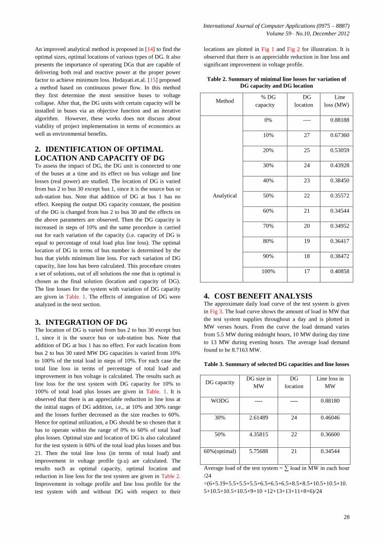
reduction in line loss for the test system are given in Table 2.

Improvement in voltage profile and line loss profile for the

test system with and without DG with respect to their

locations are plotted in Fig 1 and Fig 2 for illustration. It is

observed that there is an appreciable reduction in line loss and

significant improvement in voltage profile.

Table 2. Summary of minimal line losses for variation of

DG capacity and DG location

Method % DG

capacity

DG

location

Line

loss (MW)

Analytical

0% ---- 0.88188

10% 27 0.67360

20% 25 0.53059

30% 24 0.43928

40% 23 0.38450

50% 22 0.35572

60% 21 0.34544

70% 20 0.34952

80% 19 0.36417

90% 18 0.38472

100% 17 0.40858

4. COST BENEFIT ANALYSIS The approximate daily load curve of the test system is given

in Fig 3. The load curve shows the amount of load in MW that

the test system supplies throughout a day and is plotted in

MW verses hours. From the curve the load demand varies

from 5.5 MW during midnight hours, 10 MW during day time

to 13 MW during evening hours. The average load demand

found to be 8.7163 MW.

Table 3. Summary of selected DG capacities and line losses

DG capacity DG size in

MW

DG

location

Line loss in

MW

WODG ---- ---- 0.88180

30% 2.61489 24 0.46046

50% 4.35815 22 0.36600

60%(optimal) 5.75688 21 0.34544

Average load of the test system = ∑ load in MW in each hour

/24

=(6+5.19+5.5+5.5+5.5+6.5+6.5+6.5+8.5+8.5+10.5+10.5+10.

5+10.5+10.5+10.5+9+10 +12+13+13+11+8+6)/24



29

= 209.19/24 = 8.7163 MW

Size of DG = (8.7163+0.88180) * 60% = 5.75688 MW

The cost benefit analysis is carried out (without considering

environmental emissions and percentage of outage rate) for

the above selected DG capacities which are in Table 3 being

connected to their respective optimal locations. For base case

NPV analysis fixed cost of 1 MW DG plant is assumed at the

rate of 20, 00,000 $/MW. When DG is connected to the

system it is not run at 100% of rated capacity throughout the

day.

Fig 1: Impact of DG on voltage profile

Fig 2: Impact of DG on line loss profile

Fig 3: Daily load curve of the test system



30

The hourly loading pattern for 24 hours of a day on DG may

be scheduled as

22 hr to 24 hr and 00 hr to 04 hr (06 hrs) 30% of

rated capacity


rated capacity


rated capacity

Plant load factor (PLF) for a day = ∑ (Duration in

hours*percentage of rated capacity utilization)/24 =

(6*0.30+9*0.50+9*1)/24 = 63.75%

The pattern of loading may vary but it will consider the PLF

as 63.75% throughout all other calculations

DGkWh = PDG *24*PLF (1.1)

KWh loading of DG = rating of DG in KW * hours of the day

* PLF

= 5.75688(60%)*1000*24*0.637 = 88011 KWh or units/day

DG income has the two aspects, one is income from energy

generated and the other is from saving of energy due to line

loss reduction. The calculation procedure for those incomes as

follow:

DG a.inc = Celect*365(DGkWh + PLLR *PLF*24) (1.2)

Calculation procedure for optimal DG capacity:-

1. From above, 93278 units/day, calculated@ 0.088

$/unit which is the assumed fixed tariff at prevailing

rate of Distribution Company for domestic

consumers for a year.

= $ 0.088*88011*365 = $ 2826913

PLLR = Line loss without DG – Line loss with DG

= 0.88180 – 0.34544 = 0.5355 MW = 536.3 KW

2. Note that above KW saving is when the DG runs at

full load. Calculating the income in the same

manner as in (1) for a year

= $ 0.088*536.3*0.637*24*365 = $ 263350

Annual income from DG = $ 2826913 + 263350 = $

3090263

Above procedure is repeated for 30% and 50% DG capacities.

Fundamental to finance is the concept of “time value of

money,” where the assumption is that money is worth more in

your hand today then tomorrow. For example, money

available now can be invested to generate interest and revenue

which is a lost opportunity if one has to wait for money to

have at their disposal. The NPV, or net present worth (NPW),

of a time series of cash flows, both incoming (positive) and

outgoing (negative), is defined as the sum of the present

values (PVs) of the individual cash flows [16]. If all future

cash flows are incoming and the only outflow of cash is the

purchase price, the NPV is simply the PV of future cash flows

minus the purchase price [16]. NPV is a valuable tool in

discounted cash flow (DCF) analysis, is a standard method for

using the time value of money to appraise long-term projects

and is used for capital budgeting to measure the excess or

shortfall of cash flows in present value terms once financing

charges are met [16]. In this case, the financial benefit to

LDCs of increased DG uptake at strategic locations on the

distribution feeder is evaluated using NPV analysis. The NPV

of a sequence of cash flows takes as input the cash flows and

a discount rate or function and outputs a price; the converse

process in DCF analysis – taking a sequence of cash flows

and a price as input and inferring as output a discount rate

(e.g. “break even” discount rate which would yield the given

price as NPV) is called the yield, and is more commonly used

in finance, e.g. bond trading [17]. In this paper, a planning

period of twenty years was used to standardize the time

horizon so that a NPV analysis can be performed and the

financial benefits can be compared in present value terms.

Below are the expressions used in the NPV analysis.

CDGO&M= COMDG* DGkWh*365 (1.3)

CDGinstcost = PDG *CDGcapcost (1.4)

CDGenvcost = DGkWh *Cemiscost*365 (1.5)

Coutage = DG aninc *Routage (1.6)

Cdep = Rdep * CDGinstcost (1.7)

DGinbtax = DG a.inc - CDGO&M - Coutage – Cdep (1.8)

DGinaftax = DGinbtax - Rtax(DGinbtax) (1.9)

DGNPV = - CDGinstcost + (DGinaftax) (1.10)

For base case NPV analysis, it is assumed that the operation

and maintenance cost (O&M) and depreciation cost is 5% of

DG installation/investment cost. The equipment cost will be

written off to depreciation over a project life of 20 years. The

tax on income is assumed as 10% per annum and a 10% rate

of return per annum is expected as minimum but which may

be nullified by the hike of electricity tariff at the same rate. To

evaluate the impact of DG capacity on financial benefits, NPV

analysis has been performed on 30%, 50% and 60% DG

capacities. The financial analysis results for 30%, 50% and

60% DG capacities are given in Fig 4and Fig 5. From Fig 4

and Fig 5 it is observed that the year of cost recovery and

return on investment is varying with variation of DG capacity,

which represents a profitable operation.

5. SELECTION OF SUITABLE DG

TECHNOLOGY DG technologies can be classified as renewable and non-

renewable. Renewable include photovoltaic, wind,

geothermal, tidal, ocean. Nonrenewable include internal

combustion engine (gas or diesel or heavy oil), micro turbine,

fuel cells [18]. Almost all renewable DG technologies are non

dispatchable. For example wind turbine cannot be installed in



31

Fig 4: Illustration for return on investment with DG

Fig 5: Summary of cost benefit analysis with DG

Table 4. Economic summary of some DG technologies [17-

23]

Type of

Generation

Technology

Life Cycle

Emission

gCO2eq/ kWhe

Min ~ Max

Average Life

Cycle

Emission in

gCO2eq/ kWhe

F.F. Coal 800~1000 900

Oil Fired 700~800 750

Natural Gas Fired 360~575 467

PV 50~73 61.5

WT 8~30 19

Hydro 1~34 17.5

Bio-Mass 35~99 67

areas where there is no steady wind or in hurricane or cyclone

prone areas, same with the case of photovoltaic. So all DG

technologies have not yet proven to be cheap, clean and

reliable for field application. The economics and currently

available DG technologies are summarized in Table 4. In the

present study assuming the presumed benefits of DG

technologies, a selection process is carried out for the

implementation of project based on NPV analysis. Significant

emission cost of each DG technology has been calculated

based on [26] and presented in Table 4, where emission

includes pollutants like Co2, So2, Co, Nox. Based on Table 4,

NPV analysis has been carried out for various DG

technologies including environmental costs, and results are

illustrated in Fig 6 and Fig 7. From Fig 6 and Fig 7, it is

noticed that all DG Technologies doesn’t yield financial

benefits during the project period even though the emission

cost is negligible for technologies like WT and PV (this is due

to their higher initial investment cost as compared to other DG

technologies). Table 5. sets out typical life-cycle CO2

emissions of the major forms of electric power generation

technologies. Through the data in this table, it is found that

CO2 emissions from coal and biomass technologies are far

exceeded those of renewable energy technologies.



32

Fig 6: Summary of cost benefit analysis for various DG Technologies

Fig 7: Illustration for return on investment for various DG Technologies

Fig 8: Cumulative reduction of CO2 over project period in the presence of various DG Technologies



33

Fig 9: Cumulative production of CO2 over project period in the presence of various DG Technologies

Table 5. GHG (CO2) Emissions from Different Generation

Technologies

Type of

Generation

Technology

Life Cycle

Emission

gCO2eq/ kWhe

Min ~ Max

Average Life Cycle

Emission in

gCO2eq/ kWhe

F.F. Coal 800~1000 900

Oil Fired 700~800 750

Natural Gas

Fired 360~575 467

PV 50~73 61.5

WT 8~30 19

Hydro 1~34 17.5

Bio-Mass 35~99 67

Meanwhile it is observed that PV, WT, MH and FC

technologies are being regarded as an environmentally

friendly generation type. Cumulative reduction of CO2 over

the project period has been calculated based on [27, 28].

Cumulative reduction as well as production of CO2 over the

project period in the presence of different DG technologies is

illustrated in Fig 8 and Fig 9.

6. CONCLUSIONS In this paper, impact of DG on techno economic benefits has

been studied. Using 30-bus radial distribution test system and

DG capacities of 30%, 50% and 60% of total load plus losses,

the voltage profile and the real power loss has been analyzed

and significant improvement in voltage profile and reduction

in line loss is observed. For optimal utilization, a DG capacity

should be chosen that it has to operate with the capacity of

60% of total load plus losses. Profits have been estimated in

financial terms by performing NPV analysis for 20 years of

project period. It can be concluded that a distribution

company will definitely make profit only if a suitable size DG

plant is strategically placed in the distribution system. For the

implementation of project, a selection process is carried out

for suitable DG Technology and estimated the financial

benefits by considering emission cost and outage cost of DG.

It is recognized that selection of technology represents only a

technical option. The underlying economic reality and

financial benefits will determine whether this option is used or

not. In view of financial benefits not all DG technologies are

suitable for implementation of the project. It is observed that

greater use of renewable energy DG technologies can

significantly reduce the carbon intensity (CO2 emission) of

electricity generation in power sectors that are dominated by

fossil fuel power plants. Please note that, while the underlying

method and evaluation of DG in a radial distribution system

can be applied elsewhere. But, the financial results and

environmental benefits obtained in this study are purely

subjected to literature which cannot be generalized.

6. REFERENCES [1] Y H Song, G S Wang, A T Johns, PY Wang. Distribution

Network Reconfiguration for Loss Reduction using

Fuzzy Controlled Evolutionary Programming. IEE Proc.

Gene. Trans. Dist., 1997; 144: 345-350.

[2] YG Hejaz, MMA Salaam, AY Chicano. Adequacy

Assessment of Distributed Generation Systems using

Monte Carlo Simulation. IEEE Trans. On Power

Systems 2003; 18: 48–52.



34

[3] W EI-Khatan, MMA Salaam. Distributed generation

technologies, definitions and benefits. Electric Power

System Research 2004; 71:119-128.

[4] A Poullikkas. Implementation of distributed generation

technologies in isolated power systems. Renewable and

Sustainable energy 2007; 11:30-56.

[5] T Griffin, K Osmotic, D Secrets, A Low. Placement of

dispersed generation systems for reduced losses. In Proc.

IEEE 33rd Annul. Hawaii Int. Conf. Syst. Sciences

(HICSS) 2000; 1446 -1454.

[6] P Chiradeja. Benefit of distributed generation: a line loss

reduction analysis. T&D Conference and Exhibition:

Asia and Pacific 2005; 3:1401-1407.

[7] SS Pati, PK Modi. Loss minimization of distribution

system using distributed generation. Cogeneration and

Distributed Generation 2009; 24: 23-47.

[8] GP Harrison, AR Wallace. Optimal power flow

evaluation of distribution network capacity for the

connection of distributed generation. IEE Proc. Gen.

Trans. and Dist., 2005; 152: 115-122.

[9] A Silvestri, A Berizzi, S Buonanno. Distributed

generation planning using genetic algorithms. In

Proceedings of IEEE International Conference on

Electric Power Engineering, Power Tech., Budapest

1999; 99.

[10] W EI-Khatan, K Bhattacharya, Y Hegazy, MMA Salaam.

Optimal investment planning for distributed generation

in a competitive electricity market. IEEE Tans. On

Power Systems 2004; 19: 1674-1684.

[11] Jeo-Hao, Teng, Yi-Hwa, Liu, Chia-Yen, Chi-Fa Chen.

Value based distributed generation placements for

service quality improvements. Electrical Power and

Energy Systems 2007; 29: 268-274.

[12] W Rosehart, E Nowicki. Optimal placement of

distributed generation. In 14th Power Systems

Computation Conference 2002; 11: 1-5.

[13] BA Desouza, JMC De Albuquerque. Optimal placement

of distributed generators in network using evolutionary

programming. In proc. Of Trans. And Dist. Conference,

Latin America, IEEE/PES 2006: 1-6.

[14] DQ Hung, N Mithulanathan, RC Bansal. Analytical

expressions for DG allocation in primary distribution

networks. IEEE Trans. on Energy Conversion 2010; 25:

814-820.

[15] H Hedayati, SA Nabaviniaki, A Akbarimajd. A method

for placement of DG units in distribution networks.

IEEE Transactions on Power Delivery 2008; 23:1620-28.

[16] Net Present Analysis.

http://en.wikipedia.org/wiki/Net_present_value

[17] IEEE Application Guide for IEEE Std. 1547, IEEE

Standard for Interconnecting Distributed Resources with

Electric Power Systems (2008).

[18] N Jenkins, R Allan, P Crossley, D Kirschen, G Strbac.

Embedded generation. IEE Power and Energy. Series 31.

London; 2000.

[19] AGL. Comparison of large central and small

decentralized power generation in India. Golden, CO:

Antres Group Ltd. And NREL; 1997.

[20] EIA. Energy Information Administration. U.S

Department of energy. Annual Energy Outlook; 2002.

[21] J Gregory, S Silveira, A Derrick, P Cowley, C Allinson,

O Paish. Financing Renewable Energy Projects: A Guide

for Development workers. Intermediate Technology

Publications. London; 1997.

[22] Morris, Ellen. Analyses of Renewable Energy retrofit

Options to Existing Diesel Mini Grids. APEC.

Singapore; 1998.

[23] EM Petrie, HL Willis, M Takahashi. Distributed Power

Generation in Developing Countries. 2002. Available on

www.worldbank.org/html/fpd/em/distribution-abb.pdf.

[24] N Ravindranath, DO Hall. Biomass Energy and the

Environment: A Developing Country Perspective from

India. Oxford University Press, oxford; 1995.

[25] UN. Energy Issues and Options for Developing

Countries: Taylor and Francis. New York; 1989.

[26] K Qian, C Zhou, Y Yuan, X Shi, M Allan. Analysis of

the Environmental Benefits of Distributed Generation.

IEEE Power and Energy Society Meeting- Conversion

and Delivery of electrical energy in the 21st century

2008; 1-5.

[27] D Weisser. A guide to life-cycle greenhouse gas (GHG)

emissions from electric supply technologies Energy

2007; 32:19; 1543– 1559.

[28] IEA. CO2 Emissions from Fuel Combustion Highlights,

IEA Statistics, 2011 edition. Available on

www.iea.org/co2highlights.

analysis on techno-economic benefits of a strategically

Documents