analysis on products of fractals

TRANSACTIONS OF THEAMERICAN MATHEMATICAL SOCIETYVolume 357, Number 2, Pages 571–615S 0002-9947(04)03685-2Article electronically published on September 23, 2004

ANALYSIS ON PRODUCTS OF FRACTALS

ROBERT S. STRICHARTZ

Abstract. For a class of post–critically finite (p.c.f.) fractals, which includesthe Sierpinski gasket (SG), there is a satisfactory theory of analysis due toKigami, including energy, harmonic functions and Laplacians. In particular,the Laplacian coincides with the generator of a stochastic process constructedindependently by probabilistic methods. The probabilistic method is also avail-able for non–p.c.f. fractals such as the Sierpinski carpet. In this paper we showhow to extend Kigami’s construction to products of p.c.f. fractals. Since theproducts are not themselves p.c.f., this gives the first glimpse of what theanalytic theory could accomplish in the non–p.c.f. setting. There are someimportant differences that arise in this setting. It is no longer true that pointshave positive capacity, so functions of finite energy are not necessarily con-tinuous. Also the boundary of the fractal is no longer finite, so boundaryconditions need to be dealt with in a more involved manner. All in all, the

theory resembles PDE theory while in the p.c.f. case it is much closer to ODEtheory.

1. Introduction

Euclidean space may be constructed as a product of lines, and analysis on Eu-clidean space may be obtained by appropriately transporting corresponding con-cepts from the line. This will be our model for creating analysis on a product offractals. Because products of post–critically finite (p.c.f.) fractals are not p.c.f.,this enables us to construct an analytic theory on an entirely different kind of frac-tal. Indeed, the “differential equations” on p.c.f. fractals such as the Sierpinskigasket (SG) have much in common with ODE’s on the line or interval. We willsee that the analogous theory on products resembles PDE theory. Of course this isnot surprising. The point is that by exploiting the product structure we are ableto obtain significant results rather easily. We hope that this will serve as a modelfor what we can expect, and not expect, from analysis on a wider class of fractals.

The analytic theory on p.c.f. fractals was developed by Kigami [Ki1]–[Ki4] fol-lowing the work of several probabilists who constructed stochastic processes anal-ogous to Brownian motion, thus obtaining a Laplacian indirectly as the generatorof the process. See the book of Barlow [Ba] for an account of this development. Atpresent, both points of view have important consequences for the theory. Althoughwe emphasize the analytic development, we will need to use heat kernel estimates,

Received by the editors July 8, 2003.2000 Mathematics Subject Classification. Primary 31C45, 28A80.The author’s research was supported in part by the National Science Foundation, grant DMS–

0140194.

c©2004 American Mathematical Society

571

License or copyright restrictions may apply to redistribution; see https://www.ams.org/journal-terms-of-use

572 ROBERT S. STRICHARTZ

which are obtainable only via probability theory. The expository article [S3] ex-plains some of the goals of the theory in comparision with analysis on manifolds.We refer the reader to the book [Ki3] for complete details.

The four main concepts in analysis on p.c.f. fractals are: energy, harmonic func-tions, Laplacian, and resistance metric. The energy form E(u, v), the analog of∫ 1

0u′(x)v′(x)dx on the unit interval, is constructed as the limit of renormalized

graph energies on a sequence of graphs Γm approximating the fractal. This ap-proach is feasible because points have positive capacity, which implies that finiteenergy functions are continuous. This approach is not feasible in the product set-ting, for example in the case of the square. However, in Section 2 we are able togive several equivalent and natural definitions of E(u, v) in the product setting. Aharmonic function is defined to be an energy minimizer subject to boundary condi-tions. In the p.c.f. case the boundary is finite, so the space of harmonic functions isfinite dimensional, and it is best to think of harmonic functions as analogs of linearfunctions on the interval. In the product setting, the space of harmonic functionsis infinite dimensional. We give elementary properties of harmonic functions inSection 3, but postpone until Section 8 more precise results. For technical reasonswe introduce the more restricted class of pluriharmonic functions, that form a finitedimensional space, and may be computed precisely.

When we define a Laplacian ∆ in Section 4 we will show that harmonic functionscoincide with solutions of ∆h = 0. We use a weak form to define ∆, essentially

(1.1) −E(u, v) =∫

(∆u)vdµ

if v vanishes on the boundary. In the p.c.f. case it is possible to identify the L2

domain of ∆ with a natural Sobolev space, but this is not true in the productsetting. For example, there are many harmonic functions in the square that belongto the Sobolev space H1 but not H2. The key idea is that we need to have boundaryvalues in the appropriate boundary Sobolev spaces. In the p.c.f. we get this forfree because the boundary is so small. It is not until Section 7 that we are able topresent a full characterization of the appropriate Sobolev space of functions withLaplacians in L2. For functions in this Sobolev space we are able to prove some ofthe basic results known in the p.c.f. case, including existence of normal derivativeson the boundary and the Gauss–Green formula. We are also able to prove L2

boundedness of Riesz transforms and a Fubini–type characterization of the Sobolevnorm, results which have no analog in the p.c.f. setting. The Riesz transformsare clearly natural examples of the analog of Calderon–Zygmund operators in thissetting; at present there are no natural candidates for Calderon–Zygmund operatorson p.c.f. fractals, other than the Hilbert transform on the interval.

There is no analog of the resistance metric in the product setting; we do not seeany way to relate resistance networks to the structure of these fractals. Instead,we cobble together resistance metrics on each of the factors to define a metric onthe product, essentially mimicking the Pythagorean theorem in Euclidean space(more precisely a Finsler metric construction). In Section 6 we show easily thatheat kernel estimates extend from the factors to the product, using this metric.Heat kernel estimates have many pleasant consequences, and we use them in keyways in the rest of the paper.


ANALYSIS ON PRODUCTS OF FRACTALS 573

Because the boundary creates difficulties, we find it convenient to work in a“cover space” that has no boundary. In the p.c.f. setting, we construct the dou-ble cover by taking two copies of the fractal and identifying common boundarypoints. In [S6] we showed that in the case of SG the double cover fits into a generalframework of fractafolds, where every point has a neighborhood isomorphic to aneighborhood in the original fractal. While this is not necessarily the case for allp.c.f. fractals, it is still fairly easy to extend all constructions from the fractal toits double cover. In particular, the eigenfunctions of the Laplacian on the doublecover consist of just the odd extensions of Dirichlet eigenfunctions and the evenextensions of Neumann eigenfunctions on the fractal. In the product setting wesimply take the product of the double covers of the factors. For the case of thesquare this produces a quadruple cover by a 2–torus. In Section 5 we show how tocharacterize the domain of the energy form and the L2 domain of the Laplacian onthe cover space of a product fractal in terms of Sobolev spaces defined by eigen-function expansions. This enables us to prove a number of important properties.The issue of the corresponding properties on the product fractal is then reducedto an extension problem: which functions on the fractal can be extended to thecover to lie in the appropriate Sobolev space? For the domain of the energy formthis is trivial, since an even reflection suffices. For the L2 domain of the Laplacianwe show in Theorem 7.7 that extension is equivalent to the trace on the boundarybelonging to the appropriate Sobolev space.

Section 7 deals with traces and extensions relating Sobolev spaces on K and itsboundary. We are able to identify the correct trace space for normal derivatives,but the analog of Theorem 7.7 remains a conjecture. Section 8 deals with represen-tation formulas for harmonic functions, including an analog of the Poisson integral.In Section 9 we briefly discuss pointwise formulas for energy and Laplacian thatare valid under suitable regularity assumptions. In Section 10 we give characteri-zations of Sobolev spaces of small order, both in the p.c.f. and the product setting.These results seem rather generic, and should be valid in any context in whichthe appropriate heat kernel estimates are true. We conclude with Section 11 inwhich we discuss hypoellipticity properties. We show that harmonic functions areautomatically smooth, and we conjecture that u must be smooth on an open set if∆u = f and f is smooth on that open set.

The simplest example of a product fractal is the square, but it is not truly fractal,merely self–similar. All the results in this paper are already known for the square,although it may be difficult to find some of them in the literature. So perhaps thebasic example to consider is SG2 = SG×SG. This is a self–similar fractal generatedby an iterated function system (i.f.s.) of 9 mappings F ′i × F ′j for i, j = 1, 2, 3,where F ′i is the i.f.s. generating SG. Let q′1, q′2, q′3 denote the boundary pointsof SG. Then the boundary of SG2 is made up of six “faces”, three horizontal facesSG×q′i and three vertical faces q′i×SG. The 9 points (q′i, q′j) make up whatmight be called the distinguished boundary of SG2. Horizontal and vertical facesmeet at these points. The boundary forms a fractafold without boundary in thesense of [S6], but we will not use the spectral analysis of this fractafold here (justlike the identification of the boundary of the square with a circle does not play arole in analysis on the square). The 9 cells F ′i×F ′j(SG2) = F ′i (SG)×F ′j(SG) of level1 that make up SG2 intersect either at single points or on sets isomorphic to SG.In particular, SG2 is not finitely ramified: it remains connected after the removal



of finitely many points. (In fact, it should be possible to prove that to disconnectSG2 it is necessary to remove a set of the same dimension as SG.)

The construction of SG2 naturally embeds it in R4. Of course we need to em-phasize that, just as in the p.c.f. case, the analysis is based on the topology ofthe fractal, and not the geometry in any particular realization. In fact, SG withits resistance metric does not embed isometrically (or even quasi–isometrically) inany Euclidean space, and the same will be true for SG2 with the metric we use.Nevertheless, it would be desirable to have a geometric realization that allows usto “visualize” the fractal. The Hausdorff dimension of SG2 in its self–similar em-bedding in R4 is 2 log 3/ log 2 > 3, so this precludes a quasi–isometric embedding inR3. (Note added in proof : Maria Roginskaya has shown that SG2 does not embedtopologically in R3.)

A simpler product, [0, 1]×SG, is easy to visualize (a vertical stack of SG’s), butbecause of the mismatch of scaling factors we are not able to include this examplein many of our theorems. In fact the full strength of our theory only appliesto products with identical factors, and the scaling factors must be homogeneousthroughout the fractal. Of course, it can be argued that [0, 1]× SG is the naturalunderlying space for the space–time equations on SG, such as the heat and waveequation, that have been extensively studied [DSV], [CDS]. Indeed, the mismatchin scaling factors has already been identified as a cause for some of the unexpectedbehaviors of solutions of these equations. The product fractals discussed in thiswork allow a wide range of “differential operators” beside the Laplacian; futurework might reveal a full “fractal PDE” theory.

A finite element method numerical algorithm for SG2 has been worked out byBrian Bockelman, and is available at the website www.math.cornell.edu/∼stu28041/fem/index.htm.

We have structured the paper to add assumptions as we go along. In the earlysections we show that a reasonable theory exists on a wide class of products, butin order to obtain the more precise results of the later sections we have to narrowthe class of examples.

Some of our results depend on estimates for normal derivatives of the Dirichletheat kernel on the p.c.f. factors. At present, these estimates ((7.16), (8.3) and(8.11)) have not been established on any fractals (other than the interval). Webelieve that (8.11) is essentially trivial, but (7.16) and (8.3) are more challenging.Numerical evidence for (7.16) in the case of the Sierpinski gasket may be foundat the website www.math.cornell.edu/∼Bengal/ and in the paper [BSSY]. Heatkernel estimates in general require probabilistic methods, which are quite differentthan the methods used in this paper. We hope that by exhibiting some interestingconsequences of these estimates we will stimulate work on proving them.

Notation conventions. So as not to burden the reader with excessive notation, wework with prodcts of just two factors. The extension of the results to products withmore than two factors should be routine. We denote by a prime anything havingto do with the first factor, and by a double prime anything having to do with thesecond factor. Thus the product will be written K = K ′ ×K ′′, a variable point inK will be x = (x′, x′′). Similarly E ′ and ∆′ denote energy and Laplacian on K ′.This notation should be self–explanatory, and we hope it will help the reader easilygrasp the meaning of all equations. We also need to distinguish between spaces andtheir covers, and we do this by using a tilde for the cover. Thus K ′ and K ′′ denote



the double covers of K ′ and K ′′, and K = K ′ × K ′′ is the quadruple cover of K.We will not put tildes over variables, but by writing u′(x′) it will be clear that weare referring to a function on K ′.

Next we describe the basic assumptions on the factor K ′ (we make the sameassumptions about K ′′): K ′ is a p.c.f. self-similar set with boundary V ′0 , self–similar measure µ′ and self–similar regular energy E ′. For simplicty of notationwe assume that K ′ is embedded in some Euclidean space, and K ′ is the invariantset for a contractive linear iterated function system (i.f.s.) F ′ii=1,...,n′0

. Let q′idenote the fixed point of F ′i , and let V ′0 = qii=1,...,n′ for some n′ ≤ n′0. The p.c.f.condition is that K ′ is connected and

(1.2) F ′iK′ ∩ F ′jK ′ ⊆ F ′iV ′0 ∩ F ′jV ′0 for i 6= j.

We refer to the sets F ′iK′ as cells of level 1. In general we write w′ = (w′1, . . . , w

′m)

for a word of length |w′| = m, each w′j chosen from 1, . . . , n′0, and F ′w′ = F ′w′1

· · · F ′w′m . Then the sets F ′w′K′ are called cells of level m. Distinct cells of a given

level can intersect only at isolated points. The self–similar probability measure µ′

is determined by the choice of probability weights µ′ii=1,...,n′0via the identity

(1.3) µ′ =n′0∑i=1

µ′iµ′ (F ′i )

−1,

or equivalently

(1.4)∫K′fdµ′ =

n′0∑i=1

µ′i

∫f F ′idµ′.

To define the self–similar energy we consider K ′ as the limit of graphs Γ′m withvertices V ′m and edge relation x′ ∼m y′ defined inductively as follows: Γ′0 is thecomplete graph on V ′0 , and V ′m =

⋃n′0i=1 F

′iV′m−1 and x′ ∼m y′ if and only if x′

and y′ belong to the same cell F ′w′K′ of level m. We choose positive conductances

c′ij = c′ji for i 6= j, i, j = 1, . . . , n′. In other words c′ are defined on the edgesof the graph Γ′0. We may think of the reciprocals as resistances in an electricalnetwork with vertices V ′0 . We choose also resistance renormalization factors r′ifor i = 1, . . . , n′0 satisfying 0 < r′i < 1. Then we create a self–similar electricalnetwork on Γ′m by defining c′x′y′ = (r′w′)

−1c′ij if x′ = F ′w′q′i and y′ = F ′w′q

′j , where

r′w′ = r′w′1· · · r′w′m . Note that the condition r′i < 1 means that the resistances of the

edges tend to zero as m → ∞. The energy E ′m(u′, v′) for u′, v′ functions on V ′m isdefined by

(1.5) E ′m(u′, v′) =∑

x′∼my′cx′y′(u′(x′)− u′(y′))(v′(x′)− v′(y′)).

Note that we also have

(1.6) E ′m(u′, v′) =∑|w′|=m

(r′w)−1E ′0(u′ F ′w, v′ F ′w).

This alone is not enough to enable us to pass to the limit as m→ ∞. We needone more very restrictive compatibility condition:

(1.7) E ′1(u′, u′) = E ′0(u′, u′),



where u′ is chosen among all extensions of u′ to V ′1 so as to minimize E ′1 (this is calledthe harmonic extension). This places rather complicated nonlinear constraints onthe initial conductances and resistance renormalization factors. Questions aboutexistence and uniqueness of such energies are still not completely resolved, but itsuffices for our purposes to note that there are many explicit examples known,including the unit interval I (both r′i = 1/2) and SG (all c′ij = 1 and all r′i = 3/5).

It follows easily from (1.7) that E ′m(u′, u′) is a monotone increasing function forany u′ defined on K ′, hence

(1.8) E ′(u′, u′) = limm→∞

E ′m(u′, u′)

is well defined as an extended real number, and we define dom E ′ to be the functionsfor which the limit is finite. The basic facts are that dom E ′ is a dense subspace ofC(K ′), and modulo constants it forms a Hilbert space with norm E ′(u′, u′)1/2. Foru′, v′ ∈ dom E ′,

(1.9) E ′(u′, v′) = limm→∞

E ′m(u′, v′)

is well defined and gives the inner product. There is an n′-dimensional space H′0 ofharmonic functions obtained by assigning values in V ′0 , taking the minimum energyextension at each level, and extending from V ′∗ =

⋃∞m=0 V

′m to K ′ by continuity. For

harmonic functions, E ′m(u′, u′) is independent of m (in fact E ′m(u′, v′) is independentof m if just u′ is harmonic). The self–similarity of the energy E ′ may be expressedas

(1.10) E ′(u′, v′) =n′0∑i=1

(r′i)−1E ′(u′ F ′i , v′ F ′i ),

or more generally

(1.11) E ′(u′, v′) =∑|w′|=m

(r′w′)−1E ′(u′ F ′w′ , u′ F ′w′).

Given the energy E ′, we define a natural metric, called the effective resistancemetric on K ′, by

(1.12) d(x′, y′) = (minE(u, u) : u(x′) = 0 and u(y′) = 1)−1.

An important observation is that this metric has nothing to do with the Euclideanmetric of the ambient space where K ′ is embedded. The construction of E ′ infact only uses the topology of K ′, and it can be shown that the effective resistancemetric yields the same topology. In most examples, the fractal K ′ with the effectiveresistance metric will not embed isometrically (or even quasi–isometrically) in anyEuclidean space. The effective resistance metric is not exactly self–similar, but isapproximately self–similar: each cell F ′w′K

′ has diameter on the order of r′w′ .Given the energy E ′ and measure µ′, we define a Laplacian ∆′ with domain

dom ∆′ as follows: u′ ∈ dom ∆′ with ∆′u′ = f ′ for u′ ∈ dom E ′ and f ′ ∈ C(K ′)provided

(1.13) −E ′(u′, v′) =∫K′f ′v′dµ′ for all v′ ∈ dom0E ,



where dom0E ′ denotes the subspace of dom E ′ of functions vanishing on the bound-ary V ′0 . There is also an equivalent pointwise formula

(1.14) ∆′u′ = limm→∞

∆′mu′

for the graph Laplacian

(1.15) ∆′mu′(x′) =

( ∫ψ

(m)x′ dµ

′)−1 ∑

y′∼mx′c′x′y′(u

′(y′)− u′(x′)),

where ψ(m)x′ is the piecewise harmonic spline of level m equal to 1 at x′ and 0 at

all other vertices in V ′m. The limit (1.14) must be uniform (note that ∆′mu′ is not

defined on V ′0 , however) in a suitable sense. (On SG (1.15) takes the simple form

(1.16) ∆′mu′(x′) =

(32

)5m

∑y′∼mx′

(u′(y′)− u′(x′))

for x′ ∈ V ′m \ V ′0 , and there are exactly four terms in the sum (1.16).) We alsodefine domL2∆′ by requiring (1.13) to hold for some f ′ ∈ L2. The equivalentpointwise formula would require the limit (1.14) to hold in a suitable L2 sense.(This equivalence is not explictly stated in the literature, but should be fairlystraightforward to derive.) The Laplacian satisfies the scaling identity

(1.17) ∆′(u′ F ′w′) = rwµw(∆u′) F ′w′ .Another important concept is the normal derivative at boundary points. The

definition only depends on E ′:

(1.18) ∂nu′(q′i) = lim

m→∞(r′i)−m

∑y′∼mq′i

(u′(q′i)− u′(y′))

if the limit exists. But the theorem guaranteeing existence requires that u′ ∈dom ∆′ (or domLq∆′). (Note that this will hold for any choice of weights µ′idefining µ, even though these weights do not enter into (1.18).) We can then statetwo forms of the Gauss–Green formula:

(1.19) −E ′(u′, v′) =∫K′

(∆′u′)v′dµ−∑V ′0

(∂nu′)v′

for u′ ∈ domL2∆′ and v′ ∈ dom E ′, and

(1.20)∫K′

((∆′u′)v′ − u′∆′v′)dµ′ =∑V ′0

((∂nu′)v′ − u′∂nv′)

for u′, v′ ∈ domL2∆′. These formulas also localize to any cell.

2. Energy

Suppose we are given energy forms E ′ on K ′ and E ′′ on K ′′, and probabilitymeasures µ′ on K ′ and µ′′ on K ′′. We can then construct an energy form E on Kwith domain dom E that we can represent schematically as E ′ × µ′′ + µ′ × E ′′ asfollows.

Definition 2.1. For u ∈ L2(K,µ′ × µ′′) let

(2.1) E(u, u) =∫K′′E ′(u(·, x′′), u(·, x′′))dµ′′(x′′) +

∫K′E ′′(u(x′, ·), u(x′, ·))dµ′(x′).



We say u ∈ dom E if E(u, u) <∞. For u and v in dom E we let

(2.2) E(u, v) =∫K′′E ′(u(·, x′′), v(·, x′′))dµ′′(x′′) +

∫K′E ′′(u(x′, ·), v(x′, ·))dµ′(x′).

If C = FwK is any cell, then we define similarly EC(u, u), the energy restricted toC. We do the same for any simple subset of K, defined to be a finite union of cells.

We assume that E ′, µ′, E ′′, µ′′ are self–similar with weights r′i, µ′i and r′′j , µ′′j for

mappings F ′i and F ′′j . It is only in very special cases that E is self–similar for themappings F ′i ⊗ F ′′j .

Lemma 2.2. Suppose there is a positive constant b such that r′iµ′i = b−1 and

r′′j µ′′j = b−1 for all i and j. Then E is self–similar with weights br′ir

′′j for the

mapping F ′i ⊗ F ′′j , namely

(2.3) E(u, v) =n′∑i=1

n′′∑j=1

(br′ir′′j )−1E(u (F ′i ⊗ F ′′j ), v (F ′i ⊗ F ′′j )).

Proof. The self–similarity properties of E ′ and µ′′ imply∫K′′E ′(u(x′, x′′), v(x′, x′′))dµ′′(x′′)

=n′∑i=1

n′′∑j=1

(µ′′j /r′i)E ′(u(F ′ix

′, F ′′j x′′), u(F ′ix

′, F ′′j x′′))dµ′′(x′′).

We obtain a similar expression with a factor of (µ′i/r′′j ) for the second term in (2.2).

But our assumptions imply r′i/µ′′j = r′′j /µ

′i = br′ir

′′j .

For the case of the square, r′i = µ′i = 1/2 and b = 4, so br′ir′′j = 1 and (2.3) is a

special case of the conformal invariance of energy. For the case of SG2, r′i = 3/5 andµ′i = 1/3 so b = 5 and br′ir

′′j = 9/5. In the symmetric case K ′ = K ′′, if we are given

a self–similar energy E ′ = E ′′ with weights r′i, we can always choose a self–similarmeasure µ′ = µ′′ to satisfy the hypotheses of Lemma 2.2, namely take µ′i = (br′i)

−1

for b =∑r−1i . Note, however, that this differs from what is usually considered the

natural choice (µ′i = (r′i)α where

∑(r′i)

α = 1), unless all the ri weights are equal.It is easy to construct functions in dom E by taking tensor products of dom E ′ and

dom E ′′. In the next definition we single out a special case of such a constructionthat will be very useful.

Definition 2.3. A function on K is called pluriharmonic if it satisfies both∆′x′u(x′, x′′) = 0 and ∆′′x′′u(x′, x′′) = 0. The space of pluriharmonic functions,denoted PH, coincides with H′0 ⊗H′′0 , with dimension n′n′′, and natural basis

(2.4) hij(x′, x′′) = h′i(x′)h′′j (x′′).

A function u ∈ PH is uniquely determined by its values on the distinguished bound-ary V ′0 × V ′′0 by

(2.5) u =n′∑i=1

n′′∑j=1

u(q′i, q′′j )hij .

A function is called piecewise pluriharmonic of level m (PPHm) if u is continuousand u(F ′w′x

′, F ′′w′′x′′) ∈ PH for all words w′ and w′′ of length m. A function in



b0 b0 b0

b0

b0

b1b1 b1

b1

b1

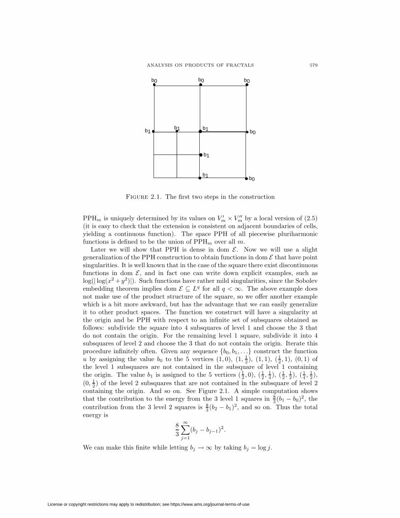
Figure 2.1. The first two steps in the construction

PPHm is uniquely determined by its values on V ′m × V ′′m by a local version of (2.5)(it is easy to check that the extension is consistent on adjacent boundaries of cells,yielding a continuous function). The space PPH of all piecewise pluriharmonicfunctions is defined to be the union of PPHm over all m.

Later we will show that PPH is dense in dom E . Now we will use a slightgeneralization of the PPH construction to obtain functions in dom E that have pointsingularities. It is well known that in the case of the square there exist discontinuousfunctions in dom E , and in fact one can write down explicit examples, such aslog(| log(x2 +y2)|). Such functions have rather mild singularities, since the Sobolevembedding theorem implies dom E ⊆ Lq for all q < ∞. The above example doesnot make use of the product structure of the square, so we offer another examplewhich is a bit more awkward, but has the advantage that we can easily generalizeit to other product spaces. The function we construct will have a singularity atthe origin and be PPH with respect to an infinite set of subsquares obtained asfollows: subdivide the square into 4 subsquares of level 1 and choose the 3 thatdo not contain the origin. For the remaining level 1 square, subdivide it into 4subsquares of level 2 and choose the 3 that do not contain the origin. Iterate thisprocedure infinitely often. Given any sequence b0, b1, . . . construct the functionu by assigning the value b0 to the 5 vertices (1, 0), (1, 1

2 ), (1, 1), (12 , 1), (0, 1) of

the level 1 subsquares are not contained in the subsquare of level 1 containingthe origin. The value b1 is assigned to the 5 vertices ( 1

2 , 0), (12 ,

14 ), (1

2 ,12 ), (1

4 ,12 ),

(0, 12 ) of the level 2 subsquares that are not contained in the subsquare of level 2

containing the origin. And so on. See Figure 2.1. A simple computation showsthat the contribution to the energy from the 3 level 1 squares in 8

3 (b1 − b0)2, thecontribution from the 3 level 2 squares is 8

3 (b2 − b1)2, and so on. Thus the totalenergy is

83

∞∑j=1

(bj − bj−1)2.

We can make this finite while letting bj →∞ by taking bj = log j.



Theorem 2.4. Suppose the hypotheses of Lemma 2.2 hold with br′jr′′k > 1 for some

(j, k). Then there exists a function u ∈ dom E with pole at (qj , qk) that does notbelong to Lq for

(2.6) q > 2 +2 log b

log(br′jr′′k )

.

Proof. Given q satisfying (2.6) choose the sequence b0, b1, . . . to be

(2.7) bm = (b2r′jr′′k )m/q.

Assign values to u as follows: u(q′`, q′′n) = b0 provided (`, n) 6= (j, k); u(F ′jq

′`, F

′′k q′′n) =

b1 provided (`, n) 6= (j, k); and u = b0 at all other points of V ′1 ×V ′′1 except (q′j , q′′k ).

Then extend u to be PPH on all level 1 cells except F ′jK′ × F ′′kK

′′. Next weassign values for u at each of the vertices of order 2 lying in F ′jK

′ × F ′′kK ′′ except(qj , qk), namely u((F ′j)

2q′`, (F′′k )2q′′n) = b2 provided (`, n) 6= (j, k), and u = b1 at

the remaining vertices. We extend u to be PPH on all level 2 cells contained inF ′jK

′ × F ′′kK ′′ except (F ′j)2K ′ × (F ′′k )2K ′′. And so on.

The values of u on the V ′1×V ′′1 vertices of the level 1 cells (except F ′jK′×F ′′kK ′′)

are either b0 or b1, so the contribution to the energy from these cells is exactlyc (b1−b0)2

(br′jr′′k ) for a positive constant c whose exact value is not important. But then the

contributions to the energy from the level 2 cells is exactly c (b2−b1)2

(br′jr′′k )2 , and so on, so

(2.8) E(u, u) = c

∞∑m=1

(bm − bm−1)2

(br′jr′′k )m

.

We note that the choice (2.7) allows us to bound E(u, u) by a convergent geometricsum exactly when (2.6) holds. On the other hand, similar estimates allow us toapproximate ‖u‖qq from above and below by multiples of

(2.9)∞∑m=1

bqm(µ′jµ′′k)m =

∞∑m=1

bqm(b2r′jr

′′k )m

.

The choice (2.7) makes each term in (2.9) equal to 1, so u /∈ Lq.

We will see later that for many examples (2.6) is sharp, since dom E ⊆ Lq for qequal to the right side of (2.6).

Because dom E contains discontinuous functions, we have to exercise some cau-tion in working with pointwise values of functions in dom E . However, it is clearfrom the definition that for u ∈ dom E we must have u(·, x′′) ∈ dom E ′ and hencecontinuous for almost every choice of x′′, and similarly u(x′, ·) is continuous foralmost every x′. So there is no harm in making this assumption (rather than justu ∈ L2) from the beginning, which we will call minimal regularity.

Theorem 2.5. A function u with minimal regularity belongs to dom E if and onlyif

(2.10) supm

∫K′′E ′m(u(·, x′′), u(·, x′′))dµ′′(x′′)

and

(2.11) supm

∫K′E ′′m(u(x′, ·), u(x′, ·))dµ′(x′)



are both finite. If u and v are in dom E, then

E(u, v) = limm→∞

( ∫K′′E ′m(u(·, x′′), v(·, x′′))dµ′′(x′′)

+∫K′E ′′m(u(x′, ·), v(x′, ·))dµ′(x′)

).

(2.12)

Proof. The minimal regularity implies E ′m(u(·, x′′), u(·, x′)) is well defined for almostevery x′′, and E ′′m(u(x′, ·), u(x′, ·)) is well defined for almost every x′. Since E ′m andE ′′m are monotone increasing in m, if u ∈ dom E , then

E ′m(u(·, x′′), u(·, x′′)) ≤ E ′(u(·, x′′), u(·, x′′))so∫

K′′E ′m(u(·, x′′), u(·, x′′))dµ′′(x′′) ≤

∫K′′E ′(u(·, x′′), u(·, x′′))dµ′′(x′′) ≤ E(u, u).

This shows (2.10) is finite, and similarly (2.11) is finite. Conversely, if (2.10) and(2.11) are finite, then the monotone convergence theorem shows that u ∈ dom E ,and (2.12) holds for u = v. The general case of (2.12) follows by polarization.

Remark. Under the assumptions of Lemma 2.2 we can interpret this characteriza-tion in a way that is analogous to the construction of energy in the p.c.f. case.Let

E0(u, u) =∫K′′E ′0(u(·, x′′), u(·, x′′))dµ′′(x′′) +

∫K′E ′′0 (u(x′, ·), u(x′, ·))dµ′(x′)

(the sum of the m = 0 terms in (2.10) and (2.11)). We interpret this as a crudeapproximation to the energy at level 0. Note that it depends only on the boundaryvalues of u. We then create a more refined level m approximate energy by taking

Em(u, u) =∑|w′|=m

∑|w′′|=m

(bmr′w′r′′w′′)−1E0(u (F ′w′ × F ′′w′′), u (F ′w′ × F ′′w′′)),

the sum over all cells of level m of the appropriately renormalized crude energyof the restriction of u to that cell. The point is that this is just the sum of theindividual terms in (2.10) and (2.11); the assumptions of Lemma 2.2 guaranteethe same renormalization factor for both terms. So (2.12) (for u = v) says thatE(u, u) = lim

m→∞Em(u, u), and the limit is monotone increasing.

However, there are some differences compared to the p.c.f. case. We cannotassert that E0(u, u) is equal to E(u, u) if u is harmonic, so E0(u, u) is not the“natural choice” for crude energy. We will return to this issue in Section 8. Wedo note that E0(u, u) gives the correct energy for pluriharmonic functions, so thelimit in (2.12) is attained for finite m if u is PPH.

Another difference is that the renormalization factors in (2.3) do not uniquely(up to a constant multiple) determine the energy, as is often the case for p.c.f.fractals [M], [P], [Sa], [SST]. Indeed, we could modify (2.1) by multiplying eachintegral by an independent positive constant, and (2.3) would still hold. All theseenergies are different, although they are equivalent (each is bounded by a multipleof any other). We must choose E0(u, u) carefully in order to obtain the exact valueof the energy in the limit.

The next characterization of energy involves “multiple Fourier series”; specifi-cally, expansions in products of Neumann eigenfunctions for the Laplacians ∆′ and



∆′′. Let u′j and u′′k denote orthonormal bases for L2(K ′, µ′) and L2(K ′′, µ′′),respectively, of such eigenfunctions, so

(2.13)

−∆′u′j = λ′ju

′j, ∂

′nu′j(q′`) = 0,

−∆′′u′′k = λ′′ku′′k, ∂

′′nu′′k(q′′n) = 0,

with

(2.14)

0 = λ′0 < λ′1 ≤ λ′2 ≤ · · · ,0 = λ′′0 < λ′′1 ≤ λ′′2 ≤ · · · .

Then clearly ujk(x′, x′′) = u′j(x′)u′′k(x′′) gives an orthonormal basis for L2(K). We

will write

(2.15) u =∞∑j=0

∞∑k=0

ajk(u)ujk

with

(2.16) ajk(u) =∫K

u · ujkdµ

for the expansion of u ∈ L2(K) in this basis, so

(2.17)∫K

uvdµ =∞∑j=0

∞∑k=0

ajk(u)ajk(v).

Theorem 2.6. u ∈ dom E if and only if

(2.18)∞∑j=0

∞∑k=0

(λ′j + λ′′k)ajk(u)2

is finite, in which case (2.18) equals E(u, u). More generally

(2.19)∞∑j=0

∞∑k=0

(λ′j + λ′′k)ajk(u)ajk(v) = E(u, v)

for u and v in dom E.

Proof. We use the analogous characterization of dom E ′ and dom E ′′; specifically

u′ ∈ dom E ′ if and only if∞∑j=0

λ′ja′j(u′)2 is finite, in which case it equals E ′(u′, u′),

for a′j(u′) =

∫K′u′u′jdµ

′, and similarly for dom E ′′. This result is well known butperhaps not stated explicitly in the literature. A proof for the special case SG isgiven in [S5], Theorem 3.7 (d), and the same proof works in general. Note that it isimportant to use Neumann eigenfunctions, as the analogous statement is not validfor Dirichlet eigenfunctions.

The proof is now easy. Fix x′′ and note that

E ′(u(·, x′′), u(·, x′′)) =∞∑j=0

λ′j

( ∞∑k=0

ajk(u)u′′k(x′′))2



because∞∑k=0

ajk(u)u′′k(x′′) = a′j(u(·, x′′)). Integrate with respect to x′′ and use the

orthonormality of u′′k to obtain∫K′′E ′(u(·, x′′), u(·, x′′))dµ′′(x′′) =

∞∑j=0

λ′j

( ∞∑k=0

ajk(u)2).

Do a similar argument in the reverse order and add the two to obtain the equalityof (2.18) and E(u, u). The rest of the argument is routine.

Corollary 2.7. (a) For u ∈ dom E, E(u, u) = 0 if and only if u is constant. (b)The space dom E modulo constants forms a Hilbert space with inner product E(u, v).(c) dom E is dense in L2. (d) dom E/constants ⊆ L2 is compact. (e) PPH is densein dom E.

Proof. Note that u′0, u′′0 and u00 are all constant, and λ′j + λ′′k = 0 if and onlyif j = k = 0. (a), (b) and (c) follow easily. (d) follows because the sequenceλ′j + λ′′k arranged in increasing order tends to infinity. To prove (e) note thatfinite sums of the form (2.15) are dense in dom E , so it suffices to show that eachujk may be approximated in energy by PPH functions. But u′j and u′′k may eachbe approximated, both in L2 and energy, by piecewise harmonic functions ϕ′jε andϕ′′kε, so ϕ′jε(x

′)ϕ′′kε(x′′) approximates ujk in energy.

The next result says that E satisfies the Markov property.

Theorem 2.8. Let u ∈ dom E and let v(x) = max(a,min(u(x), b)) for any fixedconstants a, b with a < b. Then v ∈ dom E and E(v, v) ≤ E(u, u).

Proof. This result is known for E ′ and E ′′, and it transfers to E directly from(2.1).

For the next energy formula, using the method of average values originally dueto Kusuoka and Zhou [KZ], we restrict attention to K = SG2. No doubt there areanalogous results in the general case, but the preliminary work in the p.c.f. casehas not yet been done. For a function u′ defined on SG, we define the averages oncells F ′w′(SG) by

Aw′(u′) = 3m∫F ′w′(SG)

u′(x′)dµ′(x′)

=∫

SG

u′(F ′w′x′)dµ′(x′)

(2.20)

for |w′| = m. Two cells of level m are adjacent if they have a point in common,and we write w′ ∼m w′. Note that a nonboundary cell always has exactly threeneighbors. In [S4] we showed that

(2.21) E ′(u′, u′) = limm→∞

32

(53

)m ∑w′∼mw′

(Aw′(u′)−Aw′(u′))2,

so dom E ′ is characterized by the finiteness of the limit on the right of (2.21). Infact we showed more precisely that

(2.22) E ′m(u′, u′) =32

((35

)m−(3

5

)2m)−1 ∑w′∼mw′

(Aw′(u′)−Aw′(u′))2



if u′ is harmonic, so that by adjusting the constant in (2.21) we have a monotonelimit.

Similarly, for u defined on SG2 and a cell Fw(SG2) of level m, so w = (w′, w′′)with |w′| = |w′′| = m, we define the average

Aw(u) = 9m∫F ′w′ (SG)

∫F ′′w′′ (SG)

u(x′, x′′)dµ′(x′)dµ′′(x′′)

=∫

SG2u(Fwx)dµ(x).

(2.23)

The adjacency relation w ∼m w will mean that either w′ ∼m w′ and w′′ = w′′, orw′ = w′ and w′′ ∼m w′′. In other words, the two cells must intersect along a setequivalent to SG, not just at an isolated point.

Theorem 2.9. For u and v in dom E on SG2,

(2.24) E(u, v) = limm→∞

32

(59

)m ∑w∼mw

(Aw(u)−Aw(u))(Aw(v) −Aw(v)).

Proof. Suppose w′ ∼m w′ and w′′ = w′′. Then

Aw(u)−Aw(u) = 3m∫F ′′w′′ (SG)

(Aw′(u(·, x′′))−Aw′(u(·, x′′)))dµ′′(x′′).

By Cauchy–Schwartz∑|w′′|=m

∑w′∼mw′

|Aw(u)−Aw(u)|2

≤ 3m∫

SG

∑w′∼mw′

|Aw′(u(·, x′′))−Aw′(u(·, x′′))|2dµ(x′′)

hence

limm→∞

(32

)(59

)m ∑|w′′|=m

∑w′∼mw′

|Aw(u)−Aw(u)|2

≤∫

SG

E ′(u(·, x′′), u(·, x′′))dµ′′(x′′)

by (2.21) and the monotone convergence theorem. By a similar argument in thecase w′ = w′ and w′′ ∼m w′′, and adding, we see that

(2.25) limm→∞

32

(59

)m ∑w∼mw

(Aw(u)−Aw(u))2 ≤ E(u, u).

If u is also continuous, it is easy to see that we have equality in (2.25). Inparticular, if u is represented by a finite sum in (2.15). Such functions are dense indom E , and we may use (2.25) to control the remainder, to obtain equality for allu ∈ dom E . By polarization we then obtain (2.24).

It seems likely that there is a full equivalence, so that the finiteness of the limitin (2.25) for u of minimal regularity would imply u ∈ dom E . However, the proofwould have to be quite technical, so we will not attempt it here.



3. Harmonic functions

In this section we require the assumptions of Lemma 2.2. We want to define har-monic functions as energy minimizers, subject to boundary conditions. We observethat functions in dom E have well–defined boundary values in L2 by Theorem 2.5.The converse is of course not true. In Section 7 we will be able to give a rathercomplete description of the “trace space” of dom E , but we will side–step the issuein this section by simply assuming that we are given a function ϕ in L2(∂K) thatis the boundary value of a function in dom E .

Theorem 3.1. Let ϕ ∈ L2(∂K) be the boundary values of some u ∈ dom E. Thenthere is a unique function h ∈ dom E which achieves the minimum value of E(v, v)for all v ∈ dom E with v

∣∣∂K

= ϕ. Moreover h depends linearly on ϕ.

Proof. Let Bϕ be the subset of dom E given by boundary condition v|∂K = ϕ. Bϕis an affine subspace transverse to the constants, so E(u − v, u − v)1/2 is a metricon Bϕ, and Bϕ is closed and hence complete in this metric (using Theorem 2.5 andCorollary 2.7 (b)). Let m denote the infinum of E(u, u) over Bϕ. The key estimateis

(3.1)12

(E(u, u) + E(v, v)) − E(u− v

2,u− v

2

)= E

(u+ v

2,u+ v

2

)≥ m

for u and v in Bϕ, since Bϕ is convex. If uk is a minimizing sequence in Bϕ, then(3.1) implies

E(uj − uk, uj − uk) ≤ 2(E(uj , uj) + E(uk, uk))− 4m,

which shows that uk is a Cauchy sequence. By completeness, uk converges inthe energy metric. Call the limit h. Clearly h is a minimizer. The uniqueness alsofollows by applying (3.1) to two minimizers h1 and h2. We obtain

E(h1 − h2, h1 − h2) = 0

so h1 = h2 because they are equal on the boundary.

Definition 3.2. A function h in dom E is said to be a harmonic function of finiteenergy if h minimizes energy among functions with the same boundary values. IfΩ is any open set in K and h is a function defined on Ω, we say h is harmonic inΩ if for any simple subset C =

⋃FwK contained in the interior of Ω, h minimizes

EC(u, u) over all functions u with the same values on ∂C.

In order for the definition to be consistent we need to verify the following:

Lemma 3.3. If h is harmonic with finite energy, then h Fw is harmonic withfinite energy for any word w.

Proof. By (2.3) iterated we may write the energy of h as a sum of contributionsfrom all cells of a fixed level m,

(3.2) E(h, h) =∑|w|=m

(bmrw)−1E(h Fw, h Fw).

Suppose for one choice w of w the function hFw did not achieve the minimum forits boundary values, so E(v, v) < E(h Fw, h Fw) while v|∂K = h Fw

∣∣∂K

. Then



we could construct a function h as follows:

h(x) =

h(x) if x /∈ FwK,v(F−1

w x) if x ∈ FwK.

The boundary conditions imply that h = h on the closure of the complement ofFwK, so when we compute E(h, h) using (3.2) all the terms corresponding to w 6= w

are the same, while the one corresponding to w = w is smaller. But h|∂K = h|∂K ,contradicting the minimality of h.

Harmonic functions of finite energy satisfy a form of the maximum principle.

Theorem 3.4. Let h be a harmonic function of finite energy with boundary valuesϕ. Suppose ϕ is bounded from above (or below). Then h is bounded from above (orbelow) by the same bounds.

Proof. Suppose ϕ ≤M . Let v(x) = min(u(x),M). Then v has the same boundaryvalues as h. But E(v, v) ≤ E(h, h) by Theorem 2.8, so by the uniqueness of theminimizer in Theorem 3.1 we must have v = h, hence h ≤M . The same argumentworks for lower bounds.

The same result localizes to any simple subset.It follows by the Hahn–Banach theorem that we have a “harmonic measure”

representation of h in terms of its boundary values: for each x in the interior of Kthere exists a probability measure νx on ∂K such that

(3.3) h(x) =∫∂K

ϕ(y)dνx(y).

In Section 8 we will give a more precise description of the harmonic measure as a“Poisson integral”.

4. The Laplacian

Given the energy constructed in Section 2 and a reasonable measure ν on K, wemay define a Laplacian ∆ν via the weak formulation

(4.1) −E(u, v) =∫K

(∆νu)vdν

for all v ∈ dom0E , the subspace of dom E of functions vanishing on the boundary.For simplicity we will restrict attention to the case ν = µ.

Definition 4.1. For u ∈ dom E and f ∈ C(K), we say u ∈ dom ∆ and ∆u = fprovided

(4.2) −E(u, v) =∫fvdµ for all v ∈ dom0E .

If f ∈ Lq(K) for some q ≥ 2 and (4.2) holds, we say u ∈ domLq∆. Note thatthe right side of (4.2) is well defined since dom E ⊆ L2. (Later we will be able toreduce the lower bound on q, but q = 2 is the case we will consider most often.)Note that it suffices to verify (4.2) for all v ∈ PPH vanishing on the boundary, byCorollary 2.7 (c). If Ω is an open set in the interior of K, we will say ∆u = f on Ωif (4.2) holds for all v ∈ dom E with support in Ω. Here we may allow f ∈ C(Ω) orf ∈ Lqloc(Ω).

It is easy to see that dom0E is dense in L2, so f is uniquely determined by (4.2).



Next we give a variational formulation of ∆u = f .

Theorem 4.2. Let u ∈ dom E with boundary values ϕ, and let Bϕ denote theaffine subspace of dom E of all functions with boundary values ϕ. Let f ∈ C(K)(respectively f ∈ Lq(K) for some q ≥ 2). Then u ∈ dom ∆ (respectively u ∈domLq∆) and ∆u = f if and only if u minimizes

(4.3)12E(v, v) +

∫fvdµ

over all v ∈ Bϕ. Moreover, the minimum is unique.

Proof. Note that (4.3) is a strictly convex functional on Bϕ, so every critical pointis a minimum, and there is at most one minimum. So it suffices to show that criticalpoints of (4.3) are the same as solutions of (4.2). Also note that if v ∈ dom0E , then(u+ tv) ∈ Bϕ for every real t. Thus we may substitute u+ tv in (4.3). The resultis

12E(u, u) + tE(u, v) +

12t2E(v, v) +

∫fudµ+ t

∫fvdµ.

Clearly the derivative vanishes at t = 0 if and only if (4.2) holds.

Corollary 4.3. A function u is harmonic with finite energy if and only if u ∈dom ∆ and ∆u = 0. If Ω is any open set in the interior of K, then u is harmonicon Ω if and only if ∆u = 0 on Ω.

Proof. The first statement is an immediate consequence of Theorem 4.2 and Def-inition 3.2. Next suppose ∆u = 0 on Ω, and let C denote any simple subset withC ⊆ Ω. Then any function v vanishing on the boundary of C may be extended tozero outside C, with E(u, v) = EC(u, v), and v ∈ dom EC if and only if v ∈ dom E .We may then repeat the argument in the proof of Theorem 4.2 to conclude thatu minimizes the energy in C among functions with the same boundary values on∂C. Thus u is harmonic. Conversely, assume u is harmonic and let v ∈ dom Ewith supp v ⊆ Ω. Since supp v is compact, we can find a simple subset C suchthat supp v ⊆ C ⊆ Ω. Since u minimizes energy in C among functions with thesame boundary values on ∂C, the above generalization of the proof of Theorem 4.2shows that E(u, v) = 0. Thus ∆u = 0 on Ω.

Theorem 4.4. Given any f ∈ C(K) (respectively f ∈ Lq(K) for some q ≥ 2),there exists a unique solution to the Dirichlet problem u ∈ dom ∆ (respectivelyu ∈ domL2∆) with

(4.4) ∆u = f, u|∂K = 0.

Proof. We need to find a minimizer of (4.3) in dom0E . First we claim that (4.3) isbounded from below on dom0E . This follows easily from

(4.5) ‖v‖22 ≤ cE(v, v) for v ∈ dom0E ,

a consequence of Corollary 2.7 (d) and the fact that dom0E is a closed subspace ofdom E containing no nonzero constants. Let m denote the infimum of (4.3) overdom0E , and let vk be a minimizing sequence. The argument is then much the



same as in the proof of Theorem 3.1, the only difference is that we replace (3.1) by

12

(12E(vj , vj) +

∫fvjdµ+

12E(vk, vk) +

∫fvkdµ

)− 1

2E(vj − vk

2,vj − vk

2

)=

12E(vj + vk

2,vj + vk

2

)+∫f(vj + vk

2

)dµ ≥ m.

(4.6)

We next consider a method to compute ∆u in some, but by no means all cases,based on the intuition that ∆ = ∆′ + ∆′′.

Theorem 4.5. Suppose we are given continuous functions u, f1, f2, such thatfor all x′′, u(·, x′′) ∈ dom ∆′ and ∆′u(·, x′′) = f1(·, x′′), while also for all x′,u(x′, ·) ∈ dom ∆′′ and ∆′′u(x′, ·) = f2(x′, ·). Then u ∈ dom ∆ and ∆u = f1 + f2.In particular, if u(x′, x′′) = u′(x′)u′′(x′′) for u′ ∈ dom ∆′ and u′′ ∈ dom ∆′′, then

(4.7) ∆u(x′, x′′) = ∆′u′(x′)u′′(x′′) + u′(x′)∆′′u′′(x′′).

Proof. For v ∈ dom0E , for almost every x′′, v(·, x′′) ∈ dom0E ′, so

(4.8) −E ′(u(·, x′′), v(·, x′′)) =∫f1(x′, x′′)v(x′, x′′)dµ′(x′)

by the definition of ∆′. Since f, v ∈ L2 ⊆ L1 we may integrate (4.8) to obtain

−∫E ′(u(·, x′′), v(·, x′′))dµ′′(x′′) =

∫f1vdµ.

Running the argument in the other order and adding the results yields

−E(u, v) =∫

(f1 + f2)vdµ.

We easily observe that ∆ satisfies the scaling identity

(4.9) ∆(u Fw) = b−m(∆u) Fw for |w| = m

under the hypotheses of Lemma 2.2.Next we prove a removable singularities type theorem.

Theorem 4.6. Assume the hypotheses of Lemma 2.2 with br′ir′′j > 1. Suppose

u ∈ dom E satisfies ∆u = f on K \ z for f ∈ L2, where z is any fixed point inthe interior of K. Then u ∈ domL2∆ and satisfies ∆u = f on K.

Proof. We need to show that (4.2) holds for all v ∈ PPH vanishing on the boundary,and by hypothesis we know it holds if v also vanishes in a neighborhood of z. Sowe approximate v ∈ PPH by a sequence vm where vm vanishes near z. This iseasily done: just take the data v

∣∣Vm

and change all the values v(x) to 0 for x in anym–cell containing z. Then vm ∈ PPHm is determined by the new data. We have

(4.10) −E(u, vm) =∫fvmdµ.



It is easy to see that the right side of (4.10) tends to∫fvdµ as m → ∞, so it

remains to show that the left side tends to −E(u, v). For this we use the estimate

|E(u, v − vm)| ≤ E(u, u)1/2E(v − vm, v − vm)1/2.

Finally, it is easy to see that E(v − vm, v − vm)→ 0 because br′ir′′j > 1.

This is not the optimal result. In the case of the square, br′ir′′j = 1. The result

is still true, but it requires a more delicate approximation argument. In the casebr′ir

′′j > 1, the result should be true under weaker hypotheses on u. It should not be

necessary to assume u ∈ dom E on all of K, but only on K \Ω for any neighborhoodΩ of z, and in addition u ∈ Lq(K) for the appropriate choice of q (see Corollary6.2 (c)).

5. The quadruple cover

Let K ′ denote the double cover of K ′, so K ′ consists of two copies of K ′ identifiedat all boundary points. In many cases, including SG, K ′ fits into the fractafoldframework described in [S6], in that a neighborhood of an identified boundarypoint is isomorphic to a neighborhood in K ′. But in any case, it is easy to extendthe definition of E ′ and dom E ′ to K ′, and then ∆′, dom ∆′ and domL2∆′ via theweak formulation (in the definition of ∆′u we allow the test function v to vary overall of dom E ′, since K ′ has no boundary). We denote all these extensions by placinga tilde over the corresponding symbol. Similarly, let K ′′ denote the double coverof K ′′. The quadruple cover K of K is then defined to be K = K ′ × K ′′. In thecase K ′ = K ′′ = SG it is easy to verify that every point in K has a neighborhoodisomorphic to a neighborhood of a point in K, so the fractafold concept is alsorelevant. We may easily extend the definitions of energy and Laplacian to K. Mostof the results proved previously for K extend to K with obvious modifications. Themain simplification, due to the lack of boundary for K, is that we can extend thespectral description of dom E to domL2∆.

To begin, we observe that the spectrum of ∆′ on K ′ is just the union of theDirichlet and Neumann spectra of ∆′ on K ′. If u′j,D and u′j,N denote or-thonormal bases of Dirichlet and Neumann eigenfunctions of ∆′ on K ′, then weessentially take odd and even reflections (except for a normalization factor) to ex-tend these functions to K ′ to be eigenfunctions of ∆′. In this way we obtain anorthonormal basis of L2(K ′), which we denote simply as u′j, and the correspond-ing eigenvalues λ′j, which we assume are arranged in nondecreasing order, withλ′0 = 0 corresponding to the constant function, and all other λ′j strictly positive. Ifwe denote the expansion of an L2 function as

(5.1) u′ =∞∑j=0

aj(u′)u′j ,

then dom E ′ is characterized by

(5.2)∞∑j=1

λ′jaj(u′)2 = E(u′, u′) <∞



and domL2∆′ is characterized by

(5.3)∞∑j=1

(λ′j)2aj(u′)2 = ‖∆′u′‖22 <∞.

These observations are rather straightforward, and also may be gleaned from [Ki3].Next we observe that by taking the tensor product of the bases u′j and u′′j

we obtain an orthonormal basis ujk of L2(K) of eigenfunctions

(5.4) ujk(x′, x′′) = u′j(x′)u′′k(x′′)

with

(5.5) −∆ujk = (λ′j + λ′′k)ujk.

The analog of Theorem 2.6 says that dom E is characterized by

(5.6)∑j

∑k

(λ′j + λ′′k)ajk(u)2 = E(u, u) <∞.

The proof is essentially the same.

Theorem 5.1. u ∈ domL2∆ if and only if

(5.7)∑j

∑k

(λ′j + λ′′k)2ajk(u)2 <∞,

in which case the left side of (5.7) gives ‖∆u‖22 and

(5.8) −∆u =∑j

∑k

(λ′j + λ′′k)ajk(u)ujk.

Proof. If the expansion is finite, it is easy to see (5.8) and the equality of the leftside of (5.7) and ‖∆u‖22 by direct computation. It is then routine to extend theresult to all expansions when (5.7) holds.

Conversely, suppose u ∈ domL2∆ and ∆u = f , with f ∈ L2. So both u and f

have expansions, and they are related. Since both u and ujk are in dom E , we usethe definition of ∆ in two ways:

−E(u, ujk) =∫

(∆u)ujkdµ = ajk(f)

and

−E(ujk, u) =∫

(∆ujk)udµ = −(λ′j + λ′′j )ajk(u).

This proves (5.8), and since f ∈ L2 we obtain (5.7).

Corollary 5.2. domL2∆ modulo constants is a Hilbert space, and it is dense indom E modulo constants.

The next result could be expressed succinctly as domL2∆ = domL2∆′∩domL2∆′′.

Theorem 5.3. u ∈ domL2∆ if and only if for almost every x′′, u(·, x′′) ∈ domL2∆′

and ∆′u(·, x′′) = f1(x′, x′′) with f1 ∈ L2, and also for almost every x′, u(x′, ·) ∈



domL2∆′′ and ∆′′u(x′, ·) = f2(x′, x′′) with f2 ∈ L2. In that case

(5.9)

f1 = −

∑j

∑k

λ′jajk(u)ujk,

f2 = −∑j

∑k

λ′′kajk(u)ujk,

so

(5.10) ∆u = f1 + f2.

Also

(5.11) ‖f1‖22 + ‖f2‖22 ≤ ‖∆u‖22 ≤ 2(‖f1‖22 + ‖f2‖22).

Proof. Suppose u(·, x′′) ∈ domL2∆′ and ∆′u(·, x′′) = f1(x′, x′′) for a fixed x′′. Then

−λ′j∫uujkdµ

′ = −E ′(u(·, x′′), ujk) =∫K′f1ujkdµ

′.

If this holds for almost every x′′ and f1 ∈ L2, then we may integrate with respectto x′′ to obtain −λ′jajk(u) = ajk(f1). In this way we establish (5.9). Then (5.10)and the right inequality in (5.11) follow.

Conversely, suppose u ∈ domL2∆. Use (5.9) to define f1 and f2. Then f1 and f2

are in L2 and the left inequality in (5.11) holds. For almost every x′′, the functionf1(·, x′′) ∈ L2(K ′). For such x′′ it is easy to see that ∆′u(·, x′′) = f1(x′, x′′).

It follows easily that the “no squares” theorem of [BST] extends from K ′ to K:if u ∈ domL2∆ is nonconstant, then u2 /∈ domL2∆.

We may also express the result in terms of “Riesz transforms”. Define R′u by

(5.12) ajk(R′u) =λ′j

λ′j + λ′′kajk(u)

and similarly for R′′. Then

(5.13) f1 = R′(∆u), f2 = R′′(∆u).

The point of Theorem 5.3 is that the Riesz transforms are bounded on L2, and‖u‖22 ≈ ‖R′u‖22 + ‖R′′u‖22, which are in fact obvious from (5.12). We believe thatthey are also bounded on all Lq, 1 < q <∞. This is well known for the torus, andshould be true quite generally using methods in [DOS]. In the case of the torus itis also well known that the Riesz transforms do not preserve the space of continousfunctions, and there is no reason to expect any better behavior in the fractal case.That means we emphatically do not expect an analog of the theorem to hold fordom ∆. Since dom ∆ ⊆ domL2∆, however, we can still use the theorem to obtaininformation about functions in dom ∆.

One important application of the theorem is to prove the existence of normalderivatives and the Gauss–Green formula. First we comment on the situation onK ′. The usual formulation is to assume the function belongs to dom ∆′, but weclaim that it suffices to deal with functions in domL2∆′. The point is that suchfunctions can be represented as

(5.14) u′(x′) = −∫K′G′(x′, y′)(∆′u′(y′))dµ′(y′) + h′(x′),



where G′ is the Green’s function for K ′ and h′ is harmonic. Of course the harmonicfunction has normal derivatives at all boundary points, and we may differentiate(5.14) to obtain

(5.15) ∂nu′(q′i) =

∫∂nG

′(q′i, y′)(∆′u′(y′))dµ′(y′) + ∂nh

′(q′i)

(note that ∂nG′(q′i, y′) is a harmonic function of y′, in fact ∂nG′(q′i, q

′j) = −δij). In

fact we even have the estimate

(5.16) |∂nu′(q′i)| ≤ c(‖∆′u′‖2 + max∂K′|u′|),

since h′(q′i) = u(q′i). It is then easy to extend the two versions of Gauss–Green asfollows:

i) if u′ ∈ domL2∆′ and v′ ∈ dom E ′, then

(5.17) −E ′(u′, v′) =∫K′

(∆′u′)v′dµ′ −∑∂K′

(∂′nu′)v′;

ii) if u′ and v′ are in domL2∆′, then

(5.18)∫K′

((∆′u′)v′ − u′∆v′)dµ′ =∑∂K′

((∂′nu′)v′ − u′∂nv′).

Moreover, we may localize to any cell in K ′, and obtain similar results on cells inK ′.

Now suppose C is any cell in K, which we may regard as a subset of K, sayC = FwK. Then ∂C can be regarded as consisting of “horizontal” pieces of theform (F ′w′x′, F ′′w′′q′′i ) and “vertical” pieces of the form (F ′w′q′j , F ′′w′′x′′). Thereare points in common, but these are isolated and have measure zero. On thehorizontal pieces we seek normal derivatives of the form ∂′′nu(F ′w′x

′, F ′′w′′q′′i ) and

on vertical pieces ∂′nu(F ′w′q′j , F

′′w′′x

′′). By ∂nu we denote the appropriate choicewithout specifying the details. Note that ∂nu is ambiguously defined at the commonpoints. There is a natural measure ν on ∂C, using dµ′ on horizontal pieces anddµ′′ on vertical pieces. A similar description holds if C is a simple subset, since theboundary of C is a subset of the boundaries of the cells in C.

Theorem 5.4. (a) Let u ∈ domL2∆. Then ∂nu is defined almost everywhere on∂C, and ∂nu ∈ L2(∂C).

(b) If u ∈ domL2∆ and v ∈ dom E, then

(5.19) −EC(u, v) =∫C

(∆u)vdµ−∫∂C

(∂nu)vdν.

(c) If u, v ∈ domL2∆, then

(5.20)∫C

((∆u)v − u∆v)dµ =∫∂C

((∂nu)v − u∂nv)dν.

Proof. (a) Theorem 5.3 and the above discussion show that ∂nu exists almost ev-erywhere in ∂C. Moreover the estimate (5.16) shows that ∂nu ∈ L2(∂C), since wealready know that u ∈ dom E implies the restriction of u to ∂C is in L2.

(b) Take the localized verison of (5.17) on F ′w′K′ and integrate with respect to

x′′ over F ′′w′′K′′. Do the same in the reverse order and add to obtain (5.19). Here we



use Theorem 5.3 to control sections of u, and the corresponding fact for v ∈ dom E ;namely, for almost every x′′, v(·, x′′) ∈ dom E ′ and∫

E ′(v(·, x′′), v(·, x′′))dµ(x′′) ≤ E(v, v).

(c) By subtracting two versions of (5.19) with u and v reversed we obtain (5.20).

We now discuss some of the relationships between functions on K and K. Wewrite ER(f) and OR(f) for the even and odd reflections of a function f defined onK,

(5.21) ER(f)(x′, x′′) = ER(f)(−x′, x′′) = ER(f)(x′,−x′′) = ER(f)(−x′,−x′′)and

OR(f)(x′, x′′) = −OR(f)(−x′, x′′) = −OR(f)(x′,−x′′)= OR(f)(−x′,−x′′).

(5.22)

Both operations preserve L2, and ER preserves continuous functions, while OR(f)is continuous if and only if f is continuous and vanishes on ∂K.

Lemma 5.5. (a) v ∈ dom E if and only if ER(v) ∈ dom E. (b) v ∈ dom0E if andonly if OR(v) ∈ dom E.

Proof. Note that the same statements are true for K ′ and K ′. The extension tothe product situation is routine.

Theorem 5.6. u ∈ domL2∆ with ∆u = f and u|∂K = 0 a.e. if and only ifOR(u) ∈ domL2∆ with ∆OR(u) = OR(f). In particlar, Theorem 5.4 holds forsuch functions.

Proof. Assume u ∈ domL2∆ with ∆u = f and u|∂K = 0 a.e. Note that everyv ∈ dom E may be written as a sum of four functions with parity types even–even,even–odd, odd–even and odd–odd. Now the vanishing of u on the boundary meansu ∈ dom0E , hence OR(u) ∈ dom E by Lemma 5.5 (b). Thus it suffices to show that

(5.23) −E(OR(u), v) =∫K

OR(f)vdµ

for v ∈ dom E of each of the four parity types. But both sides of (5.23) vanish inthe first three cases by parity considerations, while in the odd–odd case we have−E(OR(u), v) = −4E(u, v) and

∫KOR(f)vdµ = 4

∫kfvdµ for v = v|K . But also

v = OR(v), so v ∈ dom0E in this case, so −E(u, v) =∫K fvdµ which proves (5.23).

The proof of the converse is similar.

Note that if u ∈ dom ∆ and u|∂K = 0 a.e. we cannot conclude that OR(u) ∈dom ∆ because OR(f) need not be continuous.

Functions satisfying the hypotheses of Theorem 5.6 may be said to belong to theDirichlet domain of ∆. Similarly, a function u is said to belong to the Neumanndomain of ∆ with ∆u = f for f ∈ L2(K) if u ∈ dom E and

(5.24) −E(u, v) =∫K

fvdµ for all v ∈ dom E .



Theorem 5.7. u is in the Neumann domain of ∆ if and only if ER(u) ∈ domL2∆.Moreover, for such functions ∂nu = 0 almost everywhere on ∂K.

Proof. The equivalence is proved by similar arguments to the proof of Theorem5.6, only now ∆ER(u) = ER(f) and only the even–even parity type for v producesnonzero values. If ER(u) ∈ domL2∆ we may apply Theorem 5.4 to K. In particular,∂nu exists almost everywhere on ∂K, and by (5.19) we have

−E(u, v) =∫K

fvdµ−∫∂K

(∂nu)vdν for every v ∈ dom E .

Combined with (5.24) this implies∫∂K

(∂nu)vdν = 0. Since the boundary values ofv are dense in L2(∂K), it follows that ∂nu = 0 almost everywhere.

We expect that conversely ∂nu = 0 a.e. and u ∈ domL2∆ should imply that u isin the Neumann domain of ∆, but it is not clear how to prove this.

The next result is a “weak = strong” theorem on K.

Theorem 5.8. Suppose u and f are in L2(K). Then for all v ∈ domL2∆ we have

(5.25)∫K

u∆vdµ =∫K

fvdµ,

if and only if u ∈ domL2∆ and ∆u = f . If, in addition, f ∈ C(K), then u ∈ dom ∆.

Proof. Note that (5.25) holds by Theorem 5.4 (c) if u ∈ domL2∆ and ∆u = f . Con-versely, suppose (5.25) holds. Since both u and f are in L2, we have eigenfunctionexpansions

u =∑j

∑k

ajk(u)ujk,

f =∑j

∑k

ajk(f)ujk.

To complete the proof it suffices to show (λ′j + λ′k)ajk(u) = ajk(f) by Theorem 5.1.But this follows from (5.25) with the choice v = ujk.

It would be very desirable to establish a local version of this result. For example,this could be used to show that uniform limits of harmonic functions are harmonic.

6. Heat kernel estimates

In this section we observe that it is easy to combine heat kernel estimates onK ′ and K ′′ to obtain heat kernel estimates on K. These estimates have importantconsequences. We can work equally well either on K ′ with Dirichlet or Neumannconditions, or on K ′ without boundary conditions. For simplicity we work on thecover K ′, since the other cases just involve taking odd and even parts (we are notconcerned here with lower bounds, which have not been established in the case ofDirichlet boundary conditions). The heat kernel p ′t(x′, y′) in K ′ may be defined bythe eigenfunction expansion

(6.1) p ′t(x′, y′) =

∞∑j=0

e−tλ′j u′j(x

′)u′j(y′).



We may solve the heat equation

(6.2)∂

∂t(x′, t) = ∆′u(x′, t), t > 0,

with initial conditions

(6.3) u(x′, 0) = f(x′)

for any f ∈ L2(K ′) via

(6.4) u(x′, t) =∫K′pt(x′, y′)f(y′)dµ′(y′).

Symbolically, we write u = et∆′f .

To describe the estimates on this heat kernel we first need to discuss the effectiveresistance metric d′(x′, y′) on K ′. This is defined by

(6.5) d′(x′, y′) = (infE ′(h, h) : h(x′) = 0, h(y′) = 1)−1.

The function that achieves the minimum in (6.5) is harmonic in the complement ofthe points x′ and y′. In this metric each cell F ′w′K

′ has diameter on the order ofr′w′ . In order to have a uniform relationship between measure and metric we willassume

(6.6) µ′i = (r′i)d′ for all i

for some fixed d′, which we will call the dimension of K ′ (more precisely, it is thedimension of the measure µ′). Then

(6.7) µ′(Br) ∼ rd′,

where Br denotes any ball of radius r in the metric. Since the relation (6.6) tendsto clash with the assumptions of Lemma 2.2, the only interesting examples willhave all r′i the same. In the case SG the dimension is log 3/ log(5/3).

The heat kernel estimate is that p ′t(x′, y′) is bounded above and below by a

multiple of

(6.8) t−d′d′+1 exp

(− c2

(d′(x′, y′)d′+1

t

)J), for 0 < t < 1,

for a constant J > 0 that depends on K ′. This is proved for K ′ = SG (withJ = log 2/ log(5/2)) in [BP] and for a wider class of fractals in [HK]. For the restof the paper we assume that (6.8) holds for K ′, and K ′′ = K ′. We will also usethe trivial estimate that p ′t(x

′, y′) is uniformly bounded in t ≥ 1, and also p ′t iscontinuous. In [S5] it is observed that such heat kernel estimates are consistent withthe idea that ∆′ is an operator of order d′ + 1. Unfortunately, an incorrect valuefor J is given in [S5]. However, this error does not have significant consequences.

We introduce a metric on K = K ′ × K ′ by

(6.9) d(x, y) =(d′(x′, y′)J(d′+1) + d′(x′′, y′′)J(d′+1)

) 1J(d′+1)

for x = (x′, x′′) and y = (y′, y′′). In this metric we have the analog of (6.7) with d′

replaced by 2d′, so it is natural to think of 2d′ as the dimension of K.The heat kernel pt(x, y) on K may be defined by the eigenfunction expansion

(6.10) pt(x, y) =∞∑j=0

∞∑k=0

e−t(λ′j+λ

′k)ujk(x)ujk(y).



We may solve the heat equation

(6.11)∂

∂tu(x, t) = ∆u(x, t), t > 0,

with initial conditions

(6.12) u(x, 0) = f(x)

for any f ∈ L2(K) via

(6.13) u(x, t) =∫K

pt(x, y)f(y)dµ(y).

Theorem 6.1. The heat kernel on K factors as

(6.14) pt(x, y) = p ′t(x′, y′)p ′t(x

′′, y′′).

It satisfies the estimate that pt(x, y) is bounded above and below by a multiple of

(6.15) t−2d′d′+1 exp

(− c2

(d(x, y)d′+1

t

)J)for 0 < t < 1.

Proof. (6.14) follows immediately from (6.10). Then (6.15) follows using (6.8) and(6.9).

We continue to regard ∆ as an operator of order d′ + 1. The explanation of theexponents in (6.8) and (6.15) is that the power of t is −dimension/order, and thepowers inside the exponential are order and 1/(order − 1). This appears to beconsistent with other known estimates [B], [BD].

An immediate consequence of heat kernel estimates are Sobolev embedding the-orems [C], [GHL]. We define the Sobolev spaces Lps for 1 < p < ∞ and s ≥ 0 tobe the image of Lp under the operator (I − ∆)−

sd′+1 . Then we may identify dom E

with L2d′+1

2and domL2∆ with L2

d′+1.

Corollary 6.2. (a) If s < 2d′/p, then Lps ⊆ Lq for 1q = 1

2 −s

2d′ . (b) If s > 2d′/p,

then Lps ⊆ C. (c) In particular dom E ⊆ Lq for q = 4d′

d′−1 and domL2∆ ⊆ C.

Note that Theorem 2.4 shows that the embedding of dom E is sharp, since (2.6)says exactly q > 4d′

d′−1 . If we took an n–fold product of K with n > 2, then we wouldno longer have domL2∆ ⊆ C, since the condition would be s > nd′/p. However,since dom ∆ ⊆ Lpd′+1 for any p <∞, we will always have dom ∆ ⊆ C.

The embedding of dom E implies that we could extend the definition of domLq∆down to q ≥ 4d′

3d′+1 . For the n–fold product the bound is q ≥ 2nd′

(n+1)d′+1 .The embedding of L2

s in L2t for s > t is easily seen to be compact. (We believe

the same is true with 2 replaced by any p.) Combined with Corollary 6.2, this leadsto many other compact embeddings.

The embedding in Corollary 6.2 (b) can be refined to an embedding into Holderspaces. Because of technicalities we will not discuss such results here.

Another important, and closely related, consequence of heat kernel estimates isan estimate for Green’s functions. First we discuss K. A convenient way to factorout constants is to work with functions having total integral zero. Let

(6.16) G(x, y) =∑

(j,k) 6=(0,0)

1

λ′j + λ′kujk(x)ujk(y).



If f ∈ L2(K) with∫Kfdµ = 0, then

(6.17) u(x) =∫K

G(x, y)f(y)dµ

gives the unique solution of −∆u = f with∫Kudµ = 0.

Corollary 6.3. Suppose d′ > 1. Then

G(x, y) ≤ cd(x, y)1−d′ .

Proof. We have

G(x, y) =∫ ∞

0

(pt(x, y)− 1)dt.

For 0 < t < 1 we use (6.15) to obtain∫ 1

0

pt(x, y)dt ≤ cd(x, y)1−d′ .

For t ≥ 1 we use routine estimates to show pt(x, y)− 1 decays exponentially in t so∫∞1pt(x, y)dt is bounded.

Similarly, we define a Dirichlet Green’s function GD(x, y) on K ×K by

(6.19) GD(x, y) =∞∑j=1

∞∑k=1

1λ′j,D + λ′k,D

ujk,D(x) ujk,D(y),

where

(6.20) ujk,D(x) = u′j,D(x′)u′k,D(x′′).

Then

(6.21) u(x) =∫K

GD(x, y)f(y)dµ(y)

gives the unique solution of −∆u = f with u|∂K = 0 for any f ∈ L2(K). Theanalog of (6.18) holds: if d′ > 1, then

(6.22) |GD(x, y)| ≤ cd(x, y)1−d′ .

7. Traces and extensions

In this section we continue the assumptions made in Section 6, that K ′ = K ′′,all r′i are equal, all µ′i are equal, and µ′i = (r′i)

d′ .We begin by investigating the traces of functions in L2

s(K) on subsets obtainedby fixing one of the variables, x′ = y′ (or x′′ = y′) for y′ fixed.

Theorem 7.1. Let u ∈ L2s(K) for s > d′/2. Then for every fixed y′, Try′(u) =

u(y′, ·) ∈ L2s−d′/2(K ′). In particular, if u ∈ dom E, then Try′(u) ∈ L2

1/2(K ′), and

if u ∈ domL2∆, then Try′(u) ∈ L2d′2 +1

(K ′).

Proof. For u ∈ L2s(K) orthogonal to constants we have

(7.1) u(x′, x′′) =∑j

∑k

ajk(u)uj(x′)uk(x′′)



with

(7.2)∑j

∑k

ajk(u)2(λ′j + λ′k)2sd′+1 = ‖u‖2

L2s(K)

.

Then, at least formally,

(7.3) Try′(u) =∑k

(∑j

ajk(u)uj(y′))uk(x′′),

so it suffices to show that

(7.4)∑k

(∑j

ajk(u)uj(y′))2

(λ′k)2s−d′d′+1 ≤ c‖u‖2

L2s(K)

.

We will do this by using the Cauchy–Schwartz inequality as follows:(∑j

ajk(u)uj(y′))2

≤(∑

j

ajk(u)2(λ′j + λ′k)2sd′+1

)(∑j

(λ′j + λ′k)−2sd′+1 uj(y′)2

).

(7.5)

We also observe that∑j

(λ′j + λ′k)−2sd′+1 uj(y′)2 =

∫ ∞0

p ′t(y′, y′)e−λ

′ktt

2sd′+1−1dt.

We use the heat kernel estimate (6.8) for t ≤ 1 and the trivial uniform boundednessfor t ≥ 1 to obtain∑

j

(λ′j + λ′k)−2sd′+1uj(y′)2 ≤ c

∫ ∞0

e−λ′ktt

2s−d′d′+1 −1dt+ c

∫ ∞1

e−λ′ktt

2sd′+1−1dt

≤ c(

(λ′k)−( 2s−d′d′+1 ) + e−λ

′k

)≤ c′(λ′k)−( 2s−d′

d′+1 ),

where the condition s > d′/2 guarantees the convergence of the first integral. Sub-stituting this estimate in (7.5) and summing over k yields (7.4).

We believe that the converse statement, every function in L2s−d′/2(K ′) is the

trace of some u ∈ L2s(K), is true in general, but we will only prove it in two cases

of interest. In fact we are really interested in the trace on ∂K, which is a union ofhalves of subsets of the form considered above. The halving presents no difficulties,but there is the issue of the behavior in a neighborhood of the intersection points.For s − d′/2 small enough (< d′/2) we do not have to require any consistencycondition. For s − d′/2 > d′/2 the functions in L2

s−d′/2(K ′) are continuous, so wewill also require functions in L2

s−d′/2(∂K) to be continuous, and this is sufficientas long as s − d′/2 is not too large. The borderline case s − d′/2 = d′/2 is morecomplicated; a complete description is given in [S1]. This is exactly the case fordom E if K is the square. Since this example is well understood, we will exclude itin what follows.



Corollary 7.2. Suppose d′ > 1. If u ∈ dom E, then Tr∂K(u) ∈ L21/2(∂K), where

L21/2(∂K) is defined by the requirement that on each subset of ∂K of the form

q′i ×K ′ or K ′ × q′i the function belongs to L21/2(K ′) (the function can be extended

to L21/2(K ′)).

Theorem 7.3. Suppose d′ > 1. Then there exists a bounded linear extensionoperator E : L2

1/2(∂K)→ dom E (extension means Tr∂KEϕ = ϕ).

Proof. It suffices to construct the extension when ϕ vanishes on all of ∂K exceptthe face K ′ × q′i for each boundary point q′i. Such a function has an expansion

(7.6) ϕ(x′, q′i) =∞∑j=1

aj(ϕ)u′j,D(x′)

in Dirichlet eigenfunctions with

(7.7)∑

aj(ϕ)2(λ′j,D)1

d′+1 = ‖u‖2L21/2(∂K) <∞.

(This result is not quite established in [S5], where it is shown to be true modulothe finite-dimensional space of harmonic functions; in fact we do not need thisbecause harmonic functions have an expansion of the form (7.6) because 1/2 < d′/2.However, it is trivial to define extensions for harmonic functions, so we do not reallyneed this observation.)

We will take the extension operator to be of the form

(7.8) Eϕ(x′, x′′) =∞∑j=1

aj(ϕ)u′j,D(x′)ψj(x′′),

where ψj(q′`) = δi` and the sum in (7.8) is finite for any x′′ 6= q′i. This conditionguarantees Tr∂KEϕ = ϕ. We need further conditions on ψj so that E maps intodom E . The optimal choice of ψj , in the sense of minimizing E(Eϕ,Eϕ), wouldlead to Eϕ being harmonic and ψj being eigenfunctions (with eigenvalue −λ′j). Wewill discuss this in Section 8, but here we make a choice that leads to a simplerproof. Note that the orthogonality of u′j,D with respect to both E ′ and L2 innerproducts means that

E(Eϕ,Eϕ) =∞∑j=1

aj(ϕ)2(E ′(ψj , ψj) + λ′j,D‖ψj‖22).

In view of (7.7) it suffices to have

(7.9) E ′(ψj , ψj) ≤ c(λ′j,D)1

d′+1

and

(7.10) ‖ψj‖22 ≤ c(λ′j,D)1

d′+1−1.

We can accomplish this by taking ψj to be the piecewise harmonic spline of levelm satisfying ψj(q′i) = 1 and ψj(x′) = 0 for all x′ ∈ V ′m \ q′i, where m is chosen todepend on j. (Since we will have m → ∞ as j → ∞ this will make the sum (7.8)finite if x′′ 6= q′i.) Note that ‖ψj‖22 = c1(µ′i)

m and E(ψj , ψj) = c2(r′i)−m. To satisfy

(7.9) we choose m to satisfy

(r′i)−m ≤ (λ′j,D)

1d′+1 < (r′i)

−(m+1).



Then(µ′i)

m = (r′i)md′ < (r′i)

−d′(λ′j,D)−d′d′+1 ,

so (7.10) holds.

Definition 7.4. The space L2d′2 +1

(∂K) is defined to be the space of continuous

functions ϕ on ∂K whose restrictions to the subsets K ′ × q′i and q′i ×K ′ belong toL2d′2 +1

(K ′). Recall from [S5] that

(7.11) L2d′2 +1

(K ′) = H′0 ⊕ L2d′2 +1,D

(K ′) = H′0 ⊕ L2d′2 +1,N

(K ′),

where H′0 is the space of harmonic functions on K ′, and L2d′2 +1,D

(K ′) is the space

of functions of the form

(7.12)∑

aj,Du′j,D

with

(7.13)∞∑j=1

(λ′j,D)d′+2d′+1 |aj,D|2 <∞,

and similarly for L2d′2 +1,N

(K ′) with u′j,N replacing u′j,D.

Lemma 7.5. (a) ϕ ∈ L2d′2 +1,D

(K ′) if and only if the odd extension belongs to

L2d′2 +1

(K ′). (b) ϕ ∈ L2d′2 +1,N

(K ′) if and only if the even extension belongs to

L2d′2 +1

(K ′). (c) ϕ ∈ L2d′2 +1

(K ′) if and only if it has an extension in L2d′2 +1

(K ′).

Proof. The first two statements follow immediately from the definitions. It is alsoclear that the restriction of function in L2

d′2 +1

(K ′) lies in L2d′2 +1

(K ′). It remains to

show that harmonic functions can be extended. But this is easy. We simply haveto attach a biharmonic spline at each boundary point. Choose m large enoughso that every cell of level m contains at most one boundary point. Let h be theharmonic function we wish to extend. Record the boundary data (h(q′i), ∂nh(q′i))at the boundary points. Let b(x′) denote the biharmonic spline determined by thedata (b(x′), ∂nb(x′)) = (0, 0) if x′ ∈ Vm but x′ 6= q′i for any i, and (b(q′i), ∂nb(q

′i)) =

(h(q′i),−∂nh(q′i)). The extension h of h is then just the even reflection of b. Notethat the matching conditions imply that h ∈ domL2∆ with

∆h =

0 on K ′,∆b on K ′ \K ′.

Since domL2∆ = L2d′+1(K) ⊆ L2

d′2 +1

(K) the result follows.

Theorem 7.6. If u ∈ domL2∆, then Tr∂K(u) belongs to L2d′2 +1

(∂K). Conversely,there exists a bounded linear extension operator

E : L2d′2 +1

(∂K)→ domL2∆.

Proof. Let u ∈ domL2∆. Since domL2∆ consists of continuous functions, Tr∂K(u)is also continuous. Then u ∈ L2

d′2 +1

(∂K) by Theorem 7.1, Definition 7.4 and Lemma

7.5 (c).



Conversely, let ϕ ∈ L2d′2 +1

(∂K). Then there is piecewise harmonic function on

∂K taking the same values as ϕ on the distinguished points (q′i, q′j). This function

extends naturally to a pluriharmonic function on K, which is just a linear combi-nation of products of harmonic functions in each factor. If we use the extensiondescribed in the proof of Lemma 7.5 (c) in each variable, we obtain an extensionin domL2∆. Thus we may assume, without loss of generality, that ϕ(q′i, q

′j) = 0 for

all i and j. Then we can write ϕ as a finite sum of functions in L2d′2 +1

(∂K), each

vanishing on all but one face, say K ′ × q′i.So let ϕ ∈ L2

d′2 +1

(K ′× q′i), vanishing on the boundary. Then we can again write

ϕ in the Dirichlet expansion (7.6), where now

(7.14)∞∑j=1

aj(ϕ)2(λ′j,D)d′+2d′+1 = ‖ϕ‖2L2

d′2 +1

<∞.

By taking odd extensions this gives us an expansion on K ′ × q′i. Once again weseek an extension of the form (7.8), but for a different choice of functions ψj on K ′.In this case we will use biharmonic splines, so that

∆Eϕ(x′, x′′) =∞∑j=1

aj(ϕ)(−λ′j,Du′j,D(x′)ψj(x′′) + u′j,D(x′)∆′ψj(x′′)).

Since this expression is already orthogonal with respect to dµ′(x′), we see thatEϕ ∈ domL2∆ if and only if∑

aj(ϕ)2((λ′j,D)2‖ψj‖22 + ‖∆′ψj‖22) <∞.

Thus, instead of (7.9) and (7.10), we need

(7.15) ‖∆′ψj‖22 ≤ c(λ′j,D)d′+2d′+1

and (7.10).We take ψj to be piecewise biharmonic splines of levelm with (ψj(q′i), ∂nψj(q

′i)) =

(1, 0) and (ψj(x′), ∂nψj(x′)) = (0, 0) for all x′ ∈ V ′m \ q′i. This makes ψj even onK ′. We then have ‖ψj‖22 = c1(µ′i)

m and ‖∆′ψj‖22 = c2(r′i)−2m(µ′i)

−m. Choosing mas in the proof of Theorem 7.3 yields (7.10) and (7.15).

Theorem 7.7. Let u ∈ domL2∆. Then u extends to a function in domL2∆ if andonly if Tr∂K(u) ∈ L2

d′2 +1

(∂K).

Proof. If u extends to a function in domL2∆, then Tr∂K(u) ∈ L2d′2 +1

(∂K) by The-

orem 7.6. Conversely, suppose Tr∂K(u) ∈ L2d′2 +1

(∂K). Then Eϕ ∈ domL2∆ for

ϕ = Tr∂K(u) by Theorem 7.6. Consider u − Eϕ on K. Then Tr∂K(u − Eϕ) =ϕ− ϕ = 0, so by Theorem 5.6, OR(u − Eϕ) ∈ domL2∆. Then OR(u − Eϕ) + Eϕ

is the desired extension of u in domL2∆.

Next we consider traces of normal derivatives on ∂K. For this we will need toassume the following estimate on normal derivatives of the heat kernel:

(7.16) ∂n∂np′t(q′i, q′i) ≤ ct

−(d′+2d′+1 )



(i.e., the normal derivative with respect to both variables). We could just as well usethe Dirichlet heat kernel since the Neumann eigenfunctions have vanishing normalderivatives. Numerical evidence for (7.16) in the case of SG has been found byNitsan Ben–Gal, and may be found at the website www.math.cornell.edu/∼Bengal/and in [BSSY]. The evidence suggests a more precise conjecture.

Theorem 7.8. Assume (7.16). Let u ∈ domL2∆. Then ∂nu(x′, q′i) ∈ L2d′2

(K ′) and

∂nu(q′i, x′′) ∈ L2

d′2

(K ′) for each i.

Remark. By abuse of notation we write ∂nu∣∣∂K∈ L2

d′2

(∂K). Since d′/2 is the

borderline case, we should really require a compatibility condition on the separateL2d′2

(K ′) pieces to define the space L2d′2

(∂K). However, in this situation the normal

derivatives come from different directions, so there is no compatibility condition.

Proof. We follow the outine of the proof of Theorem 7.1. This time we need theestimate

(7.17)∑j

(λ′j + λ′k)−2|∂nu′j(q′i)|2 ≤ c(λ′k)−d′d′+1 .

Now we observe that ∑j

e−λ′jt|∂nu′j(q′i)|2 = ∂n∂np

′t(q′i, q′i)

and so ∑j

(λ′j + λ′k)−2|∂nu′j(q′i)|2 =∫ ∞

0

e−λ′kt∂n∂np

′i(q′i, q′i)tdt.

If we substitute the estimate (7.16) we obtain (7.17).

Theorem 7.9. Suppose d′ > 1. There exists a bounded linear operator EN :L2d′2

(∂K)→ domL2∆ such that ∂nENϕ∣∣∂K

= ϕ.

Proof. We use the same idea as in the proof of Theorem 7.3, but this time weexpand ϕ on each piece of the boundary in a series of Neumann eigenfunctions. Wemay assume that ϕ vanishes except on K ′ × q′i, where

(7.18) ϕ(x′, q′i) =∞∑j=0

aj(ϕ)u′j,N (x′)

and

(7.19)∞∑j=0

aj(ϕ)2(λ′j,N )d′d′+1 = ‖ϕ‖2L2

d′2

(∂K) <∞.

We take our extension operator of the form

(7.20) ENϕ(x′, x′′) =∞∑j=0

aj(ϕ)u′j,N (x′)ψj(x′′)

for the appropriate choice of ψj . This time we want ∂nψj(q′`) = δj` and the sumin (7.20) to be finite for x′′ 6= q′i, so as to have ∂nENϕ

∣∣∂K

= ϕ. As in the proof ofTheorem 7.6 we will take ψj to be a piecewise biharmonic spline of level m with(ψj(q′i), ∂nψj(q

′i)) = (0, 1) and (ψj(x′), ∂nψj(x′)) = (0, 0) for all x′ ∈ V ′m \ q′i.



Note that ψj extends to be odd on K ′, while u′j,N extends to be even on K ′. Toshow that EN maps to domL2∆ we need to bound

∞∑j=1

aj(ϕ)2((λ′j,N )2‖ψj‖22 + ‖∆′ψj‖22)

by a multiple of (7.19). In other words we need

(7.21) ‖ψj‖22 ≤ c(λ′j,N )−( d′+2d′+1 )

and

(7.22) ‖∆′ψj‖22 ≤ c(λ′j,N )d′d′+1 .

In order to have ∂nψj(q′i) = 1 we need to have the values of ψj on (F ′j)mK ′ to

be of size (r′i)m, so ‖ψj‖22 ≈ (µ′i)

m(r′i)2m and ‖∆′ψj‖22 ≈ (µ′i)

−m. Once again thechoice of m in the proof of Theorem 7.3 (with λ′j,N replacing λ′j,D) gives (7.21) and(7.22). Conjecture 7.10. Suppose d′ > 1. Let u ∈ domL2∆. Then u extends to a functionin domL2∆ if and only if ∂nu

∣∣∂K∈ L2

d′2

(∂K).

The only difficulty in adapting the proof of Theorem 7.7 is to supply the missingconverse to Theorem 5.7.

8. Representation of harmonic functions

We have seen that the maximum principle implies that a harmonic function h onK is determined by its boundary values h

∣∣∂K

= ϕ by integration of ϕ with respectto a “harmonic measure” on the boundary. We expect to be able to write this moreprecisely as a Poisson integral formula

(8.1) h(x) =∫∂K

P (x, y)ϕ(y)dν(y)

with a Poisson kernel P defined on K × ∂K by

(8.2) P (x, y) = −∂n(y)GD(x, y).

Theorem 8.1. Let h be a harmonic function of finite energy on K, with boundaryvalues ϕ ∈ L2

1/2(∂K). Then (8.1) holds for all x in the interior of K, where P isgiven by (8.2).

Proof. We prove the result first for ϕ ∈ L2d′2 +1

(∂K), so h ∈ L2d′+1(K). Since

L2d′2 +1

(∂K) is dense in L212(∂K), the result follows by continuity.

There is a very simple formal proof of (8.1), namely

h(x) =∫K

(∆yh(y)GD(x, y)− h(y)∆yGD(x, y))dµ(y)

=∫∂K

(∂n(y)h(y)GD(x, y)− h(y)∂n(y)GD(x, y))dν(y)

by the Gauss–Green formula, with the first integrals vanishing because ∆yh(y) = 0and GD(x, y) = 0 for y ∈ ∂K. Of course the Gauss–Green formula has not beenestablished in this singular setting where ∆yGD(x, y) = δ(x, y), so we give a moreroundabout argument. Let v ∈ L2

d′+1(K) with v∣∣∂K

= ϕ. Such v exists by Theorem



7.6, and the proof shows that for any fixed x0 in the interior of K we can choose v sothat x0 is not in the support of v. Therefore, ∆(h− v) = −∆v and (h− v)

∣∣∂K

= 0,so

h(x)− v(x) =∫K

GD(x, y)∆yv(y)dµ(y).

In particular

h(x0) =∫D

GD(x0, y)∆yv(y)dµ(y)

and GD(x0, ·) is a harmonic function on the support of ∆yv(y). Now there is nosingularity so Gauss–Green yields

h(x0) =∫∂K

GD(x0, y)∂n(y)v(y)dν(y) −∫∂K

ϕ(y)∂n(y)GD(x0, y)dν(y)

and the first integral vanishes since GD(x0, y) = 0 for y ∈ ∂K. For the next result we need to assume the following estimate holds for the normal

derivative of the heat kernel:

(8.3) |∂np′t,D(x′′, q′i)| ≤ ct−(d′+2d′+1

)d′(x′′, q′i) exp

(− c(d′(x′′, q′i)d′+1

t

)J).

Theorem 8.2. Assume (8.3) holds. The Poisson kernel P (x, y) is continuous forx in the interior of K, and satisfies the following estimate for y in the piece K ′× q′iof the boundary:

(8.4) |P ((x′, x′′), (y′, q′i))| ≤ cd′(x′′, q′i)d(x, y)d′+1

,

and similar estimates on the other pieces.

Proof. We use (8.2) together with

GD(x, y) =∫ ∞

0

pt,D(x, y)dt

to obtain

(8.5) P ((x′, x′′), (y′, q′i)) = −∫ ∞

0

p′t,D(x′, y′)∂n(y′′)p′t,D(x′′, q′i)dt.

Substitute (8.3) into (8.5) to obtain (8.4). The continuity of P (x, y) follows easilyfrom these estimates and the continuity of the heat kernel.

In particular, it follows that harmonic functions are continuous away from theboundary.

There are analogous results for the solution of the Neumann problem. If h ∈L2d′+1(K) is harmonic, then

ψ = ∂nh∣∣∂K∈ L2

d′2

(∂K) and∫∂K

ψdν = 0.

We can recover h, up to a constant, by

(8.6) h(x) = c+∫∂K

GN (x, y)ψ(y)dν(y).

The proof of (8.6) is similar to the proof of Theorem 8.1, so we omit the details.Using estimates as in Corollary 6.3 we obtain

(8.7) |GN (x, y)| ≤ cd(x, y)1−d′



provided d′ > 1 (in the case of the square there are logarithmic terms).Of course our expectation is that the representation (8.1) should yield a harmonic

function on the interior of K for more general boundary values, at least ϕ ∈ L2(K ′)or ϕ ∈ L1(K ′), not to mention negative order Sobolev spaces defined by duality.This would follow easily if we could show that uniform limits of harmonic functionsare harmonic. We also note that (8.1) is a kind of mean value property for harmonicfunctions.

Instead of using (8.1) for all x in the interior of K, we may also consider justrestricting it to the boundary of cells of order 1 (that is, just the portion not alreadyin ∂K). In this way we obtain a “harmonic extension algorithm” that enables usto go from the boundary values of h on ∂K to the boundary values of h on ∂FwKfor all |w| = 1. Then by iteration (h Fw is also harmonic) we could obtain thevalues of h on ∂FwK for all words w. This would be a way of generating harmonicfunctions that exploits the self–similar structure of K. However, it should be keptin mind that such a procedure in the case of the square has never been explicitlyunderstood or utilized.

The following formula for the energy of a harmonic function in terms of itsboundary values is known in the case of the standard Laplacian on domains inEuclidean space (see [SB] or [BrP]).

Theorem 8.3. Let h be harmonic in K with finite energy having an extension indomL2∆, and let ϕ = h

∣∣∂K

. Then

(8.8) E(h, h) =12

∫∂K

∫∂K

|ϕ(y)− ϕ(z)|2∂n∂nGD(y, z)dν(y)dν(z).

Proof. By Theorem 5.4 (b) we have

(8.9) E(h, h) =∫∂K

ϕ(y)∂nh(y)dν(y).

We use (8.1) to compute ∂nh(y). Note that we can write

h(y)− h(x) =∫∂K

P (x, z)(ϕ(y) − ϕ(z))dν(z)

because∫∂K

P (x, z)dν(z) = 1. Also for y 6= z we have P (y, z) = 0, so that

h(y)− h(x) =∫∂K

(P (y, z)− P (x, z))(ϕ(z)− ϕ(y))dν(z).

From the definition of the normal derivative we obtain

(8.10) ∂nh(y) =∫∂K

(∂n(y)P (y, z))(ϕ(z)− ϕ(y))dν(z).

Now substitute (8.10) in (8.9) and use (8.2) to obtain

E(h, h) =∫∂K

∫∂K

ϕ(y)(ϕ(y) − ϕ(z))∂n∂nGD(y, z)dν(y)dν(z).

By symmetry this is the same as (8.8).

Next we give estimates for the kernel ∂n∂nGD(y, z) in (8.8). For this we needthe assumption

(8.11) ∂n∂npt,D(q′i, q′`) ≤ c1e−c2t for i 6= `.



Theorem 8.4. Assume (7.16), (8.3), and (8.11). (a) For y = (y′, q′i) and z =(z′, q′i) in the same piece of ∂K we have

(8.12) ∂n∂nGD(y, z) ≤ cd′(y′, z′)−(d′+1).

(b) For y = (y′, q′i) and z = (q′`, z′′) in adjacent pieces of ∂K we have

(8.13) ∂n∂nGD(y, z) ≤ cd′(y′, q′`)d′(z′′, q′i)

d(y, z)d′+3.

(c) For y = (y′, q′i) and z = (z′, q′`) for i 6= ` in disjoint pieces of ∂K we have

(8.14) ∂n∂nGD(y, z) ≤ c.In all three cases we have

(8.15) ∂n∂nGD(y, z) ≤ cd(y, z)−(d′+1),

although (8.13) is a more precise estimate than (8.15) in case (b).

Proof. In all cases we use

(8.16) ∂n∂nGD(y, z) =∫ ∞

0

∂n∂npt,D(y, z)dt.

In (a) we have∂n∂npt,D(y, z) = p′t,D(y′, z′)∂n∂np′t,D(q′i, q

′i).

Using (6.8) and (7.16) we obtain

∂n∂npt,D(y, z) ≤ ct−2 exp(− c(d′(y′, z′)d′+1

t

)J).

Substitute this into (8.16) to obtain (8.12). In (b) we have

∂n∂npt,D(y, z) = ∂np′t,D(y′, q′`)∂np

′t,D(q′i, z

′′).

Using (8.3) we obtain

∂n∂npt,D(y, z) ≤ ct−(

2d′+4d′+1

)d′(y′, q′`)d

′(z′′, q′`) exp(− c(d(y, z)d

′+1

t

)J).

Substitute this into (8.16) to obtain (8.13). In (c) we have

∂n∂npt,D(y, z) = p′t,D(y′, z′)∂n∂np′t,D(q′i, q′`)

for i 6= `. Using (6.8), (8.11) and (8.16) we obtain (8.14). Estimates analogous to (8.15) are given in [BrP] for Euclidean domains. In the

case of the square we can see that (8.13) is sharp. It is easier to do the computationfor the quarter complex plane 0 ≤ arg z ≤ π/2 and conformally map it by z2 ontothe half–plane. We find that in (a) with y and z on the positive real axis

∂n∂nGD(y, z) =cyz

(y + z)2(y − z)2.

In (b), with y > 0 and z = iw with w ≥ 0

∂n∂n(y, z) =cyw

(y2 + w2)2.

There is another approach to the representation of harmonic functions that iswell known in the case of the square. We assume first that ϕ ∈ L2

d′2 +1

(∂K). We

can easily construct a function in PH that matches the values of ϕ on V0, so wemay assume without loss of generality that ϕ vanishes on V0. Then on each piece



K ′ × q′′i of the boundary (and similarly for q′i × K ′′) we expand ϕ in a Dirichleteigenfunction expansion,

(8.17) ϕ(x′, q′′i ) =∞∑j=1

aju′j,D(x′)

with

(8.18)∞∑j=1

(λ′j,D)d′+2d′+1 |aj |2 <∞.

We then create the function

(8.19)∞∑j=1

aju′j,D(x′)ψj(x′′),

where ψj(x′′) satisfies

(8.20) ∆′′ψj = λ′j,Dψj on K ′′

with boundary conditions

(8.21) ψj(q′′` ) = δ(`, i).

Note that the eigenvalue equation (8.20) has the wrong sign, so (8.19) is the analogof the expansion

(8.22)∞∑j=1

aj sinπjx′sinhπjx′′

sinhπj

in the case of the square. At least formally (8.19) is a harmonic function in Kwhose boundary values vanish on every piece of ∂K except K ′ × q′′i , and on thatpiece it equals ϕ by (8.17). Thus by adding together such contributions from eachpiece of the boundary we obtain the harmonic function with boundary values ϕ.

It remains to examine the convergence of (8.19). We claim that as long as x′′

lies in the interior of K ′′, the factor ψj(x′′) will decay exponentially. (This is wellknown on Riemannian manifolds; see [Be].) Suppose d′(x′′, q′i) ≥ ε. Reasoning asin the proof of Theorem 8.1 we can write

(8.23) ψj(x′′) =∫ ∞

0

e−tλ∂np′t,D(q′i, x

′′)dt,

where we put λ = λ′j,D for simplicity of notation. Assuming (8.3) we obtain

(8.24) |ψj(x′′)| ≤ c∫ ∞

0

e−tλt−(d′+2d′+1

)exp

(− c(εd′+1

t

)J)dt.

Splitting the integral at t = ε( JJ+1 )(d′+1)λ−1/(J+1) we obtain the estimate

(8.25) |ψj(x′′)| ≤ c exp(− cε( J

J+1 )(d′+1)(λ′j,D)( JJ+1 )

).

This is sufficient to make (8.19) converge, even without (8.18) (as long as ϕ ∈ L2),and to justify applying the operators ∆′ and ∆′′ term by term. In particular, therepresentation is valid as long as the harmonic function, and hence its boundaryvalues, is assumed continuous.



The representation (8.19) is very useful if the boundary values ϕ are supportedon a single piece of the boundary, because the individual terms are orthogonal withrespect to both L2 and energy. In that case the total energy of (8.19) is

(8.26)∞∑j=1

|aj |2(λ′j,D‖ψj‖22 + E ′′(ψj , ψj)).

It is less useful when we have to add contributions from more than one piece, sinceit is difficult to understand the interactions between them.

In Section 11 we will use the expansion (8.19) and the estimate (8.25), but wewill also need a local version. Suppose C = C′ × C′′, where C′ and C′′ are simplesubsets of K ′ and K ′′. Then we have complete orthonormal bases of Dirichleteigenfunctions on C′ and C′′, and corresponding Dirichlet heat kernels that satisfyestimates (6.8). Correspond to each piece C′×y′′ of ∂C (here y′′ denotes a pointin the finite set ∂C′′) we have an expansion analogous to (8.17) for the boundaryvalues and hence (8.19) for a harmonic function of finite energy in C. Now ψj(x′′)satisfies (8.20) on C′′ and boundary conditions ψj(y′′) = 1 and ψj(z′′) = 0 forz′ 6= y′′ in ∂C′′. Assuming the analog of (8.3) for the local Dirichlet heat kernels,we obtain the estimate (8.25).

9. Pointwise expressions

We would like to have pointwise expressions for energy and Laplacian in terms ofthe values of the function on the discrete sets Vm = V ′m×V ′′m. Although this cannotbe the case in general, it is easy to accomplish for some natural dense subspacesof functions. Indeed we can create a graph Γm with vertices Vm and edge relation(x′, y′′) ∼m (y′, y′′) if either x′′ = y′′ and x′ ∼m y′ or x′ = y′ and x′′ ∼m y′′. If uis continuous on K it makes sense to restrict u to Vm. Under the assumptions ofLemma 2.2 we may define a sequence of graph energies on Γm as follows. On Γ0

we define

(9.1) E0(u, u) =∑x∼0y

cxy(u(x)− u(y))2,

where the conductances cxy are defined by

(9.2) cxy =

c′ijn′′ if x = (q′i, q

′′` ) and y = (q′j , q

′′` ),

c′′ijn′ if x = (q′`, q

′′i ) and y = (q′`, q

′′j ).

On Γm we define

(9.3) Em(u, u) =∑|w|=m

1bmr′w′r

′′w′′E0(u Fw, u Fw).

Note that we also may write

(9.4) Em(u, u) =∑x∼my

cxy(u(x)− u(y))2

for certain conductances cxy, but the exact formula for cxy is a bit complicatedsince the same edge may appear several times in (9.3). There is no claim that thesequence Em(u, u) is monotone increasing.

The pointwise expression for energy would then be

(9.5) E(u, u) = limm→∞

Em(u, u).



It is easy to see that (9.5) holds for u ∈ PPH, or if u is represented by a finiteNeumann expansion (2.15).

It would be naive to hope that (9.5) would be valid for all continuous functionsin dom E , or that the existence of the limit in (9.5) for a continuous functionwould imply that the function belongs to dom E . In any case, it is not naturalto assume the function is continuous. The next result is established only for K =SG2, but presumably something similar is valid for K = K ′ × K ′ if K ′ satisfiesspectral decimation. (Recall that bmr′w′r

′′w′′ = (9/5)m in this case.) The idea is

to simultaneously use a natural family of spectral projections Pm, and take thelimit of Em(Pmu, Pmu). We will use certain facts from [OSS] that are stated forDirichlet eigenfunction expansions on SG, but the extension to the Neumann case isstraightforward. Let dm = 1

2 (3m+1+3) be the cardinality of V ′m. Then the Neumanneigenspaces with eigenvalue λ′j for 0 ≤ j ≤ dm − 1 do not split multiplicities, andeach eigenfunction extends from V ′m by spectral decimation choosing εm′ = −1 form′ > m. The spectral projections we want to use are given by

(9.6) Pmu =dm−1∑j=0

dm−1∑k=0

ajk(u)ujk.

Note that this is the analog of square summation of double Fourier series.

Theorem 9.1. Let K = SG2. Then u ∈ dom E if and only if

(9.7) supmEm(Pmu, Pmu) <∞,

in which case

(9.8) E(u, u) = limm→∞

Em(Pmu, Pmu),

and E(u, u) is bounded above and below by multiples of (9.7).

Proof. The key idea of the proof is that the functions ujk for j, k < dm are orthog-onal with respect to Em, and there exists a universal constant c such that

(9.9) Em(ujk, ujk) ≤ cE(ujk, ujk).

We also need the already observed fact that

(9.10) E(ujk, ujk) = limm→∞

Em(ujk, ujk).

It is then a routine matter to complete the proof, and we omit the details.Now Em(ujk, ujk) is a sum of two terms, each being the product of a discrete

approximation to E ′(u′j , u′j) and∫u′ku

′kdµ

′ (and vice versa). The approximation toE ′(u′j , u′j) is just E ′m(u′j, u

′j), and we know E ′m(u′j , u

′j) ≤ E ′(u′j , u′j), and moreover

the orthogonality of u′j for j < dm is a consequence of spectral decimation. Thecontent of Section 2 of [OSS] is that the discrete approximation to the integralbehaves similarly: the orthogonality is maintained, and moreover the discrete ap-proximation is equal to a multiple of the integral that depends on the eigenvalue.The multiple is given by a value of a special function denoted b that is bounded, sothat bound (about 1.63 in the graph of b in Figure 2.1 of [OSS]) gives the constantin (9.9). Although the details of the argument in [OSS] are highly computational,the gist of the reason for (9.9) can be explained in a much simpler way: because wechoose εm′ = −1 for all m′ > m, the extension algorithm for these eigenfunctionsbeyond Vm does not differ too much from the extension algorithm for harmonic



functions. For harmonic functions the discrete approximation to the integral isexact, so for these eigenfunctions the discrete approximation is fairly accurate.

Next we describe a discrete renormalized Laplacian ∆m. Let ψ(m)x for x ∈

(V ′m \ V ′0 ) × (V ′′m \ V ′′0 ) denote the PPHm function satisfying ψ(m)x (y) = δ(x, y) for

y ∈ Vm. We want

−Em(u, ψ(m)y ) ≈

∫(∆mu)ψ(m)

x dµ.

We use the approximation∫(∆mu)ψ(m)

x dµ ≈ ∆m(x)∫ψ(m)x dµ.

Note that−Em(u, ψ(m)

x ) =∑y∼mx

cxy(u(y)− u(x)).

This leads to the choice

(9.11) ∆mu(x) =( ∫

ψ(m)x dµ

)−1 ∑y∼mx

cxy(u(y)− u(x)).

Because ψ(m)x is a product, it is easy to compute the integral. For the square

∆mu(x′, y′) = 4m(u(x′ +

12m

, y′)

+ u(x′ − 1

2m, y′)

+ u(x′, y′ +1

2m)

+ u(x′, y′ − 1

2m)− 4u(x′, y′)

)is the standard second difference approximation to ∆u. For SG2 we have

∫ψ

(m)x dµ =

(23 · 3−m)2 so

∆mu(x) =94

5m∑y∼mx

(u(y)− u(x)).

The expectation is that

(9.12) ∆u = limm→∞

∆mu

for a reasonable class of functions. But the true situation is likely to be quitetechnical.

First we should consider the case of the cover K. It is easy to extend the discreteLaplacian to ∆m defined on Vm (no boundary to exclude here). It is easy to seethat ∆ujk = lim

m→∞∆mujk and so the same holds for finite linear combinations. For

u ∈ dom ∆, it should be possible to show ∆u = limm→∞

∆m(Pmu) uniformly. For

u ∈ domL2∆ the limit should exist in an L2 sense. But more may be true. In thecase of the 2–torus (the cover of the square) it is true that ∆u = lim

m→∞∆mu for

u ∈ dom ∆. The reason for this is that we have u(x) = c +∫G(x, y)f(y)dy for

f continuous, and ∆mG(x, y) for x ∈ Vm behaves like an L1 approximate identity(in fact there is no need to restrict x to Vm in this case). This observation requiresrather detailed knowledge about the Green’s function. It is not clear if we couldobtain the same information even in the case of SG2. It is also not clear in thecase of the 2–torus whether or not we can characterize dom ∆ by the uniformconvergence of ∆mu.



The situation for the square is not so nice. For one thing, we would expect torequire that u belong to the Sobolev space L2

2 in addition to dom ∆. However,although functions in L2

2 extend to functions in L22 on the 2-torus, there may not

be any extension in dom ∆. Indeed it is easy to construct harmonic functions uin L2

2 of the square (essentially z1+ε for ε > 0) such that ∆mu does not convergeuniformly to zero.

Further results must await future developments.

10. Characterization of Sobolev spaces

We discuss here a characterization of the L2–Sobolev spaces for small orders ofsmoothness, in order to cast some light on some of the results of Sections 7 and 8.We first discuss the p.c.f. case, and for simplicity we work on the double cover K ′.By “small order” we mean specifically s < (d′ + 1)/2. We may then write

(10.1) ‖u′‖2L2s(K

′)=∥∥(−∆′)

sd′+1u′

∥∥2

2=⟨u′, (−∆′)(−∆′)

2sd′+1−1u′

⟩with 2s

d′+1 − 1 < 0. We may also assume u′ has mean value zero. We use

(10.2)(− ∆′

) 2sd′+1−1

u′(x′) =∫ ∞

0

∫K′p ′t(x

′, y′)u′(y′)dµ′(y′)t−2sd′+1 dt

and

(−∆′x)p ′t(x′, y′) = − d

dtp ′t(x

′, y′)

to obtain

(10.3) ‖u′‖2L2s(K

′)= −

∫K′

∫ ∞0

∫K′u′(x′)

d

dtp ′t(x

′, y′)u′(y′)dµ′(y′)t−2sd′+1 dtdµ′(x′).

However, since ∫K′p ′t(x

′, y′)dµ′(y′) = 1

we have ∫K′

d

dtp ′t(x

′, y′)dµ′(y′) = 0,

so in place of (10.3) we may write∫K′

∫ ∞0

∫K′u′(x′)(u′(x′)− u′(y′)) d

dtp ′t(x

′, y′)t−2sd′+1 dµ′(y′)dtdµ′(x′)

and by symmetry

(10.4)12

∫K′

∫ ∞0

∫K′|u′(x′)− u′(y′)|2 d

dtp ′t(x

′, y′)t−2sd′+1 dµ′(y′)dtdµ′(x′).

Integrating by parts yields

(10.5)∫ ∞

0

d

dtp ′t(x

′, y′)t−2sd′+1 dt =

2sd′ + 1

∫ ∞0

p ′t(x′, y′)t−

2sd′+1−1dt.

Using the two–sided heat kernel estimate we see that ‖u‖2L2s(K

′)is equivalent to

(10.6)∫K′

∫K′

|u′(x′)− u′(y′)|2d′(x′, y′)d′+2s

dµ′(x′)dµ′(y′).



We can obtain a similar estimate on K. Again we require s < (d′ + 1)/2.Reasoning as before we obtain the analog of (10.4), namely

(10.7) ‖u‖2L2s(K)

=12

∫K

∫ ∞0

∫K

|u(x)− u(y)|2 ddtpt(x, y)t−

2sd′+1 dµ(x)dtdµ(y).

The rest of the argument is the same, showing that ‖u‖2L2s(K)

is equivalent to

(10.8)∫K

∫K

|u(x)− u(y)|2d(x, y)2d′+2s

dµ(x)dµ(y).

Note that the condition s < (d′ + 1)/2 rules out using (10.8) for dom E anddomL2∆. On the other hand (10.6) does apply to the cases s = 1/2 and s = d′/2that arise as traces of dom E and normal derivatives of domL2∆, but not to thecase s = d′

2 + 1 that arises from traces of domL2∆.

11. Hypoellipticity

Hypoellipticity means that solutions of elliptic PDE are smooth in the interior ofthe domain where the PDE holds. We want to show that the same principle holdsfor harmonic functions on K. Before we can do this we need to define preciselywhat “smooth” means in this context, and in particular we need to define preciselythe operators ∆′ and ∆′′ on K.

Definition 11.1. Let u and f be continuous on K. We say u ∈ dom ∆′ and∆′u = f if for each fixed x′′, ∆′u(·, x′′) = f(·, x′′) (and similarly for ∆′′). Similarly,if C is a simple subset of K we define dom ∆′

∣∣C

and ∆′u = f on C.Note that if u ∈ dom ∆′ and u ∈ dom ∆′′, then u ∈ dom ∆ and ∆u = ∆′u+∆′′u.As in ordinary calculus, these operators commute.

Lemma 11.2. Suppose u ∈ dom ∆′ and ∆′u ∈ dom ∆′′. Then u ∈ dom ∆′′, ∆′′u ∈dom ∆′ and ∆′′∆′u = ∆′∆′′u. A similar result holds on any simple subset C.

Proof. We use the Green’s function characterization of ∆′ on K ′, so ∆′u′(x′) =f ′(x′) if and only if

(11.1) u′(x′) =∫K′G′D(x′, y′)f ′(y′)dµ′(y′) + h′(x′)

for some harmonic function h′. More precisely, h′ is the harmonic function satisfyingh′(q′i) = u′(q′i).

Applying this to the function u(·, x′′) for each fixed x′′ yields

(11.2) u(x′, x′′) =∫K′G′D(x′, y′)f(y′, x′′)dµ′(y′) + h′(x′, x′′)

if ∆′u = f , where h′ is continuous on K and ∆′h′(·, x′′) = 0 for each fixed x′′. Nowf ∈ dom ∆′′ with say ∆′′f = g, so the analog of (11.1) yields

(11.3) f(y′, x′′) =∫K′′

G′′D(x′′, y′′)g(y′, y′′)dµ′′(y′′) +H(y′, x′′),

where ∆′′H(y′, x′′) = 0 for each y′. Substituting (11.3) in (11.2) yields

u(x′, x′′) =∫K′

∫K′′G′D(x′, y′)G′′D(x′′, y′′)g(y′, y′′)dµ′′(y′′)dµ′(y′)

+ h′(x′, x′′) + h′′(x′, x′′),(11.4)



where h′′(x′, x′′) =∫G′D(x′, y′)H ′′(y′, x′′)dµ′(y′) is continuous on K and satisfies

∆′′h′′(x′, x′′) = 0. Now we may interchange integrals in (11.4) because the Green’sfunctions are continuous, and work backwards to conclude ∆′∆′′u = g also.

The argument is similar for the restriction to a simple subset C. Note that eachsection of C is a simple subset of K ′ or K ′′, and there exists a continuous Green’sfunction for simple subsets of K ′ (this follows from [Ki4]).

Definition 11.3. A function u is said to be smooth on K (or any simple subsetof K or even K) if (∆′)j(∆′′)ku is continuous for every j and k. More generally, ifΩ is any domain in K, u is said to be smooth on Ω if the restriction of u to everysimple subset contained in Ω is smooth.

Theorem 11.4. Assume (8.3) and its local analog. Let u be a harmonic functionof finite energy on K. Then u is smooth on the interior of K. More generally, if uis harmonic on an open set Ω, then u is smooth on Ω.

Proof. Let C = C′×C′′ be a simple subset not intersecting ∂K. By Theorem 8.2, uis continuous on C. By subtracting a pluriharmonic function we may arrange thatu vanish on the distinguished boundary of C. Then u may be written as a finitesum of terms of the local version of (8.19), where the coefficients aj ∈ `2. Theestimate (8.25) shows that we may apply the operators ∆′ and ∆′′ any number oftimes to (8.19) and still obtain a uniformly convergent series on any simple subsetin the interior of C (these operators produce factors of ±λ′j,D).

For the local result we just have to start with a simple subset C of the formC′ × C′′ in Ω, and repeat the same argument, noting that every point in Ω lies insuch a simple subset.

We expect that the same conclusion holds if instead of assuming u is harmonicwe merely assume ∆u = f where f is smooth.

Corollary 11.5 (Local Gauss–Green formula). Let u ∈ domL2∆ and let C be anysimple subset that does not intersect the boundary of K. Then the conclusions ofTheorem 5.4 hold.

Proof. We have ∆u = f on K with f ∈ L2(K). Write u = (u+GD(f))−GD(f) forGD(f)(x) =

∫KGD(x, y)f(y)dµ(y). Then GD(f) extends by OR to a function in

domL2∆ where Theorem 5.4 holds. But u+GDf is harmonic in K, hence smoothon C. It is easy to see that Theorem 5.4 holds for smooth functions.

On K, it is easy to see using Theorem 5.1 that a function u is smooth if andonly if it is in dom (∆)∞, and this holds if and only if ajk(u) is rapidly decreasing.Of course nothing like this holds on K or locally.

Acknowledgments

We are grateful to Alexander Bendikov, Takashi Kumagai, Gregory Lawler, LarryPayne, and Al Schatz for helpful comments.

References

[B] G. Barbatis, Explicit estimates on the fundamental solution of higher–order para-bolic equations with measurable coefficients, J. Diff. Eq. 174 (2001), 442–463. MR1846743 (2002i:35002)


http://www.ams.org/mathscinet-getitem?mr=1846743


[BD] G. Barbatis and E. B. Davies, Sharp bounds on heat kernels of higher order uniformoperators, J. Operator Theory 36 (1996), 179–198. MR 1417193 (97k:35105)

[Ba] M. Barlow, Diffusion on fractals, Lecture Notes Math., vol. 1690, Springer, 1998. MR1668115 (2000a:60148)

[BP] M. Barlow and E. Perkins, Brownian motion on the Sierpinski gasket, Probab. TheoryRelated Fields 79 (1988), 543–623. MR 0966175 (89g:60241)

[BST] O. Ben–Bassat, R. Strichartz and A. Teplyaev, What is not in the domain of the Laplacianon Sierpinski gasket type fractals, J. of Functional Analysis 166 (1999), 197–217. MR1707752 (2001e:31016)

[BSSY] N. Ben–Gal, A. Shaw–Krauss, R. Strichartz and C. Young, Calculus on the Sierpinskigasket II: point singularities, eigenfunctions, and normal derivatives of the heat kernel,preprint.

[Be] C. Berg, Potential theory on the infinite dimensional torus, Inv. Math. 32 (1976), 49–100.MR 0402093 (53:5915)

[BrP] J. H. Bramble and L.E. Payne, Bounds for the first derivatives of Green’s function,Atti Accad. Naz. Lincei. Rend. Cl. Sci. Fis. Mat. Natur (8) 42 (1967), 604–610. MR0224850 (37:449)

[C] T. Coulhon, Off–diagonal heat kernel lower bounds without Poincare, J. London Math.Soc. (2) 68 (2003), 795–816. MR 2010012

[CDS] K. Coletta, K. Dias and R. Strichartz, Numerical analysis on the Sierpinski gasket, withapplications to Schrodinger equations, wave equation, and Gibbs’ phenomenon, Fractals(to appear).

[DSV] K. Dalrymple, R. Strichartz and J. Vinson, Fractal differential equations on the Sierpinskigasket, J. Fourier Anal. Appl. 5 (1999), 203–284. MR 1683211 (2000k:31016)

[DOS] X. T. Duong, E. M. Ouhabaz and A. Sikora, Plancherel type estimates and sharp spectralmultipliers, J. Funct. Anal. 196 (2002), 443–485. MR 1943098 (2003k:43012)

[FS] M. Fukushima and T. Shima, On a spectral analysis for the Sierpinski gasket, PotentialAnal. 1 (1992), 1–35. MR 1245223 (95b:31009)

[GHL] A. Grigor’yan, Jiaxin Hu and Ka–Sing Lau, Heat kernels on metric measure spaces andan application to semilinear elliptic equations, Trans. Amer. Math. Soc. 255 (2003),2065–2095. MR 1953538 (2003j:60103)

[HK] B. Hambly and T. Kumagai, Transition density estimates for diffusion processes on postcritically finite self–similar fractals, Proc. London Math. Soc. 78 (3) (1999), 431–458.MR 1665249 (99m:60118)

[KZ] S. Kasuoka and X. Y. Zhou, Dirichlet forms on fractals: Poincare constant and resistance,Probab. Theory Related Fields 93 (1992), 169–196. MR 1176724 (94e:60069)

[Ki1] J. Kigami, A harmonic calculus on the Sierpinski spaces, Japan J. Appl. Math. 8 (1989),259–290. MR 1001286 (91g:31005)

[K2] J. Kigami, Harmonic calculus on p.c.f. self–similar sets, Trans. Amer. Math. Soc. 335(1993), 721–755. MR 1076617 (93d:39008)

[Ki3] J. Kigami, Analysis on Fractals, Cambridge University Press, New York, 2001. MR1840042 (2002c:28015)

[Ki4] J. Kigami, Harmonic analysis for resistance forms, J. Funct. Anal. 204 (2003), 399–444.MR 2017320

[M] V. Metz, Renormalization contracts on nested fractals, J. Reine Angew. Math. 480 (1996),161–175. MR 1420562 (98b:31007)

[OSS] R. Oberlin, B. Street and R. Strichartz, Sampling on the Sierpinski gasket, ExperimentalMath. 12 (2003), 403–418.

[P] R. Peirone, Convergence and uniqueness problems for Dirichlet forms on fractals,Boll. Unione Mat. Ital. Sez. B Artic. Ric. Mat. (8) 3 (2000), 431–460. MR1769995 (2001i:31016)

[Sa] C. Sabot, Existence and uniqueness of diffusions on finitely ramified self–similar fractals,

Ann. Sci. Ecoel Norm. Sup (4) 30 (1997), 605–673. MR 1474807 (98h:60118)[SST] J. Stanley, R. Strichartz and A. Teplayev, Energy partition on fractals, Indiana Univ.

Math. Journal 52 (2003), 133–156. MR 1970024 (2004a:31006)[SB] L. N. Slobodeckii and V. M. Babic, On bounds for the Dirichlet integrals (Russian),

Doklady Akad. Nauk. S.S.S.R. 106 (1956), 604–606. MR 0076886 (17:959d)

























[S1] R. Strichartz, Multipliers on fractional Sobolev spaces, J. Math. Mech. 16 (1967), 1031–1060. MR 0215084 (35:5927)

[S2] R. Strichartz, Some properties of Laplacians on fractals, J. Funct. Anal. 164 (1999),181–208. MR 1695571 (2000f:35032)

[S3] R. Strichartz, Analysis on fractals, Notices Amer. Math. Soc. 46 (1999), 1199–1208. MR1715511 (2000i:58035)

[S4] R. Strichartz, The Laplacian on the Sierpinski gasket via the method of averages, Pac. J.Math. 201 (2001), 241–256. MR 1867899 (2003f:35056)

[S5] R. Strichartz, Function spaces on fractals, J. Funct. Anal. 198 (2003), 43–83. MR1962353 (2003m:46058)

[S6] R. Strichartz, Fractafolds based on the Sierpinski gasket and their spectra, Trans. Amer.Math. Soc. 355 (2003), 4019–4043. MR 1990573 (2004b:28013)

[SU] R. Strichartz and M. Usher, Splines on fractals, Math. Proc. Cambridge Phil. Soc. 129(2000), 331. MR 1765920 (2001c:28016)

Department of Mathematics, Malott Hall, Cornell University, Ithaca, New York

14853

E-mail address: [email protected]









analysis on products of fractals

Documents