analysis of volatility and correlation for cme steel … · analysis of volatility and correlation...
TRANSCRIPT
Page | 1
Analysis of Volatility and Correlation for CME Steel Products
Nikos Nomikos Cass Business School, City University London
106 Bunhill Row, EC1Y 8TZ, London, United Kingdom
Email: [email protected]
Nikos Papapostolou Cass Business School, City University London
106 Bunhill Row, EC1Y 8TZ, London, United Kingdom
Email: [email protected]
Panos Pouliasis Cass Business School, City University London
106 Bunhill Row, EC1Y 8TZ, London, United Kingdom
Email: [email protected]
1. Introduction
Correlation and volatility between commodity prices is a very important factor to consider
when designing risk management and investment strategies. The efficiency of hedging strategies for
instance, depends on the existence of strong and stable correlation between spot and futures
commodity prices; the absence of correlation on the other hand, or even sudden changes in the
level of correlations may have detrimental implications not only for hedging and risk management
but also in shaping the efficiency of a country’s energy, manufacturing and food policies. In general,
co-movements between commodity markets may be attributed to common macroeconomic shocks
on world markets, and the complementarity or substitutability in the production or consumption of
related commodities. It is also an established fact that although the prices for related commodities
are correlated, correlation changes over time and, in particular, correlation changes have become
more erratic over the last five years. Recent research by Buyuksahin et. al (2010) and Silvennoinen
and Thorp (2010) has found that returns correlation between commodities has increased
substantially during the recent financial crisis. Tang and Xiong (2011) also highlight that the increase
in the correlations between the returns of different commodity futures started long before the crisis
and cannot be simply attributed to the onset of the crisis.
In this report we attempt to identify whether the co-movement of HRC CRU, which is the
underlying asset for the CME contract, and a basket of related steel commodities is strong enough.

Page | 2
The motivation for investigating this issues stems from the fact that although commodity prices, and
in particular prices for related commodities such as the different steel products, tend to be
correlated in the “long-run”, over shorter periods of time this relationship may break down and
prices may exhibit greater independence in their behaviour. This is because short-term supply
demand factors are more independent across the different commodities, due to regional imbalances
between supply and demand, differences in transportation costs, other external factors that are
unique for each market etc. Whether this is the case, is important for participants in the market as it
implies that hedging policies may be less effective over short periods of time due to the higher basis
risk.
In order to identify these issues we investigate the correlation between the various steel
products and the raw materials used in their production process. The results indicate that whereas
price correlation in levels is high, return correlation for all the commodity pairs with the HRC CRU is
low. As a result, we could argue that in the long term, same steel commodities tend to move
together, however, over shorter periods of time, short term co-movement between steel related
commodities is substantially lower. To support the above finding, we use a measure of co-movement
called concordance which indicates that, during long-term cycles steel commodities tend to move
together as they ride along the same industrial cycle, however, this relationship breaks down during
short-term cycles.
The report is organized as follows. Section 2 reports the steel commodities used in the
analysis and their descriptive statistics. Section 3 discusses the correlation analysis; and section 4
investigates the extent to which concordance is present in the prices of the steel related
commodities. Finally, section 5 concludes the report.
2. Data and descriptive statistics
We examine nine closely related commodities, scrap, billet, HCC, Rebar, HRC and iron ore. These
commodities are related in that they are either: co-produced; used as inputs to the production of
another and, constitute either substitutes or complements in demand. Table 1 summarises the
specifications of each of the commodities used and reports the start date of the available data; all
series end on June 14, 2011.
Page | 3
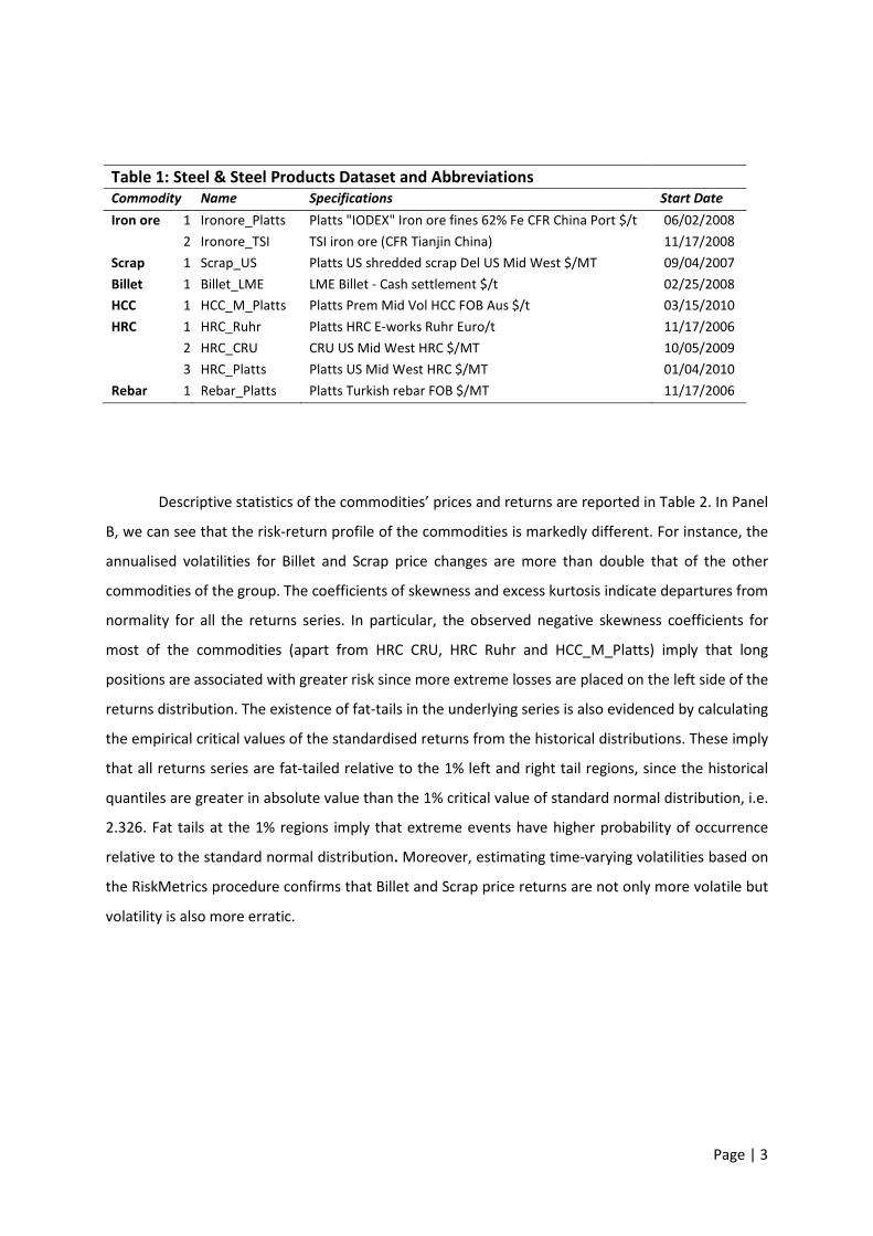
Table 1: Steel & Steel Products Dataset and Abbreviations
Commodity Name Specifications Start Date
Iron ore 1 Ironore_Platts Platts "IODEX" Iron ore fines 62% Fe CFR China Port $/t 06/02/2008
2 Ironore_TSI TSI iron ore (CFR Tianjin China) 11/17/2008
Scrap 1 Scrap_US Platts US shredded scrap Del US Mid West $/MT 09/04/2007
Billet 1 Billet_LME LME Billet - Cash settlement $/t 02/25/2008
HCC 1 HCC_M_Platts Platts Prem Mid Vol HCC FOB Aus $/t 03/15/2010
HRC 1 HRC_Ruhr Platts HRC E-works Ruhr Euro/t 11/17/2006
2 HRC_CRU CRU US Mid West HRC $/MT 10/05/2009
3 HRC_Platts Platts US Mid West HRC $/MT 01/04/2010
Rebar 1 Rebar_Platts Platts Turkish rebar FOB $/MT 11/17/2006
Descriptive statistics of the commodities’ prices and returns are reported in Table 2. In Panel
B, we can see that the risk-return profile of the commodities is markedly different. For instance, the
annualised volatilities for Billet and Scrap price changes are more than double that of the other
commodities of the group. The coefficients of skewness and excess kurtosis indicate departures from
normality for all the returns series. In particular, the observed negative skewness coefficients for
most of the commodities (apart from HRC CRU, HRC Ruhr and HCC_M_Platts) imply that long
positions are associated with greater risk since more extreme losses are placed on the left side of the
returns distribution. The existence of fat-tails in the underlying series is also evidenced by calculating
the empirical critical values of the standardised returns from the historical distributions. These imply
that all returns series are fat-tailed relative to the 1% left and right tail regions, since the historical
quantiles are greater in absolute value than the 1% critical value of standard normal distribution, i.e.
2.326. Fat tails at the 1% regions imply that extreme events have higher probability of occurrence
relative to the standard normal distribution. Moreover, estimating time-varying volatilities based on
the RiskMetrics procedure confirms that Billet and Scrap price returns are not only more volatile but
volatility is also more erratic.
Page | 4
Figure 1 displays the volatility processes for different product prices1. Time variation in the
volatility dynamics is confirmed, whereas the high volatility levels the industry experienced from the
second half of 2008 and 2009 are also apparent. However, in the short term, we can note
divergences in the processes, and, whether increases in volatility are transmitted to all markets is
not obvious. The average correlation of the time series of volatilities is around 30% excluding CRU US
1 RiskMetrics uses a weighted average of the estimated volatility and the last change in price at any point in
time to estimate volatility. This is a simple Exponentially Weighted Moving Average (EWMA) procedure which
essentially assigns different weights to each observation. In particular, the basic EWMA specification allows
more recent observations to carry largest weights whereas weights associated with previous observations
decline exponentially over time. Thus more recent observations have a stronger impact on volatility. Let be
the squared returns (daily) and λ the weight/decay factor. The decay factor could be estimated but usually it is
set at 0.94 as recommended by RiskMetrics. Then, the standard EWMA model of RiskMetrics can be
represented as :
2221
2
0
121 )1()1( tttt
j
jt RR λλσσλλσ −+=⇒−= +
∞
=
−+ ∑
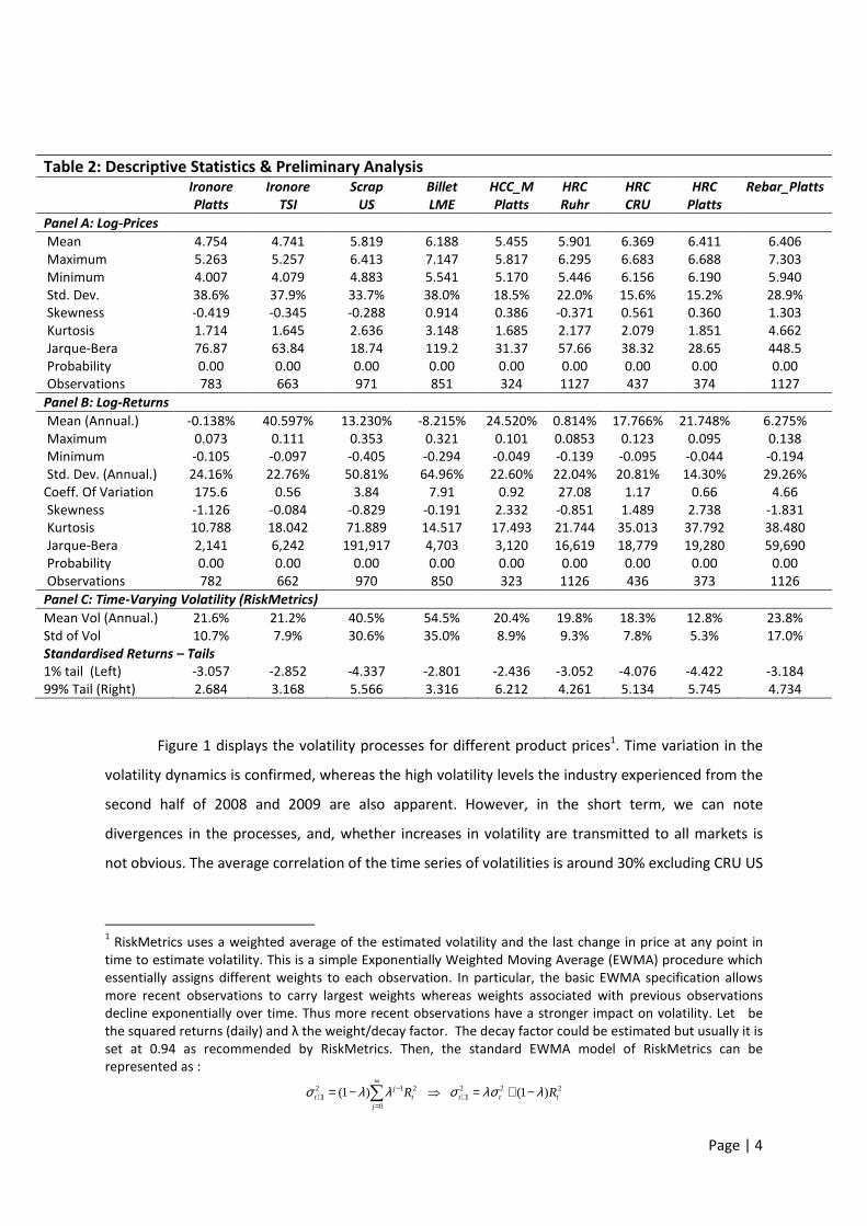
Table 2: Descriptive Statistics & Preliminary Analysis Ironore
Platts
Ironore
TSI
Scrap
US
Billet
LME
HCC_M
Platts
HRC
Ruhr
HRC
CRU
HRC
Platts
Rebar_Platts
Panel A: Log-Prices
Mean 4.754 4.741 5.819 6.188 5.455 5.901 6.369 6.411 6.406
Maximum 5.263 5.257 6.413 7.147 5.817 6.295 6.683 6.688 7.303
Minimum 4.007 4.079 4.883 5.541 5.170 5.446 6.156 6.190 5.940
Std. Dev. 38.6% 37.9% 33.7% 38.0% 18.5% 22.0% 15.6% 15.2% 28.9%
Skewness -0.419 -0.345 -0.288 0.914 0.386 -0.371 0.561 0.360 1.303
Kurtosis 1.714 1.645 2.636 3.148 1.685 2.177 2.079 1.851 4.662
Jarque-Bera 76.87 63.84 18.74 119.2 31.37 57.66 38.32 28.65 448.5
Probability 0.00 0.00 0.00 0.00 0.00 0.00 0.00 0.00 0.00
Observations 783 663 971 851 324 1127 437 374 1127
Panel B: Log-Returns
Mean (Annual.) -0.138% 40.597% 13.230% -8.215% 24.520% 0.814% 17.766% 21.748% 6.275%
Maximum 0.073 0.111 0.353 0.321 0.101 0.0853 0.123 0.095 0.138
Minimum -0.105 -0.097 -0.405 -0.294 -0.049 -0.139 -0.095 -0.044 -0.194
Std. Dev. (Annual.) 24.16% 22.76% 50.81% 64.96% 22.60% 22.04% 20.81% 14.30% 29.26%
Coeff. Of Variation 175.6 0.56 3.84 7.91 0.92 27.08 1.17 0.66 4.66
Skewness -1.126 -0.084 -0.829 -0.191 2.332 -0.851 1.489 2.738 -1.831
Kurtosis 10.788 18.042 71.889 14.517 17.493 21.744 35.013 37.792 38.480
Jarque-Bera 2,141 6,242 191,917 4,703 3,120 16,619 18,779 19,280 59,690
Probability 0.00 0.00 0.00 0.00 0.00 0.00 0.00 0.00 0.00
Observations 782 662 970 850 323 1126 436 373 1126
Panel C: Time-Varying Volatility (RiskMetrics)
Mean Vol (Annual.) 21.6% 21.2% 40.5% 54.5% 20.4% 19.8% 18.3% 12.8% 23.8%
Std of Vol 10.7% 7.9% 30.6% 35.0% 8.9% 9.3% 7.8% 5.3% 17.0%
Standardised Returns – Tails
1% tail (Left) -3.057 -2.852 -4.337 -2.801 -2.436 -3.052 -4.076 -4.422 -3.184
99% Tail (Right) 2.684 3.168 5.566 3.316 6.212 4.261 5.134 5.745 4.734

Page | 5
Mid West HRC (black line in Figure 1) which seems to be negatively correlated to all other products (-
27% on average).
Furthermore, the fat tails and the high kurtosis in log returns (Table 2) mean that more of its
volatility can be explained by infrequent extreme events (excessive deviations from the mean –
relatively large shocks). This illustrates the uncertainty and risk underlying the return process in the
industry. As it has already been noted, the risk-return profile of the commodities is found to be
markedly different.
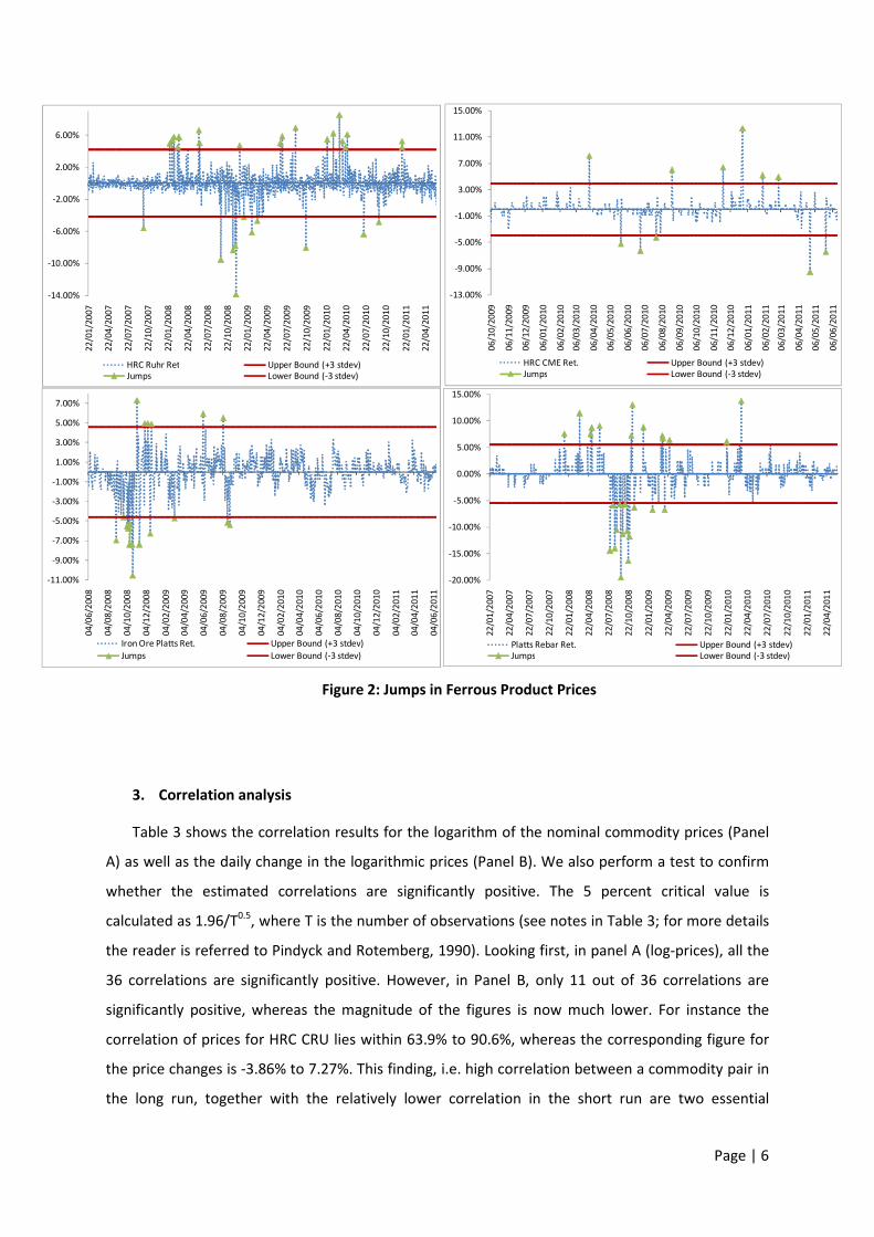
Figure 2 attempts to isolate some large shocks in different products. We define as a jump,
those returns with absolute values greater than three times the standard deviation (stdev) of the
returns of the series. The +/- stdev bounds are displayed in the graphs for illustration purposes (red
lines); jumps are also highlighted in green. Results show that extreme events in one market do not
necessarily occur simultaneously in all cases. Moreover, this is a first indication that
interdependencies during extreme events might not be frequent.
0%
20%
40%
60%
80%
100%
120%
140%
160%
180%
200%
13
/06
/20
08
13
/08
/20
08
13
/10
/20
08
13
/12
/20
08
13
/02
/20
09
13
/04
/20
09
13
/06
/20
09
13
/08
/20
09
13
/10
/20
09
13
/12
/20
09
13
/02
/20
10
13
/04
/20
10
13
/06
/20
10
13
/08
/20
10
13
/10
/20
10
13
/12
/20
10
13
/02
/20
11
13
/04
/20
11
13
/06
/20
11
% A
nn
ua
lise
d V
ola
tili
tie
s
RiskMetrics Volatilities in Ferrous Product Prices (lamda = 0.94)
Platts "IODEX" Iron ore Platts US shredded scrap LME Billet
Platts HRC E-works Ruhr CME US Mid West HRC Platts Turkish rebar
Figure 1: Conditional Annualised Volatilities in Ferrous Product Prices
Page | 6
3. Correlation analysis
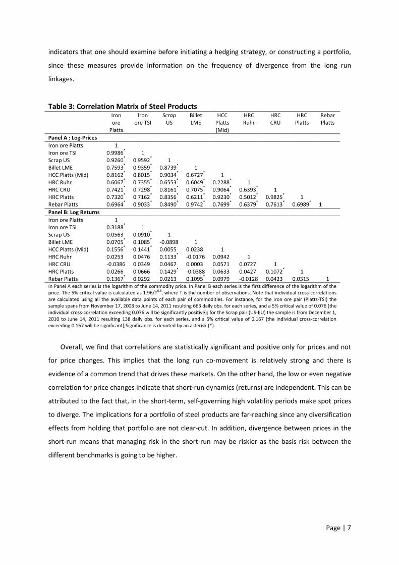
Table 3 shows the correlation results for the logarithm of the nominal commodity prices (Panel
A) as well as the daily change in the logarithmic prices (Panel B). We also perform a test to confirm
whether the estimated correlations are significantly positive. The 5 percent critical value is
calculated as 1.96/T0.5, where T is the number of observations (see notes in Table 3; for more details
the reader is referred to Pindyck and Rotemberg, 1990). Looking first, in panel A (log-prices), all the
36 correlations are significantly positive. However, in Panel B, only 11 out of 36 correlations are
significantly positive, whereas the magnitude of the figures is now much lower. For instance the
correlation of prices for HRC CRU lies within 63.9% to 90.6%, whereas the corresponding figure for
the price changes is -3.86% to 7.27%. This finding, i.e. high correlation between a commodity pair in
the long run, together with the relatively lower correlation in the short run are two essential
-11.00%
-9.00%
-7.00%
-5.00%
-3.00%
-1.00%
1.00%
3.00%
5.00%
7.00%
04
/06
/20
08
04
/08
/20
08
04
/10
/20
08
04
/12
/20
08
04
/02
/20
09
04
/04
/20
09
04
/06
/20
09
04
/08
/20
09
04
/10
/20
09
04
/12
/20
09
04
/02
/20
10
04
/04
/20
10
04
/06
/20
10
04
/08
/20
10
04
/10
/20
10
04
/12
/20
10
04
/02
/20
11
04
/04
/20
11
04
/06
/20
11
Iron Ore Platts Ret. Upper Bound (+3 stdev)
Jumps Lower Bound (-3 stdev)
-13.00%
-9.00%
-5.00%
-1.00%
3.00%
7.00%
11.00%
15.00%
06
/10
/20
09
06
/11
/20
09
06
/12
/20
09
06
/01
/20
10
06
/02
/20
10
06
/03
/20
10
06
/04
/20
10
06
/05
/20
10
06
/06
/20
10
06
/07
/20
10
06
/08
/20
10
06
/09
/20
10
06
/10
/20
10
06
/11
/20
10
06
/12
/20
10
06
/01
/20
11
06
/02
/20
11
06
/03
/20
11
06
/04
/20
11
06
/05
/20
11
06
/06
/20
11
HRC CME Ret. Upper Bound (+3 stdev)
Jumps Lower Bound (-3 stdev)
-20.00%
-15.00%
-10.00%
-5.00%
0.00%
5.00%
10.00%
15.00%
22
/01
/20
07
22
/04
/20
07
22
/07
/20
07
22
/10
/20
07
22
/01
/20
08
22
/04
/20
08
22
/07
/20
08
22
/10
/20
08
22
/01
/20
09
22
/04
/20
09
22
/07
/20
09
22
/10
/20
09
22
/01
/20
10
22
/04
/20
10
22
/07
/20
10
22
/10
/20
10
22
/01
/20
11
22
/04
/20
11
Platts Rebar Ret. Upper Bound (+3 stdev)Jumps Lower Bound (-3 stdev)
-14.00%
-10.00%
-6.00%
-2.00%
2.00%
6.00%
22
/01
/20
07
22
/04
/20
07
22
/07
/20
07
22
/10
/20
07
22
/01
/20
08
22
/04
/20
08
22
/07
/20
08
22
/10
/20
08
22
/01
/20
09
22
/04
/20
09
22
/07
/20
09
22
/10
/20
09
22
/01
/20
10
22
/04
/20
10
22
/07
/20
10
22
/10
/20
10
22
/01
/20
11
22
/04
/20
11
HRC Ruhr Ret Upper Bound (+3 stdev)Jumps Lower Bound (-3 stdev)
Figure 2: Jumps in Ferrous Product Prices
Page | 7
indicators that one should examine before initiating a hedging strategy, or constructing a portfolio,
since these measures provide information on the frequency of divergence from the long run
linkages.
Table 3: Correlation Matrix of Steel Products Iron
ore
Platts
Iron
ore TSI
Scrap
US
Billet
LME
HCC
Platts
(Mid)
HRC
Ruhr
HRC
CRU
HRC
Platts
Rebar
Platts
Panel A : Log-Prices
Iron ore Platts 1
Iron ore TSI 0.9986* 1
Scrap US 0.9260* 0.9592
* 1
Billet LME 0.7593* 0.9359
* 0.8739
* 1
HCC Platts (Mid) 0.8162* 0.8015
* 0.9034
* 0.6727
* 1
HRC Ruhr 0.6067* 0.7355
* 0.6553
* 0.6049
* 0.2288
* 1
HRC CRU 0.7421* 0.7298
* 0.8161
* 0.7075
* 0.9064
* 0.6393
* 1
HRC Platts 0.7320* 0.7162
* 0.8356
* 0.6211
* 0.9230
* 0.5012
* 0.9825
* 1
Rebar Platts 0.6964* 0.9033
* 0.8490
* 0.9742
* 0.7699
* 0.6379
* 0.7613
* 0.6989
* 1
Panel B: Log Returns
Iron ore Platts 1
Iron ore TSI 0.3188* 1
Scrap US 0.0563 0.0910* 1
Billet LME 0.0705* 0.1085
* -0.0898 1
HCC Platts (Mid) 0.1556* 0.1441
* 0.0055 0.0238 1
HRC Ruhr 0.0253 0.0476 0.1133* -0.0176 0.0942 1
HRC CRU -0.0386 0.0349 0.0467 0.0003 0.0571 0.0727 1
HRC Platts 0.0266 0.0666 0.1429* -0.0388 0.0633 0.0427 0.1072
* 1
Rebar Platts 0.1367* 0.0292 0.0213 0.1095
* 0.0979 -0.0128 0.0423 0.0315 1
In Panel A each series is the logarithm of the commodity price. In Panel B each series is the first difference of the logarithm of the
price. The 5% critical value is calculated as 1.96/T0.5
, where T is the number of observations. Note that individual cross-correlations
are calculated using all the available data points of each pair of commodities. For instance, for the Iron ore pair (Platts-TSI) the
sample spans from November 17, 2008 to June 14, 2011 resulting 663 daily obs. for each series, and a 5% critical value of 0.076 (the
individual cross-correlation exceeding 0.076 will be significantly positive); for the Scrap pair (US-EU) the sample is from December 1,
2010 to June 14, 2011 resulting 138 daily obs. for each series, and a 5% critical value of 0.167 (the individual cross-correlation
exceeding 0.167 will be significant);Significance is denoted by an asterisk (*).
Overall, we find that correlations are statistically significant and positive only for prices and not
for price changes. This implies that the long run co-movement is relatively strong and there is
evidence of a common trend that drives these markets. On the other hand, the low or even negative
correlation for price changes indicate that short-run dynamics (returns) are independent. This can be
attributed to the fact that, in the short-term, self-governing high volatility periods make spot prices
to diverge. The implications for a portfolio of steel products are far-reaching since any diversification
effects from holding that portfolio are not clear-cut. In addition, divergence between prices in the
short-run means that managing risk in the short-run may be riskier as the basis risk between the
different benchmarks is going to be higher.
Page | 8
Table 4: Average Rolling Correlation of HRC CRU with commodities
Based on 20Day
Correlation
Based on 40Day
Correlation
Based on 60Day
Correlation
Whole
Sample
����(��) ����(��) ����(��) ����(��) ����(��) ����(��)
Panel A: Correlation of Log-Prices
Ironore (Platts) 0.085* 0.282 0.146
* 0.499 0.198
* 0.542 0.742
*
Ironore (TSI) 0.078* 0.182 0.141
* 0.465 0.192
* 0.543 0.730
*
Scrap (US) 0.212* 0.394 0.393
* 0.564 0.392
* 0.582 0.816
*
Billet (LME) 0.097* 0.200 0.122
* 0.161 0.158
* 0.229 0.708
*
HCC Medium (Platts) 0.308* 0.530 0.463
* 0.722 0.463
* 0.723 0.906
*
HRC (Ruhr) 0.403* 0.632 0.536
* 0.755 0.538
* 0.775 0.639
*
HRC (Platts) 0.585* 0.733 0.806
* 0.863 0.806
* 0.864 0.983
*
Rebar (Platts) 0.174* 0.418 0.278
* 0.470 0.276
* 0.493 0.761
*
Panel B: Correlation of Volatilities (RiskMetrics)
Ironore (Platts) 0.048* 0.032 -0.032 -0.129 -0.018 -0.074 -0.476
Ironore (TSI) 0.034 -0.013 -0.114 -0.167 -0.091 -0.125 -0.569
Scrap (US) 0.192* 0.193 0.197
* 0.119 0.200
* 0.106 -0.255
Billet (LME) 0.180* 0.173 0.120
* 0.125 0.146
* 0.161 -0.176
HCC Medium (Platts) 0.039 -0.007 0.132* 0.143 0.133
* 0.144 0.435
*
HRC (Ruhr) 0.026 -0.017 0.109* 0.098 0.130
* 0.129 -0.171
HRC (Platts) 0.106* 0.056 0.154
* 0.196 0.153
* 0.195 0.544
*
Rebar (Platts) 0.092* 0.084 0.086
* 0.078 0.125
* 0.108 0.020
In Panel A (Panel B), ����(��)is the average time varying correlation coefficient between the log-price (conditional
volatility) of HRC CRU and the corresponding commodity log-price (conditional volatility); * indicates significance at the
5 percent level (the null hypothesis is that the average time-varying correlation is positive). ����(��) is the median
time varying correlation coefficient between the log-price (conditional volatility) of HRC CRU and the corresponding
commodity log-price (conditional volatility).
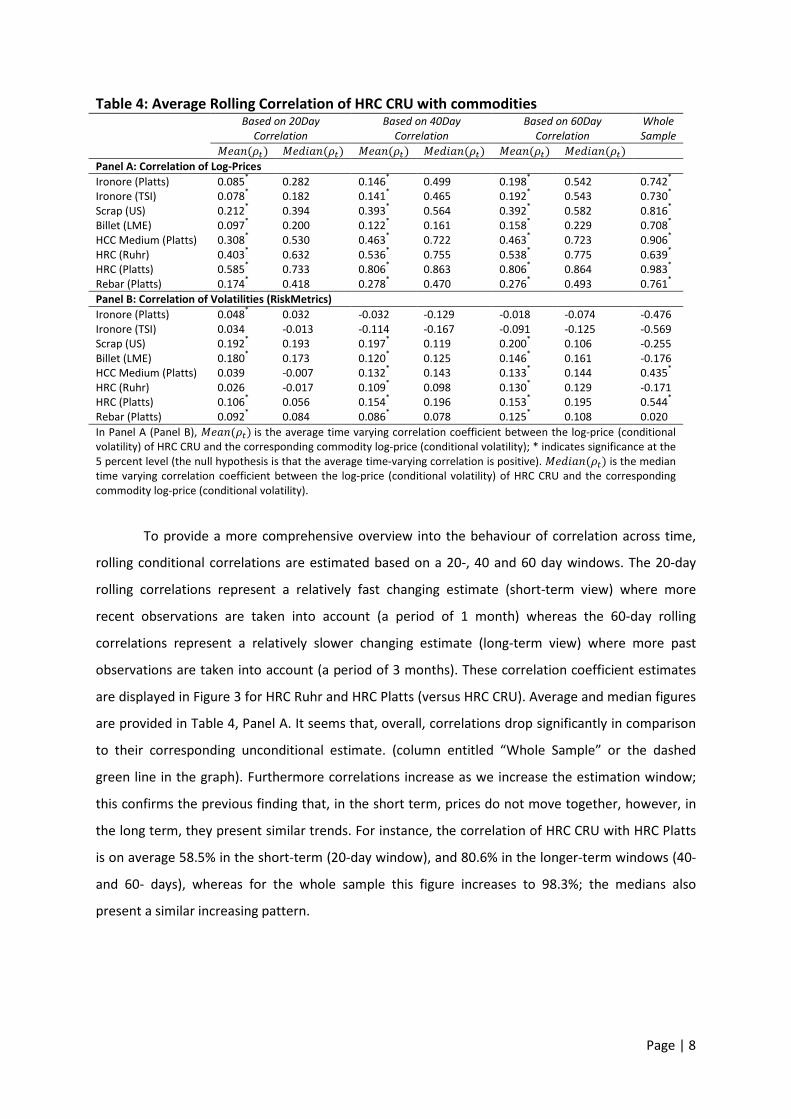
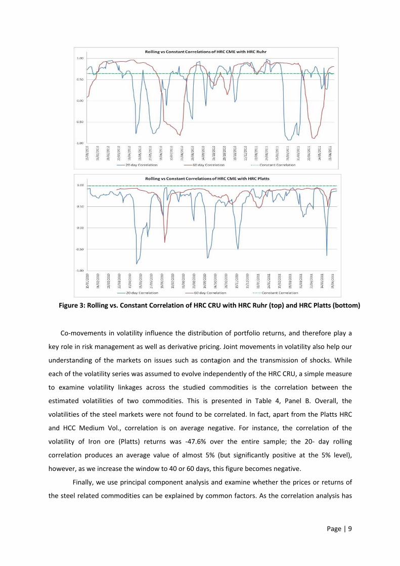
To provide a more comprehensive overview into the behaviour of correlation across time,
rolling conditional correlations are estimated based on a 20-, 40 and 60 day windows. The 20-day
rolling correlations represent a relatively fast changing estimate (short-term view) where more
recent observations are taken into account (a period of 1 month) whereas the 60-day rolling
correlations represent a relatively slower changing estimate (long-term view) where more past
observations are taken into account (a period of 3 months). These correlation coefficient estimates
are displayed in Figure 3 for HRC Ruhr and HRC Platts (versus HRC CRU). Average and median figures
are provided in Table 4, Panel A. It seems that, overall, correlations drop significantly in comparison
to their corresponding unconditional estimate. (column entitled “Whole Sample” or the dashed
green line in the graph). Furthermore correlations increase as we increase the estimation window;
this confirms the previous finding that, in the short term, prices do not move together, however, in
the long term, they present similar trends. For instance, the correlation of HRC CRU with HRC Platts
is on average 58.5% in the short-term (20-day window), and 80.6% in the longer-term windows (40-
and 60- days), whereas for the whole sample this figure increases to 98.3%; the medians also
present a similar increasing pattern.
Page | 9
Co-movements in volatility influence the distribution of portfolio returns, and therefore play a
key role in risk management as well as derivative pricing. Joint movements in volatility also help our
understanding of the markets on issues such as contagion and the transmission of shocks. While
each of the volatility series was assumed to evolve independently of the HRC CRU, a simple measure
to examine volatility linkages across the studied commodities is the correlation between the
estimated volatilities of two commodities. This is presented in Table 4, Panel B. Overall, the
volatilities of the steel markets were not found to be correlated. In fact, apart from the Platts HRC
and HCC Medium Vol., correlation is on average negative. For instance, the correlation of the
volatility of Iron ore (Platts) returns was -47.6% over the entire sample; the 20- day rolling
correlation produces an average value of almost 5% (but significantly positive at the 5% level),
however, as we increase the window to 40 or 60 days, this figure becomes negative.
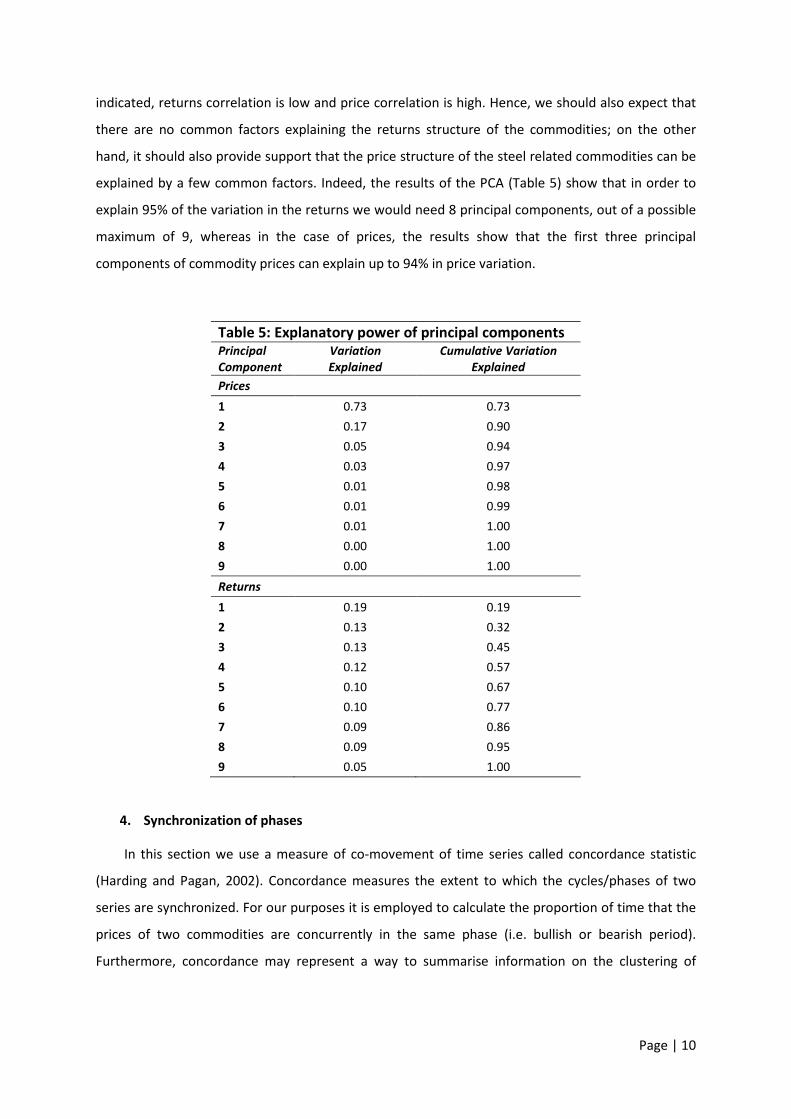
Finally, we use principal component analysis and examine whether the prices or returns of
the steel related commodities can be explained by common factors. As the correlation analysis has
Figure 3: Rolling vs. Constant Correlation of HRC CRU with HRC Ruhr (top) and HRC Platts (bottom)
Page | 10
indicated, returns correlation is low and price correlation is high. Hence, we should also expect that
there are no common factors explaining the returns structure of the commodities; on the other
hand, it should also provide support that the price structure of the steel related commodities can be
explained by a few common factors. Indeed, the results of the PCA (Table 5) show that in order to
explain 95% of the variation in the returns we would need 8 principal components, out of a possible
maximum of 9, whereas in the case of prices, the results show that the first three principal
components of commodity prices can explain up to 94% in price variation.
Table 5: Explanatory power of principal components
Principal
Component
Variation
Explained
Cumulative Variation
Explained
Prices
1 0.73 0.73
2 0.17 0.90
3 0.05 0.94
4 0.03 0.97
5 0.01 0.98
6 0.01 0.99
7 0.01 1.00
8 0.00 1.00
9 0.00 1.00
Returns
1 0.19 0.19
2 0.13 0.32
3 0.13 0.45
4 0.12 0.57
5 0.10 0.67
6 0.10 0.77
7 0.09 0.86
8 0.09 0.95
9 0.05 1.00
4. Synchronization of phases
In this section we use a measure of co-movement of time series called concordance statistic
(Harding and Pagan, 2002). Concordance measures the extent to which the cycles/phases of two
series are synchronized. For our purposes it is employed to calculate the proportion of time that the
prices of two commodities are concurrently in the same phase (i.e. bullish or bearish period).
Furthermore, concordance may represent a way to summarise information on the clustering of
Page | 11
turning points, i.e. whether bullish phases for different commodities turn into bearish phases at the
same time.
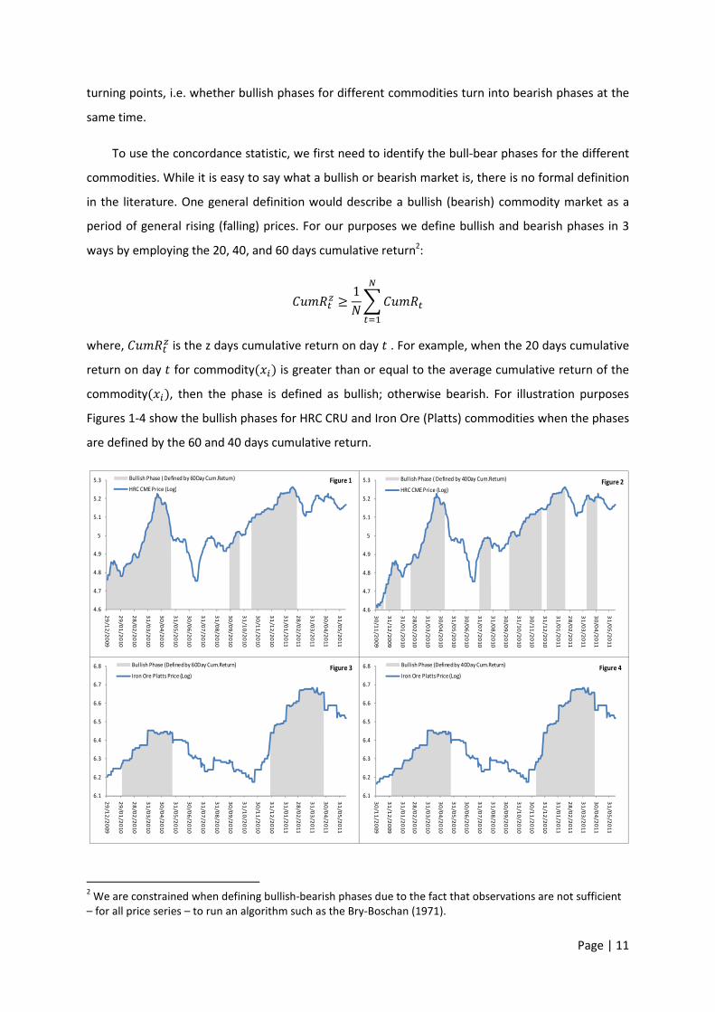
To use the concordance statistic, we first need to identify the bull-bear phases for the different
commodities. While it is easy to say what a bullish or bearish market is, there is no formal definition
in the literature. One general definition would describe a bullish (bearish) commodity market as a
period of general rising (falling) prices. For our purposes we define bullish and bearish phases in 3
ways by employing the 20, 40, and 60 days cumulative return2:
� ���� ≥ 1��� ����
���
where, � ���� is the z days cumulative return on day � . For example, when the 20 days cumulative
return on day � for commodity(��) is greater than or equal to the average cumulative return of the
commodity(��), then the phase is defined as bullish; otherwise bearish. For illustration purposes
Figures 1-4 show the bullish phases for HRC CRU and Iron Ore (Platts) commodities when the phases
are defined by the 60 and 40 days cumulative return.
2 We are constrained when defining bullish-bearish phases due to the fact that observations are not sufficient
– for all price series – to run an algorithm such as the Bry-Boschan (1971).
4.6
4.7
4.8
4.9
5
5.1
5.2
5.3
29
/12
/20
09
29
/01
/20
10
28
/02
/20
10
31
/03
/20
10
30
/04
/20
10
31
/05
/20
10
30
/06
/20
10
31
/07
/20
10
31
/08
/20
10
30
/09
/20
10
31
/10
/20
10
30
/11
/20
10
31
/12
/20
10
31
/01
/20
11
28
/02
/20
11
31
/03
/20
11
30
/04
/20
11
31
/05
/20
11
Figure 1Bullish Phase ( Defined by 60Day Cum.Return)
HRC CME Price (Log)
6.1
6.2
6.3
6.4
6.5
6.6
6.7
6.8
29
/12
/20
09
29
/01
/20
10
28
/02
/20
10
31
/03
/20
10
30
/04
/20
10
31
/05
/20
10
30
/06
/20
10
31
/07
/20
10
31
/08
/20
10
30
/09
/20
10
31
/10
/20
10
30
/11
/20
10
31
/12
/20
10
31
/01
/20
11
28
/02
/20
11
31
/03
/20
11
30
/04
/20
11
31
/05
/20
11
Figure 3Bullish Phase (Defined by 60Day Cum.Return)
Iron Ore Platts Price (Log)
4.6
4.7
4.8
4.9
5
5.1
5.2
5.3
30
/11
/20
09
31
/12
/20
09
31
/01
/20
10
28
/02
/20
10
31
/03
/20
10
30
/04
/20
10
31
/05
/20
10
30
/06
/20
10
31
/07
/20
10
31
/08
/20
10
30
/09
/20
10
31
/10
/20
10
30
/11
/20
10
31
/12
/20
10
31
/01
/20
11
28
/02
/20
11
31
/03
/20
11
30
/04
/20
11
31
/05
/20
11
Figure 2Bullish Phase ( Defined by 40Day Cum.Return)
HRC CME Price (Log)
6.1
6.2
6.3
6.4
6.5
6.6
6.7
6.8
30
/11
/20
09
31
/12
/20
09
31
/01
/20
10
28
/02
/20
10
31
/03
/20
10
30
/04
/20
10
31
/05
/20
10
30
/06
/20
10
31
/07
/20
10
31
/08
/20
10
30
/09
/20
10
31
/10
/20
10
30
/11
/20
10
31
/12
/20
10
31
/01
/20
11
28
/02
/20
11
31
/03
/20
11
30
/04
/20
11
31
/05
/20
11
Figure 4Bullish Phase (Defined by 40Day Cum.Return)
Iron Ore Platts Price (Log)
Page | 12
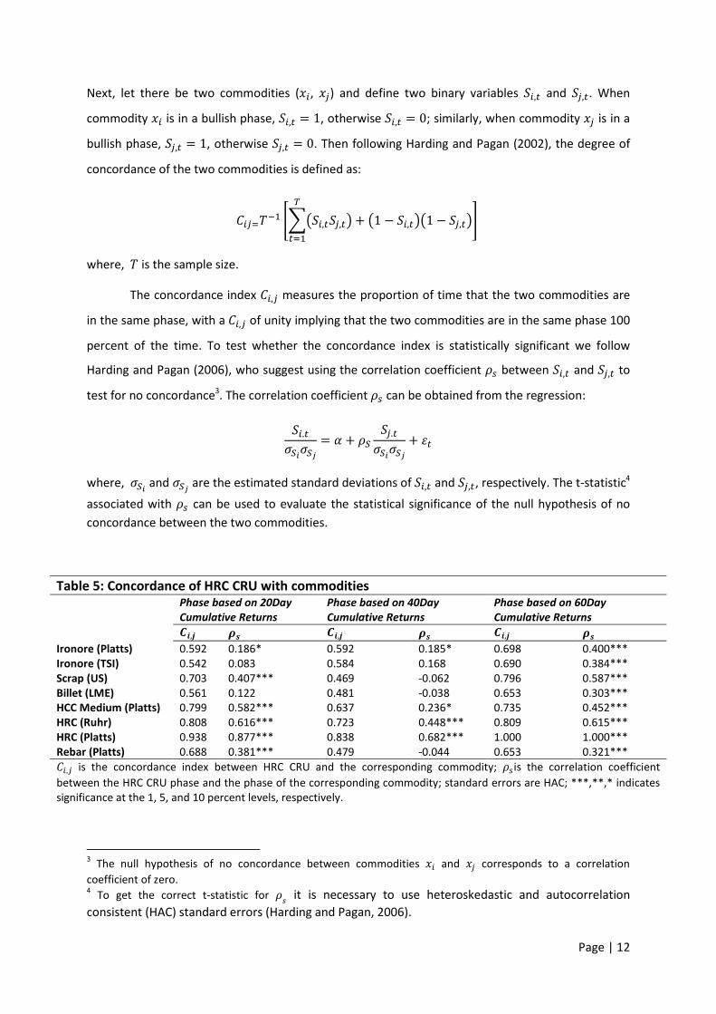
Next, let there be two commodities (��, ��) and define two binary variables ��,� and ��,�. When
commodity �� is in a bullish phase, ��,� = 1, otherwise ��,� = 0; similarly, when commodity �� is in a
bullish phase, ��,� = 1, otherwise ��,� = 0. Then following Harding and Pagan (2002), the degree of
concordance of the two commodities is defined as:
���� !� "�#��,���,�$ + #1 − ��,�$#1 − ��,�$'
���(
where, is the sample size.
The concordance index ��,� measures the proportion of time that the two commodities are
in the same phase, with a ��,� of unity implying that the two commodities are in the same phase 100
percent of the time. To test whether the concordance index is statistically significant we follow
Harding and Pagan (2006), who suggest using the correlation coefficient �) between ��,� and ��,� to
test for no concordance3. The correlation coefficient �) can be obtained from the regression:
��.�+,-+,. = / + �, ��.�+,-+,. + 0� where, +,- and +,. are the estimated standard deviations of ��,� and ��,�, respectively. The t-statistic4
associated with �) can be used to evaluate the statistical significance of the null hypothesis of no
concordance between the two commodities.
Table 5: Concordance of HRC CRU with commodities
Phase based on 20Day
Cumulative Returns
Phase based on 40Day
Cumulative Returns
Phase based on 60Day
Cumulative Returns
12,3 45 12,3 45 12,3 45 Ironore (Platts) 0.592 0.186* 0.592 0.185* 0.698 0.400***
Ironore (TSI) 0.542 0.083 0.584 0.168 0.690 0.384***
Scrap (US) 0.703 0.407*** 0.469 -0.062 0.796 0.587***
Billet (LME) 0.561 0.122 0.481 -0.038 0.653 0.303***
HCC Medium (Platts) 0.799 0.582*** 0.637 0.236* 0.735 0.452***
HRC (Ruhr) 0.808 0.616*** 0.723 0.448*** 0.809 0.615***
HRC (Platts) 0.938 0.877*** 0.838 0.682*** 1.000 1.000***
Rebar (Platts) 0.688 0.381*** 0.479 -0.044 0.653 0.321*** ��,� is the concordance index between HRC CRU and the corresponding commodity; �)is the correlation coefficient
between the HRC CRU phase and the phase of the corresponding commodity; standard errors are HAC; ***,**,* indicates
significance at the 1, 5, and 10 percent levels, respectively.
3 The null hypothesis of no concordance between commodities �� and �� corresponds to a correlation
coefficient of zero. 4 To get the correct t-statistic for �6 it is necessary to use heteroskedastic and autocorrelation
consistent (HAC) standard errors (Harding and Pagan, 2006).
Page | 13
Table 6 presents the concordance index ��,�, which allows us to examine if the price of HRC
CRU and the price of the rest of the commodities move together. Two interesting results can be
identified: a) when the bullish/bearish phase is defined by the 60 day cumulative return, the null
hypothesis of no concordance in the bilateral relationship of HRC CRU and the rest of the
commodities is rejected for any of the pairs; whereas, when the bullish/bearish phase is determined
according to the 40 day cumulative return, the null of no concordance is not rejected in some pairs;
2) the proportion of time that the prices of HRC CRU and another commodity are concurrently in the
same phase is greater when a phase is defined according to the 60 day cumulative return.
It seems that during short phases, it is difficult for commodities to be in the same phase. This
is evident by the statistically insignificant concordance indices during short-time phases; and the fact
that during long phases (defined by the 60 day cumulative return) concordance is higher and
statistically significant. Furthermore, HRC CRU appears to have the highest concordance with HRC
(Ruhr) and HRC (Platts), a logical result since we are dealing with the same commodity but different
price reference source. In respect to the rest of the HRC CRU commodity pairs, we can observe much
lower concordance during short phases and only the pairs of HRC CRU with HCC Medium (Platts) and
Iron Ore (Platts) being statistically significant.
Overall, concordance statistics for short and long phases give contradictory results leading to
the conclusion that, although commodities may move together through longer cycles, the co-
movement relationship may break down during shorter cycles.
5. Conclusion
The aim of this report was to identify whether there is variation in the correlation between
the various steel products and whether this relationship changes under different trading horizons.
The motivation for investigating this issues stems from the fact that although in the long-run
commodity prices reflect a common trend driven by the conditions of the World economy, over
shorter periods prices may exhibit greater independence in their behaviour. This is an important
issue for market participants as it implies that hedging policies may be less effective over short
periods of time due to the higher basis risk.
To identify these issues we investigate the correlation between the various steel products
and the raw materials used in their production process. The results indicate that whereas price
correlation is high, returns correlation for all the commodity pairs is generally low. As a result, we
Page | 14
could argue that in the long term, same steel commodities tend to move together, however, over
shorter periods of time, co-movement between steel related commodities is substantially lower.
The implications of these findings are as follows. Basis Risk can be quite high for hedging
short-term positions. In the absence of specialised steel futures contracts, hedging against price
fluctuations using existing contracts involves a cross-hedge, resulting in a critical disadvantage:
reduced hedging effectiveness. The fact that - in the short term - there seems to be a certain degree
of independence, implies that the industry’s risk factors affect steel-related commodities in a non-
uniform way and this in turn highlights the need for individual financial solutions i.e. more products,
adequate to cover the needs of all parts of the supply chain. Basis risk, arising from differences in the
derivative contract written and the actual underlying asset could prove disastrous in hedging due to
fragile correlation structure. The steeper the basis risk, the larger the disincentive to hedge. In other
words specialist hedging tools may be required to hedge short-term positions.
Even for longer-term positions, basis risk can also be high due to the short-term fluctuations
in prices. There is evidence that wide variations in steel price differentials are common and a single
unified price cannot serve the industry accurately. Even if two commodities move in proximity to
one another, extreme short term variations can be a very challenging task to deal with. In fact, large
basis risk can be equally problematic to unhedged positions (or even worse, since it falsely creates a
deceptive sense of security). Ignoring the stochastic behaviour of the correlation of steel prices and,
most importantly, the cash flow requirements to support potential day-to-day losses of a hedging
scheme for long term positions, can lead to a debacle. The risk matrix function of the corporation
contains many risks apart from price risk such as basis, liquidity and credit risk.
Finally, the rationale for the existence of derivative markets is to facilitate price discovery
and offer the means to price and hedge risk. After the development of organised exchanges,
derivatives products expanded giving easy access to commodities. They increasingly gained
importance, motivating the entry of new financial players. However the steel industry is still on its
infancy regarding that matter. In markets characterised with uncertainty and risk, price risk exposure
can be and should be managed and controlled. In search for appropriate futures contracts it seems
that the correlations of products in the industry is not sufficiently strong and - with the exception of
some financial institutions, offering OTC derivatives products such as swaps and options- for many
products there is no tradable contract. Steel markets, have become increasingly volatile; fat-tails and
volatility clusters are a new feature in this market illustrating the importance of risk management in
the industry. As a result, the market surely will benefit from new financial products that will assist
participants to mitigate price risk across the supply chain.
Page | 15
References
Bry, G. and Boschan, C., 1971. Cyclical analysis of time series: Selected procedures and
computer programs, NBER: New York.
Buyuksahin, B., Haigh, M., and Robe,M., 2010. Commodities and equities: Ever a “market of
one”? Journal of Alternative Investments, 12, 76-95.
Harding, D., and Pagan, A., 2006. Synchronisation of Cycles, Journal of Econometrics, 132,
pp.59-79
Harding, D., and Pagan, A., 2002. Dissecting the cycle: a methodological investigation, Journal
of Monetary Economics, 49, pp.365-381.
Pindyck, R., and Rotemberg, J., 1990. The excess co-movement of commodity prices, Economic
Journal 100, 1173-1189.
Silvennoinen, A., and Thorp, S., 2010. Financialization, crisis and commodity correlation
dynamics, Working paper, Queensland University of Technology.
Tang, K., and Xiong, W., 2011. Index investment and financialization of commodities, Working
paper, Princeton University.