analysis of volatile organic compounds in water using static

Analysis of Volatile OrganicCompounds in Water Using StaticHeadspace-GC/MS

Abstract

A static headspace (SHS) method was optimized for the determination of volatile

organic compounds (VOCs) in water. Analysis was performed by GC/MS in simultane-

ous scan/SIM mode. Using the trace ion detection mode on a 5975C MSD equipped

with triple axis detection, "purge and trap" sensitivities can be obtained, combined

with the robustness and ease-of-use of static headspace.

Authors

Karine Jacq, Frank David, Pat Sandra

Research Institute for Chromatography

Pres. Kennedypark 26, B-8500 Kortrijk

Belgium

Matthew S. Klee

Agilent Technologies, Inc.

2850 Centerville Road

Wilmington, DE 19808

USA

Application NoteEnvironmental

2

closed with an aluminum crimp cap with PTFE/silicone sep-tum (P/N 5183-4477) using an electronic crimper (P/N 5184-3572).

An internal standard mixture of three deuterated VOCs wasused. The mixture was made from three individual solutionsof 1,2-dichloroethane-d4, toluene-d8, and chlorobenzene-d5(all from Supelco [Bellefonte, PA, USA], 2,000 ppm in meth-anol). The individual solutions were mixed and diluted inmethanol to 800 ng/mL. From this working solution, 10 µLwas spiked into each 10-mL sample aliquot, corresponding toan internal standard concentration of 800 ng/L (800 ppt).

In total, 60 target analytes were analyzed and are listed inTable 1. The target list corresponds to EPA Method 524.2 andis also typical of several EU methods.

Calibration was done by analyzing reference water blanksspiked with internal standards and mixtures of the target ana-lytes. Standard mixtures containing all 60 analytes are avail-able from Supelco or Dr Ehrenstorfer (Augsburg, Germany).For reference water, bottled drinking water (Evian) was usedwith the same salt and internal standards addition as used forthe samples. Bottled drinking water often offers better blankvalues than does HPLC grade water or Milli-Q water.

Calibration levels were between 45 and 1,250 ng/L. Thesewere obtained by spiking 10 µL of VOC standard solutions at45 to 1,250 ng/mL in methanol.

Instrumental Conditions

The analyses were performed on an Agilent 7890A GC/5975CMSD system. SHS was performed with an Agilent G1888 HSautosampler, equipped with a 1-mL sample loop. The SHSwas coupled to a split/splitless injection port. The carrier gasline entering the SSL inlet port was cut close to the inlet andthe long leg connected to the carrier gas inlet port on theG1888. The transfer line from the G1888 was connected witha stainless steel zero dead volume union on the tubing endclose to the SSL inlet.

The 5975C MSD was operated in simultaneous SIM/SCANmode with the trace ion detection mode switched on. TheMSD was also equipped with the triple axis detector (TAD)option.

Introduction

The determination of volatile organic compounds (VOCs) inenvironmental samples is mostly performed using either staticheadspace (SHS) or purge and trap (P&T) extraction. Bothcombine separation by gas chromatography (GC) with detec-tion by mass spectrometry (MS). P&T (also called dynamicheadspace) is based on an exhaustive extraction processwhere, ideally, all solutes present in the sample are extractedcompletely, concentrated in an adsorbent trap, and then ther-mally desorbed from the trap to introduce sample to theGC/MS for analysis. In contrast, SHS establishes an equilibri-um between the solid or liquid sample and the gas or head-space phase above it in a sealed vial. A portion of the head-space is transferred to the GC/MS for analysis via a valvewith a sample loop. In principle, because of exhaustive sam-pling, P&T is more sensitive than SHS and is preferred foranalysis of sub-ppb (ng/L) VOCs in drinking water and surfacewater. However, P&T autosamplers are more complicated torun and maintain than are SHS autosamplers. SHS offershigher robustness and fewer problems related to carryover,cross-contamination, foam formation (due to the presence ofdetergents), and water management (trapping problems). Inmany routine laboratories, there is high interest in efforts toimprove instrumentation to the point where SHS analyzesVOCs at the necessary regulatory limits.

Recent developments in GC/MS hardware have resulted inhigher sensitivity and lower detection limits, thereby allowingSHS to be considered for drinking and surface water analyses.In addition, faster electronics allow the use of simultaneousscan/SIM methods and fast GC separation, while maintainingenough data points for accurate peak detection and quantification.

In this application note it is shown that by using a state-of-the-art GC/MS system and optimized SHS conditions, P&Tsensitivities can be obtained, while maintaining all of the clas-sic advantages of static headspace in terms of ease of useand robustness.

Experimental Conditions

Sample Preparation

Analyses were performed using 10-mL water samples.Samples were placed in a 20-mL headspace vial (P/N 5182-0837) containing 7 g sodium sulfate. The samples were spikedwith an internal standard solution. The vials were tightly

3

The experimental conditions can be summarized as follows:

SHS Incubation: 10 min at 70 °C, high shake mode

Pressurization: 0.15 min, 20 kPa

Loop: 1 mL, 120 °C, 0.5 min fill time, 0.1 min equilibration time transfer line 120 °C, 0.5 min injection time

GC

Inlet: Split/splitless, 250 °C, split 1/10, headspace liner (P/N 5183-4709)

Column: DB-624, 20 m × 0.18 mm × 1 µm (J & W 121-1324)

Gas: He, constant pressure (95 kPa)

Oven: 40 °C (5 min) → 180 °C @ 8 °C/min → 250 °C (0.17 min) @ 30 °C/min

Run time: 25-min run

Table 1. SIM Windows, Retention Times, and Ions for Quantification

Peak RT Start time Dwell Targetno Name CAS (min) window time (ms) IS ion Qualifiers

1 Dichlorodifluoromethane 75-71-8 1.31 0.00 70 1 85 87 50

2 Chloromethane 74-87-3 1.45 1 50 52

3 Vinylchloride 75-01-4 1.55 1 62 64

4 Bromomethane 74-83-9 1.80 1.80 100 1 94 96

5 Chloroethane 75-00-3 1.89 1 64 49

6 Fluorotrichloromethane 75-69-4 2.12 2.10 100 1 101 103 66

7 1,1-dichloroethene 75-35-4 2.62 2.55 100 1 96 61 98

8 Dichloromethane 75-09-2 3.17 3.10 100 1 49 84 86

9 1,2-dichloroethene Z 156-60-5 3.50 3.45 100 1 61 96 98

10 1,1-dichloroethane 75-34-3 4.11 4.00 100 1 63 83 98

11 2,2-dichloropropane 594-20-7 5.07 4.60 70 1 77 41

12 1,2-dichloroethene E 156-59-2 5.13 1 61 96 98

13 Bromochloromethane 74-97-5 5.55 5.50 70 1 49 130

14 Trichloromethane 67-66-3 5.75 1 83 47

15 1,1,1-trichloroethane 71-55-6 6.02 1 97 61

16 Tetrachloromethane 56-23-5 6.32 6.25 70 1 119 117 82

17 1,1-dichloro-1-propene 563-58-6 6.35 1 75 39 110

IS1 1,2-dichloroethane d4 6.72 IS1 65 102

18 Benzene 71-43-2 6.73 6.55 70 2 78 52

19 1,2-dichloroethane 107-06-2 6.79 1 98 62

20 Trichloroethene 79-01-6 7.98 7.40 100 1 132 95 130

21 1,2-dichloropropane 78-87-5 8.40 8.30 100 1 63 76 112

22 Dibromomethane 74-95-3 8.61 1 174 93 79

23 Bromodichloromethane 75-27-4 8.97 8.85 100 1 83 47 129

24 1,3-dichloropropene Z 542-75-6 9.82 9.50 100 1 75 39 110

IS2 Toluene d8 10.30 10.10 70 IS2 98 100 70

25 Toluene 108-88-3 10.42 2 91 92 65

26 1,3-dichloropropene E 542-75-6 10.93 10.68 100 1 75 39 110

MS (5975C Inert, Agilent)

Transfer line: 300 °C

Scan: 0 to 2 min: 45 to 300 m/z, 2 to 25 min: 33 to 300 m/z

SIM: See Table 1

Triple Axis Detector (G3392A upgrade kit)

The method was locked on toluene at 10.42 min. All the datashown correspond to the SIM chromatograms.

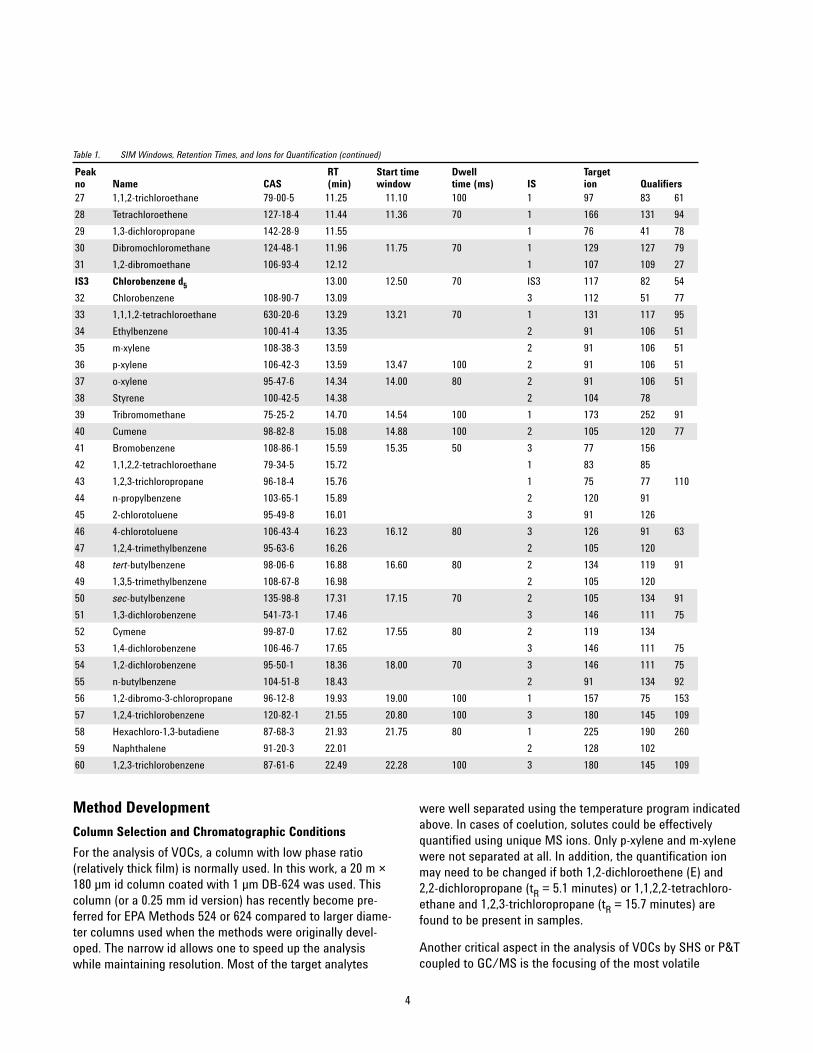
27 1,1,2-trichloroethane 79-00-5 11.25 11.10 100 1 97 83 61

28 Tetrachloroethene 127-18-4 11.44 11.36 70 1 166 131 94

29 1,3-dichloropropane 142-28-9 11.55 1 76 41 78

30 Dibromochloromethane 124-48-1 11.96 11.75 70 1 129 127 79

31 1,2-dibromoethane 106-93-4 12.12 1 107 109 27

IS3 Chlorobenzene d5 13.00 12.50 70 IS3 117 82 54

32 Chlorobenzene 108-90-7 13.09 3 112 51 77

33 1,1,1,2-tetrachloroethane 630-20-6 13.29 13.21 70 1 131 117 95

34 Ethylbenzene 100-41-4 13.35 2 91 106 51

35 m-xylene 108-38-3 13.59 2 91 106 51

36 p-xylene 106-42-3 13.59 13.47 100 2 91 106 51

37 o-xylene 95-47-6 14.34 14.00 80 2 91 106 51

38 Styrene 100-42-5 14.38 2 104 78

39 Tribromomethane 75-25-2 14.70 14.54 100 1 173 252 91

40 Cumene 98-82-8 15.08 14.88 100 2 105 120 77

41 Bromobenzene 108-86-1 15.59 15.35 50 3 77 156

42 1,1,2,2-tetrachloroethane 79-34-5 15.72 1 83 85

43 1,2,3-trichloropropane 96-18-4 15.76 1 75 77 110

44 n-propylbenzene 103-65-1 15.89 2 120 91

45 2-chlorotoluene 95-49-8 16.01 3 91 126

46 4-chlorotoluene 106-43-4 16.23 16.12 80 3 126 91 63

47 1,2,4-trimethylbenzene 95-63-6 16.26 2 105 120

48 tert-butylbenzene 98-06-6 16.88 16.60 80 2 134 119 91

49 1,3,5-trimethylbenzene 108-67-8 16.98 2 105 120

50 sec-butylbenzene 135-98-8 17.31 17.15 70 2 105 134 91

51 1,3-dichlorobenzene 541-73-1 17.46 3 146 111 75

52 Cymene 99-87-0 17.62 17.55 80 2 119 134

53 1,4-dichlorobenzene 106-46-7 17.65 3 146 111 75

54 1,2-dichlorobenzene 95-50-1 18.36 18.00 70 3 146 111 75

55 n-butylbenzene 104-51-8 18.43 2 91 134 92

56 1,2-dibromo-3-chloropropane 96-12-8 19.93 19.00 100 1 157 75 153

57 1,2,4-trichlorobenzene 120-82-1 21.55 20.80 100 3 180 145 109

58 Hexachloro-1,3-butadiene 87-68-3 21.93 21.75 80 1 225 190 260

59 Naphthalene 91-20-3 22.01 2 128 102

60 1,2,3-trichlorobenzene 87-61-6 22.49 22.28 100 3 180 145 109

4

Method Development

Column Selection and Chromatographic Conditions

For the analysis of VOCs, a column with low phase ratio (relatively thick film) is normally used. In this work, a 20 m ×180 µm id column coated with 1 µm DB-624 was used. Thiscolumn (or a 0.25 mm id version) has recently become pre-ferred for EPA Methods 524 or 624 compared to larger diame-ter columns used when the methods were originally devel-oped. The narrow id allows one to speed up the analysiswhile maintaining resolution. Most of the target analytes

were well separated using the temperature program indicatedabove. In cases of coelution, solutes could be effectivelyquantified using unique MS ions. Only p-xylene and m-xylenewere not separated at all. In addition, the quantification ionmay need to be changed if both 1,2-dichloroethene (E) and2,2-dichloropropane (tR = 5.1 minutes) or 1,1,2,2-tetrachloro-ethane and 1,2,3-trichloropropane (tR = 15.7 minutes) arefound to be present in samples.

Another critical aspect in the analysis of VOCs by SHS or P&Tcoupled to GC/MS is the focusing of the most volatile

Peak RT Start time Dwell Targetno Name CAS (min) window time (ms) IS ion Qualifiers

Table 1. SIM Windows, Retention Times, and Ions for Quantification (continued)

5

Figure 1. Peak shape of very volatile compounds compared to less volatile compounds – Extracted Ion Chromatograms at m/e 85 (1. CCL2F2), m/e 50 (2. chloromethane), m/e 62 (3. vinylchloride), m/e 94 (4. bromomethane), and ions at m/e 91 and 106 (34. ethylbenzene and 35/36. m/p xylene).

(gaseous) solutes (first six eluters). If the transfer from thesampler (SHS or P&T) is too slow, their bandwidths are largeor distorted. Transfer and injection speeds can be increasedby increasing the split ratio, but the sensitivity decreases as aconsequence. A good compromise was found using a 1:10split ratio. The resulting peak widths obtained for a watersample spiked at the 300 ppt level are shown in Figure 1. Thepeaks for early peaks difluorodichloromethane, chloro-methane, vinylchloride, and bromomethane are broader thanfor the later-eluting (focused) analytes, such as ethylbenzeneand xylenes, but were still acceptable for good quantificationat the required detection limits.

Effect of Salt Addition

The sensitivity of an SHS method is limited by the concentra-tion of the VOC in the headspace. This concentration dependson the initial concentration in the water, the phase ratiobetween liquid phase and gas phase, and the water/air distri-bution constant. The last depends on solute characteristics(vapor pressure, water solubility), temperature, pressure, pH,and salt concentration.

To normalize the salt concentration (same concentration incalibration solutions and samples), a high concentration ofsalt (sodium chloride, sodium sulfate) is typically added tosaturate the sample.

The effect of salt addition is demonstrated in Figure 2 by com-paring the responses of the VOCs obtained by analyzing awater sample spiked at 300 ppt level with and without saltaddition. An average gain in sensitivity by a factor 2.2 wasobtained by addition of salt. The "salting-out effect" drivesthe VOCs into the headspace. For some solutes, such as 1,2-bromo-3-chloropropane, which has a lower response inMS, the gain was almost a factor of 4.

Figure 2 shows overlaid SIM chromatograms for some early-eluting (highly volatile) solutes (Figure 2a) and midelutingones (Figure 2b). The gain factor for the most volatile solutes(gases: chloromethane to vinylchloride) is small for some (= 1.5), but is larger for the mideluters (gain is a factor < 2.5).

6

SHS Conditions

Incubation Time

Since SHS is an equilibrium technique, the equilibration timeplays an important role. Maximum sensitivity is obtained ifequilibrium is reached between the concentration of thesolutes in the sample and in the headspace gas phase. Testswere made using a 10-mL water sample spiked at 300 pptlevel. Headspace injections were performed after equilibrationtimes between 10 and 60 minutes (using 80 °C equilibrationtemperature, high shaking).

No significant difference in peak areas was observed for thedifferent VOCs, indicating that equilibrium is reached for the10-mL sample using the high-shaking mode on the G1888 inless than 10 minutes. Therefore, an equilibration time of 10 minutes was selected for further work.

Incubation Temperature

The sample-headspace equilibrium is also influenced by thetemperature. Seven experiments with increasing incubationtemperature from 40 to 100 °C in 10 °C increments were per-formed (10-minute equilibration time, vial pressure: 48 kPa).

In general it is expected that a higher temperature willincrease the concentration of the solutes in the headspaceand consequently will increase the response in GC/MS analysis.

From the experiments, however, some interesting observa-tions can be made. The responses (peak areas) for someselected solutes are plotted versus equilibration temperaturein Figure 3. Vinylchloride was selected as representative forthe high-volatility (early-eluting) VOCs, benzene was selectedas representative for a medium-volatility (mideluting) VOC,and 1,2,3-trichlorobenzene as a representative for the late-eluting, low-volatility VOCs.

As can be seen from the plots, the high-volatility solutesbehave slightly differently from the others. Between 40 and70 °C, the response obtained for vinylchloride is nearly con-stant. At temperatures higher than 70 °C, the response drops.The same behavior was observed for the other early-elutingsolutes (for example, dichlorodifluoromethane,chloromethane, bromomethane, chloroethane and fluo-rotrichloromethane). For these solutes, static headspaceextraction at low equilibration temperatures is already efficient.

For medium- and low-volatility solutes, the analytical sensitiv-ity maximized at 70 °C. For all solutes, including the high-volatility analytes, responses decreased by 50 to 60 percentas the equilibrium temperature increased from 70 to 100 °C.This is probably caused by increased vial pressure leading tohigher dilution during sample loading (decompression) in theheadspace sampler.

Salt

No salt1

2 3

45

6

7

1.20 1.40 1.60 1.80 2.00 2.20 2.40 2.60 2.80

150

200

250

300

350

400

450

500

550

600

650

700

750

800

850

Time Time

Abu

ndan

ce

Salt

No salt

13

14

15

16+17

IS1+18+19

5.60 5.80 6.00 6.20 6.40 6.60 6.80 7.00 7.20

300

350

400

450

500

550

600

650

700

750

Abu

ndan

ce

Figure 2. Effect of salt addition on response, water spiked at 300 ppt. See Tables 1 and 2 for peak identification.

7

The higher response obtained at 70 °C in comparison to equi-libration at 40 °C is illustrated for the solutes eluting in the2.5- to 9-minute elution window (eluting between dichloro-ethene and bromodichloromethane) in Figure 4a. In Figure 4b,the chromatograms obtained at 70 and 100 °C (similar elutionwindow as in Figure 4a) are compared. The decrease inresponse at 100 °C is clear and, moreover, an increase in

0

200

400

600

800

1000

1200

40 50 60 70 80 90 100

Incubation temperature (°C)

Incubation temperature influence

Vinyl chloride

Benzene

1,2,3-trichlorobenzene

Res

pons

e

Figure 3. Influence of SHS incubation temperature on response for vinylchloride (early eluter), benzene (mideluter), and 1,2,3-trichlorobenzene (late eluter).

background level is observed. This is probably due to theintroduction of a higher amount of water (as vapor) duringheadspace injection.

For these reasons, 70 °C was selected as the optimum equilibration temperature.

8

Abu

ndan

ce

150

200

250

300

350

400

450

500

550

600

650

700

750

Time

2.50 3.00 3.50 4.00 4.50 5.00 5.50 6.00 6.50 7.00 7.50 8.00 8.50 9.00

7

89

10

11+12

13

14

15

16+17

IS1+18+19

20

21

22

23

70 °C

40 °C

Figure 4a. Overlay of SIM chromatograms obtained by SHS GC/MS using incubation temperatures of 40 and 70 °C. See Tables 1 and 2 for peak identification.

Abu

ndan

ce

Time

2.50 3.00 3.50 4.00 4.50 5.00 5.50 6.00 6.50 7.00 7.50

150

200

250

300

350

400

450

500

550

600

650

700

7

89

10

11+12

13

14

15

16+17

IS1+18+19

100 °C

70 °C

Figure 4b. Overlay of SIM chromatograms obtained by SHS GC/MS using incubation temperatures of 70 and 100 °C. See Tables 1 and 2 for peak identification.

9

Vial Pressure

After equilibrium, the vial is pressurized with carrier gas. Thepressurized headspace is vented to a gas sampling valve withsample loop for subsequent injection into the GC/MS foranalysis. The pressure provides a reproducible driving force tomove sample to the loop. Too little pressure will prevent arepresentative sample from filling the sample loop. Too muchpressure will result in excessive dilution of headspace, lower-ing the concentration of analytes and reducing analytical sen-sitivity. Since the optimal vial pressure is a function of severalvariables, such as vial size, sample temperature, and sampleloop volume, it should be optimized.

Six experiments were performed at 70 °C equilibrium temper-ature and 10-minute equilibrium time with increasing vialpressures from 0 to 100 kPa in 20-kPa increments. No signifi-cant difference in analyte sensitivity was observed for vialpressure settings between 0 and 40 kPa. At higher vial pres-sures, however, the response of all analytes dropped(response at 100 kPa was 30 percent lower than at 20 kPa vialpressure). A vial pressure of 20 kPa was selected as optimum.

Final Chromatogram

An example of a blank water sample spiked at 1,250 ppt level with all 60 solutes and the three internal standards (at 800 ppt) is shown in Figure 5.

Abu

ndan

ce

Time

78

9

10

11+12

13

14

15

16+17

IS1+18+1920

21

6

1

52

4

1.50 2.00 2.50 3.00 3.50 4.00 4.50 5.00 5.50 6.00 6.50 7.00 7.50 8.00 8.50

200

400

600

800

1000

1200

1400

1600

1800

2000

2200

3

Figure 5a. SIM chromatogram obtained by SHS GC/MS of water sample spiked at 1.25 ppb with VOCs. See Tables 1 and 2 for peak identification.

10

Time

Abu

ndan

ce

200

400

600

800

1000

1200

1400

1600

1800

2000

2200

27

28

29IS2

30

24

25

IS3+32

35+36

26

312223

41

3334

40

39

37+38

9.00 9.50 10.00 10.50 11.00 11.50 12.00 12.50 13.00 13.50 14.00 14.50 15.00 15.50

Figure 5b. SIM chromatogram obtained by SHS GC/MS of water sample spiked at 1.25 ppb with VOCs. See Tables 1 and 2 for peak identification.

Time

Abu

ndan

ce

200

400

600

800

1000

1200

1400

1600

1800

2000

2200

42+43

49

48

57

44

45

46+47

50

51

52+53

60

56

55

54

59

58

16.00 16.50 17.00 17.50 18.00 18.50 19.00 19.50 20.00 20.50 21.00 21.50 22.00 22.50

Figure 5c. SIM chromatogram obtained by SHS GC/MS of water sample spiked at 1.25 ppb with VOCs. See Tables 1 and 2 for peak identification.

11

Validation

Linearity

Linearity was tested on five levels (+ blank) between 45 and1,250 ppt. The correlation coefficients of the external stan-dard calibration curve were 0.99 on average. The correlationcoefficients for the internal standard method (plot of relativeareas versus relative concentration) for all solutes are givenin Table 2.

The linearity was better than 0.990 in all cases (average0.996), except for 1,2-dibromo-3-chloropropane (r² = 0.966),which gives a lower response in MS.

The linearity was also calculated as %RSD in relativeresponse factors over the entire calibration range. The RSDvalues obtained in this range are also listed in Table 2. Forthree solutes, namely dichloromethane, trichloromethane(chloroform), and toluene, the lowest calibration points werenot taken into account, since in the blank analyses also sometraces of these solutes were present (due to lab contamination).

On average, the RSDs are around 10 to 15 percent (mean =13.6 percent), well below the 20 percent requirements speci-fied in EPA Method 524.2 (for P&T GC/MS).

Repeatability

Repeatability (n = 6) was tested at the 150-ppt level. Theaverage %RSD was 5.4 percent. For most solutes, even for thehigh-volatility analytes, the RSDs at this level were well below

10 percent. For some haloalkanes, which have lower MSresponses, higher values were observed, but still meetmethod requirements and are close to those achieved withP&T. For low-volatility solutes, such as aromatics (BTEX) andchloroaromatics, RSDs were excellent.

Limits of Detection (LODs)

Using trace ion detection (TID) mode (selected in methodsetup) in combination with a triple-axis detector (hardwareupgrade), improved signal-to noise values can be obtained asillustrated in Figure 6. A subset of the chromatogram isshown for a blank water sample spiked at 45 ppt, comparingstandard mode (Figure 6a) and TID ON (Figure 6b). Using TID,noise is reduced, resulting in better S/N ratio.

LODs were calculated for each compound at the 45-ppt level.Results are listed in Table 2. Typically, the LODs were ≤ 20 ppt. For most aromatics and chloroaromatics, LODs were≤ 10 ppt. For some haloalkanes and haloalkenes, the LOD wasbetween 20 and 50 ppt. 1,2-dichloroethane had the highestvalue at 136 ppt.

Regulatory limits, as included in EU Directive 98/83/EC ondrinking water, are 1 µg/L (1 ppb) for benzene, 10 µg/L (10 ppb) for trichloroethylene, and 0.5 µg/L (500 ppt) forvinylchloride. It is clear that the LODs obtained by this SHSGC/MS method are more than adequate to meet the EUmethod requirements (we achieved one to two orders of mag-nitude better LODs).

Time

Abu

ndan

ce

4.40 4.60 4.80 5.00 5.20 5.40 5.60 5.80 6.00 6.20 6.40 6.60 6.80 7.00 7.20 7.40 7.60 7.80260

280

300

320

340

360

Time

Abu

ndan

ce

4.40 4.60 4.80 5.00 5.20 5.40 5.60 5.80 6.00 6.20 6.40 6.60 6.80 7.00 7.20 7.40 7.60 7.80260

280

300

320

340

360

b

a

1

2

3

45 6

1

2

3

45 6

Figure 6. SIM chromatogram with MS in normal mode (top) or in TID ON mode (bottom) (water sample spiked at 45 ppt level).Peaks: 1. 2,2-dichloropropane+1,2-dichloroethene; 2. trichloromethane, 3. trichloroethane (1,1,1); 4. tetrachloromethane+1,1-dichloropropene; 5. benzene; and 6. dichloroethane.

12

Table. 2 Figures of Merit for VOC Analysis Using the New SHS GC/MS Method

r² RSD Peak 45 – 150 ppt RSD LODno Compounds RT Q Ion 1250 (n = 6) 45-1250 (ppt)

IS1 1,2-dichloroethane d4 6.72 65 / 3.3 / /

1 Dichlorodifluoromethane 1.31 85 0.996 2.6 13.5 24

2 Chloromethane 1.45 50 0.995 3.8 10.7 45

3 Vinyl chloride 1.55 62 0.998 5.7 6.4 15

4 Bromomethane 1.80 94 0.999 6.8 6.2 45

5 Chloroethane 1.89 64 0.999 2.4 5.7 27

6 Fluorotrichloromethane 2.12 101 0.998 1.8 18.5 6.3

7 1,1-dichloroethene 2.62 96 0.999 7.2 3.5 18

8 Dichloromethane 3.17 49 0.996 5.6 10.7* 20

9 1,2-dichloroethene trans 3.50 61 0.999 2.9 12.5 14

10 1,1-dichloroethane 4.11 63 0.999 0.7 9.5 12

11 2,2-dichloropropane 5.07 77 0.998 4.1 14.1 15

12 1,2-dichloroethene cis 5.13 61 1.000 4.2 8.4 23

13 Bromochloromethane 5.55 49 0.997 15.0 4.0 38

14 Trichloromethane 5.75 83 0.994 3.8 16.2* 10

15 1,1,1-trichloroethane 6.02 97 0.997 3.5 15.1 9.0

16 Tetrachloromethane 6.32 119 0.997 1.6 14.6 9.0

17 1,1-dichloro-1-propene 6.34 75 0.999 2.8 5.3 15

19 1,2-dichloroethane 6.79 98 0.992 11.2 5.2 136

20 Trichloroethene 7.98 132 0.997 5.0 6.9 10


22 Dibromomethane 8.61 174 0.996 11.3 8.2 20

23 Bromodichloromethane 8.97 83 0.999 6.7 4.9 21

24 1,3-dichloropropene cis 9.82 75 0.999 3.6 8.3 23

26 1,3-dichloropropene trans 10.93 75 0.999 19.3 13.4 28

27 1,1,2-trichloroethane 11.25 97 0.995 9.0 13.5 15

28 Tetrachloroethene 11.44 166 0.998 0.8 11.5 5.9


30 Dibromochloromethane 11.96 129 0.998 9.0 6.5 17

31 1,2-dibromoethane 12.12 107 0.994 7.6 12.0 20

33 1,1,1,2-tetrachloroethane 13.29 131 1.000 7.9 10.9 14

34 Tribromomethane 14.70 173 0.997 9.9 13.8 23

42 1,1,2,2-tetrachloroethane 15.72 83 0.992 9.3 12.9 14

43 1,2,3-trichloropropane 15.76 75 0.990 14.7 12.5 14

56 1,2-dibromo-3-chloropropane 19.93 157 0.966 19.4 9.5 47

58 Hexachloro-1,3-butadiene 21.93 225 0.993 3.7 16.7 5.9

IS2 Toluene d8 10.30 98 / 2.9 / /

18 Benzene 6.73 78 0.995 1.1 10.8 4.7

25 Toluene 10.42 91 0.991 2.5 8.8* 3.8

34 Ethylbenzene 13.35 91 0.999 2.8 7.5 4.5

35+36 p-xylene + m-xylene 13.59 91 0.998 2.3 16.4 3.0

37 o-xylene 14.34 106 0.999 7.9 13.1 13

38 Styrene 14.38 104 0.997 6.7 12.1 12

40 Cumene 15.08 105 0.999 3.2 15.4 4.2

44 n-propylbenzene 15.89 120 0.999 3.9 14.0 15

47 1,2,4-trimethylbenzene 16.26 105 0.999 3.8 10.1 7.9

13

Simultaneous Scan/SIM Mode

In the proposed method, the MS was operated in simultane-ous scan/SIM mode. The SIM mode resulted in high sensitivi-ty, while the scan mode can be used for confirmation ofsolute identity at 1-ppb or higher concentration levels (forsome solutes even at the 0.1-ppb level).

If needed, the scan data can also be used for identification ofnontarget sample components at levels above 1 ppb.

Table 2. Figures of Merit for VOC Analysis Using the New SHS GC/MS Method (continued)

r² RSD Peak 45 – 150 ppt RSD LODno Compounds RT Q Ion 1250 (n = 6) 45-1250 (ppt)

48 tert-butylbenzene 16.88 134 0.998 3.8 10.7 14

49 1,3,5-trimethylbenzene 16.98 105 0.998 4.1 10.8 7.6

50 sec-butylbenzene 17.31 105 0.997 4.2 6.1 4.1

52 Cymene 17.62 119 0.997 4.3 17.9 5.3

55 n-butylbenzene 18.43 91 0.998 3.8 16.5 5.8

59 Naphthalene 22.01 128 0.993 4.5 11.2 14

IS3 Chlorobenzene d5 13.00 117 / 2.5 / /

32 Chlorobenzene 13.09 112 0.995 1.5 16.2 6.4

41 Bromobenzene 15.59 77 0.995 6.8 13.5 17

45 2-chlorotoluene 16.01 91 0.999 4.5 17.7 7.6

46 4-chlorotoluene 16.23 126 0.999 2.5 14.3 9.4

51 1,3-dichlorobenzene 17.46 146 0.998 2.9 15.2 7.1



57 1,2,4-trichlorobenzene 21.55 180 0.998 6.1 13.2 11

60 1,2,3-trichlorobenzene 22.49 180 0.997 5.3 11.3 10

AVERAGE 0.996 5.4 13.6

*Contamination at lowest (45 ppt) level. RSDs listed are in the range of 150 to 1,250 ppt.

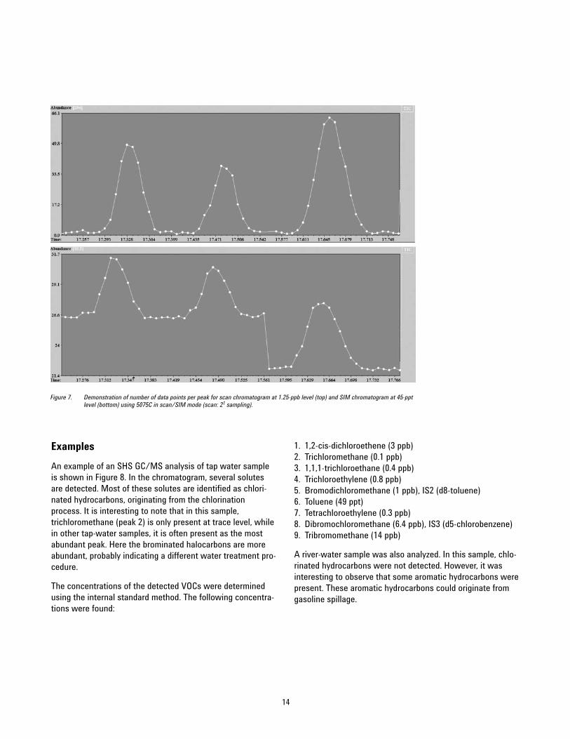
For SIM, dwell times of 50 to 100 ms were used and for scanmode, the sample rate was set at 21. This corresponds toabout 9 scans/s. In this way, more than five spectra are col-lected across the peak. This is illustrated in Figures 7a and 7b,showing the data points obtained for three late-eluting(focused) peaks (sec. butylbenzene, 1,3-dichlorobenzene, andcymene+1,4-dichlorobenzene) for a scan trace at 1-ppb leveland a SIM trace at 45-ppt level, respectively. (AMDIS wasused to highlight the data points).

14

Examples

An example of an SHS GC/MS analysis of tap water sampleis shown in Figure 8. In the chromatogram, several solutesare detected. Most of these solutes are identified as chlori-nated hydrocarbons, originating from the chlorinationprocess. It is interesting to note that in this sample,trichloromethane (peak 2) is only present at trace level, whilein other tap-water samples, it is often present as the mostabundant peak. Here the brominated halocarbons are moreabundant, probably indicating a different water treatment pro-cedure.

The concentrations of the detected VOCs were determinedusing the internal standard method. The following concentra-tions were found:

1. 1,2-cis-dichloroethene (3 ppb) 2. Trichloromethane (0.1 ppb) 3. 1,1,1-trichloroethane (0.4 ppb) 4. Trichloroethylene (0.8 ppb) 5. Bromodichloromethane (1 ppb), IS2 (d8-toluene) 6. Toluene (49 ppt) 7. Tetrachloroethylene (0.3 ppb) 8. Dibromochloromethane (6.4 ppb), IS3 (d5-chlorobenzene) 9. Tribromomethane (14 ppb)

A river-water sample was also analyzed. In this sample, chlo-rinated hydrocarbons were not detected. However, it wasinteresting to observe that some aromatic hydrocarbons werepresent. These aromatic hydrocarbons could originate fromgasoline spillage.

Figure 7. Demonstration of number of data points per peak for scan chromatogram at 1.25-ppb level (top) and SIM chromatogram at 45-ppt level (bottom) using 5075C in scan/SIM mode (scan: 21 sampling).

15

Abu

ndan

ce

5.00 6.00 7.00 8.00 9.00 10.00 11.00 12.00 13.00 14.00

1

2

3

4

5

IS2

6

7IS3

89

200

300

400

500

600

700

800

900

1000

1100

1200

1300

1400

1500

1600

1700

Time

Figure 8. Analysis of tap water using SHS GC/MS. Peaks: 1. 1,2-cis-dichloroethene (3 ppb); 2. 1,1,1-trichloroethane (0.4 ppb); 3. trichloromethane (0.1 ppb); 4. trichloroethylene (0.8 ppb); 5. bromodichloromethane (1 ppb), IS2 (d8-toluene); 6. toluene (49 ppt); 7. tetrachloroethylene (0.3 ppb); 8. dibromochloromethane (6.4 ppb), IS3 (d5-chlorobenzene); and 9. tribromomethane (14 ppb).

Abu

ndan

ce

1

2

3

4

5

6

7

40

50

60

70

80

90

100

Time

13.50 14.00 14.50 15.00 15.50 16.00 16.50 17.00 17.50 18.00 18.50

Figure 9. Extracted ion chromatograms obtained on river-water sample analyzed by SHS GC/MS. Peaks: 1. m/p xylene (13 ppt); 2. o. xylene (4 ppt); 3. 1,2,4-trimethylbenzene (39 ppt); 4. t.butylbenzene (5 ppt); 5. 1,3,5-trimethylbenzene (81 ppt); 6. C3-benzene isomer; and 7. cumene (88 ppt).

www.agilent.com/chem

Agilent shall not be liable for errors contained herein orfor incidental or consequential damages in connectionwith the furnishing, performance, or use of this material.

Information, descriptions, and specifications in this publi-cation are subject to change without notice.

© Agilent Technologies, Inc., 2008Published in the USADecember 9, 20085990-3285EN

Conclusions

A fast SHS GC/MS method was developed and validated for analysis of low-levelVOCs in water. Using the 5975C MSD with triple-axis detector, trace ion detectionmode, and simultaneous SIM/scan mode, LODs were one to two orders of magni-tude better than required by U.S. EPA and EU directives. Excellent repeatability androbustness can be obtained.

analysis of volatile organic compounds in water using static

Documents