analysis of variance (anova) - university of...
TRANSCRIPT

1
Analysis of Variance (ANOVA)
Two types of ANOVA tests:
Independent measures and Repeated measures
How can we Compare 3 means?: ANOVA Test compares three or more groups or conditions For ANOVA we work with variances instead of means
!
X 1 = 20X 2 = 30X 3 = 35
!
X 1 = 20X 2 = 30
Comparing 2 means: t - test
Effect of fertilizer on plant height (cm)
Population of seeds
Randomly select
40 seeds
HEI
GH
T of
pla
nt (C
m)
No Fertilizer
10 gm Fertilizer
20 gm Fertilizer
30 gm Fertilizer
(too much of a good thing)
Why use ANOVA (3 advantages): (a) ANOVA can test for trends in our data.
(b) ANOVA is preferable to performing many t-tests on the same data (avoids increasing the risk of Type 1 error).
Suppose we have 3 groups. We will have to compare:
group 1 with group 2 group 1 with group 3 group 2 with group 3
Each time we perform a test there is a (small) probability of rejecting the true null hypothesis. These probabilities add up. So we want a single test. Which is ANOVA.

2
(c) ANOVA can be used to compare groups that differ on two, three or more independent variables, and can detect interactions between them.
scor
e (e
rror
s)
Age-differences in the effects of alcohol on motor coordination:
Alcohol dosage (number of drinks)
Independent-Measures ANOVA: Each subject participates in only one condition in the experiment (which is why it is called independent measures). An independent-measures ANOVA is equivalent to an independent-measures t-test, except that you have more than two groups of subjects.
Logic behind ANOVA: Example
Effects of caffeine on memory:
FOUR GROUPS: each group gets a different amount of caffeine,
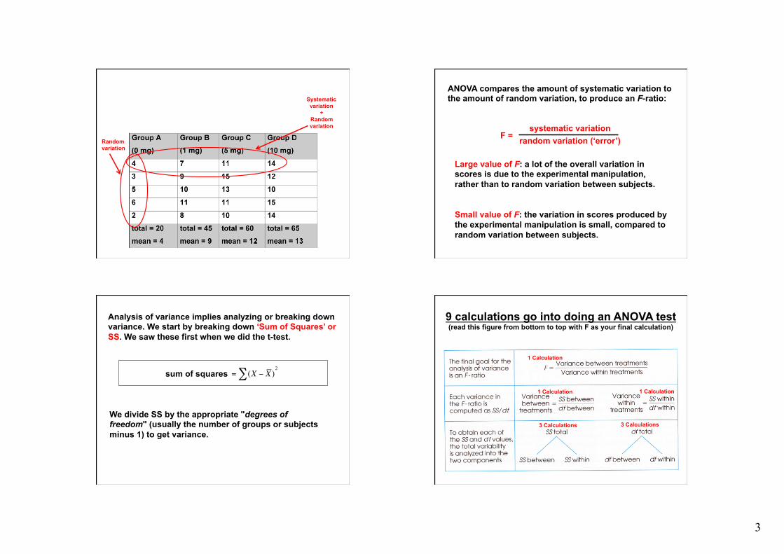
followed by a memory test (words remembered from a list) Variation in the set of scores comes from TWO sources:
• Random variation from the subjects themselves (due to individual variations in motivation, aptitude, mood, ability to understand instructions, etc.).
• Systematic variation produced by the experimental manipulation.
3
Random variation
Systematic variation
+ Random variation
Large value of F: a lot of the overall variation in scores is due to the experimental manipulation, rather than to random variation between subjects.
Small value of F: the variation in scores produced by the experimental manipulation is small, compared to random variation between subjects.
systematic variation random variation (‘error’) F =
ANOVA compares the amount of systematic variation to the amount of random variation, to produce an F-ratio:
Analysis of variance implies analyzing or breaking down variance. We start by breaking down ‘Sum of Squares’ or SS. We saw these first when we did the t-test.
sum of squares
!
= (X " X )#2
We divide SS by the appropriate "degrees of freedom" (usually the number of groups or subjects minus 1) to get variance.
9 calculations go into doing an ANOVA test (read this figure from bottom to top with F as your final calculation)
1 Calculation
3 Calculations
1 Calculation 1 Calculation
3 Calculations

4
step 1 The null hypothesis:
!
H0 :µ1 = µ2 = µ3 = µ4
steps 2, 3 & 4 Calculate 3 SS values:
1) Total 2) Between treatments 3) Within treatments
No treatment effect
set alpha level: α = .05
Total SS
Total SS
!
= (Xi "G )2#
step 2
!
G = 9.5
!
SSTotal = 297
Between treatments SS step 3
SSbetween treatments
!
= n (X 1 "G )2 + (X 2 "G )2 + (X 3 "G )2 + (X 4 "G )2[ ]SSbetween treatments= 245
!
X 1 = 4
!
X 2 = 9
!
X 3 =12
!
X 4 =13n = number of participants
Within treatments SS step 4
!
SS1 = (Xi " X 1)2#
!
SS2 = (Xi " X 2)2#
!
SS3 = (Xi " X 3)2#
!
SS4 = (Xi " X 4 )2#
!
X 1 = 4
!
X 2 = 9
!
X 3 =12
!
X 4 =13
SSwithin treatments= SS1 + SS2 +SS3 +SS4 = 52
5
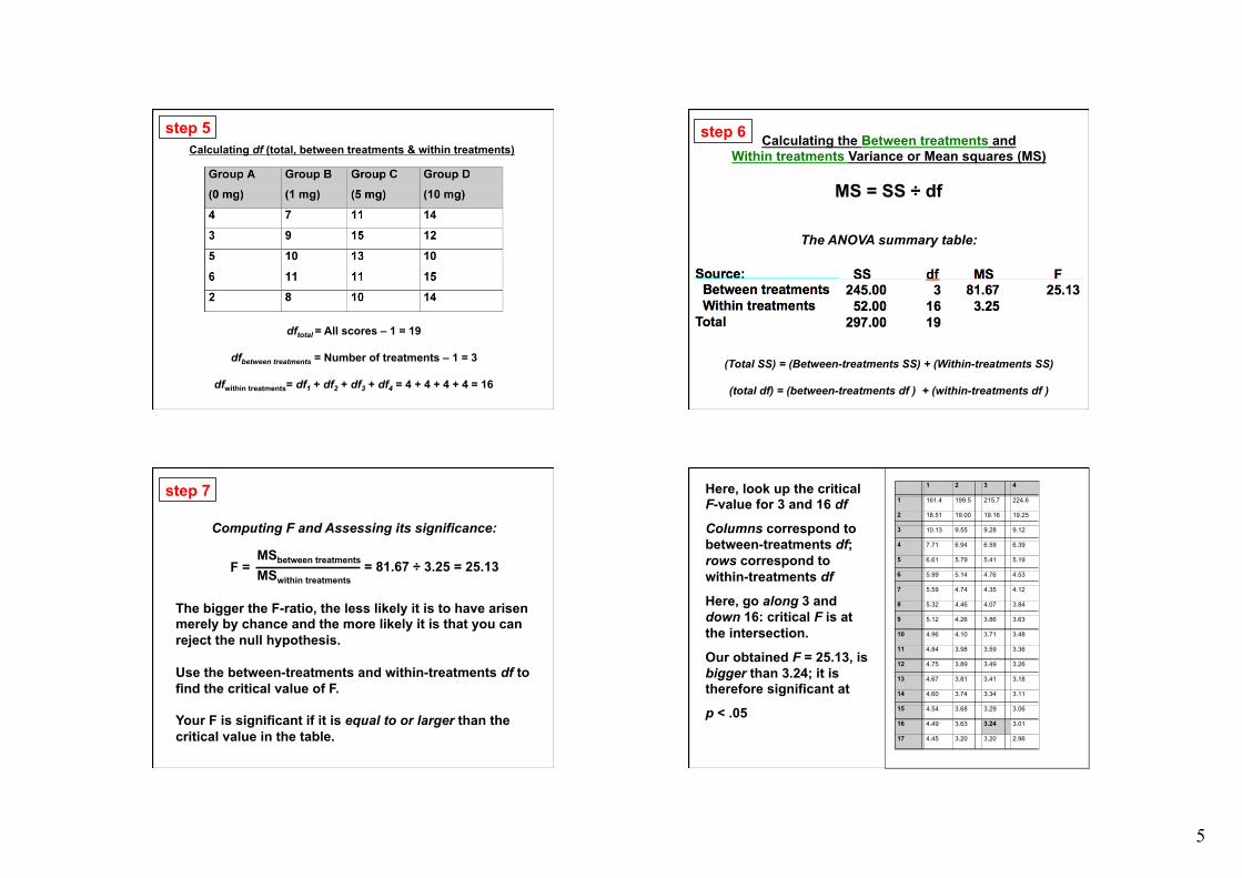
Calculating df (total, between treatments & within treatments)
dftotal = All scores – 1 = 19
dfbetween treatments = Number of treatments – 1 = 3
dfwithin treatments= df1 + df2 + df3 + df4 = 4 + 4 + 4 + 4 = 16
step 5
The ANOVA summary table:
(Total SS) = (Between-treatments SS) + (Within-treatments SS)
(total df) = (between-treatments df ) + (within-treatments df )
step 6 Calculating the Between treatments and Within treatments Variance or Mean squares (MS)
MS = SS ÷ df
Computing F and Assessing its significance: The bigger the F-ratio, the less likely it is to have arisen merely by chance and the more likely it is that you can reject the null hypothesis. Use the between-treatments and within-treatments df to find the critical value of F. Your F is significant if it is equal to or larger than the critical value in the table.
step 7
F = MSbetween treatments
MSwithin treatments = 81.67 ÷ 3.25 = 25.13
1 2 3 4
1 161.4 199.5 215.7 224.6
2 18.51 19.00 19.16 19.25
3 10.13 9.55 9.28 9.12
4 7.71 6.94 6.59 6.39
5 6.61 5.79 5.41 5.19
6 5.99 5.14 4.76 4.53
7 5.59 4.74 4.35 4.12
8 5.32 4.46 4.07 3.84
9 5.12 4.26 3.86 3.63
10 4.96 4.10 3.71 3.48
11 4.84 3.98 3.59 3.36
12 4.75 3.89 3.49 3.26
13 4.67 3.81 3.41 3.18
14 4.60 3.74 3.34 3.11
15 4.54 3.68 3.29 3.06
16 4.49 3.63 3.24 3.01
17 4.45 3.20 3.20 2.96
Here, look up the critical F-value for 3 and 16 df
Columns correspond to between-treatments df; rows correspond to within-treatments df
Here, go along 3 and down 16: critical F is at the intersection.
Our obtained F = 25.13, is bigger than 3.24; it is therefore significant at
p < .05

6
Interpreting the Results: A significant F-ratio merely tells us is that there is a statistically-significant difference between our experimental conditions; it does not say where the difference comes from. In our example, it tells us that caffeine dosage does make a difference to memory performance. BUT the difference may be ONLY between: Caffeine VERSUS No-Caffeine AND there might be NO difference between: Large dose of Caffeine VERSUS Small Dose of Caffeine
To pinpoint the source of the difference we can do: (t – tests)
(a) planned comparisons - comparisons between (two) groups which you decide to make in advance of collecting the data. (b) post hoc tests - comparisons between (two) groups which you decide to make after collecting the data: Many different types - e.g. Newman-Keuls, Scheffé, Bonferroni.
Assumptions underlying ANOVA:
ANOVA is a parametric test (like the t-test)
It assumes:
(a) data are interval or ratio measurements;
(b) conditions show homogeneity of variance;
(c) scores in each condition are roughly normally distributed.
Using SPSS for a one-way independent-measures ANOVA on effects of alcohol on time taken on some task such as whack a mole Three groups (10 individuals in each) Treatments: Group 1: two drinks Group 2: one drink Group 3: no alcohol Dependent variable: Time taken to whack 20 ten moles

7
Data Entry
RUNNING SPSS (Analyze > compare means > One Way ANOVA)

8
Click ‘Options…’ Then Click Boxes: Descriptive; Homogeneity of variance test; Means plot
SPSS output
Trend tests: (Makes sense only when levels of Independent Variable correspond to differing amounts of something - such as caffeine dosage - which can be meaningfully ordered).
Linear trend: Quadratic trend:
(one change in direction)
Cubic trend: (two changes in direction)
With two groups, you can only test for a linear trend. With three groups, you can test for linear and quadratic trends. With four groups, you can test for linear, quadratic and cubic trends.

9
Conclusions:
One-way independent-measures ANOVA enables comparisons between 3 or more groups that represent different levels of one independent variable.
A parametric test, so the data must be interval or ratio scores; be normally distributed; and show homogeneity of variance.
ANOVA avoids increasing the risk of a Type 1 error.