1

Report on

Analysis of the Human Musculoskeletal System and Simulation-Based Design of

Assistive Devices Using OpenSim

Submitted in partial fulfilment of the course ME F376: Design Project

by

Jalaj Maheshwari (2011A4PS224G)

under the supervision of

Prof. D.M. Kulkarni

Associate Professor, Department of Mechanical Engineering

BIRLA INSTITUTE OF TECHNOLOGY AND SCIENCE, PILANI

K.K. BIRLA GOA CAMPUS

3rd May, 2014

2

Acknowledgements

I am very grateful to Prof. D.M. Kulkarni, Associate Professor at the Department of Mechanical

Engineering, for mentoring me and giving me the opportunity to have a great learning

experience while doing this project.

I thank Tanay Choudhary and Karthik P. Sundaram, my team mates, for their contributions

without which this project wouldn’t have come together.

I am also thankful to Dr. Ranjit Patil, instructor-in-charge of the course ME F376: Design Project.

3

Abstract

Biological systems are much more complex than man-made systems. Hence, research in

biomechanics is done in an iterative process of hypothesis and verification, including several

steps of modeling, computer simulation and experimental measurements. This design project

explores the power and relevance of numerical methods employed by state-of-the-art

modeling and simulation tools (OpenSim in this case) in the context of research in biomechanics

of the human musculoskeletal system. It is divided into 3 independent sections – joint reaction

estimation, simulation based design to reduce metabolic cost, and simulation based design to

prevent ankle injury – each with a different type of computational analysis. The applications

and merits of these methods are looked into in addition to acknowledging their limitations and

simplifying assumptions. We realize that, given reliable experimental data, accurate and

insightful results can be arrived at and hypotheses validated, using such methods. They also

circumvent many of the cumbersome, expensive and often invasive experimental methods

required to achieve the same results. Apart from validating hypotheses, these results can be

exploited to a great effect in the rapid, iterative evaluation and optimization of designs of

assistive devices and training programs for rehabilitation, or enhancement of athletic

performance.

4

TABLE OF CONTENTS

1 Introduction ............................................................................................................................ 6

1.1 The Human Musculoskeletal System ............................................................................... 6

1.2 OpenSim ........................................................................................................................... 8

2 Joint Reaction Analysis ............................................................................................................ 9

2.1 Introduction ...................................................................................................................... 9

2.2 Joint Reaction Loads ......................................................................................................... 9

2.3 Static Optimization ......................................................................................................... 11

2.4 Joint Reaction Analysis ................................................................................................... 12

2.5 Joint Reaction Load at the Knee Joint (Methodology) ................................................... 13

2.6 Joint Reaction Analysis in OpenSim ............................................................................... 14

2.7 Simulation in OpenSim ................................................................................................... 15

2.8 Results of Joint Reaction Analysis .................................................................................. 15

2.8.1 Validation of Results ............................................................................................... 15

2.8.2 Force and Moment Plots for a Gait Cycle ............................................................... 17

2.9 Conclusion ...................................................................................................................... 19

3 Simulation-Based Design to Reduce Metabolic Cost ............................................................ 20

3.1 Introduction .................................................................................................................... 20

3.2 OpenSim Simulation ....................................................................................................... 21

3.2.1 Model Properties .................................................................................................... 21

3.2.2 Simulating Unassisted Walking ............................................................................... 22

3.2.3 Metabolics of Unassisted Walking .......................................................................... 25

3.2.4 Building Assistive Devices ....................................................................................... 26

3.2.5 Simulate Walking with Passive Devices .................................................................. 28

3.2.6 Simulate Walking with an Active Device................................................................. 29

3.3 Results ............................................................................................................................ 30

3.4 Conclusion ...................................................................................................................... 34

4 Simulation-Based Design to Prevent Ankle Injuries ............................................................. 35

4.1 Introduction .................................................................................................................... 35

4.2 OpenSim Simulation ....................................................................................................... 36

5

4.2.1 Model Properties .................................................................................................... 36

4.2.2 Simulating Unassisted Landing on Inclined Platform ............................................. 38

4.2.3 Simulating with Passive Ankle Foot Orthosis .......................................................... 39

4.2.4 Simulating with Active Ankle Foot Orthosis ........................................................... 40

4.2.5 Simulating with Muscle Co-activation .................................................................... 41

4.3 Results ............................................................................................................................ 42

4.4 Conclusion ...................................................................................................................... 43

5 Table of Figures ..................................................................................................................... 44

6 References ............................................................................................................................ 45

6

1 INTRODUCTION

1.1 THE HUMAN MUSCULOSKELETAL SYSTEM

The human musculoskeletal system consists of the bones, muscles, ligaments and tendons. The

function of the musculoskeletal system is to:

protect and support the internal structures and organs of the body

allow movement

give shape to the body

produce blood cells

store calcium and phosphorus

produce heat.

This project is concerned primarily with the first and second functions, i.e. support and

movement.

The Skeletal System

The skeletal system is comprised of bones and joints and provides the basic supporting

structure of the body. It consists of the joined framework of bones called the skeleton. The

human skeleton is made up of 206 bones.

Bones

Bone is a dry, dense tissue composed of a calcium-phosphorus mineral and organic matter and

water. Bone is covered with a living membrane called the periosteum. The periosteum contains

bone-forming cells, the osteoblasts.

The centre of bone contains marrow where blood vessels, fat cells and tissue for manufacturing

blood cells are all found.

There are four main shapes of bones:

flat e.g. ribs

irregular e.g. vertebrae

short e.g. hand (carpals)

long e.g. upper arm (humerus)

Joints

A joint is an area where two or more bones are in contact with each other. Joints allow

movement. The bones forming the joint are held together by ligaments.

7

There are 3 types of joints:

1. fibrous or immovable e.g. skull

2. cartilaginous or slightly moveable e.g. vertebrae

3. synovial or freely movable:

a) ball and socket e.g. hip

b) hinge e.g. elbow.

c) gliding e.g. carpals at wrist

d) pivot e.g. radius and ulna

Movement

There are certain terms that are used to describe the movement of bones:

Abduction - movement away from the body

Adduction - movement towards the body

Flexion - bending a limb towards the body

Extension - extending a limb away from the body

Rotation - movement around a central point

The Muscular System

The human body is composed of over 500 muscles working together to facilitate movement.

The major function of the muscular system is to produce movements of the body, to maintain

the position of the body against the force of gravity and to produce movements of structures

inside the body.

Structure

Tendons attach muscle to bone. There are 3 types of muscles:

1. Skeletal (voluntary) muscles are attached to bone by tendons

2. Smooth (involuntary) muscles control the actions of our gut and blood vessels

3. Cardiac muscle in the heart

Movement

Muscles contract (shorten) and relax in response to chemicals and the stimulation of a motor

nerve. Such motion pulls or pushes the bones with them. Muscles usually work in pairs, for

example, the biceps flex the elbow and the triceps extend it.

8

1.2 OPENSIM

Figure 1: OpenSim logo

Models of the musculoskeletal system enable one to study neuromuscular coordination,

analyze athletic performance, and estimate musculoskeletal loads. OpenSim is a state-of-the-

art, freely available, user extensible software system created by the NIH National Center for

Simulation in Rehabilitation Research (NCSRR), that lets users develop models of

musculoskeletal structures and generate dynamic simulations of movement. In OpenSim, a

musculoskeletal model consists of rigid body segments connected by joints. Muscles span these

joints and generate forces and movement. Once a musculoskeletal model is created, OpenSim

enables users to study the effects of musculoskeletal geometry, joint kinematics, and muscle-

tendon properties on the forces and joint moments that the muscles can produce.

The software provides a platform on which the biomechanics community can build a library of

simulations that can be exchanged, tested, analyzed, and improved through multi-institutional

collaboration. The underlying software is written in ANSI C++, and the graphical user interface

(GUI) is written in Java. OpenSim technology makes it possible to develop customized

controllers, analyses, contact models, and muscle models among other things. These plugins

can be shared without the need to alter or compile source code. Users can analyze existing

models and simulations and develop new models and simulations from within the GUI.

The long-term goals of the OpenSim community is to provide high-quality, easy-to-use, bio-

simulation tools that allow for significant advances in rehabilitation and biomechanics research.

9

2 JOINT REACTION ANALYSIS

2.1 INTRODUCTION

When we use our bodies to move and perform tasks, our joint tissues carry loads that affect

joint function and their health. Quantifying these loads is one of the most important and

challenging problems in biomechanics. OpenSim has tools to help us do this.

Individual health and mobility are dependent on the preservation of joint health. There is a

need to understand joint structures and the physical demands on them in order to design

various components such as joint replacements, orthoses etc. It is important to prevent failure

of these components by anticipating the loads they will operate under. Measuring these loads

directly can be difficult and invasive, so an alternative is to use models to represent the

musculoskeletal system and calculate estimates of various joint loads. Using OpenSim, such

calculations can be performed through Joint Reaction Analysis.

2.2 JOINT REACTION LOADS

Joint Reaction Analysis is a method that takes the model, its motion and the forces applied to it,

and then calculates the reaction forces and moments

that result at the joints. These forces and moments

are called joint reaction loads.

The schematic shown on the right side is a 2-D

musculoskeletal representation of the pelvis and

articulating leg. This limb model contains rigid

segments representing bones, joints that let them

articulate, and muscles that can apply forces to move

the model. Ground reaction forces are applied to the

foot and subsequent reaction forces at various joints

are determined.

10

To analyze a specific part of the model such as the

knee-joint loads applied at the tibia (represented in blue), kinematics and muscle forces

obtained from the above model are applied on a small-scale local model to calculate reaction

loads at proximal and distal points.

In this model, the knee joint is an elliptical joint where the tibia rotates and translates around

the femoral condyle. To obtain the load at the tibia plateau, the joint is cut apart to measure

the load across the tibia-femoral joint interface.

Figure 3: Forces on tibia

When the tibia moves in space around the elliptical joint, the muscle forces not only facilitate

this motion but also act to pull the tibia up into the femur. As a result, the femur produces

reaction loads ( ) to prevent the tibia from penetrating this ellipse, thus allowing the tibia to

rotate and translate around the ellipse. These loads that constrain the motion of the tibia in this

manner are called joint reaction loads.

Figure 2: 2-D musculoskeletal representation of the pelvis and articulating leg

11

In order to calculate load estimates for human walking subjects, the following key pieces of

information must first be determined –

1. Model: Describes the geometry, bones, joints and muscles.

2. Kinematics: Describes the walking motion.

3. External Forces: Forces applied by the ground to the feet.

4. Muscle Forces: Forces that actuate the model.

Once known, this data is used to estimate the resulting reaction forces at the joints. However,

only the first three components can be obtained using methods such as gait analysis or other

measurement techniques. The muscle forces cannot be directly measured, and are thus

estimated using various tools provided by OpenSim before joint loads are calculated.

2.3 STATIC OPTIMIZATION

Static Optimization is a technique used to estimate muscle forces prior to the calculation of

joint loads. In Static Optimization, a model is first specified that represents the subject

geometry, after which joint kinematics (represented by green arrows) are provided to describe

the motion of the model. Finally, external loads between the feet and the ground are specified.

As output, Static Optimization chooses one possible distribution of muscle forces that produces

the measured joint kinematics. It also uses a muscle model to measure the activations that

have produced these muscle forces. This gives a complete dynamic description of the system.

12

Figure 4: Joint kinematics required for static optimization

2.4 JOINT REACTION ANALYSIS

Joint Reaction Analysis is a post-processing method that traverses through the model and

calculates reaction forces and moments in all the joints. It starts with the most distal segment

of each limb (the foot). All external forces and muscle forces are used to calculate the resultant

load ( at the proximal joint (the ankle).

13

Figure 5: Joint reaction analysis

The next step involves moving up the limb and applying the equal and opposite ankle load on

the tibia, along with all other known forces to calculate the reaction forces ( at the

proximal knee joint.

This method can be extended to calculate reaction forces in a similar manner for the pelvis as

well using the previously calculated reaction load at a distal joint (tibia) to determine the

reaction load at the proximal joint.

2.5 JOINT REACTION LOAD AT THE KNEE JOINT (METHODOLOGY)

In this calculation, Joint Reaction Analysis isolates the body distal to the joint of interest; i.e. the

tibia. This method then constructs the 6-D Newton-Euler equation of motion, which defines the

kinematics for the tibia in space. This equation combines the translational and rotational

dynamics of a rigid body, thus providing an expression for the linear and rotational acceleration

of the tibia about its center of mass ( .

The 5 forces that act on the body (tibia) are:

External forces ( ); i.e. gravity forces (

Muscle forces ( ) as estimated by Static Optimization techniques

14

Distal Reaction load ( ) at the ankle

Proximal Reaction load ( ) at the knee joint (to be determined)

Constraint forces ( ) if specified

Figure 6: Free body diagram of the tibia

These forces are equal to the inertial forces for the body, and hence we get:

∑ ∑

Now, we solve for the reaction load at the knee joint ( ) as:

(∑ ∑ )

2.6 JOINT REACTION ANALYSIS IN OPENSIM

Model used: subject01_simbody_adjusted.osim which is a modified version of

gait2392_simbody.osim. This is a gait model with torso, pelvis and both legs. The model has 23

degrees of freedom and 92 muscles. The upper extremity has been simplified by lumping

together the torso, arms and head to represent the trunk as a whole.

15

Time Range: 0.5-2 seconds of the gait cycle

External load: Ground reaction forces from force plate measurements.

Muscle forces obtained from static optimization performed in OpenSim are stored in a separate

file, and are subsequently fed as input for the calculation of joint reaction loads.

2.7 SIMULATION IN OPENSIM The model is loaded by going to File -> Open Model and selecting

subject01_simbody_adjusted.osim

We then go to Tools -> Analyze -> Settings -> Load Settings and selecting

setup_static_optimization.xml. This file loads the ground reaction forces from

foot_floor_loads.xml as well as the kinematics file subject01_walk1_Kinematics.sto for

the motion of the model.

When we click Run in the Analyze window, OpenSim simulates the motion to determine

the muscle actuator forces and writes them to the directory ResultsStaticOptimization.

We then load setup_JointReaction in a similar manner and run it from the Analyze

window. This simulation uses muscle forces determined in the above step stored in the

ResultsStaticOptimization directory as input to determine the required joint reaction

forces.

The forces and moments can be visualized graphically by going to Tools -> Plot and loading the

subject01_JointReaction_ReactionLoads.sto file for the Y coordinates. We then choose the

required forces and moments and plot them against time.

2.8 RESULTS OF JOINT REACTION ANALYSIS

2.8.1 Validation of Results The model is a tree-structure originating from the pelvis, which is free to move in space. Hence,

the ground-pelvis joint is free to rotate and translate without any constraint, and should

experience no reaction load. In order to validate the results obtained from Joint Reaction

Analysis in OpenSim, we first ensured that the net reaction load between the ground and pelvis

is zero. The following graph obtained using the Plot tool of OpenSim illustrates the same:

16

Figure 7: Net reaction load between the ground and pelvis is zero

Another method to validate the obtained results is to ensure that the moment components of

reaction loads at the hip are zero. This is because the hip joint is a ball-and-socket joint, where

the femoral head is a ball rotating within the socket of the pelvis. Such an arrangement allows

the femur to rotate freely while restricting translation so that the ball of the femur does not

penetrate the socket of the pelvis. Since there is no restriction on rotational motion, moment

components at the hip must be zero. The following graph illustrates this:

Figure 8: Moment components at the hip are zero

Thus, the results obtained from Joint Reaction Analysis can be accepted as the above 2 cases

have shown the expected results.

17

2.8.2 Force and Moment Plots for a Gait Cycle

Figure 9: Forces acting between the ankle and talus of the right foot

Figure 10: Moments acting between the ankle and talus of the right foot

18

Figure 11: Forces acting between the knee and tibia of the right leg

Figure 12: Moments acting between the knee and tibia of the right leg

The major spikes in force and moment in the X and Y directions at the knee joint and ankle joint

are seen at 0.75 seconds and 1.25 seconds respectively in the gait cycle correspond to the pre-

swing and terminal swing stages of limb advancement respectively as shown below:

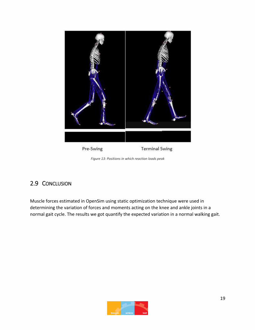
19

Figure 13: Positions in which reaction loads peak

2.9 CONCLUSION

Muscle forces estimated in OpenSim using static optimization technique were used in

determining the variation of forces and moments acting on the knee and ankle joints in a

normal gait cycle. The results we got quantify the expected variation in a normal walking gait.

20

3 SIMULATION-BASED DESIGN TO REDUCE METABOLIC COST

3.1 INTRODUCTION

The metabolic and mechanical requirements of walking are considered to be of fundamental

importance to the health, physiological function and even the evolution of modern humans.

Energy minimization is widely considered a primary goal of the central nervous system [1]. The

rate at which a human expends metabolic energy while walking (gross metabolic rate) increases

with increasing speed. However, humans also require a continuous basal metabolic rate to

maintain normal function. The energetic cost of walking itself is therefore best understood by

subtracting basal metabolic rate from gross metabolic rate, yielding net metabolic rate. These

measures of walking energetics are based on how much oxygen people consume per unit time.

Walking is described and characterized in the context of the gait cycle (figure 14), with the start

of the cycle traditionally coinciding with the heel striking the ground. In walking, the foot is on

the ground for a little more than 60% of the gait cycle. This interval is referred to as the stance

phase. The stance phase begins and ends with both feet on the ground, which are known as

periods of double-limb support. The intervening time, when only one limb is on the ground, is

known as single-limb support. During the remainder of the gait cycle (i.e. slightly less than 40%),

the foot is off the ground as the limb is swung forward to begin the next stride. This interval is

referred to as the swing phase.

Figure 14: Gait Cycle

21

Enhancing our understanding of the relative costs of the various phases of the bipedal gait cycle

has implications both on the development of general theories of locomotion, and on more

practical issues, such as treating gait disorders or designing lower limb prostheses.

Using a model of muscle energy expenditure [2], it is possible to derive estimates of the

metabolic cost incurred by the muscles during each phase of the gait cycle.

3.2 OPENSIM SIMULATION

We use OpenSim's Computed Muscle Control (CMC) Tool to generate muscle-driven

simulations of a typical, unloaded gait on a simplified model of the musculoskeletal system,

with the aim of designing and evaluating devices to assist locomotion. The subject considered in

this simulation is a 75kg, 1.8m tall male, walking at 1.2 m/s on a treadmill.

3.2.1 Model Properties The model used is ‘gait10dof18musc’, which consists of trunk, pelvis and leg segments with 10

degrees of freedom and 18 muscles. It has the following simplifications:

The upper extremity has been lumped into one torso segment to represent the trunk,

arms, and head.

The model includes only one degree of freedom at each hip and ankle and between the

torso segment and pelvis.

The number of muscles in the model has been reduced by lumping the key

flexor/extensor muscles in the lower extremities.

To further simplify the simulation to focus on muscle-driven simulation and metabolic cost, we

used a modified version of the model that has already been scaled and run through the

Residual Reduction Algorithm. In particular:

The generic model has been scaled to match the subject's anthropometry (i.e., mass and

segment lengths) using the Scale Tool.

The Inverse Kinematics Tool was used to determine the model coordinates, as functions

of time, which yield the observed marker trajectories.

The Residual Reduction Algorithm (RRA) Tool used the scaled model and the inverse

kinematics results to make small adjustments to segment inertial properties and the

joint kinematics for the trial to achieve a model and kinematics that are dynamically

consistent with the measured ground reaction forces (available from experiments). The

purpose of residual reduction is to minimize the effects of modeling and marker data

22

processing errors that aggregate and lead to large nonphysical compensatory forces

called residuals.

Figure 15: A comparison of the modified model (L) and the generic model (R)

3.2.2 Simulating Unassisted Walking Beginning with the kinematics data that are output by the RRA Tool, the CMC algorithm finds a

set of muscle excitations that track the input kinematics (within an error tolerance). CMC solves

the muscle redundancy problem by minimizing the sum of squared muscle activations.

3.2.2.1 Loading and exploring the motion

1. We loaded the RRA adjusted kinematics file by selecting File>Load Motion... and

navigating to gait10dof18musc\RRA\ResultsRRA, then selecting

subject_adjusted_Kinematics_q.sto.

2. We visualized the ground reaction forces (GRFs) for the motion, by associating the

following motion data with the current one -

gait10dof18musc\ExperimentalData\subject01_walk_grf.mot. Now when we played the

motion, a green arrow corresponding to the experimentally-measured ground reaction

force vector was seen.

23

Figure 16: Ground reaction force vectors from experimental data incorporated into the motion

3. By examining the motion, we determined the times of key gait cycle events. The time

range between consecutive heel strikes of the same (right) foot was found to be from

0.6 to 1.9 seconds. This defines a gait cycle for this trial.

3.2.2.2 Using CMC to generate a muscle-driven simulation

1. The CMC Tool was launched from Tools>Computed Muscle Control. It operates on the

model currently selected in the GUI (walk_subject01 in our case).

2. We loaded pre-configured CMC settings from the file CMC\walk_Setup_CMC.xml. It uses

the RRA adjusted kinematics we loaded in the previous section. There was no need to

filter kinematics; the data was already smooth since it resulted from a run of RRA.

3. The Tracking tasks file used, gait10dof_Kinematics_Tracking_Tasks.xml, defines the

coordinates that OpenSim should track (in our case, all coordinates in the model).

4. We specified the time range we found earlier that corresponds to one gait cycle (0.6 to

1.9 seconds).

5. We specified the external loads (ground reaction forces) as well as appended reserve

actuators (forces/torques that are added about each joint and at the pelvis to augment

the muscle force when needed in order to enable the simulation to run) in the Actuators

and External Loads tab from the file gait10dof_Reserve_Actuators.xml.

6. Finally, we ran the CMC Tool and saw the model animate as results were generated.

3.2.2.3 Evaluating the simulation results

1. We played the results using the Motion Slider Panel, and observed the muscles changing

colour from blue to red as activation increased.

24

Figure 17: Visualizing the CMC results

2. We plotted the kinematic tracking errors to make sure the kinematics from the CMC

simulation are a good match with the input kinematics. It shows the difference between

the RRA and CMC curves. These errors should generally be 2 degrees or less for gait

simulations, as indicated by the plotted thresholds.

Figure 18: The kinematic tracking errors are within the tolerable range

3. We then looked at the muscle forces from the simulation for muscles that cross the

ankle joint (gastrocnemius, soleus and tibialis anterior muscles on the right leg), by

25

plotting the walk_subject_Actuation_force.sto file from the CMC results folder against

the gait cycle time.

Figure 19: Muscle forces (N) computed for unassisted walking

3.2.3 Metabolics of Unassisted Walking The metabolics calculators in OpenSim can calculate the rate or total amount of energy

consumption for each muscle in the model, and for the whole body. The models of metabolics

from Umberger et al. (2003) and (2010) account for the effect of muscle mass, the ratio of fast-

and slow-twitch fibers (anaerobic and aerobic muscle fiber types), and the

lengthening/shortening velocity. The model we worked with includes a set of metabolic probes

to calculate the energy consumed by all the muscles in the model, as well as each individual

muscle on its own. The aerobic scale factor used in the probes is 1.5, which corresponds to

primarily aerobic conditions. This is a reasonable assumption for calculating the metabolic rate

while walking, since it doesn’t involve anaerobic conditions.

By plotting the metabolics_TOTAL from the walk_subject_MetabolicsReporter_probes.sto file in

the CMC results folder against time, we can generate a graph of the total instantaneous

metabolic energy consumed by all muscles (in units of Watts) over the walking trial. The total

rate of metabolic energy consumption is found to be highest just before the left and right foot

toe-offs. This is expected since maximum contraction of the relevant muscles is required for

lifting each foot.

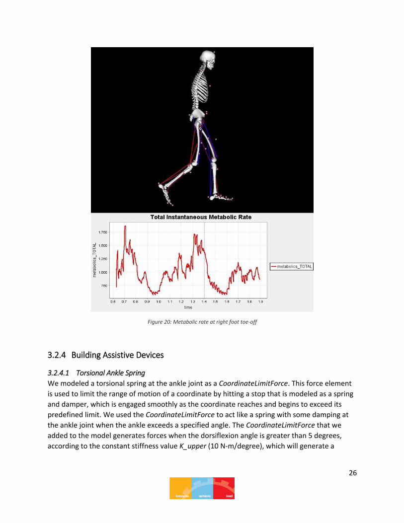
26

Figure 20: Metabolic rate at right foot toe-off

3.2.4 Building Assistive Devices

3.2.4.1 Torsional Ankle Spring

We modeled a torsional spring at the ankle joint as a CoordinateLimitForce. This force element

is used to limit the range of motion of a coordinate by hitting a stop that is modeled as a spring

and damper, which is engaged smoothly as the coordinate reaches and begins to exceed its

predefined limit. We used the CoordinateLimitForce to act like a spring with some damping at

the ankle joint when the ankle exceeds a specified angle. The CoordinateLimitForce that we

added to the model generates forces when the dorsiflexion angle is greater than 5 degrees,

according to the constant stiffness value K_upper (10 N-m/degree), which will generate a

27

plantar flexion moment. Note that the transition property determines the region in which the

stiffness transitions from zero (before the limit) to K beyond the limit.

We entered the commands below in the ScriptingShell window to create a new model and add

a torsional spring to this model:

# Get a handle to the current model and create a new copy baseModel = getCurrentModel() ankleSpringModel = baseModel.clone() ankleSpringModel.setName(baseModel.getName() + '_ankle_spring') # Create the spring we'll add to the model (a CoordinateLimitForce in

OpenSim) ankleSpring = modeling.CoordinateLimitForce() ankleSpring.setName('AnkleLimitSpringDamper') # Set the coordinate for the spring ankleSpring.set_coordinate('ankle_angle_r') # Add the spring to the model ankleSpringModel.addForce(ankleSpring) # Load the model in the GUI loadModel(ankleSpringModel)

Using the Property Editor in the GUI, we set the parameters for the spring as follows:

upper_stiffness = 10.0 → This is the stiffness of the ankle spring device during ankle

dorsiflexion.

upper_limit = 5.0 → The spring is "engaged" when the ankle dorsiflexion angle is greater

than 5 degrees.

lower_stiffness = 1.0 → The CoordinateLimitForce will also generate forces preventing

excess plantarflexion, as specified by the lower_stiffness and lower_limit values.

lower_limit = -90.0 → Allow the full range of plantarflexion motion.

damping = 0.01 → A small damping term.

transition = 2.0 → This term dictates the transition from zero to constant stiffness as the

coordinate exceeds its limit (upper or lower), in degrees.

3.2.4.2 Bi-articular path spring

We also created a model with a passive spring that acts along a path between the femur and

foot segments. The path spring element takes a GeometryPath (similar to muscles), along with

resting length, stiffness, and dissipation values. We used the spring to augment the

gastrocnemius muscle (primary calf muscle) with a stiffness of 10000 N-m.

The following commands were used to create this model:

# Get a handle to the current model and create a new copy baseModel = getCurrentModel()

28

pathSpringModel = baseModel.clone() pathSpringModel.setName(baseModel.getName() + '_path_spring') # Create the spring we'll add to the model (a PathSpring in OpenSim) pathSpring = modeling.PathSpring() pathSpring.setName('BiarticularSpringDamper') # Set geometry path for the path spring to match the gastrocnemius muscle gastroc = pathSpringModel.getMuscles().get('gastroc_r') pathSpring.set_GeometryPath(gastroc.getGeometryPath()) # Add the spring to the model pathSpringModel.addForce(pathSpring) # Load the model in the GUI loadModel(pathSpringModel)

Its parameters were set as:

resting_length = 0.4

stiffness = 10000.0

dissipation = 0.01 → The dissipation factor (s/m) of the PathSpring.

Figure 21: The bi-articular path spring visualized in green in the new model

3.2.5 Simulate Walking with Passive Devices A similar procedure as described earlier for unassisted walking simulation was used, but with

the new ankle spring and path spring incorporated models we created.

29

3.2.6 Simulate Walking with an Active Device We also used the predefined model subject01_metabolics_path_actuator.osim which has an

active bi-articular path actuator (PlantarFlexAssist), to study its effect on the metabolic cost.

The geometry path of the actuator is the same as the passive path spring we created, but the

tension in this actuator is governed by a user-defined control signal over the time course of the

gait simulation. The optimal_force property of the actuator scales the input control signal (i.e. if

the input control signal is 1 and the optimal force value is 10, the tension in the actuator will be

10 N).

The simulation procedure is same as before, with the only difference being in the CMC Tool

step. This time we also added an actuator constraints file, controls.xml which contains the

desired control signal for the path actuator. We used the Excitation Editor to define the signal

as follows:

Figure 22: Desired control signal for path actuator, in the Excitation Editor window

Such a control signal was chosen because the purpose of the path actuator is to reduce the

metabolic cost of walking for the right leg (on which it is mounted), which peaks before the

right foot’s toe off. Hence, that is when maximum assistance is useful. Of course, different

patterns can be tested to arrive at the optimal design iteratively.

30

3.3 RESULTS

The plots below compare the metabolic cost of walking for the different simulations performed.

(Results_CMC corresponds to unassisted walking)

Figure 23: The right Gastrocnemius muscle and its metabolic rate

31

Figure 24: The right Soleus muscle and its metabolic rate

32

Figure 25: The right Iliopsoas muscle and its metabolic rate

33

Figure 26: The right Tibialis Anterior muscle and its metabolic rate

34

Figure 27: Total instantaneous metabolic rate over the gait period

3.4 CONCLUSION

As we can see, different devices decrease the energy cost of gait at different parts of the gait

cycle. Depending on the specific requirements or muscle conditions of the patient, any one of

the assistive devices could be more beneficial to him/her than the others. But in simple terms

overall, the passive ankle spring assistive device gives the most energy efficient gait according

to our simulations.

35

4 SIMULATION-BASED DESIGN TO PREVENT ANKLE INJURIES

4.1 INTRODUCTION

Ankle sprains are one of the most common injuries among people, especially athletes. Ankle

inversion is an injury where the lateral side of the foot is affected. In this type of injury, the

ligaments that restrain ankle inversion (the anterior talo-fibular and calcaneo-fibular ligaments)

are damaged. When the ankle inversion angle exceeds 25ᵒ, it results in an injury and causes a

lot of pain and inflammation [3, 4]. By using OpenSim, we can study the effect of an ankle-foot

orthosis (AFO) by simulating a jump at an angle and evaluate the risk of injury during landing,

and design assistive devices to prevent such injuries.

Figure 28: Tearing of ligaments that restrain ankle inversion

36

4.2 OPENSIM SIMULATION

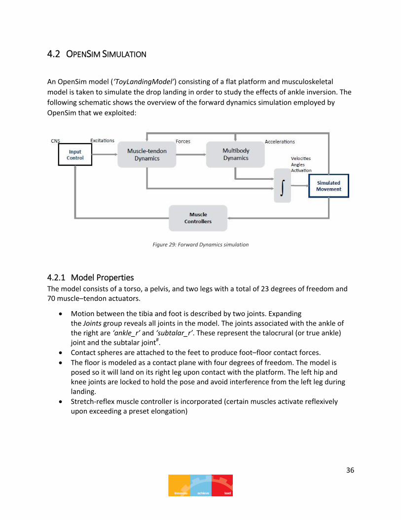
An OpenSim model (‘ToyLandingModel’) consisting of a flat platform and musculoskeletal

model is taken to simulate the drop landing in order to study the effects of ankle inversion. The

following schematic shows the overview of the forward dynamics simulation employed by

OpenSim that we exploited:

Figure 29: Forward Dynamics simulation

4.2.1 Model Properties The model consists of a torso, a pelvis, and two legs with a total of 23 degrees of freedom and 70 muscle–tendon actuators.

Motion between the tibia and foot is described by two joints. Expanding the Joints group reveals all joints in the model. The joints associated with the ankle of the right are ‘ankle_r’ and ‘subtalar_r’. These represent the talocrural (or true ankle) joint and the subtalar joint#.

Contact spheres are attached to the feet to produce foot–floor contact forces.

The floor is modeled as a contact plane with four degrees of freedom. The model is posed so it will land on its right leg upon contact with the platform. The left hip and knee joints are locked to hold the pose and avoid interference from the left leg during landing.

Stretch-reflex muscle controller is incorporated (certain muscles activate reflexively upon exceeding a preset elongation)

37

Figure 30: The musculoskeletal model with platform

# The subtalar joint is a joint of the rear foot and is also known as the talocalcaneal joint. It

occurs at the meeting point of the talus and the calcaneus. The angle between these two bones

is called the subtalar angle. This angle determines the degree of inversion or eversion of the

ankle.

Figure 31: The subtalar joint

38

Later we also added an ankle foot orthosis (AFO) to the model. It is a brace that encumbers the

ankle and foot. It is externally applied and intended to control position and motion of the ankle,

or compensate for weakness.

4.2.2 Simulating Unassisted Landing on Inclined Platform To simulate a drop landing, the following steps were taken:

1. The platform angles were set – platform_rx set to 20ᵒ, platform_ry to 0ᵒ, platform_rz to

0ᵒ, and platform_ty to -0.5 meters. All four platform coordinates were locked. This

prevents the platform from falling or rotating on impact.

2. Certain degrees of freedom (such as the metatarsal plantar flexion) are locked to

simplify the simulation for our particular application.

3. Using the Simulate tool of OpenSim, forward dynamics simulation is performed for a

time period of 0.4 seconds.

4. OpenSim uses the current pose of the model in the GUI as the starting state for the

simulation.

5. The results were then saved as ‘Unassisted’.

On simulating the unassisted motion, we found that on landing, the right subtalar angle reaches

as high as 56.008ᵒ which exceeds the limit for ankle inversion prevention (25ᵒ) by a large value.

The position of foot just before the impact on the floor and at the maximum subtalar angle is

given below:

Figure 32: Position of the foot just before (L) and after (R) landing

39

Since the subtalar angle is more than the limit, the ligaments will be damaged and will result in

ankle inversion injury. This can be avoided by designing an ankle-foot orthosis which limits the

subtalar angle to 25ᵒ.

4.2.3 Simulating with Passive Ankle Foot Orthosis The drop landing simulation was repeated using the model ‘ToyLandingModel_AFO’ which has

the following specifications:

The model has a two-segment passive ankle foot orthosis (AFO).

The AFO has a footplate that is rigidly attached to the foot and a cuff that is rigidly

attached to the tibia.

The footplate and cuff are connected at two hinge points by six dimensional springs,

called bushings#. The bushings resist the relative translation and rotation of the

footplate and cuff.

Figure 33: Ankle Foot Orthosis

# Bushings are independent plain bearings that are inserted into a housing type structure to

provide a bearing surface for rotary applications. Most commonly used bushings are solid, split

and clenched bushings.

40

The simulation procedure is same as before. But before that, we set the translational stiffness

of the medial bushing (which prevents the AFO cuff from translating with respect to the

footplate on the medial side of the brace) to 10,000 in each of the axis directions, in order to

simulate a soft AFO. Then we simulate again with the 10 times the stiffness, i.e., 100,000.

The peak subtalar angles this time were less than before (45ᵒ for soft AFO and 25ᵒ for stiff AFO),

but still not low enough to be mitigate inversion injuries.

4.2.4 Simulating with Active Ankle Foot Orthosis Nowadays, rehabilitation robotics is providing new active devices to help train and optimize

movement. Orthotics for ankle injury prevention has traditionally consisted of passive devices,

but it is possible to create an active mode for landing. By adding a torque motor at the ankle, an

active orthosis model can be created. Optimizing the timing and activation level of the active

orthosis is required to prevent ankle inversion injury.

Using OpenSim, we simulated the landing under an active orthosis (incorporated in the model

‘ToyLandingModel_activeAFO’). Before performing the simulation like before, we needed to

adjust the timing and the activation level of the active orthosis in a way such that the ankle

inversion angle is limited to 25ᵒ while keeping the power and cost requirements minimum. This

is done using the Excitation Editor in the Forward Dynamics tool in OpenSim as below:

Figure 34: Control signal for active orthosis in Excitation Editor

41

The torque profile is edited as shown to activate the orthosis just before landing (which can be

detected by sensors such as accelerometer or angle/force sensors). This way we ensure that the

power source for the orthosis lasts longer.

4.2.5 Simulating with Muscle Co-activation Individuals can modulate the stiffness of the ankle by co-activating muscles in anticipation of

landing. Thus, co-contraction of muscles, especially the inverter and everter muscles, might

reduce ankle inversion during landing. The model we used was equipped with two controllers

that set the level of excitation (control) of the inverter and everter muscles. These controllers

were initially disabled in the model. By enabling them we can explore the effect of increased

muscle co-activity on ankle inversion during the drop-landing. The co-activation controllers

operate in addition to the reflex controllers in the model. The reflex controllers, which were

enabled in the previous simulations (with a gain of 0.85), activate based on the stretch of the

whole muscle–tendon unit. The level of excitation of the muscle is proportional (via a gain) to

the rate that the whole muscle actuator is lengthening.

We ran the forward simulation again on the original unassisted model but with the R-inverter

and R-everter pre-activation controllers enabled. These controllers activate the specified

muscles (ext_hal_r, flex_dig_r, flex_hal_r, tib_ant_r, tib_post_r for R-inverter and ext_dig_r,

per_brev_r, per_long_r, per_tert_r for R-everter) at a prescribed constant value (0.1 for R-

inverter and 0.3 for R-everter) throughout the simulation.

Figure 35: Inverter muscles' activation before and after co-activation

42

This co-activation did reduce the subtalar angle in unassisted drop, but not enough. It needs to

be used in combination with an AFO in order to be truly effective as an ankle inversion

prevention strategy. Hence, a few more iterations of simulation were performed on

combinations of soft and medium stiffness AFO with low and high co-activation. The soft AFO

and low co-activation correspond to the values already employed in previous independent

simulations. In medium stiffness AFO, the translation stiffness of the passive AFO was changed

to 50,000 and in high co-activation, the inverters’ constant was increased to 0.4 and everters’

to 0.8.

4.3 RESULTS

Figure 36: Inversion angle for different configurations the drop landing was simulated in

As can be seen from the comparison plot above, the subtalar angle was within the acceptable

range only for the active AFO, when each strategy was considered individually.

43

Figure 37: Better design by using a combination of strategies

From the plot above, we found that combining the medium stiffness AFO with high co-

activation produced the most optimum results.

4.4 CONCLUSION

We observed that a variety of configurations of stiffness values, torque profiles and muscle co-

activations are possible. The challenge is to optimize the design keeping in mind the following

costs:

Increasing the AFO's stiffness will increase manufacturing costs and decrease comfort

and performance versatility.

Training programs to increase muscle strength, improve co-activation strategy, improve

landing position, etc. will also have costs.

The amount of time an AFO is active and its maximum torque must be minimized in the

torque profile, since these increase the cost of an already expensive active AFO

exponentially.

On the basis of the above design parameters and the results we got from simulating with their

different combinations, we arrive at the conclusion that a medium stiffness passive AFO

coupled with a training program to achieve high muscle co-activation before landing is the

optimal strategy to be employed in order to prevent ankle inversion injuries.

44

5 TABLE OF FIGURES

Figure 1: OpenSim logo ................................................................................................................... 8

Figure 2: 2-D musculoskeletal representation of the pelvis and articulating leg ......................... 10

Figure 3: Forces on tibia ................................................................................................................ 10

Figure 4: Joint kinematics required for static optimization .......................................................... 12

Figure 5: Joint reaction analysis .................................................................................................... 13

Figure 6: Free body diagram of the tibia ...................................................................................... 14

Figure 7: Net reaction load between the ground and pelvis is zero ............................................ 16

Figure 8: Moment components at the hip are zero ..................................................................... 16

Figure 9: Forces acting between the ankle and talus of the right foot ........................................ 17

Figure 10: Moments acting between the ankle and talus of the right foot ................................. 17

Figure 11: Forces acting between the knee and tibia of the right leg .......................................... 18

Figure 12: Moments acting between the knee and tibia of the right leg ..................................... 18

Figure 13: Positions in which reaction loads peak ........................................................................ 19

Figure 14: Gait Cycle ..................................................................................................................... 20

Figure 15: A comparison of the modified model (L) and the generic model (R) .......................... 22

Figure 16: Ground reaction force vectors from experimental data incorporated into the motion

....................................................................................................................................................... 23

Figure 17: Visualizing the CMC results .......................................................................................... 24

Figure 18: The kinematic tracking errors are within the tolerable range .................................... 24

Figure 19: Muscle forces (N) computed for unassisted walking .................................................. 25

Figure 20: Metabolic rate at right foot toe-off ............................................................................. 26

Figure 21: The bi-articular path spring visualized in green in the new model ............................. 28

Figure 22: Desired control signal for path actuator, in the Excitation Editor window ................. 29

Figure 23: The right Gastrocnemius muscle and its metabolic rate ............................................. 30

Figure 24: The right Soleus muscle and its metabolic rate ........................................................... 31

Figure 25: The right Iliopsoas muscle and its metabolic rate ....................................................... 32

Figure 26: The right Tibialis Anterior muscle and its metabolic rate ............................................ 33

Figure 27: Total instantaneous metabolic rate over the gait period ............................................ 34

Figure 28: Tearing of ligaments that restrain ankle inversion ...................................................... 35

Figure 29: Forward Dynamics simulation ..................................................................................... 36

Figure 30: The musculoskeletal model with platform .................................................................. 37

Figure 31: The subtalar joint ......................................................................................................... 37

Figure 32: Position of the foot just before (L) and after (R) landing ............................................ 38

Figure 33: Ankle Foot Orthosis ..................................................................................................... 39

Figure 34: Control signal for active orthosis in Excitation Editor ................................................. 40

Figure 35: Inverter muscles' activation before and after co-activation ....................................... 41

Figure 36: Inversion angle for different configurations the drop landing was simulated in ........ 42

Figure 37: Better design by using a combination of strategies .................................................... 43

45

6 REFERENCES

[1] Alexander, McNeill R. (2002). "Energetics and optimization of human walking and running:

The 2000 Raymond Pearl memorial lecture" (PDF). American Journal of Human Biology 14 (5):

641–648.

[2] Umberger, B.R., Gerritsen, K.G.M., Martin, P.E. (2003) A model of human muscle energy

expenditure. Computer Methods in Biomechanics and Biomedical Engineering, 6(2):99–111.

[3] Siegler, S., Chen, J., Schneck, C.D. (1990). The effect of damage to the lateral collateral

ligaments on the mechanical characteristics of the ankle joint—an in-vitro study. Journal of

Biomechanical Engineering, 112(2):129–137.

[4] Lapointe, S.J., Siegler, S., Hillstrom, H., Nobilini, R.R., Mlodzienski, A., Techner, L. (1997).

Changes in the flexibility characteristics of the ankle complex due to damage to the lateral

collateral ligaments: an in vitro and in vivo study. Journal of Orthopaedic Research, 15(3):331–

341.

[5] Lamb S.E., Nakash R.A., Withers E.J., Clark M., Marsh J.L., Wilson S. Clinical and cost

effectiveness of mechanical support for severe ankle sprains: design of a randomized controlled

trial in the emergency department. BMC Musculoskelet Disord. 2005; 6(1):61.

[6] Donatelli R.A. 2nd Ed. F.A. Davis; Philadelphia: 1996. The biomechanics of the foot and ankle.

[7] Hertel J., Denegar C., Monroe M.M., Stokes W.L. Talocrural and subtalar joint instability

after lateral ankle sprain. Med Sci Sports. 1999;31(11):1501–1508.