analysis of the chatter instability in a nonlinear model

Analysis of the Chatter Instability

in a Nonlinear Model for Drilling

Sue Ann Campbell

Department of Applied Mathematics,

University of Waterloo, Waterloo, ON N2L 3G1 Canada

Emily Stone

Department of Mathematical Sciences,

The University of Montana, Missoula, MT 59812 U.S.A.

Abstract

In this paper we present stability analysis of a nonlinear model for chatter vibration in a

drilling operation. The results build our previous work [1, 2], where the model was developed

and the nonlinear stability of the vibration modes as cutting width is varied was presented. Here

we analyze the effect of varying cutting depth. We show that qualitatively different stability

lobes are produced in this case. We analyze the criticality of the Hopf bifurcation associated

with loss of stability and show that changes in criticality can occur along the stability boundary,

resulting in extra periodic solutions.

Keywords: delay differential equations, chatter, drilling, centre manifold reduction

1

INTRODUCTION

INTRODUCTION

In a metal cutting operation such as turning, a cutting tool is directed perpendicularly

to the cylindrical workpiece that is spinning along its longitudinal axis (the spindle),

shaving a thin piece of material (a chip) as the spindle turns. Milling involves a similar

local geometry, though multiple teeth in a cogged cutting tool shave a chip off a stationary

work piece as they revolve. Drilling is more difficult to describe owing to the complex

geometry of the drill bit, but at the bottom of the drill the cutting edges also revolve

in the hole and remove a thin chip of material as they go. The twisted grooves in

the side of the drill bit are there to direct the cut chip up and out of the hole being

drilled. Understanding metal cutting and predicting optimal operating conditions has

been a preoccupation of industrial engineers for the past 100 years, and lately high-

speed machining and machining composites have renewed interest in the science of metal

removal. In the aircraft industry drilling holes and filling them comprises a large part of

the effort in manufacturing aircraft, so any gains in drilling technology are subsequently

amplified.

Chatter in metal cutting is a vibration that is initiated by imperfections in the material

being cut, and is maintained by the periodic driving force created from the oscillating

thickness of the chip. Typically the cutting process is modeled as a spring-mass system,

with the stipulation that the cutting force varies with chip thickness, and hence depends

not only on the position of the cutting tool at a given time, but the position of the tool

at the previous revolution of the workpiece. This leads to a delay term in the applied

force on the oscillator, and chatter in metal cutting operations has been successfully

described and predicted by delay differential equations. Tlusty and Tobias were the

original pioneers of this work [3], see also studies by Stepan, Altintas, Bayly [4–8].

In this paper we investigate the chatter instability in a model of metal cutting relevant

to drilling operations. In a previous paper [1] the derivation of the model is presented

along with linear stability calculations for the onset of chatter. In another paper [2]

we document the nonlinear stability of chatter in this model, using approximate center

manifold techniques [9–12]. In both instances the instability parameter is proportional

to the width of cut, the chatter commences as the cutting width is increased past a

critical value, sometimes below the linear stability value, if the bifurcation is subcritical.

Here we extend this study to include the effect of varying the cutting depth instead of

cutting width, a reasonable parameter from the stand-point of the physical process. The

depth of cut in drilling is controlled by the feed or the feed rate for the drill, which

is determined by the force with which the drill is in contact with the material. Linear

2

INTRODUCTION Chatter Vibrations and DDEs

stability boundaries are calculated for parameters similar to those used in the drilling

models studied previously, and the nonlinear stability of the resulting oscillations is found

via an approximate center manifold, computed using a symbolic algebra implementation

based on the work of Campbell and Belair [9]. We conclude with studies, using the branch

following package DDE-BIFTOOL [13], of the periodic orbits (stable and unstable) and

numerical simulations to illustrate the results.

In the remainder of this section we present background material from machining lit-

erature, a sketch of the stability analysis of DDEs with constant delay, and an overview

of our previous results. In section two we present the linear and nonlinear analysis of

the model with cutting depth as a bifurcation parameter, while varying cutting width.

We conclude in section 3 with a discussion of these results as they relate to the earlier

analysis, and to future work.

Chatter Vibrations and DDEs

Chatter has been modeled as the excitation of linear modes of vibration by the metal

cutting force. If the force is directed perpendicular to the workpiece the process is known

as “orthogonal cutting”. The vibration modes are determined for the entire apparatus

and the frequency and effective damping ratio of each mode is computed in laboratory

tests. Generally only the lowest frequency modes are considered [14], and most commonly

considered is a mode that vibrates up and down perpendicular to the workpiece. The

equation of motion for this vibration mode excited by an orthogonal cutting force that

depends on the thickness of the chip cut is:

md2y

dt2+ c

dy

dt+ ky(t) = F (f + y(t) − y(t− T )). (1)

Here y(t) is the vertical position of the tool, F is the thrust force on the tool (in the

y direction) and depends on the chip thickness: (f + y(t) − y(t − T )) where f is the

feed (how much the material is moved toward the tool) per revolution and T is the time

required for one revolution. Thus the basic description is a linear mass-spring system (m

being the mass, and k the spring constant) with viscous damping (c), being driven by

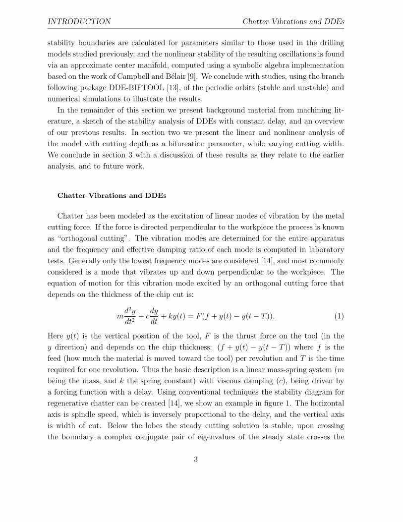
a forcing function with a delay. Using conventional techniques the stability diagram for

regenerative chatter can be created [14], we show an example in figure 1. The horizontal

axis is spindle speed, which is inversely proportional to the delay, and the vertical axis

is width of cut. Below the lobes the steady cutting solution is stable, upon crossing

the boundary a complex conjugate pair of eigenvalues of the steady state crosses the

3

INTRODUCTION Chatter Vibrations and DDEs

0 10 20 30 40 50 60 70 800

5

10

15

spindle speed

wid

th o

f cut

Stability Lobes for Regenerative Chatter

steady cutting solution stable

steady cutting solution unstable

.......

FIG. 1: Stability diagram for regenerative chatter. Steady cutting solution (the trivial solution)

is stable in the region beneath the lobes.

imaginary axis and the stable fixed point becomes an unstable spiral. Similar stability

diagrams can be found in the papers of [15–19], which consider a damped harmonic

oscillator with delayed position and/or velocity dependent feedback.

The Drilling Model

In [1] we report a model for the excitation of two vibration modes seen in twist drills,

the lowest frequency bending mode, which we called the “traditional mode”, and a higher

frequency axial-torsional mode thought to be the cause of striations formed on the bottom

of the hole during high-speed drilling operations. The vibrations are assumed to be linear,

with large inertia and stiffness, and small damping. The equation of motion in η, the

modal amplitude, is hence:

mη + cη + kη = Fη (2)

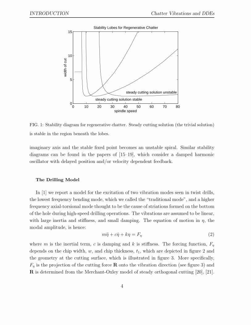
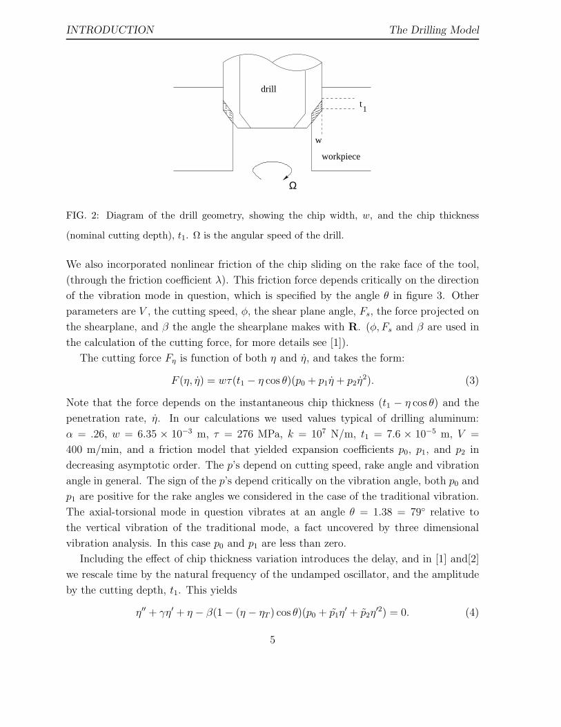
where m is the inertial term, c is damping and k is stiffness. The forcing function, Fη

depends on the chip width, w, and chip thickness, t1, which are depicted in figure 2 and

the geometry at the cutting surface, which is illustrated in figure 3. More specifically,

Fη is the projection of the cutting force R onto the vibration direction (see figure 3) and

R is determined from the Merchant-Oxley model of steady orthogonal cutting [20], [21].

4

INTRODUCTION The Drilling Model

Ω

w

drill

t1

workpiece

FIG. 2: Diagram of the drill geometry, showing the chip width, w, and the chip thickness

(nominal cutting depth), t1. Ω is the angular speed of the drill.

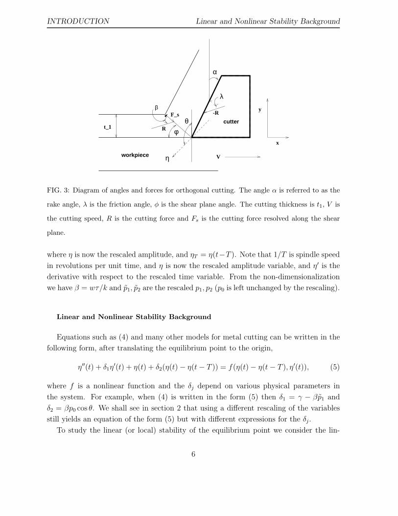
We also incorporated nonlinear friction of the chip sliding on the rake face of the tool,

(through the friction coefficient λ). This friction force depends critically on the direction

of the vibration mode in question, which is specified by the angle θ in figure 3. Other

parameters are V , the cutting speed, φ, the shear plane angle, Fs, the force projected on

the shearplane, and β the angle the shearplane makes with R. (φ, Fs and β are used in

the calculation of the cutting force, for more details see [1]).

The cutting force Fη is function of both η and η, and takes the form:

F (η, η) = wτ(t1 − η cos θ)(p0 + p1η + p2η2). (3)

Note that the force depends on the instantaneous chip thickness (t1 − η cos θ) and the

penetration rate, η. In our calculations we used values typical of drilling aluminum:

α = .26, w = 6.35 × 10−3 m, τ = 276 MPa, k = 107 N/m, t1 = 7.6 × 10−5 m, V =

400 m/min, and a friction model that yielded expansion coefficients p0, p1, and p2 in

decreasing asymptotic order. The p’s depend on cutting speed, rake angle and vibration

angle in general. The sign of the p’s depend critically on the vibration angle, both p0 and

p1 are positive for the rake angles we considered in the case of the traditional vibration.

The axial-torsional mode in question vibrates at an angle θ = 1.38 = 79 relative to

the vertical vibration of the traditional mode, a fact uncovered by three dimensional

vibration analysis. In this case p0 and p1 are less than zero.

Including the effect of chip thickness variation introduces the delay, and in [1] and[2]

we rescale time by the natural frequency of the undamped oscillator, and the amplitude

by the cutting depth, t1. This yields

η′′ + γη′ + η − β(1 − (η − ηT ) cos θ)(p0 + p1η′ + p2η

′2) = 0. (4)

5

INTRODUCTION Linear and Nonlinear Stability Background

y

x

θ

workpiece

cutter

-R

R

F_s

λ

t_1φ

Vη

α

β

FIG. 3: Diagram of angles and forces for orthogonal cutting. The angle α is referred to as the

rake angle, λ is the friction angle, φ is the shear plane angle. The cutting thickness is t1, V is

the cutting speed, R is the cutting force and Fs is the cutting force resolved along the shear

plane.

where η is now the rescaled amplitude, and ηT = η(t−T ). Note that 1/T is spindle speed

in revolutions per unit time, and η is now the rescaled amplitude variable, and η′ is the

derivative with respect to the rescaled time variable. From the non-dimensionalization

we have β = wτ/k and p1, p2 are the rescaled p1, p2 (p0 is left unchanged by the rescaling).

Linear and Nonlinear Stability Background

Equations such as (4) and many other models for metal cutting can be written in the

following form, after translating the equilibrium point to the origin,

η′′(t) + δ1η′(t) + η(t) + δ2(η(t) − η(t − T )) = f(η(t) − η(t − T ), η′(t)), (5)

where f is a nonlinear function and the δj depend on various physical parameters in

the system. For example, when (4) is written in the form (5) then δ1 = γ − βp1 and

δ2 = βp0 cos θ. We shall see in section 2 that using a different rescaling of the variables

still yields an equation of the form (5) but with different expressions for the δj .

To study the linear (or local) stability of the equilibrium point we consider the lin-

6


earization of the model (5)

η′′(t) + δ1η′(t) + η(t) + δ2(η(t) − η(t − T )) = 0. (6)

As is the case for ordinary differential equations, solutions of this linear delay differential

equation may be expressed in the form η(t) = κeλt, where κ, λ ∈ C. Some simple algebra

shows that such solutions will exists if and only if λ is a root the characteristic equation

λ2 + δ1λ + 1 + δ2(1 − e−λT ) = 0. (7)

Note that due to the delay, this is a transcendental equation in λ, which means it will

have a countable infinity of complex roots. Nevertheless, it can be shown [22, 23] that

the stability results from ordinary differential equations hold here as well. Specifically, if

all the roots of (7) have Re(λ) < 0 then the equilibrium point is locally asymptotically

stable and if at least one root has Re(λ) > 0 the the equilibrium point is unstable.

In a physical problem, one is, of course, interested in the dependence of the stability

on the parameters of the system. Using techniques from complex variable theory and

continuity arguments, one can describe regions of parameter space where all the roots of

the characteristic equation have negative real parts. This is usually called the stability

region of the equilibrium point.

In the study of chatter, we are particularly interested in determining the parameter

values where the equilibrium point loses stability, this corresponds to parameter values

where there is at least one root of (7) that satisfies Re(λ) = 0. Such points are said to

define the boundary of the region of stability of the equilibrium point, or the stability

boundary. These points can be found by putting λ = 0 or λ = iω into the characteristic

equation. For chatter problems, the former does not generally occur for physically mean-

ingful parameter values. The latter, however, gives rise to the following (after separating

into real and imaginary parts)

1 − ω2 + δ2(1 − cos ωT ) = 0 (8)

δ1ω + δ2 sin ωT = 0. (9)

These can be further rearranged to give an equation for T as a function of ω and the

other parameters:

T =2

ω

(

arctan

(

1 − ω2

δ1ω

)

+ Nπ

)

, (10)

where N = 0, 1, 2, . . . determines the branch of the arctangent function, and another

equation which is independent of T

(1 − ω2 + δ2)2 + δ2

1ω2 − δ2

2 = 0. (11)

7


From this last equation, we can solve for one of the physical parameters as a function of

ω and the other parameters. For example, if (11) is derived from the model (4), one can

solve for β in terms of the other parameters, since δ1 = γ − βp1 δ2 = βp0 cos θ.

For our general set up, let µ be the physical parameter we solve for. Thus, for fixed

values of the other parameters, (10)–(11) yield parametric equations, T = T (ω), µ =

µ(ω), describing curves in the T, µ parameter space. Along these curves, the characteristic

equation has a pair of pure imaginary roots, thus one may expect that a Hopf bifurcation

occurs. To show that this is indeed the case, one needs to check the transversality and

nonresonance conditions of the Hopf bifurcation Theorem for DDEs [22, pp.331-333].

These conditions may be checked via manipulation of the characteristic equation, (7).

For an example, see the appendix of [2].

Assuming that a Hopf bifurcation does take place as either T or µ is varied through

the curves described by (10)–(11), we now discuss how to determine whether this is a

supercritical or subcritical bifurcation.

To study the criticality of the Hopf bifurcation, it is useful to rewrite the model (5)

as a first order system, viz.,

x′(t) = A0x(t) + A1x(t − T ) + f(x(t),x(t − T )) (12)

where

x(t) =

η(t)

η′(t)

, A0 =

0 1

−(1 + δ2) −δ1

, A1 =

0 0

δ2 0

, (13)

and

f =

0

f(x1(t) − x1(t − T ), x2(t))

. (14)

The linearization of this equation about the trivial solution is

x′(t) = A0x(t) + A1x(t − T ). (15)

It can be shown [22] that the solution space of equations such as (12) and (15) is

infinite dimensional and thus the appropriate phase space for (12) is C def= C([−T, 0], R2),

the space of continuous functions mapping the interval [−T, 0] into R2. The equation

may be recast in terms of this phase space by defining the function

xt(σ)def= x(t + σ), −T ≤ σ ≤ 0,

8


to be the “phase point” at time t. Note that this represents the value of the state x at

time t together with its past history to t − T .

Despite the infinite dimensionality of this phase space, many of the properties of

solutions of delay differential equations such as (12) are similar to those for ordinary

differential equations [22]. In particular, at a Hopf bifurcation point, there exists a two

dimensional centre manifold in the solution space. Further, if all the other roots of the

characteristic equation of the linearization about the equilibrium have negative real parts,

then the centre manifold is attracting and the long term behaviour of solutions to the

nonlinear delay differential equation is well approximated by the flow on this manifold. As

discussed in [9–12] the criticality of the Hopf bifurcation can be determined by studying

the evolution of solutions on the centre manifold. We note that since the manifold is

finite dimensional, this evolution will be described by a system of ordinary differential

equations. In the following we will outline the steps needed to find this system of ordinary

differential equations. Details of the computations for (4) and the theory behind them

can be found in the appendix of [2].

A standard result from the theory of DDEs [22] indicates that the characteristic equa-

tion (7) has at most a finite number of roots with positive real parts. Thus at points

along the curves described by (10)–(11), the trivial solution of (12) has a two dimensional

“centre eigenspace”, N , with basis

Φ(σ) = [φ1(σ), φ2(σ)] =

cos(ωσ) sin(ωσ)

−ω sin(ωσ) ω cos(ωσ)

, (16)

an infinite dimensional “stable eigenspace”, S, and a finite dimensional “unstable

eigenspace”, U .

The corresponding centre manifold is given by

Mf = φ ∈ C | φ = Φu + h(u),

where u = [u1, u2]T are coordinates on N and h(u) ∈ S ⊕ U . Solutions to the DDE (12)

on Mf are given by xt(σ) = Φ(σ)u(t) + h(σ,u(t)), which can be expressed as

xt(σ) =

cos(ωσ)u1(t) + sin(ωσ)u2(t)

−ω sin(ωσ)u1(t) + ω cos(ωσ)u2(t)

+

h111(σ)u1(t)

2 + h112(σ)u1(t)u2(t) + h1

22(σ)u2(t)2

h211(σ)u1(t)

2 + h212(σ)u1(t)u2(t) + h2

22(σ)u2(t)2

+ O(‖u‖3),

9

INTRODUCTION Overview of previous results

where the hijk(σ) are found by solving an ODE boundary value problem as described in

the appendix of [2].

The dynamics on the centre manifold are given by the evolution in time of the coor-

dinates u1(t), u2(t). This is governed by the system of ODEs

u1 = ωu2 + Ψ12(0)(f11u21 + f12u1u2 + f22u

22 + f111u

31 + f112u

21u2 + f122u1u

22 + f222u

32)

u2 = −ωu1 + Ψ22(0)(f11u21 + f12u1u2 + f22u

22 + f111u

31 + f112u

21u2 + f122u1u

22 + f222u

32)

+O(‖u‖4).

The Ψij(0) are functions of the physical parameters of the system, and of the Hopf

frequency, ω. The fij, fijk are functions of these and the centre manifold coefficients

hijk(0) and hi

jk(−T ).

Using the result given in [24, p. 152], it is easily shown that the criticality of the Hopf

bifurcation is determined by the sign of the following quantity

a =1

8[Ψ12(0)(3f111 + f122) + Ψ22(0)(f112 + 3f222)]

− 1

8ω

[

(Ψ12(0)2 −Ψ22(0)2)f12(f11 + f22) + 2Ψ12(0)Ψ22(0)(f 222 − f 2

11)]

.(17)

If a < 0 then the Hopf bifurcation is supercritical and if a > 0 it is subcritical. If a = 0

the criticality is not determined by the third order terms of the equation.

Although these computations are long, they can be automated in a symbolic algebra

package such as Maple [9]. From this one obtains an expression for a as a function of the

physical parameters and the Hopf frequency, ω. This expression can then be evaluated

at points along the curves described by (10)–(11), and in particular along the stability

boundary, to determine if the Hopf bifurcation is super- or subcritical.

Overview of previous results

In [1] we determined linear stability boundaries for the drilling model for both the

axial-torsional and traditional vibration mode. There we solved (4) for T and β as

functions of ω, and in terms of these variables equations (11) and (10) are written

p21ω

2β2 − ((ω2 − 1)(2p0 cos θ) + 2γp1ω2)β + (γ2ω2 + (ω2 − 1)2) = 0. (18)

and

T (ω) =2

ω(arctan(

1 − ω2

(γ − βp1)ω) + Nπ). (19)

For the axial-torsional case positive solutions for β occur for values of ω between zero

and 1, and for the traditional case, for values of ω greater than 1, indicating that the

10


0 0.1 0.2 0.3 0.4 0.5 0.60

5

10

β

Stability boundaries, p0=0.8, p

1=0.2, γ=0.5, traditional case

0 2 4 6 8 100

10

20

30

β

1/T

0 0.2 0.4 0.6 0.8 10

10

20

30

β

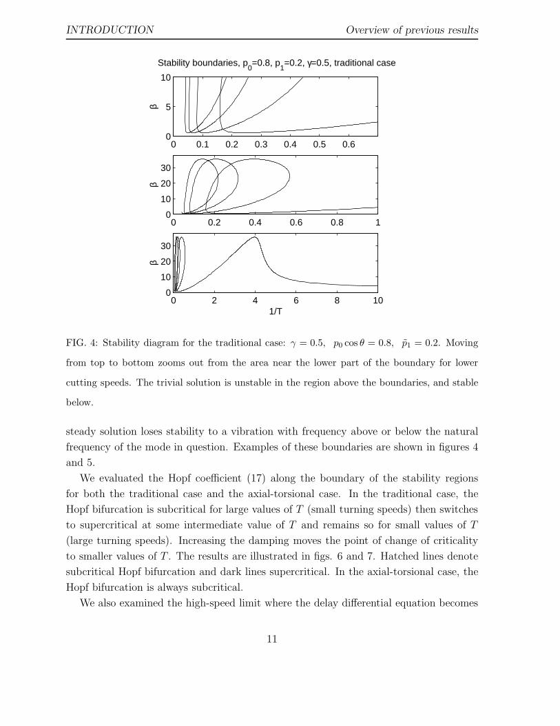
FIG. 4: Stability diagram for the traditional case: γ = 0.5, p0 cos θ = 0.8, p1 = 0.2. Moving

from top to bottom zooms out from the area near the lower part of the boundary for lower

cutting speeds. The trivial solution is unstable in the region above the boundaries, and stable

below.

steady solution loses stability to a vibration with frequency above or below the natural

frequency of the mode in question. Examples of these boundaries are shown in figures 4

and 5.

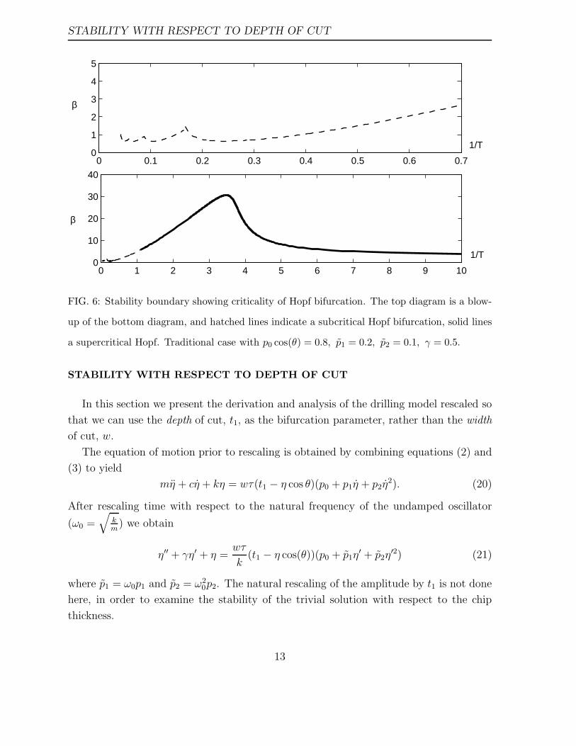
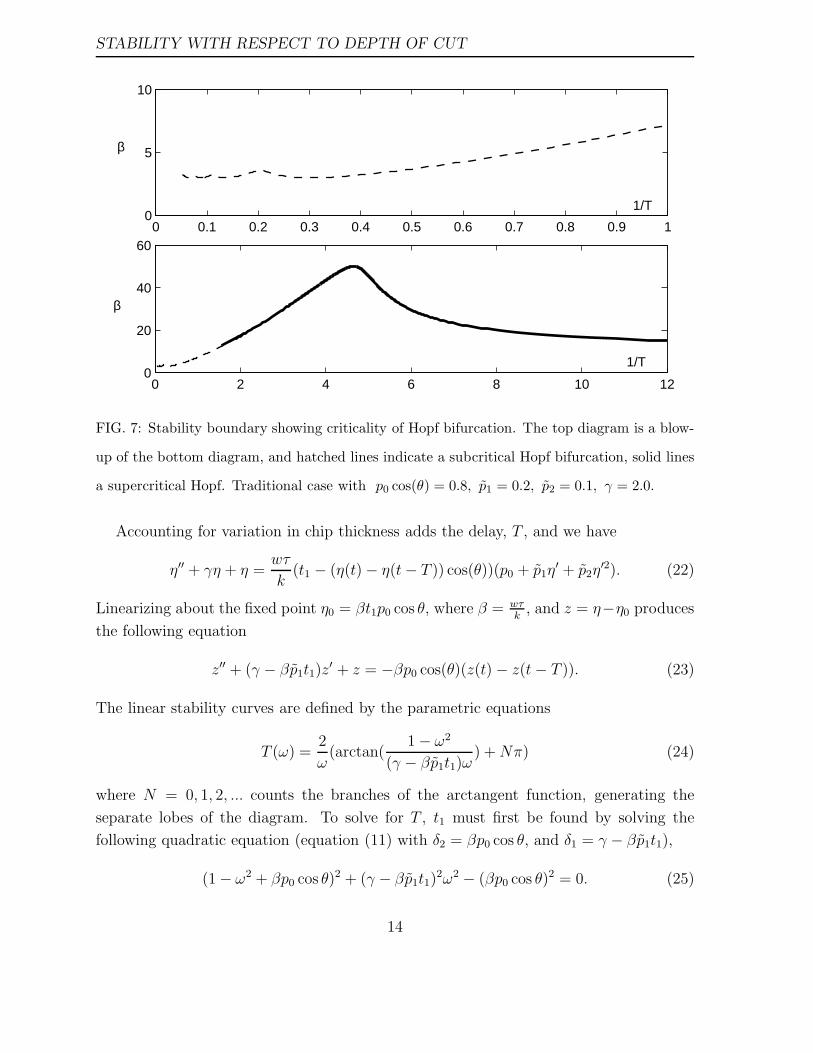
We evaluated the Hopf coefficient (17) along the boundary of the stability regions

for both the traditional case and the axial-torsional case. In the traditional case, the

Hopf bifurcation is subcritical for large values of T (small turning speeds) then switches

to supercritical at some intermediate value of T and remains so for small values of T

(large turning speeds). Increasing the damping moves the point of change of criticality

to smaller values of T . The results are illustrated in figs. 6 and 7. Hatched lines denote

subcritical Hopf bifurcation and dark lines supercritical. In the axial-torsional case, the

Hopf bifurcation is always subcritical.

We also examined the high-speed limit where the delay differential equation becomes

11


0 0.2 0.4 0.6 0.8 10

0.5

1

1.5

2

2.5

Stability boundaries, p0=−0.8, p

1=−0.4, γ=0.5, axial−torsional case

β

0 0.05 0.1 0.150.5

0.55

0.6

0.65

0.7

0.75

β

1/T

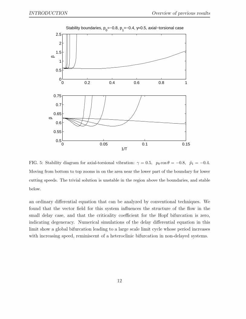
FIG. 5: Stability diagram for axial-torsional vibration: γ = 0.5, p0 cos θ = −0.8, p1 = −0.4.

Moving from bottom to top zooms in on the area near the lower part of the boundary for lower

cutting speeds. The trivial solution is unstable in the region above the boundaries, and stable

below.

an ordinary differential equation that can be analyzed by conventional techniques. We

found that the vector field for this system influences the structure of the flow in the

small delay case, and that the criticality coefficient for the Hopf bifurcation is zero,

indicating degeneracy. Numerical simulations of the delay differential equation in this

limit show a global bifurcation leading to a large scale limit cycle whose period increases

with increasing speed, reminiscent of a heteroclinic bifurcation in non-delayed systems.

12

STABILITY WITH RESPECT TO DEPTH OF CUT

0 0.1 0.2 0.3 0.4 0.5 0.6 0.70

1

2

3

4

5

1/T

β

0 1 2 3 4 5 6 7 8 9 100

10

20

30

40

1/T

β

FIG. 6: Stability boundary showing criticality of Hopf bifurcation. The top diagram is a blow-

up of the bottom diagram, and hatched lines indicate a subcritical Hopf bifurcation, solid lines

a supercritical Hopf. Traditional case with p0 cos(θ) = 0.8, p1 = 0.2, p2 = 0.1, γ = 0.5.


In this section we present the derivation and analysis of the drilling model rescaled so

that we can use the depth of cut, t1, as the bifurcation parameter, rather than the width

of cut, w.

The equation of motion prior to rescaling is obtained by combining equations (2) and

(3) to yield

mη + cη + kη = wτ(t1 − η cos θ)(p0 + p1η + p2η2). (20)

After rescaling time with respect to the natural frequency of the undamped oscillator

(ω0 =√

km

) we obtain

η′′ + γη′ + η =wτ

k(t1 − η cos(θ))(p0 + p1η

′ + p2η′2) (21)

where p1 = ω0p1 and p2 = ω20p2. The natural rescaling of the amplitude by t1 is not done

here, in order to examine the stability of the trivial solution with respect to the chip

thickness.

13


0 0.1 0.2 0.3 0.4 0.5 0.6 0.7 0.8 0.9 10

5

10

1/T

β

0 2 4 6 8 10 120

20

40

60

1/T

β

FIG. 7: Stability boundary showing criticality of Hopf bifurcation. The top diagram is a blow-

up of the bottom diagram, and hatched lines indicate a subcritical Hopf bifurcation, solid lines

a supercritical Hopf. Traditional case with p0 cos(θ) = 0.8, p1 = 0.2, p2 = 0.1, γ = 2.0.

Accounting for variation in chip thickness adds the delay, T , and we have

η′′ + γη + η =wτ

k(t1 − (η(t) − η(t − T )) cos(θ))(p0 + p1η

′ + p2η′2). (22)

Linearizing about the fixed point η0 = βt1p0 cos θ, where β = wτk

, and z = η−η0 produces

the following equation

z′′ + (γ − βp1t1)z′ + z = −βp0 cos(θ)(z(t) − z(t − T )). (23)

The linear stability curves are defined by the parametric equations

T (ω) =2

ω(arctan(

1 − ω2

(γ − βp1t1)ω) + Nπ) (24)

where N = 0, 1, 2, ... counts the branches of the arctangent function, generating the

separate lobes of the diagram. To solve for T , t1 must first be found by solving the

following quadratic equation (equation (11) with δ2 = βp0 cos θ, and δ1 = γ − βp1t1),

(1 − ω2 + βp0 cos θ)2 + (γ − βp1t1)2ω2 − (βp0 cos θ)2 = 0. (25)

14


Conditions for a real solution to this quadratic in t1 determine allowable ranges of the

parameter ω, and depend on the values of β, p0 and γ. Specifically,

t±1 =γ

p1β±

√

(ω2 − 1)(1 + 2βp0 cos(θ) − ω2)

p1βω, (26)

so that t1 will be a real valued-function of ω when either ω2−1 > 0 and 1+2βp0 cos(θ)−ω2 > 0, or both when both expressions are < 0. The former implies the range 1 < ω2 <

1 + 2βp0 cos(θ), hence also requires that p0 cos(θ) > 0, which occurs in the traditional

vibration case. The latter set of inequalities combines to give 1 + 2βp0 cos(θ) < ω2 < 1,

which can be satisfied if p0 cos(θ) < 0, which occurs in the axial-torsional vibration case.

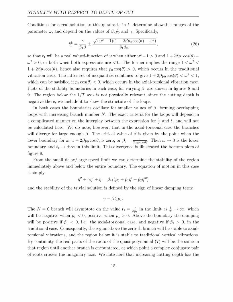
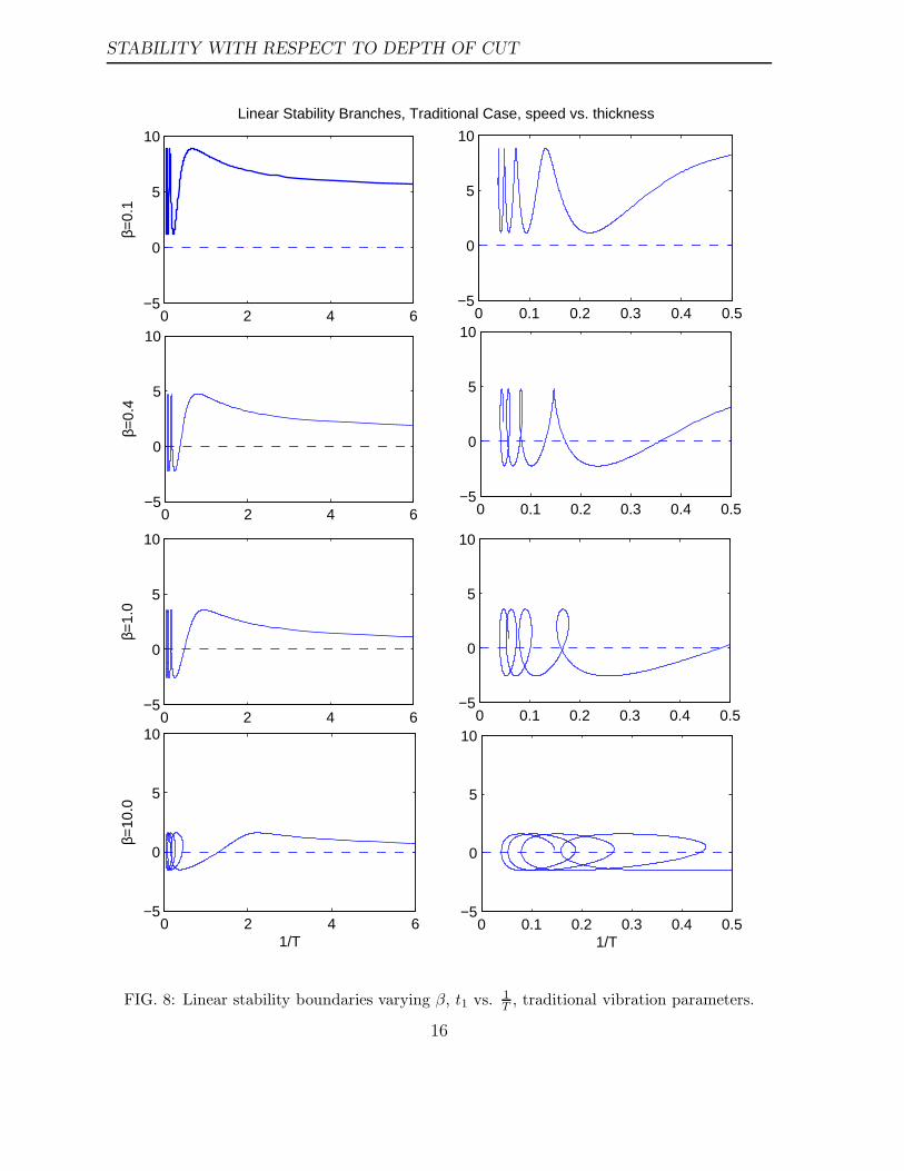
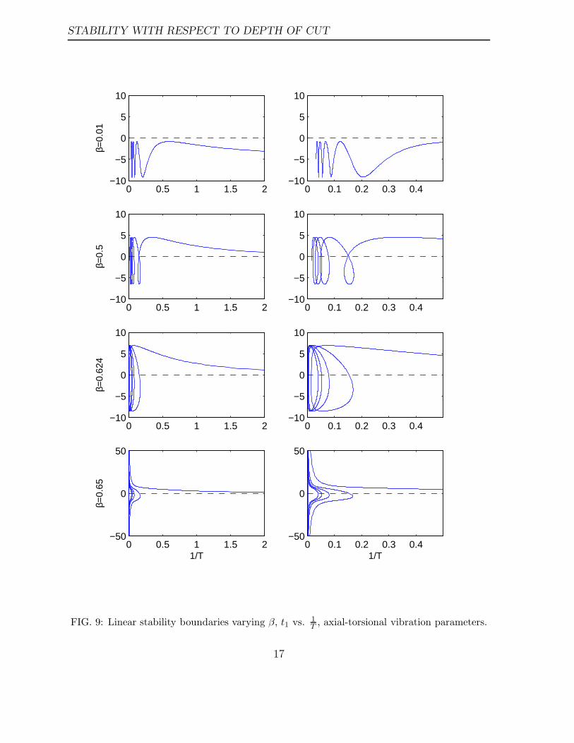
Plots of the stability boundaries in each case, for varying β, are shown in figures 8 and

9. The region below the 1/T axis is not physically relevant, since the cutting depth is

negative there, we include it to show the structure of the loops.

In both cases the boundaries oscillate for smaller values of β, forming overlapping

loops with increasing branch number N . The exact criteria for the loops will depend in

a complicated manner on the interplay between the expression for 1T

and t1 and will not

be calculated here. We do note, however, that in the axial-torsional case the branches

will diverge for large enough β. The critical value of β is given by the point when the

lower boundary for ω, 1 + 2βp0 cos θ, is zero, or βc = 12|p0 cos θ|

. Then ω → 0 is the lower

boundary and t1 → ±∞ in this limit. This divergence is illustrated the bottom plots of

figure 9.

From the small delay/large speed limit we can determine the stability of the region

immediately above and below the entire boundary. The equation of motion in this case

is simply

η′′ + γη′ + η = βt1(p0 + p1η′ + p2η

′2)

and the stability of the trivial solution is defined by the sign of linear damping term:

γ − βt1p1.

The N = 0 branch will asymptote on the value t1 = γβp1

in the limit as 1T→ ∞. which

will be negative when p1 < 0, positive when p1 > 0. Above the boundary the damping

will be positive if p1 < 0, i.e. the axial-torsional case, and negative if p1 > 0, in the

traditional case. Consequently, the region above the zero-th branch will be stable to axial-

torsional vibrations, and the region below it is stable to traditional vertical vibrations.

By continuity the real parts of the roots of the quasi-polynomial (7) will be the same in

that region until another branch is encountered, at which point a complex conjugate pair

of roots crosses the imaginary axis. We note here that increasing cutting depth has the

15


0 2 4 6−5

0

5

10β=

0.1

Linear Stability Branches, Traditional Case, speed vs. thickness

0 0.1 0.2 0.3 0.4 0.5−5

0

5

10

0 2 4 6−5

0

5

10

β=0.

4

0 0.1 0.2 0.3 0.4 0.5−5

0

5

10

0 2 4 6−5

0

5

10

β=1.

0

0 0.1 0.2 0.3 0.4 0.5−5

0

5

10

0 2 4 6−5

0

5

10

1/T

β=10

.0

0 0.1 0.2 0.3 0.4 0.5−5

0

5

10

1/T

FIG. 8: Linear stability boundaries varying β, t1 vs. 1T , traditional vibration parameters.

16


0 0.5 1 1.5 2−10

−5

0

5

10β=

0.01

0 0.1 0.2 0.3 0.4−10

−5

0

5

10

0 0.5 1 1.5 2−10

−5

0

5

10

β=0.

5

0 0.1 0.2 0.3 0.4−10

−5

0

5

10

0 0.5 1 1.5 2−10

−5

0

5

10

β=0.

624

0 0.1 0.2 0.3 0.4−10

−5

0

5

10

0 0.5 1 1.5 2−50

0

50

1/T

β=0.

65

0 0.1 0.2 0.3 0.4−50

0

50

1/T

FIG. 9: Linear stability boundaries varying β, t1 vs. 1T , axial-torsional vibration parameters.

17


0 0.2 0.4 0.6 0.8 1 1.2 1.4 1.6−6

−4

−2

0

2

4

6

8

β

t 1

Extrema for stability boundary, Traditional case

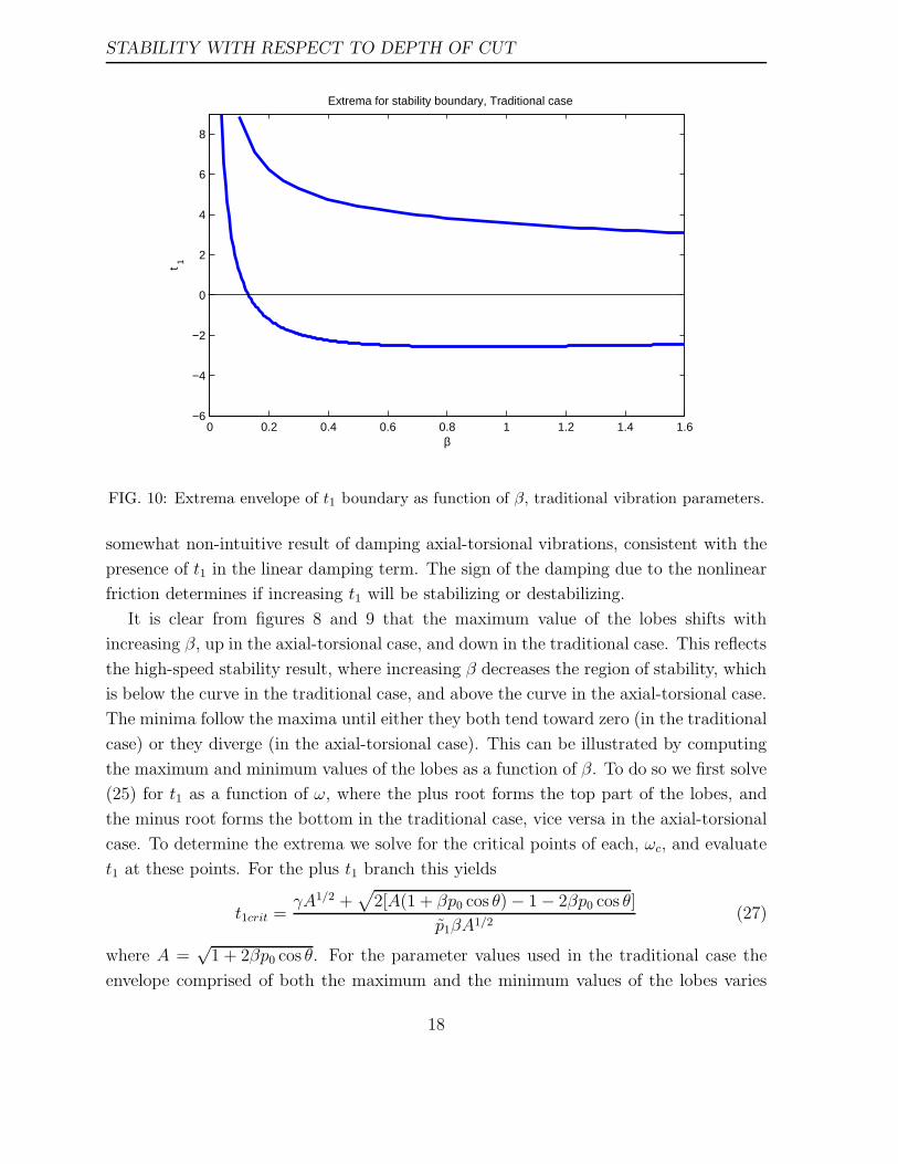
FIG. 10: Extrema envelope of t1 boundary as function of β, traditional vibration parameters.

somewhat non-intuitive result of damping axial-torsional vibrations, consistent with the

presence of t1 in the linear damping term. The sign of the damping due to the nonlinear

friction determines if increasing t1 will be stabilizing or destabilizing.

It is clear from figures 8 and 9 that the maximum value of the lobes shifts with

increasing β, up in the axial-torsional case, and down in the traditional case. This reflects

the high-speed stability result, where increasing β decreases the region of stability, which

is below the curve in the traditional case, and above the curve in the axial-torsional case.

The minima follow the maxima until either they both tend toward zero (in the traditional

case) or they diverge (in the axial-torsional case). This can be illustrated by computing

the maximum and minimum values of the lobes as a function of β. To do so we first solve

(25) for t1 as a function of ω, where the plus root forms the top part of the lobes, and

the minus root forms the bottom in the traditional case, vice versa in the axial-torsional

case. To determine the extrema we solve for the critical points of each, ωc, and evaluate

t1 at these points. For the plus t1 branch this yields

t1crit =γA1/2 +

√

2[A(1 + βp0 cos θ) − 1 − 2βp0 cos θ]

p1βA1/2(27)

where A =√

1 + 2βp0 cos θ. For the parameter values used in the traditional case the

envelope comprised of both the maximum and the minimum values of the lobes varies

18

STABILITY WITH RESPECT TO DEPTH OF CUT Nonlinear Stability

0 0.1 0.2 0.3 0.4 0.5 0.6−20

−15

−10

−5

0

5

10

β

Max

t1

Extrema of Stability Boundary, Axial−Torsional case

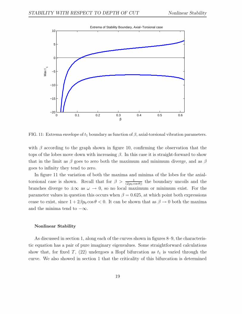
FIG. 11: Extrema envelope of t1 boundary as function of β, axial-torsional vibration parameters.

with β according to the graph shown in figure 10, confirming the observation that the

tops of the lobes move down with increasing β. In this case it is straight-forward to show

that in the limit as β goes to zero both the maximum and minimum diverge, and as β

goes to infinity they tend to zero.

In figure 11 the variation of both the maxima and minima of the lobes for the axial-

torsional case is shown. Recall that for β > 1(2|p0 cos θ|)

the boundary uncoils and the

branches diverge to ±∞ as ω → 0, so no local maximum or minimum exist. For the

parameter values in question this occurs when β = 0.625, at which point both expressions

cease to exist, since 1 + 2βp0 cos θ < 0. It can be shown that as β → 0 both the maxima

and the minima tend to −∞.

Nonlinear Stability

As discussed in section 1, along each of the curves shown in figures 8–9, the characteris-

tic equation has a pair of pure imaginary eigenvalues. Some straightforward calculations

show that, for fixed T , (22) undergoes a Hopf bifurcation as t1 is varied through the

curve. We also showed in section 1 that the criticality of this bifurcation is determined

19


–4

–2

0

2

4

6

8

10

t1

0.1 0.2 0.3 0.4 0.5

1/T

(a)

–4

–2

0

2

4

6

8

10

t1

0.1 0.2 0.3 0.4 0.5

1/T

(b)

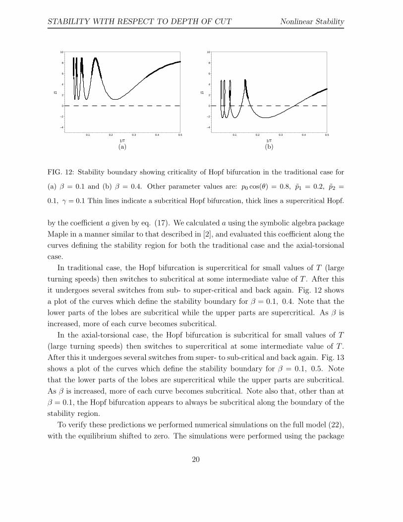
FIG. 12: Stability boundary showing criticality of Hopf bifurcation in the traditional case for

(a) β = 0.1 and (b) β = 0.4. Other parameter values are: p0 cos(θ) = 0.8, p1 = 0.2, p2 =

0.1, γ = 0.1 Thin lines indicate a subcritical Hopf bifurcation, thick lines a supercritical Hopf.

by the coefficient a given by eq. (17). We calculated a using the symbolic algebra package

Maple in a manner similar to that described in [2], and evaluated this coefficient along the

curves defining the stability region for both the traditional case and the axial-torsional

case.

In traditional case, the Hopf bifurcation is supercritical for small values of T (large

turning speeds) then switches to subcritical at some intermediate value of T . After this

it undergoes several switches from sub- to super-critical and back again. Fig. 12 shows

a plot of the curves which define the stability boundary for β = 0.1, 0.4. Note that the

lower parts of the lobes are subcritical while the upper parts are supercritical. As β is

increased, more of each curve becomes subcritical.

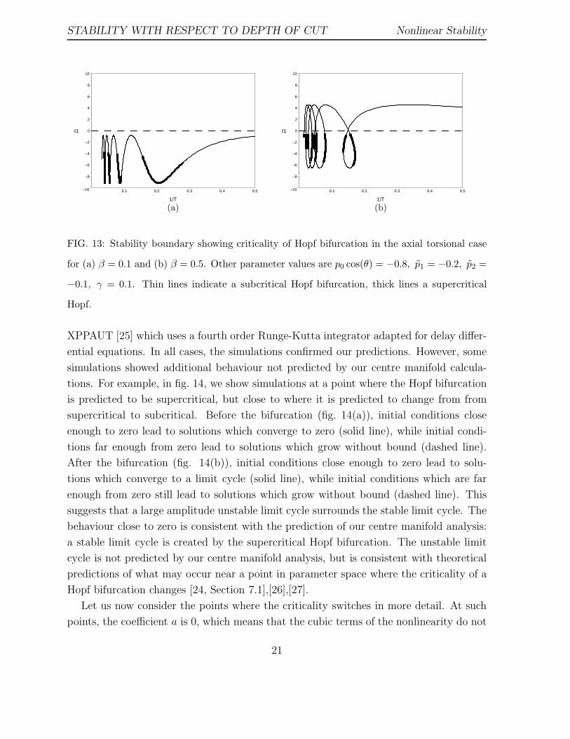
In the axial-torsional case, the Hopf bifurcation is subcritical for small values of T

(large turning speeds) then switches to supercritical at some intermediate value of T .

After this it undergoes several switches from super- to sub-critical and back again. Fig. 13

shows a plot of the curves which define the stability boundary for β = 0.1, 0.5. Note

that the lower parts of the lobes are supercritical while the upper parts are subcritical.

As β is increased, more of each curve becomes subcritical. Note also that, other than at

β = 0.1, the Hopf bifurcation appears to always be subcritical along the boundary of the

stability region.

To verify these predictions we performed numerical simulations on the full model (22),

with the equilibrium shifted to zero. The simulations were performed using the package

20


–10

–8

–6

–4

–2

0

2

4

6

8

10

t1

0.1 0.2 0.3 0.4 0.5

1/T

(a)

–10

–8

–6

–4

–2

0

2

4

6

8

10

t1

0.1 0.2 0.3 0.4 0.5

1/T

(b)

FIG. 13: Stability boundary showing criticality of Hopf bifurcation in the axial torsional case

for (a) β = 0.1 and (b) β = 0.5. Other parameter values are p0 cos(θ) = −0.8, p1 = −0.2, p2 =

−0.1, γ = 0.1. Thin lines indicate a subcritical Hopf bifurcation, thick lines a supercritical

Hopf.

XPPAUT [25] which uses a fourth order Runge-Kutta integrator adapted for delay differ-

ential equations. In all cases, the simulations confirmed our predictions. However, some

simulations showed additional behaviour not predicted by our centre manifold calcula-

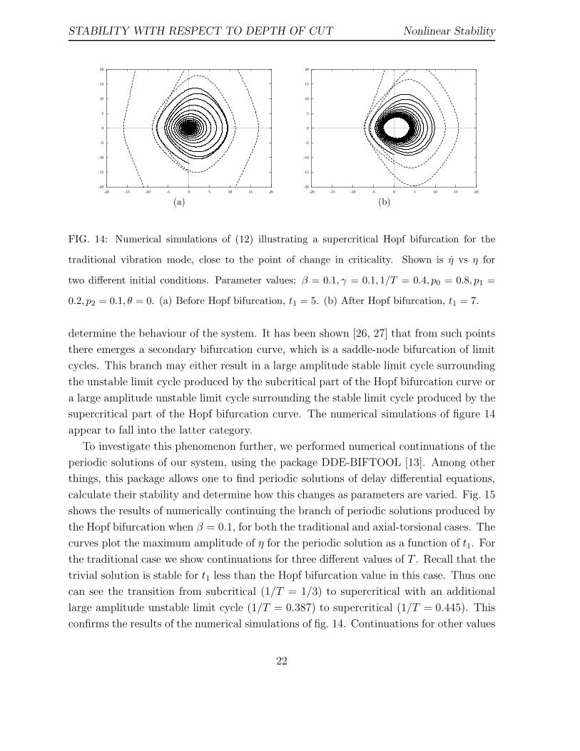
tions. For example, in fig. 14, we show simulations at a point where the Hopf bifurcation

is predicted to be supercritical, but close to where it is predicted to change from from

supercritical to subcritical. Before the bifurcation (fig. 14(a)), initial conditions close

enough to zero lead to solutions which converge to zero (solid line), while initial condi-

tions far enough from zero lead to solutions which grow without bound (dashed line).

After the bifurcation (fig. 14(b)), initial conditions close enough to zero lead to solu-

tions which converge to a limit cycle (solid line), while initial conditions which are far

enough from zero still lead to solutions which grow without bound (dashed line). This

suggests that a large amplitude unstable limit cycle surrounds the stable limit cycle. The

behaviour close to zero is consistent with the prediction of our centre manifold analysis:

a stable limit cycle is created by the supercritical Hopf bifurcation. The unstable limit

cycle is not predicted by our centre manifold analysis, but is consistent with theoretical

predictions of what may occur near a point in parameter space where the criticality of a

Hopf bifurcation changes [24, Section 7.1],[26],[27].

Let us now consider the points where the criticality switches in more detail. At such

points, the coefficient a is 0, which means that the cubic terms of the nonlinearity do not

21


-20

-15

-10

-5

0

5

10

15

20

-20 -15 -10 -5 0 5 10 15 20

(a)

-20

-15

-10

-5

0

5

10

15

20

-20 -15 -10 -5 0 5 10 15 20

(b)

FIG. 14: Numerical simulations of (12) illustrating a supercritical Hopf bifurcation for the

traditional vibration mode, close to the point of change in criticality. Shown is η vs η for

two different initial conditions. Parameter values: β = 0.1, γ = 0.1, 1/T = 0.4, p0 = 0.8, p1 =

0.2, p2 = 0.1, θ = 0. (a) Before Hopf bifurcation, t1 = 5. (b) After Hopf bifurcation, t1 = 7.

determine the behaviour of the system. It has been shown [26, 27] that from such points

there emerges a secondary bifurcation curve, which is a saddle-node bifurcation of limit

cycles. This branch may either result in a large amplitude stable limit cycle surrounding

the unstable limit cycle produced by the subcritical part of the Hopf bifurcation curve or

a large amplitude unstable limit cycle surrounding the stable limit cycle produced by the

supercritical part of the Hopf bifurcation curve. The numerical simulations of figure 14

appear to fall into the latter category.

To investigate this phenomenon further, we performed numerical continuations of the

periodic solutions of our system, using the package DDE-BIFTOOL [13]. Among other

things, this package allows one to find periodic solutions of delay differential equations,

calculate their stability and determine how this changes as parameters are varied. Fig. 15

shows the results of numerically continuing the branch of periodic solutions produced by

the Hopf bifurcation when β = 0.1, for both the traditional and axial-torsional cases. The

curves plot the maximum amplitude of η for the periodic solution as a function of t1. For

the traditional case we show continuations for three different values of T . Recall that the

trivial solution is stable for t1 less than the Hopf bifurcation value in this case. Thus one

can see the transition from subcritical (1/T = 1/3) to supercritical with an additional

large amplitude unstable limit cycle (1/T = 0.387) to supercritical (1/T = 0.445). This

confirms the results of the numerical simulations of fig. 14. Continuations for other values

22


0 1 2 3 4 5 6 7 8 9 100

5

10

max

(x)

1/T=1/3

0 1 2 3 4 5 6 7 8 9 100

5

10

max

(x)

1/T=0.387

0 1 2 3 4 5 6 7 8 9 100

5

10

t1

max

(x)

1/T=0.445

(a)

−8 −7 −6 −5 −4 −3 −2 −1 0 1 20

20

40

max

(η)

1/T=0.15

−8 −7 −6 −5 −4 −3 −2 −1 0 1 20

20

40

max

(η)

1/T=0.16

−8 −7 −6 −5 −4 −3 −2 −1 0 1 20

20

40

max

(η)

1/T=0.25

−8 −7 −6 −5 −4 −3 −2 −1 0 1 20

20

40

t1

max

(η)

1/T=0.3

(b)

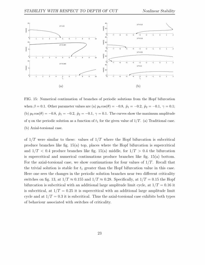
FIG. 15: Numerical continuation of branches of periodic solutions from the Hopf bifurcation

when β = 0.1. Other parameter values are (a) p0 cos(θ) = −0.8, p1 = −0.2, p2 = −0.1, γ = 0.1;

(b) p0 cos(θ) = −0.8, p1 = −0.2, p2 = −0.1, γ = 0.1. The curves show the maximum amplitude

of η on the periodic solution as a function of t1 for the given value of 1/T . (a) Traditional case.

(b) Axial-torsional case.

of 1/T were similar to these: values of 1/T where the Hopf bifurcation is subcritical

produce branches like fig. 15(a) top, places where the Hopf bifurcation is supercritical

and 1/T < 0.4 produce branches like fig. 15(a) middle, for 1/T > 0.4 the bifurcation

is supercritical and numerical continuations produce branches like fig. 15(a) bottom.

For the axial-torsional case, we show continuations for four values of 1/T . Recall that

the trivial solution is stable for t1 greater than the Hopf bifurcation value in this case.

Here one sees the changes in the periodic solution branches near two different criticality

switches on fig. 13, at 1/T ≈ 0.155 and 1/T ≈ 0.28. Specifically, at 1/T = 0.15 the Hopf

bifurcation is subcritical with an additional large amplitude limit cycle, at 1/T = 0.16 it

is subcritical, at 1/T = 0.25 it is supercritical with an additional large amplitude limit

cycle and at 1/T = 0.3 it is subcritical. Thus the axial-torsional case exhibits both types

of behaviour associated with switches of criticality.

23

DISCUSSION AND CONCLUSIONS


For the purposes of machining, system parameters that can be varied easily are cutting

width, thickness and cutting speed. We illustrate the effect of varying thickness and speed

with linear stability boundaries in the (1/T, t1) plane, and consider the way this changes

with varying cutting width. While the standard analysis of the delay differential equation

that describes chatter in metal cutting shows similar stability lobes, they are created by

varying the cutting width.

Adding nonlinear forcing due to nonlinear friction on the rake face of the tool, and

introducing varying angle of vibration generates significantly different stability lobes that

usually studied, most easily seen is the presence of closed loops. This, while interesting

mathematically, is not as pertinent as the effect of varying vibration angle on the whole

picture, which leads to such observations as the frequency of induced vibration must

be less than the natural frequency of the axial-torsional mode, and the reverse for the

traditional vertical vibration mode. Close to the boundaries either a stable or unstable

limit cycle will exist, and the nonlinear stability analysis we perform here uncovers this

distinction. We find that the traditional case is supercritical for large cutting speed,

with several switches between super- and subcritical for smaller cutting speeds. The

axial-torsional case also has switches between super- and subcritical, but these all occur

for negative values of t1, thus the Hopf bifurcation is always subcritical for physically

reasonable values of t1.

The switch from sub- to supercritical bifurcation along a boundary indicates a degen-

eracy in the Hopf coefficient, meaning that higher order terms are needed to determine

the stability at that point. A numerical continuation package can give some indication of

global picture during these transitions, however, and we see a saddle node bifurcation of

the limit cycle occurs at intermediate parameter values. This is validated by numerical

simulations of the DDE which show a stable limit cycle enclosed by an unstable cycle for

appropriate parameter values in the traditional case.

Numerical continuation can also show that phenomena that occur for nonphysical

parameter values influences the behaviour for physically relevant parameter values. The

most striking example we found is a situation where linear stability analysis indicates

the equilibrium solution is stable for t1 > 0, i.e. all physically reasonable values of the

cutting thickness. Since the stability boundary and associated Hopf bifurcation lie in the

region t1 < 0, one might assume that it has no influence on the behaviour of the physical

system. However, numerical continuations show that unstable periodic solutions which

are generated by Hopf bifurcations for t1 < 0 persist when t1 > 0 and thus can affect the

24


behaviour of the physical system.

The implications of switching from a supercritical to subcritical Hopf from a machin-

ing stand-point concern the accuracy of the stability boundaries in the linear stability

diagram. When a supercritical Hopf is encountered the linear stability boundary deter-

mines where the steady cutting solution goes unstable, but if the Hopf is subcritical, the

existence of the small unstable cycle near the steady cutting solution means that small

perturbations could push the trajectory out past the cycle and into a region of instability.

Noise in the system then will blur boundaries, rendering them much less accurate.

This study suggests further mathematical investigation of the global bifurcations of

such DDE systems, which would be needed to fully explain the switching behaviour seen

in fig. 15. The theory of global bifurcation in DDEs with a constant delay term has

not been mapped out, and the development of such a framework would be a significant

advance in the understanding on nonlinear DDEs.

Acknowledgements

This research was supported by the Natural Sciences and Engineering Research Coun-

cil of Canada (grant no. 171089) and by the NSF-EPSCoR program at the University of

Montana.

[1] Stone, E., and Askari, A., 2002. “Nonlinear Models of Chatter in Drilling Processes”.

Dynamical Systems, 17(1), pp. 65–85.

[2] Stone, E., and Campbell, S. A., 2004. “Stability and Bifurcation Analysis of a Nonlinear

DDE Model for Drilling”. J. Nonlinear Science, 14(1), pp. 27–57.

[3] Tlusty, J., 1986. “The Dynamics of High-Speed Milling”. J. Eng. Ind., 108, pp. 59–67.

[4] Altintas, Y., and Budak, E., 1995. “Analytical Prediction of Stability Lobes in Milling”.

Annals of the CIRP, 44(1), pp. 357–362.

[5] Bayly, P. V., Metzler, S. A., Schaut, A. J., and Young, K. A., 2001. “Theory of Torsional

Chatter in Twist Drills: Model, Stability Analysis and Comparison to Test”. ASME J.

Man. Sci. & Eng., 123, pp. 552–561.

25


[6] Bayly, P. V., Young, K. A., and Halley, J. E., 2001. “Analysis of Tool Oscillation and Hole

Roundness Error in a Quasi-Static Model of Reaming”. ASME J. Man. Sci. & Eng., 123,

pp. 387–396.

[7] Stepan, G., 1989. Retarded Dynamical Systems: Stability and Characteristic Functions.

Longman Group, Essex.

[8] Stepan, G., 1998. “Delay-Differential Equation Models for Machine Tool Chatter”. In

Dynamics and Chaos in Manufacturing Processes, F. Moon, ed. J. Wiley, New York,

pp. 165–191.

[9] Campbell, S. A., and Belair, J., 1995. “Analytical and Symbolically-Assisted Investigation

of Hopf Bifurcations in Delay-Differential Equations”. Can. Appl. Math. Quart., 3(2),

pp. 137–154.

[10] Faria, T., and Magalhaes, L., 1995. “Normal Forms for Retarded Functional Differential

Equations with Parameters and Applications to Hopf Bifurcation”. JDE, 122, pp. 181–200.

[11] Hale, J. K., 1985. “Flows on Center Manifolds for Scalar Functional Differential Equa-

tions”. Proc. Roy. Soc. Edinburgh, 101A, pp. 193–201.

[12] Wischert, W., Wunderlin, A., Pelster, A., Olivier, M., and Groslambert, J., 1994. “Delay-

Induced Instabilities in Nonlinear Feedback Systems”. Phys. Rev. E, 49(1), pp. 203–219.

[13] Engelborghs, K., Luzyanina, T., and Samaey, G., 2001. “DDE-BIFTOOL v. 2.00: a Matlab

Package for Bifurcation Analysis of Delay Differential Equations.”. Tech. Rep. TW-330,

Department of Computer Science, K.U. Leuven, Leuven, Belgium.

[14] Tobias, S. A., 1965. Machine Tool Vibration. J. Wiley, New York.

[15] Bhatt, S. J., and Hsu, C. S., 1966. “Stability Criteria for Second Order Dynamical Systems

with Time Lag.”. J. App. Mech., 33, pp. 113–118.

[16] Campbell, S. A., 1999. “Stability and Bifurcation in the Harmonic Oscillator with Multiple

Delayed Feedback Loops.”. Dyn. Cont. Disc. Impul. Sys., 5, pp. 225–235.

[17] Campbell, S. A., Belair, J., Ohira, T., and Milton, J., 1995. “Limit Cycles, Tori, and Com-

plex Dynamics in a Second-Order Differential Equations with Delayed Negative Feedback”.

J. Dyn. Diff. Eqs., 7(1), pp. 213–236.

26


[18] Cooke, K. L., and Grossman, Z., 1982. “Discrete Delay, Distributed Delay and Stability

Switches”. J. Math. Anal. Appl., 86, pp. 592–627.

[19] Hsu, C. S., and Bhatt, S. J., 1966. “Stability Charts for Second-Order Dynamical Systems

with Time Lag.”. J. Appl. Mech., 33, pp. 119–124.

[20] Merchant, M. E., 1945. “Mechanics of the Cutting Process. I. Orthogonal Cutting and a

Type 2 Chip”. J. Appl. Phys., 16, pp. 267–275.

[21] Oxley, P. L. B., 1989. The Mechanics of Machining: an Analytical Approach to Assessing

Machinability. Ellis Horwood, Chichester, England.

[22] Hale, J. K., and Verduyn Lunel, S. M., 1993. Introduction to Functional Differential

Equations. Springer Verlag, New York.

[23] Kolmanovskii, V. B., and Nosov, V. R., 1986. Stability of Functional Differential Equations.

Academic Press, London, England.

[24] Guckenheimer, J., and Holmes, P. J., 1993. Nonlinear Oscillations, Dynamical Systems

and Bifurcations of Vector Fields. Springer-Verlag, New York.

[25] Ermentrout, G. B., 2002. Simulating, Analyzing and Animating Dynamical Systems: A

Guide to XPPAUT for Researcher and Students. SIAM, Philadelphia, PA.

[26] Golubitsky, M., and Langford, W. F., 1981. “Classification and Unfoldings of Degenerate

Hopf Bifurcation”. JDE, 41, pp. 525–546.

[27] Takens, F., 1973. “Unfoldings of Certain Singularities of Vector Fields: Generalized Hopf

Bifurcations”. JDE, 14, pp. 476–493.

27

analysis of the chatter instability in a nonlinear model

Documents