analysis of the behaviour of geogrid-anchored sheet pile walls
TRANSCRIPT

Analysis of the behaviour of geogrid-anchored sheet pile walls
Small-scale experiments and 2D PLAXIS analysis.
Delft University of Technology
Department of Geosciences and Engineering
MSc Thesis Report
Date colloquium: Thursday September 3, 2020
Author:
Britt Wittekoek
Graduation Committee:
Dr. ir. Mandy Korff Delft University of Technology
Dr. ir. Suzanne J.M. van Eekelen Deltares
Dr. ir. Wout Broere Delft University of Technology
Dr. ir. Juan P. Aguilar-López Delft University of Technology

Abstract
Geogrids are commonly used for reinforcement of soils in construction of railway and road embankments
and bridge abutments. A relatively new application of geogrids is the anchorage of sheet pile walls, in
which one or more layers of geogrid are attached to the sheet pile wall. This type of anchorage is
particularly suitable for projects with sufficient space behind the sheet pile wall. This anchorage system
has some mayor advantages in comparison to conventional sheet pile wall anchors as it is cost-effective
and requires less steel. Moreover, prestressing is possible during construction and pile foundations can
be installed through the geogrids.
An analytical design calculation method for this type of anchorage is not yet available in the Dutch design
guideline for the design of sheet pile walls (CUR166). The demand for short anchorage systems
because of the commonly limited space behind sheet pile walls, shifts the focus of the design to the
minimum required length of the geogrid-anchorage.
This report makes a first step into the formulation of a design-calculation for the mobilised anchor
resistance as a function of the length of the geogrid(s) at ultimate limit state. By means of a 1g small-
scale physical model and a 2D finite element model (PLAXIS) of the small-scale physical model, the
global failure mechanism and soil-geogrid interaction have been analysed. In a series of these
experiments, an 18 cm long geogrid anchor was connected to a 30 cm high sheet pile wall and installed
in sand in a small transparent test box and loaded with a strip footing load. In addition, experiments were
conducted while varying several features, among which the number and length of the geogrid anchors
and the location of the slip footing load.
Digital Particle Image Velocimetry (DPIV) techniques were utilised to retrieve the soil displacements
from the test photos of the small-scale experiments. Three DPIV techniques and manual tracking
software (ImageJ, n.d.) were assessed and finally, the DPIV software GeoPIV-RG has found to give the
most reliable results and was chosen to be used for the analysis of the soil displacements in the small-
scale experiment.
The soil-side wall friction is an important feature in the experiments, because of the limited width of the
test box. Therefore, three different measurement set-ups were devised to measure the sidewall friction
angle and the average sidewall frictional force. In addition, well-established analytical relations proposed
by Jewell (1987) and Bathurst and Benjamin (1987) were used to make a well-founded choice with
regard to the methodology to correct for sidewall friction in the plane strain numerical model. This
resulted in the choice to manipulate the soil weight in the numerical model in order to include the effect
of sidewall friction.
In the experiments, the sheet pile wall was assumed to be embedded deeply in the soil. Therefore, it
suffices to model only the upper half of the sheet pile wall. The global failure mechanism was driven by
a strip footing load, which resulted in a critical (primary) slip surface from the outer edge of the loading
plate to the toe of the sheet pile wall at the bottom of the test box. A secondary slip surface developed
from the inner edge of the loading plate and intersected the sheet pile wall at a shallower depth.

ii
From both the experimental and numerical results, it was observed that the geogrids affect the shape
of the critical slip surface in case of intersection. The slip surface turns out to re-direct orthogonally to
the geogrid at the intersection which increases the length of the slip surface. This interaction and
elongation of the slip surface was also observed by (Ziegler, n.d.).
The two slip surfaces that were found, subdivided the soil into three zones of different strain fields.
These zones define the deformation of the geogrid-anchorage and the mobilised tensile force
distribution along the geogrid-anchor(s). The numerical results show that no friction was mobilised in
the zone enclosed by the secondary slip plane and sheet pile wall (zone I). The numerical results show
that friction was mobilised along the bottom interface of the geogrid within the active zone1 (zone II).
Friction appears to be mobilised along the top of the geogrid behind the active zone (zone III). Based
on this second finding, it can be suggested that – similarly to the analytical design-method for reinforced
soils (CUR198, 2017) – the effective length of a geogrid must be taken into account only one time to
calculate the mobilised tensile force per unit length.
The series of small-scale experiments was conducted to investigate the influence of the length of a
geogrid-anchor, a second geogrid-anchor and the load position. Higher failure loads were obtained with
longer geogrids. Soil deformations were reduced if a second geogrid-anchor was connected. Moreover,
the critical slip surface became wider at the depth of the second geogrid-anchor, resulting in less
deformation at a similar load level2. Without anchorage, higher failure loads were reached if the load
position was further away from the sheet pile wall. A similar relation was found for a 6 cm and an 11 cm
geogrid-anchor, although the difference became smaller with increasing length of the geogrid-anchor.
For a geogrid-anchor of 18 cm length, the position of the load gave no clear difference. It should be
noted that failure was not reached for the 18 cm geogrid-anchor for the maximum surcharge load applied
in the experiments.
1 The active zone describes the zone enclosed by the critical slip surface and secondary slip surface. 2 Because no failure was reached for an anchorage including an 18 cm geogrid (longest anchor which was tested), the results
were compared in terms of deformation.

iii
By comparing the results of non-connected and connected geogrids, and replacing the front part (zone
I and II) of the geogrid by two steel wires, it was made possible to investigate the different interaction
mechanisms separately. From these experimental results, it is concluded that the intersection of the
critical slip surface with the geogrid increases the stability of the sheet pile wall. The same is true for the
connection of the geogrid to the sheet pile wall: if the geogrid is not connected to the sheet pile wall, the
stability of the sheet pile wall is less. It seems that the back part (zone III) of the geogrid is mainly
activated by the sliding of the soil mass in zone II. The part of the geogrid within the active zone provides
no resistance when not connected to the sheet pile wall. This finding proofs that the confining effect of
the geogrid is negligible, in which the confining effect is the mechanism that the geogrid increases the
shear strength of the soil by providing frictional restraint against lateral soil deformations. The dominant
interaction mechanisms appear to be the membrane effect at the front part of the geogrid, the sliding
resistance at the intersection with the critical slip surface and the pull-out resistance provided by the part
of the geogrid behind the active zone. Here, the membrane effect describes the mechanism of soil and
geogrid which are displacing downward relative to the SPW due to the surcharge load. As a result,
downdrag forces in the soil are transferred to the SPW via the geogrid or by friction with the SPW.
It was questioned whether the soil-geogrid behaviour can be accurately simulated when the geogrid is
modelled as a 1D tensile element. From our experimental and numerical results, confidence has
increased in this way of modelling the geogrid. First of all, good agreement was found regarding the
deformations between the experiment and numerical model. Considering the test with two geogrid-
anchors, the numerically calculated settlement was 17% larger than the measured settlement in the
experiment. Secondly, the confining effect of the geogrid turned out to be very small or absent otherwise.
As a result, interparticle locking plays no role in these experiments and the influence zone of the geogrid
is very small. The knowledge that the geogrid-soil interaction is localised around the geogrid justifies the
way the geogrid is modelled.
The findings are promising with regard to the minimal space required behind a geogrid-anchored sheet
pile wall. Since it has been found that the soil not only provides resistance behind the active zone (zone
III), but also along the part of the geogrid within the active zone, the opportunities of short geogrid-
anchorage designs have been increased.
Keywords: geosynthetics, geogrid, sheet pile wall anchorage, 1g physical model, Digital Particle Image
Velocimetry (DPIV) techniques, 2D finite elements numerical model, strip footing load, failure
mechanism, mobilised tensile force, analytical design-calculation.

iv
Acknowledgements
This thesis was written to obtain my Master of Science degree in Geo-Engineering at Delft University of
Technology, lasting from September 2019 to September 2020. Under supervision of Suzanne van
Eekelen, I had the honour of working on a very interesting and trending topic at Deltares. This study
could not have been accomplished without the support of many wonderful people. Though, I would like
to highlight some individuals.
I would like to express my deepest gratitude to Suzanne van Eekelen, who helped me through this
research and from whom I have learned so much. Despite a broken shoulder and the COVID-19
pandemic, she always made time to listen and give advice. I have learned a lot from her expertise in
the field of geo-engineering and especially in the field of geosynthetic reinforcement. She also
emphasized on the importance of soft skills, such as writing and presenting. Besides her great
contribution to my improvement in these soft skills during this year at Deltares, it was fun to work and
discuss with her.
I have spent most time at the Deltares lab facilities. Therefore, I would also like to express my deepest
gratitude to the project engineers, who helped me with the experiments and data processing. With
special thanks to Jarno Terwindt, whose technical support and knowledge with regard to data processing
was a great contribution to the successful completion of my graduation thesis. I will look back to a year
in which I had to work hard, but also learned a lot. I feel humbled and grateful for the effort of all who
helped me with the problems I encountered during this research. Hans Teunissen and Mark Post for
sharing their knowledge with regard to numerical modelling, my graduation committee for their input for
improvements, Adam Bezuijen and Hamzeh Ahmadi for sharing their knowledge with regard to physical
modelling of reinforced soil.
Lastly, I would like to express my deepest gratitude to my parents and Sjoerd, for their infinite support
during my entire TU Delft studies. I would like to thank Coby and Rob for their immense hospitality of
letting me stay and work in their house during the COVID-19 pandemic.
This MSc study has been conducted at Deltares as part of the TKI project “Geogrid-anchored sheet
pile walls”. This project is being conducted in a cooperation between Deltares, GeoTec Solutions,
Huesker GmbH, Huesker BV, Ruhr Universität Bochum, GMB Haven en Industrie, and Voets
Gewapende Grondconstructies BV. I am grateful for the time that these companies have spent on
discussions about this MSc study. The TKI project that has been made possible by the support of
the TKI-PPS funding of the Dutch Ministry of Economics Affairs.

v

Contents
Abstract......................................................................................................................................................i
Acknowledgements ................................................................................................................................. iv
1 Geogrid as SPW anchor .................................................................................................................. 1
2 A recent project with geogrid-anchored SPWs in the Netherlands ................................................. 4
3 Soil-geogrid interaction in reinforced soil ........................................................................................ 5
3.1 Interaction between soil and geogrid ....................................................................................... 5
3.2 Influence of geogrid properties and geometry on interaction .................................................. 9
3.3 Global stability ....................................................................................................................... 12
3.4 Influence of geogrids on failure mechanisms ........................................................................ 14
3.5 Influence load position on failure mechanisms...................................................................... 16
3.6 Interaction between geogrid layers ....................................................................................... 17
3.7 CUR198: analytical methods for checking the internal stability ............................................ 18
4 Soil-anchor interaction in sheet piling ............................................................................................ 22
4.1 Interaction soil-anchor ........................................................................................................... 22
4.2 Global mechanisms ............................................................................................................... 24
4.3 CUR166: analytical methods to determine the required length of conventional anchors ..... 25
5 Comparison numerical modelling of geogrids and measurements in literature ............................ 26
5.1 Comparison numerical results and experimental-field measurements ................................. 26
5.2 Alternative 2D modelling of geogrid ...................................................................................... 31
5.3 Limitations of the 2D geogrid modelling in this study ............................................................ 33
6 Small-scale 1g physical model ...................................................................................................... 35
6.1 Experimental set-up ............................................................................................................... 35
6.2 Measurement set up .............................................................................................................. 43
6.3 Test preparation procedure ................................................................................................... 44
7 Boundary effects ............................................................................................................................ 46
7.1 Frictional forces & the arching effect ..................................................................................... 46
7.2 Measuring Sidewall Friction ................................................................................................... 48
7.3 Effect back wall on earth pressures against SPW................................................................. 56
7.4 Influence silicone sheet on sliding of active zone.................................................................. 56

8 Digital Particle Image Velocimetry (DPIV) ..................................................................................... 58
8.1 Factors influencing the accuracy of DPIV ............................................................................. 58
8.2 Calculating soil displacements and strains ............................................................................ 67
8.3 Calculation procedure of the strain in the geogrid ................................................................. 77
9 Experimental results and analysis ................................................................................................. 81
9.1 Test program ......................................................................................................................... 81
9.2 Reproducibility of the tests .................................................................................................... 84
9.3 Global failure mechanism ...................................................................................................... 90
9.4 Relation between soil displacement and applied load .......................................................... 99
9.5 Tensile force distribution along the geogrid anchorage ...................................................... 104
9.6 Analysis of results ................................................................................................................ 115
10 Numerical model of the small-scale experiments .................................................................... 120
10.1 Description of the model ...................................................................................................... 120
10.2 Methodology to correct for sidewall friction for comparison of the numerical and experimental
results 126
10.3 Comparison and evaluation of three different bottom boundary conditions ........................ 135
11 Numerical results and analysis ................................................................................................ 139
11.1 Global failure mechanism .................................................................................................... 139
11.2 Tensile force distribution along the geogrid anchorage ...................................................... 144
11.3 Analysis of results ................................................................................................................ 156
12 Comparison experimental, numerical and analytical results ................................................... 165
12.1 Global failure mechanism .................................................................................................... 165
12.2 Soil displacement fields ....................................................................................................... 168
12.3 Relation between soil displacement and applied load ........................................................ 168
12.4 SPW deformations ............................................................................................................... 172
12.5 Deformation geogrid-anchorage .......................................................................................... 173
12.6 Tensile force in the geogrid ................................................................................................. 177
12.7 Analysis and discussion ...................................................................................................... 181
13 Discussion & Conclusions ....................................................................................................... 187
13.1 How well can sidewall friction be included in a 2D numerical model? ................................ 187
13.2 Can DPIV be used for the derivation of the tensile strain in the geogrid? .......................... 189
13.3 Answers to the research questions ..................................................................................... 190

13.4 Conclusions ......................................................................................................................... 194
13.5 Proposals for analytical design calculation .......................................................................... 197
14 Recommendations for future research .................................................................................... 198
14.1 Improvements of experiment and numerical model ............................................................ 198
14.2 Follow-up on research ......................................................................................................... 205
14.3 Analytical design calculations for the required tensile force in the geogrid-anchorage ...... 209
References ...................................................................................................................................... 210
Appendix A .......................................................................................................................................... 216
Appendix A.1: Spring-suspension test ............................................................................................ 216
Appendix A.2: Pull-up test ............................................................................................................... 219
Appendix A.3: Influence temperature and pressure differences on interface friction angle ............ 225
Appendix A.4: Stress-transducer test .............................................................................................. 227
Appendix A.5: Extension test .......................................................................................................... 228
Appendix B .......................................................................................................................................... 230


1
1 Geogrid as SPW anchor
Geogrids are commonly used for reinforcement of soils in construction of road embankments and bridge
abutments. A relatively new application of geogrids in the anchorage of sheet pile walls, in which one or
more layers of geogrid are attached to the sheet pile wall. Figure 1 shows such a system. The sheet pile
wall is anchored with one or more layers of geogrid.
Figure 1: A geogrid-anchored sheet pile wall (SPW)
Two practical examples of this application of geogrids in the Netherlands are the SPWs installed for land
reclamation for the wind turbine park Krammer3 in Zeeland in the period 2016-2018 (Detert, 2019) and
the UtARK3 railway widening project in Utrecht in 2018 (Iv-groep, n.d.).
Because the geogrid anchorage system is not incorporated in the Dutch practical guideline for the design
of SPWs (CUR166), extensive numerical and analytical calculations are required to design the geogrid-
anchored SPW. The Dutch guideline for the design of SPWs (CUR166) only includes conventional
anchors and struts as support systems (CUR166, 2008).
The use of geogrids as anchorage bring both practical and economic benefits. Practical, because piles
can be driven through geogrids contrary to the conventional anchorage. Economical, since a lightweight
design of the SPW can be realised due to the anchorage of geogrids along the entire length of the SPW,
and at several depths. Practice shows that the space behind the SPW is often limited. Key is to
investigate the influence of the length of the geogrid on the total stability of the SPW.
The aim of this research is to make a first step into the formulation of an analytical design-calculation
for the mobilised anchor resistance as a function of the length of the geogrid(s) at the ultimate limit state.
By means of 1g small-scale physical model experiments and 2D numerical calculations (PLAXIS), the
following research questions have been investigated:
What relation can be found between the (length of) the geogrid-anchorage and the shape and
size of the critical slip surface?
How does the surcharge load position affect the mobilised anchor force?
3 The geosynthetic back anchored sheet piles for the UtARK project and wind turbine park in Krammer are designed by
GeoTec Solutions.

2
What interaction mechanism(s) describe the development of the resistance along the geogrid-
anchor(s)? What is the influence of the length of the geogrid on the mobilised anchor force?
In case of multiple geogrid-anchors, do they influence the mobilised anchor force of each other?
Additionally, a research question arises from the plane strain numerical analysis of the geogrid-anchored
sheet pile wall. Numerous studies compared the measured axial strains in geogrids and the numerical
results (Bathurst et al., 2005) (Araùjo et al, 2012) (Gingery & Merry, 2008) (Perkins & Edens, 2002). The
validity of the modelling of the geogrid as a tensile element is questioned (Lees, 2019). If geogrid-
anchored SPWs are designed using a numerical model, the geogrid model validation is important.
Accordingly:
How does the numerically modelled geogrid-anchor behave in accordance with the
experimental findings?
This means that Kranz’s relations between SPW and conventional anchors (Kranz, 1953) must be
derived for geogrid-anchors. Based on small-scale 1g physical experiments on an anchored sheet pile
wall, Kranz studied the slip surfaces in the soil, which developed due to pull-out failure of a conventional
anchor. He based an analytical design-calculation on these observations and assuming among others
classic earth pressure theorem with a fully rigid sheet pile wall and anchor (Kranz, 1953). Since the
research only extends to the area of the anchor construction, the assumption is made that the
embedment depth of the SPWs under consideration is sufficient, such that failure mechanisms that are
not related to the design of the anchorage can be excluded. Kranz’s assumptions are considered for the
set-up of the small-scale experiment.
This report is structured as follows. In Chapter 2, one Dutch project, which included the construction of
geogrid-anchored sheet pile walls is shortly described. Chapter 3, 4 and 5 summarize relevant literature
as follows: the third and fourth chapter describe the soil-geogrid interaction in reinforced soils and soil-
anchor interaction respectively. The chapters describe the analytical design calculations adopted in the
CUR198, which is the Dutch practical design guideline for MSE walls (CUR198, 2017), and the analytical
models adopted in CUR166 that are relevant for the design of either the length of the reinforcement or
length of the anchor. The fifth chapter summarizes previous studies which compare experimental or field
measurements with numerical models in order to evaluate the validity of how the geogrid is modelled in
Finite Element Method (FEM) software.
Chapters 6 to 9 focus on the small-scale experiments. The experimental set-up, measurement set-up
and test procedure for the 1g small-scale model is described in the sixth chapter. The boundary effects
are described in the seventh chapter. How the soil displacements and axial strain in the geogrid are
computed by means of Digital Particle Image Velocimetry (DPIV) is described in the eight chapter. The
results and analysis of the results are covered in the ninth chapter.

3
Chapters 10 and 11 focus on the numerical analysis. The tenth chapter describes the 2D FEM (PLAXIS)
model and the considerations which have been made for the bottom boundary conditions in order to fit
the model to the 1g small-scale physical model. Subsequently, the numerical results and analysis follow
in the eleventh chapter.
In Chapter 12, the experimental and numerical results are compared. Analytical models for the failure
mechanism and tensile force distribution in the geogrid are included for comparison.
Finally, the results are discussed and conclusions are drawn in Chapter 13. Recommendations for future
research are given in Chapter 14.

4
2 A recent project with geogrid-anchored SPWs in the
Netherlands
This chapter describes a recent project in the Netherlands, in which geogrids were applied as anchors
for permanent SPWs. The geogrid-anchored SPWs were used as retaining wall for land reclamation
next to existing breakwaters. The reclaimed land was used for the installation of wind turbines. In total
34 wind turbines – together called ‘Windpark Krammer’ - were installed on several artificial ‘peninsulas’
near a large lock complex called Krammersluizen near Bruinisse in the province Zeeland (Detert et al,
2018). Figure 2a gives an aerial photo of Windpark Krammer (van Duijnen et al, 2021). Figure 2b is a
photo made during the back filling. On this photo, one of the geogrid layers were rolled out on top of the
sand. Figure 3 is a close-up of the connection of the geogrid (indirectly) to the SPW. A geogrid was
wrapped around a steel pipe of a diameter of 156 mm. The steel pipe was fixed to the SPW using a rigid
hinged connection (van Duijnen et al, 2021). This connection consists of a steel U-profile, which hooks
the steel pile and is screwed to the SPW. As a result, one anchor consists of two layers of geogrid with
a spacing equal to the diameter of the steel pipe.
Figure 2: a) Aerial photo of Krammer Park (van Duijnen et al, 2021) b) Back filling and placement of anchorage (Detert et al, 2019)
One advantage of geogrid-anchors above other type of anchors was that the piles for the foundation of
the wind turbines could be driven through the geogrid relatively easily compared to the major risks of
driven piles in between conventional anchors. A second major advantage is that several geogrid layers
can be connected to the SPW relatively easily, which reduces the bending moment in the SPW and
makes it possible to use relatively short and light sheet pile walls (van Duijnen et al, 2021).
Figure 3: Connection of geogrid to SPW (Detert et al, 2019).
5
3 Soil-geogrid interaction in reinforced soil
Geogrids are applied widely as reinforcement for reinforced soil. This chapter is a summary of current
knowledge with regard to soil-geogrid interaction, global mechanisms and the analytical methods of the
Dutch design guideline for reinforced soil (CUR198, 2017) for the design of the geogrid reinforcement.
Findings of soil-geogrid interaction from pull-out tests, triaxial tests and direct/simple shear tests are
described in Section 3.1. Section 3.2 is about the influence of certain geogrid properties on the soil-
geogrid interaction. Section 3.3 describes the global mechanisms as defined by CUR198. The influence
of the geogrids and position of the load on the failure mechanisms are described in Section 3.4 and 3.5
respectively. Section 3.6 explains the influence of the reinforcement layers on each other’s resistance.
Lastly, the analytical design methods for the calculation of the mobilised tensile force distribution along
the reinforcement and required length of the reinforcement are described in Section 3.6.
3.1 Interaction between soil and geogrid
The soil-geogrid interaction has been studied extensively by means of laboratory tests. Findings about
the soil-geogrid interaction in pull-out tests, direct shear tests and triaxial tests are included in this
section. The soil-geogrid interaction which takes place during a pull-out test is described in Section
3.1.1. The soil-geogrid interaction against sliding, which has been tested by direct shear tests, is
described in Section 3.1.2. The confining effect of reinforcement layers has been demonstrated by a
large-scale triaxial test and large-scale direct shear test and is described in Section 3.1.3. It must be
noted that experimental findings on different types of grid-structured reinforcement have been included;
the geogrids were made of polyester (PET), polyethylene (PE) high-density polyethylene (HDPE) and
Polyvinyl alcohol (PVA); and the geogrids were woven, or extruded, and steel grids were included also.
3.1.1 Pull-out resistance
The elongation of the geogrid under pull-out loading is a function of its load-extension properties, its
length and the stiffness of the surrounding soil (Wilson-Fahmy, Koerner and Sansone, 1994) and the
lay-out of the geogrid. The geogrid-soil interface shear strength is primarily mobilised by the friction
between the solid material and the soil and the passive soil resistance against the front of the transverse
ribs (Farrag, Acar and Juran, 1993). Figure 4 depicts the geometry of the geogrid, the friction resistance
(section A) and passive soil bearing resistance (section B). The thickness of the transverse ribs and the
spacing between the transverse ribs influence the interaction mechanisms, which will be elucidated in
Section 3.2.

6
Frictional resistance includes the friction along the longitudinal ribs as well as the transverse ribs of the
geogrid. The frictional resistance is mobilised already at very small levels of strain, while the passive
soil resistance is mobilised at higher levels of strain. Besides the passive soil resistance against the
front of the transverse ribs within the apertures of the geogrid, interlocking of grains within the apertures
may also increase the pull-out resistance (Farrag et al, 1993). However, this interlocking mechanism
will only be mobilised if the grain size is more or less equal to the aperture size (CUR198, 2017). For
pull-out mechanisms, the passive soil bearing resistance has been recognized to provide the highest
share of the total pull-out resistance (Moraci, Cardile, Gioffre and Mandaglio, 2014).
The confining pressure influences the pull-out resistance in two ways. On one hand, the tendency of the
soil to dilate reduces at higher confining pressures. On the other hand, the passive bearing resistance
increases at higher confining pressures. Overall, the pull-out resistance will increase at higher confining
pressures (Farrag et al, 1993). Similar to the influence of the confining pressure, increased soil densities
lead to an increased pull-out resistance. The tendency of the soil to dilate increases at increasing soil
density. The mobilisation of interlocking mechanisms may increase at higher densities and result to
higher passive resistance exerted on the transverse ribs (Farrag et al, 1993).
Figure 4: Schematization of the geogrid geometry and interaction mechanisms (Cardile, Gioffrè, Moraci and Calvarano, 2017).
3.1.2 Sliding resistance
In a shear box test, resistance is mainly mobilised due to slipping along the surface at the interface
between the geogrid and the soil (Moghadas Nejad and Small,2005). The share of the passive soil
bearing resistance is still an issue of scientific discussion (Moraci et al, 2014). Liu et al. (2009a and
2009b) observed that the soil-geogrid interface shear strength increases at lower confining pressures
due to increased dilatancy effects.
7
The ratio between the aperture size of the geogrid and particle size determines along which interface
friction will take place. Friction can take place between the bearing members of the grid and soil, but
also between soil-soil if the relative aperture size with respect to the soil particle size is small. Based on
large-scale direct shear tests, it was concluded that the shear strength on soil-geogrid interfaces is
between the soil-geogrid interface shear strength (lower limit) and soil internal shear strength (upper
limit) (Liu et al, 2009a and 2009b). The upper limit is clarified by the interlocking of soil particles
penetrating through the apertures.
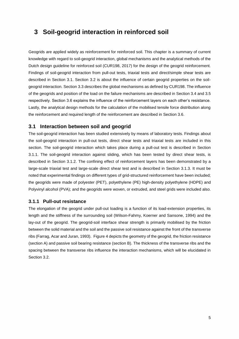
The direct sliding resistance is generally expressed in terms of two contributions. The first contribution
is related to the shear resistance mobilised at soil-solid grid surface areas. The second contribution is
related to the shear resistance mobilised at soil-soil interface (Moraci et al, 2014). The interface
coefficient of direct sliding (𝑓𝑑𝑠) is the ratio of the interface shear strength relative to the soil internal
shear strength. Equation 3.1 defines 𝑓𝑑𝑠 as a function of the fraction of solid geogrid surface area that
is in contact with the soil (𝛼𝑑𝑠), the soil-geogrid skin friction angle (𝛿) and the soil friction angle in direct
shear (𝜑𝑑𝑠).
𝑓𝑑𝑠 = 1 − 𝛼𝑑𝑠(1 −𝑡𝑎𝑛𝛿
𝑡𝑎𝑛𝜑𝑑𝑠) (3.1)
Figure 5 depicts the dependency of 𝑓𝑑𝑠 on the relative aperture size with respect to the soil particle size
(𝛼𝑑𝑠). The soil types (silt, fine sand, sand, gravel and cobbles) in Figure 5 are just used as example; 𝛼𝑑𝑠
will depend on both the grain size and the aperture size of the geogrid. For silt, 𝛼𝑑𝑠 = 𝛼𝑠, which means
that the total geogrid surface area is in contact with the soil. In case of a slightly larger particle size than
silt (fine sand and sand), the direct shear resistance is partly mobilised by geogrid-soil interface friction
and partly by soil-soil interface friction. In case of a slightly larger particle size than sand, the soil particle
size turns out to be similar to the grid aperture size. The shear zone is located at a certain distance from
the geogrid, defining the shear resistance by soil-soil interface friction. In case of cobbles, the particle
size has become too large to penetrate the geogrid apertures. The contact between themselves and the
surface grid surface leads to a value of 1 for 𝛼𝑑𝑠. The interface shear strength will be a factor 𝑡𝑎𝑛𝛿
𝑡𝑎𝑛𝜑𝑑𝑠
lower than the soil internal shear strength (Jewell, Milligan, Sarsby and Dubois, 1984).
Figure 5: Visualisation of the dependency of the interface coefficient of direct sliding on the relative aperture size of the geogrid with respect to the particle size (Jewell et al, 1984).

8
3.1.3 Increase of confining pressure
The influence of the geogrids on the confining effect has been demonstrated (Ruiken and Ziegler, 2008)
using a large-scale triaxial test of 1.5-meter height and 0.5 meter diameter. Figure 6 shows the effect
that geogrids have on the deformation of the specimen in a triaxial test. It can be noticed that the lateral
deformation is reduced due to the reinforcement. Ruiken and Ziegler (2008) found that the effect of the
reinforcements is similar to an additional confining pressure ∆𝜎3 acting homogeneously over the whole
height of the specimen if the vertical spacing between the geogrids is small enough. The magnitude of
∆𝜎3 depends on the degree of activation (Ruiken and Ziegler, 2008).
Figure 6: Confining effect of geogrids. a) unreinforced specimen b)reinforced specimen (Ruiken and Ziegler, 2008).
The vertical force compresses the soil, which wants to deform laterally. Shear stresses are mobilised
due to the relative displacement between the soil and geogrids. The shear stresses result into the
mobilisation of tensile forces in the geogrid due to confined extension. These tensile forces increase the
confining pressure. As a result, the resistance of the soil against shearing is increased. The risk of failure
will be defined by the maximum mobilised tensile force along the geogrid and/or the tensile strength of
the geogrid (CUR198, 2017).
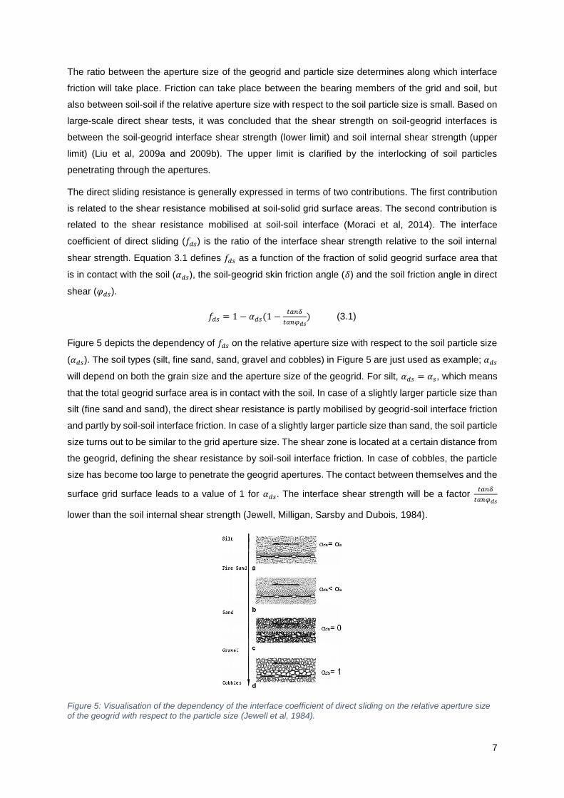
Lees (2014) investigated the confining effect of geogrids by means of large-scale direct shear tests. He
investigated the influence area of one geogrid by varying the vertical distance between the sliding
surface and the geogrid. Direct shear tests were conducted for a one-layer reinforced lightly compacted
well-graded crushed diabase stone with a median diameter (D50) of 5 mm. The confining effect of the
geogrid was considered as a contribution to the cohesion of the soil. Figure 7 shows the results of the
direct shear tests. It was found that the geogrid did not increase the shear strength of the soil when the
vertical spacing was > 30 cm. For a vertical spacing ≤ 20 cm and ≥ 5 cm, the geogrid increased the
measured cohesion of the soil by 4-5 kPa. At a vertical spacing < 1 cm, an apparent reduction of the
soil shear strength was observed.
This confining effect is absent in pull-out test. Confined extension is restrained by the passive resistance
of the soil and particles, which are interlocked between within the apertures by the transverse ribs of the
geogrid (Farrag et al, 1993).
9
Figure 7: Direct shear test results (Lees, 2014).
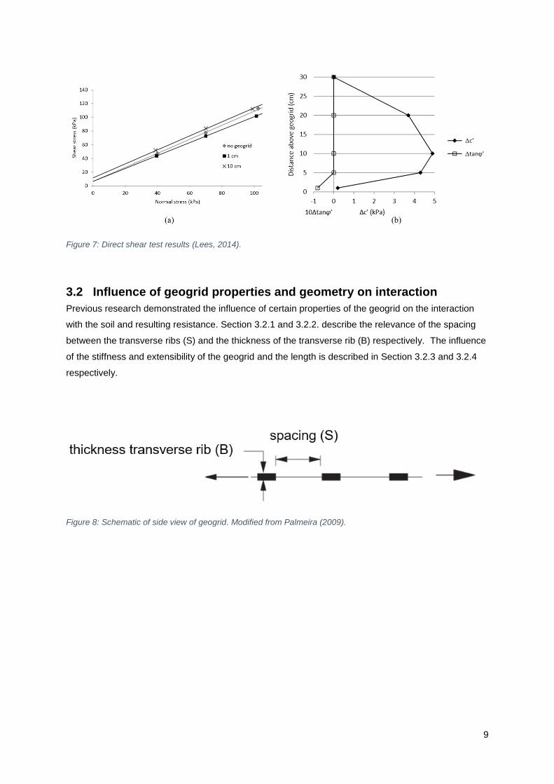
3.2 Influence of geogrid properties and geometry on interaction
Previous research demonstrated the influence of certain properties of the geogrid on the interaction
with the soil and resulting resistance. Section 3.2.1 and 3.2.2. describe the relevance of the spacing
between the transverse ribs (S) and the thickness of the transverse rib (B) respectively. The influence
of the stiffness and extensibility of the geogrid and the length is described in Section 3.2.3 and 3.2.4
respectively.
Figure 8: Schematic of side view of geogrid. Modified from Palmeira (2009).

10
3.2.1 Spacing between transverse ribs
For decreasing spacing between the transverse ribs, the risk that no full bearing resistance can be
mobilised increases. For smaller spacings, larger displacements are required to mobilise a similar
amount of friction and bearing resistance (Wilson-Fahmy et al, 1994).
Palmeira (2009) demonstrated by means of pull-out tests of metal grids at low normal vertical stress (25
kPa) that the passive bearing resistance against the transverse ribs reduces for decreasing spacing
between two consecutive transverse ribs. The passive bearing resistance in front of each transverse rib
cannot exist without a softening region behind the transverse rib. Behind each transverse rib the stress
decreases and forms a disturbed softening region (Cardile et al, 2017). If the spacing between two
consecutive transverse ribs is too small, the softening region behind the transverse rib will affect the
maximum bearing strength developed along the consecutive bearing members (Cardile et al, 2017).
Cardile et al. (2017) found for extruded geogrids that the ratio of the spacing between the bearing
members (S) and the thickness of the transverse ribs (B) must be 𝑆
𝐵> 40 − 50 in order to neglect the
interference phenomena and assume mobilization of maximum pull-out resistance. A lower ratio is
required for smaller particle sizes (Cardile et al, 2017).
3.2.2 Thickness of transverse ribs
The passive bearing resistance will decrease for decreasing thickness of the transverse ribs relative to
the particle size (𝐵
𝐷50). A ratio
𝐵
𝐷50> 7 − 10 is required to avoid interference phenomena as described in
section 3.2.1 (Cardile et al, 2017).
3.2.3 Stiffness and Extensibility
The stiffness of the geogrid depends on the strain level and duration of loading. The stiffness-
dependency on the strain depends on the specific geogrid and the material it is made of. The time-
dependent extension under a constant load (creep) makes that the geogrid behaves less stiff over time
(Watts, 1998). The degree of extensibility4 depends on the stiffness of the geogrid and the soil. Moraci
et al. (2014) and Farrag et al. (1993) concluded from pull-out tests that the extensibility of the
reinforcement has an influence on the peak pull-out strength. The interaction mechanisms in a pull-out
test are characterized by a non-uniform distribution of the shear stresses along the reinforcement, while
uniformly distributed shear stresses are typical for direct shear tests (in case boundary effects can by
neglected). Research has shown that the extensibility of the geogrid only influences the pull-out strength,
not the shear strength against sliding (Farrag et al., 1993). At residual strength, the influence of the
extensibility on the strength is negligible. The effects become especially dominant at relative long
reinforcements and at high confining stresses (Moraci et al, 2014). The more extensible the geogrid, the
more the extensibility affects the shear stress distribution along the geogrid.
4 Inextensible geogrids are defined as those for which the tensile strain in the geogrid is significantly less than the horizontal extension required to develop an active plastic state in the soil. Extensible geogrids are defined as those for which the tensile strain in the geogrid is equal to or larger than the horizontal extension required to develop an active plastic state in the soil (Bonaparte, 1988). It must

11
Figure 9 shows the load-displacement curves between a relatively extensible geogrid and relatively
inextensible geogrid during a pull-out test. The right figures give the approximated percentage of the
frictional resistance and passive soil resistance (bearing resistance) against the transverse ribs for the
extensible and inextensible geogrid (Wilson-Fahmy et al, 1994). It can be observed that both the friction
and passive soil resistance are immediately mobilised for inextensible geogrids, while an increasing
level of strain is required to mobilise the passive soil resistance for increasing extensibility (Wilson-
Fahmy et al, 1994).
Figure 9: Comparison load-displacement curves between a relatively extensible geogrid and relatively inextensible geogrid during a pull-out test. Predicted and measured displacements at different locations along geogrids for a geogrid length of 0.92 m (Wilson-Fahmy et al, 1994).
3.2.4 Length
Wilson-Fahmy performed pull-out tests for geogrid lengths of 0.31 m, 0.92 m and 1.70 m. For the short
geogrids, the total resistance is more or less uniformly shared by all the transverse ribs. For long
geogrids, the resistance mobilises in a more progressive manner and the shear stress distribution will
become non-uniform (Wilson-Fahmy et al, 1994).
be noted that design guidelines specify the definition of inextensible/extensible geogrids in terms of % of strains in the reinforcement at the design load (British Standard BS 8006-1, 2010).

12
3.3 Global stability
The CUR198 (2017) subdivides the global failure mechanisms in two categories: those which apply to
either the external stability or internal stability of the MSE wall. The external failure mechanisms are
described in Section 3.3.1 and the internal failure mechanisms are described in Section 3.3.2.
3.3.1 External stability
The external failure mechanisms for which an MSE wall must be designed are:
• Exceedance of bearing capacity
• Horizontal translation
• Sliding along deep slip surface
Figure 10: External failure mechanisms (CUR198, 2017).
The external failure mechanisms consider the block of reinforced soil as one moving object. In design,
the external stability should proof that:
• the minimum required length of the reinforcement layers is satisfied;
• the minimum required embedment depth is satisfied.
The main difference between sheet pile walls and MSE walls is the embedment depth. For this research,
we assume that the geogrid-anchored SPW has been embedded sufficiently deep such that there is no
risk of failure due to the types of failure mechanisms depicted in Figure 10.
3.3.2 Internal stability
The internal failure mechanisms for which an MSE wall must be designed are:
• Pull-out of geogrid
• Sliding of soil mass above geogrid layer
• Rupture of geogrid due to exceedance of the tensile strength
• Breakage of the connection of geogrid to facing due to exceedance of the tensile strength.
Geogrids will be pulled out if the driving forces require a tensile force in the geogrid which cannot be
provided by the shear resistance of the soil along the geogrid. Either the length of the geogrid(s) is/are
too small and/or the number of geogrids is too low.

13
Soil may slide along the geogrid layer when the resistance provided by the upper geogrid layers is
insufficient to retain the soil mass against sliding. The driving forces are the active horizontal forces
behind the reinforcement.
In practice, when a MSE wall is designed well, exceedance of the tensile strength of the geogrid is
commonly not a limiting factor. This is also concluded from large-scale direct shear tests (Lees, 2014).
Whether and how the geogrid is connected to the facing depends on the type of facing used.
In design, the internal stability check should proof that:
• the minimum required strength of the reinforcement is satisfied;
• the maximum allowable spacing between the reinforcement layer is not exceeded.
Figure 11 gives an overview of the locations within an MSE wall where pull-out failure mechanisms or
sliding mechanisms may occur.
Figure 11: Internal failure mechanisms of MSE walls and corresponding laboratory tests (Moraci et al, 2014).

14
3.4 Influence of geogrids on failure mechanisms
Jacobs, Ruiken and Ziegler (2016) and Ziegler (n.d.) conducted model tests of both unreinforced as
geogrid reinforced soil retaining walls. They studied the development of earth pressures and
distributions, as well as the kinematic behaviour. Tests were conducted for both connected and non-
connected geogrids. A uniformly distributed surcharge load was applied, while the soil was induced to
failure by horizontally pulling the facing away from the soil.
Figure 12 shows the results of the test with 5, 2 and no geogrids. By means of Digital Particle Image
Velocimetry (DPIV) software, the particle rotations have been computed.
Their main findings are:
• The distance between the major failure surfaces and wall facing decreases for increasing
number geogrid layers.
• The lateral earth pressure exerted on the sheet pile wall reduces for increasing number of
geogrid layers.
• No substantial difference was observed between the results of a reinforced soil containing
either connected or non-connected geogrids.
• Soil arching was observed between two geogrid layers at very small facing displacements.
Figure 12: Shear zone development from particle rotations unreinforced and reinforced specimens (Jacobs,
Ruiken and Ziegler, 2016).

15
Figure 13 shows a close up of the geogrid at the facing, in which the left and right figure depict the
horizontal soil displacements and soil particle rotation respectively (Ziegler, n.d.).
The following was observed:
• In contrast to a single slip surface for unreinforced soil, various slip surfaces develop for
reinforced soils.
• Those slip surfaces develop one after the other at the position with the lowest resistance of
the soil.
• The slip surface seems to be orthogonal to the geogrid.
• The soil is confined horizontally at the geogrid.
Figure 13: a) horizontal soil displacement b) soil particle rotation (Ziegler, n.d.).

16
3.5 Influence load position on failure mechanisms
Ahmadi (2020) analysed 1g physical model tests of reinforced soil. Three different types of
reinforcement were tested, among which geogrids. The soil was induced to failure by a strip footing load,
while the wall was allowed to move horizontally. Figure 14 shows the total shear strain results obtained
from DPIV for the test configuration of four geogrid layers and a rigid facing. With regard to the failure
mechanism, the following was concluded:
• Two slip surfaces are formed, which intersect the rigid facing with an angle 45 −𝜑
2 to the
vertical.
• The shallow slip surface initiates at the inner edge of the loading plate.
• The deeper slip surface initiates at the outer edge of the loading plate.
Figure 14: Total maximum strains obtained from DPIV (Ahmadi, 2020).
Ahmadi (2012) performed small-scale physical model tests to investigate the bearing capacity of strip
footing in reinforced sand backfills and flexible retaining walls. The flexible wall was fixed to the bottom
of the test box, while failure was reached by increasing the surcharge load on the strip footing. The
influence of the load position was analysed for the unreinforced case and reinforced case.
For a strip footing positioned > 16.8 cm from the SPW, two spiral failure zones were observed. The
shallow spiral failure zone initiates at the inner edge of the loading plate, while the deeper spiral failure
zone initiates at the outer edge of the loading plate. A plastic area was observed between the two spiral
slip surfaces. A rigid soil body area was observed between the shallow slip surface and wall. For a strip
footing positioned < 7 cm from the SPW, failure completely moved to the walls side.

17
Figure 15: Influence of load position on failure mechanism (Ahmadi and Hajialilue-Bonab, 2012).
a) load positioned 6 cm from SPW b) load position 16.8 cm from SPW c) load position 27 cm from SPW
One of their conclusions was that higher bearing capacity was found for load positions further away from
the wall facing. When the strip footing load is far from the wall facing, a deeper and therefore longer
spiral slip surface developed that started from the outer edge of the loading plate. A deeper slip surface
will cross more reinforcement layers and will intersect deeper soil layers with larger pull-out resistance.
Finally, a larger pull-out resistance and larger moment arm resulted to higher bearing capacity (Ahmadi
and Hajialilue-Bonab, 2012).
3.6 Interaction between geogrid layers
CUR198 emphasizes that no full friction can be mobilised along both sides of the geogrid due to the
interaction between the geogrid layers. As a consequence, the friction along only one side of the geogrid
is considered for the calculation of the maximum mobilised tensile forces along the geogrid (CUR198,
2017).
As mentioned in Section 3.4, Jacobs et al. (2016) observed arching of the soil between the geogrid
layers, which enhanced the confining effect of the geogrid layers (Jacobs et al., 2016).

18
3.7 CUR198: analytical methods for checking the internal stability
This research focusses on the mobilised tensile forces in the geogrid. The CUR198 (page 84) has
included one analytical design-calculation to compute the maximum mobilised tensile force per unit area
of the reinforcement (𝑅𝑎;𝑖). The analytical design-calculation for geogrids covering an area > 50% per
unit meter facing is given by equation 3.2 and 3.3:
𝑅𝑎;𝑖 = (𝜎𝑣,𝑖 ∙ 𝜇𝑝 + 𝑐 ∙ 𝑎𝑏𝑐′ ) ∙
𝐿𝑎,𝑖
𝛾𝜇 (3.2)
𝜇𝑝 = 𝑎′tan(𝜑′) (3.3)
in which:
𝜎𝑣,𝑖 = the design value of the vertical effective pressure acting on reinforcement layer i [kPa],
𝜇𝑝 = the interaction coefficient [-],
𝑐 = the effective cohesion [kPa],
𝑎𝑏𝑐′ = influence factor of the cohesion on the mobilised friction [-]
𝐿𝑎,𝑖 = effective length or anchorage length, which is the length of reinforcement layer i outside the
active soil wedges [m],
𝛾𝜇 = partial factor of the mobilised friction [-],
𝑎′ = influence factor of the internal friction angle on the mobilised friction [-]
𝜑′ = internal friction angle [°].
The influence factors 𝑎𝑏𝑐′ and 𝑎′ have to be determined by laboratory tests (CUR198, 2017). The soil
properties 𝑐 and 𝜑′ are commonly determined by means of triaxial tests, direct shear tests, simple
shear tests or biaxial tests. Commonly, pull-out tests or direct shear tests are performed to determine
the apparent interaction coefficient 𝜇𝑝
𝛾𝜇 (Moraci et al, 2014).
Figure 16 gives the theoretical maximum tensile force distribution along a reinforcement layer. At the
rear end of the reinforcement, the tensile force is zero. Dependent on the frictional force, which can be
mobilised per unit length of the reinforcement, the tensile force will increase along the reinforcement
layer from the rear end to the intersection with the active soil wedge (𝑅𝑎;𝑖;𝑘). The tensile force will be
cut-off at the tensile strength of the reinforcement (𝑅𝑔;𝑖;𝑘). At the connection of the reinforcement layer
with the facing, the mobilised tensile force is reduced to the tensile force in the connection (𝑇𝑐𝑜𝑛𝑛;𝑖;𝑘).
Between the tensile force in the connection (𝑇𝑐𝑜𝑛𝑛;𝑖;𝑘) and the maximum tensile force reached, the
tensile force will increase along the reinforcement layer by the frictional force per unit length. The
tensile force in the connection (𝑇𝑐𝑜𝑛𝑛;𝑖;𝑘) is equal to the mobilised tensile forces in case of a rigid facing

19
(CUR198, 2017).
Figure 16: Analytical design calculation for the tensile force distribution along a reinforcement layer (CUR198 (page 131), 2017).
The required length of the geogrid is defined by the required tensile force (𝑇𝑖) and maximum frictional
force per unit area along the geogrid-layer (𝑅𝑎;𝑖). The maximum mobilised tensile forces must not be
exceeded such that either failure due to (1) pull-out of reinforcement layers or (2) sliding along
reinforcements layers can occur. These two failure mechanisms will be discussed in Section 3.7.1 and
3.7.2.
3.7.1 Local internal stability
Culmann’s active wedges method or the Tie Back wedge method can be used for extensible
reinforcements – such as geogrids – for the computation of the required tensile forces along the geogrids
to prevent pull-out failure mechanisms. We refer the reader to CUR198 for more information regarding
the calculation methods for the required tensile force in the geogrid. We will elaborate on the method
proposed by CUR198 to compute the mobilised tensile force distribution along the geogrid.
Figure 17 shows the schematization of the calculation method for the mobilised tensile force in the
geogrid according to the Tie back wedge method. The important difference between the Tie back wedge
method and Culmann’s active wedges method for the calculation of the mobilised tensile forces is the
assumption of the active zone. The Tie back wedge method assumes a critical slip surface, which cuts
the SPW at the toe with an angle 𝜃𝑎:1 = 45 −𝜑
2 to the vertical. Culmann’s active wedges method also
assumes a straight critical slip surface, but derives the critical angle of the wedge based on a force
equilibrium analysis. For every possible wedge – i.e. the triangular shaped soil mass enclosed by the
SPW and potential critical slip surface – a force equilibrium calculation is conducted in order to find the
wedge, which exerts the highest lateral active soil pressures against the facing of the reinforced soil

20
(specific for horizontal soil surfaces). Note that Culmann’s method can also be applied for non-horizontal
surfaces (more complex geometries).
The total height of the MSE wall is denoted by the capital H and the total length of reinforcement layer i
by the capital Li. It is assumed that reinforcement layer i takes up the active lateral soil pressures of the
soil layer hi acting against the SPW. The tensile force which can be mobilised (Ra;i) is equal to the
maximum mobilised friction along the length of the reinforcement outside the active soil wedge (La;I).
Figure 17: Schematization of the calculation method for the mobilised tensile force in the geogrid according to the Tie back wedge method (CUR198, 2017).

21
3.7.2 Global internal stability
In Section 3.7.1, the required tensile force is calculated for each reinforcement layer separately. Next,
the required tensile force – denoted by 𝑇𝑖 in Figure 18 – against a sliding soil mass must be determined
for each reinforcement layer i by taking into account the reinforcement layers above the particular
reinforcement layer. Here, i is the number of the relevant reinforcement layer where the bottom
reinforcement layer is i = 1. Figure 18 gives the schematization of the Two-Part Wedge method, which
is proposed in CUR198 as design calculation to check whether the design of the reinforcement delivers
sufficient tensile force against sliding soil masses. The reader is referred to (CUR198, 2017) for more
information. The main assumption for the calculation of the maximum mobilised tensile forces – denoted
by R - along the reinforcement are:
• The front active wedge zone ABCD is located within the reinforced soil zone and intersects the
facing with an angle 𝜃1 to the vertical.
• The back active wedge zone DCE exerts active lateral forces against the front active wedge
zone. The back active wedge zone is defined by the angle 𝜃2.
• Tensile force can be transferred to the soil along the part of the reinforcement outside the active
wedge zones.
In case of strip footing loading, the most critical wedges have to be found by iteratively changing both
𝜃1 and 𝜃2.
Figure 18: Two Part Wedge method to check the mobilised anchor forces against a sliding soil mass driven by the active lateral forces behind the reinforcement. Modified from (CUR198, 2017).

22
4 Soil-anchor interaction in sheet piling
Since geogrids have not been included in CUR166 as type of anchorage, and the use of geogrids as
anchors is relatively new, few research is available with regard to the mechanisms involved in the soil-
geogrid behaviour specific for geogrid-anchored SPWs. This fact emphasizes the relevance of this
research. (Detert et al, 2019) and (van Duijnen et al, 2021) are – as far as the author is aware – the first
research studying this type of SPW-anchorage. Section 4.1 describes the interaction between soil and
(geogrid) -anchor. Section 4.2 gives an overview of the failure mechanisms for which an anchored SPW
must be designed for. Section 4.3 describes the analytical design calculation, which is proposed in
CUR166 for the calculation of the required anchor length for conventional anchors. This analytical design
calculation, known as Kranz’s method, was already mentioned in Chapter 1.
4.1 Interaction soil-anchor
4.1.1 Membrane effect
The downdrag forces that arise from soil settlement relative to the retaining wall have been studied for
steel-reinforced soil walls (Damians et al, 2013). Because the backfill soil settled more than the concrete
facing, frictional forces developed at the interface soil-wall. Additionally, vertical pressure is transferred
to the concrete facing – which is build up out of stacked concrete panels - because of backfill soil that
hangs-up on the connections between the panel units and reinforcement (Damians et al, 2013).
Similar behaviour can be expected at the connection of the geogrid to the SPW. Due to the surcharge
load, soil is pushed downward and will likely drag along the geogrid-anchor. As a result, vertical soil
pressures may reduce due to the friction between the geogrid-soil. The friction mobilises tensile forces
in the geogrid. The vertical components will be transferred via the connection to the SPW.
Figure 19: Transfer of vertical soil pressures to the retaining wall (Damians et al, 2013).

23
4.1.2 Interaction between geogrid-anchors
Van Duijnen et al. (2021) presented and simulated one of the geogrid-anchored SPWs of Windpark
Krammer (see Chapter 2), using a 2D Finite Element Method (FEM) program (Plaxis bv., 2019).
One of the interesting findings concerned the interaction between the three geogrid-anchors. It was
found that the upper two anchors only transfer their load along their part that is located behind the
rear end of the underlying anchors. The bottom anchor transfers its force to the soil outside the
active wedge alike the analytical design calculations for reinforced soils.
Figure 20: Proposed for design of geogrid-anchorage: the effective length of an geogrid-anchor as a function of the underlying anchor lengths (van Duijnen et al, 2021).
4.1.3 Soil-geogrid interaction for double layered anchor
As depicted in Figure 3 of Chapter 2, the anchors consisted of a geogrid, which was wrapped around a
hinged connection. Van Duijnen et al. (2021) studied the tensile force distribution and mobilised frictional
forces along the top and bottom geogrid layer of one anchor. The following was found:
• The largest share of the anchor force was mobilised by the friction along the bottom of the
bottom geogrid, around 80%.
• The bottom of the top geogrid and top of the bottom geogrid show equal frictional force
distributions along the geogrid. A very small share of the anchor force was provided by these
two inner interfaces.
• Part of the total friction was mobilised in the active zone, i.e. the zone enclosed by the SPW and
the critical slip surface. Hereby, the critical slip surface is assumed to cut the SPW at the point
of zero shear forces with an angle equal to 45 −𝜑
2 according to Mohr Coulomb’s theorem.

24
4.2 Global mechanisms
Since we want to simulate failure due to exceedance of the anchor forces in our experiments, other
failure mechanisms for which an SPW must be designed are prevented from happening. The following
failure mechanisms are prevented:
• Loss of stability due to shearing along a circular slide surface
• Plastic failure of the SPW
• Exceedance of the vertical bearing capacity
• Piping
• Tensile failure of the geogrid anchorage
These failure mechanisms were prevented by (1) testing dry soil, (2) only modelling the upper part of
the SPW, (3) using a very rigid SPW and (4) a geogrid with sufficient high tensile strength.
The only failure mechanisms considered are:
• Failure due to shearing along a deep straight slide surface,
• Exceedance of the passive earth pressure.
Since the free length of the SPW is generally a fixed parameter, exceedance of the passive earth
pressure will be linked to exceedance of the anchor forces. The geogrid-anchorage can increase the
resistance against bending and translation by increasing the number of anchor points and length of the
geogrids.
The analytical calculation method used to verify whether the length of the anchors is sufficient in order
to prevent this type of failure is described in the next section.
Figure 21: Failure mechanisms which must be checked for the design of a sheet pile wall (CUR166, 2008). a) Kranz’s deep sliding surface b) Bishop’s deep circular sliding surface c) instability due to piping

25
4.3 CUR166: analytical methods to determine the required length of conventional anchors
Since no analytical design method exists for the required length of the geogrid-anchorage, the analytical
method used to calculate the required length of conventional anchors is described shortly. Kranz’s
method is the analytical method which describes the deep failure mechanism as a consequence of a
too short anchorage design.
Kranz’s method is based on a force equilibrium calculation. Active soil forces according to Rankine are
assumed to act along the SPW and the active zone is defined by the slip surface as defined by Mohr
Coulomb. Accordingly, the active soil wedge ABA’ in Figure 22a intersects the SPW at an angle 45 −𝜑
2
to the vertical. A deep sliding surface is assumed between the point of zero shear forces in the SPW
and the tip of the anchor wall. Additional active soil forces will act behind the anchor wall for which also
wedge – as defined by Mohr Coulomb -is considered. The sliding surface and active soil wedges
surround the zone of soil from which the anchor acquires soil support.
For an anchor wall, the mobilised anchor force is defined by the passive bearing resistance of the soil
in between the active soil wedge and the anchor wall. The required length can be directly derived from
Kranz’s method. In case of grout anchors, the mobilised tensile force is based on empirical relations.
The deep sliding surface intersects the SPW at the point of zero shear forces and cuts the grout anchor
halfway (line BC in Figure 22b). The shear stress distribution of grout anchors is approximately known
(Figure 22c). However, no analytical design calculation has been formulated yet. The length of the grout
body must be sufficient such that no failure along Kranz’s deep sliding surface will occur. The friction
along the second half of the grout anchor and the soil resistance along the deep sliding surface must
not be exceeded by the active earth forces against the SPW.
Figure 22: Kranz’s stability method to calculate the required length of (a) an anchor wall and (b) a grout anchor in order to prevent failure along a deep sliding surface. c) shear stress distribution along a mono or duplex grout anchor (CUR166, 2008).

26
5 Comparison numerical modelling of geogrids and
measurements in literature
This chapter evaluates the similarities between numerical and field/experimental measurements of
previous studies in Section 5.1. Accordingly, it is evaluated to what extent the geogrid modelling method
influences the numerical results and what factors must be considered for the choice of geogrid modelling
method in the numerical model of the 1g small-scale experiment of the geogrid-anchored SPW. The
conventional method models the geogrid as a tensile membrane with either a strain-dependent or
constant tensile stiffness. In Section 5.2, a new geogrid modelling method is proposed to include the
confining effect. Section 5.3 evaluates the findings from literature and their relevance in the numerical
modelling of a geogrid-anchored SPW.
5.1 Comparison numerical results and experimental-field measurements
Several studies validate results of numerical models of geogrid-reinforced soils with field or experimental
measurements. Hatami and Bathurst (2005) and Ahmadi (2020) analysed numerical models of MSE
walls and compared the results with measurements during large-scale and small-scale test. The
outcome is summarized shortly in Section 5.1.1. Other studies analysed numerical models of MSE walls
and compared the results with measurements during and after construction of full-scale MSE walls
(Araújo, Palmeira and Macêdo, 2012) (van Duijnen, Linthof, Brok and van Eekelen, 2012). These
findings are described in Section 5.1.2.
5.1.1 Simulation of large and small-scale 1g physical models of MSE walls
Hatami and Bathurst (2005) performed three well-instrumented, large-scale 3.6 m high test walls. The
wall had a modular block (segmental) facing and a back fill reinforced by either four or six polypropylene
(PP) geogrids or polyester (PET) geogrids. The length of the geogrids were 0.7 times the height of the
wall (in agreement with the design guideline of the National Concrete Masonry Association (NCMA) and
American Association of State Highway and Transportation (AASHTO, 2002 version). The backfill sand
was uniformly sized and had a median diameter (D50) of 0.34 mm. A 2D numerical model for the
reinforced soil test walls was developed and validated against measurements of, among others, the
deformation of the modular block facing. Measurements were performed up to the end of construction
i.e. the operational condition or serviceability limit state. For the numerical model, the finite-difference-
based program FLAC was utilized. In this numerical model, the geogrid was modelled by two-noded
elastic-plastic cable elements with a strain-dependent tangent stiffness and a tensile yield strength and
no compressive strength. The geogrids were rigidly connected to the back of the facing blocks through
beam elements with a large axial stiffness value. The program FLAC includes a pre-defined cable grout
utility to model the geogrid-soil interaction. Since no pull-out behaviour was observed in the test, Hatami
and Bathurst (2005) did not activate this feature and consequently modelled the interface as fully rough
i.e. geogrid and soil displace as one object. The numerical results during and at the end of construction
were shown to be in good agreement generally with, among others, the wall deformation and
27
reinforcement strains. Since this types of geogrid are known for its non-linear stress-strain response
with time and strain level, the magnitude of the stiffness of CRS5 tests was reduced, to match the
stiffness for longer duration constant load (creep) tests in order to take into account of the duration of
the construction stage. Moreover, the CRS tests were carried out at low strain rates in accordance with
strain rates in the field. The shape of the load-strain curve was used to determine the initial stiffness and
strain-softening coefficient of the strain-dependent tensile stiffness function of the geogrid.
Ahmadi (2020) conducted small-scale 1g physical model experiments for a MSE wall, which was
subjected to strip footing loading. Experiments were performed with either a rigid (concrete) or flexible
(wood) wall facing. A poorly graded dry sand with no fines and a median diameter (D50) of ~1.64 mm
and a relative density of 88% was used as backfill. For both types of wall, an experiment was conducted
with either four or eight reinforcement layers, which were connected to the facing. Different types of
reinforcement were used including a polypropylene (PP) biaxial geogrid. The finite-element program 2D
PLAXIS (Brinkgreve et al, 2004) was used to model the MSE wall. The geogrid was modelled as a 1D
tensile element with stiffness equal to the short-term stiffness (<4% strain) of 150 kN/m. The geogrid-
soil interaction was modelled by an interface with a reduction factor of 1, which means that the interface
was not activated and a fully rough interface was assumed.
Ahmadi (2020) found around 10% difference in lateral wall deflection between the experimental and
numerical results. The numerical and test result were considered to agree well.
Besides the small-scale 1g physical model experiments of an MSE wall, Ahmadi (2020) analysed large-
scale 1g physical model experiments of an MSE wall also. A poorly graded sand with a median diameter
(D50) of ~1.2 mm and relative density of 95.8% was used as backfill. The moisture content was 12.4%.
A polyester (PET) geogrid was used as reinforcement. The reinforcement consisted of eight layers of
geogrids. The experimental results were compared with a 2D PLAXIS model in which the geogrids were
modelled as 1D tensile elements with a stiffness equal to the long term (100 hours) stiffness of (<0.5%
strain level) of 670 kN/m. The soil-geogrid interaction was modelled by a reduction factor on the soil
shear strength equal to 1. A strip footing load of 300 kPa was applied to the soil. This loading plate was
free to move horizontally.
Figure 23 shows the results of the measured and numerically computed maximum tensile force in each
geogrid layer for the rigid facing and flexible facing after applying a strip footing load of 300 kPa.
Numerical results were computed for a model in which the loading plate was restricted to move laterally
(PLAXIS 2D-Restricted) and free to move laterally (PLAXIS 2D -Free). The latter corresponds better
with the experiment as the footing was not restricted during testing.
5 CRS tests are Constant Rate of Strain tests

28
Figure 23: Measured and numerically computed maximum tensile force in each reinforcement layer after applying the strip footing load of 300 kPa. The upper figure (a) gives the test measurements and numerical results (PLAXIS) for the test configuration with a rigid facing and the lower figure (b) gives the results for the test configuration with flexible facing (Ahmadi, 2020).
Comparison of the test results and numerical results of Figure 23 showed a difference of 52% to 62%
for the sum of the maximum tensile forces in the reinforcement layers and the maximum wall deflection
(Ahmadi, 2020). However, good agreement between the numerical and test results was achieved when
the compaction process of the preparation procedure of the experiment was simulated in the numerical
model by including the dynamic compaction load. Figure 24 and Figure 25 show the results of the lateral
wall deflection and tensile force distribution along the second geogrid layer after simulating the dynamic
compaction load first, and secondly applying a strip footing load of 300 kPa. The maximum tensile force
is located under the center of the loading plate in the test results, while the maximum tensile force is
located close to the wall face in the numerical results. The magnitude of the maximum tensile force
agrees well between the test and numerical results. It was found that the movement of the wall at that
location will be the same, when the area under the tensile force distribution curve for the test and
numerical results are the same.

29
Figure 24: Lateral wall deflection after applying the strip footing load of 300 kPa. The dynamic compaction load was simulated prior to strip footing loading (Ahmadi, 2020).
Figure 25: Tensile force distribution along the second geogrid layer, which is located at a vertical distance of 0.75 m from surface level (3/16th the height of the wall). The strain gauges measurements were converted to a tensile force by considering the long-term stiffness of 670 kN/m at 0.5% strain (Ahmadi, 2020).

30
5.1.2 Simulation of full-scale MSE walls
(Perkins, 1999). Araújo, Palmeira and Macêdo (2012) analysed and compared the numerical results
with the measured excess pore pressures, vertical and horizontal displacements during the construction
of one of the MSE walls including an abutment on soft soils for the duplication of a highway in Brazil.
Figure 26 shows a cross-section of one of the abutments studied along its longitudinal direction.
Figure 26: Schematisation of reinforced abutment on soft soils for the duplication of a highway in Brazil (Araújo et al, 2012).
Eight layers of uniaxial geogrid were used to strengthen the abutment. The reinforced abutment
consisted of a soil body of coarse sand. The finite-element program PLAXIS was used for the 2D
numerical modelling of the reinforced embankment. 1D tensile elements were used to model the
geogrids and the soil-geogrid interaction is modelled by using a reduction factor, Rint of 0.9 to the friction
shear strength of the soil. Araújo et al. (2012) found that the vertical displacements and maximum
excess pore pressures computed by the numerical model agreed well with the measured values in the
field. However, the horizontal displacements were significantly overestimated by the numerical model.
Araújo et al. (2012) gave several possible explanations, such as the influences of 3D conditions which
were not simulated and the rate of dissipation of excess pore pressures was faster in the numerical
model.
Similar significant deviations in lateral displacements were also found in other studies, that analysed
reinforced retaining walls or embankments on soft soils numerically. An example is simulated of a 10 m
high MSE wall reported by van Duijnen et al. (2012). The numerical model had overestimated the
deformations of the wall, because the reinforced fill and the interaction between the geogrid and soil
behaved stiffer in reality (van Duijnen et al. 2012).

31
5.2 Alternative 2D modelling of geogrid
Lees and Clausen (2019) proposed a new method, called the ‘c’ profile method’, to model the geogrid
for reinforced soils. They argued that the mechanism called ‘stabilisation’, which we refer to as the
confining effect, is not captured in conventional methods of geogrid modelling. Based on large scale
triaxial compression tests results and plate load tests, the discrepancy between the measured and
modelled stress-strain response has been captured (Lees, 2014). The conventional geogrid modelling
method describes the geogrid by a 1D tensile element (2D) and assigns a tensile stiffness (either strain
dependent or not) to the element, which is generally determined from CRS testing. When the geogrid is
modelled according to the conventional method (1D tensile element), the increase in soil strength of the
soil at a larger distance from the geogrid is not taken into account (Lees, 2014). The c’ profile method
includes a non-linear failure envelope as depicted in Figure 27. The maximum of the failure envelope is
found at the elevation of the horizontal geogrid surface and the minimum is found outside the zone of
influence. The slope k represents the inter-particle frictional components of strength. The zone of
influence depends on the degree of inter-particle interlock, which is likely to increase for increasing grain
size. The c’ profile method was implemented in PLAXIS 2D within a constitutive model called ‘Stabilised
Soil (SS) model’. This SS model is a linear elastic and perfect plastic (LEPP) model having associated
plasticity in non-stabilised soil while increasing non-associativity in stabilized soil (Lees and Clausen,
2019).
Figure 27: Non-linear failure envelope of c’ profile method (Lees and Clausen, 2019).
Figure 28a and b show the results of triaxial compression tests and plate load test results for the
measured (laboratory) and numerically calculated deformation using either the conventional method
(modelling the geogrid as 1D tensile element) or the newly proposed method (c’ profile method). The
former method is labelled as ‘FEA geogrid element’ and the latter method is labelled as ‘FEA c’ profile’
in Figure 28a and b. For the triaxial compression test, a well-graded sandy gravel compacted to 98%
proctor density was used (Lees, 2014). One polypropylene welded geogrid was incorporated in the soil.
For the plate load tests a 0.3 m thick granular sub-base stabilized with geogrid overlying a 0.9 m thick
sand subgrade was prepared. Two layers of Tensar TX180 geogrids were placed; one at 0.15 m depth
and one at the top of the subgrade. The results of the finite element analyses (FEA) correspond well
with the measured strains in Figure 28a and the load-displacement curve in Figure 28b for the

32
unreinforced case. For the reinforced case, the results of the conventional modelling method (FEA
geogrid element) significantly overestimate the radial strains in Figure 28a and vertical displacements
in Figure 28b. Much better agreement is found between the measurements and numerical results if the
c’ profile method is used.
Figure 28: (a) Triaxial compression test results and numerical results (PLAXIS, denoted as ‘FEA’) (b) Plate load test results and numerical results (PLAXIS, denoted as ‘FEA’). Results are given for the reinforced and unreinforced case. FEA c’ profile represents the numerical results obtained from the SS model. FEA geogrid element are the results obtained from the Hardening Soil model and the geogrid modelled as a tensile membrane (conventional geogrid modelling method) (Lees, 2014).
Additionally, Lees and Clausen (2019) conducted full-scale granular platform loading tests on a soft clay
subgrade. Figure 29a shows the full-scale stabilized platform loading test. Three layers of multi-axial
polypropylene (PP) geogrid were placed in a 1.1m thick well-graded sand and gravel of crushed rock.
The measurements were compared with the results of the SS model and the LEPP Mohr-Coulomb
model with the geogrid modelled according to the conventional method. Figure 29b shows the load as
a function of the settlement for the field measurements (‘Measured’), the results of the 2D PLAXIS model
using the SS model (‘FEA SS model’) and the results of the 2D PLAXIS model using the conventional
method (‘FEA memb.el.’). For clarity, the FEA SS model is a soil model based on the c’ profile method.
The FEA mem. el. model includes the geogrids as 1D tensile elements. The SS model predicts the
failure load well, while the LEPP Mohr-Coulomb model with membrane elements (conventional method)
underestimates the failure load.

33
Figure 29: a) Schematisation of platform loading test b) Applied pressure against measured and numerically computed settlement. Numerical results are given for the SS model and the Soil Hardening model with a tensile
membrane incorporated (conventional method) (Lees and Clausen, 2019).
5.3 Limitations of the 2D geogrid modelling in this study
In our study, the small-scale 1g physical model has been simulated using a 2D finite element model for
which the finite-element program PLAXIS 2D is utilized. In a plane strain (2D) finite element model, the
typical grid-structured geometry of the geogrid cannot be modelled. PLAXIS 2D (Plaxis bv., 2019)
models the geogrid with a special geogrid tensile line (1D) element. The behaviour of these geogrid
elements is described by an elastic normal axial stiffness (EA) and optional a maximum tensile force at
which rupture occurs i.e. the tensile strength. The bending stiffness and compression stiffness are zero.
Interfaces has been used along the geogrid in order to simulate the shear band between the soil and
geogrid. Through interface friction the geogrid can transmit load to the surrounding soil or vice versa.
This shear band can be described by a reduction factor, 𝑅𝑖𝑛𝑡, which has been applied to the soil shear
strength. Another option is to define a dummy soil material for this interface.
Referring to Chapter 3 in which the soil-geogrid interaction is described, the following limitations can be
listed when modelling the geogrid as a 1D tensile element with an elastic axial tensile stiffness:
1. Strain level dependency of geogrid stiffness is not included.
2. The time dependency of geogrid stiffness (creep) is not taken into account.
3. The effect of particle interlocking on the vertical distance above and below the geogrid (zone of
influence) at which the confining effect increases the soil shear strength.
4. The non-linear increase of pull-out resistance at increasing pull-out displacement due to the
extensibility of the geogrid.
5. 3D conditions are not incorporated in the numerical model such as possible tensile strains along
the geogrid in in-plane direction.
The first point would become relevant to include in the numerical model if tensile strain levels in the
geogrid larger than the elastic range are reached. Generally, the tensile stiffness reduces non-linearly
for increasing strain level.

34
The second point needs to be included in the numerical model if the numerical model must simulate the
duration of the construction stage in practice correctly.
The third point is of interest in the numerical model if confining effects play a dominant role. Some of the
previous studies (Hatami and Bathurst, 2005) (Ahmadi, 2020) showed that the numerical results of the
MSE walls agreed reasonable well, whereas others (Araújo, Palmeira and Macêdo, 2012) (van Duijnen,
Linthof, Brok and van Eekelen, 2012) found that the deformations were overestimated by the numerical
calculations. In these models, the geogrids were modelled using the conventional method i.e. as a
tensile membrane. Lees and Clausen (2019) showed that the exclusion of the confining effect in the
numerical model result to underestimated performance of the geogrids when used for stabilized
platforms. The numerical model might under-predict the performance of geogrid reinforcement. When
inter-particle interlock plays a significant role, the use of the conventional geogrid modelling method
must be reconsidered.
The fourth point would become relevant if significant pull-out displacements must be simulated by the
numerical model.
The fifth point is not relevant in this research as only the behaviour of the geogrid-anchor normal to the
SPW is relevant. Modelling the geogrid-anchored SPW under plane strain conditions is allowed,
because identical behaviour can be assumed in in-plane direction.
Concludingly, the first and fourth point will very likely play a role and must be considered carefully when
analysing the numerical results. Experimental results must confirm that the confining effect does not
play a significant role when geogrids are used as anchorage for SPWs. If the confining effect is a
dominant interaction mechanism, point 3 becomes relevant and the way the geogrid is modelled must
be reconsidered.
35
6 Small-scale 1g physical model
This chapter describes the purpose of the small-scale 1g experiments and explains the test set-up in
detail in Section 6.1. Furthermore, it describes how the experiments have been conducted in Section
6.2. Finally, Section 6.3 lists the preparation procedure for each test.
6.1 Experimental set-up
Small-scale 1g experiments have been carried out to measure the soil displacements, sheet pile wall
displacement and corresponding surface loads. The soil displacements and strain in the geogrid were
computed by means of Digital Particle Image Velocimetry (DPIV).
6.1.1 General test set-up
This research focusses on failure of the SPW due to a poor design of the geogrid-anchorage.
Therefore, the only failure mechanisms that are considered is failure due to:
• Pull-out of the anchorage.
• Exceedance of the passive bearing capacity of the soil.
While the free length of the SPW - and accordingly the passive bearing capacity of the soil - is considered
as a constant parameter, the second failure mechanism can be considered as exceedance of the anchor
forces against bending of the SPW.
Figure 30 shows the test set-up of the small-scale 1g model of a geogrid-anchored sheet pile wall. The
test box is made of acrylate and the width, height and length of the box are 10 cm, 30 cm and 52.5 cm.
Plane strain conditions, i.e. 휀𝑧𝑧 = 0 (in-plane direction), are pursued. The sidewalls are lubricated and a
silicone sheet is placed between the lubricated sidewalls and sand in order to reduce the sidewall
friction. For the lubrication a water-based lubricant6 turned out to be the best option after examining the
friction coefficient and transparency of several substances as explained in Appendix A.1
6 The water-based lubricant consists of a water content of 85%. Additionally, glycerin (C3H8O3) and other chemical additives among which hydroxyethylcellulose, citric acid, sodium benzoate, potassium sorbate, pentylene glycol, sorbitol, sodium lactate, urea, lactic acid, serine sodium hydroxide, sodium chloride and allantoin.

36
Figure 30: Experimental set-up
Modelling only the upper part of the SPW in the small-scale physical model was considered sufficient to
investigate these failure mechanisms. Only the top 5 cm of the total embedment is modelled. As a result,
the second failure mechanism will be simulated by the sliding of the SPW along the bottom of the test
box.
The SPW was brought to failure by a surface load. A surcharge load was preferred above a pulling force
– as was applied in the experiments of Kranz (1953) to study the required length of a grout anchor –
because a more realistic failure mechanism could be simulated.
As a matter of perspective, the physical model is related to the shortest SPW installed for Krammer
park. Relating the physical model to the shortest SPW installed for Krammer park, a scale factor of 1:21
is determined based on the free length of the SPW. The SPW in Krammer park had a total length of
8.7 m of which the embedment depth and the free length is around 3.6 m and 5.1 m respectively. Hence,
30% of the total embedment depth is modelled. The SPW type installed was a AZ13-700 with a flexural
rigidity (EI) of 43134 kNm2m-1 (Spingher, 2018). When comparing the depth of the geogrid layers
between the model and the ‘prototype’, the top and third geogrid layer of the thee layered geogrid-
anchorage are incorporated in the 1g physical model. The top and third geogrid layer are ~17.5 meter
and ~7 meter. Accordingly only 22% of the top geogrid and 33% of the third geogrid layer is modelled.
The length of the geogrid-anchorage is reduced in the model as failure must be reached at the maximum
surcharge load which can be applied in the test set-up. The flexural rigidity of the SPW in the physical
model is over-dimensioned7 by a factor of ~6.5 if we assume that the soil (more specifically the stiffness
of the soil) is identical.
7 When one pursues a correct scaled version of the SPW bending deformations, the flexural rigidity of the SPW in the physical
model (𝐸𝐼𝑚𝑜𝑑𝑒𝑙) must be equal to: 𝐸𝐼𝑚𝑜𝑑𝑒𝑙 =1
𝜆3+𝑚𝐸𝐼𝑝𝑟𝑜𝑡𝑜𝑡𝑦𝑝𝑒 (Wood, 2004) Here, 𝜆 is the scaling factor of the length which is
equal to 21, and m is a power law coefficient which describes the stress-dependency of the stiffness of the soil. From triaxial tests, the value for m is determined to be 0.54.

37
6.1.2 Geogrid properties
The geogrids used in the experiment were of the category ‘coated yarn’, textiles of polypropylene
polymers of which the grid structure is formed by intertwining the transverse (weft) and longitudinal
(warp) bundles of fibres. In Figure 31, the geogrid is depicted. The thickness of the transverse ribs is
approximately 0.3 mm and the aperture size is approximately 3-4 mm. The stiffness and strength
properties are derived from grid-tensile tests (Kloster, 2016). The tensile strength is 16.18 kN/m at a
maximum strain of 13.48%. The short-term stiffness at 2%, 3% and 5% axial strain is 191 kN/m, 161
kN/m and 126 kN/m respectively.
Figure 31: Geogrid connected to SPW (left) and close-up of geogrid
6.1.3 Soil properties
Because geogrid-anchored SPWs are applied for sand fills behind an SPW, the logical choice is to use
sand in the experiment as backfill. It was tried to get an interaction between geogrid and soil which is
not influenced by incorrect scaling of the geometrical parameters. According to Cardile et al. (2017),
who analysed the influence of the geometrical relations between sand particle diameters and extruded
geogrids on the interaction mechanisms, the following conditions must be met (Cardile et al, 2017):
• a minimum ratio of the aperture size relative to the thickness of the transverse rib (𝑆
𝐵) of 40 - 50,
• a minimum ratio of the thickness of the transverse rib relative to the particle diameter (𝐵
𝐷50) of
7-10.
Here, the spacing between the transverse ribs and the thickness of the transverse ribs is denoted by S
and B respectively (see also Figure 4). Figure 32 shows the grain particle size distribution of the four
types of sand, which were readily available at the Deltares laboratory facilities. Assuming that Cardile’s
findings also hold for the geogrids used here, the sand with the smallest sand particles available was
chosen to increase the ratio of the transverse rib thickness to the particle diameter (𝐵
𝐷50) up to
approximately 2.2. The sand used for the experiment was Baskarp B15. Baskarp B15 is a poorly graded
sand with a median particle diameter (D50) of 0.137 mm. During the experiment, the sand was densified
to a relative density of around 70%. Preparation inaccuracies are estimated to lead to an error marge of
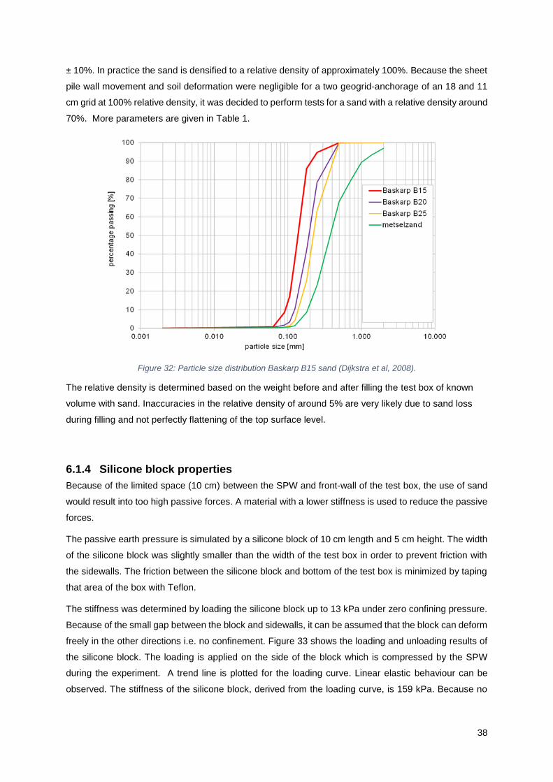
38
± 10%. In practice the sand is densified to a relative density of approximately 100%. Because the sheet
pile wall movement and soil deformation were negligible for a two geogrid-anchorage of an 18 and 11
cm grid at 100% relative density, it was decided to perform tests for a sand with a relative density around
70%. More parameters are given in Table 1.
Figure 32: Particle size distribution Baskarp B15 sand (Dijkstra et al, 2008).
The relative density is determined based on the weight before and after filling the test box of known
volume with sand. Inaccuracies in the relative density of around 5% are very likely due to sand loss
during filling and not perfectly flattening of the top surface level.
6.1.4 Silicone block properties
Because of the limited space (10 cm) between the SPW and front-wall of the test box, the use of sand
would result into too high passive forces. A material with a lower stiffness is used to reduce the passive
forces.
The passive earth pressure is simulated by a silicone block of 10 cm length and 5 cm height. The width
of the silicone block was slightly smaller than the width of the test box in order to prevent friction with
the sidewalls. The friction between the silicone block and bottom of the test box is minimized by taping
that area of the box with Teflon.
The stiffness was determined by loading the silicone block up to 13 kPa under zero confining pressure.
Because of the small gap between the block and sidewalls, it can be assumed that the block can deform
freely in the other directions i.e. no confinement. Figure 33 shows the loading and unloading results of
the silicone block. The loading is applied on the side of the block which is compressed by the SPW
during the experiment. A trend line is plotted for the loading curve. Linear elastic behaviour can be
observed. The stiffness of the silicone block, derived from the loading curve, is 159 kPa. Because no
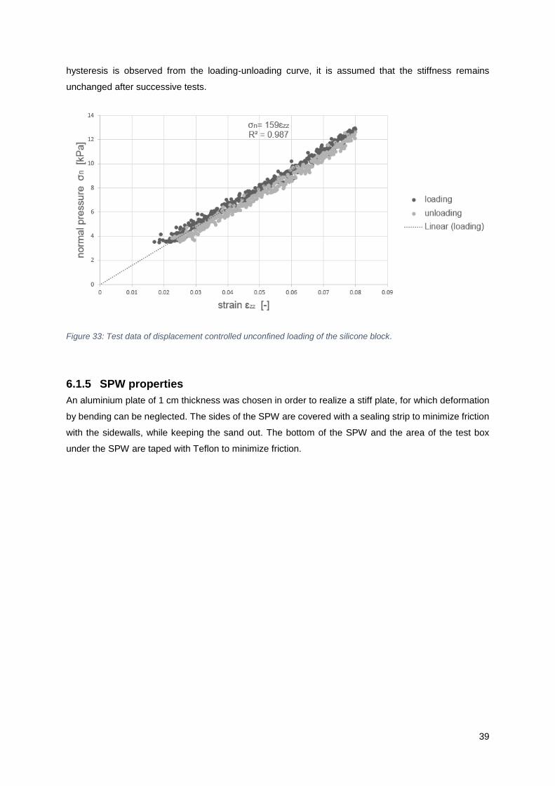
39
hysteresis is observed from the loading-unloading curve, it is assumed that the stiffness remains
unchanged after successive tests.
Figure 33: Test data of displacement controlled unconfined loading of the silicone block.
6.1.5 SPW properties
An aluminium plate of 1 cm thickness was chosen in order to realize a stiff plate, for which deformation
by bending can be neglected. The sides of the SPW are covered with a sealing strip to minimize friction
with the sidewalls, while keeping the sand out. The bottom of the SPW and the area of the test box
under the SPW are taped with Teflon to minimize friction.

40
6.1.6 Footing of surface load
Figure 34 gives a close-up of the footing and surcharge load. The square footing is 10 cm x 9 cm long
x wide and the thickness is 1.5 cm. The footing is made from acrylate. An additional identical footing
plate was placed on top of the bottom footing and a rod was placed in between in order to allow for
horizontal movement of the surcharge load under soil movement. A guidance frame is used to ensure
that a vertical force is transferred to the lower footing plate. A bucket is placed on top of the guidance
frame in which water is pumped to increase the load. The maximum load the test box can sustain is 65-
70 kg. Since we assume plane strain conditions and compare the experimental results with a 2D PLAXIS
model, the load levels are expressed in a force per unit meter. Accordingly, a surcharge load of 70 kg
applied on a footing of 9 cm width is equal to ~7.6 kN/m.
Figure 34: Close-up of top load

41
6.1.7 Summary of properties used
Table 1-5 summarizes all relevant properties of the sand, sheet pile wall, geogrid, footing plate and
silicone block respectively.
Table 1: Soil properties
Parameter Symbol Value
Relative Density [%] ID 63 – 83
Median particle diameter [mm] D50 0.137
Coefficient of uniformity [-] D60/D10 1.6
Peak internal friction angle [°] 𝜑𝑝𝑒𝑎𝑘 508
Residual internal friction angle [°] 𝜑𝑟𝑒𝑠 34
Internal friction angle at confining
pressure of 20 - 50 kPa
𝜑 45
Dilatancy angle [°] 𝜓 149
Cohesion [kPa] c 0.6
Secant Young’s modulus at
confining pressure of 100 kPa
[MPa]
E50 72.4
Power in power law material
stiffness [-]
m 0.54
Poisson ratio [-] 𝜗 0.25
8 A peak internal friction angle equal to 45° was determined with triaxial tests. To correct for surface-strain conditions, the theorem of Matsuoka-Nakai was applied to estimate a plane strain internal friction angle of ≈ 50°. 9 The dilatancy angle corresponding to the plane strain internal friction angle is accordingly determined using the Rowe’s
equation: 𝑠𝑖𝑛𝜓 = sin𝜑−𝑠𝑖𝑛𝜑𝑐𝑣
1−𝑠𝑖𝑛𝜑𝑠𝑖𝑛𝜑𝑐𝑣 (Rowe, 1962).
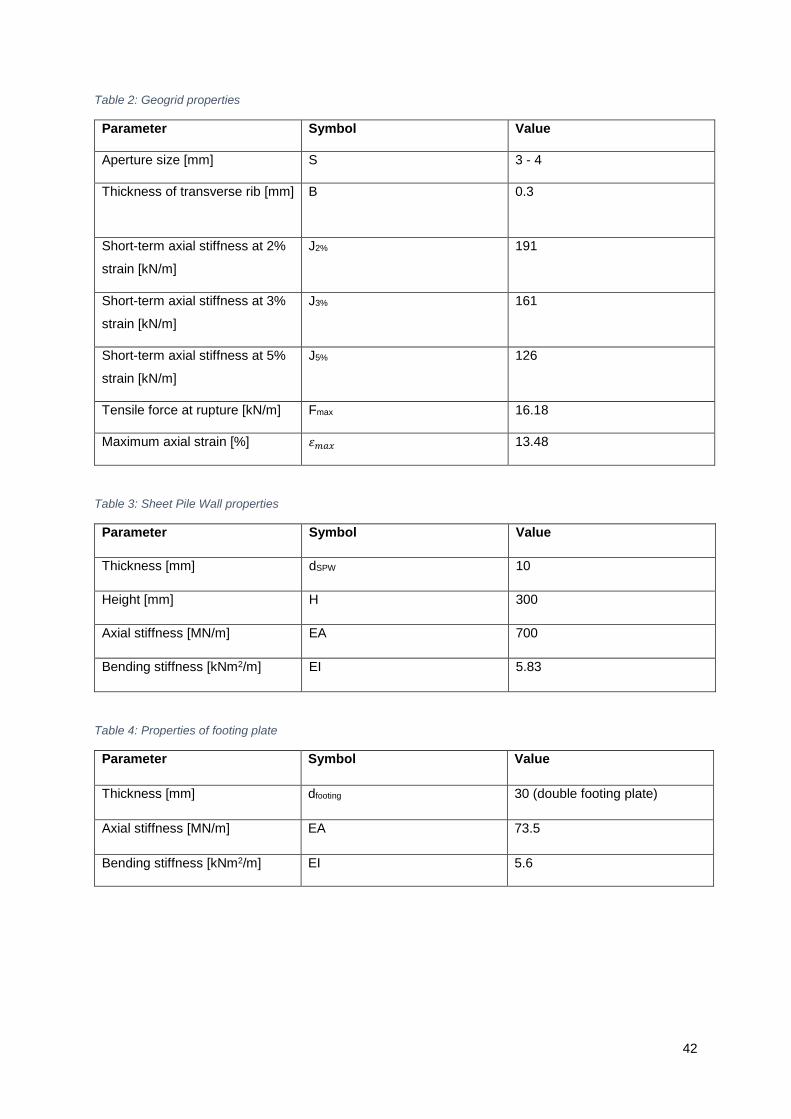
42
Table 2: Geogrid properties
Parameter Symbol Value
Aperture size [mm] S 3 - 4
Thickness of transverse rib [mm] B 0.3
Short-term axial stiffness at 2%
strain [kN/m]
J2% 191
Short-term axial stiffness at 3%
strain [kN/m]
J3% 161
Short-term axial stiffness at 5%
strain [kN/m]
J5% 126
Tensile force at rupture [kN/m] Fmax 16.18
Maximum axial strain [%] 휀𝑚𝑎𝑥 13.48
Table 3: Sheet Pile Wall properties
Parameter Symbol Value
Thickness [mm] dSPW 10
Height [mm] H 300
Axial stiffness [MN/m] EA 700
Bending stiffness [kNm2/m] EI 5.83
Table 4: Properties of footing plate
Parameter Symbol Value
Thickness [mm] dfooting 30 (double footing plate)
Axial stiffness [MN/m] EA 73.5
Bending stiffness [kNm2/m] EI 5.6

43
Table 5: Properties of silicone block
Parameter Symbol Value
Height [mm] Hsilicone block 50
Young’s modulus [MPa] E 159
6.2 Measurement set up
DPIV requires as input data photos in which the development of soil deformation is captured during the
test. A Canon EOS 750D camera with a resolution of 24 megapixels (6000 x 4000) is positioned on a
tripod in front of the test box as depicted in Figure 35a. Two artificial light sources were used to illuminate
the test box. Variation in illumination due to daylight and shadows of moving objects was prevented by
placing a large white plate behind the test box and a large plate in front of the camera (with a hole in it
for the camera). The area captured on the photo is limited to the test box. Every five seconds a photo is
taken from the start to the end of the test. Also, the deformation of the SPW is tracked on the basis of
the photos. A black line was drawn on the white sealing strip at the side of the SPW (see Figure 35b),
which could subsequently be tracked due to the colour difference. The magnitude of the surcharge load
at each photo was derived from the known time and water flow rate (the weight of the inflowing water
was measured in time). Soil deformations that were calculated from the difference between subsequent
photos were used to assess the influence of the geogrid-anchorage on the total stability of the SPW-
retained soil mass. Besides variations in length and number of geogrids, the position of the surface load
has been varied in order to investigate the relation between the position of the load and the mobilised
anchor force.
Figure 35: a) Camera set-up b) SPW with black line on white sealing strip.

44
6.3 Test preparation procedure
Each test was set-up according to the following steps:
1. The sidewalls of the test box were lubricated and a silicone sheet was placed against both
sidewalls.
2. The silicone block and sheet pile wall were placed in the test box.
The geogrids were connected to the SPW by clamping the front part between a small metal
plate and the SPW (see Figure 36). By clamping the forces will be equally distributed
along the width of the geogrid.
3. The sheet pile wall was prevented to deform by placing a clamp between the top of the sheet
pile wall and the front wall.
4. Dry Baskarp B15 sand was gradually poured in the test box and simultaneously densified by
means of tamping.
5. When the sand body was at the height of the geogrid, the surface of the sand body was first
flattened before unfolding and placing the geogrid on top.
6. The geogrid was stretched tight while pouring sand on top of it.
7. When the sand preparation was completed, the top surface was flattened, and the acrylate
footing plate was placed at the desired location on top of the sand.
8. A second footing plate was placed on top, with in between the two footing plates a rod to allow
the lower footing to deform under the soil movement.
9. The bucket was placed on a guidance frame on top of the upper footing plate.
10. The artificial light sources were switched on, the camera positioned, and camera settings were
checked.
11. Just before the test started, the clamp was removed to make free movement of the SPW
possible.
12. The first photo was taken at the start of the test i.e. at zero water volume in the bucket. The
initial load was equal to 4.4558 kg, which is the total weight of the double footing, rod, guidance
frame and empty bucket.
13. The moment the first photo was taken, the pump was switched on and the time was tracked
double by a timer and the time was recorded at each saved photo.
14. The water was pumped out of a tank, which was placed on a balance, into the bucket.
Accordingly, the weight of the water in the tank was noted during the test. Based on the
measured weight and time, the flow rate was checked and the load level was determined during
the test. During the tests, the constant flow rate was equal to a flow rate in the range of 0.02-
0.04 kg/s. A maximum applied load of around 65 kg (65 kPa for the 10 cm by 10 cm footing)
was reached if no failure occurred at an earlier stage.

45
Figure 36: Geogrid-SPW connection

46
7 Boundary effects
In this chapter, we investigate to what degree the stresses and strains in the soil are affected by
boundary effects in the small-scale experiment. Since the test box is very narrow (0.1 m), the influence
of the sidewall friction on the stresses in the soil is expected to be large. The surcharge load will be
transferred partly to the sidewalls, which affects the soil stresses and strains in the soil. Knowledge of
the magnitude of the frictional force is of importance to know to what degree the stresses in the soil
deviate from the stresses under true plane strain conditions. The theory behind the interaction of soil,
surcharge load and sidewalls is shortly discussed in Section 7.1. Section 7.2 gives the results of two
test set-ups, by which the interface friction angle between sand and sidewall is determined. Additionally,
the results are discussed of a third test set-up, which is devised to measure the total vertical force
transferred to the sidewalls. In Section 7.4 and 7.5, we substantiate why the influence of the back-wall
and the silicone sheet on the sliding of the active soil body can be neglected.
7.1 Frictional forces & the arching effect
The surface area of acrylate sidewalls has a certain roughness. Movement of the granular soil along the
sidewall will consequently induce friction. Due to these shear stresses between the walls and soil,
vertical pressures are transferred to the sidewalls. The maximum frictional force which can develop
before the soil starts to slide along the sidewall is determined by the normal force exerted by the soil
onto the sidewalls and the friction angle between the soil and sidewall. The normal force is described
by the vertical pressure in the soil and the horizontal to vertical soil stress ratio, Ksw. The value of Ksw
depends on the internal friction angle, stress history and current stress state.
Friction between sand and walls does not only affect the shear band of the soil adjacent to the walls.
Studies on the pressure development of the soil within a constrained space originate from the late 19th
century. Commonly known and still widely applied is Janssen’s arching theory. He investigated the
pressure of silos filled with grain or corn (Janssen, 1895).
Figure 37: Silo effect according to Janssen’s theory (Khosravi, Kargar and Pipatpongsa, 2018).

47
Figure 37 shows the effect of the induced friction between the bulk solid and walls on the pressure
distribution with depth. The frictionless interface between the fluid at rest and the walls show a linear
pressure distribution, i.e. hydrostatic conditions. Friction between the granular soil and walls is induced
due to settlement of the soil. In our experiment, the test box was gradually filled with sand.
Simultaneously, the sand was densified by means of tamping. Soil self-weight settlement is therefore
expected to be small. Tamping close to the walls may induce friction, however most friction is expected
to develop when the surcharge load is applied.
The shear stresses generated between the sidewall-sand interface cause a re-orientation of the principal
stresses as depicted in Figure 38 (Khosravi et al, 2018). Since the test box is narrow, a full ‘arch’ in the
soil is expected to develop. Consequently, vertical pressures will be reduced over the entire soil area.
Figure 38: Soil arching principle (Khosravi et al, 2018).

48
7.2 Measuring Sidewall Friction
In our experiments, the friction between sand and the acrylate sidewalls was reduced by lubricating the
sidewalls with a low friction substance and placing a highly adhesive, transparent silicone sheet between
the lubricated sidewalls and sand. It was opted to create full adhesion between the silicone sheet and
sand, while creating a frictionless interface between the silicone sheet and the acrylate sidewalls of the
test box. For a couple of tests, the silicone sheet was marked with black dots in the area with large soil
deformation. The relative displacement between the silicone sheet and sand is subsequently examined
by manually tracking the black markers on the silicone sheet from the digital photos taken during the
test. The relative displacement between the black markers and the soil is determined to be smaller than
0.3 mm. Considering the small relative displacement, we assume that the sand and silicone sheet
deform as a unity i.e. a fully rough interface. Consequently, the friction between the sand and sidewall
is equal to the friction between the silicone sheet and sidewall. This also means that the derived sidewall
friction angle (𝛿𝑠𝑖𝑑𝑒𝑤𝑎𝑙𝑙,𝑠𝑎𝑛𝑑) is equal to the interface friction angle between the silicone sheet and
acrylate sidewall (𝛿𝑠𝑖𝑑𝑒𝑤𝑎𝑙𝑙,𝑠𝑖𝑙𝑖𝑐). Therefore, we can refer to the interface friction angle between the sand
and acrylate sidewalls with one symbol 𝛿.
Two different test set-ups were used to measure 𝛿, namely the ‘Spring Suspension test’ and ‘the Pull-
up test’. Besides the water-based lubricant, which has finally been used for the small-scale experiments,
three other substances and a combination of two substances were also tested in the Spring Suspension
test. The friction coefficient for the water-based lubricant was considered sufficiently low, although up to
~45% lower friction coefficients were found for some of the other substances. The overriding factor in
choosing the water-based lubricant above the other substances was the high transparency of this fluid.
High transparency is very important for the DPIV analysis, which requires high resolution images of the
sand behind the sidewall. The two tests and the measured interface friction angle are explained briefly
below. A more detailed description can be found in Appendix A1 and Appendix A.2. A third test, the
‘Stress-transducer test’, was conducted to measure the loss of vertical pressure in the soil at the bottom
of the test box due to sidewall friction as a function of applied surface load. These measurements are
conducted during a small-scale experiment without geogrids, such that the influence of the geogrids is
removed. The combination of tests leads to a reliable estimation of the influence of the sidewall friction
on the soil stresses and strains at a particular surface load in the small-scale experiment.

49
7.2.1 Spring suspension test
Figure 39 depicts the test set-up of the Spring-Suspension test. The test consists of a 5 kg weight, spring
balance and electromotor. The interface between the lubricated acrylate sidewall with a silicone sheet
placed against it, is mimicked in this test by gluing the silicone sheet on the bottom of the weight and
placing the weight on top of the lubricated acrylate plate. The spring balance is on one side connected
to the weight and on the other side to the electromotor.
Figure 39: Spring suspension test
The static friction coefficient between the acrylate wall and silicone sheet is defined as the horizontal
force required to get the weight into motion relative to the normal force. The dynamic friction coefficient
is defined as the horizontal force required to maintain the weight in constant motion relative to the normal
force. We defined the dynamic friction coefficient by the force required to pull the weight forward at a
travelled distance of 5 cm. Figure 40 shows the results of the static friction coefficient for all substances,
which have been tested. The results are represented as a boxplot where the dots are extreme values in
the data. The median of the static friction coefficient and dynamic friction coefficient of the water-based
lubricant is 0.09 and 0.08 respectively. The maximum frictional force which can develop between the
sand and sidewall, or actually the silicone sheet and sidewall, is determined by the highest friction
coefficient. The interface friction angle is derived from the friction coefficient according to equation 7.1:
𝜇𝑠𝑡𝑎𝑡𝑖𝑐 = tan(𝛿) =𝐹𝑓
𝐹𝑁= 0.09(7.1)
in which𝐹𝑁 is the normal force exerted by the weight on the acrylate plate, 𝐹𝑓 is the frictional shear force
acting between the bottom surface area of the weight and the acrylate plate, 𝐹𝑓 is equal to the measured
horizontal force as the inclination between the sliding direction of the weight and the horizontal pulling
force is zero.

50
According to the results of the spring suspension test, the mean value of interface friction angle 𝛿
between the sand and sidewalls in the small-scale experiment is equal to 4.8° with a standard deviation
of 0.014°.
Figure 40: Results of static friction coefficient from spring suspension test. The substances that have been tested are Driehoek hand soap (A), water-based lubricant (B), Petroleum Jelly (C ), a combination of Petroleum Jelly on the acrylate and water-based lubricant on the silicone (D), silicone oil (E), and Dreft dishwashing liquid (F).

51
7.2.2 Pull-up test
Another test-set up, named the ´pull-up test´, was devised to measure the total sidewall force. The test
set-up is depicted in Figure 41.
Figure 41: Photo of test set-up of box without bottom
The concept of the pull-up test is to determine the vertical force transferred to the sidewalls by measuring
the difference between the force required to pull up the test box (without bottom) only and to pull-up the
test box (without bottom) prepared with sand in combination with or without an additional known
surcharge. An overhead crane enables measuring the total weight of the test box, which is connected
to the test box and lifts it up vertically. By incorporating a load cell within the connection of the overhead
crane and the test box, the required force to lift the test box is measured. A duplicate test box, but with
an open bottom, is filled with sand. The preparation procedure of densifying the sand is identical to the
small-scale experiment with relative densities in the same range of 70% ± 12%. Both sidewalls and the
front-and back wall of the test box were lubricated and covered with a thin silicone sheet in accordance
with the preparation procedure of the sidewalls in the small-scale experiment.
The relations proposed by Bathurst and Benjamin (1987) between the total sidewall frictional force,
geometry of the test box, surcharge load, volumetric weight of the sand, horizontal earth pressure
coefficient and interface friction angle are implemented to derive 𝛿 from the measured total sidewall
frictional force 𝑋𝑚𝑒𝑎𝑠𝑢𝑟𝑒𝑑 . The analytical solution is included in Appendix A.2. Here, we will only discuss
the results.

52
Figure 42 gives the results of the pull-up test for the test without silicone sheets on the sidewalls and
the test with silicone sheets on the sidewalls. From the test with silicone sheets on the sidewalls,
denoted by the red line, we conclude that the total vertical force transferred to the soil is 52%. Hence,
48% of the total load is transferred to the sidewalls.
Figure 42: Test results of pull-up test.
Figure 43 gives the difference between the measured sidewall frictional force and analytical solution for
different interface friction angles (𝛿) and an internal friction angle (𝜑) equal to:
• 34°, which is the interal friction angle at critical volume (𝜑𝑐𝑣).
• 45°, which is the secant internal friction angle derived from triaxial tests at a confining pressure
of 40 kPa. The confining pressure ranged between 5 kPa – 65 kPa in the small-scale
experiment.
• 50°, which is the peak internal friction angle (𝜑𝑝).
The lateral earth pressure coefficient against the sidewalls, 𝐾𝑠𝑤 , is estimated within the range of 0.3 –
0.5 for an internal friction angle of 45°. The analytical solution proposed by Bathurst and Benjamin (1987)
agrees with the measured value for an interface friction angle, 𝛿, of 12.7° (for 𝜑 = 45°).

53
Figure 43: Difference between the measured sidewall frictional force and analytical solution for different interface friction angles (𝛿) and an internal friction angle (𝜑).
This test was for comparison reasons also performed without silicone sheets on the sidewalls such that
the sand is in direct contact with the acrylate sidewall. For the lower bound and upper bound value of
𝐾0 and an internal friction angle of 45°, values of 18.7° and 16.2° were determined for the interface
friction angle. Previous studies determined an interface friction coefficient of 15° between sand and
glass sidewalls (Jacobs et al, 2016). Assuming that the friction coefficient between sand and acrylate is
similar to sand and glass, it can be stated that the results are reliable within an error margin of several
degrees.
The pull up tests indicated that the added lubricant is effective in reducing the friction from 16°-18° to
12.7°. The spring suspension tests resulted in lower values.
The interface friction angle between sand and sidewall determined with the pull-up test is 2.5 times
larger than the one determined with the spring-suspension test. Both tests have their inaccuracies and
deviating conditions from the small-scale experiment. The precision of the Spring Suspension test turned
out to be high as the standard deviation is only 0.3% from the mean friction angle. The precision of the
Pull-up test is difficult to determine as only one test has been performed. The accuracy depends on the
assumptions made for determining the interface friction angle and whether those are plausible. The
advantage of this test is that the sand-silicone sheet-acrylate sidewall interface is identical to the small-
scale experiment.

54
Potential differences in the test conditions between the pull up and spring suspension test with the small-
scale experiments could lead to a different interface friction angle in practice. These are the duration of
test, thickness of the layer of lubricant on acrylate plate, temperature and normal pressure. The duration
of the small-scale experiments varied between 10 minutes and 35 minutes, depending on the length
and number of layers of the geogrid-anchorage. Over time, the film of lubricant may dry out as a
consequence of the artificial light sources which exert heat. Also, the film of lubricant may become
thinner over time as the lubricant is squeezed out due to the pressure of the soil or absorbed by the
silicone sheet. Furthermore, the temperature and normal pressure could be of influence because the
viscosity of the lubricant may be influenced by temperature differences and pressure differences
between the spring-suspension test and small-scale experiment. Literature has been used to get an
indication to what degree the interface friction angle could deviate between these two tests - in which
the friction angle is derived - and the small-scale experiment due to temperature and pressure
differences. Based on literature, it is concluded that pressure and temperature differences between the
tests and the small-scale experiment play no role. This conclusion is elaborated in Appendix A.3.
7.2.3 Stress-transducer test
In order to obtain more certainty with regard to the sidewall frictional forces, a third test set-up, called
the Stress-transducer test, is conducted. The total sidewall frictional force measured with the Pull-up
test will not be equal to the total sidewall frictional force in the small-scale experiment. Since both
sidewalls and the front-and back wall were lubricated and covered with silicone sheets, only the friction
coefficient of the interface lubricated acrylate wall - silicone sheet – sand is present. However, different
friction coefficients are present in the small-scale experiment as the front wall is ‘replaced’ by the SPW
and the back wall is in direct contact with the sand. Moreover, the soil in the Pull up test is subjected to
a uniform surcharge, while the soil in the small-scale experiment is subjected to a strip footing load.
Since the interfaces and loading type of this test is identical to the small-scale experiment, a better
insight will be obtained into the magnitude of the total sidewall frictional force.
Since pressure cells did not proof to be reliable at the low range of soil pressures in our test set-up, an
alternative method based on the measurement of water level differences in stand-pipes is adopted.
Details about the measurement can be found in Appendix A.4.
In order to measure the weight loss due to friction with the sidewalls, the footing of the surcharge load
was placed in the middle of the test box to avoid influence of the sheet pile wall. No geogrids were
connected to the SPW, which could transfer vertical stresses to the SPW.
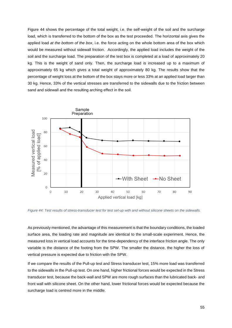
55
Figure 44 shows the percentage of the total weight, i.e. the self-weight of the soil and the surcharge
load, which is transferred to the bottom of the box as the test proceeded. The horizontal axis gives the
applied load at the bottom of the box, i.e. the force acting on the whole bottom area of the box which
would be measured without sidewall friction. Accordingly, the applied load includes the weight of the
soil and the surcharge load. The preparation of the test box is completed at a load of approximately 20
kg. This is the weight of sand only. Then, the surcharge load is increased up to a maximum of
approximately 65 kg which gives a total weight of approximately 80 kg. The results show that the
percentage of weight loss at the bottom of the box stays more or less 33% at an applied load larger than
30 kg. Hence, 33% of the vertical stresses are transferred to the sidewalls due to the friction between
sand and sidewall and the resulting arching effect in the soil.
Figure 44: Test results of stress-transducer test for test set-up with and without silicone sheets on the sidewalls.
As previously mentioned, the advantage of this measurement is that the boundary conditions, the loaded
surface area, the loading rate and magnitude are identical to the small-scale experiment. Hence, the
measured loss in vertical load accounts for the time-dependency of the interface friction angle. The only
variable is the distance of the footing from the SPW. The smaller the distance, the higher the loss of
vertical pressure is expected due to friction with the SPW.
If we compare the results of the Pull-up test and Stress transducer test, 15% more load was transferred
to the sidewalls in the Pull-up test. On one hand, higher frictional forces would be expected in the Stress
transducer test, because the back-wall and SPW are more rough surfaces than the lubricated back- and
front wall with silicone sheet. On the other hand, lower frictional forces would be expected because the
surcharge load is centred more in the middle.

56
Finally, we consider the results of the Stress tranducer test as most representative for the sidewall
friction developing in the small-scale experiment. Therefore, we assume that 33% of the total weight is
transferred to the sidewalls in the small-scale experiment. The same analytical relations proposed by
Bathurst and Benjamin (1987) as were used for the derivation of the sidewall friction angle 𝛿 from the
Pull up test are modified and used to find out how either the small-scale experiment or plane strain
numerical model can be best adjusted in order to correct the results for sidewall friction (see Chapter
10.2). By means of these relations, it is determined which sidewall friction angle, the one derived from
the Spring suspension test or the Pull-up test, best fit the measured frictional force derived from the
Stress-transducer test. The value of the sidewall friction angle will lie between 4.8° and 12.7°.
7.3 Effect back wall on earth pressures against SPW
Since the spacing between the SPW and back wall is four times larger than the spacing between the
sidewalls, the arching effect induced by the interaction of the soil with the sidewalls is dominant. The
arching between the back and front wall only contributed minimally to the total frictional forces in the
pull-up test. Yang and Liu (2007) showed that the arching effect is negligible for a ratio of the spacing
between the walls to the height of the wall larger than 0.7. In the small-scale experiment, the distance
between the back wall and SPW is 0.415 m and the height of the SPW is 0.3 m. This gives a ratio of
1.38, which indicates no influence of the back wall on the earth pressures in the soil.
7.4 Influence silicone sheet on sliding of active zone
Sliding of the active soil body behind the SPW causes tensile stresses in the silicone sheet. The silicone
sheet on the sidewall moves together with the active soil body, while it is kept in place by the soil
pressures behind the active zone.
Whether soil displacements are significantly reduced by the tensile resistance of the silicone sheet, is
deduced from the difference in tensile stiffness of the silicone sheet and the shear modulus of the
Baskarp B15 sand.
The tensile stiffness of the silicone sheet is determined by means of three simple extension tests.
Appendix A.5 describes the test set-up, results and calculation of the tensile stiffness.
The average tensile stiffness 𝐸𝑇 of the silicone sheet is determined to be 0.3 MPa at a strain of 3%. For
comparison, 3% strain corresponds to approximately 1 cm extension of the silicone sheet along the
critical slip surface. The shear modulus of Baskarp B15 sand is derived from Drained Compression
Triaxial tests for a relative density of around 80%. Triaxial tests were performed for confining pressures
ranging between 5 kPa and 320 kPa (Ibsen, 2009). The relation between the confining pressure and
Young’s modulus is defined by the parameter m in equation 7.2.

57
𝑚 =ln(
𝐸50𝑟𝑒𝑓
𝐸50)
ln(𝜎3𝑟𝑒𝑓
𝜎3)
(7.2)
Here, 𝐸50𝑟𝑒𝑓
is the Young’s modulus at a confining pressure 𝜎3𝑟𝑒𝑓
of 100 kPa. The power m has been
determined to be equal to 0.54. Slipping of the soil body occurred at a surcharge load of 2-3.5 kN//m.
According to the 2V:1H approximate method, the average confining pressure is estimated to be
approximately 3 - 4 kPa for a strip footing load, which corresponds to a Young’s modulus of 7-9 MPa.
The Shear modulus can be derived according to Hooke’s law:
𝐺 =𝐸
2(1 + 𝜗)(7.3)
Here, E is the Young’s modulus equal to 8 MPa, 𝜗 is Poisson’s ratio equal to 0.25 and G is the Shear
modulus, which is calculated to be 3.2 MPa.
Concludingly, the shear modulus of the soil is around 10 times larger than the tensile stiffness of the
silicone sheet. Assuming again the elastic stress-strain relationship of Hooke’s law such that the shear
stress is described by the shear modulus and the shear strain according to equation 7.4.
𝜏𝑥𝑦 = 𝐺𝛾𝑥𝑦(7.4)
Then, the resisting tensile stress of the silicone sheet against sliding of the active soil body is around 10
times lower with respect to the magnitude of the shear stresses required to develop the critical slip
surface in the soil. No correction of the soil displacements for the resisting forces of the silicone sheet
are deemed necessary.
58
8 Digital Particle Image Velocimetry (DPIV)
In our small-scale tests, Digital Particle Image Velocimetry (DPIV) techniques were used to determine
the deformations of the sand body and the sheet pile wall. DPIV techniques have been widely employed
for the computation of full-field soil displacements in experimental set-ups. For our tests, a digital
photograph (image-) sequence with an interval of five seconds is assembled during the tests, which is
used as input data for the algorithms and analysis techniques that underpin DPIV.
Section 8.1 describes the factors which are decisive for the achieved precision and accuracy of the soil
displacements. In Section 8.2, three different DPIV software; OpenPIV (Liberzon, Gurka and Taylor,
2020), GeoPIV-RG (Stanier et al, 2015b) and PIVlab (Thielicke, 2019), are utilized in order to investigate
the influence of computational details of the DPIV software on the accuracy of the soil displacements.
Based on these results, we decide which of the three DPIV software will be used for the analyses of the
test results. Furthermore, the results obtained for different sets of input values of the user-defined DPIV
parameters have been analysed and compared. This analysis is worked out in Section 8.2. Lastly, in
Section 8.3, we explain the procedure to calculate the axial strains in the geogrid by means of the soil
displacement results from DPIV in Section 8.3.
8.1 Factors influencing the accuracy of DPIV
To calculate the soil displacements, DPIV uses digital image correlation (DIC) algorithms that finds
correspondences between the pixels of a grey-scale image pair A-B. Image A is subdivided into smaller
interrogation areas and the particle pattern of each interrogation area is traced back in image B by
means of cross-correlation. The peak value of the correlation matrix is assumed to be the new location
of the interrogation window in image B (Thielicke, 2014). The displacement is the distance between the
location of the interrogation window in image A and the new location in mage B. If the new locations of
all interrogation areas of the reference image can be detected in subsequent images, the displacement
of every interrogation area can be computed.
Previous studies, such as (Stanier, Blaber, Take and White, 2016), (Wood, 2012), (Dijkstra et al., 2008),
(Thielicke, 2014), (Teng, Stanier and Gourvenec, 2016), (Chen, Omidvar and Iskander, 2016) suggest
that several factors may influence the accuracy of the soil displacements derived with DPIV, like
• the resolution of the image,
• the photogrammetric correction,
• the sand particle size to pixel ratio,
• the image texture quality,
• computational details such as the cross-correlation algorithm,
• order of shape functions,
• subpixel peak estimator and
• the choice of the values for the user-defined input parameters may unwittingly lead to
inaccuracies due to spurious numerical artefacts (Stanier et al, 2016).

59
Hence, thorough consideration must be taken for the choice of the input parameters. The following
paragraphs discuss each of these factors.
8.1.1 Resolution of the image
A Canon EOS 750D camera with a resolution of 24 megapixels (6000 x 4000) was positioned on a tripod
in front of the test box, approximately 1 m spacing in between. Although the exposure settings slightly
varied between the tests, the general settings used were a ISO-speed of 100, relative aperture of f/6.3
and shutter speed of 1/125 sec. The area captured on the photo was limited to the test box. Full use of
the 6000 x 4000 pixels was not possible due to:
• differences in aspect ratio between the box and the camera image
• restraints with respect to positioning the camera.
Therefore, the effective area of the region of interest was 4000 to 2800 pixels. The area slightly varied
per test due to camera positioning (about 200 pixels horizontal and/or vertical). The exposure settings
of relative aperture (the focal length with respect to the absolute aperture size), shutter speed and ISO
speed were chosen such that:
• noise is minimalized
• the contrast in pixel intensity is optimized.
The latter indicates that the most frequent intensities of the image histogram are spread out as much as
possible to the full range of the data, i.e., from 0 to 255 in 8-bit images. Intensity histograms with a
uniform distribution were obtained. Figure 45 shows the normalized histogram of the pixel intensity
distribution of one of the tests with values between 38 and 243. A range of values between 20 and 255
is considered as a high-quality image (Stanier et al, 2016).
It is concluded that our digital photographs are of sufficient quality in order to derive the soil
displacements using DPIV.
Figure 45: Histogram of pixel intensity values for which the soil domain only is included (right).

60
8.1.2 Photogrammetric correction
A photogrammetric correction aims to solve camera lens distortions and relative movements between
the camera and the test model, which would lead to errors in the conversion of image space units (pixels)
to object space units (mm) (Teng et al, 2016). For the calibration to object space units, the mathematical
models incorporated in the DPIV software in order to correct for photogrammetric distortion were not
utilized as we expect the photogrammetric distortion to be minimal. There is no rotational or translational
movement between the camera and test model during the test. Furthermore, ArUco markers were
placed on the test box at the corners of the soil domain as depicted in Figure 46. These markers serve
as a fiducial marker system, which can be used for camera pose estimation (Garrido-Jurado et al, 2014).
Subsequently, a mathematical correction could be applied to offset the in-plain misalignment of the test
box relative to the camera. Prescribed functions were implemented to detect the four ArUco markers
and calculate the transformation matrix to transform the image coordinates of the center of the ArUco
markers to the corrected image coordinates such that the ArUco markers form a surface parallel to the
camera surface (OpenCV team, n.d.).
Figure 46: Example image of image sequence during one of the experiments. Figure 10a shows the original photo. Figure 10b shows the image after a perspective transformation. Note that the three dots on the right sight of the soil domain were for some tests additionally applied on the silicone sheet in order to determine the relative displacement between the silicone sheet and sand (see the chapter ‘Boundary effects’ for more information).
Lens distortion is expected to be of minimal influence on the computed soil displacements because of
three reasons. First, we expect that the camera-lens-induced distortions do not change during the
experiment, because (a) the lens is not subjected to stress changes in a 1g experiment and (b) the
incidence of light is controlled by artificial light sources and by simultaneously blocking daylight.
Accordingly, erroneous displacement computations can only occur due to:
1. a difference in calibration factor (from pixels to metric units) between the area of the image
frame where the soil displacements take place and the area of the image frame where the
calibration factor is determined actually, and
2. ‘local’ lens distortion.

61
With ‘local’ lens distortion, lens distortion on the scale of the soil displacements is meant. Due to local
lens distortion, DPIV will compute ‘lens-distorted’ displacements which may deviate from the true
displacements. Second, the lens distortion is investigated by comparing the original image with the
image, which is corrected for lens distortion. In order to investigate to what degree the image is distorted,
a picture was taken from a chessboard of which the distance between the corners of all squares are
known. By means of prescribed functions, the tangential and radial lens distortion has been determined
(OpenCV Team, 2019). A mean total lens distortion of 0.15% has been computed.
The horizontal – and vertical calibration factor is determined by the known distance in metric units
between the black stripes on the sidewall and the measuring tape glued on the inside of the sidewall
(see Figure 46). The error in the calibration factor will be close to the mean lens distortion of 0.15%.
In the area close to the SPW, where most soil deformation takes place, the ‘local’ lens distortion is
smaller than 1 pixel (i.e. difference between coordinates of corrected and non-corrected image).
Therefore, it can be stated that the error of the displacements will be close to 1 pixel (approximately 0.1
mm). Third, the image is corrected for tangential lens distortion because the pixel values have been
interpolated (bilinear interpolation) between the corrected image coordinates in order to perform the
perspective transformation of the image (OpenCV team, n.d.). Therefore, the total lens distortion will be
smaller than the lens distortion determined with the images of the chessboard.
Concludingly, the benefit of a photogrammetric correction does not outweigh the negative consequence
of obscuring to a larger extent the zone of interest because of the need of more calibration points. Figure
46 shows an example image of one of our experiments in the small-scale test box. The horizontal – and
vertical calibration factor is determined by the known distance in metric units between the black stripes
on the sidewall and the measuring tape glued on the inside of the sidewall.
8.1.3 Cross-correlation algorithm
Thielicke (2014) gives two approaches to solve the discrete cross-correlation function for two discretely
sampled images. The first approach is to solve the discrete cross-correlation function in the spatial
domain, which is commonly known as Direct Cross-Correlation (DCC). The second approach solves the
discrete cross-correlation function in the frequency domain by fast Fourier transformations. This
approach is known as Discrete Fourier Transform (DFT) (Thielicke, 2014) (Pust, 2006). The DFT was
introduced as a cross-correlation function solver to reduce the computation time (Pust, 2006). However,
this advantage out weights the reduced accuracy as demonstrated by the analysis of (Thielicke, 2014),
who compared the results obtained with DCC and DFT. The reduced accuracy is a consequence of the
requirement that the search area in image B must be of identical size as the interrogation window in
image A for the DFT to work properly. As a result, soil displacement will be lost as every translation or
rotation can never be fully captured (Thielicke, 2014). Additionally, erroneous correlation matrices can
be computed when soil displacements are large relative to the size of the interrogation window. The
underlying Fast Fourier transform (FFT) converts the intensity values enclosed by each spatial
interrogation window to a representation in the frequency domain. The intensity values are described
by a periodic function as a result. The intensity peak value, corresponding to the new location of the
62
interrogation window, will be folded back if the displacements are larger than half the size of the
interrogation window (Thielicke, 2014). Because DCC is well defined for finite regions and can cope with
different interrogation window and search area sizes in contrast to DFT, these risks do not apply for
DCC. The accuracy and precision of the DFT approach was improved by introducing multiple passes
(Thielicke, 2014). The displacement is computed by running several passes of the DFT, whereby the
size of the interrogation window is relatively large for the first pass and smallest for the last pass
(Thielicke, 2014). The results of the first pass are used to optimize the location of the search area of the
second pass. The drawback of the improved accuracy of this method is that the computational time will
be increased
8.1.4 Shape functions
Shape functions are used to deform the interrogation window such that the correlation of the image pair
is optimized. The order of deformation of each interrogation window which can be computed depends
on the order of the shape function. When zero-order shape functions are used to relate image
coordinates in image A to coordinates in image B, only pure translation of the interrogation window can
be computed. First-order shape functions allow the interrogation window to deform by translation,
rotation, shear and normal strains (Schreier and Sutton, n.d.). More complicated deformations can again
be computed with higher-order deformations. If the soil deformations are of higher order, higher
precision and accuracy will be achieved with higher order shape functions. Also, ‘random walk errors’
will be reduced (Stanier et al, 2016). These errors have to do with the computation scheme of all images
captured during the test. We will elaborate on the random walk errors when we discuss the computation
scheme
8.1.5 Subpixel peak estimator
When the cross-correlation matrix of an image pair is calculated by means of one of the correlation
algorithms, the peak value can be found at integer pixel precision. Because displacements are
continuous functions, a subpixel estimation of the displacements is required in order to prevent large
inaccuracies. The DPIV software makes use of interpolants in order to estimate the peak value at
subpixel precision. A function is chosen which is assumed to best describe the distribution of the cross-
correlation matrix. This function is fitted to the correlation values at integer pixel precision. Accordingly,
the peak estimated by this interpolated function gives the estimated displacement at subpixel precision.

63
Figure 47 shows the principle. Here, a Gaussian distribution is assumed as interpolant (Thielicke, 2014).
The DPIV software differ greatly in the way they estimate the subpixel peak value of the correlation
matrix. But all software uses a form of interpolation. The need to interpolate between the values at
integer pixel precision lead to accuracy errors. These errors will be very small for advanced DPIV
software under the assumption that the image quality is high.
8.1.6 Computation scheme
The displacement is computed between two images. There are different ways to calculate the total
displacement from the first to the last image of the entire images sequence. The first image can be taken
as reference for every image, such that we get the scheme ‘1-2, 1-3, 1-4,..1-N’. Here ‘1’ represents the
first image at the start of the test and N is the last image at the end of the test. This scheme will lead to
accuracy errors when the soil deformations are large (Stanier et al, 2016). DPIV software with first or
higher order shape functions will not suffer from this accuracy loss as the interrogation window can
adapt to the deformed shape. Another option is to update the reference image after every computation
such that the scheme becomes ‘1-2, 2-3, 3-4,..(N-1)-N’. This computation scheme is sensitive for
random walk errors (Stanier et al., 2016). If the updated location of the interrogation window contains
an error, and this location is taken as reference for the computation of the successive image pair, the
errors will add up. In particular, this error will be significant for strains in low deformation zones and small
spacing between the interrogation windows (Stanier et al, 2016). Since strains are the derivatives of the
displacement fields, the errors will amplify. They will amplify even more if the computed displacement
vectors per area increases.
Figure 47: Principle of the subpixel peak estimator technique. The Gaussian 2·3-point fit is employed (Thielicke, 2014).

64
8.1.7 Particle diameter to pixel ratio
The spatial resolution is discrete, because the image data is stored as a pixel array. Every pixel has an
RGB value, which is in de DPIV software converted to one intensity value. On one hand, every grain
must be presented by sufficient pixels such that the displacement of each grain can be computed.
Previous studies recommended a particle diameter to pixel ratio (𝐷50
𝑝𝑖𝑥𝑒𝑙) > 4 to avoid accuracy errors of
the type ‘peak-locking’ (Stanier et al, 2016). The peak-locking effect has to do with the peak finding
calculation procedure. These accuracy errors can become significant if the particle diameter to pixel
ratio is unfavourable.
One can imagine that the correlation values close to the peak value are relatively low if the grains are
not overlapping multiple pixels, which is the case for low values of 𝐷50
𝑝𝑖𝑥𝑒𝑙 . As a consequence, there is
bias in the computed displacements towards the integer pixel value closest to the correlation peak
(Stanier et al, 2016). This bias is generally defined as the ‘peak-locking’ effect. Basically, if the true
displacement is a non-integer pixel value, the interpolation process will fail to correctly calculate the new
location of the interrogation window.
On the other hand, Stanier et al. (2016) and Thielicke (2014) demonstrated that also large accuracy
errors will occur for large 𝐷50
𝑝𝑖𝑥𝑒𝑙 in case the grains lack contrast (Stanier et al, 2016) (Thielicke, 2014). If
a grain is described by multiple pixels and all pixels give similar intensity values as they are of uniform
colour, spurious peaks will develop leading to correlation noise (Stanier et al, 2016).
Analysis of the optimal particle diameter to pixel size ratio in PIVlab showed a local minimum of the error
at a particle diameter equal to 1.8-2 pixels for DCC correlation technique and 3.5-4 pixels for more
advanced window deformation algorithms (DFT correlation technique with multiple passes) (Thielicke,
2014) . A similar analysis in GeoPIV-RG demonstrated that peak-locking is only present for particle
diameters smaller than 2 pixels (Stanier et al, 2016). The latter analysis studied image particle
diameters up to 8 pixels.
The particle size diameter in pixels is not the only cause for potential peak-locking effect. The quality of
the image texture can be a second cause of this effect.

65
8.1.8 Image texture quality – contrast resolution
In particular, the computational precision of the cross-correlation function used to derive the
displacement of each interrogation window between an image pair is greatly influenced by the image
texture (Stanier et al, 2016). Sufficient contrasting pixel values must be present within each interrogation
window such that sufficient information is provided to derive precise correlation. Hence, not only the
resolution in terms of pixels per area is relevant, but also the contrast resolution in terms of intensity
differences between the sand particles. In our situation, the density of the soil is very high and the grains
are relatively small (D50 = 0.137 mm). Since the density is high, very little contrast in terms of light
reflection will be obtained between voids-grains. The contrast resolution relies mainly on the difference
in colour (grey-scale) between the grains. Most contrast was observed between sand grains and the low
share of organic matter in the sand. Figure 48 shows a close up of the soil domain
A measure of the contrast resolution is the standard deviation of the interrogation window intensities 𝜎𝐼𝑠
(Stanier et al, 2016). The standard deviation is computed for an interrogation window size of 100·100,
50·50 and 10·10 pixels in the area below the footing where most deformation is expected.
This resulted in standard deviations of
𝜎𝐼𝑠 ≈ 6.1, 𝜎𝐼𝑠 ≈ 5.2, and 𝜎𝐼𝑠 ≈ 5.8 respectively. According to (Stanier et al, 2016), these are low standard
deviations which results in low precision of the soil displacements as the cross-correlation coefficients
are low.
Figure 49: Different size of interrogation window (from left to right a size of 100·100 pixels, 50·50 pixels and 10·10 pixels) and corresponding standard deviation.
Figure 48: : Close-up of soil domain.

66
8.1.9 User-defined parameters
The parameters which need to be defined by the user is slightly different between the DPIV software.
Here, we will discuss the considerations that must be made when choosing the size of the interrogation
window and spacing between the interrogation windows.
As described above with regard to the contrast resolution, precision of the measurement deteriorates if
the contrast within an interrogation area is too low. The lower bound of the interrogation window size is
defined by the area of the required minimum number of contrasting particles. Stanier et al. (2016)
recommends a minimum of 10 contrasting particles in each direction. This means at least 100 particles
per interrogation window size. For our digital images, 𝐷50
𝑝𝑖𝑥𝑒𝑙 =
0.137𝑚𝑚
0.108𝑚𝑚= 1.3. Accordingly, 1 grain is
presented by 1.3 pixels. Therefore, the lower bound of the interrogation area is 13·13 pixels, which
corresponds with 1.4 mm·1.4 mm. However, we should take note of the fact that not all individual grains
are visible in the image as can be observed in Figure 48. The assumption that each individual grain
provides sufficient contrast is likely not valid. Analyses between different size interrogation windows
must confirm whether larger interrogation areas are required in order to obtain high value correlation
matrices. Figure 49 shows that the contrast did not increase when the size increased from 10·10 pixels
to 100·100 pixels. Therefore, it is expected that the accuracy will not be improved when taking a larger
interrogation window. Meanwhile, a larger interrogation window will have a negative impact on the
accurate computation of the displacements of the shear band along the geogrid. Since this shear band
is expected to be thin, only an interrogation area of similar or smaller thickness can track the
displacement of this shear band properly.
Teng et al. (2016) mentions that the upper bound of the interrogation area is generally defined by the
scale of the local soil deformations (Teng et al, 2016). The soil within each interrogation window is
treated by DPIV as a small portion of soil that deforms continuously. Accuracy errors increase if the local
deformations within the interrogation window becomes significant. These local soil deformations have
been estimated to be of the order of approximately 10D50 (Wood, 2012). Because we use a relatively
small sand particle with a D50 of 0.137 mm, the size of the upper bound of the interrogation window is
similar to the lower bound of the size of the interrogation window. Teng et al. (2016) adds that resolution
images in terms of, 𝐷50
𝑝𝑖𝑥𝑒𝑙 even higher than 4 are likely to be required in order to measure the local
deformations in granular soils (Teng et al, 2016).
Another parameter which must be defined is the spacing between the interrogation windows. Since the
strains are the derivatives of the displacements fields, large overlapping ratio (spacing relative to the
size of the interrogation window) will amplify the accuracy errors of the computed displacement in the
strain results (Stanier et al, 2016). When the overlapping ratio is taken too small, there is a risk that
details will be lost (Stanier et al, 2016). Hence, the accuracy error of the computed displacements must
be evaluated in order to determine for which spacing the error becomes too large.
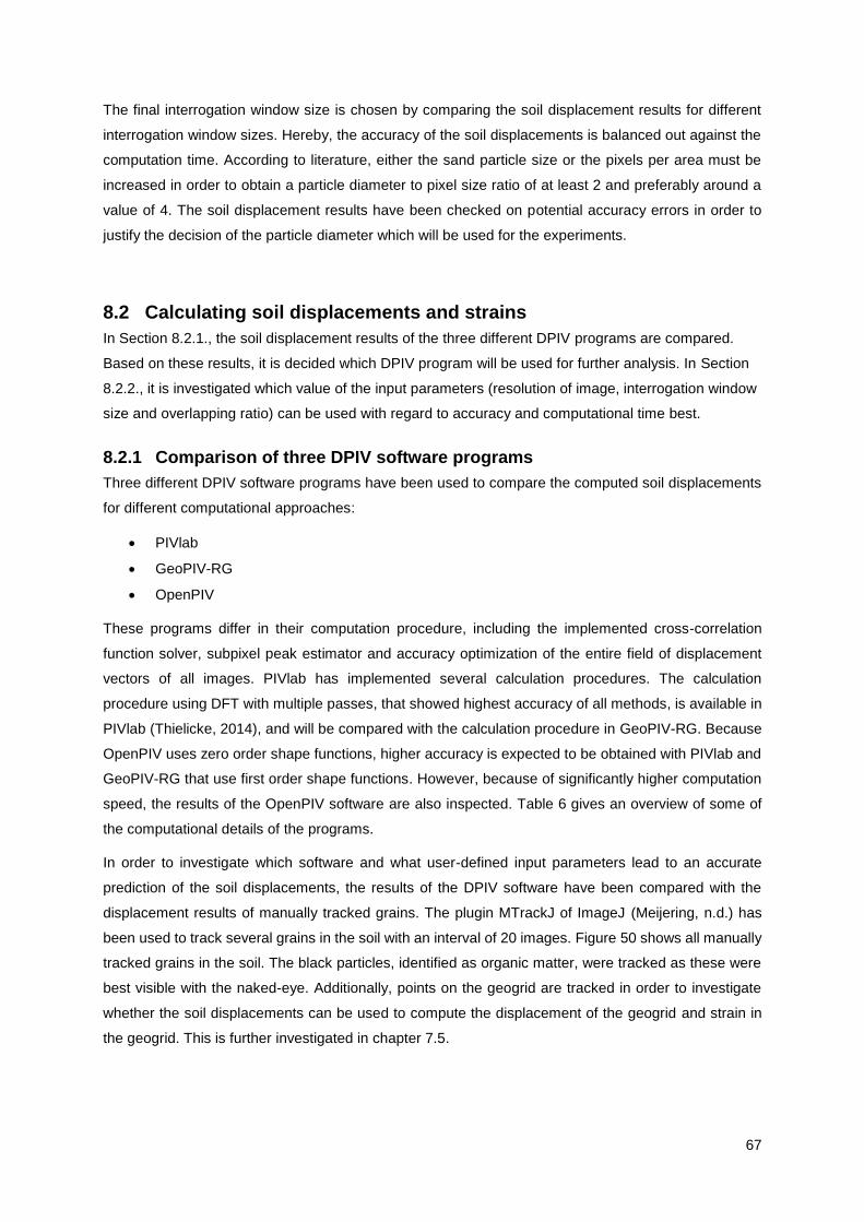
67
The final interrogation window size is chosen by comparing the soil displacement results for different
interrogation window sizes. Hereby, the accuracy of the soil displacements is balanced out against the
computation time. According to literature, either the sand particle size or the pixels per area must be
increased in order to obtain a particle diameter to pixel size ratio of at least 2 and preferably around a
value of 4. The soil displacement results have been checked on potential accuracy errors in order to
justify the decision of the particle diameter which will be used for the experiments.
8.2 Calculating soil displacements and strains
In Section 8.2.1., the soil displacement results of the three different DPIV programs are compared.
Based on these results, it is decided which DPIV program will be used for further analysis. In Section
8.2.2., it is investigated which value of the input parameters (resolution of image, interrogation window
size and overlapping ratio) can be used with regard to accuracy and computational time best.
8.2.1 Comparison of three DPIV software programs
Three different DPIV software programs have been used to compare the computed soil displacements
for different computational approaches:
• PIVlab
• GeoPIV-RG
• OpenPIV
These programs differ in their computation procedure, including the implemented cross-correlation
function solver, subpixel peak estimator and accuracy optimization of the entire field of displacement
vectors of all images. PIVlab has implemented several calculation procedures. The calculation
procedure using DFT with multiple passes, that showed highest accuracy of all methods, is available in
PIVlab (Thielicke, 2014), and will be compared with the calculation procedure in GeoPIV-RG. Because
OpenPIV uses zero order shape functions, higher accuracy is expected to be obtained with PIVlab and
GeoPIV-RG that use first order shape functions. However, because of significantly higher computation
speed, the results of the OpenPIV software are also inspected. Table 6 gives an overview of some of
the computational details of the programs.
In order to investigate which software and what user-defined input parameters lead to an accurate
prediction of the soil displacements, the results of the DPIV software have been compared with the
displacement results of manually tracked grains. The plugin MTrackJ of ImageJ (Meijering, n.d.) has
been used to track several grains in the soil with an interval of 20 images. Figure 50 shows all manually
tracked grains in the soil. The black particles, identified as organic matter, were tracked as these were
best visible with the naked-eye. Additionally, points on the geogrid are tracked in order to investigate
whether the soil displacements can be used to compute the displacement of the geogrid and strain in
the geogrid. This is further investigated in chapter 7.5.
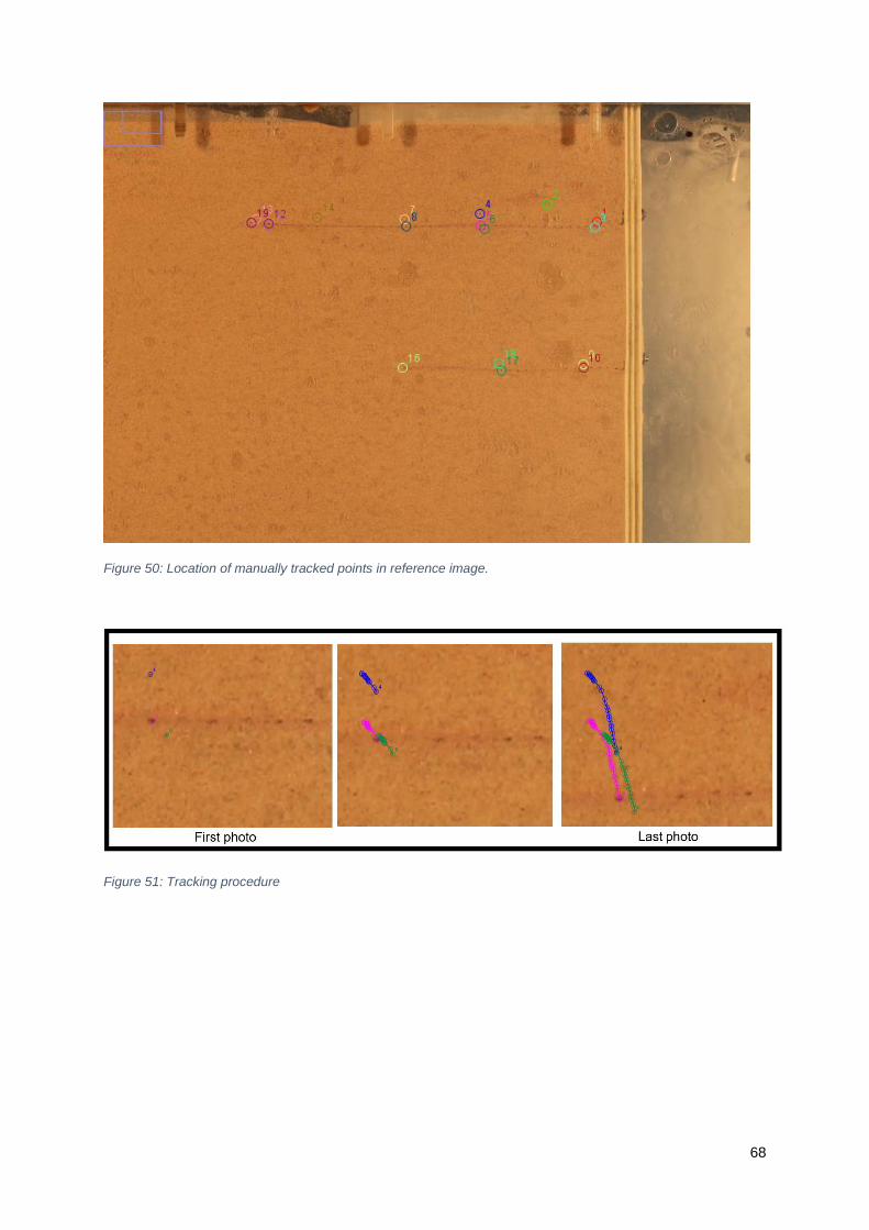
68
Figure 50: Location of manually tracked points in reference image.
Figure 51: Tracking procedure

69
The correlation method, order of shape function and computation scheme of the three DPIV methods,
which have been analysed, are summarized in Table 6. For all methods, the interrogation window and
spacing were set to 40 pixels (≈10.8 mm) and 20 pixels (≈5.4 mm) respectively for an image resolution
of 0.27 mm/pix10. The resolution was reduced by replacing the pixels by 2.5 times larger pixels, which
values were determined by means of bilinear interpolation. Because a bilinear interpolation was applied,
it can be argued that the information of the higher resolution images is inherently included, while taking
into account bias from the interpolation method. Because of a reduction in computational time of
1 -2 days for a resolution of 0.108 mm/pix to a couple of hours for 0.27 mm/pix, the difference between
the three DPIV methods has been examined with the lower resolution.
Table 6: Computational details of the three analysed DPIV methods.
Software DIC method Order of shape function
Computation scheme of image pairs
Size
interrogation window
[pix]
Spacing
between
interrogation
window
[pix]
OpenPIV11 DFT Zero 1-2, 2-3, 3-4,..(N-1)-N 40 20
GeoPIV-RG Normalized DCC First Pre-conditioned
optimization12
40 20
PIVlab DFT with multiple
passes
First 1-2, 2-3, 3-4,..(N-1)-N Pass 1: 160
Pass 2: 80
Pass 3: 40
Pass 1:80
Pass 2: 40
Pass 3: 20
10 As a result of the bilinear interpolation method (see Section 8.1.2), the scale factor (mm/pix) is more or less equal in horizontal and vertical direction. 11 For the OpenPIV software, the user need to define the size of the search zone in the ‘target’ image with which the interrogation window in the ‘reference’ image is correlated. The size of the search zone was set to 80 pixels (square). 12 GeoPIV-RG uses automatic reference image updating schemes (Stanier et al, 2015a)

70
Figure 52: Total soil displacement against applied load for track 1, located close to the SPW just above the upper geogrid (see Figure 50). The black line, labelled ‘Track 1’, is the result from the manual tracking.
Figure 53: Total soil displacement against applied load for track 4, located ~3 cm below the centre of the loading plate (see Figure 50). The black line, labelled ‘Track 4’, is the result from the manual tracking.
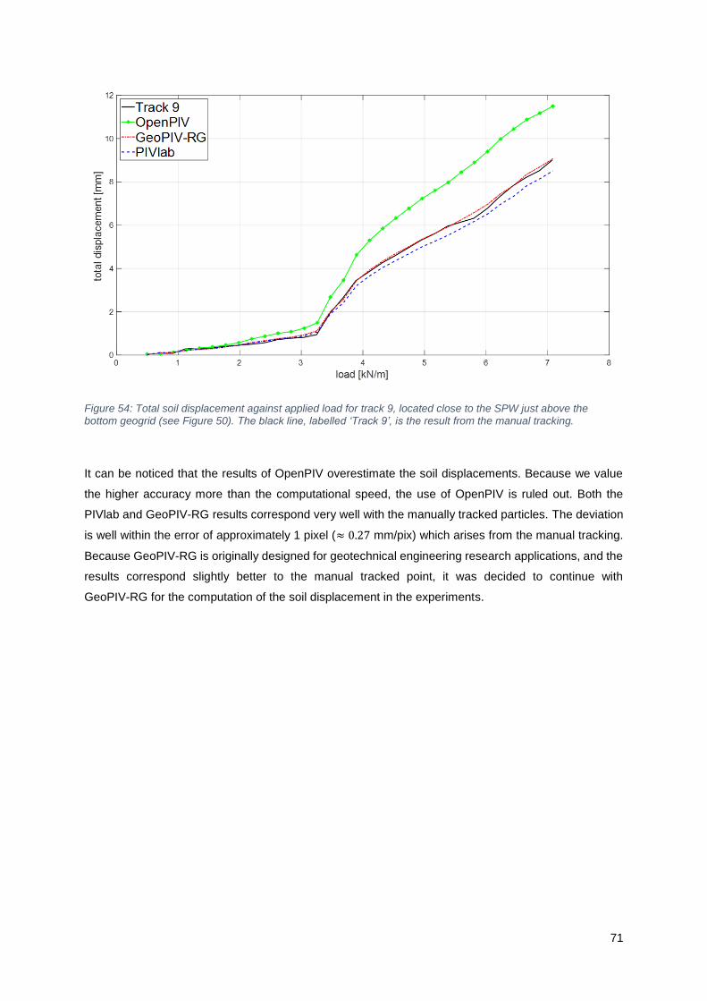
71
Figure 54: Total soil displacement against applied load for track 9, located close to the SPW just above the bottom geogrid (see Figure 50). The black line, labelled ‘Track 9’, is the result from the manual tracking.
It can be noticed that the results of OpenPIV overestimate the soil displacements. Because we value
the higher accuracy more than the computational speed, the use of OpenPIV is ruled out. Both the
PIVlab and GeoPIV-RG results correspond very well with the manually tracked particles. The deviation
is well within the error of approximately 1 pixel (≈ 0.27 mm/pix) which arises from the manual tracking.
Because GeoPIV-RG is originally designed for geotechnical engineering research applications, and the
results correspond slightly better to the manual tracked point, it was decided to continue with
GeoPIV-RG for the computation of the soil displacement in the experiments.

72
8.2.2 Comparison input parameters
The following values of the input parameters were used in previous subsection for the soil displacement
results of GeoPIV-RG:
• an image resolution of 0.27 mm/pix;
• an interrogation window size of 40 pixels;
• an overlapping ratio of 20%, i.e. a spacing of 20 pixels.
In this section, it is first examined whether peak-locking effects are present in the results obtained with
previously used values of the input parameters.
Second, it is examined whether:
1. the original resolution of 0.108 mm/pix leads to higher accuracy;
2. a smaller interrogation window reveals more soil deformation information;
3. the overlapping ratio of 50% leads to bias in the computed strains.
In order to investigate point 1, the GeoPIV-RG soil displacements results for an image resolution of
0.27 mm/pix were compared with an image resolution of 0.108 mm/pix for a similar interrogation window
size in metric units, namely a size of ≈ 10.8 mm·10.8 mm and a spacing of ≈ 5.4 mm. Figure 55 to
Figure 57 compare the resulting soil displacements for point 1, 2 and 4 respectively.
In order to investigate point 2, we compare Figure 59a and Figure 59b. Figure 59a shows the strain
plots obtained with a resolution of 0.108 mm/pix, an interrogation window size of 30 pixels (≈3.2 mm)
and an overlap of 15 pixels. Figure 59b shows the strain plots with a resolution of 0.27 mm/pix, an
interrogation window size of 40 pixels (≈ 10.8 mm·10.8 mm) and a spacing of 20 pixels.
In order to investigate point 3, we compare Figure 59b and Figure 59c. Figure 59b shows the strain plots
obtained with an interrogation window size of 40 pixels and an overlapping ratio of 50% (20 pixels) and
Figure 59c shows a similar window size but a smaller overlapping ratio of 20% (8 pixels).
Initially, it was intended to compare the results with the larger interrogation window size with the results
obtained with a resolution of 0.108 mm/pix and an interrogation window size of 14 mm·14 mm for the
investigation of point 2. This upper limit was required in order to capture the local soil deformations as
explained in Section 8.1.9. However, this analysis turned out to lead to extremely low cross-correlation
coefficients in the order of 10-5 on a scale of -1 to 1, where 0 means no correlation. At larger window
sizes, the information of local deformations would be lost.
The strains are computed according to the definition of ‘linear strains’ also named ‘engineering strains’.
See Appendix B for the calculation procedure of the soil strains in accordance with White and Bolton
(2004).

73
Figure 55: Comparison of total soil displacements obtained from the GeoPIV-RG results with digital test photos as input data with either a resolution of ~0.27 mm/pix or ~0.108 mm/pix. The results are plotted for track 1 (see Figure 50), which location is denoted by the red square in the schematisation of the test set-up included at the bottom right
of this figure.
Figure 56: Comparison of total soil displacements obtained from the GeoPIV-RG results with digital test photos as input data with either a resolution of ~0.27 mm/pix or ~0.108 mm/pix. The results are plotted for track 4 (see Figure 50), which location is denoted by the red square in the schematisation of the test set-up included at the bottom right of this figure.
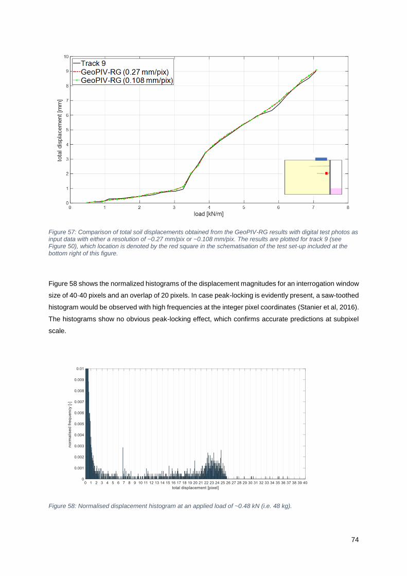
74
Figure 57: Comparison of total soil displacements obtained from the GeoPIV-RG results with digital test photos as input data with either a resolution of ~0.27 mm/pix or ~0.108 mm/pix. The results are plotted for track 9 (see Figure 50), which location is denoted by the red square in the schematisation of the test set-up included at the bottom right of this figure.
Figure 58 shows the normalized histograms of the displacement magnitudes for an interrogation window
size of 40·40 pixels and an overlap of 20 pixels. In case peak-locking is evidently present, a saw-toothed
histogram would be observed with high frequencies at the integer pixel coordinates (Stanier et al, 2016).
The histograms show no obvious peak-locking effect, which confirms accurate predictions at subpixel
scale.
Figure 58: Normalised displacement histogram at an applied load of ~0.48 kN (i.e. 48 kg).

75
Figure 59 shows the total horizontal strain (left), total vertical strain (middle) and total shear strain (right).
The upper row shows the results obtained with a resolution of 0.108 mm/pix, an interrogation window of
30 pixels and overlapping ratio of 50%. The middle row shows the results obtained with a resolution of
0.27 mm/pix, an interrogation window of 40 pixels and overlapping ratio of 50%. The bottom row shows
the results obtained with a resolution of 0.27 mm/pix, an interrogation window of 40 pixels and
overlapping ratio of 20%.
Figure 59: Strain plots (horizontal, vertical and shear strain) generated with different interrogation window size and/or spacing. The upper row (a) shows the results obtained with a resolution of 0.108 mm/pix, an interrogation window of 30 pixels and overlapping ratio of 50%. The middle row (b) shows the results obtained with a resolution of 0.27 mm/pix, an interrogation window of 40 pixels and overlapping ratio of 50%. The bottom row (c) shows the results obtained with a resolution of 0.27 mm/pix, an interrogation window of 40 pixels and overlapping ratio of 20%.

76
The following was noticed from the comparison of (Figure 59a) and (Figure 59b):
• There is no substantial difference between the strain results obtained with the smallest
interrogation window size (3.2 mm) possible compared to the results obtained with an
interrogation window size of 10.8 mm.
• The shear band is less sharp for the results obtained with an interrogation window size of
10.8 mm.
The following was noticed from the comparison of (Figure 59b) and (Figure 59c):
• There is no substantial difference between the strain results obtained with either an overlapping
ratio of 50% or 20%.
• The shear band is less sharp for the results obtained for an overlapping ratio of 20% compared
to the results obtained for an overlapping ratio of 50%.
8.2.3 Conclusions regarding DPIV program and input parameters
From the comparison of the load-displacement curves in section 8.2.1, it is decided to use the DPIV
program GeoPIV-RG for further analyses of the small-scale experiments. The soil displacements agreed
very well with the manually tracked results. The deviation is < 1 pixel (≈ 0.27 mm/pix). Since we assume
high accuracy for the manually tracked points, we also trust the GeoPIV-RG results.
Since no peak-locking effect was observed for the results obtained with an interrogation window size of
40 pixels and a spacing of 20 pixels in Figure 58, the reliability of the results obtained with these input
parameters is ensured.
The following conclusions are drawn concerning the input parameters:
• Since there is no substantial difference between the displacement results obtained with a
resolution of 0.108 mm/pix and the images with 0.27 mm/pix, it was decided to compute the
displacements of the experiments with the 0.27 mm/pix image resolution.
• Also, the benefit of reducing the interrogation window to a size smaller than 40 pixels does not
outweigh the negative effect on the computation time. A drawback is that the slip surface(s) in
the strain plots are less sharp. However, because no more information, i.e. local deformations,
can be retrieved from the figures derived with the smallest interrogation window, we decide to
continue with the reduced size images with an interrogation window of 40 pixels (≈ 10.8
mm·10.8 mm).
• There are no indications of increased accuracy errors due to the use of a too high overlapping
ratio. Therefore, an overlapping ratio of 50% is used to enhance the displacement vector field
and so the sharpness of the slip surface.

77
Attention must be paid to the computation of the strains in the geogrid. It is crucial that the displacement
of the shear band along the geogrid is computed accurately in order to derive reliable strains in the
geogrid. From Figure 59, it can be observed that there were more outliers in the results of the analysis
with a 40 pixels interrogation window size and a resolution of 0.27 mm/pix (Figure 59b) than with the
analysis with the reduced window size and higher resolution (Figure 59a). Since the results with smaller
interrogation window (Figure 59a) did not reduce the amount of outliers compared to (Figure 59b), we
suppose it is a negative consequence of the reduced resolution. In particular close to the SPW, the
accuracy decreased. For the calculation of the strains in the geogrid close to the SPW, it is likely that
an improvement can be obtained with the higher resolution images. Therefore, the images with higher
resolution are used for the derivation of the tensile strain in the geogrid.
8.3 Calculation procedure of the strain in the geogrid
The axial strain in the geogrid is derived in two ways:
1. by making use of the soil displacements obtained with GeoPIV-RG (Stanier et al., 2015);
2. by manually tracking the transverse ribs which were visible on the photos using MTrackJ
(Meijering, n.d.).
8.3.1 Strain in geogrid derived from GeoPIV-RG
In order to derive the strains in the geogrid from the computed soil displacements, we assumed that the
geogrid displacements are equal to the soil displacements close to the geogrid. The underlying
assumption is that we assume a fully rough interface between the geogrid and the grains, such that
𝛿𝑔𝑟𝑖𝑑−𝑠𝑜𝑖𝑙 = 𝜑. Here 𝛿𝑔𝑟𝑖𝑑−𝑠𝑜𝑖𝑙 is the friction angle between soil and geogrid and 𝜑 = the internal friction
angle. In this way, a shear band of soil would develop around the geogrid which displacements can be
computed by means of DPIV.
Figure 60: Assumption for calculation procedure of the strain in the geogrid
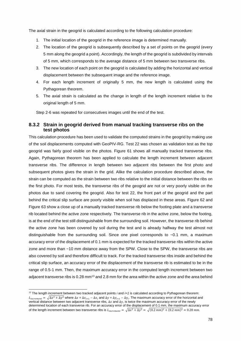
78
The axial strain in the geogrid is calculated according to the following calculation procedure:
1. The initial location of the geogrid in the reference image is determined manually.
2. The location of the geogrid is subsequently described by a set of points on the geogrid (every
5 mm along the geogrid a point). Accordingly, the length of the geogrid is subdivided by intervals
of 5 mm, which corresponds to the average distance of 5 mm between two transverse ribs.
3. The new location of each point on the geogrid is calculated by adding the horizontal and vertical
displacement between the subsequent image and the reference image.
4. For each length increment of originally 5 mm, the new length is calculated using the
Pythagorean theorem.
5. The axial strain is calculated as the change in length of the length increment relative to the
original length of 5 mm.
Step 2-6 was repeated for consecutives images until the end of the test.
8.3.2 Strain in geogrid derived from manual tracking transverse ribs on the test photos
This calculation procedure has been used to validate the computed strains in the geogrid by making use
of the soil displacements computed with GeoPIV-RG. Test 22 was chosen as validation test as the top
geogrid was fairly good visible on the photos. Figure 61 shows all manually tracked transverse ribs.
Again, Pythagorean theorem has been applied to calculate the length increment between adjacent
transverse ribs. The difference in length between two adjacent ribs between the first photo and
subsequent photos gives the strain in the grid. Alike the calculation procedure described above, the
strain can be computed as the strain between two ribs relative to the initial distance between the ribs on
the first photo. For most tests, the transverse ribs of the geogrid are not or very poorly visible on the
photos due to sand covering the geogrid. Also for test 22, the front part of the geogrid and the part
behind the critical slip surface are poorly visible when soil has displaced in these areas. Figure 62 and
Figure 63 show a close up of a manually tracked transverse rib below the footing plate and a transverse
rib located behind the active zone respectively. The transverse rib in the active zone, below the footing,
is at the end of the test still distinguishable from the surrounding soil. However, the transverse rib behind
the active zone has been covered by soil during the test and is already halfway the test almost not
distinguishable from the surrounding soil. Since one pixel corresponds to ~0.1 mm, a maximum
accuracy error of the displacement of 0.1 mm is expected for the tracked transverse ribs within the active
zone and more than ~10 mm distance away from the SPW. Close to the SPW, the transverse ribs are
also covered by soil and therefore difficult to track. For the tracked transverse ribs inside and behind the
critical slip surface, an accuracy error of the displacement of the transverse rib is estimated to be in the
range of 0.5-1 mm. Then, the maximum accuracy error in the computed length increment between two
adjacent transverse ribs is 0.28 mm13 and 2.8 mm for the area within the active zone and the area behind
13 The length increment between two tracked adjacent points i and i+1 is calculated according to Pythagorean theorem:
𝐿𝑖𝑛𝑐𝑟𝑒𝑚𝑒𝑛𝑡 =√∆𝑥2 + ∆𝑦2 where ∆𝑥 = ∆𝑥𝑖+1 − ∆𝑥𝑖 and ∆𝑦 = ∆𝑦𝑖+1 − ∆𝑦𝑖. The maximum accuracy error of the horizontal and
vertical distance between two adjacent transverse ribs, ∆𝑥 and ∆𝑦, is twice the maximum accuracy error of the newly determined location of each transverse rib. For an accuracy error of the displacement of 0.1 mm, the maximum accuracy error
of the length increment between two transverse ribs is 𝐿𝑖𝑛𝑐𝑟𝑒𝑚𝑒𝑛𝑡 =√∆𝑥2 + ∆𝑦2 =√(0.2𝑚𝑚)2 + (0.2𝑚𝑚)2 = 0.28𝑚𝑚.
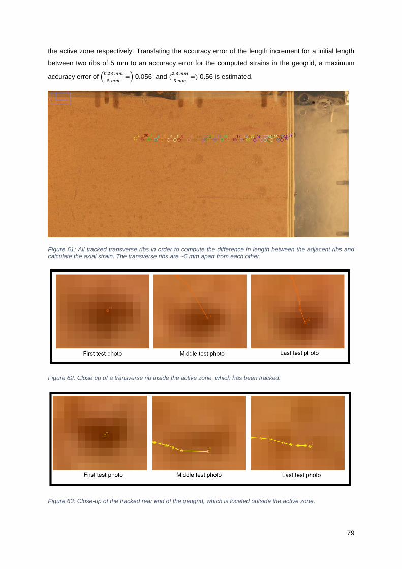
79
the active zone respectively. Translating the accuracy error of the length increment for a initial length
between two ribs of 5 mm to an accuracy error for the computed strains in the geogrid, a maximum
accuracy error of (0.28𝑚𝑚
5𝑚𝑚=) 0.056 and (
2.8𝑚𝑚
5𝑚𝑚=) 0.56 is estimated.
Figure 61: All tracked transverse ribs in order to compute the difference in length between the adjacent ribs and calculate the axial strain. The transverse ribs are ~5 mm apart from each other.
Figure 62: Close up of a transverse rib inside the active zone, which has been tracked.
Figure 63: Close-up of the tracked rear end of the geogrid, which is located outside the active zone.

80
8.3.3 Use of interpolated data to smooth the apparent spiky deformation of the geogrid.
Numerical difference functions are especially sensitive to small variations in the discrete spatial
coordinates describing the location of the geogrid. The displacement of the geogrid is a continuous
function. However, this displacement is described by discrete pixel values. Using a numerical difference
function to estimate the gradients 𝑑𝑥𝑔𝑒𝑜𝑔𝑟𝑖𝑑
𝑑𝑥 and
𝑑𝑦𝑔𝑒𝑜𝑔𝑟𝑖𝑑
𝑑𝑦 by
∆𝑥𝑔𝑒𝑜𝑔𝑟𝑖𝑑
∆𝑥 and
∆𝑦𝑔𝑒𝑜𝑔𝑟𝑖𝑑
∆𝑦 respectively gives an
error. From the horizontal- and vertical spatial coordinates describing the geogrid location, a new set of
cubic spline interpolated coordinates are generated according to (The MathWorks Inc., 2020b). From
the interpolated spatial coordinates, a less spiky, ‘smoothed’, shape of the geogrid is expected. This
shape is ought to be more in accordance with the real deformation of the geogrid. The deformed and
displaced geogrid computed with the raw data is compared and evaluated with the one obtained with
the smoothed data in chapter 7, as well as the results of the axial strains in the geogrid.

81
9 Experimental results and analysis
Chapter 6 gave a description of the test set-up and the test procedure. In addition, Chapter 7 described
boundary effects and Chapter 8 looked at the digital particle image velocimetry that was used to analyse
the results of the experiments. This chapter looks at and analyses the test results. Section 9.1 gives an
overview of the test program. Section 9.2 evaluates the reproducibility of the experiment. Section 9.3
analyses the global failure mechanisms found and looks at the influence of geogrid length, load position
and the number of geogrids on the slip surfaces and deformations. Section 9.4 looks at the influence of
the same aspects on the load-displacement behaviour. Section 9.5 analyses the tensile strain and force
distribution along the geogrid. Hereby, the validity of the four considered PIV-calculation methods has
been investigated. Section 9.6 gives a final analysis of the results out of which conclusions have been
drawn.
9.1 Test program
Table 7 gives an overview of all tests that have been carried out. The tests are sorted per test
configuration.
The following parameters have been investigated:
• length of the geogrid: 6 cm, 11 cm, 13 cm and 18 cm;
• number of geogrids: one or two;
• position of the load: 3 cm, 6 cm, 8.4 cm and 13 cm;
• connection geogrid-SPW: connected or not connected for all tested geogrid lengths.
In total 41 tests have been performed. From these, 28 tests were ‘standard tests’; all with one or two
geogrid anchors while varying the parameters listed above. In addition, some different tests were
performed for comparison reasons. Two of these tests (number 47 and 48) were conducted without any
geogrid anchorage. In nine tests (number 31, 32, 35, 36, 41, 42, 43, 44 and 51), the geogrid was not
connected to the SPW. Finally, a set of five tests was performed to investigate to what extent the part
of the geogrid within the active zone contributes to the total resistance of the geogrid-anchor. For this
purpose, the part of the geogrid within the active zone was removed from an 18 cm geogrid-anchor,
such that only the end part of the geogrid was left. Figure 64 shows a close-up of the ‘half’ geogrid-
anchor. Two steel wires were used to connect the geogrid to the SPW. A 0.5 mm thick brass strip hooks
the geogrid, while the steel wire was pulled through the hook. Three different ratios of the length of the
grid and the wire have been manufactured and tested:
• a ‘half’ geogrid-anchor of which the first 10 cm is a steel wire and the last 8 cm is a geogrid;
• a ‘half’ geogrid-anchor of which the first 13 cm is a steel wire and the last 5 cm is a geogrid;
• a ‘half’ geogrid-anchor of which the first 13 cm is a steel wire and only the brass strip is
attached to it.

82
It is very likely that the brass strip contributes to the total resistance. The last of the three ‘half’ geogrid-
anchor types is included in the test program in order to determine the influence of the brass strip.
Figure 64: 'Half' geogrid-anchor of which the first 10 cm is a steel wire and the last 8 cm geogrid. Note that the geogrid was straightened by pulling a PVD plate across the geogrid before pouring the sand on top.

83
Table 7: Overview of tests
* This test was not used for further analysis
14 The bottom load plate has a thickness of 1.5 cm, a length of 10 cm and a width (in-plane direction of digital test photos) of 9 cm.
Test Number of geogrids, length of geogrid Vertical distance geogrid
[cm from top SPW]
Distance between load plate14 and sheet pile wall
[cm]
Relative density ID [%]
12/13 One; 11 cm 5 3 67 / 71
14/15/26 One; 11 cm 5 6 73/ 74/ 109
16/17/45 One; 18 cm 5 3 68 /74/76
18/19 One; 18 cm 5 13 74 /73
20/21 Two; 18 (top layer) and 11 cm 5 and 12 13 71 /64
22/23
24/25
33/34
Two; 18 (top layer) and 11 cm 5 and 12 3 74 /78
97 /105
66 /67
27/28 One; 6 cm 5 3 92 /81
29/30 One; 6 cm 5 8.4 91 /78
31/32 One; 6 cm; non-connected 5 3 68 /83
35/36 One; 6 cm; non-connected 5 8.4 81 /77
37* No geogrid - 3 67
38/39/40 One; first 10 cm free space + 8 cm grid (‘half’ geogrid-anchor)
5 3 72/75/79
41/42 One; 18 cm; non-connected 5 3 75/76
43/44 One; 11 cm; non-connected 5 3 69/76
46 One; 6 cm; 5 3 68
47 No geogrid - 8.4 75
48 No geogrid - 3 71
49 One; first 13 cm free space + 5 cm grid (‘half’ geogrid-anchor)
5 3 72
50 One; first 13 cm free space + 0 cm grid. (‘half’ geogrid-anchor)
5 3 69
51 One; 13 cm; non-connected 5 3 67
52 One; 13 cm 5 3 65

84
9.2 Reproducibility of the tests
The reproducibility of the experiment has been investigated by comparing the (1) critical slip surface, (2)
soil displacement-load curves and (3) the SPW deformation for tests with one geogrid at 1/6th of the
height of the SPW and the 10 cm loading plate of the load at 3 cm from the SPW:
• three duplicate tests (test 16, 17 and 45) with one geogrid-anchor with a length of 18 cm.
• two duplicate tests (test 12 and 13) with one geogrid-anchor with a length of 11 cm.
9.2.1 Critical slip surface
Figure 65 shows the critical slip surface of the test configuration with one-geogrid anchor of either a
length of 18 cm (left figure) or 11 cm (right figure). The loading plate is positioned 3 cm from the SPW.
Figure 65: Critical slip surfaces (‘planes’) of the test configuration with one geogrid-anchor of either a length of 18 cm (left figure) or 11 cm (right figure).
Figure 65b shows that tests 12 and 13 develop the same 25° straight slip surface. The agreement
between the results of test 16, 17 and 45 in Figure 65a is less, but still reasonable. This figure also
shows the development of the slip surfaces (denoted by ‘1st plane’) during the test, by showing two slip
surfaces for Test 16 and Test 45. First, the development of this straight slip surface was observed. At
continuous displacement of the soil and SPW, a curved slip surface turned out to be dominant. For the
‘1st plane’ an angle of 25° to the vertical is measured. The angle of the critical slip surfaces for Test 12
and Test 13 is equal to 25° also. The ‘straight’ slip surfaces, among which are the 1st slip surfaces15 of
Test 15 and Test 45 and the critical slip surfaces of Test 12 and Test 13 are identical. The critical slip
surfaces of Test 16, Test 17 and Test 45 differ. Test 16 and Test 45 show a more curved slip surface
compared to Test 17.
15 The author uses both ‘plane’ and ‘surface’ to denote the shear bands in the soil.

85
9.2.2 Relation between soil displacement and applied load
Figure 66 gives the total soil displacement as a function of the applied load for three duplicate tests. The
test configuration consists of an 18 cm geogrid-anchor at a depth of 5 cm from the top of the SPW
(1/6th the height of the SPW). The loading plate of the load is positioned 3 cm from the SPW. The
location of the plotted soil displacements is denoted by the red square in the schematization of the
general test-set up. This point in the soil domain is located 13 mm away from the SPW at a depth of
40 mm below ground surface level (50 mm below top SPW). The orange dots indicate the point in time
– and corresponding applied load - at which the full development of the 1st slip surface was observed in
the shear strain colour plots obtained from the DPIV results. It must be noted that the legend chosen of
the shear strain for the output colour plots determines at what point in time the slip surface becomes
clearly visible. The blue dots indicate the point in time when the critical curves slip surface is fully
developed.
Figure 66: Total soil displacement as a function of the applied load for three duplicate tests. The orange dots indicate the magnitude of the applied load at which the full development of the 1st slip surface is observed. The blue dots denote the magnitude of the applied load at which the critical slip surface is fully developed.
The following is observed from Figure 66:
• At a load level < ~3 kN/m, the total displacements between the three tests correspond very well.
• At a load level > 3 kN/m, the total displacements between the three tests deviate significantly.
The maximum difference in soil displacements increases with load level.
• Test 16 and Test 17 show an abrupt increase in displacements at approximately a similar load
level of ~ 3.6 kN/m. However, the displacement continues to increase with a same rate for Test
17, while this rate reduces for Test 16.
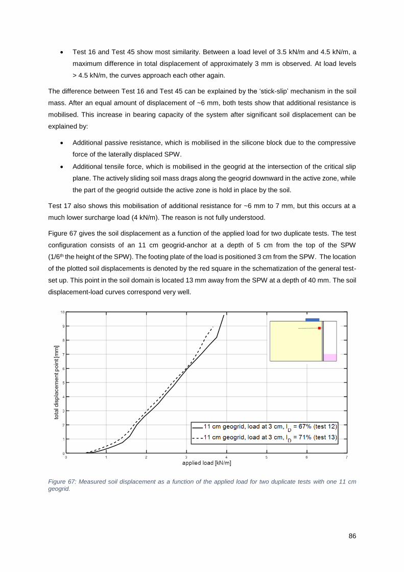
86
• Test 16 and Test 45 show most similarity. Between a load level of 3.5 kN/m and 4.5 kN/m, a
maximum difference in total displacement of approximately 3 mm is observed. At load levels
> 4.5 kN/m, the curves approach each other again.
The difference between Test 16 and Test 45 can be explained by the ‘stick-slip’ mechanism in the soil
mass. After an equal amount of displacement of ~6 mm, both tests show that additional resistance is
mobilised. This increase in bearing capacity of the system after significant soil displacement can be
explained by:
• Additional passive resistance, which is mobilised in the silicone block due to the compressive
force of the laterally displaced SPW.
• Additional tensile force, which is mobilised in the geogrid at the intersection of the critical slip
plane. The actively sliding soil mass drags along the geogrid downward in the active zone, while
the part of the geogrid outside the active zone is hold in place by the soil.
Test 17 also shows this mobilisation of additional resistance for ~6 mm to 7 mm, but this occurs at a
much lower surcharge load (4 kN/m). The reason is not fully understood.
Figure 67 gives the soil displacement as a function of the applied load for two duplicate tests. The test
configuration consists of an 11 cm geogrid-anchor at a depth of 5 cm from the top of the SPW
(1/6th the height of the SPW). The footing plate of the load is positioned 3 cm from the SPW. The location
of the plotted soil displacements is denoted by the red square in the schematization of the general test-
set up. This point in the soil domain is located 13 mm away from the SPW at a depth of 40 mm. The soil
displacement-load curves correspond very well.
Figure 67: Measured soil displacement as a function of the applied load for two duplicate tests with one 11 cm geogrid.

87
9.2.3 SPW displacement
Figure 68 shows the SPW displacement for three duplicate tests at an applied load of 5 kN/m. The SPW
is anchored by a geogrid-anchor of 18 cm length at a depth of 1/6th the height of the SPW. The loading
plate is positioned 3 cm from the SPW. The SPW displacement is derived by automatically tracking
points along the SPW based on the colour contrast of (a black line on) the sealing strip and the
surroundings.
Figure 68: SPW displacement at an applied load of 5.0 kN/m for three duplicate tests (Test 16, 17 and 45) with
one 18 cm geogrid.
From Figure 68, the following is found:
• A maximum difference of ~2 mm displacement between the three tests is observed at the toe
of the SPW.
• Similar SPW displacements are found for Test 17 and Test 45 at the depth of 50 mm, which is
the depth of the point for which the total soil displacement-load curve is plotted in Figure 66.
• The difference in horizontal displacement between the tests reduces towards the top of the
SPW.
The largest lateral SPW displacements are found for Test 17, which corresponds with the test which
shows the largest soil displacements at an applied load of 5 kN/m in Figure 66. However, the similar
SPW displacements for Test 17 and Test 45 at a depth of 50 mm conflicts with the significantly larger
soil displacements at a load level of 5 kN/m in Figure 66. It must be noted that the automatically tracking
calculation procedure does not always result in very accurate SPW displacement results, the results of
the soil displacements are more accurate. This inaccuracy can (partly) explain the unexpected
differences between soil and the SPW displacements.

88
Figure 69 shows the SPW displacement at different load levels for the three duplicate tests.
An abrupt large horizontal displacement of the SPW along the bottom of the box is observed between a
load level of 3 kN/m and 4 kN/m for Test 16 and Test 17, while for Test 45 the sliding is yet to start at a
load level of 4 kN/m. These observations correspond with the load level at which an abrupt increase in
total soil displacement is observed in Figure 66.
Figure 69: SPW displacement at different load levels for three duplicate tests (Test 16, 17 and 45) with one 18 cm geogrid.
Figure 70 shows the SPW displacement for the duplicate tests, Test 12 and Test 13, at a load level of
3.3 kN/m. The SPW is anchored by a geogrid-anchor of 11 cm length at a depth of 1/6th the height of
the SPW. The loading plate is positioned 3 cm from the SPW. The SPW displacement of the duplicate
tests corresponds very well.
Figure 70: SPW displacement at an applied load of 3.3 kN/m for two duplicate tests (Test 12 and Test 13).

89
Figure 71 shows the SPW displacement at different load levels for the duplicate tests Test 12 and Test
13. At all load levels, the SPW displacement agrees very well.
Figure 71: SPW displacement at different load levels for two duplicate tests (Test 12 and Test 13).
9.2.4 Concluding remarks on the reproducibility
Based on the results of the two test configurations, we conclude:
• High reproducibility is achieved with geogrid-anchors having a length < distance between the
SPW and the critical slip surface.
• The reproducibility decreases with increasing displacement of the SPW along the bottom of
the box.
For the test configurations with a geogrid-anchor of 18 cm length, the failure mechanism can be
characterized by a ‘stick-slip’ mechanism. This mechanism is thought to cause most variation between
the duplicate tests. Three factors may contribute to this ‘stick-slip’ mechanism:
• The interaction between geogrid and critical slip surface (shear band) in the soil.
• The friction of the toe of the SPW and silicone block along the bottom of the test box.
• The loading rate may effect the load level at which this stick-slip mechanism occurs.
In Figure 66, a sharp increase in soil displacements is observed at a load between 3.5-4.5 kN/m. In
Figure 69, it can be observed that the SPW abruptly displaces ~5 mm along the bottom of the box at
these load levels. Firstly, the intersection of the critical slip surface with the 18 cm geogrid activates the
part of the geogrid behind the critical surface at a load of ~ 3.9 kN/m and 4.4 kN/m for Test 16 and Test
45 respectively. The additional resistance impedes the sliding of the active soil body. The moment the
driving forces exceed the frictional resisting forces, the geogrid is pulled out. The sharp increase in soil
displacements observed along the curves in Figure 66 at a load between 3.5-4.5 kN/m can be clarified
by this pull-out mechanism at which the soil body starts to slide. Secondly, the reproducibility is largely

90
influenced by the friction of the SPW and silicone block along the bottom of the test box. The larger the
displacement of the SPW along the bottom of the box, the more the friction between the bottom of the
box and SPW plays a role. Although Teflon was installed at the interface SPW-bottom box and silicone
block-bottom box with the purpose of reducing the frictional forces, friction will still be present. Thirdly,
the loading rate may cause the difference in load level at which significant sliding of the soil starts. The
rate at which water was pumped in the bucket, i.e. loading rate, is equal to 0.021 kg/s, 0.020 kg/s and
0.033 kg/s for Test 16, Test 17 and Test 45 respectively. The loading rate affects the strain rate in the
soil. Although strain rate effects for dry soil are found to be negligible at confining pressures ≤ 100 kPa
(Suescun-Florez, Iskander and Bless, 2015), it would explain the similar load level at which slipping
occurs for Test 16 and Test 17 and the higher load level at which slipping occurs for Test 45. Therefore,
it is a parameter which must considered.
Additionally, variations in displacement results are very likely caused by a difference in relative density
between duplicate tests.
9.3 Global failure mechanism
We are interested in the global failure mechanism that develops when the driving forces exceed the
resistance of the geogrid-anchorage.
The aim of this section is to investigate:
• which slip surfaces develop;
• the influence of the position of the surcharge load;
• the influence of the length and number of geogrids.
9.3.1 Development of shear bands: critical and secondary slip surfaces
Initial development of first slip surface and critical slip surface
Figure 72 shows the total shear strain for the test configuration, which consists of an 18 cm geogrid-
anchor. The load plate is positioned 3 cm from the SPW. The shear strain colour plot ranges from a
shear strain of -0.5 (blue), 0 (green) up to 0.5 (red). Two slip surfaces are detected. The number zero
denotes the slip surface, which developed first. The number 1 denotes the critical slip surface which
develops later at a relatively large displacement of the SPW.

91
Figure 72: Total shear strains in Test 16; the test configuration with an 18 cm geogrid-anchor and the loading plate positioned 3 cm from the SPW.
Newly developed critical slip surface at significant overturning of SPW
Figure 73 shows the total shear strain at significant overturning of the SPW. Label ‘0A’ denotes the slip
surface, which developed first. Label ‘1A’ denotes the primary critical slip surface which develops from
the outer edge of the footing plate to the toe of the SPW at relatively large SPW displacement. Label
‘1B’ denotes the secondary slip surface, which initiates at the inner edge of the footing plate and intersect
the SPW – depending on the position of the load - at a depth between 2/5th and 1/2th of the height of
the SPW for a load positioned 3 cm and 13 cm from the SPW respectively. Label ‘2’ denotes the slip
surface, which develops at significant overturning of the SPW. This slip surface develops at the outer
edge of the footing plate and intersects the SPW at the same depth as the secondary slip surface (1B).
Figure 73: a) Total shear strains for test with 18 cm geogrid-anchor at load positioned 13 cm from the SPW (Test 18)
b) Total shear strains for test with 11 cm geogrid-anchor and load positioned 6 cm from the SPW (Test 14)

92
Prandtl failure slip surfaces
Figure 74 shows the total shear strain for four different test configurations. The left two figures give the
shear strain field of the test without geogrid-anchorage and the load positioned either 3 cm (upper left)
or 8.4 cm (lower left) from the SPW. The two figures on the right side give the shear strain field of the
test with a geogrid anchor of 6 cm and the load positioned either 3 cm (upper right) or 8.4 cm
(lower right) from the SPW. In case the load is positioned 8.4 cm from the SPW, the load is entirely
behind the geogrid-anchor. Hence, the normal stress above the geogrid will barely increase due to the
position of the surcharge load.
Figure 74: Total shear strains in Test 28 (upper left figure), Test 48 (lower left figure), Test 30 (upper right figure) and Test 47 (lower right figure).
For all tests in Figure 74, a V-shaped failure mechanism is observed due to the slip surfaces developing
at the inner and outer edge of the loading plate. The slip surface, which initiates at the outer edge of the
loading plate, continues as critical slip surface to the toe of the SPW. The slip surface, which initiates at
the inner edge of the footing, intersects with the critical slip surface or is impeded by the intersection
with the 6 cm geogrid-anchor in Test 30.

93
9.3.2 Influence of the geogrid length
Figure 75 shows the critical slip surfaces for test configurations, which consists of a different length of
geogrid-anchor. The loading plate of 10 cm length is positioned 3 cm from the SPW, such that the outer
edge of the loading plate is 13 cm distance from the SPW.
Figure 75: Comparison between the critical slip surface and the length of the geogrid-anchor. The loading plate is
positioned 3 to 13 cm from the SPW (width of loading plate is 10 cm).
The following is observed from Figure 75:
• All slip surfaces initiate at the outer edge of the loading plate at 13 cm from the SPW.
• A straight slip surface, which intersect the SPW with an angle of 25° to the vertical, is found for
all test configurations.
• The straight slip surface is the critical slip surface for tests without anchorage or a geogrid-
anchor with a length < 18 cm.
• For the test configurations, which consists of a geogrid-anchor with a length of 18 cm (Test 45),
the critical slip surface is curved and wider with respect to the first slip surface.
• All test configurations show a critical slip surface which intersects the SPW at its toe, i.e. at the
bottom of the test box, except for the test without anchorage (Test 48) and the test with the
13 cm geogrid-anchor (Test 52). For these two tests, the critical slip surface intersects the SPW
at ~ 1 cm above its toe. Note that the accuracy of manually tracking the slip surface from the
shear strain results is limited.

94
Figure 76 gives the SPW displacement at different load levels for Test 48 (no anchorage), Test
28 (6 cm geogrid-anchor), Test 12 (11 cm geogrid-anchor), Test 52 (13 cm geogrid-anchor) and
Test 45 (18 cm geogrid-anchor).
The following can be observed from Figure 76:
• For increasing geogrid length (from Test 48 to Test 45), a reduction in SPW displacement is
observed at similar load level. Test 52 (13 cm geogrid-anchor) is an exception for some load
levels.
• Larger SPW displacements are observed for Test 52 (13 cm geogrid-anchor) compared to
Test 12 (11 cm geogrid-anchor) for some load levels.
• The SPW fails by overturning for Test 48 (no anchorage) and Test 28 (6 cm geogrid-anchor).
Sliding of the SPW along the bottom of the box is absent.
• Test 12 (11 cm geogrid-anchor) shows a translational failure mode, but will fail by overturning
at a load level > 2.0 kN/m alike Test 52 (13 cm geogrid-anchor).
• Sliding along the bottom of the box is the dominant deformation of the SPW for Test 45 (18 cm
geogrid-anchor).
Figure 76: SPW displacements at different load levels.
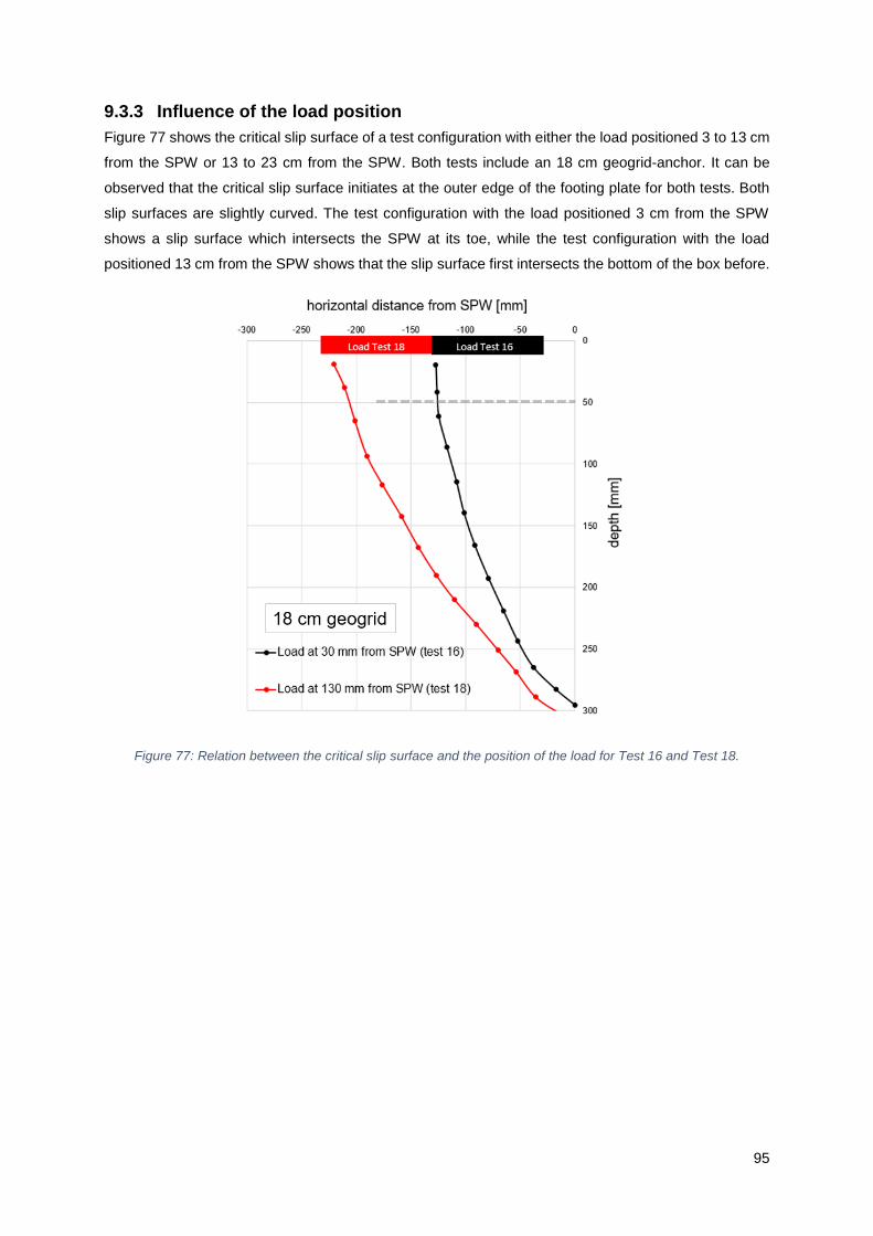
95
9.3.3 Influence of the load position
Figure 77 shows the critical slip surface of a test configuration with either the load positioned 3 to 13 cm
from the SPW or 13 to 23 cm from the SPW. Both tests include an 18 cm geogrid-anchor. It can be
observed that the critical slip surface initiates at the outer edge of the footing plate for both tests. Both
slip surfaces are slightly curved. The test configuration with the load positioned 3 cm from the SPW
shows a slip surface which intersects the SPW at its toe, while the test configuration with the load
positioned 13 cm from the SPW shows that the slip surface first intersects the bottom of the box before.
Figure 77: Relation between the critical slip surface and the position of the load for Test 16 and Test 18.
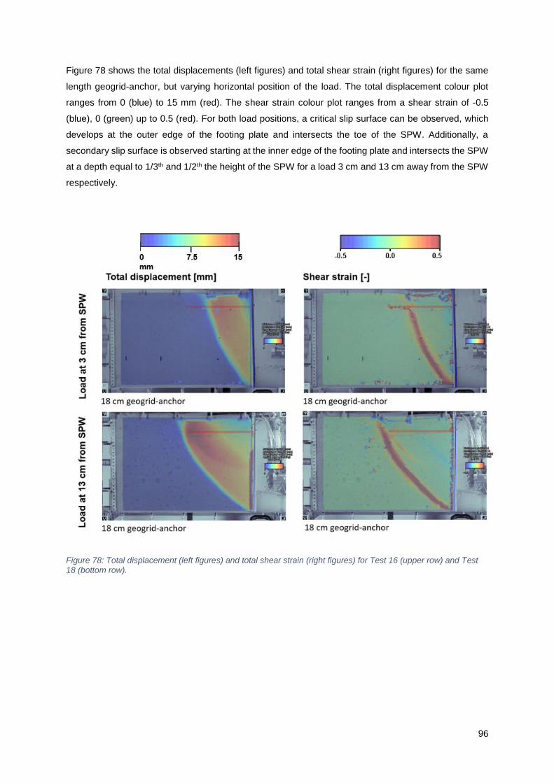
96
Figure 78 shows the total displacements (left figures) and total shear strain (right figures) for the same
length geogrid-anchor, but varying horizontal position of the load. The total displacement colour plot
ranges from 0 (blue) to 15 mm (red). The shear strain colour plot ranges from a shear strain of -0.5
(blue), 0 (green) up to 0.5 (red). For both load positions, a critical slip surface can be observed, which
develops at the outer edge of the footing plate and intersects the toe of the SPW. Additionally, a
secondary slip surface is observed starting at the inner edge of the footing plate and intersects the SPW
at a depth equal to 1/3th and 1/2th the height of the SPW for a load 3 cm and 13 cm away from the SPW
respectively.
Figure 78: Total displacement (left figures) and total shear strain (right figures) for Test 16 (upper row) and Test
18 (bottom row).
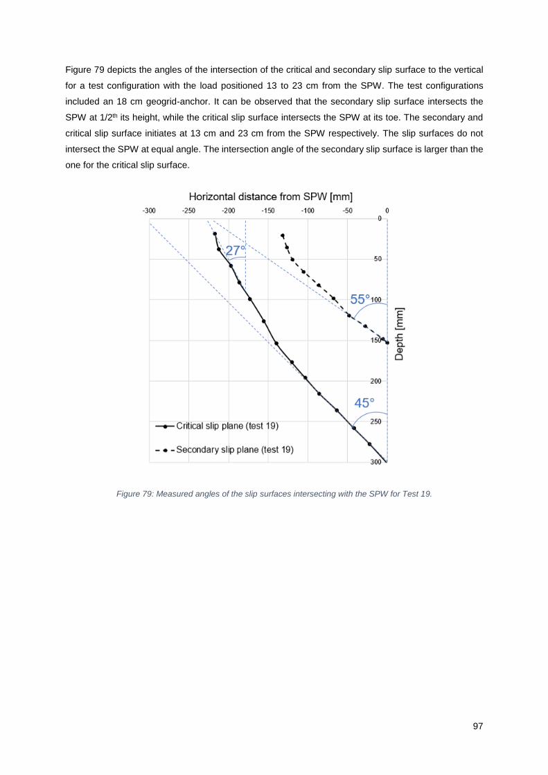
97
Figure 79 depicts the angles of the intersection of the critical and secondary slip surface to the vertical
for a test configuration with the load positioned 13 to 23 cm from the SPW. The test configurations
included an 18 cm geogrid-anchor. It can be observed that the secondary slip surface intersects the
SPW at 1/2th its height, while the critical slip surface intersects the SPW at its toe. The secondary and
critical slip surface initiates at 13 cm and 23 cm from the SPW respectively. The slip surfaces do not
intersect the SPW at equal angle. The intersection angle of the secondary slip surface is larger than the
one for the critical slip surface.
Figure 79: Measured angles of the slip surfaces intersecting with the SPW for Test 19.
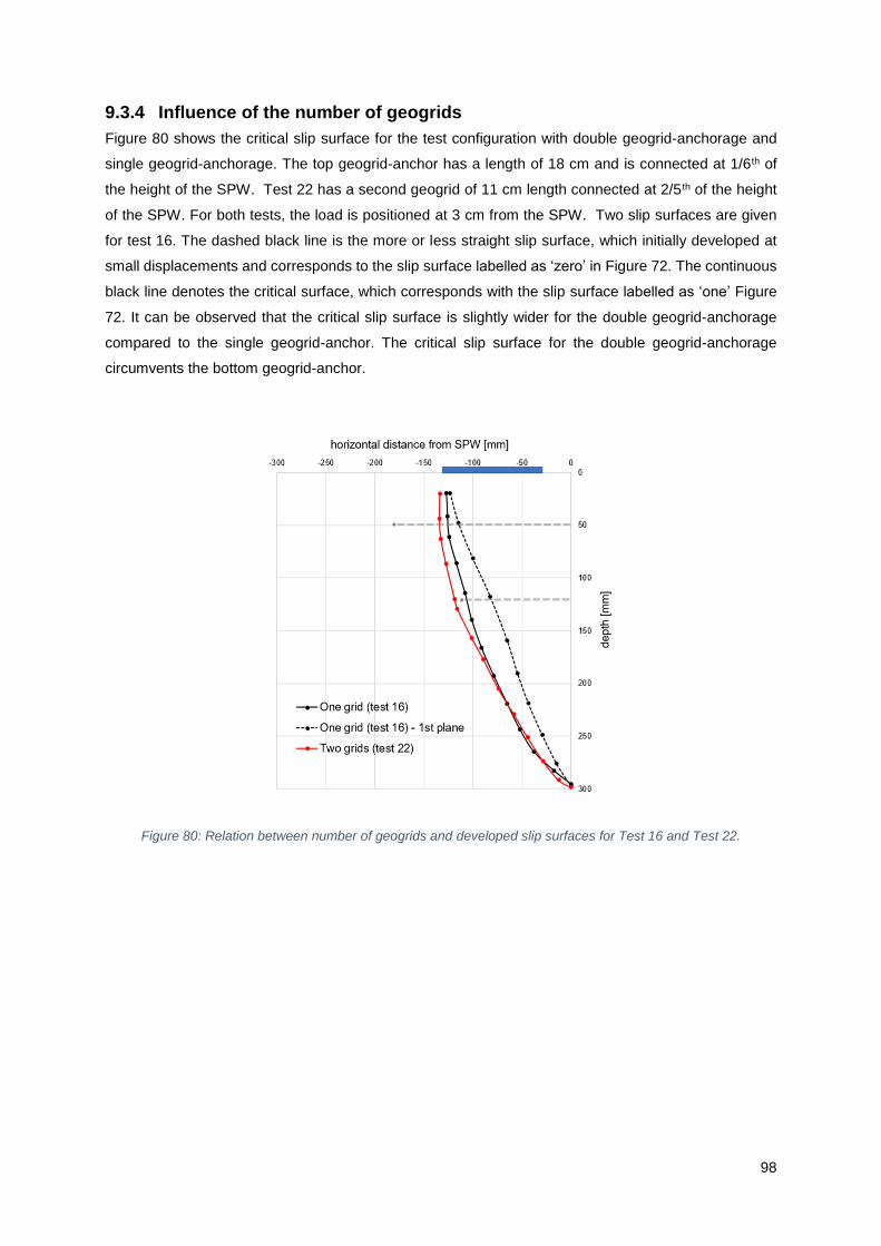
98
9.3.4 Influence of the number of geogrids
Figure 80 shows the critical slip surface for the test configuration with double geogrid-anchorage and
single geogrid-anchorage. The top geogrid-anchor has a length of 18 cm and is connected at 1/6th of
the height of the SPW. Test 22 has a second geogrid of 11 cm length connected at 2/5 th of the height
of the SPW. For both tests, the load is positioned at 3 cm from the SPW. Two slip surfaces are given
for test 16. The dashed black line is the more or less straight slip surface, which initially developed at
small displacements and corresponds to the slip surface labelled as ‘zero’ in Figure 72. The continuous
black line denotes the critical surface, which corresponds with the slip surface labelled as ‘one’ Figure
72. It can be observed that the critical slip surface is slightly wider for the double geogrid-anchorage
compared to the single geogrid-anchor. The critical slip surface for the double geogrid-anchorage
circumvents the bottom geogrid-anchor.
Figure 80: Relation between number of geogrids and developed slip surfaces for Test 16 and Test 22.
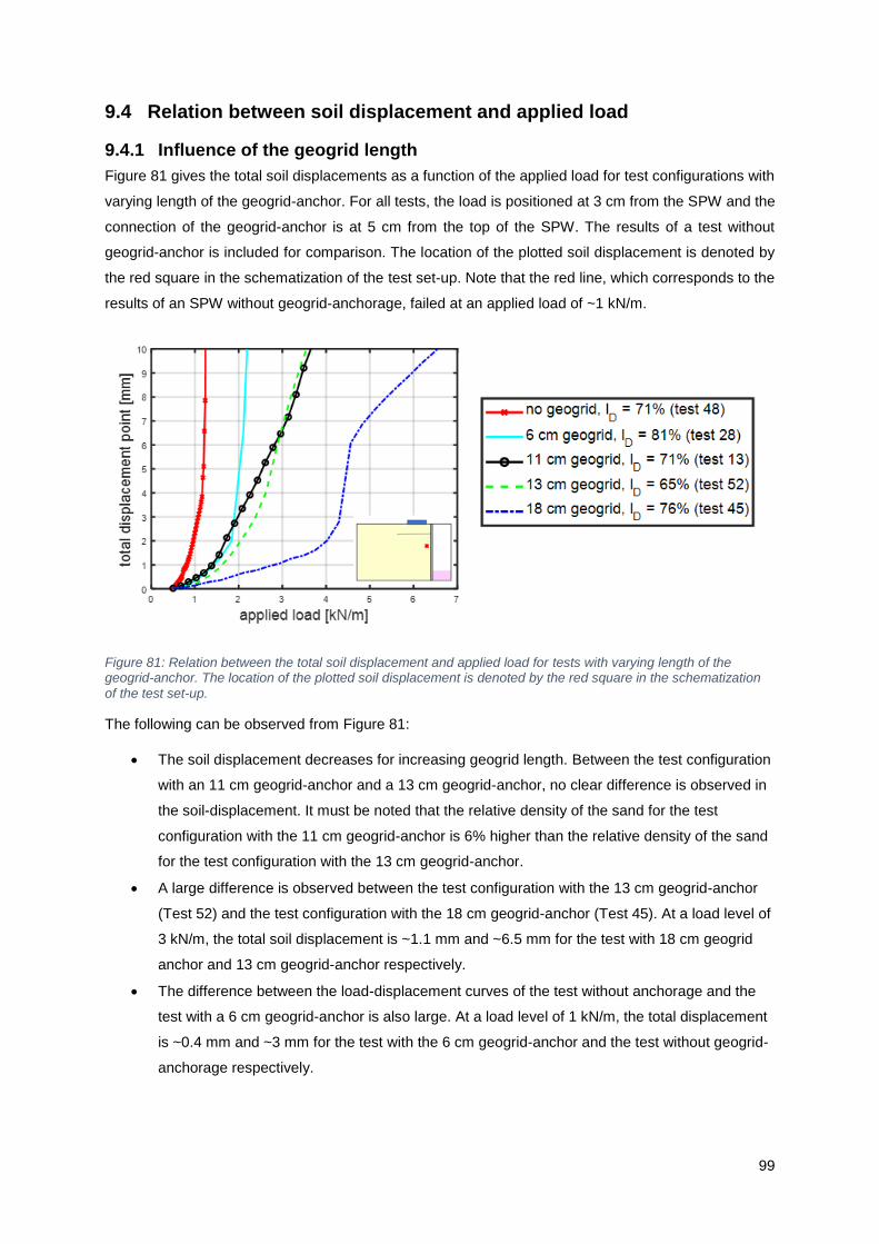
99
9.4 Relation between soil displacement and applied load
9.4.1 Influence of the geogrid length
Figure 81 gives the total soil displacements as a function of the applied load for test configurations with
varying length of the geogrid-anchor. For all tests, the load is positioned at 3 cm from the SPW and the
connection of the geogrid-anchor is at 5 cm from the top of the SPW. The results of a test without
geogrid-anchor is included for comparison. The location of the plotted soil displacement is denoted by
the red square in the schematization of the test set-up. Note that the red line, which corresponds to the
results of an SPW without geogrid-anchorage, failed at an applied load of ~1 kN/m.
Figure 81: Relation between the total soil displacement and applied load for tests with varying length of the geogrid-anchor. The location of the plotted soil displacement is denoted by the red square in the schematization
of the test set-up.
The following can be observed from Figure 81:
• The soil displacement decreases for increasing geogrid length. Between the test configuration
with an 11 cm geogrid-anchor and a 13 cm geogrid-anchor, no clear difference is observed in
the soil-displacement. It must be noted that the relative density of the sand for the test
configuration with the 11 cm geogrid-anchor is 6% higher than the relative density of the sand
for the test configuration with the 13 cm geogrid-anchor.
• A large difference is observed between the test configuration with the 13 cm geogrid-anchor
(Test 52) and the test configuration with the 18 cm geogrid-anchor (Test 45). At a load level of
3 kN/m, the total soil displacement is ~1.1 mm and ~6.5 mm for the test with 18 cm geogrid
anchor and 13 cm geogrid-anchor respectively.
• The difference between the load-displacement curves of the test without anchorage and the
test with a 6 cm geogrid-anchor is also large. At a load level of 1 kN/m, the total displacement
is ~0.4 mm and ~3 mm for the test with the 6 cm geogrid-anchor and the test without geogrid-
anchorage respectively.
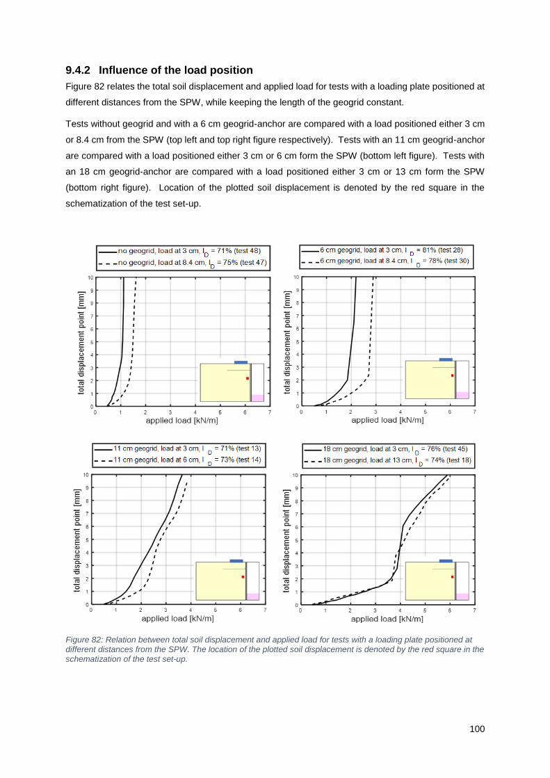
100
9.4.2 Influence of the load position
Figure 82 relates the total soil displacement and applied load for tests with a loading plate positioned at
different distances from the SPW, while keeping the length of the geogrid constant.
Tests without geogrid and with a 6 cm geogrid-anchor are compared with a load positioned either 3 cm
or 8.4 cm from the SPW (top left and top right figure respectively). Tests with an 11 cm geogrid-anchor
are compared with a load positioned either 3 cm or 6 cm form the SPW (bottom left figure). Tests with
an 18 cm geogrid-anchor are compared with a load positioned either 3 cm or 13 cm form the SPW
(bottom right figure). Location of the plotted soil displacement is denoted by the red square in the
schematization of the test set-up.
Figure 82: Relation between total soil displacement and applied load for tests with a loading plate positioned at different distances from the SPW. The location of the plotted soil displacement is denoted by the red square in the schematization of the test set-up.

101
The following can be observed from Figure 82:
• For the tests without anchorage, the failure load is ~25% lower in case the load is positioned
5.3 cm closer to the SPW.
• For the tests with a 6 cm geogrid-anchor, the failure load is 30% lower in case the load is
positioned 5.3 cm closer to the SPW.
• For the tests with an 11 cm geogrid-anchor, a difference of 1 mm to 2 mm in total displacement
at similar load level is observed. A slightly stiffer response is observed when the load is
positioned 3 cm further away from the SPW.
• For the tests with an 18 cm geogrid-anchor, the difference in soil displacement – load curves
due to a different load position is smallest compared to the tests with shorter geogrid-anchorage.
The difference is smallest even if the distance between the load positions is largest.
9.4.3 Influence of the number of geogrids
Figure 83 relates the soil displacement-load curves to the number of geogrid-anchors. The ‘two grids’
results are derived from Test 22, which consists of an 18 cm geogrid-anchor connected at 1/6th of the
height of the SPW and a second geogrid of 11 cm length connected at 2/5th of the height of the SPW.
Test 45 consists of an 18 cm geogrid-anchor connected at 1/6th of the height of the SPW. The location
of the plotted soil displacement is denoted by the red square in the schematization of the test set-up.
Figure 83: Relation between total soil displacement and applied load for tests with a single or double-geogrid anchorage. The location of the plotted soil displacement is denoted by the red square in the schematization of the test set-up.

102
The following is observed from Figure 83:
• Similar load-displacement response is observed at a load level < ~3.2 kN/m.
• An abrupt increase in soil displacement is observed at a load level of ~3.2 kN/m and ~ 4.2 kN/m
for the test with a double geogrid-anchorage (Test 22) and single geogrid-anchorage (Test 45)
respectively.
At load levels > 4.2 kN/m, a stiffer soil response is observed for the test with double geogrid-anchorage
compared to the test with single geogrid-anchorage.
9.4.4 Influence of the geogrid-SPW connection
Figure 84 shows the total soil displacement as a function of the applied load for test configurations by
which the influence of the connection between the geogrid-anchor and SPW is analysed. The location
of the plotted soil displacement is denoted by the red square in the schematization of the test set-up.
Figure 84: Relation between total soil displacement and the influence of the connection between the geogrid-anchor and SPW. The location of the plotted soil displacement is denoted by the red square in the schematization of the test set-up.
The following is observed from Figure 84:
• The soil displacement-load curves for non-connected geogrids with a length < 18 cm are
identical to the soil displacement-load curve for the test without anchorage.
• Lower soil displacements at similar load level are observed for the test configuration with a non-
connected 18 cm geogrid compared to the smaller length non-connected geogrid. Contrary to
the smaller length non-connected geogrids, the non-connected 18 cm geogrid is activated as
the resistance against soil displacement is increased.
• The non-connected 18 cm geogrid show a more or less similar soil displacement-load curve as
the connected 6 cm geogrid-anchor.
• The connection of the geogrid to the SPW leads to significant smaller soil displacements
compared to the non-connected geogrids of similar length.
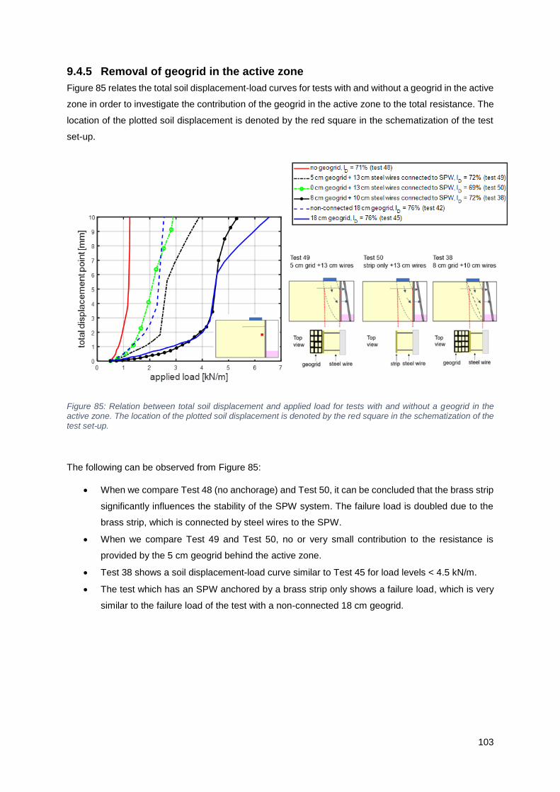
103
9.4.5 Removal of geogrid in the active zone
Figure 85 relates the total soil displacement-load curves for tests with and without a geogrid in the active
zone in order to investigate the contribution of the geogrid in the active zone to the total resistance. The
location of the plotted soil displacement is denoted by the red square in the schematization of the test
set-up.
Figure 85: Relation between total soil displacement and applied load for tests with and without a geogrid in the active zone. The location of the plotted soil displacement is denoted by the red square in the schematization of the test set-up.
The following can be observed from Figure 85:
• When we compare Test 48 (no anchorage) and Test 50, it can be concluded that the brass strip
significantly influences the stability of the SPW system. The failure load is doubled due to the
brass strip, which is connected by steel wires to the SPW.
• When we compare Test 49 and Test 50, no or very small contribution to the resistance is
provided by the 5 cm geogrid behind the active zone.
• Test 38 shows a soil displacement-load curve similar to Test 45 for load levels < 4.5 kN/m.
• The test which has an SPW anchored by a brass strip only shows a failure load, which is very
similar to the failure load of the test with a non-connected 18 cm geogrid.

104
9.5 Tensile force distribution along the geogrid anchorage
The axial strain and tensile force distribution along the geogrid were determined from the measurements
for test 22, which includes a geogrid-anchorage of an 18 cm top geogrid and 11 cm bottom geogrid
connected at 1/6th and 2/5th of the height of the SPW respectively. The loading plate of 10 cm length is
positioned at 3 cm from the SPW.
The axial strain distribution in the top 18 cm geogrid has been determined in two ways:
1. By using the soil displacement results obtained from GeoPIV-RG (Stanier et al., 2015) according
to the calculation procedure described in Section 8.3.1. This section compares the axial strain
distribution in the geogrid obtained with (1) the smoothed spatial coordinates, which describe
the location of the geogrid, and (2) the non-smoothed spatial coordinates.
2. By tracking the transverse ribs of the geogrid manually, which were visible on the photos, using
MTrackJ (Meijering, n.d.). See Section 8.3.2 for more information about the manual tracking
procedure. The strain distribution in the geogrid has been computed for the smoothed and non-
smoothed manually tracked data.

105
9.5.1 Geogrid strains obtained with GeoPIV-RG soil displacements.
This section gives the geogrid strains that were obtained with GeoPIV-RG soil displacements.
Figure 86 shows the deformed top geogrid-anchor of 18 cm at the end of the test. The upper figures
and lower figures show the results of the non-smoothed data and smoothed GeoPIV-RG data
respectively.
Figure 86: Comparison of the final geogrid location determined with non-smoothed vertical coordinates (upper row) and smoothed vertical coordinates (second row). Plots based on results obtained with GeoPIV-RG.
The following can be observed from Figure 86:
• There is no noticeable difference between the geogrid deformation obtained from either the
smoothed or non-smoothed spatial coordinates.
• It can be observed that the geogrid deforms like a kind of hammock. At the front and end part,
the geogrid is held by the SPW and the soil behind the active zone respectively.
• A sharp angle in the deformation is observed at a horizontal position of 0 mm from the original
position of the SPW.
• A maximum vertical displacement of ~10.4 mm is observed at 100 -110 mm from the initial
position of the SPW.

106
Figure 87 gives the horizontal displacement of the rear end of the top 18 cm geogrid-anchor obtained
from the GeoPIV-RG results. No substantial difference can be observed between the results obtained
from the either smoothed or non-smoothed data. According to the results of Figure 87, the geogrid is
pulled out maximally ~ 0.32 mm. At an applied load > 3.3 kN/m, the pull-out displacement reduces again.
The ‘back-pulling’ of the geogrid cannot be true and questions the validity of this GeoPIV-RG calculation
procedure.
Figure 87: Horizontal displacement of rear end of geogrid (pull-out). The result is similar for the smoothed and
non-smoothed data. Plots based on results obtained with GeoPIV-RG.
Figure 88 and Figure 89 give the results of the tensile strain and tensile force along the length of the
geogrid from the (a) non-smoothed spatial coordinates and (b) smoothed spatial coordinates
respectively. The difference between Figure 88 and Figure 89 is the geogrid stiffness (J) of 191 kN/m
(𝑇 = 𝐽 ∙ 휀), where T is the tensile force in the geogrid (kN/m) and 휀 is the geogrid strain (-).

107
Figure 88: Computed strain in top geogrid-anchor of 18 cm length for (a) non-smoothed data and (b) smoothed data. Plots based on results obtained with GeoPIV-RG.
Figure 89: Tensile force along top geogrid-anchor of 18 cm length for (a) non-smoothed data and (b) smoothed
data. Plots based on results obtained with GeoPIV-RG.

108
The following can be observed from Figure 88 and Figure 89:
• Along the length of the geogrid, highest strains – and tensile forces accordingly – are found
close to the SPW and at a distance ~130 mm from the SPW.
• At the rear end of the geogrid, still strain levels of 2% are found, which cannot be accurate.
• At 130 mm from the SPW, strain levels > rupture strain level of 13.48% are observed for the
results obtained from the non-smoothed data and a tensile strain of almost 10% is reached for
the results obtained with the smoothed data.
• Close to the SPW, strain levels > rupture strain level of 13. 48% are found for both the smoothed
and non-smoothed data.
• At a distance of ~30 mm from the SPW, a smaller peak is observed. Tensile strains of ~3.5%
and 4% are observed for the non-smoothed and smoothed data.
• Lowest tensile strains are observed between 40 mm and 100 mm from the SPW. Tensile strains
of 0.8%-1% and ~4 % are observed for the non-smoothed data and smoothed data.
9.5.2 Geogrid strain obtained by tracking transverse ribs manually
This section gives the geogrid strains for Test 22 that were obtained by tracking the transverse ribs
manually.
Figure 90 shows the deformed top geogrid-anchor of 18 cm at the end of the test. The deformation is
derived from the manually tracked transverse ribs of the geogrid. Results are given for (a) the non-
smoothed spatial coordinates and (b) smoothed spatial coordinates.
Figure 90: Final location of geogrid for (a) non-smoothed and (b) smoothed data. Plots based on manually tracked results.

109
The following can be observed from Figure 90:
• Indeed, a more smoothed deformed geogrid is observed from the smoothed spatial coordinates
compared to the non-smoothed spatial coordinates. For example, at a distance of 95 mm from
the initial position of the SPW, i.e. a horizontal distance of 0 mm, the geogrid makes a sharp
angle in Figure 90a compared to Figure 90b.
• For both the smoothed and non-smoothed results, a maximum vertical displacement of ~10.4
mm is observed.
Figure 91 gives the horizontal displacement of the rear end of the top 18 cm geogrid-anchor obtained
from the manual tracking results. A similar trend is observed between the results obtained from
either the smoothed or non-smoothed data. Due to the smoothing, the final pull-out displacement
has increased by 0.2 mm. The rear end has been pulled out 5.4 mm to 5.6 mm at the end of the
test.
Figure 91: Pull-out of geogrid for (a) non-smoothed and (b) smoothed data. Plots based on manually tracked results.
Figure 92 and Figure 93 give the results of the tensile strain and tensile force along the length of the
geogrid from the (a) non-smoothed spatial coordinates and (b) smoothed spatial coordinates
respectively.
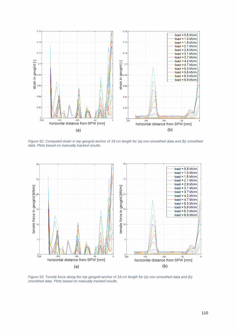
110
Figure 92: Computed strain in top geogrid-anchor of 18 cm length for (a) non-smoothed data and (b) smoothed data. Plots based on manually tracked results.
Figure 93: Tensile force along the top geogrid-anchor of 18 cm length for (a) non-smoothed data and (b)
smoothed data. Plots based on manually tracked results.

111
The following has been observed from Figure 92 and Figure 93:
• The tensile strain and tensile force results of the non-smoothed data is very spiky compared to
the results of the smoothed-data, which shows a similar distribution as the results derived from
GeoPIV-RG.
• Close to the SPW and at ~130 mm distance from the SPW, a tensile strain of 9.5% is observed
from the results of the smoothed data set.
• From the smoothed data set, tensile strains of ~0.4% are observed between 40 mm and 110 mm
from the SPW and again at a distance > ~150 mm from the SPW.
9.5.3 Comparison displacement of geogrid and soil displacement
In order to get more insight into the difference between the displacement of the geogrid and the soil
displacements around the geogrid, the displacement versus applied load have been plotted for a
manually tracked transverse rib and the soil displacements at that location. For the soil displacements,
soil subsets of 5 mm by 5 mm were automatically tracked by means of GeoPIV-RG.
Figure 95 to Figure 98 show the total displacement results for point 3, 5, 8, and 12 (see Figure 94),
which are located on a transverse rib of the upper geogrid from the front to the rear end respectively.
Figure 94: Manually tracked points: both transverse ribs are tracked as well as soil particles just above or below the transverse rib in order to compare the displacements.

112
Figure 95: Total displacement of point 3 in Figure 94, a transverse rib located 1.8 cm from the front-end of the
geogrid, which corresponds to 1/10th of the total length.
Figure 96: Total displacement of point 5 in Figure 94, a transverse rib located 7 cm from the front-end of the geogrid, which corresponds to approximately 2/5th of the total length.

113
Figure 97: Total displacement of point 8 in Figure 94, a transverse rib located 10.5 cm from the front-end of the geogrid, which corresponds to 3/5th of the total length.
Figure 98: Total displacement of point 12 in Figure 94, a transverse rib located 17 cm from the front-end of the geogrid, which corresponds to 17/18th of the total length.

114
The following can be observed from Figure 95 to Figure 98:
• For point 3, the soil displacements differ less than 0.5 mm between the manually tracked
transverse rib and GeoPIV-RG soil displacements results.
• For point 5, the soil displacements match the displacement of the manually tracked rib very well.
• For point 8, the soil displacements differ less than 1 mm between the manually tracked
transverse rib and GeoPIV-RG soil displacements.
• For point 12, the total displacement of the transverse rib differs at the end of the test more than
6 mm larger than the nearby soil displacement computed by GeoPIV-RG.
From those four tracked transverse ribs, the average axial strain between the ribs can be calculated.
Table shows the results at an applied load of 6 kN/m. The average axial strain (휀)̅ has been calculation
according to the following equation:
휀 ̅ = ∆𝑙
𝑙0∙ 100% (9.1)
Table 8: Average axial strains in 18 cm geogrid.
Point Original distance between ribs (𝑙0)
[mm]
Total displacement
[mm]
Stretch between ribs (∆𝑙)
[mm]
Average axial strain between ribs (휀)̅
[%]
3 - 4.2 -
5 52 7.9 3.7 7.1note16
8 35 8.4 0.5 1.4note17
12 65 5.1 3.3 5note18
The manually calculated average strains between the tracked ribs show strains which are smaller than
the strain at rupture. This finding agrees with the observations after the experiments for which no rupture
of the geogrid was noticed. However, we would expect to see plastic deformation of the geogrid at the
end of the experiment if strains of 7.1% would have occurred. In agreement with Figure 92b, higher
average strains are computed close the to the SPW (between point 3 and 5) and along the length which
captures the intersection with the critical slip surface (between point 8 and 12) relative to the average
strain along the length of the geogrid at a distance of 70 to 105 mm from the SPW (between point 5 and
8).
note16 Average strain between point 3 and point 5. note17 Average strain between point 5 and point 8. note18 Average strain between point 8 and point 12.
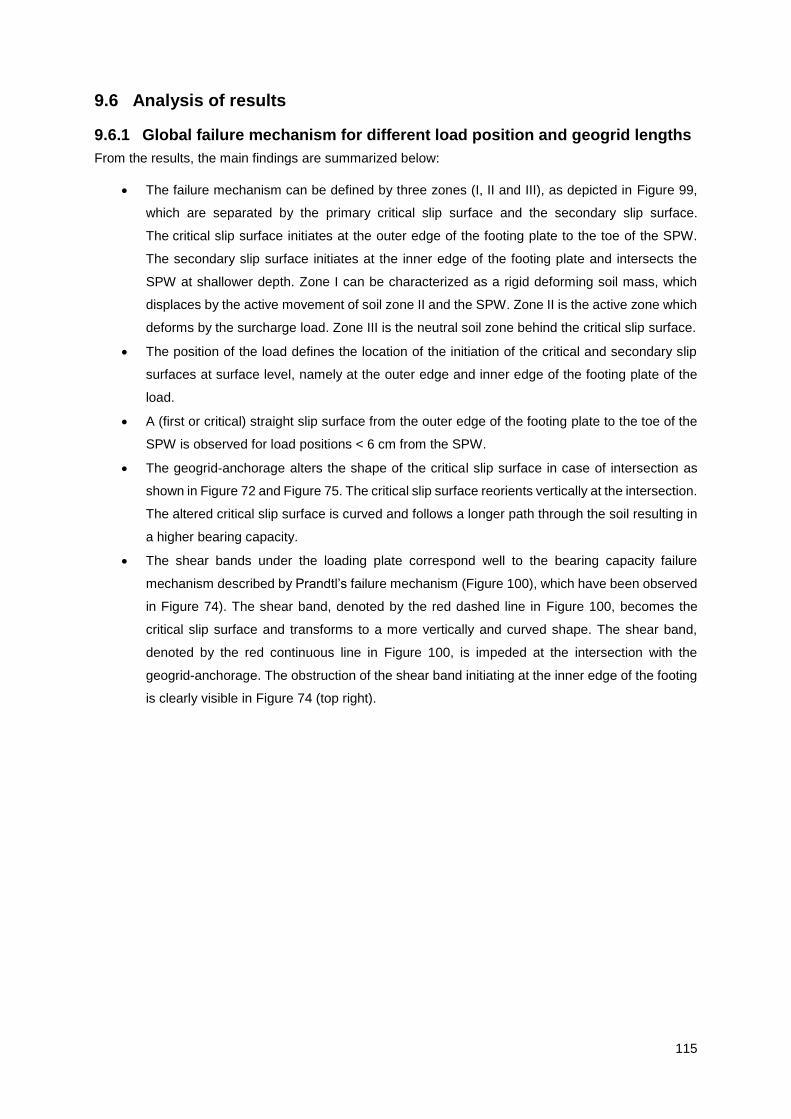
115
9.6 Analysis of results
9.6.1 Global failure mechanism for different load position and geogrid lengths
From the results, the main findings are summarized below:
• The failure mechanism can be defined by three zones (I, II and III), as depicted in Figure 99,
which are separated by the primary critical slip surface and the secondary slip surface.
The critical slip surface initiates at the outer edge of the footing plate to the toe of the SPW.
The secondary slip surface initiates at the inner edge of the footing plate and intersects the
SPW at shallower depth. Zone I can be characterized as a rigid deforming soil mass, which
displaces by the active movement of soil zone II and the SPW. Zone II is the active zone which
deforms by the surcharge load. Zone III is the neutral soil zone behind the critical slip surface.
• The position of the load defines the location of the initiation of the critical and secondary slip
surfaces at surface level, namely at the outer edge and inner edge of the footing plate of the
load.
• A (first or critical) straight slip surface from the outer edge of the footing plate to the toe of the
SPW is observed for load positions < 6 cm from the SPW.
• The geogrid-anchorage alters the shape of the critical slip surface in case of intersection as
shown in Figure 72 and Figure 75. The critical slip surface reorients vertically at the intersection.
The altered critical slip surface is curved and follows a longer path through the soil resulting in
a higher bearing capacity.
• The shear bands under the loading plate correspond well to the bearing capacity failure
mechanism described by Prandtl’s failure mechanism (Figure 100), which have been observed
in Figure 74). The shear band, denoted by the red dashed line in Figure 100, becomes the
critical slip surface and transforms to a more vertically and curved shape. The shear band,
denoted by the red continuous line in Figure 100, is impeded at the intersection with the
geogrid-anchorage. The obstruction of the shear band initiating at the inner edge of the footing
is clearly visible in Figure 74 (top right).
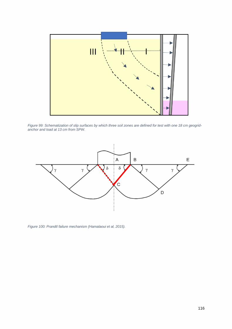
116
Figure 99: Schematization of slip surfaces by which three soil zones are defined for test with one 18 cm geogrid-anchor and load at 13 cm from SPW.
Figure 100: Prandtl failure mechanism (Hamalaoui et al, 2015).

117
9.6.2 Relation between soil displacement and applied load
The main findings are summarized below:
• Based on the results of Figure 81, a clear relation is found between the length of the geogrid-
anchor and the maximum load reached; the longer the geogrid, the higher the bearing capacity.
No increase in load at a particular soil displacement is observed between the results for an
11 cm geogrid-anchor and 13 cm geogrid-anchor. The 2 cm longer geogrid will very likely
counterbalance the lower shear strength due to the 6% lower relative density of the sand.
• From Figure 82, it can be found that the benefits of the relatively large distance between the
loading plate and SPW become smaller for increasing geogrid length. Several factors are
influencing the stability of the system:
a) Comparing the results of the tests without anchorage, a stiffer soil response is
observed in case the load is positioned further away from the SPW. When the load is
further away from the SPW, the length of the slip surface increases and accordingly
the soil resistance along the slip surface. In addition, this position gives a favourable
distribution of the load (further away from the SPW).
b) Comparing the results of the 6 cm geogrid-anchorage, a similar relation is found as for
the tests without anchorage. Clearly, the increased length of the critical slip surface is
more beneficiary regarding the total resistance than the increase of normal pressures
above the geogrid-anchorage, which would be the case if the load is positioned close
to the SPW above the 6 cm geogrid.
c) Comparing the results of the tests with an 18 cm geogrid-anchorages, no substantial
difference is observed between the two load positions. When the load is positioned
13 cm from the SPW, there is a benefit of increased length of the slip surface and a
favourable distribution of the load. When the load is positioned 3 cm from the SPW,
the 18 cm geogrid will increase the soil resistance at the intersection with the critical
slip surface and will benefit from the resistance of the part of the geogrid outside the
active zone. Apparently, these factors counterbalance each other, which results into
the same soil response at a given load.
• From Figure 83, the soil response between one 18 cm geogrid-anchor and the two-geogrid
anchorage is similar at small soil displacements (<1 mm). At larger soil displacements, the two-
geogrid-anchorage system shows a stiffer soil response. Probably, additional tensile force is
mobilised in the geogrids at the intersection with the critical slip surface, when the soil in the
active zone starts to slide as one mass along the slip surface. In case of two geogrids, both
intersecting the slip surface, more resistance against sliding will be delivered.
• From Figure 84, it can be concluded that the part of the geogrid inside the active zone does not
provide any resistance when there is no connection with the SPW.
• From Figure 84, it can be concluded that the total bearing capacity of the system is increased
by 50-65% due to the connection of the geogrid with the SPW. This contribution is determined
for total soil displacements < 3 mm, which is before significant sliding of the active soil body.

118
• From Figure 85, it is observed that equal resistance is provide by the 18 cm geogrid-anchor
(Test 45) and the half’ geogrid-anchor of which the first 10 cm is a steel wire and the last 8 cm
is a geogrid (Test 38) for load levels < ~4.5 kN/m. After the abrupt large soil displacements,
which represent the sliding soil body in the active zone (zone II in Figure 99), additional
resistance is mobilised by the 18 cm geogrid-anchor. Apparently, the part of the geogrid in the
active zone close to the SPW is activated and provides the additional resistance. Since no
additional resistance is mobilised after large soil displacements for the test configuration with
a non-connected 18 cm geogrid (Test 42), it can be concluded that the connection of the
geogrid to the SPW is required for the mobilisation of additional resistance by the geogrid in
the active zone.
9.6.3 Tensile force distribution along the geogrid anchorage
Before analysing the results of the strain and tensile force in the geogrid, the influence of smoothing the
data is discussed first. From Figure 86 and Figure 90, it can be concluded that smoothing the spatial
coordinates do not affect the total vertical displacement of the geogrid. It does also not result into a
substantial different deformation pattern. Only the spikes in the deformation are smoothed out, which
was our intention of this post-processing technique, as explained in Section 8.3.3. Concludingly,
‘smoothing’ the spatial coordinates does not substantially change the deformation pattern of the geogrid,
but significantly affects the computed strain in the geogrid.
The results of the strain and tensile force in the geogrid show spurious high values at the front and end
part of the geogrid. Axial strains of 13.48% are computed, which is larger the maximal strain at rupture
of the geogrid. It is highly unlikely that such high strains developed in the geogrid during the test as no
plastic deformation was measured afterwards. The unrealistic high geogrid strains at the connection
with the SPW is a result of inaccurate DPIV data close to the SPW. Soil particles covering the transverse
ribs close to the SPW, made it also impossible to track the ribs in an accurate way manually.
The strain results in the geogrid obtained with the GeoPIV-RG data also resulted in spurious high strains
in the part of the geogrid that lies outside the active zone. These high strains are clarified by Figure 87
and Figure 96. These figures show that the soil displacements derived with GeoPIV-RG do not
correspond with the displacement of the geogrid. The underestimated geogrid displacements result in
apparent high strains in the geogrid.
The strains and tensile forces derived from the smoothed displacement of the manually tracked ribs of
the geogrid, which are given by Figure 92b and Figure 93b, are considered most reliable. Between the
peaks, a strain of 0.004-0.005 is computed. This corresponds to a tensile force of 0.76-0.95 kN/m for an
axial stiffness of 191 kN/m (Section 6.1.2). Although the two peaks show unrealistic high values, the
build-up of strain at these locations is very plausible considering the deformation of the geogrid shown
in Figure 90. The geogrid-anchor is pushed downward together with the soil in the active zone due to
the surcharge load. Here, the active zone is defined as the zone enclosed by the secondary and critical
slip surface, as denoted by ‘zone II’ in Figure 99. Because the geogrid is connected to the SPW on one
side and hold in place on the other side (partly) by the soil outside the active zone, the geogrid will very

119
likely be stretched close to the SPW and at the location of the critical slip surface. This is in accordance
with the deformation pattern of the geogrid shown in Figure 99.
Based on the measured strains and soil displacement-load curves, the dominant interaction
mechanisms seem to be:
• The transfer of vertical soil stresses via the geogrid to the SPW, which is depicted in Figure
101a.
• The increase of resisting shear stresses along the slip surfaces due to shearing between the
soil and geogrid. The mobilised tensile force in the geogrid, acting across the plane of maximum
stress obliquity in the soil, reduces the soil shear force along the slip surface and increases the
normal force in the soil. This mechanism is depicted in Figure 101b. As a result, the slip surface
changed in shape at the intersection with the geogrid layers, resulting in an increase of the
length of the slip surface and an increase in bearing capacity.
Figure 101: Dominant interaction mechanisms: (a) transfer of vertical soil stresses via the geogrid to the SPW and (b) increase of resisting shear stresses along the slip surfaces due to shearing between the soil and geogrid.
120
10 Numerical model of the small-scale experiments
This chapter presents a numerical model of the small-scale experiment. Section 10.1 describes the
model and gives an overview of the input parameters. Section 10.2 explains how the numerical model
is manipulated such that the influence of the sidewall friction in the small-scale experiment is included
in the plane strain numerical model. The validity of the methodology used is examined using analytical
formulations for the stress reduction due to sidewall friction (Jewell, 1987). Section 10.3 concerns the
bottom boundary conditions of the model. Three models with different bottom boundaries are compared
and the one that fits the small-scale experimental results best is chosen as final model. Chapter 11
presents and analyses the results of the numerical model.
10.1 Description of the model
The small-scale 1g physical experiment is simulated by a 2D (plane strain) finite element numerical
model for which the software PLAXIS 2D 2019 is utilized (Plaxis bv., 2019).
10.1.1 Boundary conditions
The dimensions of the model are identical to the small-scale experiment except for the depth. Due to a
mistake, the surface level of the soil is one centimetre higher (30 cm instead of 29 cm). Since the
reduced weight (see Section 10.2) of the soil is small relative to the surcharge load, no significant
differences in results will be obtained.
The bottom of the test box is modelled in order to include the frictional components between the bottom
of the box and the soil, SPW and silicone block. Section 10.3 looks at the bottom boundary conditions.
At the left and right boundaries of the model, horizontal displacement is restrained. At the top boundary,
free displacement is allowed.
10.1.2 Mesh
A mesh is generated using six-node triangular elements. 6 -Node elements are preferred above
15 node-elements, because sharper shear bands in the soil can be computed. When 6-node elements
are used, four times more elements can be applied at similar computational costs. Since the 6-node
elements will be consequently four times smaller, less distortion of the element shape occurs and
sharper shear bands can be computed with the smaller elements. However, care must be taken. Plaxis
bv. (2019) warns that lower accuracy is obtained with 6-node elements compared to 15-node elements,
because of the lower order of interpolation and lower number of numerical integration points (stress
points). In situations where failure plays a role, failure loads are generally overpredicted using 6-noded
elements (Plaxis bv., 2019).
A medium size mesh is applied with mesh refinement at areas where high strains occur. The model is
built up out of 22195 elements and 45967 nodes.

121
10.1.3 Phases
The preparation phase of the small-scale experiment is simulated in the numerical model with 8 phases.
This way, it is tried to obtain an initial stress state which corresponds to the stress state at the start of
the experiment. Figure 102 shows the 8 phases before applying the surcharge load on the footing plate.
The load is simulated by prescribing a vertical displacement pointing downward at the centre of the
footing plate. During these 8 phases, the SPW is fixed with a fixed-end anchor with an axial stiffness
(EA) of 5500 kN that is placed at 1 cm below the top of the SPW. This fixed-end anchor models the
uPVC plate, which is placed between the SPW and front wall of the test box. The uPVC is hold in place
by a clamp. The axial stiffness of the fixed-end anchor is estimated on the axial stiffness of the uPVC
plate and the axial stiffness of the front wall. Phases 7 and 8 are reversed with respect to the preparation
procedure of the small-scale experiment. In the small-scale experiment, the footing plate with the bucket
on top are placed first before the sheet pile is set free. As a result, the small-scale experiment starts
with an initial load of ~5 kg, which corresponds to 0.5 kN/m. No deviations are expected between the
experimental and numerical soil displacements at loads > 0.5 kN/m due to this phase swap.
Figure 102: Build-up of numerical model. Stage 1 to 6 are the preparation phases. The sheet pile was set free in phase 7. Phase 8 installs the footing plate. During the phases that follow, a vertical soil displacement is prescribed at the centre of the footing plate, which pushes the plate downward.
10.1.4 Modelling the soil
The hardening soil (HS) model is applied to model the behaviour of the Baskarp B15 sand behind the
SPW.
Results of drained consolidated triaxial tests for Baskarp B15 with a relative density of ~ 80% (Ibsen,
2009) are used to determine the values of the soil strength and stiffness parameters adjusted for (a) the
confining pressure in the small-scale experiment and (b) plane strain conditions. The strength of the soil
is described by the cohesion (c), secant internal friction angle (𝜑) and dilatancy angle (𝜓). The confining
pressure ranges between 5 and <70 kPa. For this range of confining pressures, 𝜑𝑡𝑟 ranges between
42° and 55° and the internal friction angle at critical state 𝜑𝑐𝑣 is determined equal to 34°. Correcting for

122
plane strain conditions, using equation 10.1 which is derived from Bolton’s large database, a plane
strain internal friction angle 𝜑𝑝𝑠 ranging between 47° and 58° is found (Bolton (1986).
𝜑𝑝𝑠 =5
3𝜑𝑝𝑡𝑟 −
2
3𝜑𝑐𝑣 (10.1)
Because the high 𝜑𝑝𝑠 are disputable, it is chosen to use an internal friction angle of 45° for the numerical
model. The corresponding dilatancy angle is determined based on Rowe’s equation (Rowe, 1962):
𝑠𝑖𝑛𝜓 = sin𝜑−𝑠𝑖𝑛𝜑𝑐𝑣
1−𝑠𝑖𝑛𝜑𝑠𝑖𝑛𝜑𝑐𝑣 (10.2)
A dilatancy angle of 14° is determined and used for the numerical model. The cohesion is directly derived
from the triaxial tests and is equal to 0.6 kPa (Deltares, 2019). The stiffness of the soil is described by
the secant Young’s modulus from the triaxial tests 𝐸50𝑡𝑟 and the Poisson ratio. The stress-dependency of
the stiffness parameters is described by the power index m according to equation 10.3:
𝑚 =ln(
𝐸50𝑟𝑒𝑓
𝐸50)
ln(𝜎3𝑟𝑒𝑓
𝜎3)
(10.3)
From the triaxial tests, 𝐸50𝑟𝑒𝑓
is determined to be 72.4 MPa at a reference confining pressure of 100 kPa
and m = 0.54. The Poisson ratio is determined to be 0.25. In order to take account of the preparation
procedure during which the soil was simultaneously poured in the test box and densified up to surface
level, a higher lateral earth pressure coefficient 𝐾0 at initial stress state is used compared to the one that
would be derived from Rankine’s theorem (𝐾0 = 1 − 𝑠𝑖𝑛𝜑). Accordingly, 𝐾0 is estimated to be equal to
0.5.
10.1.5 Modelling the geogrid
The geogrid is modelled as a geogrid element with two translational degrees of freedom, namely
horizontal and vertical displacement (Plaxis bv., 2019). The connection of the geogrid with the SPW is
simply described by a mutual node. The behaviour of the geogrid is described by the axial stiffness. It
does not have a bending stiffness. The axial stiffness of the geogrid is derived directly from tensile tests
(Kloster, 2016). The short-term stiffness equal to 191 kN/m (Section 6.1.2) at an axial strain of 2% is
chosen as input parameter, because the test duration is less than an hour and no higher axial strains
than 2% are expected in the small-scale experiment19. The underlying assumption is that the stiffness
response of the geogrid is similar in the tensile tests as in the small-scale experiment. Whether this
assumption is valid, depends on several factors.
19 Culmann’s method – among others described in CUR198 (2017) is applied to estimate the tensile force in the geogrid at a maximum load of 6 kN/m. A straight slip surface from the outer edge of the footing plate – positioned 3 cm from the SPW- and the toe of the SPW is assumed. The area bounded by the SPW and slip surface forms a triangular wedge for which force equilibrium is assumed. Hereby, the passive force is estimated to be 0.08 kN/m (assuming 1% compression of the silicone block), the weight of the soil wedge is estimated by the area of the triangular wedge times the volumetric weight of the soil (𝛾 =
16.3𝑘𝑁
𝑚3). The direction of the resisting shear forces is described by the angle 𝜑 with the normal of the slip surface. Then, the
tensile force in the geogrid can be estimated based on horizontal force equilibrium. The tensile force is estimated to be 2.4 kN/m. At tensile forces < 4 kN/m, the axial strain is < 2% (Kloster, 2016).

123
Moraci et al. (2014) states that the tensile strength obtained by in air tests in pullout conditions is very
close to the tensile strength obtained in pullout conditions at the same rate of displacement. The rate of
displacement was (21.2%/min of 58.54 mm = ) 12.4mm/min during the tensile tests. Farrag et al. (1993)
showed that an order of magnitude increases in the displacement rate from 2 mm/min to 20 mm/min
results in a reduction of 25% in the peak pull-out resistance. Figure 91 gives an indication of the rate of
pull-out displacement during the test with a two-geogrid anchorage. At a load of ~6 kN/m, the geogrid is
pulled out by approximately 4 mm. The load of ~ 6 kN/m was reached after 47 minutes. Accordingly, the
top geogrid was pulled-out with an average displacement rate of 0.09 mm/min. Based on this average
displacement rate, a stiffer response of the geogrid is expected. However, it can also be argued that the
pull-out of the geogrid is described by abrupt ‘pulls’ with a high displacement rate. The increase in
surcharge load does not result to continuous displacement of the SPW and soil, but is a more abrupt
response.
The interaction between the geogrid and the soil is described by an interface along the top and bottom
of the geogrid line element. These interfaces simulate the shear zone at the contact between the geogrid
and the sand. Generally, a strength reduction factor, 𝑅𝑖𝑛𝑡, which relates the interface strength to the soil
strength, is applied. The disadvantage of the strength reduction factor is that the dilatancy angle is set
to zero at 𝑅𝑖𝑛𝑡 < 1. Since pull-out tests showed that the dilatancy of the soil at the interface has large
influence on the pullout strength and apparent coefficient of friction 𝜇𝑝 (Moraci, 2014) (which is similar
to 𝑅𝑖𝑛𝑡), it was important to include the dilatancy angle for the shear strength along the interface. In
stead of using a strength reduction factor, 𝑅𝑖𝑛𝑡, a dummy soil material is defined with reduced dilatancy
angle and friction angle. The cohesion is not affected, as would be a fair assumption for the higher share
of apertures relative to the solid material of the geogrid. In this way, it is thought that interface shear
stresses are computed more in agreement with reality. As is common practice for reinforced soils, a
value for 𝜇𝑠
𝑆𝐺𝑌 between 0.8-1 is used for sands. When we use the lower bound value of 0.8, the internal
friction angle of the dummy material (corresponding to the interface friction angle 𝛿𝑠𝑜𝑖𝑙−𝑔𝑟𝑖𝑑) is derived
from equation 10.4.
𝜇𝑠
𝑆𝐺𝑌=
𝜏
𝜎𝑛=
𝜎𝑛tan(𝛿𝑠𝑜𝑖𝑙−𝑔𝑟𝑖𝑑)
𝜎𝑛= tan(𝛿𝑠𝑜𝑖𝑙−𝑔𝑟𝑖𝑑) (10.4)
This gives a 𝛿𝑠𝑜𝑖𝑙−𝑔𝑟𝑖𝑑 of 38.7°.
For the dilatancy angle (𝜓) a reduction of 35% is applied to account for the share of solid geogrid
material.

124
10.1.6 Modelling the SPW
The SPW is modelled by a plate with an axial stiffness (EA) and bending stiffness (EI). The surface
inertia moment is calculated according to the general formation for rectangular shapes:
𝐼 = 𝑡3𝑏
12 (10.5)
in which t = the thickness of the SPW and b is the width which is equal to unity for plane strain conditions.
For a 1 cm thick aluminum plate, I is equal to 8.3·10-8 m4. The Young’s modulus for aluminum materials
is approximately 70GPa (ASM International, 1990). Hence an axial stiffness (EA) of 700·103 kN/m and
bending stiffness (EI) of 5.83 kNm2/m are used as input parameters. The interaction between the SPW-
soil is modelled by an interface which relates the interface strength (friction between sand-SPW) to the
soil strength by a strength reduction factor 𝑅𝑖𝑛𝑡 equal to 0.67. The friction between the SPW-silicone
block and SPW-bottom of test box are modelled by interfaces, which reduces the shear strength by a
strength reduction factor 𝑅𝑖𝑛𝑡 equal to 0.5.
10.1.7 Modelling the silicone block
The silicone block is modelled as a linear-elastic material with a Young’s modulus (E) of 159 kPa (see
Section 6.1.4). A Poisson ratio (𝜈) of 0.495 was assumed for this type of material. The interface between
the silicone block-SPW and silicone block-bottom of test box is described by a strength reduction factor
𝑅𝑖𝑛𝑡 equal to 0.5.
10.1.8 Summary of input parameters used
Table 9: Input parameters of Baskarp B15 sand
Parameter Symbol Value
Unit weight [kN·m-3] 𝛾𝑢𝑛𝑠𝑎𝑡 16.3 ∙ 𝑓𝑐𝑜𝑟𝑟20
Void ratio [-] 𝑒𝑖𝑛𝑖𝑡, 𝑒𝑚𝑖𝑛 , 𝑒𝑚𝑎𝑥 0.579, 0.385, 0.8
Secant Young’s modulus [kN·m-2] E50ref21
72.4·103
Oedometer stiffness [kN·m-2] 𝐸𝑜𝑒𝑑𝑟𝑒𝑓
85.0·103
Unloading/reloading stiffness [kN·m-2] 𝐸𝑢𝑟𝑟𝑒𝑓
443·103
Power m 0.54
Effective cohesion [kN·m-2] c’ 0.6
Effective internal friction angle [°] 𝜑′ 45
Poisson ratio (unloading/reloading) [-] 𝜗′𝑢𝑟 0.2
Dilatancy angle [°] 𝜓 14
Lateral earth pressure coefficient [-] 𝐾0𝑁𝐶 0.5
20 ‘’𝑓𝑐𝑜𝑟𝑟 is the correction factor in order to include sidewall friction. This factor is either 0 or 0.55, depending on the failure load
during the test.’’ 𝑓𝑐𝑜𝑟𝑟= 0 for a failure load ≥ 3 kN/m in the small-scale experiment, and 𝑓𝑐𝑜𝑟𝑟= 0.55 for a failure load < 3 kN/m in the small-scale experiment. See section 10.2 for more information. 21 Reference pressure of 100 kPa

125
Table 10: Input parameters of geogrid
Parameter Symbol Value
Axial stiffness [kN·m-1] 𝐸𝐴 190
Table 11: Input parameters of SPW
Parameter Symbol Value
Axial stiffness [kN·m-1] 𝐸𝐴 700·103
Bending stiffness [kNm2·m-1] 𝐸𝐼 5.83
Table 12: Input parameters of loading plate
Parameter Symbol Value
Axial stiffness [kN·m-1] 𝐸𝐴 73.5·103
Bending stiffness [kNm2·m-1] 𝐸𝐼 5.6
Table 13: Input parameters of silicone block
Parameter Symbol Value
Unit weight [kN·m-3] 𝛾𝑢𝑛𝑠𝑎𝑡 10.5
Void ratio [-] 𝑒𝑖𝑛𝑖𝑡 0.5
Young’s modulus [kN·m-2] 𝐸′ 159
Poisson ratio [-] 𝜗′ 0.495

126
10.2 Methodology to correct for sidewall friction for comparison of the numerical and experimental results
This section describes how a well-founded choice has made based for a methodology to include the
effect of soil-sidewall friction in the Plaxis calculations. The choice was based on well-established
analytical relations and the measured frictional force as described in Chapter 7. First, two methodologies
are proposed to correct either the experimental results or the numerical results for sidewall friction in
Section 10.2.1. Second, the analytical relations are described in Section 10.2.2. Third, it is explained
how these relations were modified to satisfy for the test conditions of the small-scale experiment in
Section 10.2.3. In section 10.2.4, the vertical stress distribution corrected for sidewall friction according
to the proposed methodologies are analysed. Based on this analysis, it is decided which methodology
to use in Section 10.2.5.
10.2.1 Proposed methodologies
In Chapter 7.2, it is concluded that the total sidewall frictional force in the small-scale experiment is
0.33 times the total weight of the soil (W) and surcharge load (Q). Due to the sidewall friction, vertical
soil stresses were reduced. Consequently, the horizontal stresses acting on the SPW and the resulting
forces in the geogrid were also lower compared to the 2D numerical model. In order to compare the
displacements results of the small-scale experiment with the 2D numerical model, a correction of either
the small-scale experiment results or manipulation of the numerical model is required. These two options
to correct for sidewall friction will be called methodology A and B:
Methodology A: Correct the test results by applying a reduction factor to the surcharge load. This way,
the applied surcharge load corresponds to the surcharge load as if there were no sidewall frictional
forces i.e. frictionless conditions as in the 2D numerical model.
Methodology B: Manipulate the numerical model by applying a reduction factor to the volumetric soil
weight in order to simulate the vertical soil stress distribution in the small-scale experiment. It may be
necessary to divide the soil in two or more layers with different reduction factors.
10.2.2 Analytical relations
In order to decide which methodology leads to most similarity between the vertical stress distribution of
the small-scale experiment and numerical model, an analytical approximation is derived of the vertical
stress distribution with and without sidewall friction. Jewell (1987) and Bathurst and Benjamin (1987)
investigated the influence of sidewall forces on the net forces in the soil behind a retaining wall by means
of a limit equilibrium analysis. For the limit equilibrium analysis, they assumed a simple Coulomb wedge
as shown in Figure 103. The inclination of the critical wedge with the horizontal (𝜃) is equal to 45 +𝜑
2.

127
Figure 103: Coulomb Wedge Analysis including sidewall friction (Bathurst and Benjamin, 1987).
Here, the total sidewall frictional force is described by 𝑋𝑠𝑤 and𝑋𝑞. 𝑋𝑠𝑤 denotes the sidewall frictional
force due to the wedge self-weight (the subscript sw refers to self-weight), which acts in the direction
parallel to the critical slip surface. 𝑋𝑞 is the sidewall force due to arching between the sidewalls as a
consequence of the surcharge q0 acting at the soil surface. They ignored arching due to the self-weight
of the soil as it would only be a small contribution. W denotes the soil weight.
In order to approximate the vertical stress distribution in the soil close to the SPW, (1) their relations of
the unit sidewall friction from soil-sidewall interaction (Equation 10.5), and (2) vertical stress reduction
from wall-surcharge loading interaction (Equation 10.9), and (3) their assumption with regard to the
direction of the sidewall frictional forces due to self-weight is adopted.
According to the relations of Jewell (1987) and Bathurst and Benjamin (1987), the unit sidewall friction
𝑓𝑠𝑤 generated due to the self-weight of the soil can be expressed as:
𝑓𝑠𝑤 = 𝐾𝑠𝑤𝑞(𝑧)𝑡𝑎𝑛𝛿 = 𝐾𝑠𝑤𝛾𝑧𝑡𝑎𝑛𝛿 (10.5)
in which:
𝐾𝑠𝑤 = the horizontal-to-vertical earth pressure coefficient acting on the sidewall [-]
𝛾 = the dry unit soil weight [kN/m3]
𝑧 = the depth from surface level [m]
𝛿 = the interface sidewall friction angle [°]

128
The horizontal-to-vertical earth pressure coefficient stress, 𝐾𝑠𝑤, which describes the relation between
the vertical stress and horizontal stress acting on the sidewall,is calculated according to Equation 10.6.
For the horizontal-to-vertical earth pressure coefficient in the intermediate principal stress direction, 𝐾2,
values of 0.65 to 0.75 for sand with a friction angle 𝜑 of 40° to 50° under plane strain-conditions can be
assumed (Jewell, 1987). The active horizontal-to-vertical earth pressure coefficient, 𝐾𝑎, is approximated
according to Rankine’s theory (Rankine, 1857) as is described in Equation 10.7.
𝐾𝑠𝑤 =𝐾2(1 + 𝐾𝑎)
2(10.6)
𝐾𝑎 =1−sin(𝜑)
1+sin(𝜑) (10.7)
The reduced vertical pressure component from self-weight loading of the soil as a function of depth is
described by Equation 10.8. Note that this equation includes the friction from both sidewalls.
𝑔(𝑧) = 𝛾𝑧 − 𝑓𝑠𝑤(𝑧) sin(𝜃) = 𝛾𝑧 − 2(𝐾2(1 + 𝐾𝑎)
2𝛾𝑧𝑡𝑎𝑛𝛿 sin(𝜃))(10.8)
The rate of change of the net vertical loading by uniform surcharge loading due to sidewall friction is
described by Equation 10.9 (Jewell, 1987):
(𝑑𝑞
𝑑𝑧)𝑧= −
2
𝑤𝐾𝑠𝑤𝑞(𝑧)𝑡𝑎𝑛𝛿𝑐𝑜𝑠𝜃(10.9)
in which w is the width of the test box, which is 0.1 meter.
10.2.3 Modification of analytical relations to include strip footing load
Equation 10.9 is based on uniform surcharge loading. Hence, the surcharge load applied at surface
level is constant with depth. Because a strip-footing load was applied in the small-scale experiment, the
vertical stress reduction with depth due to the distribution of the load underneath the footing in both
vertical and horizontal direction must be included. Several equations have been developed to compute
the vertical stresses in the soil on the basis of elastic stress-strain theory. Best known are the
Boussinesq’s and Westergaard’s formula for point loads which describe the stress distribution under a
footing by means of integration of the formula over the area of the footing (Murthy, 2003). More simplified
relations to compute the vertical stress distribution under a strip footing are the empirical Approximate
2V:1H method (Murthy, 2003) and the one proposed by the American Association of State Highway and
Transportation Officials (AASHTO, 2012). Both empirical methods assume that the vertical stress can
be estimated as a function of the strip footing surcharge, footing width and depth according to Equation

129
10.10. Contrary to the Approximate 2V:1H method, the AASHTO method specifies this relation for the
upper 2𝑥0 meters. Here, 𝑥0 is the distance between the load and the wall. It assumes a constant vertical
stress equal to 𝑞𝑣 =𝑞0𝐵
𝐵+2𝑥𝑜 for depths larger than 2𝑥0. Here, B is the length of the footing, which is equal
to 0.1 meter.
𝑞(𝑧) = 𝑞0𝐵
(𝐵 + 𝑧)(10.10)
The more simplified empirical relations suffice for our purpose, i.e. determine the influence of the
sidewall friction on the vertical stress distribution. The total vertical stress is the summation of the self-
weight of the soil 𝑔(𝑧) and the vertical stress due to strip footing loading 𝑞(𝑧). Figure 104 compares
the vertical stress distribution estimated by the AASHTO and Approximate 2V:1H method with the
vertical stress distribution of a 2D PLAXIS model. In the 2D PLAXIS model, the geogrids were excluded
and the SPW was considered frictionless in order to isolate only the influence of the strip footing on the
vertical stress distribution.
Figure 104: Vertical stress distribution below the strip footing. Comparison between calculations with the AASHTO method and the Approximate 2V:1H method and the vertical stress distribution of the 2D PLAXIS model of the small-scale experiment. The PLAXIS model excludes the friction between soil and SPW and the geogrid-anchorage.
The Approximate 2V:1H method underestimates the vertical stresses for the entire range of depth, while
the AASHTO method overestimates the vertical stresses for depths larger than 0.15 m. The distance
𝑥0between the load and the SPW is only 0.03 m. Therefore, it is expected that the vertical stresses will
be higher underneath the footing for a frictionless SPW due to restrained horizontal soil deformations.
Taking this into consideration, it can be assumed that the empirical methods, which do not take account
of the influence of the SPW, slightly underestimate the vertical stresses. Based on this assumption, we
conclude that the Approximate 2V:1H method estimates the results of the 2D PLAXIS model better.
Therefore, we will continue our analysis by describing the vertical stress reduction due to a strip footing
load in accordance with the Approximate 2V:1H method.

130
The rate of change of the net vertical loading by strip loading follows from the derivative of Equation
10.11:
(𝑑𝑞
𝑑𝑧)𝑧=−
𝑞0𝐵
(𝐵 + 𝑧)2(10.11)
An overview of the known relations and the relation we want to find is given in Figure 105. Since the
rate of change of the net vertical loading due to sidewall friction and strip loading are independent, the
rate of change of the net vertical loading by strip loading due to sidewall friction is the sum of Equation
10.9 and Equation 10.11.
(𝑑𝑞
𝑑𝑧)𝑧=(
𝑑𝑞
𝑑𝑧)𝑧,𝑒𝑞𝑢𝑎𝑡𝑖𝑜𝑛1
+(𝑑𝑞
𝑑𝑧)𝑧,𝑒𝑞𝑢𝑎𝑡𝑖𝑜𝑛2
(10.12)
The derivative is of the form of 𝑞′(𝑧) = −𝐶𝑞(𝑧) + 𝑠(𝑧), which is a non-linear differential equation.
Therefore, the standard ODE solver of MATLAB, ode45, is used to solve Equation 10.12 and derive q(z)
(The MathWorks Inc., 2020a).
Figure 105: Vertical stress as a function of depth for (a) surcharge loading, (b) surcharge loading including sidewall friction, (c) strip footing loading and (d) strip footing loading including friction.
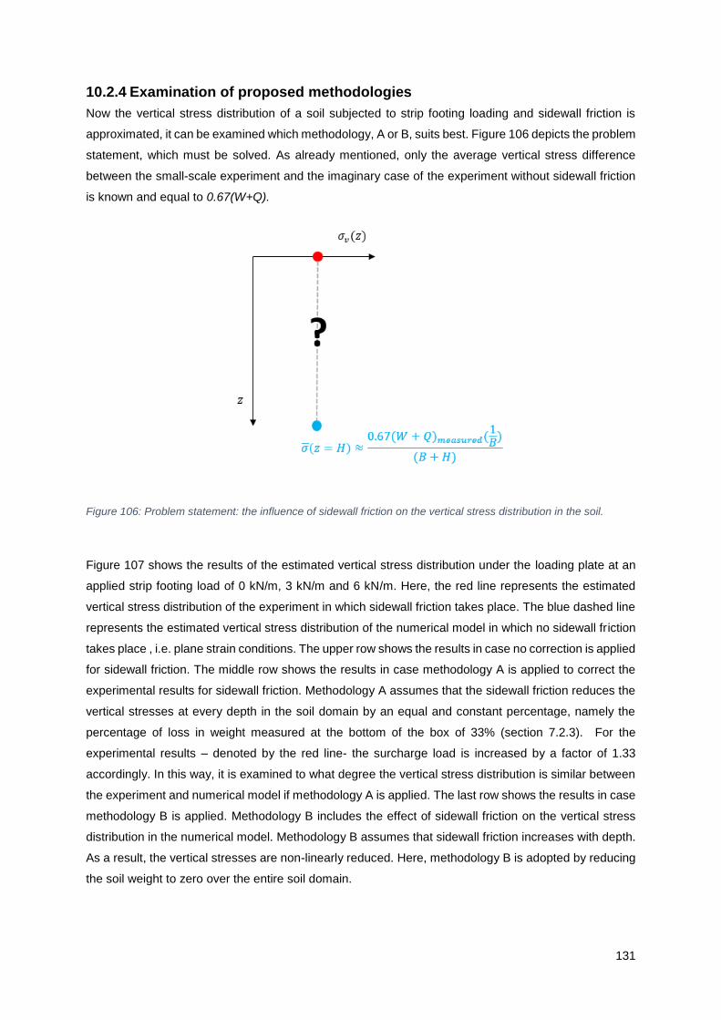
131
10.2.4 Examination of proposed methodologies
Now the vertical stress distribution of a soil subjected to strip footing loading and sidewall friction is
approximated, it can be examined which methodology, A or B, suits best. Figure 106 depicts the problem
statement, which must be solved. As already mentioned, only the average vertical stress difference
between the small-scale experiment and the imaginary case of the experiment without sidewall friction
is known and equal to 0.67(W+Q).
Figure 106: Problem statement: the influence of sidewall friction on the vertical stress distribution in the soil.
Figure 107 shows the results of the estimated vertical stress distribution under the loading plate at an
applied strip footing load of 0 kN/m, 3 kN/m and 6 kN/m. Here, the red line represents the estimated
vertical stress distribution of the experiment in which sidewall friction takes place. The blue dashed line
represents the estimated vertical stress distribution of the numerical model in which no sidewall friction
takes place , i.e. plane strain conditions. The upper row shows the results in case no correction is applied
for sidewall friction. The middle row shows the results in case methodology A is applied to correct the
experimental results for sidewall friction. Methodology A assumes that the sidewall friction reduces the
vertical stresses at every depth in the soil domain by an equal and constant percentage, namely the
percentage of loss in weight measured at the bottom of the box of 33% (section 7.2.3). For the
experimental results – denoted by the red line- the surcharge load is increased by a factor of 1.33
accordingly. In this way, it is examined to what degree the vertical stress distribution is similar between
the experiment and numerical model if methodology A is applied. The last row shows the results in case
methodology B is applied. Methodology B includes the effect of sidewall friction on the vertical stress
distribution in the numerical model. Methodology B assumes that sidewall friction increases with depth.
As a result, the vertical stresses are non-linearly reduced. Here, methodology B is adopted by reducing
the soil weight to zero over the entire soil domain.

132
The interface friction angle (𝛿) is taken 12.7° as derived from the Pull-up test in Chapter 7.2.2.
Considering the upper row of Figure 107 for which the results have not been corrected, the percentage
of the total weight transferred to the bottom of the box is 73% and 70% at 3 kN/m and 6 kN/m surcharge
load respectively. This percentage is close to the measured percentage of 67% of the total weight
transferred to the bottom of the box in Chapter 7.2.3. This observation increases the validity of the pull-
up test used to estimate the interface friction angle (𝛿) of 12.7° between the sand and sidewalls in the
small-scale experiment. In comparison, considering the interface friction angle of 4.8°, which was
determined with the Spring-suspension test, the percentage of the total weight transferred to the bottom
of the box is estimated to be 88.9% and 87.6% at 3 kN/m and 6 kN/m respectively.
Examining methodology A, the following can be observed:
• Reducing the surcharge load of the experimental results by 33% will result to a similar vertical
pressure in the soil at the bottom of the box, but will underestimate the vertical pressures at
lower depths. This underestimation will be highest at surface level.
Examining methodology B, the following can be observed:
• The lower figures show that the vertical pressures at every depth become close to the vertical
pressure distribution in the experiment in case of surcharge loads between 3 and 6 kN/m. The
difference in vertical pressure is reduced to less than 1.4 kPa.
• For loads >> 6 kN/m, the effect of the correction becomes negligible.
• or loads smaller than 3 kN/m, the soil weight induces a correction in the vertical stresses such
that the vertical stresses become smaller than the vertical stresses in the experiment at similar
surcharge load.

133
Figure 107: Estimated vertical stress distribution under the loading plate at an applied load of 0 kN/m, 3 kN/m and 6 kN/m. Here, the red line and blue dashed line represent the estimated vertical stress distribution of the experiment and numerical model respectively. The upper row shows the results in case no correction is applied for sidewall friction. The middle row shows the results in case methodology A is applied to correct the experimental results for sidewall friction. The last row shows the results in
case methodology B is applied to include the effect of sidewall friction on the vertical stress distribution in the numerical model.

134
10.2.5 Decision on methodology
Our main interest is the comparison of the soil-geogrid interaction and overall stability of the SPW
between the experimental and numerical model at ultimate limit state. Concludingly, methodology A will
not be a good correction as the soil pressures in the upper half of the soil domain will be significantly
underestimated. Methodology B results to acceptable small differences in the vertical stresses at all
depths for surcharge loads between 3-6 kN/m. Hence, the experimental and numerical models are
comparable for test configurations, whereby failure is reached at surcharge loads between 3-6 kN/m.
For experiments where failure is reached at surcharge loads < 3 kN/m, the stresses will be
underestimated if the soil weight is reduced to zero. Considering the experiments where failure is
reached for a surcharge load between 1-2.5 kN/m, the difference in vertical pressures will be minimized
by applying a reduction factor of 0.55 to the soil weight (see Figure 108).
Figure 108: Vertical stress distribution after applying a reduction factor of 0.55 to the unit soil weight. Figure a and b show the results at a surcharge load of 1 kN/m and 2.5 kN/m respectively.
Concludingly, the influence of sidewall friction is included in the numerical models according to
Methodology B by:
• Applying a reduction factor of 0 such that the soil weight is reduced to zero for the entire soil
domain for test configurations with a failure load ≥ 3 kN/m in the small-scale experiment.
• Applying a reduction factor of 0.55 such that the soil weight for the entire soil domain is reduced
by 45% for test configurations with a failure load < 3 kN/m geogrid in the small-scale experiment.

135
10.3 Comparison and evaluation of three different bottom boundary conditions
Assumptions have to be made, because the reality has to be modelled by a finite element method, which
connects the soil, sheet pile wall, footing, silicone block and test box boundaries by means of nodes
with a limited number of degrees of freedom to describe the true behaviour. Three different bottom
boundaries have been compared in order to find the bottom boundary conditions which fit best the
experimental results. In Figure 109, a close-up of the bottom boundary at the intersection of the soil,
SPW, silicone block and bottom of the test box. The yellow and pink elements represent the soil and the
silicone block respectively. The grey elements in Model 3 represents the bottom of the box. The blue
line represents the SPW. The white space between the dotted line and bottom boundary of the silicone
block represents the layer of air in Model 1 and Model 2. The red line connected at the bottom of the
blue line (SPW) in Model 1 represents the node-to-node anchor.
Figure 109: Close up of the connectivity plot visualizing the bottom boundary conditions.
For the bottom of Model 1 and Model 2, it was intended to create a bottom boundary such that the sheet
pile wall and silicone block can slide frictionless along the bottom. Both Model 1 and 2 realized
‘frictionless sliding’ by adding a 5 mm layer of air between the bottom boundary and the bottom of the
silicone block. Model 2 extends this layer of air such that as well the silicone block as the toe of the SPW
‘floats’ along the bottom. Vertical displacements are restricted such that the SPW and silicone block will
not ‘fall downward’. For both Model 1 and 2, the SPW is modelled 5 mm shorter and the silicone block
has no strength in the bottom 5 mm of its total height of 50 mm. The difference between Model 1 and
Model 2 is that Model 1 connects the toe of the SPW by a node-to-node anchor to the bottom boundary,
while Model 2 assigns a point displacement at the toe of the SPW, which allows the SPW to move freely
in horizontal direction and which constrains the SPW to move in vertical direction. Both models have
drawbacks. In Model 1, the sliding of the toe of the SPW is controlled by the stiffness chosen for the
node-to-node anchor. Therefore, a low stiffness (EA) of 5.5 MN is assigned to the node-to-node anchor
in order to minimize the resistance against sliding. In Model 2, the layer of air below the SPW results in

136
a gap between the sheet pile wall and bottom boundary through which displacement of the sand could
occur. Model 3 also includes the bottom of the test box. The SPW and silicone block are connected to
the bottom layer by means of an interface. Along the entire length of the bottom layer, free horizontal
displacement is prescribed while vertical displacement is not allowed. This way, a spurious failure
mechanism through the bottom layer is avoided. The first version of Model 3 did not implement a
prescribed displacement along the bottom of the test box was, but avoided a failure mechanism through
the bottom of the test box by making the bottom layer very stiff (E = 2.4·103 MPa). Because this model
was too sensitive to numerical instability, the prescribed displacement along the bottom of the box was
added in a second version of Model 3. The main difference between Model 3 and the other models is
therefore that some friction among the sheet pile wall, silicone block and soil has been included.
Based on the failure mechanism, sheet pile wall deformation and soil displacement-load curves the
model which best corresponds to the experimental results is chosen. The experimental results of Test
22, which includes a two-layer-geogrid anchorage, is taken as a validation test. Methodology B is applied
to all three models such that the unit soil weight is zero.
10.3.1 Failure mechanism
Figure 110 shows the output results of PLAXIS from the total soil displacements for Model 1, Model 2
and Model 3 at a load level of ~4 kN/m. The legends deviate between the colour plots for clarity reasons:
the figure is only meant to provide an insight into the soil displacements fields within each model. Dark
blue means zero displacements, while a dark red colour indicates relatively high soil displacements.
Accordingly, soil displacements increase from dark blue-light blue-yellow-orange to dark red. The light
blue soil displacements at surface level behind the loading plate are the result of numerical errors. These
arise from the high gradients at the outer edge of the load plate.
Figure 110: Total soil displacements for model 1, model 2 and model 3 at a load level of ~4 kN/m.
Models 1 and 2 show a similar development of displacement fields in the soil, both on the active and
passive side. The main difference which can be observed between Model 1-2 and Model 3, is that the
soil displacements in the silicone block and just behind the SPW show a more translational mode of
failure in case of Model 1-2 and a combination of a translational and rotational mode of failure in case
of Model 3.

137
10.3.2 Relation between soil displacements and applied load
Figure 102 shows the total soil displacements as a function of the applied load for Model 1, Model 2 and
Model 3, which are corrected for sidewall friction. The results of the numerical model are compared with
the experimental results obtained from GeoPIV-RG and the manually tracking. The soil displacements
are given for a point in the soil domain indicated by the red square in the schematization of the test set-
up, which is depicted in the bottom right corner.
Figure 111: Total soil displacements as a function of the applied load for Model 1, Model 2 and Model 3, which are corrected for sidewall friction. The soil displacements are given for a point in the soil domain indicated by the red square in the schematization of the test set-up, which is depicted in the
bottom right corner.

138
From the soil displacement-load curves, it can be observed that the soil displacement is significantly
overestimated by Model 1 and Model 2, while Model 3 shows good similarity at applied loads > 3.5
kN/m. Apparently, the combination of translational and rotational mode of failure as described in Section
10.3.1 is more true to the mechanisms occurring in the experiment. Some kind of internal shear
behaviour in the silicone block affects the mobilised passive resistance. The latter agrees with our
observations during testing. We had observed that the silicone block was compressed by the SPW non-
uniformly along its height. The deformation in the silicone block cannot be measured by means of DPIV
as the texture of the silicone block is too low.
10.3.3 Sheet pile wall deformation
Figure 112 shows the SPW displacement for the numerical models and the experimental results. Since
the automatically tracking of the SPW from the photos of the test is not always very accurate, it was
decided to manually track several points along the height of the SPW. Accordingly, some apparent
bending of the SPW seems to occur. This is the consequence of inaccuracies in the manual tracking.
Figure 112: SPW deformation at an applied load of 3.7 kN/m for the experiment and numerical models corrected for sidewall friction.
From the results, it can be concluded that including a frictional bottom boundary yields better agreement
with the experimental results. Accordingly, it is decided to model the bottom boundary conditions
according to Model 3.

139
11 Numerical results and analysis
This chapter gives the results of the 2D numerical model of the following small-scale test configurations:
• one 18 cm geogrid-anchor and the load positioned 13 cm from the SPW,
• one 18 cm geogrid-anchor and the load positioned 3 cm from the SPW,
• two geogrid-anchors (18 cm top geogrid and 11 cm bottom geogrid) and the load positioned
3 cm from the SPW.
Section 11.1 analyses the failure mechanism and Section 11.2 looks at the development of tensile force
distribution along the geogrid in order to investigate:
1. the influence of the load position on the tensile force distribution and
2. the influence of the bottom geogrid-anchor on the top geogrid-anchor.
The models have been corrected for sidewall friction, which means that the soil weight has been reduced
to zero22. In reality, some shear stress will be mobilised due to the weight of the soil. However, the shear
stress mobilised due to the weight of the soil is relatively small compared to the shear stress mobilised
due to the surcharge load. Hence, a more or less similar distribution of frictional forces along the
geogrid(s) would be expected if the soil weight had been included in the numerical model.
11.1 Global failure mechanism
11.1.1 Influence of the load position
In order to investigate the influence of the load position on the tensile force distribution in the geogrid,
we first look at the global failure mechanisms for:
• a load plate positioned partly behind the geogrid-anchor, i.e. the distance of the outer edge of
the loading plate from the SPW > length of the geogrid-anchor. The model includes an 18 cm
geogrid-anchor and the load is positioned 13 cm to 23 cm from the SPW.
• a loading plate positioned above the geogrid-anchor, i.e. the distance of the outer edge of the
loading plate from the SPW < length of the geogrid-anchor. The model includes an 18 cm
geogrid-anchor and the loading plate is positioned 3 to 13 cm from the SPW.
22 All three tests that were analysed in this chapter failed at a load ≥ 3 kN/m. Therefore, a reduction factor of zero is applied to
the soil weight.
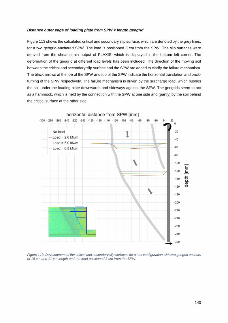
140
Distance outer edge of loading plate from SPW < length geogrid
Figure 113 shows the calculated critical and secondary slip surface, which are denoted by the grey lines,
for a two geogrid-anchored SPW. The load is positioned 3 cm from the SPW. The slip surfaces were
derived from the shear strain output of PLAXIS, which is displayed in the bottom left corner. The
deformation of the geogrid at different load levels has been included. The direction of the moving soil
between the critical and secondary slip surface and the SPW are added to clarify the failure mechanism.
The black arrows at the toe of the SPW and top of the SPW indicate the horizontal translation and back-
turning of the SPW respectively. The failure mechanism is driven by the surcharge load, which pushes
the soil under the loading plate downwards and sideways against the SPW. The geogrids seem to act
as a hammock, which is held by the connection with the SPW at one side and (partly) by the soil behind
the critical surface at the other side.
Figure 113: Development of the critical and secondary slip surfaces for a test configuration with two geogrid anchors of 18 cm and 11 cm length and the load positioned 3 cm from the SPW.

141
Distance outer edge of loading plate from SPW > length geogrid
Figure 103 shows the critical and secondary slip surface, which are denoted by the grey lines, for a
single-anchored SPW and the load positioned 13 cm from the SPW. The length of the anchor is 18 cm.
The slip surfaces were derived from the shear strain output of PLAXIS, which is displayed in the left
corner. It shows that the critical slip surface now goes from the outer edge of the footing plate at ground
surface level to the toe of the SPW. The secondary slip surface has not fully developed yet. The
deformation of the geogrid at different load levels has been included. The rear part of the geogrid is
pushed downward by the soil in the active zone. Here, the geogrid is hold in place by the connection
with the SPW only. The black arrows at the toe and top of the SPW indicate the horizontal translation
and overturning of the SPW respectively. The failure mechanism is again driven by the surcharge load.
Figure 114: Development of the critical and secondary slip surfaces for a test configuration with an 18 cm geogrid and the load positioned 13 to 23 cm from the SPW.

142
11.1.2 Influence of the number of geogrids
In Chapter 9, it was observed that the critical slip surface for the double geogrid-anchorage was slightly
more curved at the height of the bottom geogrid-anchor compared to the single geogrid-anchored SPW.
This section compares the numerical models with one and two geogrids. We will successively compare
the following: the total soil displacements at a similar load level, the slip surfaces, and the axial force in
the SPW at similar load level. This way, it is investigated whether the two-geogrid configuration transfers
more force to the SPW than the one grid configuration.
Figure 115 shows the PLAXIS output of the total soil displacements for (a) the model with an 18 cm
geogrid-anchor and (b) the model with two geogrid-anchors (18 cm top geogrid-anchor and 11 cm
bottom geogrid-anchor). The soil displacements are compared at a load level of ~5 kN/m. The total soil
displacement ranges between 0 (dark blue) and 12 (red) mm. The high displacements at ground surface
level left of the loading plate are produced by unstable computation results, which are due to the high
stiffness gradients in the corner of the loading plate. These local peak values should be neglected for
our analysis. The main observation from this figure are the significantly higher soil displacements in
case of a single-anchored SPW. We observe an increase of approximately 30% in the total soil
displacements in the active zone.
Figure 115: Total soil displacement at a load level of ~5 kN/m for an SPW anchored by (a) one 18 cm geogrid and (b) one top
18 cm geogrid and bottom 11 cm geogrid.

143
Figure 116 shows the critical and secondary slip surface of the double geogrid-anchored SPW and the
single anchored SPW for a load positioned 3 cm from the SPW. The locations of both geogrids are
denoted by the dashed grey lines. The critical slip surface initiates at the outer edge of the loading plate
and the secondary slip surface at the inner edge of the loading plate. The critical slip surface and the
secondary slip surface intersect the SPW with an angle of 31° and 16° to the vertical respectively. It can
be observed that the critical slip surface circumvents the bottom geogrid. As a result, a slightly more
curved and wider critical slip surface has developed in the two-geogrids configuration.
Figure 116: Critical and secondary slip surfaces for geogrid-anchorage of two geogrids (18 cm top geogrid and 11 cm bottom geogrid) or just one top 18 cm geogrid-anchor. The dashed black lines are the critical and secondary slip surface of the test with one 18 cm geogrid-anchor. The continuous black lines are the critical and secondary
slip surface of the test with two geogrid-anchors.

144
Figure 117 shows the axial force in the SPW for the model with a double geogrid-anchorage and the
model with a single geogrid-anchorage. For the double anchored SPW, a sharp increase in axial force
at the depth of the anchor point of the second geogrid is observed. At the toe of the modelled SPW, a
maximum difference of 0.16 kN/m, i.e. an increase of 10%, is found.
Figure 117: Axial force in SPW for a double geogrid-anchored SPW and a single geogrid-anchored SPW at an
applied surcharge load of 5 kN/m. Compressive forces have a negative sign.
11.2 Tensile force distribution along the geogrid anchorage
Our main interest is the investigation of the tensile force distribution along the geogrid-anchorage. This
is the most direct way to study the resistance that can be provided by a geogrid-anchor. Due to the soil
shear stresses along the top and bottom of the geogrid, a tensile force can develop in the geogrid, which
is the force – provided by the geogrid-anchor - resisting the SPW from failing. Finally, this is the force
which must be – at least – equal to the required anchor force calculated for the design of the SPW. The
advantage of the numerical model is that the stresses in the soil and structures can be inspected, in
contrary to the experiments conducted. Both the frictional forces along the geogrid as well as the tensile
force in the geogrid are analysed. First, the development of the tensile force distribution under an
increasing surcharge load for the following two models is analysed:
• Model consisting of a double geogrid-anchored SPW and the load positioned above the
geogrids, i.e. 3 cm from the SPW. The top geogrid and bottom geogrid have a length of 18 cm
and 11 cm respectively.
• Model consisting of a single geogrid-anchored SPW and the load positioned partly behind the
geogrid, i.e. 13 cm from the SPW. The geogrid has a length of 18 cm.

145
Beside the tensile force distribution, we will look at the deformation of the geogrid-anchor in the soil at
different load levels in order to link the development of both the tensile force and the deformation.
Second, the influence of the load position on the tensile force distribution along the geogrid is analysed.
Third, the influence of the bottom geogrid on the top geogrid is analysed.
11.2.1 Development of tensile force distribution in two-geogrids anchorage
Figure 118 shows the deformation of the top 18 cm geogrid-anchor at different load levels. The loading
plate is positioned 3 to 13 cm distance from the SPW. It can be observed that the part of the geogrid
below the footing deforms mainly vertically downward. The deformation looks a bit like a hammock. The
deformed geogrid follows the non-homogenous settlement of the loading plate. The loading plate settles
more on the outer part (with respect to the SPW) due to the sliding soil mass along the critical slip
surface. A more or less equal magnitude of vertical displacement is observed from a load level of 0 kN/m
to 5.0 kN/m as between a load level from 5.0 kN/m to 6.8 kN/m. From a load level of 5.0 kN/m, pull-out
of the geogrid can be observed very clearly. Hence, signs of failure are present.
Figure 118: Deformed top geogrid-anchor at different load levels (two-geogrid configuration).
Figure 119 shows the tensile force distribution along the 18 cm top geogrid-anchor for different load
levels. A maximum anchor force of 1.6 kN/m is reached at a load level of 5.7 kN/m. The grey lines, which
are numbered A to E separate the curves in zones of very roughly constant tensile force gradients. Since
the gradient of the tensile force is an indication of the amount of friction developed in the soil-geogrid
interface, these zones can be considered as different strain fields. The zones were drawn for the tensile
force distribution at a load level of 5.7 kN/m. Line C and D could be neglected for load levels ≤ 5.0 kN/m.
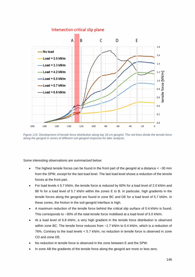
146
Figure 119: Development of tensile force distribution along top 18 cm geogrid. The red lines divide the tensile force along the geogrid in zones of different soil-geogrid response for later analysis.
Some interesting observations are summarized below:
• The highest tensile forces can be found in the front part of the geogrid at a distance < ~30 mm
from the SPW, except for the last load level. The last load level shows a reduction of the tensile
forces at the front part.
• For load levels ≤ 5.7 kN/m, the tensile force is reduced by 60% for a load level of 2.0 kN/m and
88 % for a load level of 5.7 kN/m within the zones E to B. In particular, high gradients in the
tensile forces along the geogrid are found in zone BC and DE for a load level of 5.7 kN/m. In
these zones, the friction in the soil-geogrid interface is high.
• A maximum reduction of the tensile force behind the critical slip surface of 0.4 kN/m is found.
This corresponds to ~30% of the total tensile force mobilised at a load level of 5.0 kN/m.
• At a load level of 6.8 kN/m, a very high gradient in the tensile force distribution is observed
within zone BC. The tensile force reduces from ~1.7 kN/m to 0.4 kN/m, which is a reduction of
76%. Contrary to the load levels < 5.7 kN/m, no reduction in tensile force is observed in zone
CD and zone DE.
• No reduction in tensile force is observed in the zone between E and the SPW.
• In zone AB the gradients of the tensile force along the geogrid are more or less zero.
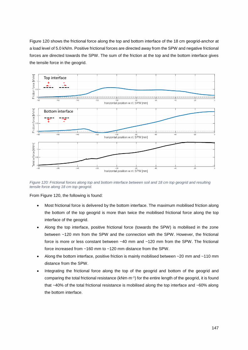
147
Figure 120 shows the frictional force along the top and bottom interface of the 18 cm geogrid-anchor at
a load level of 5.0 kN/m. Positive frictional forces are directed away from the SPW and negative frictional
forces are directed towards the SPW. The sum of the friction at the top and the bottom interface gives
the tensile force in the geogrid.
Figure 120: Frictional forces along top and bottom interface between soil and 18 cm top geogrid and resulting tensile force along 18 cm top geogrid.
From Figure 120, the following is found:
• Most frictional force is delivered by the bottom interface. The maximum mobilised friction along
the bottom of the top geogrid is more than twice the mobilised frictional force along the top
interface of the geogrid.
• Along the top interface, positive frictional force (towards the SPW) is mobilised in the zone
between ~120 mm from the SPW and the connection with the SPW. However, the frictional
force is more or less constant between ~40 mm and ~120 mm from the SPW. The frictional
force increased from ~160 mm to ~120 mm distance from the SPW.
• Along the bottom interface, positive friction is mainly mobilised between ~20 mm and ~110 mm
distance from the SPW.
• Integrating the frictional force along the top of the geogrid and bottom of the geogrid and
comparing the total frictional resistance (kNm·m-1) for the entire length of the geogrid, it is found
that ~40% of the total frictional resistance is mobilised along the top interface and ~60% along
the bottom interface.

148
Figure 121 shows the deformed bottom geogrid-anchor of 11 cm at different load levels. Compared to
the deformation of the top geogrid-anchor, a sharper deformation is observed at the front part. The
hammock shape of the 18 cm geogrid-anchor has been altered as the 11 cm geogrid-anchor has almost
no length outside the critical slip surface. For the 11 cm geogrid-anchor it can be observed that the rear
end is entirely dragged along within the active zone, except for the last loading step of 6.8 kN/m.
Figure 121: Deformed bottom geogrid-anchor at different load levels. The load is positioned 3 cm from the SPW. Accordingly, the inner edge and outer edge of the loading plate are located 30 mm and 130 mm from the SPW.
Figure 122 shows the tensile force distribution of the bottom geogrid-anchor of 11 cm. The intersection
of the geogrid with the critical slip surface is indicated.
Figure 122: Development of tensile force distribution along bottom 11 cm geogrid-anchor for a double geogrid-anchored SPW.

149
From Figure 122 and Figure 123, the following has been found for the bottom geogrid:
• At a load level of 6.8 kN/m, the tensile force has reduced at the front part of the SPW.
• Comparing the lower load levels with the higher load level, a shift in the distribution of the tensile
force can be observed. For load levels ≤ 3.3 kN/m, highest tensile force is observed close to the
SPW. For load levels > 3.3 kN/m, the maximum tensile force is located at ~60 mm from the
SPW.
• For load levels ≤ 2.0 kN/m, tensile forces reduce from the connection with the SPW to zero at
the rear end of the geogrid. The gradient is relatively small.
• For load levels ≥ 3.3 kN/m, tensile forces reduce from a maximum value at 60 mm from the
SPW to zero at the rear end. Hence, a steeper gradient is observed compared to gradients of
the tensile force at lower load levels.
Figure 123 shows the frictional force along the top and bottom interface of the 18 cm geogrid-anchor at
a load level of 5.0 kN/m. Positive frictional forces are directed away from the SPW and negative frictional
forces are directed towards the SPW. The sum of the friction at the top and the bottom interface gives
the tensile force in the geogrid.
From Figure 123, the following is found:
• Almost all positive friction is mobilised along the bottom interface within the first 100 mm from
the SPW.
• The tensile force is reduced by 50% due to the negative friction along the top interface within
the first 60 mm from the SPW.
Figure 123: Frictional forces along top and bottom interface between soil and 11 cm bottom geogrid and resulting tensile force along 11 cm bottom geogrid.

150
11.2.2 Development of tensile force distribution for load positioned partly behind geogrid-anchor
This chapter looks at the load positioned 13 cm to 23 cm from the SPW. Figure 124 shows the
deformation of the 18 cm geogrid-anchor at different load levels. The end part of the geogrid is pushed
downwards. Although the SPW displacements were not very large (~5 mm), no stable solution could be
computed (stiffness parameter CSP < 0.015) for an applied load > 3.0 kN/m. So, the soil failed in the
numerical calculation (Plaxis bv., 2019)
Figure 124: Deformed 18 cm geogrid-anchor at different load levels. The loading plate is positioned 13 cm to 23 cm from the SPW.
Figure 125 shows the tensile force distribution along the 18 cm geogrid-anchor at different load levels.
The red line indicates the location of the intersection between the geogrid and the critical slip surface.
Figure 125: Tensile force distribution along 18 cm geogrid-anchor at different load levels. The loading plate is
positioned 13 cm to 23 cm from the SPW.

151
Figure 126 gives the frictional forces along the top and bottom interface of the geogrid and the resulting
tensile force distribution for the surcharge load of 3.0 kN/m. Positive frictional forces are directed away
from the SPW and negative frictional forces are directed towards the SPW.
Figure 126: Frictional force along top and bottom interface and tensile force along 18 cm geogrid at an applied load
of 3.0 kN/m. The loading plate is positioned 13 cm to 23 cm from the SPW.
The following is observed from Figure 125 and Figure 126:
• The maximum tensile forces increase with increasing load level.
• The tensile forces remain more or less constant from the connection with the SPW to ~140 mm
distance from the SPW. Tensile forces reduce between ~140 mm distance from the SPW and
the rear end of the geogrid.
• Nonzero tensile forces are observed at the rear end of the geogrid for load levels ≥ 2.0 kN/m.
• Almost all positive friction is mobilised along the bottom interface at a distance > 120 mm from
the SPW.
• Negative friction is mobilised between ~80 mm and ~140 mm from the SPW.
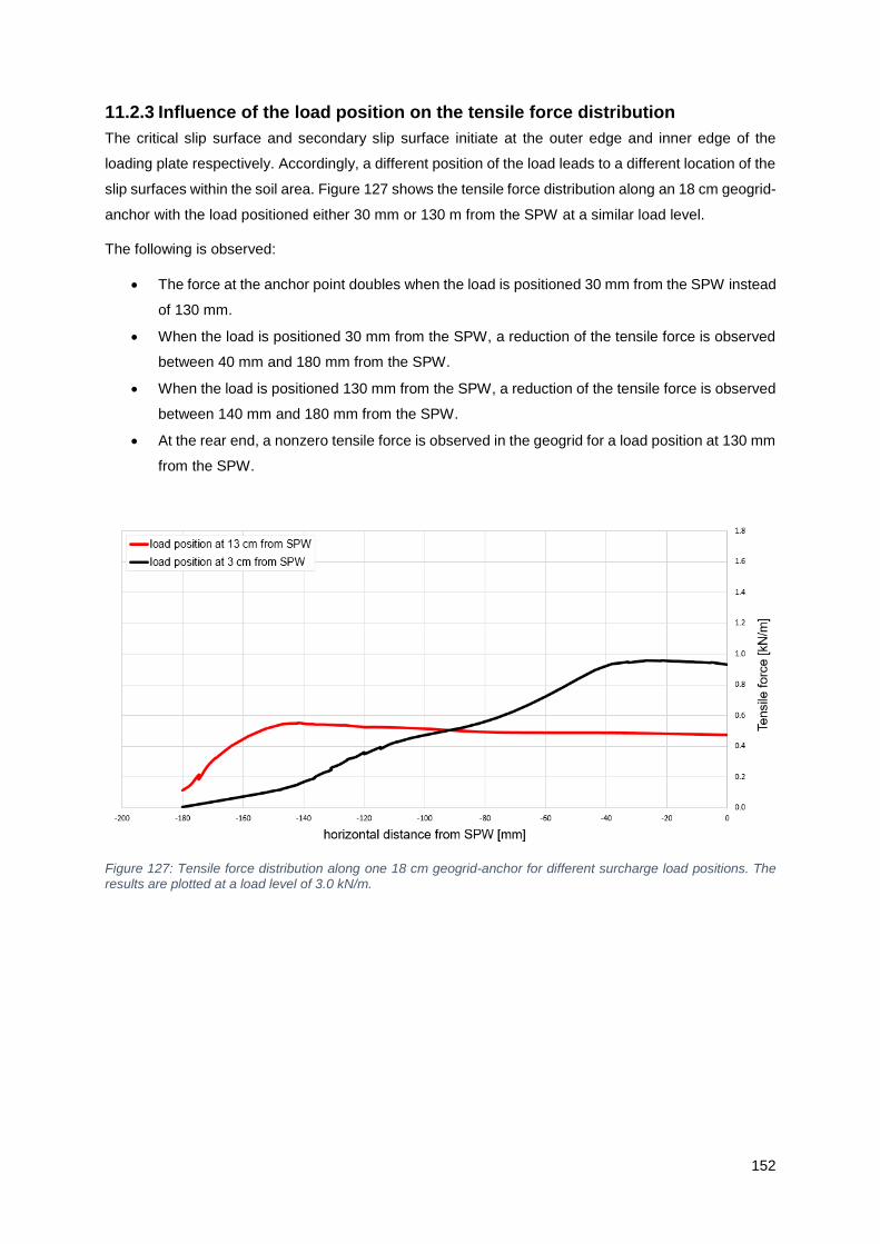
152
11.2.3 Influence of the load position on the tensile force distribution
The critical slip surface and secondary slip surface initiate at the outer edge and inner edge of the
loading plate respectively. Accordingly, a different position of the load leads to a different location of the
slip surfaces within the soil area. Figure 127 shows the tensile force distribution along an 18 cm geogrid-
anchor with the load positioned either 30 mm or 130 m from the SPW at a similar load level.
The following is observed:
• The force at the anchor point doubles when the load is positioned 30 mm from the SPW instead
of 130 mm.
• When the load is positioned 30 mm from the SPW, a reduction of the tensile force is observed
between 40 mm and 180 mm from the SPW.
• When the load is positioned 130 mm from the SPW, a reduction of the tensile force is observed
between 140 mm and 180 mm from the SPW.
• At the rear end, a nonzero tensile force is observed in the geogrid for a load position at 130 mm
from the SPW.
Figure 127: Tensile force distribution along one 18 cm geogrid-anchor for different surcharge load positions. The results are plotted at a load level of 3.0 kN/m.

153
11.2.4 Influence of the bottom geogrid-anchor on the top geogrid-anchor
Both geogrid-anchors must mobilise tensile force obtained from interaction mechanisms with the
surrounding soil. The soil can only be mobilised ones. When the soil has already been mobilised by the
interaction with the bottom geogrid, this may reduce the mobilised tensile forces in the top geogrid. The
influence of the bottom geogrid on the top geogrid is investigated by comparing the single geogrid-
anchorage system with the double geogrid-anchorage systems, whereby both anchorage systems
contain a top 18 cm geogrid.
Figure 128 shows the deformed top 18 cm geogrid for the double geogrid-anchorage and the single
geogrid-anchor at two load levels. The dashed lines and continuous lines correspond to the single
geogrid-anchorage and double geogrid-anchorage respectively.
The main findings are:
• The single geogrid-anchorage is vertically displaced more than the double geogrid-anchorage.
• The more the geogrid is displaced vertically, the longer the ‘vertical’ parts of the geogrid along
the critical and secondary slip surface located around 130 mm and 30 mm from the SPW.
• Due to the larger displacements downward, the part of the geogrid located in the critical slip
surface has moved slightly closer to the SPW.
Figure 128: The deformed top geogrid of 18 cm at two load levels.

154
In Figure 129, the tensile force distribution along the top 18 cm geogrid for the single and double geogrid-
anchorage are compared at a load level of 3.8 kN/m and ~5.0 kN/m. Again, the single geogrid-anchorage
and double geogrid-anchorage are given by a dashed and continuous line respectively. The colour of
the curves denotes the load level. By means of two grey lines, the zone is indicated where deviation is
observed between the results of the single geogrid-anchorage and double geogrid-anchorage.
Between ~115 mm and ~130 mm distance from the SPW, the tensile force in the 18 cm top geogrid of
the double geogrid-anchorage remains more or less constant, while the tensile force reduced along the
18 cm top geogrid for the single geogrid-anchorage. At 160 mm distance from the SPW, the curves
coincide.
Figure 129: Tensile force distribution along top 18 cm geogrid at two load levels for one and two-geogrid anchorage system at a load of ~ 5 kN/m (the load level was 4.8 kN/m and 5.0 kN/m for the single geogrid-anchorage system
and the double-anchorage system respectively.
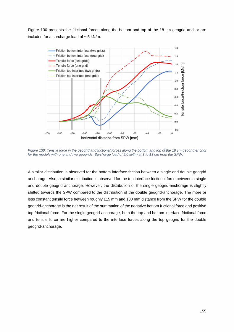
155
Figure 130 presents the frictional forces along the bottom and top of the 18 cm geogrid anchor are
included for a surcharge load of ~ 5 kN/m.
Figure 130: Tensile force in the geogrid and frictional forces along the bottom and top of the 18 cm geogrid-anchor for the models with one and two geogrids. Surcharge load of 5.0 kN/m at 3 to 13 cm from the SPW.
A similar distribution is observed for the bottom interface friction between a single and double geogrid
anchorage. Also, a similar distribution is observed for the top interface frictional force between a single
and double geogrid anchorage. However, the distribution of the single geogrid-anchorage is slightly
shifted towards the SPW compared to the distribution of the double geogrid-anchorage. The more or
less constant tensile force between roughly 115 mm and 130 mm distance from the SPW for the double
geogrid-anchorage is the net result of the summation of the negative bottom frictional force and positive
top frictional force. For the single geogrid-anchorage, both the top and bottom interface frictional force
and tensile force are higher compared to the interface forces along the top geogrid for the double
geogrid-anchorage.

156
11.3 Analysis of results
11.3.1 Global failure mechanism
Influence of load position
In agreement with the experimental results, it has been observed that the load position influences the
developed slip surfaces. The critical and secondary slip surfaces initiate at the outer edge and inner
edge of the loading plate respectively. Accordingly, the active zone is also for the numerical model
enclosed by the critical and secondary slip surface. Similar to the experimental results, a curved critical
slip plane is observed with an intersection normal to the initially horizontal positioned geogrid as shown
in Figure 116. The geogrid in the active zone is dragged downward with the soil. The geogrid deforms
like a hammock due to the connection with the SPW on one side and resistance from the soil outside
the critical slip surface on the other side. When the geogrid only intersects the secondary slip surface,
the geogrid deformations is characterized by a downward displacing rear end, while the geogrid is hold
in place by the connection with the SPW.
Influence of number of geogrids
In agreement with the experimental results, it has been observed that, if a second geogrid anchors is
applied, the bottom geogrid-anchor alters the critical slip surface. Compared to the critical slip surface
for a single 18 cm top geogrid-anchorage, a wider critical slip surface is observed for the double geogrid-
anchored SPW. The critical slip surface circumvents the bottom geogrid-anchor.
11.3.2 Tensile force along the geogrid anchorage
For the analysis we separate the soil in three zones, according to the zones defined in Chapter 7 and
depicted in Figure 99.
First, the general findings regarding the tensile force distribution along the geogrid-anchor are described
for:
• a double geogrid-anchored SPW with the load positioned above the geogrid.
• an 18 cm geogrid-anchored SPW with the load positioned partly behind the geogrid-anchor.
Second, the tensile force distribution is analysed with regard to the (1) influence of the load position and
(2) the influence of the bottom geogrid on the mobilised tensile force in the top geogrid.

157
Mobilised tensile force along the top geogrid for a distance between the outer edge of the
loading plate and the SPW < geogrid length
Top geogrid
Linking the observed critical and secondary slip surfaces from Figure 113 to the tensile force distribution
along the top geogrid, the following can be concluded:
• No shear resistance is provided by the soil enclosed by the SPW and the secondary slip surface
(zone I according to Figure 99).
• Tensile force is transferred to the soil in the active zone (zone II according to Figure 99).
• When the load level increases, relatively more tensile force is transferred to the soil in zone II
compared to zone III.
• The maximum mobilised friction along the bottom of the top geogrid is more than twice the
maximum mobilised frictional force along the top interface of the top geogrid.
• The friction along the bottom interface is mobilised along the part of the geogrid below the
loading plate as depicted in Figure 131.
• The friction along the top interface is mobilised along the ‘inclined’ parts of the geogrid as
depicted in Figure 131.
Figure 131: Most important mobilised frictional forces along the top and bottom interface of the top 18 cm geogrid-anchor. The green arrows indicate the positive friction and the red arrows the negative friction.

158
Bottom geogrid
Linking the observed critical and secondary slip surfaces (Figure 113) to the tensile force and frictional
force distribution (Figure 122 - Figure 123) and the deformation of the bottom geogrid (Figure 121), the
following can be concluded for the bottom geogrid-anchor:
• Almost all tensile force is mobilised due to the shear resistance along the bottom interface.
• No contribution to the resistance was provided by the interaction of the geogrid with the soil
above the bottom geogrid. The shearing soil along the top geogrid even caused a reduction of
the tensile force, which is represented by a negative frictional force in Figure 122.
• The frictional forces mobilised along the bottom geogrid-anchor are visualised in Figure 132.
The distribution of the bottom friction is similar to the one of the top geogrid-anchor. The only
difference is the negative friction, which is mobilised between 10 mm and 60 mm from the SPW.
A clarification may be given by the failure points computed by PLAXIS. The output is included
in Figure 132. The slip surface which has developed between the secondary and critical slip
surface may cause the negative frictional forces along the top interface.
Figure 132: Most important mobilised friction along the top and bottom interface of the 11 cm bottom geogrid-
anchor. The green arrows indicate the positive friction and the red arrows the negative friction.

159
Analysis
From the analysis of the mobilised frictional forces in Figure 131 and Figure 132, the following is
hypothesized:
• The positive friction along the top interface is mobilised due to the relative displacement
between soil-geogrid, which is caused by the sliding soil mass in the active zone. Due to the
sliding soil mass, the geogrid is pulled out of the soil behind the critical slip surface. Accordingly,
we believe that the part of the geogrid outside the active zone makes the mobilisation of positive
frictional forces along the top geogrid possible.
• The positive friction along the bottom interface in the active zone does not depend on the part
of the geogrid behind the active zone. However, the connection with the SPW is necessary for
the mobilisation of friction along the bottom of the geogrid. Due to the connection at the anchor
point, the geogrid acts as a kind of barrier net which resists the movement of the soil downward
and towards the SPW. Due to the relative displacement between the rough geogrid-soil
interface, frictional forces can be mobilised.
• It is believed that the development of the shallow slip surface at larger load levels can be
prevented from developing when the spacing between the geogrids is smaller. The shallow slip
surface initiates at the outer edge and travels between the top and bottom geogrid towards the
SPW. If the vertical spacing between the top and bottom geogrid is too large, negative frictional
forces must be taken into account along the top interface of the bottom geogrid-anchor for the
computation of the mobilised tensile forces.
Figure 133 visualises the basic ideas obtained from our analysis. The tensile force in the top and bottom
geogrid are mobilised due to frictional forces along the top of both geogrids behind the critical slip surface
(zone III) and frictional forces along the bottom of both geogrids in the active zone (zone II). The curved
shape of the slip surfaces is assumed to be curved due to the interaction with the geogrids, which
mobilises shear stresses at the intersection. This relation is also found in Figure 116 for the numerical
models and Figure 80 for the experiments. According to minimum energy principles, it can be assumed
that the initial slip surfaces are straight. In the experiments, straight slip surfaces were also observed
for test configurations with short geogrid-anchors, which did not intersect with the critical slip surface.
Accordingly, straight slip surfaces are considered for the division of the three zones.

160
Figure 133: Schematization of the basic idea behind the developed frictional forces in the geogrid-anchorage.
Figure 134 shows the tensile forces and frictional forces in and along the top geogrid of the numerical
model, which simulates one of the geogrid-anchored SPWs for the construction of Windpark Krammer
on prototype scale (van Duijnen et al., 2021). Anchor 3 is the top anchor of three anchors, and has been
wrapped around a horizontal steel pipe. The steel pipe was attached to the SPW. As a consequence,
the anchor consists of two layers of geogrid. The bottom layer and top layer are denoted by the number
3.1 and 3.2 respectively. In Figure 120, positive frictional force indicates a force pointing in the direction
away from the SPW, while a negative frictional force indicates a force pointing towards the SPW. The
sum of the forces will give the tensile force. Figure 134 uses an alternative sign convention. Here, the
positive and negative sign are related to the direction relative to the geogrid. Accordingly, a positive
frictional force will act towards the SPW for top interfaces and away from the SPW for bottom interfaces.
The first ~ 3.8 m behind the SPW correspond with the part which has been modelled in the small-scale
experiment by the 18 cm geogrid anchor. This front part is denoted by the white background in Figure
134.

161
Figure 134: Calculated tensile force in the geogrid and frictional force in the interfaces along the two geogrids of anchor 3 of one of the geogrid-anchored SPWs for the construction of the Windpark Krammer (van Duijnen et al.,
2021).
Figure 135: Geogrid-anchored SPW at Windpark Krammer as presented by van Duijnen et al. (2021). They designed the length of the geogrids from the bottom to the top, assuming the effective anchorage length (green segments in the figure) starting from the rear end of the underlying anchor. This picture has been mirrored in comparison to Figure 134.

162
By comparing our results (Figure 130) with the numerical results of van Duijnen et al. (2021) in Figure
134 on prototype scale for the front part of the geogrid-anchorage (white background), the following
(dis)similarities are found:
• In both models friction is mobilised within the active zone.
• In the numerical model of the prototype, the frictional force provided by the top interface of the
top geogrid is ~30% lower than the frictional force provided by the bottom interface of the bottom
geogrid at the anchor point. In the numerical model of the small-scale experiment, the frictional
force provided by the top interface is 88% lower than the frictional force provided by the bottom
interface at the anchor point.
• For the part of the geogrid under consideration (the front part) of the numerical model of the
prototype, the highest share, around 60%, of the total resistance is provided by the top interface
of the top geogrid and around 40% is provided by the bottom interface of the bottom geogrid. In
the numerical model of the small-scale experiment, approximately 45% of the total resistance
is provided by the top interface and 55% of the total resistance is provided by the bottom
interface.
• Both numerical models show that a significant portion of the friction along the bottom interface
of the (bottom) geogrid is mobilised in the active zone. In the numerical model of the prototype,
an increase in frictional force of approximately a factor 5 is observed from the critical slip surface
to the connection with the SPW. In the numerical model of the small-scale experiment, the
frictional force has increased by a factor of ~ 13 from the critical slip surface to the connection
with the SPW.
• Both numerical models show that shear stresses along the top of the (top) geogrid reduce the
frictional force close to the SPW and increase the frictional force along the (top) of the geogrid
behind the active zone.
Concludingly, similar soil-geogrid interaction has been observed between both numerical
models except that a relatively higher share of resistance is provided by the friction along the
top of the geogrid-anchor in the numerical model of the prototype.

163
Mobilised tensile force along geogrid for a distance between the outer edge of the loading plate
and the SPW > geogrid length
Linking the observed critical and secondary slip surfaces (Figure 114), the tensile force and frictional
force distribution along the bottom geogrid-anchor (Figure 125 and Figure 126) and the deformation of
the 18 cm geogrid (Figure 124), the following can be concluded:
• The soil in ‘zone I’ does not provide any shear resistance along the geogrid-anchor. Since the
soil is weightless in the model and the load is not transferred to the soil at a distance < ~100 mm
from the SPW, no shear can be mobilised.
• The friction along the bottom interface between soil and geogrid almost entirely defines the
mobilised tensile force in the geogrid.
• The friction along the bottom interface is mobilised in the active zone, zone II. From the
intersection with the secondary slip surface at ~100 mm distance from the SPW until the
connection with the SPW, no additional friction is mobilised.
Accordingly, the distribution of the frictional forces looks similar to the front part of the distribution of
Figure 131. Part of the resistance is missing as the geogrid intersects only the secondary slip surface.
Figure 136: Most important mobilised friction along the top and bottom interface of the 18 cm geogrid-anchor. The load is positioned 13 cm to 23 cm from the SPW. The green arrows indicate the positive friction and the red arrows the negative friction.

164
Influence of load position on tensile force distribution
From Figure 127, it can be concluded that:
• The mobilised tensile force depends on the load position, because the load position defines the
critical and secondary slip surface and accordingly the zones of different strains in the soil.
Influence of bottom geogrid-anchor on top geogrid-anchor
From Figure 128 - Figure 130, the following can be concluded:
• The vertical displacement of the 18 cm geogrid-anchor is significantly reduced when a second
11 cm geogrid-anchor is added as shown in Figure 128. This means that the bearing capacity
is increased with a second geogrid-anchor.
• Changes are observed in the tensile force distribution along the geogrid-anchor of 18 cm
between a single anchored SPW and double anchored SPW. The tensile force at the anchor
point is 14% higher and the maximum tensile force is 17% higher in the 18 cm geogrid-anchor
when no second geogrid-anchor of 11 cm is present. The lower frictional forces can be
explained by the fact that the bottom geogrid takes over part of the resistance.
• The deformation of the geogrid seems to define the horizontal location at which most shear is
mobilised. Because the single geogrid-anchor has been dragged down more along with the soil,
the location of the geogrid along the critical slip surface has shifted more towards the SPW. This
shift translates to slightly shifted frictional force and tensile force distributions.
• A small difference between 115 mm and 160 mm distance from the SPW can be observed
between the tensile force distribution along the top geogrid-anchors of a single geogrid-
anchored SPW and double geogrid-anchored SPW. Contrary to the 18 cm geogrid-anchor
without second geogrid-anchor, no tensile force is transferred to the soil along the part of the
18 cm geogrid-anchor between roughly 115 mm and 130 mm from the SPW. This difference is
the result of the development of negative frictional forces along the bottom interface of the 18 cm
geogrid-anchor with a second 11 cm geogrid-anchor below as shown in Figure 130. The
negative frictional forces along the bottom interface cancel out the positive frictional forces along
the top interface. The negative frictional forces along the bottom of the 18 cm geogrid imply that
the soil is already activated. Why larger negative frictional forces are mobilised between 115 mm
and 130 mm distance from the SPW is not well understood. From the experimental results in
Chapter 9, it was found that the critical slip plane circumvents the bottom 11 cm geogrid-anchor.
The critical slip plane became wider as a result. A wider slip plane means a wider active zone.
It can be hypothesized that more soil below the top 18 cm geogrid is activated for the wider
active zone, which results to larger negative frictional forces.

165
12 Comparison experimental, numerical and analytical
results
This chapter compares the experimental and numerical results of the tests with a two-geogrid-anchorage
and the loading plate positioned 3 cm from the SPW. Section 12.1 analyses the total displacement and
slip surfaces. Section 12.2 analyses the relation between the soil displacement and load. The
deformation of the geogrid-anchorage and the tensile force distribution is analysed in Section 12.3 and
Section 12.4 respectively. Additionally, the experimental and numerical results are compared with
analytical calculation methods adopted in the design guideline for sheet pile walls (CUR166) and the
design guideline for reinforced soils (CUR198) in Section 12.1 and Section 12.4 respectively.
Since the numerical model was chosen based on the results of test 22, i.e. the two-geogrid-anchored
SPW with the load positioned 3 cm from the SPW, at least one comparison should be made with one of
the other test configurations. The numerical model of Test 52, which includes a 13 cm geogrid-anchor
with the load positioned 3 cm from the SPW, is therefore compared with the experimental results. The
soil displacement-load curves, SPW deformation, deformation of the geogrid-anchor and tensile force
distribution is evaluated.
The numerical model of Test 22 is corrected for sidewall friction by assuming zero soil weight. The
numerical model of Test 52 is corrected for sidewall friction by reducing the soil weight by a factor of
0.55, as explained in Section 10.2.
12.1 Global failure mechanism
12.1.1 Analytical models
CUR166 (2008) proposes as first approximation an active zone behind the SPW, which is enclosed
between the SPW and a straight critical slip surface that intersects the SPW at the deepest point of zero
shear forces. In accordance with Coulomb’s method, the slip surface intersects the SPW with an angle
of 45 −𝜑
2 degrees to the vertical. Hereby, a horizontal surface level and frictionless SPW are assumed.
Alternative design calculation methods are available to implement the influence of surcharge loads.
Ohde’s approximation is a general calculation method for two sides of the surcharge loads derived to
approximate the slip surface(s) and horizontal loads against the SPW (Ohde, 1938), (Ohde, 1952),
(Ohde 1956). Ohde (1938) assumes two straight slip surfaces. One slip surface initiates from the inner
edge of the footing plate and one from the outer edge of the footing plate. Both slip surfaces intersect
the SPW with an angle 𝜃𝑎 to the vertical. The deeper slip surface initiating at the outer edge of the footing
plate is considered to be the critical slip surface, which one is included in Figure 137. Simplifying the
derivation of 𝜃𝑎 by disregarding the friction between soil and SPW (𝛿𝑎 = 0), simplifies the equation to:

166
𝜃𝑎 = tan−1(𝜅𝑎) + 𝜑 (12.1)
in which 𝜅𝑎 is an auxiliary value (-) and 𝜑 is the internal friction angle of the soil (°).
The tie-back wedge method, which is one of the analytical methods proposed by CUR198, assumes a
straight critical slip surface, which intersects the SPW at the toe with an angle of 45 −𝜑
2 to the vertical
(CUR198, 2017).
12.1.2 Comparison experimental, numerical and analytical slip surfaces
Figure 137 compares the critical slip surfaces derived from the experimental test photos and the
numerical model of test 22, which includes a two geogrid-anchorage and a load positioned 3 cm from
the SPW. The theoretical slip surfaces in accordance with the design calculations of the CUR198 and
CUR166 have been added as well. Additionally, the critical slip surface is approximated according to
Ohde’s approximation (Ohde, 1956). The point of zero shear forces was derived form the PLAXIS results
in order to determine the intersection point of the slip surface with the SPW for the theoretical slip surface
proposed by the CUR166. The theoretical slip surface according to Ohde’s approximation (Ohde, 1956)
cuts the outer edge of the footing plate and the SPW with an angle θa to the horizontal. Here, the internal
friction angle φ is assumed to be equal to 45° as was the input parameter of the Hardening Soil model
in the numerical analysis. If κa is assumed to be equal to 0.4, the slip surface according to CUR166 is
defined by θa = 67°. This should result in a critical slip surface, which intersects the SPW at a depth of
306 mm.

167
Figure 137: Critical slip surfaces for test 22, which includes a two geogrid-anchorage. The load is at 3 cm from the SPW.
The surface level in the experimental set-up is 1 cm lower than the surface level of the numerical model.
Consequently, the critical slip surface of the experimental results ends 1 cm below the top of the critical
slip surface of the numerical model. Besides this discrepancy, the numerical and experimental critical
slip surfaces look very similar. The theoretical approximation of the slip surface according to CUR166 is
very shallow and does not agree with the experimental and numerical results. The theoretical
approximations of the slip surface according to CUR198 and Ohde’s approximation agree much better
with the experimental and numerical results, although they assume a straight line. Ohde’s approximation
of the slip surface coincides with the critical slip surfaces of the numerical model at surface level.
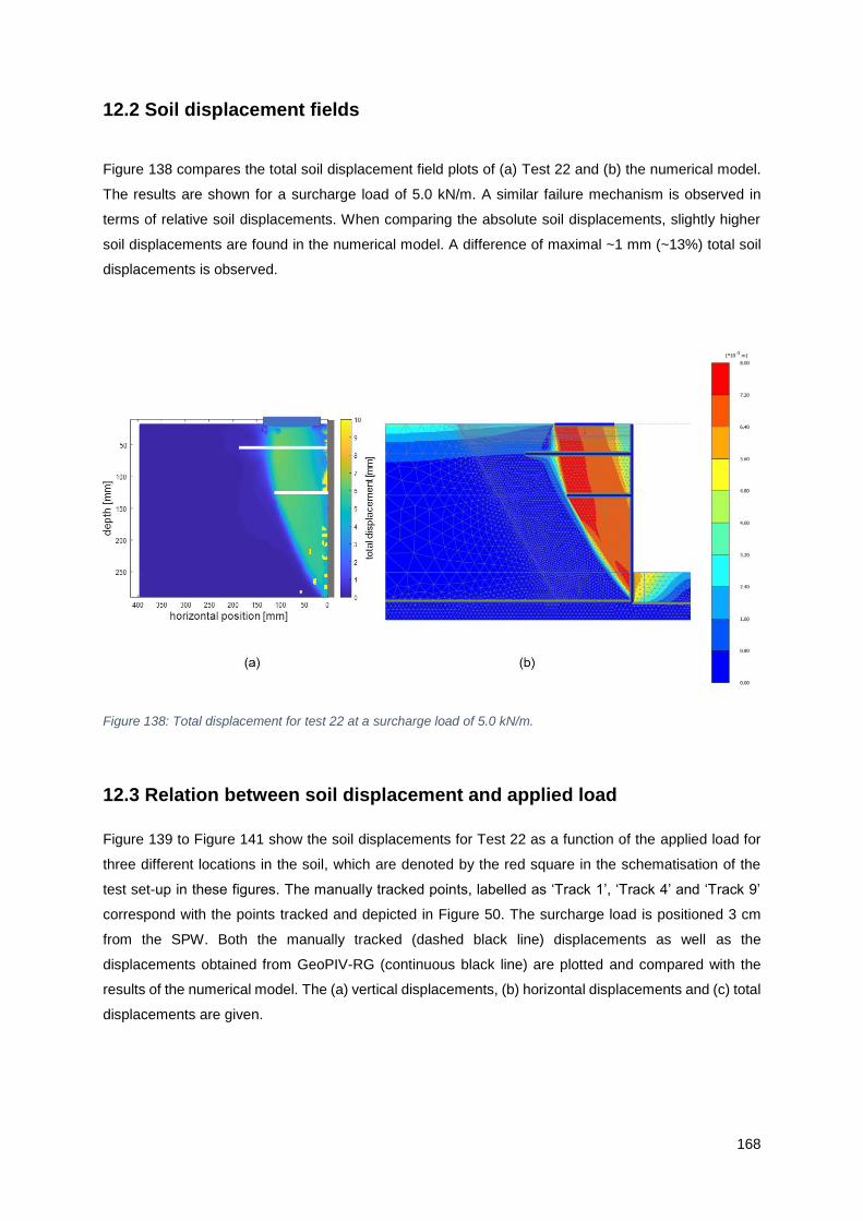
168
12.2 Soil displacement fields
Figure 138 compares the total soil displacement field plots of (a) Test 22 and (b) the numerical model.
The results are shown for a surcharge load of 5.0 kN/m. A similar failure mechanism is observed in
terms of relative soil displacements. When comparing the absolute soil displacements, slightly higher
soil displacements are found in the numerical model. A difference of maximal ~1 mm (~13%) total soil
displacements is observed.
Figure 138: Total displacement for test 22 at a surcharge load of 5.0 kN/m.
12.3 Relation between soil displacement and applied load
Figure 139 to Figure 141 show the soil displacements for Test 22 as a function of the applied load for
three different locations in the soil, which are denoted by the red square in the schematisation of the
test set-up in these figures. The manually tracked points, labelled as ‘Track 1’, ‘Track 4’ and ‘Track 9’
correspond with the points tracked and depicted in Figure 50. The surcharge load is positioned 3 cm
from the SPW. Both the manually tracked (dashed black line) displacements as well as the
displacements obtained from GeoPIV-RG (continuous black line) are plotted and compared with the
results of the numerical model. The (a) vertical displacements, (b) horizontal displacements and (c) total
displacements are given.

169
Figure 139: Test 22 with two geogrids: (a) vertical soil displacements (b) horizontal soil displacements (c) total soil displacements
Figure 140: Test 22 with two geogrids: (a) vertical soil displacements (b) horizontal soil displacements (c) total soil
displacements
Figure 141: Test 22 with two geogrids: (a) vertical soil displacements (b) horizontal soil displacements (c) total soil
displacements

170
The following can be observed from Figure 139 to Figure 141:
• The numerical model overestimates the soil displacements except for the vertical displacements
in point 1, which is located at the depth of the top geogrid close to the SPW.
• At small surcharge loads (<~ 3.5 kN/m), the numerical model significantly overpredicts the soil
displacements, whereafter the results approach each other between a load level of 4 -5 kN/m
due to an abrupt increase in the experimental soil displacements. This ‘abrupt increase’
represents the sliding of the soil mass in the active zone.
• At load levels > ~ 5 kN/m, the difference between the numerical and experimental results
increases again.
• A maximum difference in total soil displacement of 4 mm, i.e. 33%, is observed from point 9.
Figure 142 and Figure 144 show the soil displacements for Test 52 as a function of the applied load for
three different locations in the soil. The SPW is anchored by a 13 cm geogrid which is connected at
5 cm below the top of the SPW. The surcharge load is positioned 3 cm from the SPW. Both the manually
tracked (dashed black line) displacements as well as the displacements obtained from GeoPIV-RG
(continuous black line) are plotted. The experimental results are compared with the results of the
numerical model. The (a) vertical displacements, (b) horizontal displacements and (c) total
displacements are given. The red square in the schematized test set-up gives the location of the plotted
soil displacements.
Figure 142: Test 52 with one 13 cm geogrid : (a) vertical soil displacements (b) horizontal soil displacements (c) total soil displacements.

171
Figure 143: Test 52 with one 13 cm geogrid: (a) vertical soil displacements (b) horizontal soil displacements (c) total soil displacements.
Figure 144: Test 52 with one 13 cm geogrid: (a) vertical soil displacements (b) horizontal soil displacements (c) total soil displacements.
The following can be observed from Figure 142 and Figure 144:
• At small surcharge loads (< ~2.5 kN/m), the numerical model overestimates the soil
displacements.
• At large surcharge loads (> ~2.5 kN/m), the numerical model underpredicts the soil
displacements.
• A maximum difference in total soil displacements of 6 mm, i.e. 27-35%, has been found.

172
12.4 SPW deformations
Figure 145 shows the SPW displacement at different load levels for (a) Test 22 and (b) the numerical
model of Test 22. The SPW displacement in the experiment is derived from the test photos by
automatically tracking points along the SPW based on colour contrast.
Figure 145: SPW displacement at different load levels. Figure a and b show the results of the experiment and the
numerical model respectively.
From Figure 145, the following has been observed:
• Both the experiment and the numerical model show translation of the SPW and more
displacement at the toe of the SPW compared to the top.
• A gradual displacement is observed for the numerical model, while a more abrupt displacement
is detected in the experimental results. In the experiment, the SPW has almost not moved for
loads ≤ 3.3 kN/m. Then, it slides almost 3 mm along the bottom of the box between a surcharge
load of 3.3 kN/m and 4.2 kN/m. After this increase in displacements, a more gradual
displacement is observed at load levels > 4.2 kN/m.
• Larger displacements are found at similar load level in the numerical model. For load levels ≥
3.3 kN/m, a difference of 2-3 mm is observed.

173
Figure 146 shows the SPW displacement at different load levels for (a) Test 52 and (b) the numerical
model.
Figure 146: SPW displacement at different load levels. Figure a and b show the results of the experiment and numerical model respectively.
From Figure 146, the following has been observed:
• Both the experiment and the numerical model show a translational displacement mode.
• At a load of 4.9 kN/m, the experimental results show failure of the SPW by overturning, while
the numerical results show a slight bending of the SPW.
• The difference in horizontal displacement at the toe of the SPW is smaller than 1 mm between
the experiment and numerical model.
12.5 Deformation geogrid-anchorage
Figure 147 and Figure 149 show the results of the deformation of the two-geogrid anchorage of Test 22.
The deformation of the geogrids has been plotted for a load level of 5 kN/m. The deformation of the
geogrids has been derived from the soil displacements computed by GeoPIV-RG and determined by
manually tracking transverse ribs of the geogrid by means of the plugin MTrackJ of ImageJ, as described
in Section 8.3.2. The deformed top and bottom geogrid are compared with the deformed geogrids in the
numerical model. The vertical position of the geogrid is plotted with respect to the initial location. Hence,
the initial location of the geogrid is a horizontal line at a vertical position of 0 mm.
Additionally, the horizontal displacement of the rear end of the top geogrid is plotted against the applied
load for the experiment and numerical model in

174
Figure 148.
Figure 147: Deformed top geogrid of 18 cm at a surcharge load of 5 kN/m.
Figure 148: Horizontal displacement of the rear end of the top 18 cm geogrid.

175
Figure 149: Deformed bottom geogrid of 11 cm at a surcharge load of 5 kN/m.
From Figure 147 - Figure 149, the following has been observed:
• The shape of the deformed top geogrid correspond well between the numerical model and
experiment except for the rear end and front part of both the top 18 cm geogrid-anchor and
11 cm geogrid-anchor.
• The experimental results in Figure 149 show only ~1.5 mm vertical displacements at the rear
end, while the numerical results show the maximum, namely ~6 mm vertical displacement at
the rear end of the bottom 11 cm geogrid-anchor. From the results of Section 9.5, we can state
that the pull-out of the geogrid could not be accurately derived from the soil displacements
results obtained from GeoPIV-RG.
• The numerical model predicts 1 mm larger maximum vertical displacements of the geogrid-
anchors at a similar load level of 5 kN/m, which is an increase of 17-20%.
• Both the numerical and experimental results show that the top geogrid displaces vertically
approximately 1 mm more than the bottom geogrid.
• Although the experimental results of the pull-out displacement are spikier, the trend and
magnitude of the horizontal displacement of the rear end of the top geogrid is more or less
similar for the experimental and the numerical results. A pull-out displacement of almost 6 mm
is computed.

176
Figure 150 shows the experimental and numerical results of Test 52, with one 13 cm geogrid-anchor.
The blue and black colour denote the numerical and experimental results respectively. The continuous
lines and dashed lines are the results at a load level of 2.5 kN/m and 4.9 kN/m respectively.
Figure 150: Deformed 13 cm geogrid-anchor at two different load levels.
From Figure 150, the following can be observed:
• At a load level of 2.5 kN/m, the vertical displacement of the geogrid differ less than 1 mm
between the numerical model and experiment for the middle part of the geogrid.
• At a load level of 4.9 kN/m, the numerical model shows significantly lower vertical displacements
compared to the experiment. A difference of ~10 mm is observed between the maximum vertical
displacements.

177
12.6 Tensile force in the geogrid
This section looks at the tensile force that develops in the geogrid. The tensile force in geogrid layers in
reinforced soils can be calculated analytically with the ´Tie Back wedge’ method, that was adopted by
for example the Dutch design guideline for reinforced soils (CUR198, 2017). The ‘Tie Back wedge’
method calculates the maximum tensile force that is mobilised in a geogrid in reinforces soil. More
details regarding the method can be found in Chapter 3. The tensile force is calculated based on the
analytical design calculation for the mobilised tensile force only. Hence, the tensile force, which could
be maximally mobilised considering the length of the geogrid, is calculated. This seemed to be a fair
assumption as the geogrid was pulled-out at the load level we are analysing. In accordance with the
input parameters of the PLAXIS model, an apparent coefficient of friction - defined by 𝜇𝑝 in CUR198
(2017) – of 0.8 is assumed. The ‘Tie Back wedge’ method also asks for an influence factor (a’bc ) for the
cohesion and a material factor (gm). The first factor is generally determined from laboratory testing and
the second factor is a partial factor whose value depends on the geotechnical category, GC1, GC2 and
GC3 (CUR166, 2008). For a’bc, a value of 1 is assumed. The geotechnical category is out of the scope
of this research. Hence, a value of 1 is assumed for gm . For the approximation of the vertical soil
stresses, the 2V:1H approximation is used to compute the increase in vertical stress due to strip footing
loading. Accordingly, we departed from the proposed Boussinesq’s formulation for the approximation of
the vertical stresses due to strip footing loading. No substantial differences are expected as a
consequence of this simplification.
Figure 151 and Figure 152 show the tensile force distribution for Test 22 along the top geogrid-anchor
of 18 cm and bottom geogrid-anchor of 11 cm respectively. Results are plotted for an applied load of
5 kN/m. This test configuration of Test 22 includes two geogrids of 18 cm and 11 cm. The footing plate
of the surcharge load is position 3 cm from the SPW, so that the inner – and outer edge of the footing
plate are located 3 cm and 13 cm from the SPW. The results of the numerical model (PLAXIS),
experiment (geogrid stiffness x measured strain that was in turn calculated using GeoPIV-RG and
Manual tracked transverse ribs of the geogrid), and the theoretical solution according to the Tie-back
wedge method are given.

178
Figure 151: Tensile force distribution in the 18 cm top geogrid-anchor for Test 22 at an applied load of 5.0 kN/m.
From Figure 151, the following can be observed:
• A similar tensile force of 1.45 kN/m in the anchor point is found with the numerical model and
the Tie Back wedge method.
• The tensile force reduced at a distance > 30 mm from the SPW for the numerical model, while
the Tie Back wedge method shows a tensile force reduction at a distance > 100 mm from the
SPW.
• The experimental results show significantly higher tensile forces at a distance < ~20 mm from
the SPW.
• The tensile force derived from GeoPIV-RG is also very high compared to the theoretical and
numerical results at a distance > ~100 mm from the SPW.
• The tensile force derived from the manually tracked transverse ribs (GeoPIV-RG) is very high
compared to the Tie Back wedge method and numerical results at a distance > ~200 mm and
< ~150 mm from the SPW.
• Along the length of the geogrid between ~40 mm and ~110 mm from the SPW, the experiment
results obtained from the manual tracking show average tensile forces of 25% the magnitudes
computed by the numerical model.
• Along the length of the geogrid between ~50 mm and ~100 mm from the SPW, the experiment
results obtained from the manual tracking show an average tensile force of 55% of the
magnitudes computed by the numerical model. An average tensile force of 0.91 kN/m is
computed by the numerical model for this part of the geogrid.

179
Figure 152: Tensile force distribution along the bottom geogrid-anchor of 11 cm length for test 22 at an applied
load of 5.0 kN/m.
From Figure 152, the following is observed:
• A tensile force of 0.71 kN/m, 0.59 kNn/m and 2.6 kN/m is found for the Tie Back wedge method,
numerical model and experiment at the anchor point.
• The tensile force distribution of the numerical model and the Tie Back wedge method looks very
similar. The numerical model shows on average 26% lower tensile forces compared to the
theoretical solution along the first 70 mm length of the geogrid. For the last 40 mm of the geogrid,
the tensile forces correspond very well.
• The experimental results show significantly lower values compared to the theoretical solution
and numerical results along the first ~40 mm of the geogrid, except for a local point at ~20 mm
and at the connection with the SPW. At ~20 mm distance from the SPW, the experimental
results come close to the values computed by the numerical model, which calculated a tensile
force of ~0.5 kN/m.
• Between ~50 and ~70 mm length of the geogrid, similar tensile forces are found from the
theoretical, experimental and numerical results. The average tensile force along this part of the
geogrid is 0.55 kN/m for the numerical model.
• At a distance > 80 mm from the SPW, the experiment shows significantly higher values than the
numerical model and theoretical solution.

180
Figure 153 shows the experimental and numerical results of the tensile force distribution for the 13 cm
geogrid-anchor of Test 52 at a load level of 4.9 kN/m.
Figure 153: Tensile force distribution along 13 cm geogrid-anchor at a load level of 4.9 kN/m.
From Figure 153, the following can be observed:
• The experiment shows a very fluctuating distribution. Along the first 20 mm and last 70 mm of
the length of the geogrid unrealistically high tensile forces are computed.
• The numerical model shows a tensile force of 1.73 kN/m at the anchor point. The tensile forces
reduces at a distance > 46 mm from the SPW.

181
12.7 Analysis and discussion
12.7.1 Failure mechanism
The total soil displacements and critical slip surface obtained from the experimental and numerical
results agree very well. Figure 138 shows that the largest soil displacements occur underneath the
second half of the loading plate, i.e. between the centre and the outer edge of the loading plate. The
larger displacements can be explained by the fact that the footing plate was allowed to move freely. As
a consequence, more load was distributed to the second half of the plate. The soil displacements around
the geogrids indicate that the soil behind the critical slip surface is activated by the geogrids. This implies
that the geogrid moves through the soil and the pull-out mechanism has started.
Both the experimental and numerical results show a secondary slip surface from the inner edge of the
footing plate to the SPW. The intersection point of the secondary slip surface with the SPW cannot be
derived from the experimental results for a load position of 3 cm from the SPW, but can be derived from
the experimental results for a load position of 13 cm from the SPW. However, the secondary slip surface
was not fully developed in the numerical model. Accordingly, the similarity of the shape of the secondary
slip surface between the numerical and experimental results cannot be investigated fully. We can only
conclude that the secondary slip surface initiates at the inner edge of the footing plate for both the
experimental and numerical model.
The theoretical slip surfaces of the CUR166 (2008) and the Tie Back wedge method of CUR198 (2017)
do not correspond with the critical slip surfaces observed in the experimental and numerical results.
These theoretical approximations do not yet take into account the influence of the surcharge load. The
critical slip surface is clearly defined by the position of the footing plate of the load. Ohde’s design
calculation gives the best approximation as it assumes a critical slip surface starting at the outer edge
of the footing plate. According to Ohde’s approximation, the critical surface would intersect the SPW at
a depth of 306 mm and 542 mm for a footing plate of 100 mm length positioned 30 mm and 130 mm
from the SPW. The limited height of the SPW modelled in the experiment disrupts the failure
mechanisms at the bottom of the test box. Hence, critical slip surfaces approximated by theoretical
methods cannot be compared with the experimental and numerical results for load positions >27 mm
from the SPW.

182
12.7.2 Relation between soil displacement and applied load
The main findings from Figure 139 - Figure 141 for the test configuration with the two-geogrid anchored
SPW and the load positioned 3 cm from the SPW (Test 22):
• Up to an applied load of 3.5 kN/m, the numerically calculated total soil displacements are a
factor 2 and 3 higher than the total soil displacements in the experiment for a point in the soil
close to the SPW at the depth of the top geogrid and bottom geogrid respectively.
• The total soil displacements correspond best at an applied load of 4-5 kN/m
• At loads > 5 kN/m, the total soil displacements start to deviate again more. Again, the total soil
displacements of the numerical model are larger than the total soil displacements of the
experiment.
• The general difference between the numerical and experimental results is characterized by an
overestimation of the total soil displacements by the numerical model. Only the vertical
displacements for the point at the depth of the top geogrid are significantly larger in the
experiment compared to the numerical model at loads > ~3.5 kN/m.
The larger displacements in the numerical model may be a consequence of the following:
• The correction method applied to the numerical model to correct for the sidewall friction in the
experiment.
The reduction of the vertical stresses in the soil due to sidewall friction should be compensated
by the zero soil weight in the numerical model. This correction may lead to ‘overcorrection’ at
lower surcharge loads and ‘undercorrection’ at higher surcharge loads. Only the overestimation
at loads > 5 kN/m may be clarified by inaccurately correcting of the vertical stresses.
• The friction between SPW and bottom of the test box as well as the silicone block and bottom
of test box.
Figure 145 shows larger SPW displacements in the numerical model compared to the
experiment. This could indicate that the friction between the SPW and the test box is
underestimated. Higher soil displacement will be a consequence of the larger SPW
displacements.
• The densification procedure during the experiment .
The overestimation of the soil displacements at loads < 3.5 kN/m may be the result of an
underestimated initial void ratio and/or K0 value. During the experiment, the sand was densified
up to surface level. A plausible explanation would be that the soil is to some degree
overconsolidated. The relatively higher stiffness and strength properties of the top soil layer will
result to less displacement and sliding of the soil mass at relatively higher loads.
• The connection of the geogrid to the SPW
The connection of the geogrid to the SPW may clarify the higher vertical soil displacements in
Figure 139a at a load > ~ 3.5 kN/m. The SPW starts to displace significantly between a load
level of 3.3 – 4.2 kN/m as can be observed from Figure 145a. The moment the SPW starts to
slide forward, the geogrid has to be pulled tight first before tensile force can be mobilised.

183
During the preparation of the experiment, it was difficult to pull the geogrid tight while pouring
sand on top of it. This gives a plausible explanation for the jump in vertical displacement the
moment the SPW starts to displace. In practice, geogrids are pre-stressed when they are used
as anchorage for SPWs. Hence, the importance of pre-stresses is demonstrated by the
difference in vertical soil displacements between the experiment and numerical model.
• One centimetre difference in vertical distance between loading plate and top geogrid.
Because the depth of the soil layer differs 1 cm between the experiment (29 cm depth) and
numerical model (30 cm depth), the soil layer above the top geogrid in the experiment has a
thickness of 4 cm compared to the thickness of 5 cm in the numerical model. For comparison
of the soil displacement-load curves for the three locations in the soil domain, it was decided
to keep the vertical distance relative to the top geogrid equal between the experiment and
numerical model. When we consider point 4, this location in the soil is closer to the loading
plate in the experiment compared to the numerical model. Accordingly, relatively larger vertical
displacements would be expected from the experimental results in point 4. However, the
opposite relation has been observed in Figure 140. Moreover, a maximum difference of 0.5 mm
vertical displacement was observed if the experimental results were plotted for a 1 cm lowered
or elevated vertical position of point 4. Concludingly, the difference in soil depth will not clarify
the difference in soil displacements.
Next, the experimental and numerical results were compared for a 13 cm geogrid-anchor at the load
positioned 3 cm from the SPW (Test 52), see Figure 142 and Figure 144. The numerical model
overestimates the soil displacements significantly at loads > 2.5 kN/m. The absolute difference
increases with increasing load level. Since these findings are not in line with the overestimation of the
soil displacements at higher loads for Test 22, it is difficult to understand what is happening. It may be
that there are factors playing a significant role in the experiment which have not been included or cannot
be included in the model. It may be that these differences are caused by certain input parameters or
other modelling choices for the numerical or physical model.
It can be hypothesized that the large difference in experimental and numerical soil displacements are
caused by the way the geogrid is modelled. Since the geogrid is modelled as a line element, the
interaction mechanisms cannot be simulated perfectly. The main difference between the line element
and the geogrid is that the apertures and transverse ribs are not included in the model. It may be
possible that the interaction mechanisms that play a role in the friction mobilised along the geogrid within
the active zone are less well simulated than the pull-out mechanisms. In case of a geogrid of only 13
cm, which has no length outside the active zone, it may be that these discrepancies lead to larger
differences between experiment and model than in case of a geogrid of 18 cm length.

184
Other modelling choices which may be of relevance regarding the differences in soil displacement are:
• The use of the Hardening Soil model to model the soil behaviour. It would be interesting to
compare the results with a model that uses the Hardening soil model with small-strain stiffness
(HSsmall).
• The mesh has not been updated between the calculation phases. It would be interesting to
compare the results with a model that updates the mesh. At overturning of the SPW and
differential vertical displacement along the length of the geogrid, it may be that errors arise in
the computation of the SPW displacements and deformation of the geogrid if second order
effects are not included.
12.7.3 SPW deformations
From Figure 145 and Figure 146, it is observed that the numerical model overestimates the SPW
displacements for the double-anchored SPW (Test 22), and the SPW with a 13 cm geogrid-anchor
(Test 52), except for the larger load levels in Test 52. SPW displacements are underestimated by the
numerical model when the SPW starts to overturn.
The difference in soil displacements between the numerical model and experiment are in line with the
overestimation and underestimation of the SPW displacements for Test 22 and Test 52 respectively.
We can argue that the difference may partly be a result of second order effects, which have not been
included in the numerical model. The SPW fails by overturning for Test 52. It may be that the rotation of
the SPW around its toe is underestimated by the numerical model, because the mesh has not been
updated.
12.7.4 Deformation geogrid-anchorage
Test 22: double geogrid-anchored SPW
At an applied load of 5 kN/m, the numerical model overestimates the vertical displacement of both the
top and bottom geogrid by approximately 1 mm, see Figure 147. Both the experiment and numerical
model show that the vertical displacement of the top geogrid is approximately 1 mm larger than the
vertical displacement of the bottom geogrid. The differences in vertical displacements of both geogrids
are in line with the differences in vertical soil displacements in Figure 139a and Figure 141a. The
deformation of the geogrid deviates more in the front and end part of the geogrids. This can be explained
by the inaccuracy of the manually tracked transverse ribs. Close to the SPW and at the intersection with
the critical slip surface soil covered the transverse ribs adjacent to the transparent sidewall (almost)
completely.

185
Test 52: single geogrid-anchored SPW with a geogrid length of 13 cm
The deformed geogrid was compared for two load levels consciously; at a load level of 2.5 kN/m the soil
displacement-load curves between the numerical and experimental results agreed well, while at a load
level of 4.9 kN/m the numerical model overestimated the soil displacements significantly, see Figure
142. Indeed, this can also be observed from the results of the deformed geogrid in Figure 150. At a load
level of 2.5 kN/m, the vertical displacements between the numerical and experimental model differ less
than 1 mm for the middle part of the geogrid. The results only deviate more at the front and rear end of
the geogrid. In the rear end of the geogrid, it seems that the geogrid in the experiment is hold in place
more effectively by the soil behind the critical slip surface in the experiment compared to the numerical
model. A similar deviation was observed in the end part of the bottom 11 cm geogrid of the double
geogrid-anchorage. At a load level of 4.9 kN/m, the difference in maximum vertical displacement is
~10 mm. A more or less similar difference in vertical soil displacement is observed in Figure 142a.
12.7.5 Tensile force distribution along the geogrid
A difference of approximately 1 mm vertical displacement is observed in the deformation of the geogrid-
anchorage between the experimental and numerical model for the two-geogrids anchorage of Test 22
at a load level of 5 kN/m, see Figure 147. For this load level, we could presage a slightly lower tensile
force distribution along the geogrid in the experiment. The experimental, numerical and theoretical
results are compared for the top and bottom geogrid-anchor of the double geogrid-anchored SPW in
Figure 151 and Figure 152 at a similar load level of 5 kN/m. Chapter 7 elaborated on the derivation of
the strain and tensile force along the geogrid from the experiment. Hereby, the reliability of the tensile
force distribution derived from the soil displacements obtained from GeoPIV-RG was questioned. Since
we were not able to compute the soil displacements within the small shear band around the geogrid,
apparently high tensile forces were measured at the location of the critical slip surface and in the part of
the geogrid outside the active zone. Also, the accuracy of the methods used to compute the tensile
forces from the experimental results is mentioned as the cause of high tensile forces close to the SPW
and at the location of the critical slip surface. From Figure 151 and Figure 152, it can be observed that
the numerical results give significantly lower – more plausible – tensile forces at the location of the
critical slip surface and close to the SPW. The experimental results obtained from the manually tracked
geogrid are in the same order of magnitude along the remaining part of the geogrid. For the middle part
of the geogrids, average tensile forces of 0.91 kN/m and 0.55 kN/m were computed by the numerical
model for the top and bottom geogrid respectively. The Tie Back wedge method finds tensile forces of
magnitudes close to the numerical results. However, Figure 151 shows that the distribution of the tensile
forces differs along the top geogrid. It can be concluded that the Tie Back wedge method is based on
two assumptions which conflict with the results of the numerical model:
• The Tie Back wedge method assumes no transfer of tensile force to the soil inside the active
zone, whereas the numerical model demonstrates that the soil enclosed by the SPW and critical
slip surface (active zone) provide some resistance.
• The Tie Back wedge method assumes a critical slip as defined by Mohr Coulomb and relates
the mobilised friction along the geogrid to the intersection point with the slip surface. The

186
numerical model has shown in Chapter 9 that the mobilised frictional forces along the geogrid
depend on the position and length of the loading plate, because those determine the location
of the critical and secondary slip surface at surface level. Since the theoretical and numerical
slip surfaces do not correspond, different tensile forced distributions will be calculated.

187
13 Discussion & Conclusions
Chapter 6 to 9 presented and analysed the small-scale experiments. Some of the test configurations
were simulated using a plane strain numerical model (PLAXIS, Chapter 10) and the results were
analysed in Chapter 11 and compared with the experimental results in Chapter 12. Based on the findings
described in Chapter 9, 11 and 12, the research questions will be answered in Section 13.3. Before the
research questions as defined in Chapter 1 will be answered, two additional research questions came
forward from:
• the method used to correct for sidewall friction in Chapter 10.2, and
• the method used to derive the tensile strain in the geogrid from the experiment in Chapter 8.3.
The research questions based on Chapter 10.2 and Chapter 8.3 respectively are as follows:
• How well can sidewall friction be included in a 2D numerical model?
• Can DPIV be used for the derivation of the tensile strain in the geogrid?
These two research questions will be answered first in Section 13.1 and 13.2.
Conclusions are drawn in Section 13.4. Finally, we have made a proposal from the conclusions for the
analytical design calculation for the mobilised resistance along the geogrid-anchorage in section 13.4.
13.1 How well can sidewall friction be included in a 2D numerical model?
The advantage of a 2D PLAXIS model over a 3D PLAXIS model is that higher accuracy can be achieved
with 2D elements compared to 3D elements. Furthermore, computational costs will be reduced.
However, the drawback of not having the possibility to include sidewall friction while simulating the small-
scale tests is in our case larger than the benefits of a 2D numerical model. Referring to the analytical
relations proposed by Jewell (1987) and Bathurst and Benjamin (1987), the sidewall friction will increase
non-linearly with depth due to:
(1) increased soil weight;
(2) the additional friction due to the strip footing load (arching effect).
As a consequence, vertical and horizontal soil stresses are attenuated more with depth. The arching
effect will result in larger attenuation of stresses in the soil directly below the loading plate relative to
the sides. Hence, a correction factor is required in numerical simulations, which is a function of:
• the applied load;
• the depth;
• the distance from the loading plate;
• the distance from the front and the back wall;
The arching effect in the soil between the sidewalls may result to a correction factor, which should be a
function of the in-plane direction also. However, in our case, the width of the test box is very narrow and

188
we can assume that the sidewall frictional forces will have equal influence along the entire cross-section
of the test box.
Since it is not possible to incorporate such a correction factor in a 2D PLAXIS model, a deviation
between the soil stresses in the experiment and the numerical model at similar load level could not be
avoided. By manipulating the unit soil weight in the 2D PLAXIS model, it was attempted to simulate the
soil stresses at the maximum load level reached during the experiment as closely as possible. The unit
soil weight was reduced by a correction factor to account for the attenuated soil stresses due to sidewall
friction.
The derivation of this correction factor was based on:
• the relations of Jewell (1987) and Bathurst and Benjamin (1987),
• the measured interface sidewall friction angle (𝛿) derived from the Pull-up test (see
Section 7.2.2)
• the measured average sidewall friction force at the bottom of the box (see Section 7.2.3)
Based on the results of Section 10.2.5, we can state that this correction method leads to good agreement
with the vertical stresses which are attenuated by sidewall friction. Acceptable small differences between
the soil stresses in the experiment and numerical model can be obtained for load levels between 3 and
6 kN/m if the soil weight is reduced to zero. However, the soil weight is underestimated too much due
to the manipulation of the soil weight when the surcharge load level is < 2.5 kN/m. As a consequence,
the stress path of the soil will deviate too much from the experiment for these low surcharge loads.
We applied only one reduction factor to the entire soil domain as we only measured the average weight
reduction along the entire bottom of the box (see Section 7.2.3). In case the surcharge load is close to
the SPW, one reduction factor may suffice as the soil zone of influence will be all below or near to the
loading plate. However, probably a lower reduction factor is required for the soil close to the SPW relative
to the reduction actor below the loading plate.
Concludingly, we can include the dependency of the correction factor on the distance from the loading
plate – to some degree - by dividing the soil in different zones with different unit weights. However, we
cannot include the dependency of the correction factor on the applied surcharge load. The stress paths
developing during the test cannot be simulated correctly. Another problem is that the reduction in vertical
stresses is limited to the self-weight of the soil. For surcharge loads > 6 kN/m, reducing the weight of
the soil cannot offset the frictional forces in the experiment. For higher load levels, one must consider
to add point loads in the soil domain, which act in upward direction and which magnitude increases with
depth.
It is interesting to evaluate the possibilities of including the sidewall friction in a 2D model. However, it
can be concluded that you cannot simulate sidewall friction well in a 2D PLAXIS model. Moreover, it will
become a cumbersome model. For the sake of simulating the experiment by a numerical model, either
a wider test box is required to make the influence of the sidewall friction negligible or a 3D model needs
to be validated first for which the sidewall can be modelled.
189
13.2 Can DPIV be used for the derivation of the tensile strain in the geogrid?
Whether DPIV can be used to derive the tensile strain in the geogrid depends on:
• The presence of interparticle locking due to the interaction of the soil with the geogrid.
• The fraction of geogrid surface area that is solid and in contact with the soil (𝛼𝑑𝑠).
• The minimum required interrogation window size (or subset size) used by DPIV.
As explained in section 3.1.2, the tensile strain in the geogrid can generally be mobilised in two ways:
• by shear between soil and the geogrid;
• by shear between soil-soil.
Shear between soil and geogrid will occur if the grains are significantly smaller or larger than the aperture
size of the geogrid. The shear zone will be along the geogrid. Shear between soil-soil will occur if the
grains just fit in the apertures of the geogrids. As a consequence, the grains in the apertures will move
along with the geogrid and will shear with the grains just above and below the geogrid. The shear zone
will be just above the geogrid.
DPIV computes the displacements of subsets of soil. The minimum size of these subsets depends on
the resolution of the digital test photos, the image texture quality and particle diameter (see Section 8.1).
First of all, the assumption must hold that the soil adjacent to the geogrid and the geogrid displaces as
one in order to use DPIV to compute the tensile strains in the geogrid. Cardile et al. (2017) demonstrated
that complex failure mechanisms develop in the soil in the apertures of the geogrid under pull-out
mechanisms. Since a geogrid-anchor experiences pull-out mechanisms, it is not likely that the
assumption holds for relatively small grains with respect to the aperture size of the geogrid. If the ratio
of the grain size to the aperture of the geogrid is close to 1, it is likelier that the grains in the apertures
and the geogrid move as one.
Second, the shear band of soil must be sufficiently thick – i.e. larger than the interrogation window size
(or subset size) used by DPIV – in order to capture the soil displacements in this shear band by means
of DPIV. Generally, the larger the grain size, the larger the shear band. Particle interlocking will widen
the shear band. In case the grains just fit in the apertures of the geogrid, a shear zone will develop
above the geogrid. The displacement of the bottom part of this shear zone adjacent to the geogrid may
be used to derive the tensile strain in the geogrid.
For our experiments, no reliable tensile strains in the geogrid were derived from the DPIV soil
displacement results by means of the calculation procedure described in Section 8.3.1. The transverse
ribs of the geogrid are less than 0.5 mm thick. The minimum subset size of 3.2 mm, which was required
to obtain accurate results from DPIV, was too large to track the transverse ribs and thin shear band
along the geogrid by means of DPIV.
Another problem was that the soil covered the transverse ribs, which were visible on the test photos at
the beginning of the test, more and more as the soil deformation increased. Especially, the rear part of

190
the geogrid was poorly visible after some soil deformation. If the pixel pattern of the subsets of soils,
tracked by DPIV, alter largely, the cross-correlation technique used by DPIV will not lead to accurate
results.
13.3 Answers to the research questions
13.3.1 What relation can be found between the (length of) the geogrid-anchorage and the shape and size of the critical slip surface?
Both the experimental and numerical results have demonstrated that the geogrids will influence the
shape and size of the critical slip surface in case of intersection. The experimental results show that
when the initially straight slip surface intersects with the geogrid, the slip surface reorients vertically.
Due to the resulting perpendicular crossing of the critical slip surface at the intersection with the geogrid,
the shape of the slip surface becomes more curved and wider. This results in a longer path of the slip
surface, resulting in an increase of the shear resistance of the soil along the slip surface and more
bearing capacity. These findings are in accordance with (Ziegler, n.d.) and (Jacobs et al, 2016).
13.3.2 How does the surcharge load position affect the mobilised anchor force?
The position of the surcharge load plays a key role in the mobilisation of tensile forces along the geogrid.
The tensile force distribution depends on the developed slip surfaces. The slip surfaces are defined by
the position and length of the loading plate, because the failure mechanism is driven by the surcharge
load. The critical slip surface initiates at the outer edge of the loading plate. A secondary slip surface
develops at the inner edge of the footing plate. The magnitude of the mobilised anchor force depends
on the length of the geogrid outside the critical slip surface. The active zone enclosed by the two slip
surfaces is resisted to slide along the slip surface by the tensile force mobilised in the rear part of the
geogrid behind the active zone.
Besides the load position, the length of the loading plate is thought to be of importance with regard to
the mobilised tensile force in the geogrid. From the numerical results, it was observed that the largest
share of the resistance was mobilised along the bottom of the geogrid within the active zone. Since the
length of the loading plate defines the distance between the secondary and critical slip surface - and
accordingly the width of the active zone - we presume that the mobilised anchor force is also a function
of the length of the loading plate.

191
13.3.3 What interaction mechanism(s) describe the development of the resistance along the geogrid-anchor(s)? What is the influence of the length of the geogrid on the mobilised anchor force?
From the experimental results, three main conclusions can be drawn:
1. The connection of the geogrid to the SPW plays a significant role in the mobilisation of
tensile force along the geogrid and transfer of vertical pressures via the geogrid to the SPW.
Without connection, no resistance is provided by the part of the geogrid within the active
zone.
2. The intersection of the geogrid with the critical slip surface plays a significant role in the
mobilisation of tensile force along the geogrid.
3. The confining effect of the geogrid as a consequence of the surcharge load above the
geogrid turns out to be insignificant with regard to the stability of the soil behind the SPW.
Interaction mechanism(s) related to point 1:
The lateral pressure against the SPW increases due to the surcharge load and as a result, the SPW
starts to either slide along the bottom box or turn around its toe. Due to the moving SPW, space behind
the SPW increases and soil starts to slide along the critical slip surface downward and laterally towards
the toe of the SPW. This will affect the geogrid in two ways: the SPW pulls in one direction, while the
moving soil mass tries to drag the part of the geogrid within the active zone downward.
The fixity of the geogrid at the anchor point results in a relative displacement between the geogrid and
soil within the active zone. From the experimental results, we can conclude that the SPW will fail by
overturning in case of no or short (6-13 cm length) anchorage. The longer the geogrid, the more
resistance against overturning. Accordingly, it can be argued that the initial interaction between the soil
and geogrid within the active zone is a pull-out mechanism. However, the pull-out mechanism will not
be the only mechanism involved. The geogrid will act as a kind of barrier net. The sand tries to push the
geogrid downward at the contact with the solid geogrid and tries to go through the apertures of the grid.
The rough interface of the solid geogrid makes that the grains cannot move easily through the apertures.
Shear stresses between the geogrid, grains within the apertures and grains along the length of the
geogrid are mobilised. Apparently, within the active zone, most friction is mobilised along the bottom of
the geogrid – as was observed in the numerical results.
Interaction mechanism(s) related to point 2:
The interaction mechanism related to the intersection of the geogrid with the critical slip surface can be
related best to a direct (or simple) shear test. The slip surface cuts the initially horizontal geogrid with a
certain angle. The tensile force acting across the slip surface i.e. the surface of maximum stress obliquity
in the soil, increases the shear resistance along the critical slip surface. We assume that the magnitude
of the resisting tensile force is defined by the pull-out resistance of the part of the geogrid behind the
critical slip surface.

192
Interaction mechanism(s) related to point 3:
Our experimental results show that the influence of the confinement effect of the geogrids is negligible.
No increase in bearing capacity was observed in the load-displacement curves of non-connected
geogrids with a length too small to intersect with the critical slip surface. Since the confining effect of the
geogrid should not depend on the connection of the geogrid to the SPW, we can conclude that the
confining effect is no dominant interaction mechanism. Increased soil resistance was observed when
the non-connected geogrid intersected with the critical slip surface. The local increase of strength at the
intersection of the critical slip surface with the geogrid can be seen as some horizontal confinement,
because the slip surface continues its path vertically.
13.3.4 In case of multiple geogrid-anchors, do they influence the mobilised anchor force of each other?
Since we could not rely on the experimental results of the mobilised tensile force in the geogrid, this
conclusion is based on the numerical results only. We compared the tensile force distribution of a single
and double anchored SPW. Both models included a top 18 cm geogrid-anchor. The double anchored
SPW had a second 11 cm geogrid-anchor at 7 cm vertical distance from the top geogrid. Lower anchor
forces were found in the 18 cm geogrid-anchor when a second geogrid-anchor was included. The bottom
geogrid-anchor provides part of the resistance, which results in 10% to 11% lower anchor forces in the
top geogrid (see Figure 129 in Section 11.2.4) . Less well understood, is the difference observed in the
tensile force distribution along the top 18 cm geogrid-anchor at approximately the location of the
intersection with the critical slip surface (between ~115 and ~130 mm distance from the SPW). It can
be observed that the tensile force remains more or less constant for the test with the two-geogrid
anchorage, while it increases for the test with the top 18 cm geogrid only. This means that friction is
mobilised along this part of the geogrid in case there is no second bottom geogrid and is not mobilised
in case there is a second bottom geogrid. It is thought that the difference in tensile force distribution has
to do with the alteration of the shape and width of the critical slip surface by the intersection of the slip
surface with the bottom geogrid-anchor. If the slip surface has widened due to the interaction with the
second bottom geogrid, the soil between ~115 and ~130 mm distance from the SPW may be activated
already and cannot provide any resistance at the top 18 cm geogrid.
13.3.5 How does the numerically modelled geogrid-anchor behave in accordance with the experimental findings?
We cannot investigate how well the numerical model simulates the interaction between the geogrid and
soil based on the tensile force distributions, because we could not rely on the experimental results of
the tensile force distribution along the geogrid. However, we can compare the failure mechanism, soil
displacements, SPW displacements and deformation of the geogrid(s).
The experiment and numerical results show a very similar shape and size of the critical slip surface. The
secondary slip surface was also observed in both. Both demonstrated that the geogrids influence the

193
shape and size of the critical slip surface at the intersection. These findings imply that the numerical
model simulates the soil-geogrid interaction well.
Based on the experimental and numerical soil displacements of Test 22 and Test 52, it can be concluded
that the numerical model does not simulate the small-scale experiment perfectly. At higher load levels,
soil displacements were overestimated for Test 22, while soil displacements were underestimated for
Test 52. The differences in SPW displacement between the numerical model and experiment are in line
with the differences in soil displacement. Especially, the trend of the load-displacement curves and
relative displacements within the entire soil domain are important indicators with regard to the degree
of similarity in soil-geogrid interaction. The soil displacement fields look very similar. However, the load-
displacement curves show different behaviour. The way the geogrid is modelled in the numerical model
may be (part of) the cause of these discrepancies.
When the deformations of the geogrids were studied at a load level at which the load-displacement
curves fit best, it was found that the maximum vertical displacement and pull-out displacement of the
rear end of the geogrids agreed quite well. The similarity between the vertical displacement and pull-out
displacement of the geogrid gives trust in the correctness of the numerical model with regard to the
simulation of the geogrid-soil interaction.
Doubts in the correctness of this geogrid model came mainly forward from the findings of Lees (2014).
Lees (2014) argues that the influence zone of the geogrid is larger than just the thin layer of sand
particles adjacent to the geogrid. If the geogrid is modelled as a 1D tensile element, this influence zone
cannot be taken into account and the confining effect of the geogrid is underpredicted. Concludingly, if
the confining effect of the geogrid - i.e. the increase in soil shear resistance by the restraint horizontal
displacements of the soil around the geogrid - is no dominant interaction mechanism, the modelling of
the geogrid as a 1D tensile element can be justified. Figure 84shows that the geogrid-anchors of a length
of ≤ 13 cm do not provide resistance if they are not connected to the SPW. We would have expected to
observe higher failure loads for the non-connected geogrids ≤ 13 cm with the surcharge load positioned
above the geogrids, if the confining effect would have played a role. From the findings of Figure 84, it
can be argued that the confining effect of the geogrid is no dominant interaction mechanism and the
geogrid-soil interaction can be simulated accurately by a 1D tensile element.
Since the geogrid was not pulled completely straight in the experiments – especially at the connection
with the SPW – , relatively higher vertical soil displacements were found at the start of the experiment
compared to the numerical results (see Figure 139a). This finding emphasizes the importance of pre-
stresses the geogrid-anchorage in field.

194
13.4 Conclusions
Geogrid-anchorage of sheet pile walls is a relatively new application of geogrids, in which sheet pile
walls are anchored with one or more layers of geogrid. This type of sheet pile anchorage has some
advantages like low costs and flexibility. This research focusses on geogrid-anchored sheet pile walls
under strip footing loading. A series of small-scale experiments and 2D numerical simulations of these
experiments were conducted and analysed as a first step towards the formulation of an analytical
design-method for geogrid-anchored sheet pile walls.
This research has brought us to a better understanding of:
• the interaction mechanisms: how does the geogrid-anchor mobilise resistance?
• the parameters: which parameters affect the mobilised resistance of the geogrid-anchor?
The following parameters were investigated in the small-scale experiments: the load position, the length
of the geogrid-anchor, and the number of geogrids. The following conclusions concerning the influence
of these parameters were drawn:
• The surcharge load drives the SPW system to failure. A critical slip surface develops from the
outer edge of the loading plate to the toe23 of the SPW. A secondary slip surface develops from
the inner edge of the footing to the SPW. The secondary slip surface and critical slip surface
divide the soil in three different strain fields: zone I (enclosed by the secondary slip surface and
SPW), zone II (the active zone: enclosed between the secondary and critical slip surface) and
zone III (behind the active zone).
• The position of the loading plate with respect to the geogrids is of large influence of the
mobilisation of friction along the geogrid. The position of the loading plate has a decisive
influence: it determines the location where the slip surfaces develop with respect to the position
of the geogrid, and whether the slip surfaces will intersect the geogrids.
• The width of the loading plate defines the width of the active soil zone: it determines the part of
the geogrid which lies within the active zone and the friction mobilised along this part
accordingly.
• The slip surface reorients vertically at the intersection of the critical slip surface with the
geogrids, – as was found by (Ziegler, n.d.) and (Jacobs et al, 2016) also. This results into a
wider and curved slip surface. The increased shear resistance of the soil along the longer path
of the slip surface results to increased stability of the SPW system.
• The confining effect of the geogrid is the mechanism that the geogrid increases the shear
strength of the soil by providing frictional restraint against lateral soil deformations. This effect
is mentioned as one of the interaction mechanisms in the design guideline for reinforced soils
(CUR198, 2017). However, the experiments show that this confining effect – due to the load
positioned above the geogrids - does not contribute to the total resistance.
23 Only ~30% of the total embedment of the SPW is modelled. Therefore, the ‘toe’ of the SPW is actually located ~30% of the
total height of the SPW above the actual toe of the SPW.

195
• The length of the geogrid – as expected – affects the mobilised resistance along the geogrid.
The longer the geogrid, the more resistance is mobilised along the geogrid.
• When the number of geogrids increases (from one to two geogrids), the deformation reduces.
The shape of the critical slip surface is also influenced by the second geogrid-anchor. For the
relatively short second geogrid-anchor, it is found that the slip surface reorients such that the
slip surface becomes wider and circumvents the geogrid.
• The position of the loading plate with respect to the geogrid, the width of the loading plate, the
length of the geogrid and the number of geogrids all have an important role in the development
of the slip surfaces and the resistance that can be developed by the geogrid-anchors. Therefore,
these parameters should be included in the analytical design calculations for the mobilised
tensile force along the geogrid.
Different interaction mechanisms dominate along different parts of the geogrid. The following
conclusions concerning these interaction mechanisms were drawn:
• From both the experimental and numerical results, it was found that the dominant interaction
mechanisms are:
o the membrane effect at the front part of the geogrid (zone I);
o the sliding resistance in zone II and at the intersection with the critical slip surface
(zone II-III)
o the pull-out resistance along the part of the geogrid behind the active soil zone
(zone III)
• For increasing surcharge loading, an increase in soil deformations is followed by the
mobilisation of an additional resistance. This increase may be explained by the sliding soil mass
in the active zone (zone II), that drags along the geogrid downward in the active zone, while the
geogrid parts in zone I and III are hold in place by the SPW and the soil respectively. The geogrid
therefore ends up in a kind of hammock-shape. This gives the membrane effect, in which
vertical soil pressures are transferred via the geogrid to the SPW and the soil in zone III.
• The friction mobilised in the active zone (zone II) is related to the surcharge loading and the
connection with the SPW. The downward soil displacement is resisted by the geogrid due to the
rough interface between the soil and geogrid in the active zone and the resisting force provided
by the SPW. The soil in the active zone tries to push the geogrid downward: shear stresses and
normal stresses will act along and on the transverse and longitudinal ribs of the geogrid. This
mechanism describes a sort of sliding resistance of the geogrid in the active zone (zone II).
• Due to the resistance against downward displacement of the geogrid in the active zone -
provided by the rear part of the geogrid behind the active zone (zone III) - tensile forces are
developed in the geogrid at the intersection of the slip surface with the geogrid. At the
intersection (zone II-III), the tensile force in the geogrid provides sliding resistance against the
sliding soil mass in the active zone (zone II).
• The friction along the rear part of the geogrid (zone III) is mobilised due to the displacement of
the geogrid relative to the soil. The displacement of the geogrid is the consequence of two

196
mechanisms. First, the geogrid will be pulled out of the soil by the SPW, which displacement
increases at increasing surcharge load. Second, the geogrid will be pulled out by the sliding soil
mass in the active zone (zone II). This friction mobilised along the geogrid is referred to as the
pull-out resistance.
• From the numerical results, it is concluded that friction is mainly mobilised along the top of the
geogrid in zone III (behind the active zone), and along the bottom of the geogrid in zone II (active
zone). At a settlement of the geogrid of ~7 mm, approximately 40% and 60% of the total
resistance is provided by the frictional force of the soil along the top and bottom of an 18 cm
geogrid respectively. No friction is mobilised along the geogrid in zone I.
• Based on the numerical results, the frictional resistance is mobilised as follows:
o in zone I: no shear resistance is provided by the soil
o in zone II (the active zone): the friction along the bottom interface is mobilised. It is not
fully understood yet what interaction mechanism results in the mobilisation of this
friction along the bottom of the geogrid. This mechanism is only activated if the geogrid
is connected to the SPW. When the surcharge load level increases, relatively more
tensile force is transferred to the soil in zone II compared to zone III.
o In zone III: friction along the top interface is mobilised, due to pull-out resistance.
• The part of the geogrid that lies in zones II and III determine how much friction along the geogrid
can be mobilised.
• For the numerical modelling of the soil-geogrid interaction, different interfaces may be included
to accurately compute the resistance along the geogrid.
The following conclusions were drawn that are interesting for related studies:
• The geogrid can be modelled as a 1D tensile element when the geogrid is used as anchor in
sand (ratio of the aperture size to the particle size >> 1), as the confining effect of the geogrid
turns out to be negligible. Therefore, the influence zone of the geogrid is localised around the
geogrid and described by the soil within the apertures and adjacent to the geogrid.
• The measured soil displacements are computed with higher accuracy by the DPIV software
GeoPIV-RG and PIVlab than OpenPIV. Probably, because of the higher order subset shape
functions used.

197
13.5 Proposals for analytical design calculation
Based on the experimental and numerical results, the following can be proposed for an analytical design
calculation for the mobilised tensile force in the geogrid and required length:
• A division of the soil behind the SPW in three zones, which are bounded by the critical and
secondary slip surface. Zone I is the zone between the SPW and secondary slip surface. Zone
II is the active zone between the secondary and critical slip surface. Zone III is the zone behind
the critical slip surface.
• Although more research is required, the best approximation of the slip surfaces seems to be
based on a set of two slip surfaces that initiate at both sides of the surcharge loads, like for
example Ohde’s design method (Ohde, 1956).
• The mobilised tensile force should be a function of the bottom interface friction along the geogrid
within the active zone (zone II) and the mobilised top interface friction along the length of the
geogrid behind the critical slip surface (zone III). This proposal is depicted in Figure 133 of
Chapter 11.3.2. Hence, this might be an optimization of the theoretical solutions of the CUR198
(2017), which assume that only friction is mobilised along one side of the geogrid layer behind
the active zone.
• Similarly, as considered for the mobilised friction along geogrids for reinforced soils (CUR198),
it is recommended to take the effective length of the geogrid into account only one time.
Although friction can be mobilised along the top and bottom of the geogrid, it is found that either
friction is mobilised along the top or along the bottom of the geogrid.
These proposals are based on experimental and numerical results for which the failure mechanism is
driven by a surcharge load such as considered in this thesis. This surcharge load might model the load
of an abutment of a bridge or viaduct. Since the slip surfaces determine the shear strain zones in the
soil, which define the tensile force distribution along the geogrid, different zones may be defined for
other loading types. Failure mechanisms driven by horizontal loads will very likely result to different
tensile force distribution along the geogrid. Different interaction mechanisms may be dominant.
We emphasize that all the results presented have scale effects. Because of the nonlinear stress-strain
response of sand, different results may be found on real scale. Hence, the results are only qualitative in
nature.
In order to make this type of anchorage more widely applicable, the required space behind the SPW
should be minimized. An optimal design should be realised which can provide maximum resistance with
minimum length of geogrid behind the active zone. The fact that both numerical models showed a build-
up of friction inside the active zone, is promising for the realisation of geogrid-anchored SPWs with a
relatively short anchorage.

198
14 Recommendations for future research
In this chapter, recommendations are made for the continuation of this research. The experimental set-
up and numerical model are evaluated and some improvements are suggested in Section 14.1. Next,
proposals are made regarding new experiments in Section 14.2. Lastly, we have so far only studied the
mobilised tensile force in the geogrid. Based on the findings of this report, some first proposals and
hypothesis are made for the analytical design calculations for the required tensile force of the geogrid-
anchorage in Section 14.3.
14.1 Improvements of experiment and numerical model
In this section, the limitations of the small-scale experiment and numerical model are discussed and
some recommendations for improvements are made in section 14.1.1 and section 14.1.2 respectively.
14.1.1 Experiment
14.1.1.1 Height of wall.
The critical slip surface is influenced by the bottom of the test box for horizontal positions of the
loading plate ≥ 3 cm distance from the SPW. In order to study the slip surfaces, it is
recommended to increase the height of the test box such that the soil depth can be increased.
14.1.1.2 Ultimate limit state
A drawback of the experimental set-up was that it was not possible to go to failure for tests with
a geogrid-anchor of 18 cm length (i.e. the longest anchor that has been tested). Hence, the
ultimate limit state could not be analysed for these tests. The first reason is that the maximum
failure load was limited to ~70 kg, which is equal to 7 kN/m, because the test box fails at higher
loads. The second reason is that the silicone block would not allow compressive strains > ~0.08
(i.e. a compression of 8 mm) without the potential development of internal fissures. As a
consequence, the horizontal displacement of the toe is limited to ~8 mm. The following
improvements are proposed:
a. Maintain this failure mode, which is defined by a sliding SPW along the bottom of the
test box.
In this case, the way the passive force is modelled must be modified. In order to reach
ultimate limit state, the stiffness of the silicone block should be reduced and it must be
ensured that no internal fissures will develop at larger strains.
b. Change the failure mode into one that is defined by overturning of the SPW. Then,
both the test box and the silicone block must be modified.
The passive force must be enlarged/increased such that the maximum mobilised
tensile force in the anchors are exceeded first. Accordingly, a silicone bock with higher
stiffness is required. Also, a stronger test box is required in order to increase the
surcharge load to > 70 kg.
It should be noted that for a qualitative analysis, it is important to not change the stiffness of the
silicone block between the tests which you want to compare.

199
14.1.1.3 Width of the test box
The numerical model simulates the small-scale experiment well in case the load position close
to the SPW (3 cm distance), whereas the experiment is poorly simulated for a load position of
13 cm from the SPW. The larger the distance between the loading plate and the SPW, the
further away from the SPW the slip surface initiates. As a consequence, we think that the soil
displacements are affected more by the sidewall friction. This would be a plausible reason for
the difference in similarity between the experiment and numerical model for different load
positions. In order to reduce the influence of the sidewall friction, the width of the test box should
be increased.
14.1.1.4 Prestressing the geogrid: connection to SPW.
A better way needs to be found to pull tight the geogrid during preparation. At the initial stage
of the test series, the geogrid had too much play close to the connection with the SPW. Since
the geogrid is modelled as a horizontal 1D tensile element, this looser front part of the geogrid
is not included in the numerical model. The difference in soil displacements between the
experiment and the numerical model are very likely explained partly by this difference. Maybe,
the solution is the connection of the geogrid to the SPW. This problem is probably resolved, if
the connection of the geogrid to the SPW used in the prototype can be scaled down and included
in this test set-up.
14.1.1.5 Passive force
Increase the texture resolution of the silicone block such that the displacement and strains can
be derived in the silicone block using DPIV. If the strains in the silicone block can be determined,
also the passive force can be derived. Moreover, the displacement of the SPW at the bottom
may be determined more accurately from the silicone block strains. The additional information
from the silicone blocks will also help to validate the numerical model.
14.1.1.6 Load transfer via steel rod and acrylate plates.
The bucket, which was slowly filled with water, was placed on top of a plate. An additional
identical footing plate was placed below the top plate with a steel rod in between the plates in
order to allow for horizontal movement of the footing plate under soil movement. At very large
SPW displacements, the rotating footing plate came in contact with the top plate, which is
carrying the surcharge load (i.e. the bucket). It is recommended to increase the diameter of
the steel rod such that at very large SPW displacements the footing plate is allowed to move
horizontally without possible resistance of the top plate.

200
14.1.1.7 Soil displacements close to SPW
Inaccurate soil displacements were computed by means of DPIV close to the SPW. The
following will improve the accuracy of the soil displacements close to the SPW:
• increase the resolution of the image;
• increase the image texture quality;
• increase the soil particle diameter.
Stanier et al. (2016) recommends a value of at least 4 for the particle diameter to pixel ratio,
while this value was ~1.3 in our experiments.
14.1.1.8 Tensile strain in geogrid
• We have not accomplished to retrieve accurate tensile strains in the geogrid from the
experiment. Best results of the tensile strains in the geogrid were obtained by manually tracking
the transverse ribs of the geogrid on the test photos by means of the plugin MTrackJ of the
ImageJ software pack. However, this methodology suffered from the poor visibility of the
transverse ribs of the geogrid on the test photos. The larger the soil displacements, the more
soil covered the transverse ribs. Accordingly, bias of the results of the tensile strains increased
due to mismatched tracked transverse ribs. We tried to increase the thickness - and so the
visibility - of the ribs by coating the part against the transparent sidewall with a rubber seal.
However, this did not solve the problem. First of all, a solution must be found to maintain the
visibility of the transverse ribs on the test photos throughout the test in order to derive accurate
tensile strains in the geogrid by means of this methodology. Next, accuracy must be increased
by either increasing the resolution of the test photos or increasing the tensile strain by reducing
the stiffness of the geogrid. The current resolution of the test photos is 0.108 mm/pix. Assuming
we can track the transverse rib to one pixel accurately, the accuracy error of the stretch in the
geogrid will be two pixels. Since the average distance between the transverse ribs is ~5 mm,
the accuracy error24 of the tensile strain will be 0.04. Since the tensile strains are of the same
order (see Figure 151), it is required to increase the accuracy even if the transverse ribs are
clearly visible.
• Since the above-mentioned methodology to derive the tensile strains in the geogrid lacks
accuracy and is labour intensive, an alternative methodology is recommended. The
methodology, which uses soil displacements derived from DPIV to derive the tensile strains in
the geogrid, is a promising method as it led to satisfactory results in recent work of Ahmadi
(2020). However, we obtained inaccurate results because of two reasons. First, the accuracy of
the soil displacement at the location of the geogrid deteriorated throughout the test as a
consequence of the displacing soil that covered more and more the transverse ribs of the
geogrid on the test photos. The cross-correlation between the photos decreased as the pixel
24 The tensile strain in the geogrid is calculation according to the equation: 휀𝑖 =
∆𝑙𝑖
𝑙𝑖𝑖𝑛𝑖, where i denotes the length element i of the
total length of the geogrid. The geogrid is divided by length elements of ~5 mm, which is the length between two transverse ribs. The difference between current and the initial length of the element i, ∆𝑙𝑖, has a maximum accuracy error of 2 pixels, which is
equal to 0.216 mm. Then, the maximum error of the tensile strain for each element is 𝑒𝑟𝑟𝑜𝑟(휀𝑖) = 𝑒𝑟𝑟𝑜𝑟 (∆𝑙𝑖
𝑙𝑖𝑖𝑛𝑖) =
0.216mm
5mm≈ 0.04.

201
pattern of the tracked subsets of soil at the location of the geogrid altered between the test
photos. At the locations of relatively large strains, the correlation reduced by ~30%. Second, the
assumption that the soil displacements at the location of the geogrid are equal to the
displacements of the geogrid is not valid. Because of the small particle size, the shear band is
very thin. Figure 98 clearly proves that the soil displacements do not correspond with the
displacements of the geogrid. At the location plotted in this figure (rear end of geogrid), the
geogrid is pulled out of the soil. There may be two solutions. First, the smallest subset of soil,
which could be tracked accurately by DPIV should be reduced. The smallest subset size, which
could be tracked accurately for our test photos was of a size of 5 mm by 5 mm. The thin shear
band of soil around the geogrid may be trackable, if this subset size of 5 mm by 5 mm can be
reduced by increasing the resolution of the test photo. Second, the assumption will very likely
hold, when a soil is used with relatively large grains with respect to the aperture size of the
geogrid. If the ratio between the particle diameter and aperture size is close to one, the particles
will get locked between the apertures and interlocking between the particles will occur. This
results in a relatively thick shear zone, which may displace (partly) in unity with the geogrid.
However, a drawback is that this would lead to geogrid-soil behaviour, which will deviate more
from field situation. Since we want to scale the sand particle size and geometry of the geogrid
most true to reality, it is preferred not to increase the particle size with respect to the dimensions
of the geogrid. Accordingly, there is a desire for an alternative method to measure the strain
distribution in the geogrid.
14.1.1.9 Similitude for 1g physical models
Although the small-scale experiment was meant for qualitative analysis, it would give more
representative results if the small-scale experiment has similitude with the field situation. If we derive
the geometrical scaling factor from the free length of one of the geogrid-anchored sheet pile walls in
Krammer park (see Chapter 6.1) then the geometrical scaling factor is 21. So, the real-scale SPW is
scaled down by a factor of 21. The following assumptions are made in accordance with the similitude
derived by Iai (1989) for the three independent scaling factors:
• the geometrical scaling factor is 𝜆, which is equal to 21;
• the scaling factor for the soil density is 𝜆𝜌 is 1;
• the scaling factor for the soil strain is 𝜆1−𝑚, in which 𝑚 is a power law coefficient which
describes the stress-dependency of the stiffness of the soil. From triaxial tests, the value for m
is determined to be 0.54.
If we consider these scaling factors for the geometry, soil density and strain, the scaling factor for the
bending stiffness of the SPW (𝜆𝐸𝐼), axial stiffness of the SPW (𝜆𝐸𝐴), and tensile stiffness of the geogrid
(𝜆𝐽) can be derived (Iai, 1989). Table 14 gives an overview of the scaling factors.

202
Table 14: Scaling factors for 1g physical models
Parameter Scaling factor
Length 𝜆
Soil density 𝜌 1
Strain 휀 𝜆1−𝑚
Stress 𝜎 𝜆
Axial stiffness of the SPW25 (EA) 𝜆1+𝑚
Bending stiffness of the SPW26 (EI) 𝜆3+𝑚
Tensile stiffness of the geogrid27 (J) 𝜆1+𝑚
Table 15: Difference between applied scaling factor and correct scaling factor
Parameter Magnitude in
prototype
Magnitude in
Small-scale
experiment
Applied scaling
factor [-]
Correct scaling
factor [-]
Correct
magnitude in
small-scale
experiment
Length [m]
(Free length of SPW)
5.1 m 0.24 m 21 21 0.24 m
Axial stiffness of the SPW (EA) [MN·m-1]
2828.7 MN·m-1 700 MN·m-1 4 109 26 MN·m-1
Bending stiffness of the SPW (EI) [kNm2·m-1]
43134 kNm2·m-1 5.83 kNm2·m-1 7399 47935 0.9 kNm2·m-1
Tensile stiffness of the geogrid28 (J) [kN·m-1]
2800 kN·m-1 191 kN·m-1 15 109 26 kN·m-1
The axial and bending stiffness of the SPW and the tensile stiffness of the geogrid in the prototype were
taken from Spingher (2018) for an AZ 13-700 SPW type. The results of Table 14 show that the axial
stiffness and bending stiffness of the SPW have been over-dimensioned by a factor ~27 and ~6.5. The
tensile stiffness of the geogrid has been over-dimensioned by a factor of ~4.
25 Per unit breadth of the SPW [kN·m-1] 26 Per unit breadth of the SPW [kNm2·m-1] 27 Per unit breadth of the geogrid [kN·m-1]. 28 Per unit breadth of the geogrid [kN·m-1]

203
Due to the over-dimensioned stiffness of the SPW and geogrid, one can imagine that the failure load on
prototype scale will be over-predicted. Furthermore, it is very likely that the contribution from the front
part of the geogrid in the active zone and the back part of the geogrid behind the active zone
proportionally differs with the field situation. The membrane effect may be overestimated due to the
over-dimensioned stiffness of the geogrid, whereas the back part of the geogrid may be less activated
due to underpredicted deformations of the over-dimensioned SPW.
Furthermore, the ratio between the particle size and the geometrical dimensions of the geogrid play a
role in the correct simulation of the field situation. In reality, the aperture size of the geogrid is ~30 mm.
In the small-scale experiment, the aperture size and thickness of the transverse ribs is reduced by a
factor ~10, while the sand – and so the particle size - stayed more or less the same. The mobilised
passive bearing pressure of the soil in the apertures will be underpredicted in the small-scale experiment
due to interference phenomena, which will be more dominantly present due to the smaller value for the
ratio of the thickness of the transverse rib to the particle diameter (𝐵
𝐷50) and the ratio of the aperture size
to the thickness of the transverse rib (𝑆
𝐵) .
14.1.1.10 Loading rate
The loading rate affects the strain rate in the soil. The loading rate varied between 0.02-0.04 kg/s in the
small-scale experiment. On dry sand, the effect of the strain rate becomes significant at higher confining
pressures. At confining pressures < 100 kPa, the secant Young’s modulus remains constant regardless
the initial density of the sand (Suescun-Florez, Iskander and Bless, 2015). The confining pressure in the
small-scale experiment stayed well below the 100 kPa. Since tests were performed with dry sand, no
differences are expected in the stress-strain behaviour of the soil for this small range of loading rates.
However, the loading rate should be considered as a possible reason for the difference in load level at
which the ‘stick-slip’ mechanism develops for three duplicate tests, which include an 18 cm geogrid-
anchor (section 9.2.4). Therefore, for future tests, one much ensure that the loading rate is equal
between all tests.
14.1.2 Numerical model
14.1.2.1 Erroneous high soil displacements at the corners of the loading plate
Erroneous high displacements were calculated at the corners of the loading plate if only one geogrid-
anchor was modelled. Plaxis bv. (2019) warns for non-physical stress oscillations when volume
elements are not capable of reproducing the sharp peaks in the stresses and strains, which develop at
the corners of stiff structures and abrupt changes in boundary conditions. Since interfaces were already
included to enhance the flexibility of the finite element mesh, it was tried to resolve the problem by
reducing the element size to the smallest size possible for the upper 2 cm of soil. This did improve but
not solve the problem sufficiently.
204
14.1.2.2 Modelling the bottom of the box
The initial idea of the bottom layer of the box was to make the boundary less stiff and to prevent high
peak gradients at the intersection of the soil, sheet pile wall, silicone block and the bottom boundary
condition. However, the computational costs increased as more calculation steps were required.
Therefore, it again was decided to activate the prescribed line displacement along the entire bottom the
box. By prescribing the vertical displacement to zero, it was prevented that the slip surface would
continue through the box. Due to the line displacement along the bottom of the box, a very thin bottom
layer is sufficient. The only purpose of this layer is to make it possible to add an interface and activate
the line displacement below the SPW. Without bottom layer, the toe of the SPW would be fixed.
Concludingly, it is recommended to reduce the thickness of the bottom layer in order to save
computational time.
14.1.2.3 Input parameters for soil
The sand in the experiment was modelled using the Hardening Soil model. It is recommended to review
the choice of the soil parameters. In particular, to have a second look at the internal friction angle and
dilatancy angle. Multiple triaxial tests had been carried out for the determination of the soil strength and
stiffness parameters of the Baskarp 15 sand that was applied as fill in the experiments. When correcting
for plane strain conditions, very high values for the internal friction angle 𝜑 were obtained. Because it
was questionable whether these high values were reliable, it was decided to use the non-corrected value
for 𝜑. The dilatancy angle was not derived from the triaxial tests. Instead, Rowe’s equation was used
(Rowe, 1962). It is recommended to:
• perform biaxial tests to derive the plane strain strength and stiffness parameters of the soil
• do a sensitivity analysis to determine how the possible range of values for the soil strength
and stiffness parameters affect the final results of the numerical model.
14.1.2.4 3D numerical model
It is recommended to first simulate the experiment by a 3D numerical model. The advantage of the 3D
model is that sidewall friction can be included. The next step would be to validate the 3D numerical
model without including the geogrid-anchorage. Therefore, we need an experiment including an SPW
without anchorage that does not fail directly after removing the clamp. After validating the non-anchored
SPW, the geogrid-anchorage can be included. This way, we can separate the geogrid modelling from
the other modelling choices. Finally, the parameters of validated 3D numerical model can be used to
implement into the 2D model. Since computational costs decrease and accuracy increase from a 3D to
2D model, it is recommended to continue the research with the 2D model. For example, a sensitivity
study is recommended as follow-up.
14.1.2.5 Second order effects
It is hypothesized that second order effects may cause (partly) the difference in soil displacements
between the experiment and numerical model. Since the geogrid deforms like a hammock, second order
effects are present. It would be interesting to investigate whether the agreement between the numerical
model and experiment improves by including ‘updated mesh’ for the numerical calculations.

205
14.1.2.6 Stress-dependency of the tensile stiffness of the geogrid
Considering the maximum tensile force computed by the numerical model of < 2 kN/m, the tensile force
remains well below the elastic limit. Therefore, the stress-dependency of the tensile force does not have
to be included in the numerical model of the small-scale experiment. However, the stress-dependency
of the tensile stiffness will become an issue at larger tensile strains, which will likely develop in the
medium-scale tests and centrifuge tests explained below. PLAXIS 2D has not incorporated an input
parameter to include the stress-dependency of the tensile stiffness. Therefore, it would be valuable to
investigate how the stress-dependency of the tensile stiffness of the geogrid can be included in the
numerical model.
14.1.2.7 Interface between geogrid and soil
The different interaction mechanisms lead to different values of the mobilised resistance per unit length
of the geogrid. For example, the passive bearing resistance will probably be more dominantly present
in case of a pull-out mechanism compared to a sliding mechanism. Although more research is required
to study the interaction mechanisms for a geogrid-anchor in sand, it can be hypothesized that different
interfaces along the part of the geogrid behind the active zone and the front part lead to better simulation
of the real behaviour.
14.2 Follow-up on research
In this section, medium-scale tests and full-scale tests or geo-centrifuge tests are proposed as follow-
up of this research. Arguments for the added value of these type of tests are listed in section 14.2.1 and
14.2.2 for medium-scale tests and geo-centrifuge/full-scale tests respectively. Lastly, the purpose of the
validated numerical models is discussed in section 14.2.3.
14.2.1 Medium-scale tests
14.2.1.1 Main purposes
The main purposes of performing medium-scale tests would be:
• to reduce the sidewall friction and to investigate what the influence has been of the sidewall
friction in the small-scale experiment on the local and global behaviour that has been found. By
increasing the width of the test set-up only – and reducing the influence of the sidewall friction
accordingly – it can be investigated whether the local and global soil behaviour has not been
altered by the sidewall friction and the reproducibility of the experiments can be improved.
Conclusions drawn from the small-scale experiment may be evaluated if the influence of the
sidewall frictions turns out to be large.
• to further develop and validate the 2D numerical model for the medium-scale dimensions. It is
recommended to model the entire height of the SPW; up to the depth where the SPW deflects.
The medium-scale test box will be sufficiently wide such that the influence of sidewall friction is
small. Hence, a 2D numerical model will suffice. This numerical model can also be validated by
the measurements obtained from load cells, such as the horizontal pressure against the
sidewall, vertical pressures in the soil and perhaps axial pressure in the toe of the SPW. The
numerical model of the medium-scale test will better represent the stress-strain behaviour of
the soil in the field situation than the small-scale experiment.

206
• to acquire measurements of the lateral soil pressures against the SPW, vertical soil pressures,
the tensile strain in the geogrid and perhaps the axial force in the SPW toe. The measuring
instruments would have affected the soil and geogrid too much in the small-scale experiments.
Moreover, the accuracy error of the measuring instruments was in the order of the soil pressures
and strains in the geogrid. Measuring the strain in the geogrid by means of foil-type strain
gauges bonded to the geogrid longitudinal members and wire-line extensometers attached to
junctions of the geogrid, as was done by Bathurst and El-Emam (2004) for reduced-scale
reinforced soil walls experiments, may resolve the problem of deriving the strains in the geogrid
during the test.
• to investigate tests with longer and more geogrids connected to the SPW. In the small-scale
experiment, relatively short geogrid-anchors have been tested only. In reality, a geogrid-
anchorage will likely consist of three to six relatively long layers of geogrid. To achieve failure,
much larger surcharge loads will be necessary than possible in the small-scale tests. It would
be useful to perform tests with at least three geogrids of equal length as well as geogrids with
reducing length towards the toe of the SPW and increase the surcharge load until failure. This
way, the interaction between the geogrids can be investigated and compared with the findings
of the numerical model of one of the SPWs in Krammer Park (van Duijnen et al, 2021). So far,
it was only possible to compare the numerical results of the front part of the prototype of the
geogrid-anchor with the numerical results of the 18 cm geogrid-anchor of the small-scale
experiment.
• to investigate the influence of the failure mode of the SPW on the mobilised tensile force along
the geogrids by performing tests, whereby the SPW fails by overturning or sliding of the toe
along the bottom of the box. This is only useful in case the test set-up is not scaled properly. If
the test set-up is not properly scaled with respect to the prototype, the representative failure
mode will not be tested. Then, it is useful to test both types of failure modes (overturning or
plastic bending deformations of the SPW). One may think of another way of simulating the
passive force such that the failure mode can be controlled better. It would be useful to
investigate the influence of the failure mode of the SPW on:
o the failure mechanism in the soil (slip surfaces);
o the resistance mobilised along the geogrids;
o the influence of the geogrids on each other.
• to investigate the influence of the stiffness of the SPW on the mobilised tensile forces in the
geogrid. For our small-scale experiments, we have used a very stiff SPW only. In case of a
flexible SPW, bending between the anchor points may result in arching effects. These arching
effects may affect the stress distribution in the active zone as was found by Ziegler (n.d.) for
small-scale experiments of reinforced soils. It may also influence the anchor force and
resistance taken by each geogrid layer.
Additionally, it would be interesting to include a reduced-scale connection of the geogrid to the SPW
which is more similar to the field situation.

207
14.2.1.2 Proposal for test set-up
Although it would be interesting to test different failure modes of the SPW, the most important failure
mode is the one that would occur in field situation. Hence, it is recommended to properly scale down –
in accordance with the similitude derived by Iai (1989) – the prototype to the medium-scale 1g physical
model. It is recommended to model the entire height of the SPW up to the depth where the deflection in
the SPW is zero. Then, it is suggested to laterally fix the toe of the SPW and only allow rotation of the
toe. The general arrangement and instrumentation for a horizontal restrained toe condition proposed by
El-Emam and Bathurst (2004) is an example of the arrangement under consideration. This bottom
boundary condition will be most representative for the failure mode of deeply embedded sheet pile walls.
Considering a test box with a height, length and width of 0.9 m, 1 m and 1 m respectively, the scaling
factor will be ~11 for the SPW in Krammer park with a height of ~9 m if the height of the SPW in the
medium-scale model is taken to be equal to 0.8 m. The maximum length for the geogrids will be ~0.8 m,
such that ~50% of the top geogrid-anchor of the prototype (~17.5 m length) can be modelled. The
passive force may be modelled by a set of springs for which the force can be measured by lateral load
cells fixed at the back wall of the test box. A silicone block may also suffice if compression of the silicone
block without the development of internal fissures can be ensured. The drawback of both the springs
and the silicone block is that they cannot simulate the non-linear elastoplastic soil behaviour correctly.
If the space in the test box allows to use sand on the passive side of the SPW - such that the front-wall
of the test box will not influence the stiffness of the sand -, this would be the most desirable in order to
approach failure modes similar to field situation.
The number of tests should be reduced by testing one stiffness for the SPW and one failure mode of
the SPW for a similar geogrid-anchorage only. Then, the number and relative length between the
geogrids should be varied only. Perhaps, additional tests may be performed to investigate the influence
of the vertical spacing between the geogrids on the mobilised resistance along each geogrid. The top
load is recommended to be positioned close to the SPW in order to increase the length of the geogrid
behind the active zone.
14.2.2 Geo-centrifuge or full-scale tests
The similitude is needed in interpreting the results of reduced-scale model tests. A similitude for
reduced-scale soil-structure models is based on the basic equations which govern the equilibrium and
the mass balance of soil skeleton and structures (Iai, 1989). In addition, assumptions must be made in
order to scale all parameters. Of all parameters, the independent ones are the scaling factor for the
geometry, density of the soil and the soil strain. The scaling factor for soil strain is related to the confining
pressure. In 1g physical model tests, the scaling factor for the strain cannot always be determined. As
explained in Iai (1989), the stress-strain relation of the soil (constitutive law) cannot be scaled correctly
at ultimate limit state. The stress ratios (𝜎1
𝜎3) at the range around or beyond the axial strains at the peak
stress ratios cannot be uniquely determined and no scaling factor can be derived accordingly (Iai, 1989).
Therefore, the stress-strain behaviour of the soil will deviate – especially at ultimate limit state - in the
1g physical models from field situation. Since we want to study the ultimate limit state, tests must be
conducted under confining pressures equal to field situation.

208
In geo-centrifuge modelling, the geometrical dimensions are – similar to the 1g similitude - scaled down
by a factor 𝜆. By placing the physical soil model at the end of a centrifuge arm, the model can be
subjected to an inertial radial acceleration field. This acceleration simulates a stronger gravitation field
than Earth’s gravity (1g). The centrifugal acceleration is taken 𝜆 times the gravity acceleration (1g) such
that identical stress fields are realised in both model and prototype. In a centrifuge, the tensile stiffness
of the geogrid should be scaled down by a factor 𝜆. This means that the required tensile stiffness of the
geogrid in a centrifuge is 𝜆 times larger than the tensile stiffness required in a 1g physical model. It would
be difficult to find geogrids on the market with a tensile stiffness equal to ~25 kN/m or ~40 kN/m, which
would be required for 1g physical models for 𝜆 = 21 and 𝜆 = 11 respectively. Hence, an additional benefit
of geo-centrifuge modelling is that a geogrid can be used with higher tensile stiffness, which is readily
available on the market. Besides the tensile stiffness of the geogrid, the geometrical dimensions of the
geogrid are of importance. In order to achieve identical frictional resistance, the percentage of solid area
of the geogrid and the percentage of open area should be proportional to the prototype (Viswanadham,
Razeghi, Mamaghanian and Manikumar, 2017). In order to achieve identical bearing resistance, the
thickness of the transverse rib should be identical to the prototype if we consider that identical soil has
been used. Moreover, the spacing between the transverse ribs must be sufficient such that interference
phenomena will not reduce the passive bearing resistance.
Concludingly, the final step of this research would be to test at realistic soil pressures in a geo-centrifuge
or at full-scale and study whether the numerical models simulate the soil-geogrid interaction accurately
at the soil pressures and scale we want to design for.
14.2.3 Validated numerical models
When we trust the validity of the numerical models, different designs should be analysed to find optimal
design parameters for the geogrid-anchorage with respect to among others:
• the length of the geogrid(s) and relative length between geogrids;
• number of geogrid(s);
• vertical spacing between the geogrids.
The soil-geogrid interaction will also depend on the geometry, extensibility and stiffness of the geogrid,
and the ratio of the grain size to the thickness and spacing of the transverse ribs of the geogrid. All
these parameters will influence how much force the geogrid-anchor can transmit to the surrounding soil
through interaction mechanisms and how much tensile force can be mobilised in the geogrid
accordingly. Since the soil is modelled as two-dimensional elements for which parameters describe the
stress-strain behaviour of the soil, and not as a composition of grains and voids, interaction mechanism
must be investigated by experiments. The dominant interaction mechanisms determine the interface
properties between the numerically modelled soil and geogrid. An analytical design calculation of the
mobilised tensile force in the geogrid-anchor(s) will be a function of those interaction mechanisms.

209
14.3 Analytical design calculations for the required tensile force in the geogrid-anchorage
This research focussed on the mobilised tensile force distribution in the geogrid-anchorage and finding
the relevant interaction mechanisms as foundation for the formulation of an analytical design-calculation.
Besides the mobilised tensile force, also more research is required to understand what mechanisms
define the required tensile force in the geogrid-anchorage. Based on the failure mechanism observed in
the experiment and numerical model, the following can be hypothesized:
• The tensile force required at the anchor point must be determined based on the passive earth
force and active earth force against the SPW. Considering the developed critical and secondary
slip surface, the lateral active earth pressures should be derived based on Rankine’s earth
pressure theory with a contribution by the strip load as described by among others Ohde’s
design method (Ohde, 1956). The increase in lateral earth pressures due to the surcharge load
is distributed along the retaining wall according to the locations of intersection of the slip
surfaces.
• The tensile force required at the intersection of the geogrid(s) with the critical slip surface should
be determined based on a limit equilibrium method such as Culmann’s method by assuming
force equilibrium for the active zone.
Next, it can be hypothesized that:
• The required length of the geogrid(s) behind the critical slip surface is defined by the length
required to mobilise a tensile force at the intersection geogrid-critical slip surface ≥ the required
tensile force at the intersection of the geogrids with the critical slip surface.
• The number of geogrids is defined by the required tensile force in the anchor points at the
connection with the SPW.

210
References
AAHTO (2012). AASO LRFD Bridge Design Specifications, sixth ed. American Association of State
Highway and Transportation Officials, Washington, D.C., USA.
Ahmadi, A. and Hajialilue-Bonab, M. (2012). Experimental and analytical investigations on bearing
capacity of strip footing in reinforced sand backfills and flexible retaining wall. Acta
Geotechnica. doi: 10.1007/s11440-012-0165-8.
Ahmadi, H. (2020). Geosynthetic-Reinforced Soil Retaining Walls Subjected to Surcharge Loads.
(PhD Dissertation), Ghent University, Belgium.
Araújo, G.L.S., Palmeira, E.M. and Macêdo, Í.L. (2012). Comparisons between predicted and
observed behaviour of a geosynthetic reinforced abutment of soft soil. Engineering Geology
146-148, 101-113. http://dx.doi.org/10.1016/j.enggeo.2012.07.008.
ASM International. (1990). Metals Handbook. Properties and Selection: Irons, Steel, and High-
Performance Alloys.
Bathurst, R.J. and Benjamin, D.J. (1987). Preliminary Assessment of Sidewall Friction on Large Scale
Wall Models in the RMC Test Facility. In Jarret, P.M. P. and McGown, A. (Eds.), 1987), The
Application of Polymeric Reinforcement in Soil Retaining Structures (pp. 181-192). Dordrecht,
The Netherlands: Kluwer Academic Publishers in cooperation with NATO Scientific Affairs
Division.
Bathurst, R.J., Allen, T.M. and Walters, D.L. (2005). Reinforcement loads in geosynthetic walls and
the case of a new working stress design method. Geotextiles and Geomembranes 23, 287-
322. doi:10.1016/j.geotexmem.2005.01.002
Bolton, M.D. (1986). The strength and dilatancy of sands. Gèotechnique 36(1), 65-78.
doi:10.1680/geot.1986.36.1.65
Bonaparte, R. S. (1988). Reinforcement extensibility in reinforced soil wall design. In Jarret, P.M. P.
and McGown, A. (Eds.), 1987), The Application of Polymeric Reinforcement in Soil Retaining
Structures (pp. 409-457). Dordrecht, The Netherlands: Kluwer Academic Publishers in
cooperation with NATO Scientific Affairs Division.
Brinkgreve, R. B. J., Broere, W. and Waterman, D. (2004). Plaxis 2D - Version 8. Delft: Plaxis bv.
Retrieved from https://www.researchgate.net/publication/262012153_Plaxis_2D_-_Version_8
Cardile, G., Gioffrè, D., Moraci, N. and Calvarano, L.S. (2017). Modelling interference between the
geogrid bearing members under pullout loading conditions. Geotextiles and Geomembranes
45, 169-177.
Chen, Z., Omidvar M., Li, K. and Iskander, M. (2016). Particle rotation of granular materials in plane
strain. International Journal of Physical Modelling in Geotechnics 17(1), 23-40.
http://dx.doi.org/10.1680/jphmg.15.0046.

211
CUR publicatie 166, Damwandconstructies, 5e druk, ISBN 90 3760 063 8, Gouda, november 2008.
CUR publicatie 198, Ontwerprichtlijn Kerende constructies van gewapende grond, 2e herziene editie,
ISB 978 90 5367 650 9, CROW, Ede, november 2017.
Damians, I.P., Bathurst, R.J., Josa, A., Lloret, A. and Albuquergue, P.J.R. (2013). Vertical-Facing
Loads in Steel-Reinforced Soil Walls. Journal of Geotechnical and Geoenvironmental
Engineering 139(9): 1419-1432.
Deltares. (2019). TKI project geogrid-anchored sheet pile walls. Project nr 11203566. Deltares. Delft,
The Netherlands.
Detert, O., Lavasan, A., van den Berg, J., van Duijnen, P. König, J.D., Hölter, R. and van Eekelen, S.
(2019). Geogrid-verankerde damwanden. Deel 1: voorbeeldprojecten en onderzoeksopzet.
Geotechniek, 60.
Dijkstra, J., Broere, W., Bezuijen, A. and van Tol, A.F. (2008). Density changes near an advancing
displacing pile in sand. In Brown M. J, Bransby, M.F., Brennan, A.J. and Knappett, J.A.
(Eds.), The second Britisch Geotechnical Association International Conference on
Foundations (ICOF 2008). Berkshire: IHS Bree Press.
El-Emam, M.M. and Bathurst, R.J. (2004). Experimental design, instrumentation and interpretation of
reinforced soil wall response using a shaking table. IJPMG-International Journal of Physical
Modelling in Geotechnics 4, 13-32.
Farrag, K., Acar, Y.B. and Juran, I. (1993). Pull-Out Resistance of Geogrid Reinforcements.
Geotextiles and Geomembranes 12, 133-159.
Garrido-Jurado, S., Muñoz-Salinas, R., Madrid-Cuevas, F.J., and Marín-Jiménez, M.J. (2014).
Automatic generation and detection of highly reliable fiducial markers under occlusion. Pattern
Recognition. http://dx.doi.org/10.1016/j.patcog.2014.01.005
Gingery, J.R. and Merry, S.M. (2008). Evaluation of a Geogrid-Reinforced Soil Mat to Mitigate Post-
Liquefaction Settlements – A Case Study. Proceedings of the 4th decennial Geotechnical
Earthquake Engineering and Soil Dynamics Conference (ASCE GSP 181) doi:
10.1061/40975(318)106.
Hatami, K and Bathurst, R.J. (2005). Development and verification of a numerical model for the
analysis of geosynthetic-reinforced soil segmental walls under working stress conditions.
Canadian Geotechnical Journal 42: 1066-1085 doi: 10.1139/T05-040.
Iai, S. (1989). Similitude for shaking table tests on soil-structure-fluid model in 1-g gravitational field.
Soils and Foundations Vol. 29, No. 11, 105-118.
Ibsen, L. H. (2009). MC-Parameter Calibration of Baskarp Sand No. 15. Aalborg: Department of Civil
Engineering, Aalborg University.
ImageJ. (n.d.). ImageJ. Retrieved from: ImageJ: https://imagej.nih.gov/ij/
Isaksson, O. (1987). Rheology for water-based hydraulic fluids. Wear, 115, 3-17.
212
Iv-groep. (n.d.). UtARK Railway Bridge. Iv-groep Ingenieurs met passie voor techniek. Retrieved from
https://iv-groep.nl/en/portfolio/spoorbrug-utark.
Jacobs, J., Ruiken, A. and Ziegler, M. (2016). Investigation of kinematic behaviour and earth pressure
development of geogrid reinforced soil walls. Transportation Geotechnics 8, 57-68.
http://dx.doi.org/10.1016/j.trgeo.2016.07.004
Janssen, H. (1895). Versuche uber getreidedruck in silozellen. Zeitschrift der Verein Deutscher
Ingenieure.
Jewell, R.A., Milligan, G.W.E., Sarsby, R.W., Dubois, D. (1984). Interaction between soil and geogrids
Telford, T. (ed.) Proceedings of the Conference on Polymer Grid Reinforcement in Civil
Engineering (pp. 18-30).
Jewell, R.A. (1987). Analysis and predicted behaivour for the Royal Military College Trial Wall. In
Jarret, P.M. P. and McGown, A. (Eds.), 1987), The Application of Polymeric Reinforcement in
Soil Retaining Structures (pp. 193-238). Dordrecht, The Netherlands: Kluwer Academic
Publishers in cooperation with NATO Scientific Affairs Division.
Hamalaoui, M., Oueslati, A., Lamri, B. and de Saxcé, G. (2015). Finite element analysis of the plastic
limit load and the collapse mechanism of strip foundations with non-associated Drucker-
Prager model. European Journal of Environmental and Civil Engineering.
Hatami, K. and Bathurst, R.J. (2005). Development and verification of a numerical model for the
analysis of geosynthetic-reinforced soil segmental walls under working stress conditions.
Canadian Geotechnical Journal. 42(4),1066-1085. doi: 10.1139/t05-040
Henkel, D., & Gilbert, G. (1952). The effect of the rubber membrane on the measured triaxial
compression strength of clay samples. Géotechnique, 20-29. Retrieved from
https://doi.org/10.1680/geot.1952.3.1.20
Khosravi, M.H., Bahaaddini, M., Kargar, A.R. and Pipatpongsa (2018). Soil Arching Behind Retaining
Walls under Active Translation Mode: Review and New Insights. International Journal of
Mining and Geo-Engineering. 52-2, 131-140. doi: 10.22059/IJMGE.2018.264011.594754.
Kloster, S. (2016). Grid-tensile test - Test No: P112/447. Gescher Germany, Germany.
Kranz, E. (1953). Über die Verankerung von Spundwänden. Berlin: Verlag von Wilhelm Ernst & Sohn.
Lees, A. (2014). Measurement of the geogrid confining effect. Proceedings of the 10th International
Conference on Geosynthetics, Berlin, Germany. Retrieved from
https://www.researchgate.net/publication/322144227_Measurement_of_the_geogrid_confining
_effect
Lees, A. and Clausen, J. (2019). A new approach to characterise the benefit of multi-axial geogrid on
soil. Proceedings of the XVII European Conference on Soil Mechanics and Geotechnical
Engineering (ECSMGE-2019) doi: 10.32075/17ECSMGE-2019-0409.
213
Liberzon, A., Gurka, R., and Taylor, Z. J. (2020). OpenPIV/openpiv-python. Retrieved from
https://github.com/OpenPIV/openpiv-python
Liu, C.-N., Zornberg, J.G., Chen, T.-.C., Ho, Y.-.H., Lin, B.-.H. (2009a). Behavior of geogrid-sand
interface in direct shear mode. Journal Geotech. Geoenviron. 135(12), 1863-1871.
Liu, C.-N., Ho, Y.-.H., Huang, J.-W. (2009b). Large scale direct shear tests of soil/PET-yarn geogrid
interfaces. Geotextiles and Geomembranes. 27, 19-30.
Meijering, E. (n.d.). MTrackJ: An ImageJ Plugin for Motion Tracking and Analysis. Retrieved from
https://imagescience.org/meijering/software/mtrackj/
Moghadas Nejad, F. and Small, J.C. (2005). Pullout behaviour of geogrids. Iranian Journal of Science
and Technology 29(3).
Moraci, N., Cardile, G., Gioffre, D. and Mandaglio, M.C. (2014). Soil Geosynthetic Interaction: Design
Parameters from Experimental and Theoretical Analysis. Transp. Infrastruct. Geotech. 1:165-
227. doi:10.1007/s40515-014-0007-2.
Murthy, V. N. (2003). Stress distribution in soils due to surface loads. In V. N. Murthy, Geotechnical
Engineering : Principles and Practices of Soil Mechanics and Foundation Engineering (pp.
173-199). New York: CRC Press.
Ohde, I. (1938). Zur Theorie des Erddruckes unter besonderer Berücksichtiging der
Erddruckverteilung. . Bautechnik .
Ohde, I. (1952). Zur Erddruck-Lehre. Bautechnik.
Ohde, I. (1956). Grundbaumechanik. Berlin: Wilhelm Ernst & Sohn.
OpenCV Team. (2019). Camera calibration with OpenCV. OpenCV 2.4.14.7 documentation. Retrieved
from
https://docs.opencv.org/2.4/doc/tutorials/calib3d/camera_calibration/camera_calibration.html.
OpenCV team. (n.d.). Geometric Image Transformations.OpenCV 2.4.13.7 documentation - OpenCV
API Reference - imgproc. Image Processing. Retrieved from
https://docs.opencv.org/2.4/modules/imgproc/doc/geometric_transformations.html.
Palmeira, E.M. (2009). Soil-geosynthetic interaction: Modelling and analysis. Geotextiles and
Geomembranes 27, 368-390. doi:10.1016/j.geotexmem.2009.03.003.
Perkins, S. (1999). Geosynthetic Reinforcement of Flexible Pavements: Laboratory Based Pavement
Test Sections. Montana: Department of Civil Engineering, Montana State University.
Perkins, S. W. and Edens, M.Q. (2002). Finite Element and Distress Models for Geosynthetic-
reinforced Pavements. International Journal of Pavement Engineering, 3:4, 239-250, doi:
10.1080/102984302100008504.
Plaxis bv. (2019). PLAXIS 2D Reference Manual CONNECT Edition V20. Delft: Plaxis bv. Retrieved
from https://www.plaxis.com/support/manuals/plaxis-2d-manuals/
214
Pust, O. (2006). PIV: Direct Cross-Correlation compared with FFT-based Cross-Correlation.
Department of Fluid Mechanics, University of the Federal Armed Forces Hamburg. Retrieved
from: https://www.researchgate.net/publication/259800219.
Rankine, W. (1857). On the stability of loose earth. Philosophical Transactions of the Royal Society
147, 9-27. Retrieved from https://archive.org/details/philtrans06913183/page/n13/mode/2up
Rowe, P. (1962). The stress-dilatancy relation for static equilibrium of an assembly of particles in
contact. Proceedings of the Royal Society A269, (pp. 500-527).
Ruiken, A. and Ziegler, M. (2008). Effect of Reinforcement on the Load Bearing Capacity of
Geosynthetic Reinforced Soil. Proceedings of the 4th European Geosynthetics Conference.
Edinburgh.
S 806-1:2010, Code of practice for strengthened/reinforced soils and other fills, ISBN 978 0 580 53842
1, British Standards Institution BSI, London, 2010.
Schanz, T. and Vermeer, P.A. (1996). Angles of friction and dilatancy of sand. Gèotechnique 46(1),
145-151.
Schreier, H.W. and Sutton, M.A. (n.d.). Systematic Errors in Digital Image Correlation Due to
Undermatched Subset Shape Functions.
Spingher, S. (2018). Modellvalidierung einer mit Geogittern rückverankerten Arbeitsplattform zum Bau
von Offshore-Windenergieanlagen. (MSc thesis) Ruhr-Universität Bochum, Germany.
Stanier, S.A., Dijkstra, J., Leśniewska, D., Hambleton, J and White, D. (2015a). Vermiculate artefacts
in image analysis of granular materials. Computers and Geotechnics 72, 100-113.
http://dx.doi.org/10.1016/j.compgeo.2015.11.013.
Stanier, S.A., Take, A., Blaber, J., & White, D. (2015b). GeoPIV-RG. Retrieved from
http://www.geopivrg.com/
Stanier, S.A., Blaber, J., Take, W.A., and White, D.J. (2016). Improved image-based deformation
measurement for geotechnical applications. Canadian Geotechnical Journal 53: 727-739.
dx.doi.org/10.1139/cgj-2015-0253.
Suescun-Florez, E., Iskander, M. and Bless, S. (2015). A Model to Predict Strain Rate Dependency of
Dry Silica Sand in Triaxial Compression. Journal of dynamic behaviour of Materials 1: 447-
461. doi: 10.1007/s40870-015-0039-x.
Teng, Y., Stanier, S.A., and Gourvenec, S.M. (2016). Synchronised multi-scale image analysis of soil
deformations. International Journal of Physical Modelling in Geotechnics
http://dx.doi.org/10.1680/jphmg.15.00058.
The MathWorks, Inc. (2020a). MathWorks ode45. Retrieved from
https://nl.mathworks.com/help/matlab/ref/ode45.html
The MathWorks, Inc. (2020b). Mathworks. Retrieved from
https://nl.mathworks.com/help/matlab/ref/interp1.html

215
Thielicke, W. (2014). The flapping flight of birds: Analysis and application. [S.I.]: [S.n.]
Thielicke, W. (2019). PIVlab - particle image velocimetry (PIV) tool. Retrieved from
https://nl.mathworks.com/matlabcentral/fileexchange/27659-pivlab-particle-image-velocimetry-
piv-tool.
Van Duijnen, P.G., Linthof, T., Brok, C.A.J.M. and van Eekelen, S.J.M. (2012) Measuring deformations
of a 10 m high geosynthetic reinforced earth retaining wall. The 5th European Geosynthetic
Congress (EuroGeo5). Valencia, Spain.
van Duijnen, P.G., Detert, O., Lavasan, A.A., van der Berg, J., Hölter, R., König, D. and van Eekelen,
S.J.M. (2021). Geogrid-anchored sheet pile walls: field test and numerical analyses. To be
published in the Proceedings of the 7th European Geosynthetics Conference (EuroGeo7).
Warsaw, Poland.
Viswanadham, B.V.S., Razeghi, H.R., Mamaghanian, J. and Manikumar, C.H.S.G. (2017). Centrifuge
model study on geogrid reinforced soil walls with marginal backfills with and without chimney
sand drain.
Watts, G. B. (1998). The Creep of Geosynthetics. UK: Transport Research Laboratory.
White, D.J. and Bolton, M.D. (2004) Displacement and strain paths during plane strain model pile
installation in sand. Géotechnique 54(6), 375-397.
Wilson-Fahmy, R.F., Koerner, R.M., Sansone, L.J. (1994). Experimental Behaviour of Polymeric
Geogrids in Pullout. Journal of Geotechnical Engineering 120(4), 661-677.
Wood, D. M. (2004). Geotechnical Modelling. London: CRC Press.
Wood, D.M. (2012). Heterogeneity and soil element testing. Géotechnique Letters 2, 101-106.
Yang, K-H., Liu, C-N. (2007). Finite Element Analysis of Earth Pressures for Narrow Retaining Walls.
Journal of GeoEngineering 2(2), 43-52.
Ziegler, M. (n.d.). Investigation of the Confining Effect of Geogrid Reinforced Soil with Plane Strain
Model Wall Tests. Aachen, Germany: Rheinische Westfälische Technische Hochschule
Aachen (RWTH).

216
Appendix A
Appendix A.1: Spring-suspension test
The Spring-suspension test is a simple test in which the static and dynamic friction coefficient between
the silicone sheet and acrylate sidewall with in between a film of a friction reducing substance (semi-
solids and liquids) is measured. Five substances have been tested, among which Driehoek hand soap
(A), water-based lubricant (B), Petroleum Jelly (C ), a combination of Petroleum Jelly on the acrylate
and water-based lubricant on the silicone (D), silicone oil (E), and Dreft dishwashing liquid (F).
Figure 154: Spring suspension test
The interfaces between the sand and sidewalls in the small-scale experiment were mimicked by the
acrylate plate on which a 5 kg weight is placed with a silicone sheet glued on the bottom of this weight.
The acrylate was lubricated with one of the substances A to F. In case of substance D, the silicone sheet
was lubricated with water-based lubricant and the acrylate plate with Petroleum Jelly. The weight is
connected to a spring balance, which is connected to an electromotor. Tests were performed at room
temperature. For every substance, at least 4 series of tests were conducted. Every series of test
included 4 separate tests, which were performed one after each other over a time span of approximately
15 minutes. The acrylate plate was lubricated only once at the start of every series of tests. Before the
start of each test, the weight was used to evenly smear out the substance over the surface area. In this
way, suction between weight and plate was minimized.
The static friction coefficient between the acrylate wall and silicone sheet is defined as the horizontal
force required to get the weight into motion relative to the normal force (see equation 6.1).
The dynamic friction coefficient is defined as the horizontal force required to maintain the weight in
constant motion relative to the normal force. We defined the dynamic friction coefficient by the force
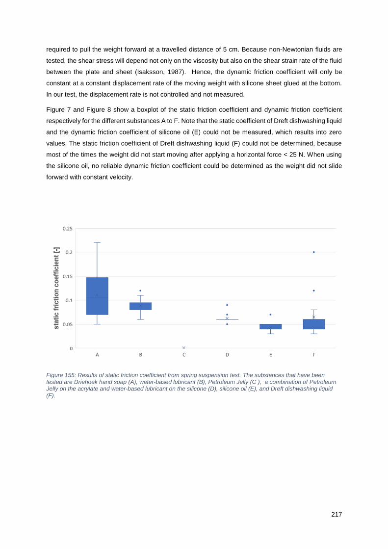
217
required to pull the weight forward at a travelled distance of 5 cm. Because non-Newtonian fluids are
tested, the shear stress will depend not only on the viscosity but also on the shear strain rate of the fluid
between the plate and sheet (Isaksson, 1987). Hence, the dynamic friction coefficient will only be
constant at a constant displacement rate of the moving weight with silicone sheet glued at the bottom.
In our test, the displacement rate is not controlled and not measured.
Figure 7 and Figure 8 show a boxplot of the static friction coefficient and dynamic friction coefficient
respectively for the different substances A to F. Note that the static coefficient of Dreft dishwashing liquid
and the dynamic friction coefficient of silicone oil (E) could not be measured, which results into zero
values. The static friction coefficient of Dreft dishwashing liquid (F) could not be determined, because
most of the times the weight did not start moving after applying a horizontal force < 25 N. When using
the silicone oil, no reliable dynamic friction coefficient could be determined as the weight did not slide
forward with constant velocity.
Figure 155: Results of static friction coefficient from spring suspension test. The substances that have been tested are Driehoek hand soap (A), water-based lubricant (B), Petroleum Jelly (C ), a combination of Petroleum Jelly on the acrylate and water-based lubricant on the silicone (D), silicone oil (E), and Dreft dishwashing liquid (F).

218
Figure 156: Results of dynamic friction coefficient from spring suspension. The substances that have been tested are Driehoek hand soap (A), water-based lubricant (B), Petroleum Jelly (C ), a combination of Petroleum Jelly on the acrylate and water-based lubricant on the silicone (D), silicone oil (E), and Dreft dishwashing liquid (F).

219
Appendix A.2: Pull-up test
Bathurst and Benjamin (1987) studied the influence of the sidewall friction on the vertical soil stresses
by surcharge loading for a large-scale unreinforced test in the paper ‘Preliminary Assessment of
Sidewall Friction on Large-Scale Wall Models in the RMC Test Facility’ (Bathurst and Benjamin, 1987).
He adopted Jewell’s relation (Jewell, 1987) in order to formulate a relation for the total sidewall force as
a function of depth, geometry of the test box, the horizontal earth pressure coefficient and the friction
angle between the sidewalls and sand. Here, the sidewall force is the vertical force which is transferred
to the sidewalls.
Bathurst and Benjamin (1987) divided the total sidewall force in two components, namely the sidewall
force due to (1) the self-weight of the soil and (2) the uniform external vertical load.
The unit sidewall friction is defined as:
𝑓𝑠𝑤 = 𝐾𝑠𝑤𝛾𝑧𝑡𝑎𝑛𝛿(𝐴2.1)
Accordingly, the sidewall force 𝑋𝑠𝑤 [kN] of one sidewall at depth z due to the self-weight of the soil can
be described by equation A2.2:
𝑋𝑠𝑤 =1
2𝐾𝑠𝑤𝛾𝑧
2𝐿𝑡𝑎𝑛(𝛿)(𝐴2.2)
𝐾𝑠𝑤 = the horizontal earth pressure coefficient at the sidewalls [kPa],
𝛾 = the unit weight of the soil [kN/m3],
𝑧 = the depth with respect to the top of the soil column [m],
L = length of the sidewalls [m]
𝛿 = the friction angle between the sidewalls and the sand [°]
The reduced vertical stress caused by surcharge loading is defined as follows:
𝑞(𝑧) = 𝑞0𝑒−2𝑧𝐾𝑠𝑤 tan(𝛿)
𝑊 (𝐴2.3)
𝑞0 = surcharge pressure [kPa],
𝑊 = width of the soil column [m].
The total surcharge force transferred to the sidewalls at depth z can be described by equation A2.4:
𝑋𝑞 = 𝑞0𝑊𝐿 (1 − 𝑒−2𝑧𝐾𝑠𝑤 tan(𝛿)
𝑊 )(𝐴2.4)

220
The relations proposed by Bathurst and Benjamin (1987) are used to derive the interface friction angle
between the sand and sidewall, 𝛿. In order to determine the sidewall force, Bathurst and Benjamin
(1987) measured the vertical earth pressures with pressure cells at different depths in a soil block of a
length and height of 6 m and 3 m respectively. The soil behind the wall was surcharged to 22 kPa, while
the wall was restrained vertically and horizontally at the toe (Bathurst and Benjamin, 1987). Since
pressure cells did not proof to be reliable at the low range of soil pressures in our test set-up. Another
test-set up, named the ´pull-up test´, was devised to measure the total sidewall force. The test set-up is
depicted in Figure 157.
Figure 157: Photo of test set-up
The concept of the pull-up test is to determine the vertical force transferred to the sidewalls by measuring
the difference between the force required to pull up the test box only and to pull up the test box prepared
with sand in combination with or without an additional known surcharge. Test facilities enable to measure
the total weight of the test box by means of an overhead crane, which is connected to the test box and
lifts it up vertically. By incorporating a load cell within the connection of the overhead crane and test box,
the required force to lift the test box is measured. A duplicate test box, but with an open bottom, is filled
with sand. The preparation procedure of densifying the sand is identical to the small-scale experiment
with relative densities in the same range of 70% ± 12%. Both sidewalls and the front-and back wall of
the test box were lubricated and covered with a thin silicone sheet in accordance with the preparation
procedure of the sidewalls in the small-scale experiment. Since Bathurst and Bejamin’s relations are
valid for surcharge loading, a surcharge load was created by placing 1 kg metal blocks across the entire
surface (Bathurst and Benjamin, 1987).

221
The vertical displacement was measured by a displacement sensor, which was attached to the test box.
Figure 159 shows at the vertical axis the percentage by which the vertical load in the soil is reduced due
to sidewall friction. A test was conducted with and without the lubricant and silicone sheet. The test
without lubricant and silicone sheet served as a check whether the lubricant and silicone sheet actually
reduced the friction between sand and sidewall.
Figure 158: Vertical displacement of silicone sheet against time during pull-up tests.
The measured tension force remains fairly constant for vertical displacements between 0.8 mm and 2
mm. Figure 158 shows the vertical displacement of the test box with respect to time. We observed that
the displacement increases linearly with time with a constant velocity for vertical displacements between
0.8 -2 mm for the test with silicone sheets on the sidewalls (red line). Accordingly, we assume that no
additional force is measured due to a nonzero acceleration. Furthermore, we assume that the frictional
forces between soil and sidewall are not altered after the < 2 mm vertical uplift.

222
Figure 159: Test results of pull-up test. On the vertical axis the percentage of total weight, which is transferred through the soil to the bottom of the test box. On the horizontal axis the displacement, which denotes the vertical
uplift of the test box.
From the test with silicone sheets on the sidewalls denoted by the red line in Figure 159, we conclude
that the total vertical force transferred to the soil is 52%. Hence 48% of the total weight is transferred to
the sidewalls. For a total soil weight of 20 kg, an additional load of 9.5 kg, the total sidewall frictional
force, 𝑋𝑚𝑒𝑎𝑠𝑢𝑟𝑒𝑑 , is 0.14 kN.
By implementing Bathurst and Benjamin’s relations, the total sidewall friction can be described by the
sum of the vertical force transferred to the sidewalls due to the self-weight of the soil, which induces
friction with the sidewalls as well as the front- and back wall (Bathurs and Benjamin, 1987).
𝑋𝑚𝑒𝑎𝑠𝑢𝑟𝑒𝑑(𝑧 = 𝐻) = 2𝑋𝑠𝑤(1)
+ 2𝑋𝑠𝑤(2)
+ 𝑋𝑞(1) + 𝑋𝑞(2)(𝐴2.5)
Here,
𝐻 = the height of the total soil column [m]
𝑋𝑚𝑒𝑎𝑠𝑢𝑟𝑒𝑑 = the total sidewall frictional force [kN]
𝑋𝑠𝑤(1)
= the vertical force transferred to the sidewalls due to friction between the self-weight of the soil
and the sidewall [kN]
𝑋𝑠𝑤(2)
= the vertical force transferred to the sidewalls due to friction between the self-weight of the soil
and the front wall or the back wall [kN]
𝑋𝑞(1) = the vertical force transferred to the sidewalls due to arching between the sidewalls [kN]
𝑋𝑞(2) = the vertical force transferred to the sidewalls due to arching between the front-and back wall
[kN]
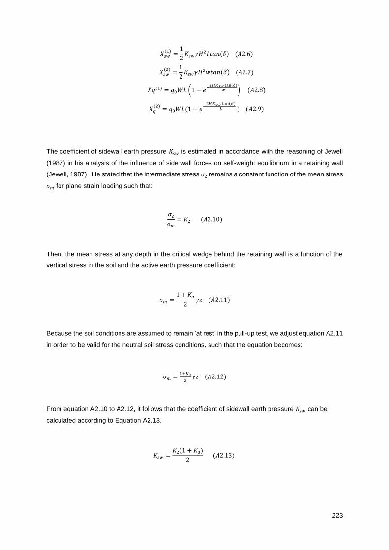
223
𝑋𝑠𝑤(1)
=1
2𝐾𝑠𝑤𝛾𝐻
2𝐿𝑡𝑎𝑛(𝛿)(𝐴2.6)
𝑋𝑠𝑤(2)
=1
2𝐾𝑠𝑤𝛾𝐻
2𝑤𝑡𝑎𝑛(𝛿)(𝐴2.7)
𝑋𝑞(1) = 𝑞0𝑊𝐿 (1 − 𝑒−2𝐻𝐾𝑠𝑤 tan(𝛿)
𝑤 )(𝐴2.8)
𝑋𝑞(2)
= 𝑞0𝑊𝐿(1 − 𝑒−2𝐻𝐾𝑠𝑤 tan(𝛿)
𝐿 )(𝐴2.9)
The coefficient of sidewall earth pressure 𝐾𝑠𝑤 is estimated in accordance with the reasoning of Jewell
(1987) in his analysis of the influence of side wall forces on self-weight equilibrium in a retaining wall
(Jewell, 1987). He stated that the intermediate stress 𝜎2 remains a constant function of the mean stress
𝜎𝑚 for plane strain loading such that:
𝜎2𝜎𝑚
= 𝐾2(𝐴2.10)
Then, the mean stress at any depth in the critical wedge behind the retaining wall is a function of the
vertical stress in the soil and the active earth pressure coefficient:
𝜎𝑚 =1 + 𝐾𝑎
2𝛾𝑧(𝐴2.11)
Because the soil conditions are assumed to remain ‘at rest’ in the pull-up test, we adjust equation A2.11
in order to be valid for the neutral soil stress conditions, such that the equation becomes:
𝜎𝑚 =1+𝐾0
2𝛾𝑧(𝐴2.12)
From equation A2.10 to A2.12, it follows that the coefficient of sidewall earth pressure 𝐾𝑠𝑤 can be
calculated according to Equation A2.13.
𝐾𝑠𝑤 =𝐾2(1 + 𝐾0)
2(𝐴2.13)

224
For 𝐾2, values of 0.65 to 0.75 for sand with a friction angle 𝜑 of 40° to 50° under plane strain-conditions
can be assumed (Jewell, 1987). For the preparation, the test box was gradually filled with sand and
simultaneously densified by means of tamping. Accordingly, it can be stated that the sand is slightly
overconsolidated. This results into a horizontal to vertical pressure ratio which will be higher than would
be according to Rankine’s theory (Rankine, 1857). The horizontal to vertical earth pressure coefficient
for neutral soil conditions, 𝐾0, is estimated to have an upper bound of 0.5 and the lower bound will be
described according to Rankine’s theory:
𝐾0 = 1 − sin(𝜑)(𝐴2.14)
Figure 160 shows the difference between the measured frictional force and analytical solution as a
function of the sidewall friction angle for the lower bound values of 𝐾0. For an internal friction angle of
45°, the analytical solution agrees with the measured value for an interface friction angle of 12.7°.
Considering the higher bound value of 0.5 for 𝐾0, the interface friction angle is determined at 11.0°.
Without the silicone sheet on the sidewalls, only 31% of the total vertical load was transferred to the soil.
For the lower bound and upper bound value of 𝐾0 and an internal friction angle of 45°, a value of 18.7°
and 16.2° was determined for the interface friction angle.
Figure 160: Derivation of interface friction angle estimated for the critical volume internal friction angle (𝜑𝑐𝑣) of 34°, internal friction angle at a confining pressure corresponding to the small-scale experiment conditions of 45°,
and internal friction angle at the peak friction angle (𝜑𝑝) of 50°.
225
Appendix A.3: Influence temperature and pressure differences on interface friction angle
The water content of the water-based lubricant is 85%. Glycerin (C3H803), which is an alcohol, and other
chemical additives are dissolved in the water. The water-based lubricant is assumed to behave in
accordance with the two synthetic solutions for which the viscosity was tested under different conditions
by Isaksson (1987). The tested synthetic solutions - containing different thickeners - had a water content
of 80 % and 88 %. Isaksson (1987) concluded that the synthetic solution with 80% water content
behaved more or less as a Newtonian fluid, while the synthetic solution with 88% water content behaved
as a non-Newtonian fluid. The reason was not assigned to the percentage of water content. However,
we can presume that the viscosity of the water-based lubricant will be sensitive to (1) the shear strain
rate, (2) temperature and (3) pressure. Accordingly, the interface friction angle between the sidewall and
sand will also have a dependency on the parameters above.
Because the static interface friction angle is larger than the dynamic interface friction angle, we neglect
the influence of the shear strain rate under the assumption that the shear strain rate does not influence
the static interface friction angle.
The findings of Isaksson (1987) for the two synthetic solutions is reckoned to be an indication of the
sensitivity of the viscosity to the temperature and pressure. For the maximum difference in pressure and
temperature between the spring-suspension test and the small-scale experiment, the viscosity can
reduce up to 0.3% due to a temperature increase as a consequence of the heat from the artificial light
sources. The pressure difference was of negligible influence on the viscosity. The reasoning behind
these statements are elucidated below.
According to Isaksson (1987), the shear stress 𝜏 of a non-Newtonian can be described as:
𝜏 = 𝐾�̇�(𝐴3.1)
Here, �̇� is the shear strain rate and 𝐾 is a power law coefficient. 𝐾 and �̇� are related with the viscosity 𝜇
according to the following formula:
𝜇 = 𝐾�̇�𝑛−1(𝐴3.2)
Here n is the power law index.
The power law coefficient 𝐾 consists of a temperature- and pressure dependent component,𝐾𝜃 and 𝐾𝑝.
𝐾(𝜃, 𝑝) = 𝐾𝜃(𝜃, 0)𝐾𝑝(0, 𝑝)(𝐴3.3)
The power law coefficient 𝐾 consists of a temperature- and pressure dependent component,𝐾𝜃 and 𝐾𝑝.

226
𝐾(𝜃, 𝑝) = 𝐾𝜃(𝜃, 0)𝐾𝑝(0, 𝑝)(𝐴3.4)
The temperature dependency is described by the power law coefficient 𝐾𝜃:
𝐾𝜃 = 𝑐1𝜃𝑐2(𝐴3.5)
The constants 𝑐1 and 𝑐2 were only given for the synthetic solution with 80 % water content. 𝑐1 and 𝑐2
were determined to be 0.1049 and -0.902. The temperature in the test hall during this test and the small-
scale experiment was similar. However, the artificial light sources radiated a lot of heat during the small-
scale experiment. Therefore, a maximum temperature increase from 18° C to 30° C is considered. This
temperature difference can lead to a reduction of 0.3% for 𝐾𝜃, and so for the viscosity.
The pressure dependency is described by the power law coefficient 𝐾𝑝:
𝐾𝑝 = 𝑒𝛼𝑝(𝐴3.6)
Here 𝛼 is the pressure coefficient in 𝑚2
𝑘𝑁 and p is the pressure in
𝑘𝑁
𝑚2.
The 5 kg weight with a diameter of 10 cm exerts a pressure of 6.4 kPa, while in the small-scale
experiment horizontal soil pressures range between approximately 0.5 and 20 kPa. Viscosity increases
as the pressure increases (Isaksson, 1987), which results into a higher interface friction angle between
the silicone sheet and acrylate plate.
For the synthetic solution with a water content of 88 % and 80%, the pressure coefficient 𝛼 was
determined to be 2.62 ∙ 10−12 𝑚2
𝑘𝑁 and 3.23 ∙ 10−12
𝑚2
𝑘𝑁. 𝐾𝑝 will be equal to 1 for the pressure range
considered in the small-scale experiment.

227
Appendix A.4: Stress-transducer test
Another test set-up is introduced to measure the loss of vertical stresses due to sidewall friction. A close-
up of the test set-up is schematized in Figure 161. Four metal plates having a size of 92 mm by 92 mm
are supported by rubber, which is in direct contact with the acrylate bottom of the test box. The metal
plates are overlain by a couple millimetres thick silicone layer which evens out the height difference
between the plates and the space in between. The space enclosed by the metal plates, rubber and
bottom of the test box, is filled with water and connected to a stand pipe. By making use of the very low
compressibility of water, it can be stated that the difference in water level in the stand pipe is a measure
of the pressure increase on top of the metal plate. Bending of the metal plates affects the water level in
the stand pipe. It would redistribute stresses and transfer them partly to the rubber side supports, leading
to less displacement of water within the enclosed space at the bottom of the box. In order to prevent
bending of the metal plates, the stiffness is increased by placing a second plate on top of the thin silicone
layer. This set-up was validated by filling the test-box completely with water and measuring the weight
of the water indirectly by the water level difference in the stand pipes. Knowing that no shear stress
exists between the sidewalls and stationary water, the friction between wall and water is zero. The linear
relation between the increasing weight of water in the test box and the increasing water level in the
stand pipes had proven the validity of the test set-up.
Figure 161: Schematization of the construction at the bottom of the test box for the measurement of the soil stress increase in the soil.

228
Appendix A.5: Extension test
The tensile stiffness of the silicone sheet is determined by means of three simple extension tests in
accordance with the test procedure described by Henkel and Gilbert (1952). They proposed a method
to estimate the effect of the rubber membrane on the measured triaxial compression strength of clay
samples. The extension test of the silicone sheets is depicted in Figure 162a.
Figure 162: Test set-up (a) and results (b) of extension test of silicone sheet.
Figure 162b shows the measured force per unit meter against the strain for the three tests. In order to
compare the resistance against extension of the silicone sheets with the resistance of the soil against
shearing, which is described by the shear modulus G, the tensile stiffness of the silicone sheet is
calculated as follows:
𝐸𝑇 =𝜎𝑇휀=
12𝐹
𝑡 ∙ 𝐵휀
(𝐴5.1)

229
Here,
t = the thickness of the silicone sheet [m],
B = the width of the silicone sheet [m],
F = the measured tensile force applied on the folded silicone sheet [N],
휀 = the strain of half the mean length of the silicone sheet L [-].
When ∆𝑢 is the measured length increment than the strain 휀 is calculated according to equation A5.2.
휀 =∆𝑢
𝐿(𝐴5.2)
Here, L [m] is the mean length of the silicone sheet, which is calculated according to equation A5.3.
𝐿 = 2(𝐷 − 𝑑 − 𝑡) + 𝜋𝑑(𝐴5.3)
Figure 163 depicts the geometrical parameters by which L is calculated.
Figure 163: Schematization of geometrical parameters in order to derive mean length of silicone sheet.

230
Appendix B
A similar definition and calculation procedure is applied for the derivation of the engineering linear soil
strains as was applied by White and Bolton (2001).
First, a displacement gradient matrix, L, is computed by means of shape functions:
𝑳 = [
𝜕𝑢
𝜕𝑋
𝜕𝑢
𝜕𝑌𝜕𝑣
𝜕𝑋
𝜕𝑣
𝜕𝑌
] (B.1)
Second, the displacement gradient matrix L is converted to the deformation gradient matrix F:
𝑭 = [
𝜕𝑥
𝜕𝑋
𝜕𝑥
𝜕𝑌𝜕𝑦
𝜕𝑋
𝜕𝑦
𝜕𝑌
] = 𝑳 + 𝑰 (B.2)
in which I is the identity matrix. Here, X and Y represent the horizontal and vertical coordinates of the
undeformed spatial coordinate system (i.e. the first photo of the set of test photos), while x and y
represent the horizontal and vertical coordinates of the deformed spatial coordinate system. Hence,
deformation gradient matrix F transforms a vector from undeformed coordinates (xi , yi) top deformed
coordinates (x’i , y’i).
(𝑥𝑖 ′
𝑦𝑖′ ) = 𝑭 (
𝑥𝑖𝑦𝑖) (B.3)
Third, by means of polar decomposition, the deformation gradient matrix F is decomposed into a strain
and rotational components. The strains are represented by the matrix U, which is the symmetric part
of F. U2 is commonly known as the Cauchy-Green strain matrix. The rotations are represented by the
matrix R, which is the skew-symmetric part of F.
𝑼 = (𝑭𝑇𝑭)1/2 (B.4)
𝑹 = 𝑭𝑼−1 (B.5)
Fourth, the Biot strain matrix (EBiot) is computed according to equation B.6.
𝐸𝐵𝑖𝑜𝑡 = 𝑼 − 𝑰 (B.6)
The Biot srain matrix (EBiot) includes the engineering linear strains: horizontal strains (휀𝑥𝑥), de vertical
strains (휀𝑦𝑦), and the shear strains (𝛾𝑥𝑦 = 휀𝑥𝑦 +휀𝑦𝑥).

231
휀𝑥𝑥 = 𝐸11𝐵𝑖𝑜𝑡 (B.7)
휀𝑦𝑦 = 𝐸22𝐵𝑖𝑜𝑡 (B.8)
𝛾𝑥𝑦 = 𝐸12𝐵𝑖𝑜𝑡 + 𝐸21
𝐵𝑖𝑜𝑡 (B.9)