analysis of oscillating systems purpose use the “improved euler method” – you learned this...

Analysis of Oscillating Systems

Purpose

• Use the “Improved Euler Method” – you learned this method of solving problems numerically in the homework.

• Compare measurements and numerical simulations of oscillating systems (spring-mass system).


The Euler Method Applied to Motion

• Uses the position , velocity, and acceleration of the system at one point in time to estimate the condition of that system at the next point in time.

• In general, the larger the time increments are, the more the estimation deviates from reality.


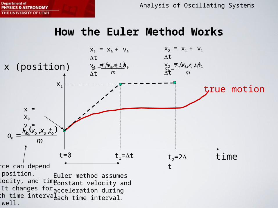
How the Euler Method Works

x (position)

timet=0

x = x0

v = v0

true motion

t1=Dt

x1 = x0 + v0 Dtv1 = v0 + a0 Dt

Euler method assumes constant velocity and acceleration during each time interval.

m

txvFa ooooo

,,

Force can dependon position, velocity, and time. It changes foreach time intervalas well.

m

txvFa 1111

1

,,

x1

x2 = x1 + v1 Dtv2 = v1 + a1 Dt

m

txvFa 2222

2

,,

t2=2Dt


Solution Easy in a Spreadsheet

time position velocity force acceleration

0

t1=Dt

t2= 2Dt

t3= 3Dt

etc.

xo voFo(xo, vo , to) ao=Fo/m

x1 = x0 + v0 Dt v1 = v0 + a0 Dt F1(x1, v1 , t1) a1=F1/m

x2 = x1 + v1 Dt

x3 = x2 + v2 Dt

v2 = v1 + a1 Dt

v3 = v2 + a2 Dt

F2(x2, v2 , t2)

F3(x3, v3 , t3)

a2=F2/m

a3=F3/m

initial conditions


How the Improved Euler Method Works

x (position)

timet=0

x = x0

v = v0

true motion

t1=Dt

x1 = x0 + v0.5 Dt

m

txvFa ooooo

,,

m

txvFa 115.01

1

,,

x1

t2=2Dt

v0.5 = v0 + a0 Dt/2

m

txvFa 225.12

2

,,

x2 = x1 + v1.5 Dt

v1.5 = v0.5 + a1 Dt

The improved method uses estimated velocity halfway betweenthe points in calculations Numerical simulation is closer to the true motion.


Improved Euler Method in a Spreadsheet

time position velocity force acceleration

0

t1=Dt

t2= 2Dt

etc.

xo vo

Fo(xo, vo , to) ao=Fo/m

x1 = x0 + v0.5 Dt F1(x1, v0.5 , t1) a1=F1/m

x2 = x1 + v1.5 Dt F2(x2, v1.5 , t2) a2=F2/m

initial conditions

t3= 3Dt x3 = x2 + v2.5 Dt F3(x3, v2.5 , t3) a3=F3/m

velocity athalfpoint

V0.5 = v0 + a0 Dt

V1.5 = v0.5 + a1 Dt

V2.5 = v1.5 + a2 Dt

V3.5 = v2.5 + a3 Dt


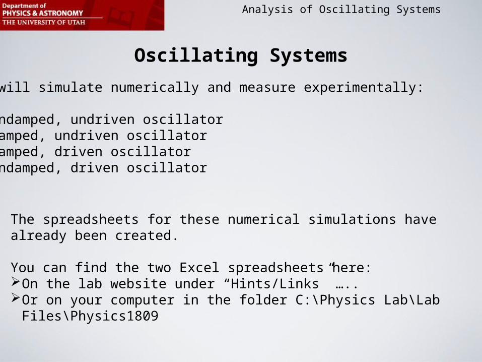
Oscillating Systems

You will simulate numerically and measure experimentally:

A. Undamped, undriven oscillatorB. Damped, undriven oscillatorC. Damped, driven oscillatorD. Undamped, driven oscillator

The spreadsheets for these numerical simulations have already been created.

You can find the two Excel spreadsheets here:On the lab website under “Hints/Links” …..Or on your computer in the folder C:\Physics Lab\Lab Files\Physics1809


Hooke’s Law

• Restoring force of a spring:

• Hanging a mass m at the end of the spring yields a change in the length of the spring (Dx).

Determine spring constant k:

xkF

x

mg

x

Fk

Dx


From theory:

.

Case A: Undamped, Undriven Oscillator

xkF Force acting on mass:

m

-x x

Rest position

+x

k

)cos()( tAtx

m

k


Hanging the Mass Vertically…

m

-x

x

Rest position with mass m

k

shiftxkF Rest position without mass m

mg

xshift

Total force on mass: kxmgxxkmgFF shiftspringtotal )(

Simply shift the coordinate system origin to the new equilibrium position and use Ftotal = - kx again (and ignore mg).

In the new equilibrium position: mgkxshift


Open spreadsheet:C:\Physics Lab\Lab Files\Physics 1809\Numerical_Analysis_Undriven_Oscillator.xlsx

.

Case A: Simulating the Undamped, Undriven Oscillator

Enter the mass and spring constant ofyour system. Thedamping constantb should be 0 forundamped motion.

Here you can also change the initialconditions (xo,vo)and the time increment of theEuler method.

More pages with graphs: Select here.


Here are theImprovedEuler Method

calculations,in case youwant to seehow they areimplementedin a spreadsheet.


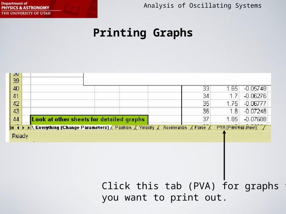
Printing Graphs

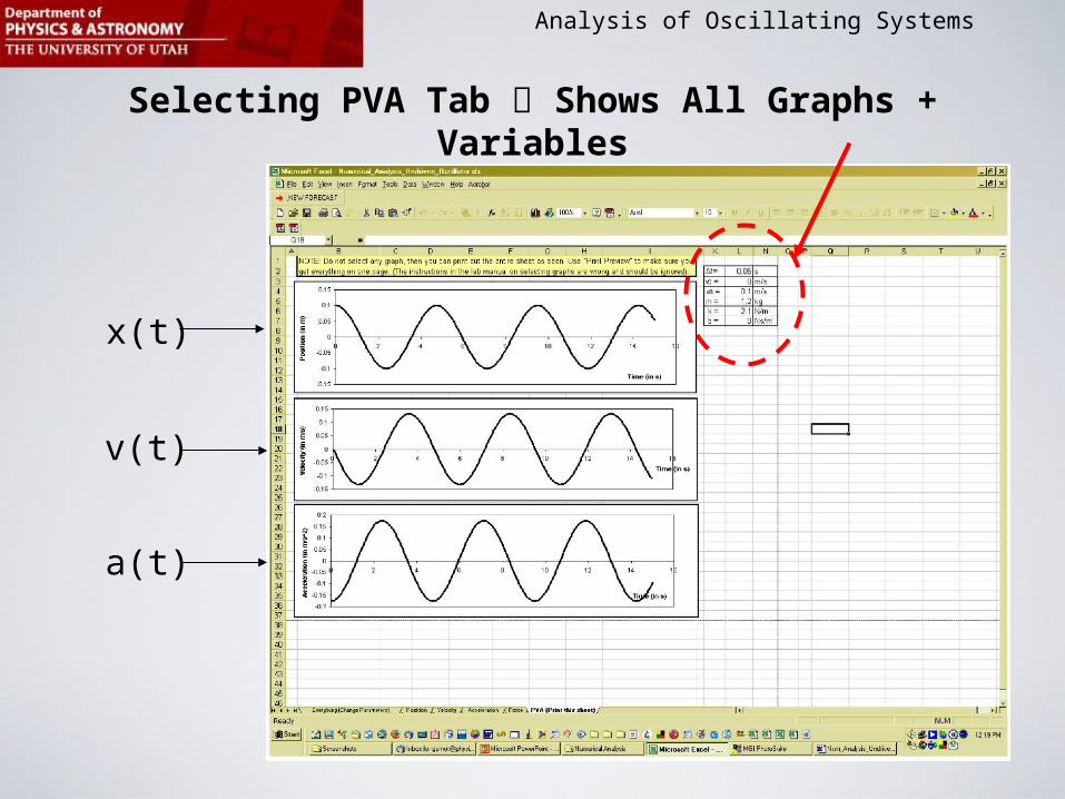
Click this tab (PVA) for graphs thatyou want to print out.


Selecting PVA Tab Shows All Graphs + Variables

x(t)

v(t)

a(t)


Case A: Experimentally Measuring the Undamped, Undriven Oscillator with Capstone

m

Mass oscillate around equilibrium point

Motion sensor measures x(t)

Please: Make sure that the mass does notcrash into or fall onto the motion sensor.The motion sensor is easily damaged.


Case B: Damped, Undriven Oscillator

m

Tape piece of thick paper/carton (e.g.,from a manila folder) at the bottom ofthe mass for damping.

Additional force:

vbxkFtotal

vbFdamp

Modify b (damping coefficient)in the spread sheet


Case C: Damped, Driven Oscillator

m

Additional driving force:

)sin( tDvbxkFtotal

)sin( tDFdrive

w

For the simulation spreadsheet use:

C:\Physics Lab\Lab Files\Physics 1809\Numerical_Analysis_Driven_Oscillator.xlsx


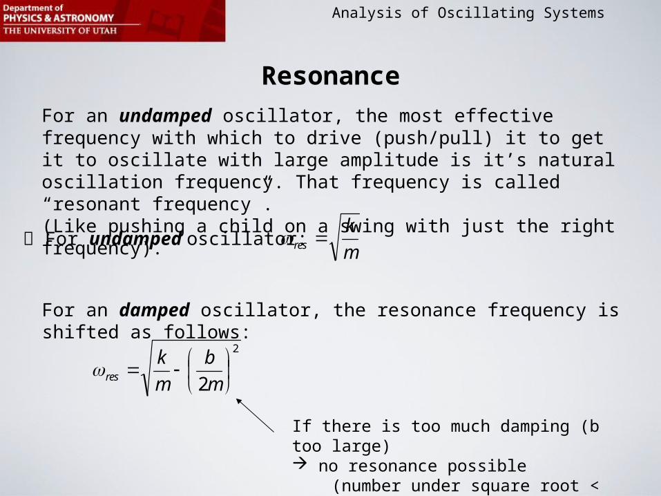
Resonance

For an undamped oscillator, the most effective frequency with which to drive (push/pull) it to get it to oscillate with large amplitude is it’s natural oscillation frequency. That frequency is called “resonant frequency”.(Like pushing a child on a swing with just the right frequency).

m

kres For undamped oscillator:

For an damped oscillator, the resonance frequency is shifted as follows:

2

2

m

b

m

kres

If there is too much damping (b too large) no resonance possible (number under square root < 0).


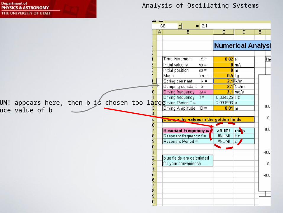
If #NUM! appears here, then b is chosen too large Reduce value of b


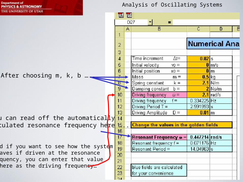
After choosing m, k, b …..

…you can read off the automatically calculated resonance frequency here …..

…and if you want to see how the systembehaves if driven at the resonancefrequency, you can enter that valueup here as the driving frequency…


Case C: Damped, Driven Oscillator - Experiment

Driver/Oscillator:powered by 750 Interface

amplitude adjustment


Amplitude Adjustment …

Amplitude: If amplitude istoo large, oscillator may notrotate (too much torque dueto weight).

Reduce amplitude if necessary


Weights

Use these specially made aluminum weights only !!(They have the proper weightneeded).


Running the Driver/Oscillator from Capstone

Record button will activatedriver and motion sensor (not in picture).

DC voltage determinesthe driving frequency.

DC voltage adjustable to fine tune driving frequency.


Improper Driver Frequency Beat Patter is Observed

Beat period:Here approx. 10s

Beat frequency=1/10s=.1 Hz

Our drivingFrequency is offby 0.1 Hz (eithertoo low or toohigh)

Change DCvoltage


How Much Adjustment in DC Voltage ???

Rule of thumb:A change of 1 Volt changes the driver frequency by 0.2Hz

For a beat frequency of 0.1Hz we need to change the DC voltage by

VoltVoltV 5.02.0

1.01

Before, we had: 4.0 Volts Try 3.5 Volts or 4.5 Volts(one will make beat frequency greater, the other will make it disappear)


Trying 4.5 Volt Works in Our Case…

Amplitude keeps growing, no beat pattern observed.


Case D: Undamped, Driven Oscillator

m

)sin( tDxkFtotal

w

For the simulation spreadsheet use again:C:\Physics Lab\Lab Files\Physics 1809\Numerical_Analysis_Driven_Oscillator.xlsx

Careful: Without damping the amplitudesat resonance can get HUGE. Don’t let themass slam into the motion sensor!!!!

No more cardboard to dampen motion


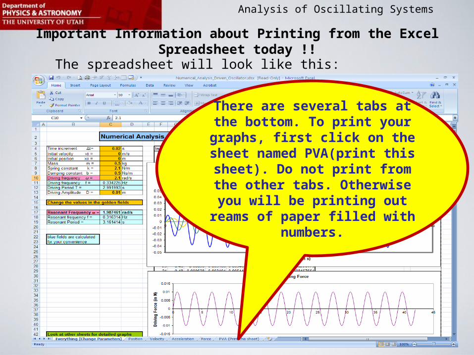
Important Information about Printing from the Excel Spreadsheet today !!

The spreadsheet will look like this:

There are several tabs at the bottom. To print your graphs, first click on the sheet named PVA(print this sheet). Do not

print from the other tabs. Otherwise you will be printing out reams of paper filled with

numbers.


Once you are at the PVA-tab of the spreadsheet it looks like this:

Make sure that ONLY the PVA tab is selected and use the “Print Preview” command to make sure you are only printing what you want to have printed.

Thank you for helping preserve resources!

analysis of oscillating systems purpose use the “improved euler method” – you learned this...

Documents

v0 a0 dt euler method

x0 v0 dtv1

v0 a0 dtv1

v0 a0 dtf1x1

x1 v1 dtv2

v1 a1 dtv3

v0 a0 dt2 x2

x1 v1 dtx3