analysis of opportunities to implement steam driven...

Analysis of opportunities to implement Steam driven fans in new formaldehyde plants Master’s Thesis within the Innovative and Sustainable Chemical Engineering programme

SYED AMIR ALI SHAH Department of Energy and Environment Division of Heat and Power Technology CHALMERS UNIVERSITY OF TECHNOLOGY Göteborg, Sweden 2012

MASTER’S THESIS

Analysis of opportunities to implement Steam driven fans in new formaldehyde plants

Master’s Thesis within the Innovative and Sustainable Chemical Engineering

SYED AMIR ALI SHAH

SUPERVISOR(S):

MATTEO MORANDIN

ANDREAS MAGNUSSON

EXAMINER

Prof. SIMON HARVEY

Department of Energy and Environment Division of Heat and Power Technology

CHALMERS UNIVERSITY OF TECHNOLOGY Göteborg, Sweden 2012

Analysis of opportunities to implement steam driven fans in new formaldehyde plants Master’s Thesis within the Innovative and Sustainable Chemical Engineering programme SYED AMIR ALI SHAH

© SYED AMIR ALI SHAH, 2012

Department of Energy and Environment Division of Heat and Power Technology Chalmers University of Technology SE-412 96 Göteborg Sweden Telephone: + 46 (0)31-772 1000 Chalmers Reproservice Göteborg, Sweden 2012

I

Analysis of opportunities to implement steam driven fans in new formaldehyde plants Master’s Thesis in the Innovative and Sustainable Chemical Engineering programme SYED AMIR ALI SHAH Department of Energy and Environment Division of Heat and Power Technology Chalmers University of Technology

ABSTRACT The purpose of this Master thesis (project) is to perform a conceptual design and an economic viability study of steam turbine system for production of power which can be used to partially or totally cover the power requirements of the recirculation blowers in a chemical process. In this project a process for production of 52500 ton/year of Formaldehyde 37 wt% with a consumption of 22300 ton/year of Methanol has been studied.

Based on a reactor using metal oxide catalyst, formaldehyde is produced by means of methanol catalytic oxidation. The formalin plant operates slightly above the atmospheric pressure. The speed of the recirculation blowers increases in order to overcome the pressure drop that occurs in reactor when the catalyst is getting old. Due to degradation of the catalyst the pressure drop increases therefore at some point the pressure drop reach a level where the catalyst must be replaced with new catalyst.

The oxidation is highly exothermic. In order to promote the high conversion of methanol the reaction is kept at given temperatures by means of oil cooling HTF. Oil cooling is achieved by generating steam from condensate. In the standard process, steam is produced at medium pressure.

Process heat integration analysis is carried out to find the maximum thermodynamic potential of power generation. The maximum steam superheating temperature and steam mass flow rate are estimated by means of simple Pinch Analysis calculations. By comparing the power production potential and the power consumption over an average year, different possible design solutions for turbo machinery arrangement (Single Shaft or Double shaft system) are considered and two main design options from vendors are discussed. The different designs are compared considering two main profitability criteria: payback time and net present value. In particular, the total investment cost for single shaft design is around 334’000 €. The revenues in terms of electricity savings is around 146’000 €/year. The payback time for this system is 3 years. The total investment cost for double shaft design is around 200’000 € and the revenues in terms of electricity savings is around 94’000 €/year. The payback time is also 3 years for this design. While the pay-back time does not help to identify the best system option, a discounted cash flow analysis shows that the net present value at the end of 10 year is higher for the single shaft system compared to the double shaft system case.

III

Contents ABSTRACT I

CONTENTS III

ACKNOWLEDGEMENT V

NOTATIONS VII

1 BACKGROUND 1

1.1 Introduction 1

1.2 Objective of thesis 2

1.3 Thesis outline 3

2 DETAILED DESCRIPTION OF THE STANDARD FORMALDEHYDE PRODUCTION PLANT (REFERENCE YEAR 2012) 5

2.1 Production of formaldehyde 5

2.2 Definition of the reference plant operation 8

2.3 Main thermal loads of the plant and thermal utility requirements 8

2.4 Main electricity consumption units 9 2.4.1 Pressurization Blowers 9 2.4.2 Recirculation Blowers 9 2.4.3 Electric heater with ECS reactor 9 2.4.4 Electric heater with HTF system 9 2.4.5 Pumps 9 2.4.6 Total electricity consumption of the plant 9

3 CHARACTERIZATION OF THE REACTOR PRESSURE DROPS AND OF THE BLOWER POWER REQUIREMENT 11

3.1 Pressure drop profile in the reactor 11

3.2 Estimation of the blower power profile and total yearly electricity consumption 12

4 ESTIMATION OF POWER PRODUCTION POTENTIALS 15

4.1 From thermal loads to aggregate heat load/temperature profile 15 4.1.1 What is Pinch Analysis? 15 4.1.2 Grand Composite Curve of the formaldehyde plant 16 4.1.3 Operating parameters of a heat recovery steam turbine cycle for maximum power generation 17 4.1.4 Theoretical electricity savings opportunities 25

5 CONCEPTUAL DESIGN FOR PRACTICAL WORK RECOVERY IN THE FORMALDEHYDE PLANT 27

5.1 Method for preliminary selection of turbo machinery 27

5.2 Estimation of practical potential of electricity generation 30

IV

5.2.1 Super heater 30 5.2.2 Concise overview of steam turbines 31 5.2.3 Preliminary estimates of steam turbine power 31

5.3 Screening of the concepts 33 5.3.1 Steam driven blowers 33 5.3.2 Separate steam turbine set 34

6 SOLUTION FROM VENDORS 37

6.1 Vendor A (Double Shaft Configuration) 38 6.1.1 Estimation of the blower nominal performances based on the quoted turbo-machinery speed 38 6.1.2 Estimation of the blower power requirement profile based on the quoted characteristic curves 39 6.1.3 Preliminary estimation of the turbine performance based on the quoted nominal speed 41 6.1.4 Estimation of the turbine power based on the obtained blower shaft speed 43 6.1.5 Electricity savings 45 6.1.6 Profitability analysis 47

6.2 Vendor B (Single Shaft Configuration) 50 6.2.1 Estimation of the blower nominal performances based on the quoted turbo-machinery speed 51 6.2.2 Estimation of the blower power requirement profile based on the quoted characteristic curves. 51 6.2.3 Preliminary estimation of the turbine performance based on the quoted nominal speed 53 6.2.4 Estimation of the turbine power based on the obtained blower shaft speed 55 6.2.5 Electricity savings 56 6.2.6 Profitability analysis 58

7 SUMMARY OF RESULTS AND CONCLUSION 61

7.1 Electricity savings and profitability 61

7.2 Conclusion 62

8 REFERENCES 63

9 APPENDIX 65

9.1 Estimation of Blower Power 65

9.2 Estimated power from the steam turbine 67

9.3 Blower and Steam Turbine Specifications 68

9.4 Consequence on available heat at the turbine outlet (Double shaft configuration) 69

9.5 Consequences on available heat at the turbine outlet (Single shaft configuration) 70

9.6 Economic Factors 70

V

Acknowledgement I would like to thank Professor Simon Harvey for letting me work on this project and guiding me nicely throughout the project. It was a great opportunity for me. I learned precious knowledge while working with extremely talented team. I would also thank Andreas Magnusson for his direction, assistance, and guidance. Special thanks to Matteo Morandin, whose recommendations and suggestions have been invaluable for this project. I also wish to thank Ola Erlandsson, who have helped me lot. His company was always nice and beneficial. Finally, words alone cannot express the thanks I owe to, my parents. Their prayers made this all happened.

Thank you all!

VII

Notations S Entropy [J/kg K]

Q Heat [J]

T Temperature [C]

P Pressure [bar]

h Enthalpy [J/kg]

Cp Specific heat capacity at constant pressure [J/kg K]

V Relative speed [m/s]

m Mass flow [kg/s]

ns Specific speed [m/s]

l Length [m]

ds Specific diameter [m]

A Area [m2]

n Speed [rpm]

ΔH Heat of Vaporization [J/kg]

T Time

HTF Heat transfer fluid

ECS Emission control system

Greek η Efficiency

ηis Isentropic Efficiency

ω Angular speed [rad/s]

ρ Density [kg/m3]

Suffixes t Turbine

c Compressor

1

1 BACKGROUND The present work focuses on potential improvements of the energy performance of the Formaldehyde process, a well consolidated process concept for the production of Formalin, a water solution of Formaldehyde, which is used as a key material for products such as coating, paint and plastics (Hagman & Walhelm, 2005).

Cash flows for industrial plants are normally dependent on the fluctuation of energy market prices due to fuel purchases, purchase or sales of electricity and district heating deliveries. Thus it is hard to evaluate the long term outcome of an economic investment in the plant’s energy system. In the analysis of energy efficiency investments it is important to consider the uncertainties of the future energy market conditions. For plants located in countries in which prices of electricity are high, electricity production is often a robust investment (Svensson, 2008).

1.1 Introduction Chemical processes are significant energy consumers mainly due to their large heating demands. As these demands are primarily met through the use of steam, they provide a good potential for efficient cogeneration of power through the use of steam turbines. Efficient cogeneration calls upon better designs of utility systems, as well as more efficient operation of the existing equipment. Steam systems deliver the required heat, mechanical power, and electricity demands to typical chemical plants. Steam demands result from the heat required by process steam heaters as well as steam required as reactant by the reaction system. Several process devices require also electricity, such as electrical heaters or for motors. In order to avoid the costs of electrical drivers and their conversion losses, some of these process devices (e.g. compressors) can be coupled to steam turbines for direct exchange of mechanical power.

In the process under investigation in this thesis, steam is raised as a result of cooling of a high temperature exothermic reaction. There are different ways in which we can use steam internally in order to produce electricity with a steam turbine and use its power for running process equipments.

After talking with the engineers at the company initiating this work, it was decided to explore the option of using the power production from steam turbine to minimize the electricity required by the recirculation blowers.

Different configurations of steam driven recirculation blowers were investigated in this project. In particular, as steam can also be used for heating in nearby processes (i.e. sold), two types of steam turbines can be considered. If steam also is required for process heating, a back-pressure steam turbine can be used whereas if the steam is to be exclusively used for electricity production, a condensing steam turbine can be implemented (Cardu, 1993). A condensing steam turbine allows more power production and can be of interest if the largest part of the process power requirement has to be covered (e.g. in order to minimize the purchase of expensive grid electricity). However, for this configuration, a condenser is required after the turbine which can lead to high investment costs.

2

Here follows the brief description of the formalin process. Fresh air is pressurized, to overcome the pressure losses in the formalin process loop in the so called re-circulation blowers. These re-circulation blowers are the main energy consumers in the formalin process. Methanol is pressurized and the mixture of methanol-air is led into the formaldehyde reactor where a catalyst triggers the oxidation. Because that oxidation is exothermic, a large amount of heat is generated in this reactor. The reactor is cooled using pressurized oil as the cooling medium. The vaporized oil is then condensed in a condenser that produces medium pressure steam. After the formaldehyde reactor, the gas is sent to absorption tower where the formaldehyde is absorbed in water. After the absorption tower, it enters into the ECS (Emission Control System) to be cleaned from the rest of hydrocarbon, carbon monoxide, dimethyl ether and methanol it contains. This is done by oxidation in the ECS reactor. The exothermic reaction generates heat, and small amount of medium pressure steam is produced in the ECS steam generator. After the ECS these gases lead to the stack and out to the atmosphere. A more detailed description of the process is presented in the next chapter.

Since in the reference plant design there are only two heat exchangers (one between main reactor and water evaporation, one between ECS reactor and water preheating) it means that the theoretical electricity savings opportunities calculated here can be achieved only through major plant re-design which is beyond the scope of the present study.

There are different ways in which the steam turbine and the electrical motors can be coupled with the pressurization blower system. This is not only a question of investment and electricity savings related to the chemical process design point (nominal conditions) but some technological issues related to plant operations should also be considered. The plant start-up for instance requires installation of an electrical motor to be used to overcome the catalyst pressure drops, as steam starts to be available only after the exothermic catalytic reaction has started. Only at that point the circulation blowers can be switched from the electrical motor to be driven with a steam turbine.

With time, the catalyst inside the reactor degrades, so more pressure drop occurs for a given gas flow and more power is therefore required to overcome such pressure drops (Formox, 2006). In such case therefore, the contribution of the electrical motor can vary during the plant operation.

The plant behaviour during the year must be therefore taken into account in order to discern the best design among all the theoretical possible arrangements.

1.2 Objective of thesis The objective of this master thesis is to investigate possible new design options that reduce the need to purchase the process electricity from the grid.

In particular, this work focuses on the investigation of steam expansion to recover the work production potential of the medium pressure steam raised by cooling the exothermic reactor which is today used only for heating purposes and often bled to much lower pressures. This involves understanding thermodynamic and technological limitations for maximum steam production, steam network parameters (maximum

3

pressure and temperature, steam turbine backpressure), and the relative impact on process profitability of different arrangements of turbo-machinery.

The study is conducted as a conceptual design of a new re-circulation blower section of the chemical plant concept under investigation and not as a retrofit of already existing plant.

The profitability of the new steam driven re-circulation blower options is assessed by comparing associated cash flows with that of the electricity driven re-circulation blowers of the reference base case standard plant.

1.3 Thesis outline The first chapter provides an introduction to the work carried out in this project by giving a background and also presenting the aims and objectives for the thesis project. The next chapter presents the detailed description of the plant including process description of the formaldehyde production, main thermal loads of the plant and major electricity consumption units.

Chapter 3 presents the characterization of the reactor pressure drop and of the blower power requirement.

Chapter 4 provides an overview of the maximum thermodynamic potential of power generation.

Chapter 5 discusses the conceptual design of steam driven re-circulation blowers for practical work recovery in the formaldehyde plant.

Chapter 6 gives the economic evaluations of different configurations of turbo machinery as indicated by vendors that were contacted during this study.

Results and Conclusions are presented in Chapter 7.

5

2 DETAILED DESCRIPTION OF THE STANDARD FORMALDEHYDE PRODUCTION PLANT (Reference Year 2012)

2.1 Production of formaldehyde Formaldehyde is produced by partial catalytic oxidation of methanol in air. The reaction takes place on a metallic oxide catalyst, using a fixed tube bed vapour phase oxidation reactor, according to the following stoichiometry: CH3OH + 1/2 02 → CH20 + H20 (2.1) A low ratio of methanol to air is used to maintain the desired oxidation atmosphere. The methanol content in air is maintained between about 4 and 10 vol%. Such a high methanol content can be used because part of the gas from the absorber is recycled, which decreases the oxygen concentration sufficiently to avoid explosive mixtures (Formox, 2006).

As shown in the main process flow diagram in Figure 2.1, the heat of reaction is removed from the main reactor by boiling a liquid, hereafter referred to as heat transfer fluid (HTF). The process gives a high yield of formaldehyde on a single passage, and also very high methanol conversion. The actual formaldehyde yield is in the range of 91-94 % of the theoretical. The remaining methanol is accounted by un-reacted methanol, carbon monoxide, dimethyl ether and a negligible amount of formic acid. The fresh air is supplied by a pressurization blower and, after mixing with recirculation gas, pushed through the process by two recirculation blowers. Methanol is supplied to the plant by a pump. The methanol is vaporized and the gas mixture is heated when the process gas-methanol mixture is passed through the methanol vaporizer.

The oxidation of the methanol takes place on the catalyst in the tubes of the main reactor. The tubes are loaded with the metallic oxide catalyst to a specific depth. The bottom and the top sections of the tubes are filled with small inert rings to improve heat transfer. The shell side of reactor is filled with HTF to remove part of the heat of reaction. The gas mixture is preheated by boiling the HTF in the top of the tubes. As the gas reaches the heated catalyst, the reaction starts and the temperature rise rapidly to a maximum. When the main part of the methanol has reacted, the temperature drops rapidly again and approaches the temperature of the boiling HTF when the gas leaves the reactor tubes. (Formox, 2006).

The circulation of HTF to the reactor shell and into HTF condenser is carried out by thermo siphon circulation. The vapours of HTF are condensed in a shell-and-tube heat exchanger. The condensation heat is recovered to produce medium pressure steam. The HTF condenser is therefore also operated as a steam boiler and it gives excess steam as compared to the steam production from ECS (Emission Control System) steam generator. During start-up, before the heat of reaction has achieved sufficient thermo siphon circulation, the HTF is circulated by a pump and heated by an electrical heater. During the conversion of methanol into formaldehyde, some side reactions occur, which are:

6

Side reactions: CH3OH + 02→ CO + 2 H20 (2.2) (Carbon monoxide) CH3OH + 02→ HCOOH + H20 (2.3)

(Formic Acid)

2CH3OH→ CH3OCH3 + H20 (2.4)

(Dimethyl ether)

From the bottom of main reactor the reacted gases pass through the methanol vaporizer. These gases are cooled to a temperature to about 120°C in the methanol vaporizer, depending upon the flow of methanol. From the methanol vaporizer these gases flow into the Absorber. The reactive formaldehyde is absorbed in water, in the absorption tower. The gas is passing upward through water/formalin over different packing materials. These packing maximize the contact area between water and formaldehyde gas. So liquid is cooled in several steps and sometimes caustic soda is added from the top. All these measures will increase the efficiency of the absorption tower. The formalin solution is finally stored in a storage tank (Formox, 2006).

From the top of the absorption tower the gas flow is split between ECS (Emission Control System) and recirculation blowers. To the ECS, the amount of gas is controlled by an oxygen control valve. This valve controls the proportions of recycle gas and fresh air in such a way that the oxygen concentration of the process gas is kept constant after the recirculation blowers. Approximately 1/3 of the gas after the control valve enters into the ECS system, where hydrocarbons, carbon monoxide, dimethyl ether, formaldehyde and methanol are converted into carbon dioxide and water through catalytic combustion. The oxidation of the gas is done in an ECS reactor over a bed of noble-metal catalyst.

The following oxidation reactions take place: CO + 1/2 02 →CO2 (2.5)

CH3OCH3 + 3 02 →2CO2 +3H20 (2.6)

CH20 + 02 →CO2 + H20 (2.7)

CH3OH + 3/2 02→ CO2 + 2H20 (2.8)

As the catalytic combustion is highly exothermic it generates heat which can be used for internal heat recovery and for steam production. After passing from ECS reactor and steam generator, the high temperature gas flow enters the other side of the ECS pre-heater. During start-up, the ECS reactor is heated by an electrical heater before the catalyst bed has ignited. Before the gas enters into the ECS reactor from ECS pre-heater, this ECS pre-heater preheats the ECS gas flow to the ECS reactors catalyst ignition temperature. After passing through the ECS pre-heater this gas is lead to the stack and out to the atmosphere (Formox, 2006).

7

1

2

3

4

5

6

8

9

10

11

12

METHANOL FEED

FRESH AIR

Pressuriza-tion Blower

Recircula-tion Blower

Recircula-tion Blower

Methanol Prevap-orizer

Methanol VaporizerMain

Reactor

HTF Cond.

Cooler

Product Cooler

Pump

Pump

Absorber

PS1

PS2

PS3

Pump

Cooler

ECS Preheater

ECS (Emission

Control System) Reactor

ECS Steam

GeneratorFW

COOLING WATER FEED

COOLING WATER RETURN

FORMALDEHYDE

PROCESS WATER

TO STACK

Saturated Steam

FW

13

Saturated Steam

PumpFW Tank

From City Outer battery

limit

1411

15

16

1718

2019

21

22

23

V-5

7

V-4

V-1

E-1

V-2

Cooler

V-6

To other plant

Steam NetTo the FW

tank

Pump

Cont-rol valve

Figure 2.1 Process flow diagram of the current “standard” design (Formox, 2006).

8

2.2 Definition of the reference plant operation The current “reference” formaldehyde plant evaluated allows for a maximum capacity of 52500 ton/year of Formaldehyde with a consumption of 22300 ton/year of Methanol. For evaluation the plant is assumed to operate for 350 days/ year at 100% capacity. The production capacity of the plant load at 100% is 150 ton/day. Due to degradation of the catalyst the pressure drop increases inside the reactor therefore at some point the catalyst must be replaced with a new catalyst.

2.3 Main thermal loads of the plant and thermal utility requirements

The main thermal loads of the plants are the Main reactor and the ECS reactor as shown in Table 2.1. Heat is generated in the main reactor due to the exothermic reaction. The HTF pump is used to circulate the HTF into the reactor and the HTF condensers, at the start-up the HTF heater is used to heat the HTF to the correct start temperature in the reactors. The HTF is used on the shell side of reactor in order to recover heat which causes the HTF to boil in the reactor. The HTF vapours leave the reactor shell and move into the HTF condenser. In the HTF condenser the HTF vapours condenses. The condensed HTF is collected in the separator. The level in the separator is indicated by the level indicator. The steam is generated (by flowing water counter-currently) in the HTF condenser as the feed water evaporates due to heat of condensation of the HTF.

For start-up purposes (only 6 hours), the ECS reactor is equipped with an electric heater. The purpose of the electric heater is to ignite the bed, after which there is no more need of electric heater since the process is self-sufficient due to the exothermic reactions. The exhaust gas from the absorber passes into the catalytic chamber where it is oxidized over a bed of noble metal catalyst. The temperature increases due to the exothermic reaction. The hot gases leaving the catalyst bed then passes through the ECS steam generator which is also cooled by feed water. Only a minor part of the total process steam is generated in the ECS steam generator by cooling the hot stack gas leaving the catalyst bed (Formox, 2006).

Table 2.1 Summary about thermal loads of the plants and steam available for export in the standard plant

Main thermal loads of the plant

Q [kW] Steam available for export in the standard plant

[kg/hr]

Main reactor 2268 3390

ECS reactor 795 618

9

2.4 Main electricity consumption units The major electricity consumption units in the formaldehyde plants are described below (Formox, 2006).

2.4.1 Pressurization Blowers The pressurization blower is of Roots type. To maintain a constant pressure in the system, a pressure controller controls the inlet air by adjusting the blower speed with a frequency convertor.

2.4.2 Recirculation Blowers The recirculation blowers, which supply the air for the oxidation process, are of centrifugal type. They are connected in series. The flow controller controls the process gas flow by adjusting the blower speed via frequency convertor. Immediately after the blowers, a sample of process gas is continuously withdrawn and passed through two oxygen analyzers. The measured process gas flow is used for calculating the methanol volume % in the process gas.

2.4.3 Electric heater with ECS reactor For start-up purposes, the ECS reactor is equipped with an electric heater. The heater is switched on and off from the distributed control system (DCS).

2.4.4 Electric heater with HTF system The HTF heater is used to heat the HTF to the correct start temperature in the reactors. It is operated only at start-up to regulate the reactor temperature.

2.4.5 Pumps Pumps are used to move fluids into the different units like HTF condenser, absorber, and a product cooler.

2.4.6 Total electricity consumption of the plant The total yearly average electricity consumption by (pressurization, recirculation blowers, pumps and heaters) is 3’400 MWh. The electricity consumed by the recirculation blowers is 2’180 MWh.

Table 2.2 Summary related to electricity consumption of the plants

Main electricity consumption units of the plant

Electricity consumption [MWh]

Re-circulation blowers 2’180

Pressurization blower 750

Pumps 350

Electric heaters 100

11

3 CHARACTERIZATION OF THE REACTOR PRESSURE DROPS AND OF THE BLOWER POWER REQUIREMENT

This chapter focuses on the power requirements of the recirculation blowers, the process units which have been identified as the potential location for new energy savings measures.

The power requirement of the recirculation blowers gets higher during the process operation due to degradation of the catalyst.

No clear data about pressure drops in the reactor are available except for the minimum and maximum values.

In this chapter the method for estimating how the pressure drops vary in the reactor when the catalyst is getting old is described and some conclusions are drawn on the consequent blower power requirement profile.

3.1 Pressure drop profile in the reactor In order to estimate the pressure drop profile in the reactor, the length of normal cycle is 240 days/year. When the catalyst is fresh the pressure drop over the process is 0.47 bar, and when the catalyst is getting old the pressure drop over the process is 0.82 bar. When the catalyst is completely degraded then we need to replace the old catalyst with a fresh catalyst in order to increase the catalytic oxidation reaction in the main reactor. By considering constant production of 150 ton/day a polynomial model of 2nd degree was selected to estimate how pressure drop varies with time in the main reactor over the typical load (240 days/year). The polynomial model of the pressure drop profile is then used to estimate the power profiles of the blowers and eventually to get the total electricity consumption over the typical load. The general expression for the 2nd degree polynomial is

𝑦 = ax2 + bx + c (3.1) Where “y” is the Δp in bar, “x” is the time in days and “a, b, c” are the constants. We have a boundary limit for pressure drop in the process, At x=0, meaning when t=0 days, then y=c=Δp=0.47 from the above eq. (3.1) x= 240, means when t= 240 days, then y=Δp=0.82 y=0.82=a.(240)2+b.(240)+0.47 (3.2) The derivative of eqt (3.1) is,

12

𝑑𝑦𝑑𝑥

= 2𝑎𝑥 + 𝑏 (3.3) The derivative of equation (3.1) is 0 at y=0, because the slope of line is tangent, so b=0 then after simplification of eq. (3.2), we get Δp as a function of time. 0.82-0.47=a.57600 and a=6.076.E-6

𝛥𝑃(𝑡) = 6.076E − 6. (t)2 + 0.47 (3.4) Eqt (3.4) returns the pressure drop profile [bar] in the reactor over time [days]. The generated profile is shown in the figure below.

Figure 3.1 Pressure drop profile in the reactor

3.2 Estimation of the blower power profile and total yearly electricity consumption

In the standard design, the two recirculation blowers are connected in series (i.e. two stages, two different shafts) and they are driven by two electrical motors as shown in Figure 3.2.

13

HCHO Proces

s

M

M

Fresh Air

Pressurization Blower

Recirculation Blowers

Prod

M

Figure 3.2 Combination of re-circulation blowers in the standard design

To estimate the blowers’ power profiles and the total yearly electricity requirement according to the pressure drop profile above, some calculations are required to estimate the blower performance.

According to the given volumetric flow rate, available as a process data, the shaft power of the blower is calculated from the procedure described in Handbook of Modern Fan Technology (Fans, 1997). The other required data for estimation of blower power is the mass and energy balances. The procedure for calculating the blower power is described in Appendix. Table 3.1 Electricity consumption in the recirculation blowers

Cases 100% (150 ton/day)

Pressurized + Fresh Catalyst (0,3-0,77 barg) 219 kW Pressurized + Old Catalyst (0,3-1,12 barg) 351 kW We use the same 2nd degree polynomial model for estimation of outlet pressure P2 after the 2nd stage of recirculation blower.

𝑃2(𝑡) = 6.076E − 6. (t)2 + 0.47 (3.5) Eqt (3.5) returns the outlet pressure P2 [bar] over time [days].

The procedure described in Appendix 9.1 from eqt. (9.1) to eqt. (9.19) is used to estimate the total fan shaft power requirement per load. The blower power profile over a typical load is shown in Figure 3.3.

14

Figure 3.3 Variation of blower power profile with time

The power profile was estimated by assuming constant blower efficiency and by calculating the corresponding power by imposing a progressively higher outlet pressure as indicated by the pressure profile obtained above.

By integrating numerically the power profile in Figure 3.3, over time, the electricity consumption for one catalyst cycle (240 days) is 1’570’000 kWh is obtained for the recirculation blowers.

In order to calculate annual electricity consumption for recirculation blowers 350 days we multiply the electricity consumption for one catalyst cycle by a factor of (350 days/240 days) 1.46. The total electricity consumption for recirculation blowers is 2’290’000 kWh/year.

15

4 ESTIMATION OF POWER PRODUCTION POTENTIALS

4.1 From thermal loads to aggregate heat load/temperature profile

4.1.1 What is Pinch Analysis? Pinch Analysis is used to identify the opportunities for improving the integration of processes, in order to decrease the amount of external heating and cooling demand in a chemical processes. The integration of processes can be achieved by increasing the shares of heating and cooling by internal heat exchange. The maximum potential for heat exchanging and the minimum heating and cooling demand can be determined by using Pinch Analysis. A stream which needs heating demand is known as cold stream and a stream which needs cooling demand is known as hot stream. The hot composite curve is formed by adding the heat loads for all the hot streams over a temperature range. Similarly, the cold composite curve is formed by adding the heat loads for all the cold streams over a temperature range. The red line represents the hot composite curve and blue line represents the cold composite curve as shown in Figure 4.1. For a chosen minimum allowable temperature difference (ΔTmin) in heat exchangers, the process Pinch point can be determined. The minimum temperature difference occurs at the Pinch point. The curve also shows how much heat can be recovered internally within the process (QHX). The minimum heating and cooling demand (QH, min and QC,

min) can be calculated from the composite curve. If there is maximum internal heat exchanged (QHX), than (QH, min and QC, min) are the minimum external utility needs of the process. It means that we need to fulfill this (QH, min and QC, min) externally from outside the processes. The composite curve temperature profiles can be plotted in terms of shifted or interval temperature, which can be obtained by adding ΔTmin/2 to cold streams and subtracting ΔTmin/2 from the hot streams. It means that if the hot and cold composite curves intersect, the temperature difference is equal to the chosen minimum temperature difference.

Q [kW]

T [C]

50

100

150

100 200 300 400

Qc,min QHX QH,min

Pinch Temperature

Figure 4.1 Composite Curves

16

Grand composite curve (GCC) is made in the similar manner, where all streams (both hot and cold) in the temperature range is added. For constructing GCC interval temperature are used. For the utility levels needed, GCC is used to conduct a graphical analysis and also how we can set the corresponding utility loads to get the minimum utility costs. The potential for producing steam or hot water for district heating or for installation of heat pumps can be determined from GCC. Only external heating is required above the Pinch and below the pinch only external cooling. When designing a heat exchanger network for obtaining minimum heating and cooling demand from outside the process, the design should start at the Pinch point. There are three “golden rules” when designing a network for maximum heat recovery shown in Figure 4.2. There should be no cooling above the pinch, below the pinch there should be no heating, and no heat transferred across the pinch. Violations of any of these rules results in higher use of energy than needed for a maximum heat recovery network. (Kemp, 2007).

Qh,min+Q Qh,min Qh,min+Q

Pinch Temperature

Qc,min Qc,min+Q Qc,min+Q

Q

Q

Q

Figure 4.2 Illustration of violations of the three golden rules

4.1.2 Grand Composite Curve of the formaldehyde plant

The general problem that we are investigating is related to the maximum power that we can generate with a steam turbine only considering thermodynamic limits. For this purpose we collected all the main thermal streams from the process. Temperatures and heat loads of the main process thermal streams are summarized in Table 4.1.

Table 4.1 Thermal streams of the process

Type Tstart [°C]

Ttarget [°C]

Q [KW]

ΔT/2 [K]

Main reactor 290 289 2268 10 ECS reactor 530 120 795 15

ECS Preheater 27 200 368 15

17

4.1.3 Operating parameters of a heat recovery steam turbine cycle for maximum power generation

Power generation can be achieved through a heat recovery steam cycle. The steam cycle is also referred as Rankine cycle, for which a typical (T,s) diagram is shown in Figure 4.3. This thermodynamic cycle is commonly used in many power stations, the only difference with respect to the case investigated in this thesis being the fact that the required thermal input is not provided by a process but by burning fuel.

The working fluid in a Rankine cycle follows a closed loop and it is reused constantly. In order to achieve higher cycle efficiency steam is normally superheated before being expanded in the steam turbine. The steam at the turbine outlet is then condensed and subsequently fed again into the steam boiler.

The conversion of the mechanical work into electricity is achieved with an electrical generator coupled with a shaft to the turbine.

Efficiency of cycle =W/Q1

W=m.[(h4-h5)-(h1-h7)]

Q1= m.(h4-h1)

T (°C)

S (kJ/kg.k)

Condenser.

Preheating

Evaporation.

Superheating

De-superheating

Expansion

Pump7

1

23

4

6

5

Figure 4.3 Rankine Cycle In order to estimate the potential for power generation a foreground/background analysis is conducted. The foreground/background analysis is an approximate analysis. It is due to fact that the choice of ΔTmin affects the shape of the grand

18

composite curve (GCC) which the analysis is based on. The foreground/background analysis should therefore be a guiding method to identifying integration possibilities between processes.

This starts with plotting the process grand composite curve (GCC). Once the GCC of the process is available as shown in Figure 4.4, the information about the heat availability at all temperature levels can be read directly from the diagram. The composite curve of the formaldehyde plant is shown in Figure 4.6.

Figure 4.4 Grand Composite Curve (GCC) (formaldehyde plant)

The steam cycle GCC is shown in Figure 4.5. Thus the maximum power generation results from the activation of pinch points between the process GCC and steam cycle GCC. For this purpose a number of iterations are required so that the steam cycle flow rate is adjusted so as to maximize conversion of excess heat from the process to electric power.

19

Figure 4.5 Steam cycle GCC We start with a case in which steam evaporation pressure is equal to 25 bar (the value used today for the steam network) and 400°C as maximum superheating end-temperature. The calculations proceed by investigating the case in which steam can still be delivered at 5 bar to a nearby process. We also assume that the minimum temperature difference ΔTmin = 10K. The resulting steam mass flow rate for maximum power generation is equal to 1,2 kg/s. The thermal streams associated with the steam cycle are shown in Table Table 4.2. The resulting foreground/background representation is shown in Figure 4.7.

Table 4.2 Steam cycle

Type Tstart [°C]

Ttarget [°C]

ΔT/2 [K]

ΔH [kJ/kg]

m [kg/s]

Q [kW]

Condensation 151,9 151 5 2107 1,185 2496 Preheating 151 224 5 321 1,185 380

Evaporation 223,9 224 2 1841 1,185 2181 Superheating 224 400 5 436 1,185 516

desuperheating 256 151,9 5 226 1,185 268

20

Figure 4.6 Composite Curve (formaldehyde plant)

Figure 4.7 Back/Foreground curve at 25 bar and 400°C (Back pressure turbine) The amount of power cogenerated can be read from Figure 4.7. This corresponds to the reading of the heat load value of the final point of steam condensation (distance between points A and B). For this case it corresponds to 312 kW.

21

Figure 4.8 Estimation of power production potential through pinch technology

From Figure 4.8, through the Pinch technology estimation of power production potentials from the steam turbine is 312kW. Only we need a small size of motor, when the catalyst is getting old in order to compensate the remaining load of the recirculation blowers after 200 days.

In a sensitivity analysis, the power production potential was checked out with different sets of inlet temperatures and pressures for the back pressure turbine. By activating a second utility pinch we didn’t get much big difference in compare to the power production potential as shown in Figure 4.9, Figure 4.10.

22

Figure 4.9 Back/Foreground curve at 28 bar and 410°C (Back pressure turbine)


The power production potential in case of condensing steam turbine at 25 bar and 400°C is 585 kW (distance between points A and B) for 0.1 bar pressure in the condenser as shown in the figure below.

23

Figure 4.11 Back/Foreground curve at 25 bar and 400°C (Condensing steam turbine)

In a Figure 4.7 we can observe there is still a potential for increasing power production as the steam evaporation pressure (temperature) can be increased to activate another pinch point. In addition we observe that the superheating temperature can be easily increased theoretically up to 520°C. The maximum evaporation pressure corresponds to the case in which steam evaporation overlaps the thermal streams of the process at 280°C (Tint). This corresponds to a steam pressure of 60 bar1.

Due to possible technical constraints, a maximum superheating end-temperature of 450°C was assumed. The result of this doesn’t correspond to the maximum pressure as a pinch point constraints the mass flow rate to low values. Therefore we try with another set of values at 50 bar and 400°C.

From the Figure 4.12 at 50 bar and 400°C the value of power results apparent. This corresponds to the reading of the heat value of the final point of steam condensation (point A & B). For this case it corresponds to 388 kW which means that we are producing extra power from the steam turbine compared with the needs of the recirculation blowers.

1 60 bar corresponds to the saturation pressure at 275°C (Real)

24


Figure 4.13 Technical maximum power generation from steam turbine

25

For condensing steam turbine at 43 bar and 450°C the maximum power generation is 634 kW (distance between points A and B) as shown in Figure 4.14.

Figure 4.14 Back/Foreground curve at 43 bar and 450°C (Condensing steam turbine)

4.1.4 Theoretical electricity savings opportunities Table 4.3 Summary of electric power output for the different sets of steam data

Type Turbine inlet [bar]

Turbine outlet [bar]

Steam Temperature [°C]

Power [kW]

Electricity Savings [kWh/year]

Back pressure steam turbine

25 5 400 312 2’620’000


28 5 410 317 2’660’000


25 5 430 326 2’740’000


50 5 400 388 3’260’000

Condensing steam turbine

25 0.1 400 585 4’900’000

Condensing steam turbine

43 0.1 450 634 5’300’000

26

The GCC of the process from ECS reactor, main reactor and ECS pre-heater does not change over time because these heat loads are constant under the assumption of constant maximum plant production.

From the theoretical heat recovery steam cycle calculated with pinch analysis we get 312 kW as shown in Figure 4.7.

The theoretical electricity savings that can be achieved with such steam turbine power cycle are around 2’620’000 kWh per year.

It is worth pointing out that from the interpretation of the process GCC, at least 4 heat exchangers (e.g. one between the steam superheating and ECS Reactor, one between water evaporation and main reactor, one between water preheating and ECS reactor and 4th between de-superheating and ECS pre-heater) appear necessary.

27

5 CONCEPTUAL DESIGN FOR PRACTICAL WORK RECOVERY IN THE FORMALDEHYDE PLANT

In this chapter a preliminary selection of turbo machinery can be done by means the well-known Balje diagrams approach [CITE] (Turbomachines). These diagrams are based on the turbo machinery similarity concept.

The primary objective for the turbo machine selection is to find a configuration that will give the highest efficiency that is achieving the desired compression with the minimum expansion power or the maximum compression with the available expansion power.

The network for steam and water flow in the new design is shown in Figure 5.1.

Figure 5.1 Steam and water flow in the new design

5.1 Method for preliminary selection of turbo machinery In the case of turbine driven compressors (e.g. motor vehicle engine turbochargers) the revolutionary speed of the expander and of the compressor must be the same as they share the same shaft.

This means that the selection of turbine and the compressor stage is a compromise between the performances of the two machines to be solved through iterative procedures.

Accordingly, expected turbo machinery performances are a function of non-dimensional parameters such as the specific diameter ds (which is a measure of the size of the machine) and the specific speed ns (which is a measure of the capacity of a machine to convert work into kinetic energy or vice-versa).

The two non-dimensional parameters are function of the machine geometric and operating parameters and on fluid characteristics.

28

An overview of the expressions of the specific diameter and specific speed is given below. (Turbomachines)

Table 5.1 Specific speed ns and specific diameter ds of turbine and compressor

Turbine Compressor

Specific speed, ns 𝑛𝑠 =

𝜔.√𝑉𝑜(∆𝐻𝑖𝑠)0.75 𝑛𝑠 =

𝜔.√𝑉1(∆𝐻𝑖𝑠)0.75

Specific diameter, ds 𝑑𝑠 =

𝐷. (𝛥𝐻𝑖𝑠)0.25

√𝑉𝑜 𝑑𝑠 =

𝐷. (𝛥𝐻𝑖𝑠)0.25

√𝑉1

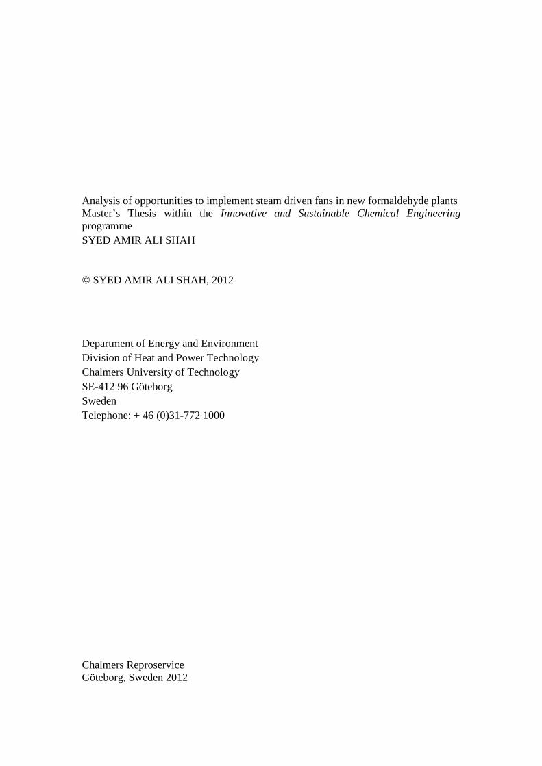
The so-called Balje diagram provides estimates of the total to static efficiencies for compressors and expansion stages. Lower efficiencies (about 3 to 7 %) result for “first built” units. For the convenience of application, a distinction is made between the machines using gases and liquids. Additionally, lines of constant optimum geometry can be plotted for constant values of hub ratio λ (e.g. the lines of constant λ values for axial turbines). Figure 5.2Figure 5.2 shows lines of constant total to static efficiencies for different turbine and expander types as a function of specific speed and specific diameter operating with compressible media at a machine Reynolds number of 2*106.

Higher efficiencies are obtained at specific speeds between 0.5 and 1.0. Single stage axial as well as radial full admission turbines cover this regime equally well. At higher or lower specific speeds the efficiency potential tends to decrease. For specific speeds below 0.1, partial admission turbines offer a higher efficiency potential than full admission turbines. Terry turbines have a lower efficiency potential than the partial admission axial turbines. Rotary displacement type expanders (multilobe) show higher efficiency in the low specific speed regime than dynamic machines. In general, for the dynamic type turbine the specific diameter tends to be higher than displacement type machines. Since the Mach number has a little influence on turbine so the same efficiencies can be obtained with higher or lower Mach number. There is also small increase in efficiency with increasing Reynolds number. The cross flow turbine covers a wide range of specific speeds, thus large specific speeds can be accommodated with small specific diameter. (Turbomachines)

29

Figure 5.2 nsds diagram for single stage turbine and expanders operating with compressible fluids (Turbomachines)

A similar diagram is shown also for compressor stage in Figure 5.3. For dynamic machines highest efficiencies are obtained at specific speeds between 0.5 and 1.0 and the efficiency decreases generally with increasing or decreasing specific speeds. In the high specific speed regime axial compressor have higher efficiencies. Where-as radial compressors give better performance at low specific speeds. Mixed flow type compressors cover the specific speed regime between 1.0 and 2.0 best. For low specific speeds (ns<0.2), partial emission compressors merit consideration, however they only offer a limited efficiency potential. There is definite limit exists for the applicability of single stage dynamic type machines. This limit can be identified by limiting head coefficient. When head coefficient exceeds values of 1.0 then usually extremely low efficiencies are obtained. This limit is identified by a dashed line in Figure 5.3, meaning that in the operating regime to the left of the dashed line, positive displacement machines or hybrid machines (drag pumps) offer a better performance. At very high specific speeds the cross flow blower offers a fair efficiency potential. (Turbomachines)

30

Figure 5.3 nsds diagram for single stage compressor (Turbomachines)

5.2 Estimation of practical potential of electricity generation In the following section practical potential of power generation from the steam turbine and different configurations of steam driven blowers will be discussed.

5.2.1 Super heater The steam for power production application must be superheated before expansion in order to avoid water droplets at the turbine outlet and in order to exploit a larger enthalpy drop for the given pressure ratio.

The following assumptions and data were used to calculate the practical potential of superheated steam according to the new process arrangement as shown in Figure 5.1. The data below is obtained from mass and energy balance,

Mass flow of feed water, m = 631 kg/hr Specific heat of water, Cp= 4,226 kJ/kg.K Feed water inlet temperature, Tin= 105℃ Feed water outlet temperature, Tout= 224℃ Pressure of feed water, P= 26 bara Heat of vaporization, ΔH = 1840 kJ/kg (Wester, Oktober 1996).

𝑄 = 𝑚 ∗ 𝐶𝑝 ∗ 𝛥𝑇 + 𝑚 ∗ 𝛥𝐻 (5.1) Heat load of Super heater is 410 kW.

31

Saturated steam coming from HTF Condenser (from the mass and energy balance); Inlet temperature of Saturated steam, Tin= 224℃ Inlet pressure of Saturated steam, Pin= 25 bara Enthalpy of Saturated steam, hin= 2802 kJ/kg (at Pin and Tin) Mass flow of Saturated steam, m= 3390 kg/hr

𝑄 = 𝑚 ∗ 𝛥𝐻 (5.2) 𝑄 = 𝑚 ∗ (ℎ𝑜𝑢𝑡 − ℎ𝑖𝑛) (5.3)

ℎ𝑜𝑢𝑡 =𝑄𝑚

+ ℎ𝑖𝑛 (5.4)

Outlet enthalpy comes out to be 3237 kJ/kg The outlet temperature of superheated steam from steam library at (Pin, hout) is 399℃.

5.2.2 Concise overview of steam turbines There are some advantages of back-pressure turbine over a condensing turbine, (Steam Turbine and Turboexpanders - chapter-8, 1997).

• Lowest in capital cost • Most suitable for high speeds • Simplest in construction and more reliable

There are also some advantages of condensing steam turbine which are; • Control is easier because it requires less change in live steam for different loads • The enthalpy drop across the turbine is larger so it requires less live steam for a given

power output

The condensing turbine has some disadvantages as compared to back-pressure turbine,

• Longer blades due to high steam volumes • Lower over-all reliability because of the need to provide condenser • High initial cost due mainly to two factors:

a) Large turbine due to high specific volume b) Extra cost of condenser

• Poor operating cost because two third of the steam heat content is used in heating condenser cooling water

• More costly boiler feed water treatment to remove chlorides, salts and silicates which would otherwise produce deposits or corrosion of the blades

• Failure of blades

5.2.3 Preliminary estimates of steam turbine power The superheated steam from the super heater enters into the steam turbine. The estimated power from the steam turbine is 247 kW. The detailed calculation for estimation of steam turbine power is given in Appendix 9.2.

32

Figure 5.4 Estimate of practical potential of power output from the steam turbine against with the blower power consumption profile.

It can be seen from Figure 5.4 that the power requirement is not always higher than the power generated by steam turbine. This means that if electricity storage in the batteries is not considered and if electricity is not sold, the steam power production must balance the power requirement. This means that the steam power available during the first 100 days cannot be fully exploited as the required blower power is less than 247kW

After 100 days, according to our hypothesis on catalyst behavior, the steam power is instead insufficient to fulfill the compression power requirement. From this time until catalyst reloading an extra electrical motor is required.

The maximum power of this motor should compensate the final power requirement of air compression with old catalyst which is around 112 kW.

Under this hypothesis, the mechanical energy produced by the steam turbine during the one catalyst charge cycle (240 days) is equal to the area under the surface ABC (1’400’000 kWh) in Figure 5.4. The electricity provided by the motor during the one catalyst charge cycle (240 days) is equal to the area of BCD (175000 kWh).

The net electricity required by blower system which must be provided with the electrical drivers corresponds to 175000 kWh over a typical load.

33

5.3 Screening of the concepts According to the preliminary calculations shown above, the following turbo-machinery configurations are suggested.

5.3.1 Steam driven blowers 5.3.1.1 Double shaft option In this arrangement one recirculation blower is driven by a turbine and the other recirculation blower is driven by an electrical motor. The possible configuration of this system is shown in Figure 5.5.

Figure 5.5 Sketch of double shaft configuration

5.3.1.2 Single shaft configuration In this arrangement, the steam turbine is connected to one or more blowers in the same shaft (running at the same speed) and a motor is also coupled at the other end of the shaft as shown in Figure 5.6.

34

Fresh air

HCHO process

Recirculationblower

M

M

Steam superheater

Saturated steam

Shaft

Controlled extraction

Steam turbine

Product

Atmosphere

Pressurizationblower

ECS unit

Steam net

Figure 5.6 Sketch of single shaft configuration

5.3.2 Separate steam turbine set A third configuration in which steam a turbine is connected with gear box, generator and transformer, as shown in Figure 5.7, appears also among the possible candidate solutions.

The investment cost for this system was estimated from (Chemical Engineering Revamps Boosting Capacity, April 2012) to be roughly double the investment cost for the other two configurations. At 150 ton/day we have low amount of steam available from the process. The possibility of using this configuration is not beneficial for this system. The power production potential from steam turbine is not good enough when we compare savings in terms of revenues. For the time being this configuration is discarded. In future if there is large amount of steam is available from the process, this configuration could be beneficial in terms of higher revenues.

35

Gear Box

Gen MT Transfor

mer

Turbine

25 bar & 400 C

5 bar

Figure 5.7 Example of Steam turbine drives the gear box

Table 5.2 Summary about all the configurations

Double Shaft Configuration

Single shaft configuration

Separate steam turbine set

Investment cost 200’000 € 334’000 € 650’000 €

Revenues 94’000 €/year 146’000 €/year 182’000 €/year

Pros. Invest cost is less Higher efficiencies of turbo machinery,

Less actual power consumption of electrical motor,

More revenues in terms of electricity savings

Beneficial for large plant capacity (e.g. high amount of steam)

Cons. Less efficiency of turbo machinery,

More power consumption of electrical motor required for the first stage

Investment cost is higher

Investment cost is too high

37

6 SOLUTION FROM VENDORS Purchasing cost of equipment was obtained by direct contact with vendors. The different vendors were provided with full specifications for the two possible steam-driven configurations (double shaft and single shaft).

Initially there were around 8 vendors contacted in which 5 vendors provided the estimated quote. The option suggested by the two vendor A and vendor B, were eventually selected as they appeared more technically reliable in terms of the quoted efficiencies for blowers and turbine compared to other vendors.

To obtain precise quotation by the vendors, three plant characteristic operating points were provided (OP1, OP2, and OP3). In reality the performance of the plant changes around the whole year so we took normal gas flow (OP1) as an operating point. Even though the plant performance varies but this operating point will accommodate all the changes. This is the maximum case (OP1). The other two cases related to electrical guarantee gas flow (OP2) and minimum gas flow (OP3).

Table 6.1 Characteristic operating point

Operating conditions

Mass flow [kg/hr]

OP1 Inlet density

[kg/m3]

OP2 Static pressure

inlet [bara]

OP3 Discharge

[bara]

Normal gas flow (+10%),

max dP

23200 1.43 1.313 2.013

Electrical guarantee gas

flow

21000 1.27 1.313 1.763

Min gas flow 12100 1.27 1.163 1.463

While enough indications about performances of the blower stages were attached to such quotations, only few non-relevant indications were provided for the turbine stages. So for the turbines we had to estimate the performances through preliminary considerations. Basically we took mass flow rate of steam and speed of compressor and from the Balje diagrams we estimate specific speed and efficiency of steam turbine.

For this reason, the expected turbine efficiency from the vendor’s quote was verified with Balje diagrams, and accordingly the power requirement profiles for blowers and power production profile from the steam turbine estimated for a typical load.

38

6.1 Vendor A (Double Shaft Configuration) The possible configuration of this system is shown in Figure 5.5. Table 6.2 Data for Centrifugal compressor and turbine from vendor A

Compressor Turbine

Efficiency 75% 40%

Speed 3500 rpm 3500 rpm

6.1.1 Estimation of the blower nominal performances based on the quoted turbo-machinery speed

First we consider single stage compressor The design conditions for Compressors are Pout= 1.313+0.7=2.013 bar Pin= 1.313 bar ρ = 1.43 kg/ m3 m= 21000 kg/hr, V1= 4.08 m3/sec T1= 323K For air, k= 1.4 & Cp = 1.04kJ/kg.k

∆𝐻𝑖𝑠 = 𝐶𝑝.𝑇1. [�𝑝𝑜𝑢𝑡𝑝𝑖𝑛

�𝑘−1/𝑘

– 1] (6.1)

ΔHis= 43.4 kJ/kg For chosen (from the vendor A quoted speed), n= 3500 rpm

𝜔 =2𝜋𝑛60

(6.2)

ω= 366.34 rad/sec

𝑛𝑠 =𝜔.√𝑉1

(∆𝐻𝑖𝑠)0.75 (6.3)

ns = 0.25→ Efficiency of Compressor is 50% (It is too low when we compare efficiency with the vendor’s quote).

Accordingly, two stages must be chosen in order to distribute the desired pressure increase to achieve better performances at the same speed. This confirms the choice of two stages and is at the base of the two shaft configuration. Now if for 2 stage compressor,

ΔHis= 43.4/2 = 21.7 kJ/kg


(∆𝐻𝑖𝑠)0.75 (6.4)

ns = 0.41→ Efficiency of Compressor is 75%. Such value confirms the blower performances quoted by vendor A from Table 6.2.

39

6.1.2 Estimation of the blower power requirement profile based on the quoted characteristic curves

In order to estimate the actual power profile of the two blower stages along the one catalyst charge cycle (240 days), the performance characteristics provided by the vendor for the three typical plant operating point were “collapsed” into single performance curve according to the similarity theory.

This corresponds to plot the non-dimensional head coefficient ψ against the non-dimensional flow coefficient φ where

ψ =𝐷𝐻𝑖𝑠n2D2 (6.5)

φ =𝑉

nD3 (6.6)

According to similarity concepts the non-dimensional head coefficient and the machine efficiency assume equal numerical values in dynamically similar operating point (that is when all fluid velocities at corresponding points within the machine are in the same direction and proportional to the blade speed), resulting in the following type of diagram:

φ

Ψ

η

η

Ψ

Figure 6.1 Non-dimensional flow coefficient φ against non-dimensional head coefficient ψ and efficiency η In quotation from vendor A, the two stages are different so two different non-dimensional curves were built.

In addition, they suggest operating the two stages in such a way that the first stage follows the major part of the increasing total head while the second stage operates almost at constant pressure ratio.

By following such indications, the operating points of the two blowers were estimated. In particular as the required head changes over the time, the speed of the blower’s increases and therefore the non-dimensional flow coefficient diminish as the

40

volumetric flow rate is constant (constant gas flow for nominal plant operation) but the turbo machinery speed increases. Accordingly the efficiency of the machines also changes during the typical year.

It can be seen in the Table 6.3 that the design of double shaft configuration is particularly inefficient when the catalyst is fresh but the performances increases at higher speeds when the catalyst gets older.

Due to increased head of the first stage, the gas density at the second stage inlet progressively increases thus reducing the volumetric flow rate. This causes the second stage performance to be influenced by the first stage.

The speed of revolution of the blower also increases due to higher power requirement, and it is calculated as shown in Table 6.3.

Table 6.3 Calculated blower power requirements for 1st and 2nd stage

1st stage 2nd stage Total blower power

days Δp [bar] n [1/min] power [kW] Eff. n η power [kW] [kW] 0 0,47 3184 154 0,69 3168 0,71 106 261

10 0,471 3186 155 0,69 3168 0,71 106 261 20 0,472 3192 155 0,69 3169 0,71 106 262 30 0,475 3201 157 0,69 3170 0,71 107 263 40 0,479 3214 158 0,69 3172 0,71 107 265 50 0,485 3231 160 0,69 3174 0,71 107 267 60 0,491 3252 163 0,69 3176 0,71 108 270 70 0,499 3276 166 0,69 3179 0,71 108 274 80 0,508 3303 169 0,69 3182 0,71 108 278 90 0,519 3334 173 0,69 3185 0,72 109 282

100 0,530 3369 178 0,70 3188 0,72 110 287 110 0,543 3406 182 0,70 3191 0,72 110 293 120 0,557 3447 187 0,70 3195 0,72 111 298 130 0,572 3491 193 0,70 3199 0,72 112 305 140 0,589 3538 199 0,70 3206 0,73 113 311 150 0,606 3587 205 0,71 3214 0,73 114 319 160 0,625 3639 211 0,71 3222 0,73 115 326 170 0,645 3694 218 0,71 3230 0,74 116 334 180 0,666 3751 225 0,72 3238 0,74 117 342 190 0,689 3810 233 0,72 3245 0,74 118 351 200 0,713 3871 241 0,72 3251 0,74 119 359 210 0,738 3934 248 0,73 3260 0,75 120 368 220 0,764 3998 257 0,73 3270 0,75 121 378 230 0,791 4064 265 0,73 3281 0,75 122 387 240 0,820 4131 273 0,74 3290 0,76 124 397

41

Figure 6.2 Blower power profile for a typical load

6.1.3 Preliminary estimation of the turbine performance based on the quoted nominal speed

The type of steam turbine used by vendor A is partial admission axial type and this is confirmed by looking at the Balje diagrams for the corresponding specific speed and specific diameters.

Design conditions for Turbine Pout= 5 bar Pin= 25 bar T1= 400°C ρ at (5bar & 270°C) = 2.03 kg/ m3 m= 3390 kg/hr, V1= 0.464 m3/sec From the Mollier Diagram ΔHis= 405 kJ/kg For a preliminary value of the nominal speed of 3500 rpm

𝜔 =2𝜋𝑛60

(6.7)

ω= 366.34 rad/sec


(∆𝐻𝑖𝑠)0.75 (6.8) ns = 0.015→ Efficiency of Steam Turbine is 40%.

42

This very low turbine efficiency value is confirmed from the Balje diagrams for vendor A as shown in Table 6.2.

The procedure for the preliminary design of turbine is summarized in the table below. In particular it was assumed that the nominal rotational speed is the maximum rotational speed for the blower stage coupled with the turbine (3290 rpm).

Under this assumption, the isentropic spouting velocity c0 is calculated and the ratio between the tangential velocity u (calculated by selecting the appropriate machine diameter from Balje diagrams) and c0 estimated.

Table 6.4 Preliminary turbine design

average n blowers 3208 max n blower 3289

n_design 3290

ω [rad/s] 344,5

p0 [bar] 25

h0 [kJ/kg] 3239 p2 [bar] 5

s0[kJ/kgK] 7,0

T0 [degC] 400

h2is[kJ/kg] 2835

Δhis[kJ/kg] 404

m [kg/s] 0,94

c0 [m/s] 899

1 stage

guess values check the calculations with results from Balje ηis 0,4

Δh [kJ/kg] 161

h2 [kJ/kg] 3078

s2 [kJ/kg] 7,4

T2 [degC] 306,5

ρ [m3/kg] 1,89

V2 [m3/s] 0,49

ns 0,01

0,015149 1

0,015149 100

from Balje

ds 35

ηis 0,4

D [m] 0,97

for values higher than 300 check stress ! u [m/s] 168

43

u/c0 0,18

c* [m/s] 585 check flow is choked

Mach guess 1,53

objective: keep the same u/c0 to keep high the turbine efficiency

6.1.4 Estimation of the turbine power based on the obtained blower shaft speed

The ratio (u/c0) defines the operating point of maximum turbine performance and should be therefore kept constant during turbine operation.

As the shaft speed changes according to the increasing head that the blower has to provide, the isentropic spouting velocity c0 must therefore be adjusted to keep the turbine in high performance regimes.

This must be done by adjusting the inlet pressure p0 available at the turbine inlet. In particular, if this is equal to 25 bar when the turbine is operating at maximum power (old catalyst), the pressure at the turbine inlet is much lower at lower powers (new catalyst).

This also causes the specific work of the turbine stage to change as a consequence of the changing available theoretical head, so the required power can be provided by admitting more or less steam.

In fact, at the turbine inlet the flow is chocked (M=1), which means that for each inlet nozzle a given constant steam flow rate is admitted. Accordingly, the mass flow rate can be changed only by adjusting the partial admission that is by opening or closing some inlet nozzles.

The remaining mass flow rate that is not required for power generation is throttled directly to the low pressure and used for heating purposes.

In Table 6.5 the turbine operation during the typical load is described.

44

Table 6.5 Turbine power for 2nd stage

turbine

from blower turbine throttle to heating

days

n [rev/min]

p0 [bar]

power req [kW]

m [kg/s] m [kg/s] Q [kW]

Heating [kWh]

0 3168 22 106 0,71 0,23 2487 0 10 3168 22 106 0,71 0,23 2487 596880 20 3169 22 106 0,71 0,23 2487 596880 30 3170 22 107 0,71 0,23 2487 596880 40 3172 22 107 0,71 0,23 2486 596640 50 3174 22 107 0,71 0,23 2486 596640 60 3176 22 108 0,71 0,23 2486 596640 70 3179 22 108 0,71 0,23 2485 596400 80 3182 22 108 0,72 0,23 2485 596400 90 3185 22 109 0,72 0,22 2484 596160

100 3188 22 110 0,72 0,22 2484 596160 110 3191 22 110 0,72 0,22 2483 595920 120 3195 22 111 0,73 0,21 2482 595680 130 3199 23 112 0,73 0,21 2482 595680 140 3206 23 113 0,73 0,21 2481 595440 150 3214 23 114 0,74 0,21 2480 595200 160 3222 23 115 0,74 0,20 2479 594960 170 3230 23 116 0,74 0,20 2478 594720 180 3238 24 117 0,74 0,20 2477 594480 190 3245 24 118 0,75 0,19 2476 594240 200 3251 24 119 0,75 0,19 2475 594000 210 3260 24 120 0,76 0,19 2474 593760 220 3270 24 121 0,76 0,18 2472 593280 230 3281 25 122 0,76 0,18 2471 593040 240 3290 25 124 0,76 0,18 2470 592800

total 14288880

45

Figure 6.3 Steam turbine power profile (Blower 2nd stage is connected with the steam turbine)

6.1.5 Electricity savings The theoretical electricity savings and the required power of the electrical motor for the first stage are given in Table 6.6. Initially we did all the calculations for one catalyst cycle (240 days). In order to calculate annual electricity savings for 350 days we multiply the theoretical electricity savings by a factor of (350 days/240 days) 1.46. The total theoretical electricity savings is then 940’000 kWh/year. The total electricity consumption is 2’600’000 kWh/year.

46

Table 6.6 Electricity savings for the double shaft case over a typical load

Days Total Shaft Power (kW)

Steam Power for 2nd stage

(kW)

Theoritical Electrical Saving (kWh)

Electricity Consumption (kWh)

Actual power consumption of Electrical Motor for 1st stage (kW)

0 260 106 0 0 154 10 261 106 25440 62640 155 20 261 106 25440 62640 155 30 263 106 25440 63120 157 40 265 107 25680 63600 158 50 267 107 25680 64080 160 60 270 107 25680 64800 163 70 273 108 25920 65520 165 80 277 108 25920 66480 169 90 282 109 26160 67680 173

100 287 109 26160 68880 178 110 292 110 26400 70080 182 120 298 111 26640 71520 187 130 304 112 26880 72960 192 140 311 113 27120 74640 198 150 318 113 27120 76320 205 160 326 114 27360 78240 212 170 333 115 27600 79920 218 180 342 116 27840 82080 226 190 350 118 28320 84000 232 200 359 119 28560 86160 240 210 368 120 28800 88320 248 220 378 121 29040 90720 257 230 387 122 29280 92880 265 240 397 124 29760 95280 273

648240 1792560

47

Figure 6.4 Turbo machinery power profile over a typical load

Table 6.7 Summary about double shaft configuration

Double shaft configuration

Steam available for sale in the reference plant (For a steam price of 20€/ton of steam) Appendix 9.4

675’000 €/year

Steam available for sale in the double shaft configuration (For a steam price of 20€/ton of steam) Appendix 9.4

645’000 €/year

Electricity generation 940’000 kWh/year

Cash flows 94’000 €/year

6.1.6 Profitability analysis 6.1.6.1 Investment cost The investment cost was obtained from the direct contact with vendors. The investment cost for the double shaft configuration was estimated to be 200’000 €/unit. This investment cost includes the super heater, piping, valves, engineering cost, controls, and contingency.

48

6.1.6.2 Annual savings The annual savings is calculated from the available steam turbine power. The price of electricity is assumed to be 0.1 €/kWh. The savings for the double shaft case is 94’000 €.

6.1.6.3 Payback time The time elapses from the start of the project to the breakeven point. The shorter is the payback time the more attractive is the project.

𝑃𝐵𝑇

=𝐼𝑛𝑣𝑒𝑠𝑡𝑚𝑒𝑛𝑡

𝐴𝐶𝐹 (𝐴𝑛𝑛𝑢𝑎𝑙 𝐶𝑎𝑠ℎ 𝐹𝑙𝑜𝑤) (6.9)

6.1.6.4 Net present value The effect of time on the value of money is taken into account by discounting the annual cash flow ACF with the rate of interest to obtain annual discounted cash flow ADCF. The sum of ΣADCF over 10 years is known as NPV.

𝑁𝑃𝑉 = � 𝐷𝑖𝑠𝑐𝑜𝑢𝑛𝑡𝑒𝑑 𝑐𝑎𝑠ℎ 𝑓𝑙𝑜𝑤𝑦𝑒𝑎𝑟 – 𝐼𝑛𝑖𝑡𝑖𝑎𝑙 𝐼𝑛𝑣𝑒𝑠𝑡𝑚𝑒𝑛𝑡 𝑐𝑜𝑠𝑡 (6.10)10

𝑦𝑒𝑟𝑎=0

The greater the positive NPV for a project, the more attractive is the investment.

6.1.6.5 Electricity prices Different prices of electricity were taken into account in order to estimate the profitability of the different configurations if they were to be implemented in different countries.

Figure 6.5 Electricity prices in different countries (Portel, 2011) Without considering the economic value of heat sales from the double shaft case, the profitability analysis is given in Figure 6.6. The revenues in the table below came from the electricity savings.

49

Table 6.8 Investment and Revenues for double shaft configuration

Price of electricity 0.1 €/kWh

Electricity savings 940’000 kWh/year

Investment 200’000 €

Revenues 94’000 €/year

Figure 6.6 Profitability analysis without heat sales

If we consider economic value of heat sales, as a comparison of the double shaft case with the standard case the difference will be the loss of money that is 30000 €/year. Appendix 9.4

So the revenues from the double shaft configuration is 64000 €/year, shown in Figure 6.7.

50

Figure 6.7 Profitability analysis with considering heat sales

6.2 Vendor B (Single Shaft Configuration) The method from (Turbomachines) used to verify the performances of compressors and turbine for double shaft is also used to verify the performances for single shaft configuration and to estimate the actual system operation during the one catalyst charge cycle (240 days). The possible configuration of this system is shown in Figure 5.6. The turbo machinery speed in the single shaft case is much higher than in the double shaft case, so higher efficiencies are expected from the Balje diagrams. Table 6.9 Data for Centrifugal compressor and turbine from vendor B

Compressor Turbine

Efficiency 85% 60%

Speed 12000 rpm 12000 rpm

51

6.2.1 Estimation of the blower nominal performances based on the quoted turbo-machinery speed

First we consider single stage compressor

Design conditions for Compressors

Pout= 1.313+0.7=2.013 bar

Pin= 1.313 bar

ρ = 1.43 kg/ m3

m= 21000 kg/hr, V1= 4.08 m3/sec

T1= 323K

For air, k= 1.4 & Cp = 1.04kJ/kg.k

∆𝐻𝑖𝑠 = 𝐶𝑝.𝑇1. [�𝑝𝑜𝑢𝑡𝑝𝑖𝑛

�𝑘−1/𝑘

– 1] (6.11)

ΔHis= 43.4 kJ/kg

For chosen (from the vendor B quoted speed), n= 12000 rpm

𝜔 =2𝜋𝑛60

(6.12)

ω= 1256 rad/sec


(∆𝐻𝑖𝑠)0.75 (6.13)

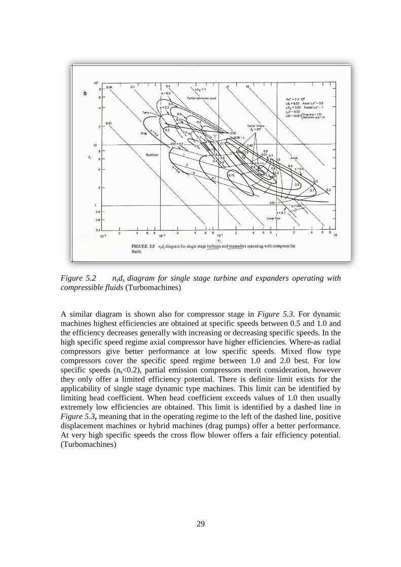
ns = 0.84→ Efficiency of Compressor is 85%. Such value is confirmed by vendor B as shown in Table 6.9.

6.2.2 Estimation of the blower power requirement profile based on the quoted characteristic curves.

In quotation from vendor B, they have only one stage so only one dimensional curve was built. The speed of revolution of the blower is also quite high, so they can handle all the head requirements in a single stage.

In addition, they suggest operating the single stage in such a way that blower, turbine and motor are connected on a single shaft. In particular as the required head changes over the time, the speed of the blower increases and therefore the non-dimensional flow coefficient diminish as the volumetric flow rate is constant (constant gas flow for nominal plant operation) but the turbo machinery speed increase. Accordingly the efficiency of the machines also changes during the typical year.

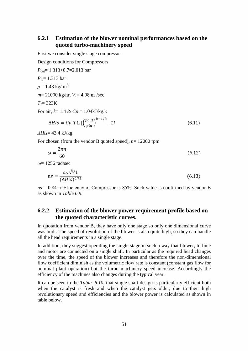
It can be seen in the Table 6.10, that single shaft design is particularly efficient both when the catalyst is fresh and when the catalyst gets older, due to their high revolutionary speed and efficiencies and the blower power is calculated as shown in table below.

52

Table 6.10 Calculated blower power requirements

days Δp [bar] n [rev/min] η Total blower power [kW]

0 0,470 10212 0,789 227 10 0,470 10215 0,790 228 20 0,472 10230 0,790 228 30 0,475 10256 0,790 230 40 0,479 10295 0,791 231 50 0,485 10330 0,791 233 60 0,491 10385 0,792 236 70 0,499 10445 0,793 239 80 0,508 10520 0,794 243 90 0,519 10595 0,794 247

100 0,538 10680 0,795 252 110 0,543 10780 0,796 257 120 0,557 10880 0,796 263 130 0,572 11000 0,796 269 140 0,589 11110 0,796 276 150 0,606 11240 0,796 283 160 0,625 11370 0,796 291 170 0,645 11510 0,795 299 180 0,666 11660 0,795 308 190 0,689 11800 0,793 317 200 0,713 11970 0,792 327 210 0,738 12120 0,790 338 220 0,764 12290 0,788 349 230 0,791 12460 0,786 361 240 0,820 12635 0,784 373

53

Figure 6.8 Blower power profile

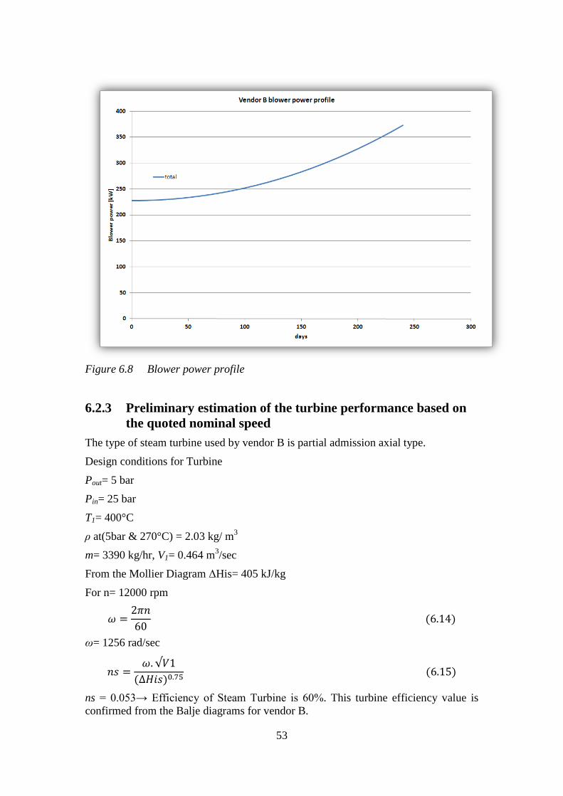
6.2.3 Preliminary estimation of the turbine performance based on the quoted nominal speed

The type of steam turbine used by vendor B is partial admission axial type.

Design conditions for Turbine

Pout= 5 bar

Pin= 25 bar

T1= 400°C

ρ at(5bar & 270°C) = 2.03 kg/ m3

m= 3390 kg/hr, V1= 0.464 m3/sec

From the Mollier Diagram ΔHis= 405 kJ/kg

For n= 12000 rpm

𝜔 =2𝜋𝑛60

(6.14)

ω= 1256 rad/sec


(∆𝐻𝑖𝑠)0.75 (6.15)

ns = 0.053→ Efficiency of Steam Turbine is 60%. This turbine efficiency value is confirmed from the Balje diagrams for vendor B.

54

Table 6.11 Preliminary turbine design

average n blowers 11079 ω [rad/s] 1323 max n blower 12635

n_design 12635 h0 [kJ/kg] 3239

s0 [kJ/kg-K] 7,0

p0 [bar] 25 h2is [kJ/kg] 2835 p2 [bar] 5 Δhis [kJ/kg] 404 T0 [degC] 400

c0 [m/s] 899 m [kg/s] 0,94

guess values

ηis 0,61

Δh [kJ/kg] 246

h2 [kJ/kg] 2993

s2 [kJ/kg] 7,3

T2 [degC] 265

ρ [m3/kg] 2,0

V2 [m3/s] 0,46

ns 0,05

from Balje

ds 17

ηis 0,61

D [m] 0,45

u [m/s] 302,6

u/c0 0,33

c* [m/s] 564,4

Mach guess 1,59

55

6.2.4 Estimation of the turbine power based on the obtained blower shaft speed

As the shaft speed changes according to the increasing head that the blower has to provide, the isentropic spouting velocity c0 must therefore be adjusted to keep the turbine in high performance regimes.

This must be done by adjusting the mass flow rate that gives inlet pressure p0 available at the turbine inlet. In particular, if this is equal to 25 bar when the turbine is operating at maximum power (old catalyst), the pressure at the turbine inlet is much lower at lower powers (new catalyst).

In fact, at the turbine inlet the flow is choked (M=1), which means that for each inlet nozzle a given constant steam flow rate is admitted. Accordingly, the mass flow rate can be changed only by adjusting the partial admission that is by opening or closing some inlet nozzles.

The remaining mass flow rate that is not required for power generation is throttled directly to the low pressure and used for heating purposes.

As the speed of revolution in case of single shaft is higher than double shaft, so steam turbine is generating more power. Due to their high revolutionary speed, their efficiencies are also higher than double shaft.

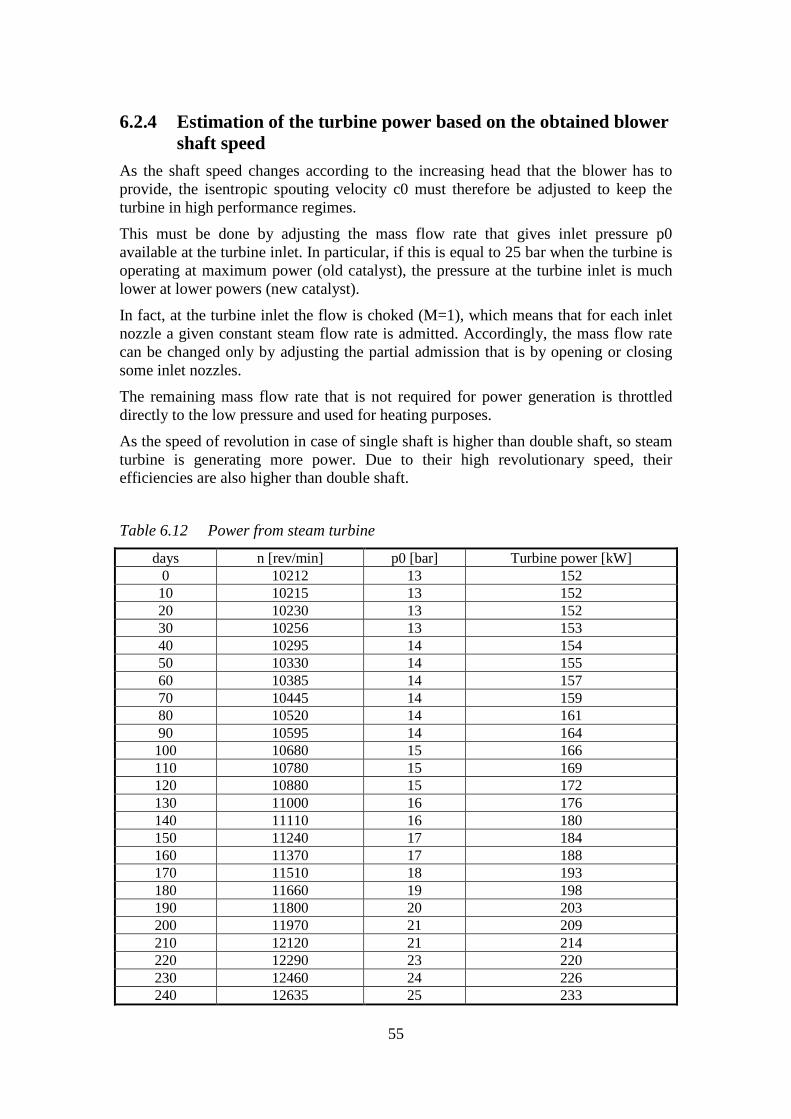
Table 6.12 Power from steam turbine

days n [rev/min] p0 [bar] Turbine power [kW] 0 10212 13 152

10 10215 13 152 20 10230 13 152 30 10256 13 153 40 10295 14 154 50 10330 14 155 60 10385 14 157 70 10445 14 159 80 10520 14 161 90 10595 14 164

100 10680 15 166 110 10780 15 169 120 10880 15 172 130 11000 16 176 140 11110 16 180 150 11240 17 184 160 11370 17 188 170 11510 18 193 180 11660 19 198 190 11800 20 203 200 11970 21 209 210 12120 21 214 220 12290 23 220 230 12460 24 226 240 12635 25 233

56

How the turbine power profile varies with time is shown in Figure 6.9.

Figure 6.9 Turbine power profile

6.2.5 Electricity savings The electricity savings and the power required by the electrical motor are given in Table 6.6 and Table 6.13. Initially we did all the calculations for one catalyst cycle (240 days). In order to calculate annual electricity savings for 350 days we multiply the theoretical electricity savings by a factor of (350 days/240 days) 1.46. The total theoretical electricity savings from single shaft configuration is 1’460’000 kWh/year. The total electricity consumption for single shaft configuration is 2’240’000 kWh/year. The theoretical electrical savings are more in single shaft configuration than in the double shaft configuration; also with single shaft system actual power consumption of electrical motor is less than the double shaft system.

57

Table 6.13 Electricity savings for single shaft case over a typical load

days Total shaft power (kW)

Turbine power for

blower (kW)

Theoritical Electrical Saving

(kWh)

Electricity Consumption

(kWh)

Actual power

consumption of electrical motor (kW)

0 227 152 0 0 75 10 228 152 36480 54720 76 20 228 152 36480 54720 76 30 230 153 36720 55200 76 40 231 154 36960 55440 77 50 233 155 37200 55920 78 60 236 157 37680 56640 79 70 239 159 37920 57360 80 80 243 161 38640 58320 82 90 247 164 39120 59280 84 100 252 166 39840 60480 86 110 257 169 40560 61680 88 120 263 172 41280 63120 90 130 269 176 42240 64560 93 140 276 180 42960 66240 96 150 283 184 44160 67920 99 160 291 188 45120 69840 102 170 299 193 46080 71760 106 180 308 198 47520 73920 110 190 317 203 48480 76080 115 200 327 209 49920 78480 119 210 338 214 51120 81120 124 220 349 220 52800 83760 129 230 361 226 54240 86640 135 240 373 233 55680 89520 140

1039200 1602720

58

Figure 6.10 Turbo machinery power profile over a typical load

Table 6.14 Summary about Single shaft configuration


Steam available for sale in the reference plant (For a steam price of 20€/ton of steam) Appendix 9.4

675’000 €/year

Steam available for sale in the Single shaft configuration (For a steam price of 20€/ton of steam) Appendix 9.4

630’000 €/year

Electricity generation 1’460’000 kWh/year

Cash flows 146’000 €/year

6.2.6 Profitability analysis Investment cost is obtained by the direct contact with vendors. The investment cost from the vendor is 334’000 €/unit. This investment cost includes the super heater, piping, valves, engineering cost, controls, and contingency. The annual savings is calculated from the available steam turbine power. The price of electricity is assumed to be 0.1 €/kWh. The annual savings in case of single shaft case is 146’000 €.

If we do not consider the economic value of heat sales from the single shaft case than profitability analysis is shown in Figure 6.11.

59

Table 6.15 Investment and Revenues for single shaft configuration

Price of electricity 0.1 €/kWh

Electricity savings 1’460’000 kWh/year

Investment 334’000 €

Revenues 146’000 €/year

Figure 6.11 Profitability analysis without heat sales If we consider the economic value of heat sales than 45700 € money is lost every year. So the revenues from the single shaft configuration is 100’000 €/year, which is given in Figure 6.12.

60

Figure 6.12 Profitability analysis with considering heat sales

61

7 SUMMARY OF RESULTS AND CONCLUSION

7.1 Electricity savings and profitability Table 7.1 Yearly shaft work available from the turbine

Double shaft configuration

(kWh)


(kWh)

Pinch analysis methodology

(kWh)

940’000 1’460’000 2’620’000

Table 7.2 Profitability analysis without heat sales

Double shaft configuration Single shaft configuration

NPV (i=5%) 420’000 € 640’000 €

PBT (i=5%) 3.0 year 3.4 year

NPV (i=10%) 300’000 € 420’000 €


Table 7.3 Profitability analysis with heat sales

Double shaft configuration Single shaft configuration

NPV (i=5%) 240’000 € 350’000 €


NPV (i=10%) 160’000 € 220’000 €


Table 7.4 Summary about all configurations

Double Shaft Configuration Single shaft configuration

Lifetime of plant 10 years 10 years

Investment cost 200’000 € 334’000 €

Revenues 94’000 €/year 146’000 €/year

Steam available for sale 645’000 €/year 630’000 €/year

62

7.2 Conclusion In this thesis different configurations of turbo machinery have been investigated for power generation from the process excess heat. The energy analysis for this thesis was carried out using Pinch Technology in order to gather all the necessary stream data and investigate the potential for energy recovery.

The practical aspect of energy recovery through steam-driven recirculation blowers were discussed in detail.

Turbo machinery similarity theory and, in particular, Balje diagrams were used to performed preliminary selection of the required machines and the quotation from vendors were used to make estimation of the steam-driven system over a typical year of plant operation.

An economic analysis for the different configurations was carried out.

In the current plant with a nominal capacity of 150 ton/day, the plant produces 3390 kg/hr saturated steam at 25 bar from the excess process heat. This steam, in the current standard design, is sold to nearby industrial process.

It is in the interest of the company to propose a design in which this steam is internally used. A preliminary calculation shows that 247 kW power output from a steam turbine is possible in nominal plant condition.

From the Pinch Analysis consideration, a higher amount of steam appears potentially available (4300 kg/hr) including super heater which can possibly correspond to the 312 kW of power if the same steam pressure is used as in the standard plant, which is around 70 kW more than what is practically achievable if no major plant re-design is carried out.

The total blower power requirement in the case of single shaft is lower than double shaft. We need to have an electrical motor in order to meet the blower power requirement when the catalyst is getting old. Thus the size of an electrical motor is also smaller and the available power from the steam turbine is also higher in single shaft configuration than double shaft. This is due to the fact that turbo machinery in single shaft configuration operates at a higher speed thus allowing much higher efficiencies of their machines.

The economic evaluations of the thesis were carried out with different interest rates and an economic lifetime of 10 years. The investment cost for the different configuration of turbo machinery was taken from the vendors.

The pay-back period investigations indicate a minimum payback period of around 3 years (for single and double shaft configuration) for a electricity price of 0.1 €/kWh, but the net present value is higher in single shaft configuration than double shaft at the end of 10 year. Even though the investment cost is higher in single shaft configuration than double shaft configuration. The revenues in terms of electricity savings is also more in single shaft configuration therefore single shaft solution is preferred.

63

8 REFERENCES Cardu, M. (1993). Thermal Power Rational Management Using Backpressure Steam Turbine. Romania: Institute of Scientific Research and Technological Engineering for Power Equipment (ICSITEE).

Chemical Engineering Revamps Boosting Capacity. (April 2012).

Cheng - Liang Chen, C. -Y. (2011). A flexible structural and operational design of steam systems. Taiwan: Department of Chemical Engineering, National Taiwan University.

Cotton, K. (1993). Evaluating and Improvement Steam Turbine Performance. Gilson Work.

Fans, A. F. (1997). Handbook of Modern Fan Technology. Fans, ABB Fläkt Oy Industrial.

Formox, P. (2006). Operating Manual. Perstorp: Perstorp.

Hagman, H., & Walhelm, M. (2005). Implementation of a turboexpander in Perstorp Formox's Formalin Process. Lund, Sweden: Lund Institute of Technology.

Harvey, S. (2009). Industrial Energy System - course compendium. Göteborg, Sweden: Chalmers University Of Technology (Department of Energy and Environment. Division of Heat and power Technology).

Inc., B. N. (2012). Retrieved from http://www.barber-nichols.com

Kemp, I. C. (2007). Pinch Analysis and Process Integration. Elsevier Ltd.

Piller. (2012). Retrieved from www.piller.com

Portel, E. E. (November 2011). Hämtat från Fuel Prices: http://www.energy.eu/

Sons, J. W. Energy Management. Krik - Othmer Encyclopedia of Chemical Technology. Vol. 10.

Steam Turbine and Turboexpanders - chapter-8. (1997).

Svensson, E. (2008). Optimization of Process Integration Investments under Energy Market Uncertainties. Göteborg, Sweden: Chalmers University of Technology: Department of Energy and Environment (Division of Heat and Power Technology).

Turbomachines, O. B. " A guide to design, selection, and theory.

Wester, L. (Oktober 1996). Tabeller och Diagram for energitekniska beräkningar.

65

9 APPENDIX

9.1 Estimation of Blower Power 1st stage calculations Density of gas before recirculation blowers, ρo =kg/m3

Inlet volumetric flow rate to the recirculation blowers, Vo = 4,08 m3/sec

Inlet mass flow rate to the recirculation blowers, m = 5,8 kg/sec

Inlet pressure of gas before recirculation blowers, P0 = 1,3 bara

Inlet temperature of gas before recirculation blowers, T0 = 38℃ Heat capacity ratio for air, κ = 1,4

Specific heat of air, Cp = 1,009 kJ/kg

For fresh catalyst the outlet pressure from the 2nd stage, P2 (set) = 1,78 bara

Pressure increases across 2nd stage is

𝛥𝑃2 =𝑃2 − 𝑃𝑜

1,8+ 0,005 (9.1)

ΔP2= 0,272 bara

Pressure increases across 1st stage

𝛥𝑃1 = (𝑃2 − 𝑃𝑜) − 𝛥𝑃2 + 0,005 (9.2) ΔP1= 0,213 bara

Outlet pressure from the 1st stage, P1

𝑃1 = 𝑃𝑜 + 𝛥𝑃1 (9.3) P1 = 1,513 bara

For the adiabatic process, see Figure 3.2

S (kJ/kg/K)

H (kJ/kg)

h1

h2is

h2

p2

p1

T1

T2S

T2

Figure 9.1 Adiabatic process

𝑇1𝑠𝑇𝑜

= �𝑃1𝑃𝑜�𝜅−1/𝜅

(9.4)

66

𝑇1𝑠 = 𝑇𝑜 �𝑃1𝑃𝑜�𝜅−1/𝜅

(9.5)

T1s = 51,8 ℃

ℎ1𝑠 = 𝐶𝑝 ∗ 𝑇1𝑠 (9.6) h1s = 327,7 kJ/kg

ℎ𝑜 = 𝐶𝑝 ∗ 𝑇𝑜 (9.7) h0 = 313,8 kJ/kg

𝛥𝐻 = ℎ1𝑠 − ℎ𝑜 (9.8) ΔH = 13,92 kJ/kg

The efficiency of the fan is assumed to be constant 79 % (including all bearings and couplings losses) and the shaft power of fan from the first stage comes out to be (Fans, 1997).

𝑃 =𝑉𝑜 ∗ 𝛥𝐻 ∗ 𝜌𝑜

𝜂 (9.9)

P = 103 kW

2nd stage calculations For the 2nd stage, the Inlet pressure, = Outlet pressure from 1st stage, P1 = 1,51 bara

𝜂 =𝐶𝑝 ∗ (𝑇1𝑠 − 𝑇𝑜)𝐶𝑝 ∗ (𝑇1 − 𝑇𝑜)

(9.10)

The outlet temperature from the 1st stage will be

𝑇1 =(𝑇1𝑠 − 𝑇𝑜)

𝜂+ 𝑇𝑜 (9.11)

T1 = 55,5 ℃ after the 1st stage The inlet density to the 2nd stage,

𝜌1 =𝑃1 ∗ 𝑇𝑜 ∗ 𝜌𝑜𝑇1 ∗ 𝑃𝑜

(9.12)

ρ1 = 1,576 kg/m3

Volumetric flow rate to 2nd stage, V1 = m/ρ1

V1 = 3,70 m3/sec

The outlet pressure from the 2nd stage is

𝑃2 = 𝑃1 + 𝛥𝑃2 − 0,005 (9.13) P2 = 1,78 bara

𝑇2𝑠 = 𝑇1 �𝑃2𝑃1�𝜅−1/𝜅

(9.14)

T2s = 71,1 ℃

ℎ2𝑠 = 𝐶𝑝 ∗ 𝑇2𝑠 (9.15)

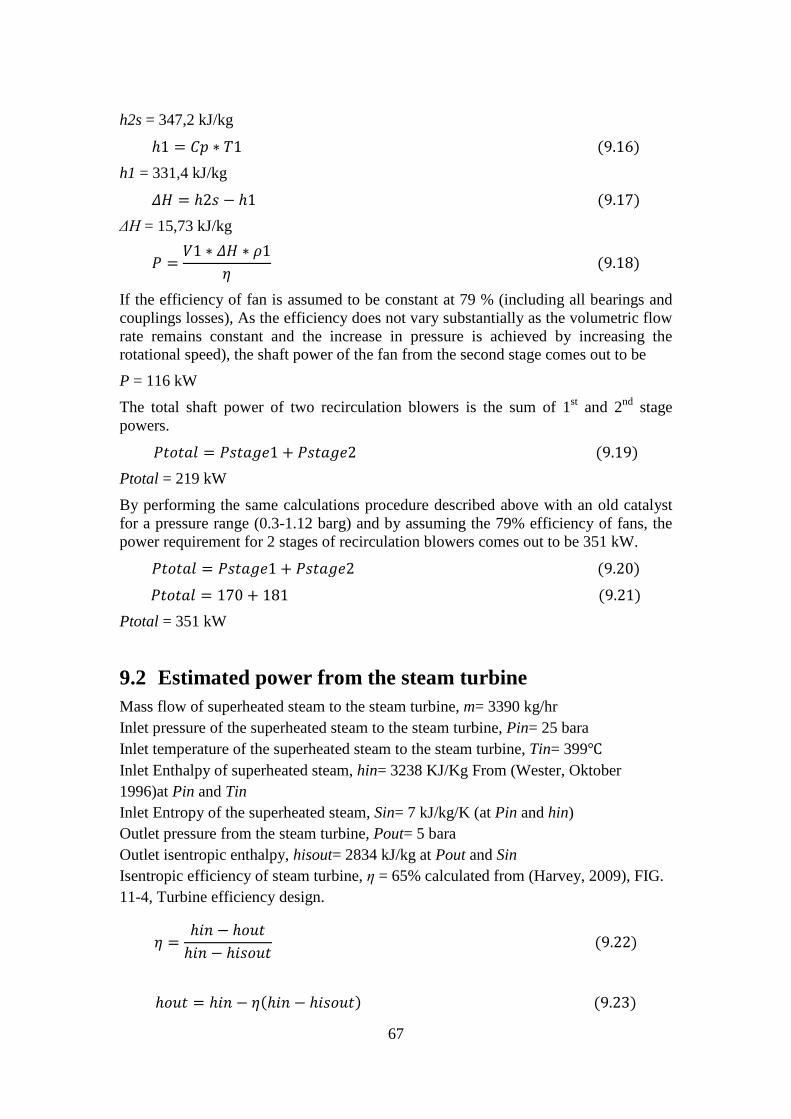
67

h2s = 347,2 kJ/kg

ℎ1 = 𝐶𝑝 ∗ 𝑇1 (9.16) h1 = 331,4 kJ/kg

𝛥𝐻 = ℎ2𝑠 − ℎ1 (9.17) ΔH = 15,73 kJ/kg

𝑃 =𝑉1 ∗ 𝛥𝐻 ∗ 𝜌1

𝜂 (9.18)

If the efficiency of fan is assumed to be constant at 79 % (including all bearings and couplings losses), As the efficiency does not vary substantially as the volumetric flow rate remains constant and the increase in pressure is achieved by increasing the rotational speed), the shaft power of the fan from the second stage comes out to be

P = 116 kW

The total shaft power of two recirculation blowers is the sum of 1st and 2nd stage powers.

𝑃𝑡𝑜𝑡𝑎𝑙 = 𝑃𝑠𝑡𝑎𝑔𝑒1 + 𝑃𝑠𝑡𝑎𝑔𝑒2 (9.19) Ptotal = 219 kW

By performing the same calculations procedure described above with an old catalyst for a pressure range (0.3-1.12 barg) and by assuming the 79% efficiency of fans, the power requirement for 2 stages of recirculation blowers comes out to be 351 kW.

𝑃𝑡𝑜𝑡𝑎𝑙 = 𝑃𝑠𝑡𝑎𝑔𝑒1 + 𝑃𝑠𝑡𝑎𝑔𝑒2 (9.20)

𝑃𝑡𝑜𝑡𝑎𝑙 = 170 + 181 (9.21) Ptotal = 351 kW

9.2 Estimated power from the steam turbine Mass flow of superheated steam to the steam turbine, m= 3390 kg/hr Inlet pressure of the superheated steam to the steam turbine, Pin= 25 bara Inlet temperature of the superheated steam to the steam turbine, Tin= 399℃ Inlet Enthalpy of superheated steam, hin= 3238 KJ/Kg From (Wester, Oktober 1996)at Pin and Tin Inlet Entropy of the superheated steam, Sin= 7 kJ/kg/K (at Pin and hin) Outlet pressure from the steam turbine, Pout= 5 bara Outlet isentropic enthalpy, hisout= 2834 kJ/kg at Pout and Sin Isentropic efficiency of steam turbine, η = 65% calculated from (Harvey, 2009), FIG. 11-4, Turbine efficiency design.

𝜂 =ℎ𝑖𝑛 − ℎ𝑜𝑢𝑡ℎ𝑖𝑛 − ℎ𝑖𝑠𝑜𝑢𝑡

(9.22)

ℎ𝑜𝑢𝑡 = ℎ𝑖𝑛 − 𝜂(ℎ𝑖𝑛 − ℎ𝑖𝑠𝑜𝑢𝑡) (9.23)

68

The outlet enthalpy comes out to be 2975 kJ/kg

𝑃 = 𝑚 ∗ (ℎ𝑖𝑛 − ℎ𝑜𝑢𝑡) (9.24)

The estimated power from the steam turbine is 247 kW.

9.3 Blower and Steam Turbine Specifications Table 9.1 For vendor’s blower and steam turbine specifications

Blower Specifications MECHANICAL DESIGN

Pressure [bar g] 1.6

Temperature [ºC] 120

FLUID / MEDIUM

Medium Recycle gas with traces of corrosive gases (composition

see below) saturated with water

Formaldehyde: 200 ppm

Carbon monoxide: 1.5%

Dimethyl ether: 0.6%

Methanol: 0.1%

Steam Turbine Specifications MECHANICAL DESIGN

Pressure [bar g] 26

Temperature [ºC] 430

FLUID / MEDIUM Superheated steam

Operating Conditions (Available steam from process)

Case 1:Normal gas flow (+10%), max dp [kg/hr]

Max 3390

Case 2: Electrical guarantee gas flow [kg/hr] Max 3390

Case 3: Min gas flow [kg/hr] Max 1090

Case 4: Start-up flow [kg/hr] To be discussed

69

9.4 Consequence on available heat at the turbine outlet (Double shaft configuration)

For the case where a back-pressure turbine is installed, steam has still quite high temperature (260° C) and can be used for heating purposes the outlet of steam turbine (5 bar).

In a current standard plant the pressurized steam after the HTF condenser and ECS steam generator is being sold as a heat to nearby processes. To calculate the amount of heating values in a standard plant,

Total mass flow of steam is m= 4008 kg/hr

Condensate coming back at P= 3 bar, T= 100°C, h= 420 kJ/kg

Saturated steam going out to nearby process at P= 25 bar, T= 224°C, h= 2821 kJ/kg

Q = m ∗ ∆H (9.25) The heating value is 2673 kW

As the plant operated 350 days/year, the total heating value is 2’250’000’0 kWh.

As ΔH= 2821-420 (kJ/kg)

Then ΔH will be 0.666 kWh/kg (1kWh= 3600 kJ)

1ton of steam= 666 kWh (1 ton =1000 kg) 𝑡𝑜𝑛𝑠 𝑜𝑓 𝑠𝑡𝑒𝑎𝑚

𝑦𝑒𝑎𝑟=𝑡𝑜𝑡𝑎𝑙 𝑠𝑡𝑒𝑎𝑚 𝑘𝑊ℎ

666 𝑘𝑊ℎ (9.26)

There will be 33000 tons of steam/year. A typical price for steam is 20€/ton of steam, then the total economic value of the steam in the current reference plant is 675’700 €/year.

For the double shaft configuration the condensate coming back at P= 3 bar, T= 100°C, h= 420 kJ/kg

The saturated steam is delivered to a nearby process at P= 5 bar, h= 2747 kJ/kg

As ΔH= 2747-420 (kJ/kg)

Than ΔH will be 0.646 kWh/kg (1kWh= 3600 kJ)

1ton of steam= 646 kWh (1 ton =1000 kg) tons of steam

year=

total steam kWh646 kWh

(9.27)

So there is 32000 tons of steam. For a steam price of 20€/ton of steam, then the total economic value of the steam available for sale from the double shaft system is 645’500 €/year. When we compare the double shaft case with the standard case the difference will be the loss of money that is 30000 €/year.

70

9.5 Consequences on available heat at the turbine outlet (Single shaft configuration)

The steam at 5 bar outlet from the steam turbine can be sold to nearby processes.

For the BNI, the condensate is at P= 3 bar, T= 100°C, h= 420 kJ/kg

The saturated steam going out to nearby process at P= 5 bar, h= 2747 kJ/kg

As ΔH= 2747-420 (kJ/kg)

Than ΔH will be 0.646 kWh/kg (1kWh= 3600 kJ)

1ton of steam= 646 kWh (1 ton =1000 kg) 𝑡𝑜𝑛𝑠 𝑜𝑓 𝑠𝑡𝑒𝑎𝑚

𝑦𝑒𝑎𝑟=𝑡𝑜𝑡𝑎𝑙 𝑠𝑡𝑒𝑎𝑚 𝑘𝑊ℎ

646 𝑘𝑊ℎ (9.28)

There is 31000 tons of steam/year. For a typical steam price 20€/ton of steam, than the total economic value of the steam available for sale from the single shaft system is 630’000 €/year. When we compare the single shaft case with the standard case the difference will be the loss of money that is 45700 €/year.

9.6 Economic Factors Table 9.2 Undiscounted, Discounted Cash Flow for double shaft configuration

year i 0,02

Undiscounted Discounted cash flow [€] cumulative cash flow [€] cash flow cumulative cash flow [€]

0 0 0 0 0 1 -200000 -200000 -196078 -196078 2 94000 -106000 90350 -105729 3 94000 -12000 88578 -17150 4 94000 82000 86841 69691 5 94000 176000 85139 154830 6 94000 270000 83469 238299 7 94000 364000 81833 320132 8 94000 458000 80228 400360 9 94000 552000 78655 479015 10 94000 646000 77113 556128

71

i 0,05 i 0,1 i 0,45 Discounted Discounted Discounted - to find DCFROR

cash flow

cumulative cash flow [€]

cash flow

cumulative cash flow [€] cash flow

cumulative cash flow[€]

0 0 0 0 0 0 -190476 -190476

-181818 -181818 -137931 -137931

85261 -105215 77686 -104132 44709 -93222 81201 -24015 70624 -33509 30834 -62389 77334 53319 64203 30695 21265 -41124 73651 126971 58367 89061 14665 -26459 70144 197115 53061 142122 10114 -16345 66804 263919 48237 190359 6975 -9370 63623 327542 43852 234210 4810 -4560 60593 388135 39865 274076 3318 -1242 57708 445843 36241 310317 2288 1046

Table 9.3 Undiscounted, Discounted Cash Flow for single shaft configuration

year i 0,02

Undiscounted Discounted cash flow [€] cumulative cash flow [€] cash flow cumulative cash flow [€]

0 0 0 0 0 1 -334000 -334000 -327451 -327451 2 146000 -188000 140331 -187120 3 146000 -42000 137579 -49541 4 146000 104000 134881 85340 5 146000 250000 132237 217577 6 146000 396000 129644 347221 7 146000 542000 127102 474322 8 146000 688000 124610 598932 9 146000 834000 122166 721098

10 146000 980000 119771 840869

72

i 0,05 i 0,1 i 0,43

Discounted Discounted Discounted - to find

DCFROR cash flow


cash flow


cash flow

cumulative cash flow[€]

0 0 0 0 0 0 -318095 -318095

-303636 -303636

-233566 -233566

132426 -185669 120661 -182975 71397 -162169 126120 -59549 109692 -73283 49928 -112241 120115 60566 99720 26437 34915 -77327 114395 174961 90655 117091 24416 -52911 108947 283908 82413 199504 17074 -35837 103759 387668 74921 274426 11940 -23897 98819 486486 68110 342536 8350 -15547 94113 580599 61918 404454 5839 -9708 89631 670230 56289 460743 4083 -5625

ro

be

rt e

ne

ro

th r

ob

er

t pal

Konsekvensanalys-biobränsle för eldning i en befintlig processugn i ett oljeraffinaderi

2008

chalmers univers ity of technologyse 412 96 Göteborg, SwedenPhone: + 46 - (0)31 772 10 00Web: www.chalmers.se

Konsekvensanalys-biobränsle för eldning ien befintlig processugn i ett oljeraffinaderiExamensarbete inom civilingenjörsprogrammet

robert enerothrobert pal

Institutionen för Energi och miljöAvdelningen för Värmeteknik och Maskinlärachalmers tekniska högskolaGöteborg 2008

analysis of opportunities to implement steam driven...

Documents