This article was downloaded by: [The UC Irvine Libraries]On: 26 October 2014, At: 07:34Publisher: RoutledgeInforma Ltd Registered in England and Wales Registered Number: 1072954Registered office: Mortimer House, 37-41 Mortimer Street, London W1T 3JH,UK

Structural Equation Modeling: AMultidisciplinary JournalPublication details, including instructions forauthors and subscription information:http://www.tandfonline.com/loi/hsem20

Analysis of LongitudinalStudies With Missing Data UsingCovariance Structure ModelingWith Full-Information MaximumLikelihoodTenko RaykovPublished online: 19 Nov 2009.

To cite this article: Tenko Raykov (2005) Analysis of Longitudinal Studies WithMissing Data Using Covariance Structure Modeling With Full-Information MaximumLikelihood, Structural Equation Modeling: A Multidisciplinary Journal, 12:3, 493-505,DOI: 10.1207/s15328007sem1203_8

To link to this article: http://dx.doi.org/10.1207/s15328007sem1203_8

PLEASE SCROLL DOWN FOR ARTICLE

Taylor & Francis makes every effort to ensure the accuracy of all theinformation (the “Content”) contained in the publications on our platform.However, Taylor & Francis, our agents, and our licensors make norepresentations or warranties whatsoever as to the accuracy, completeness,or suitability for any purpose of the Content. Any opinions and viewsexpressed in this publication are the opinions and views of the authors, andare not the views of or endorsed by Taylor & Francis. The accuracy of theContent should not be relied upon and should be independently verified withprimary sources of information. Taylor and Francis shall not be liable for anylosses, actions, claims, proceedings, demands, costs, expenses, damages,and other liabilities whatsoever or howsoever caused arising directly orindirectly in connection with, in relation to or arising out of the use of theContent.

This article may be used for research, teaching, and private study purposes.Any substantial or systematic reproduction, redistribution, reselling, loan,sub-licensing, systematic supply, or distribution in any form to anyone isexpressly forbidden. Terms & Conditions of access and use can be found athttp://www.tandfonline.com/page/terms-and-conditions

Dow

nloa

ded

by [

The

UC

Irv

ine

Lib

rari

es]

at 0

7:34

26

Oct

ober

201

4

Analysis of Longitudinal Studies WithMissing Data Using Covariance

Structure Modeling WithFull-Information Maximum Likelihood

Tenko RaykovFordham University

A didactic discussion of covariance structure modeling in longitudinal studies withmissing data is presented. Use of the full-information maximum likelihood method isconsidered for model fitting, parameter estimation, and hypothesis testing purposes,particularly when interested in patterns of temporal change as well as its covariatesand predictors. The approach is illustrated with an application of the popularlevel-and-shape model to data from a cognitive intervention study of elderly adults.

Covariance structure modeling (CSM) is frequently used for analysis of data fromlongitudinal studies in the social, behavioral, and educational sciences. Thesestudies offer distinct advantages over cross-sectional investigations, which havebeen thoroughly discussed in the methodological and substantive literature (e.g.,Nesselroade & Baltes, 1979). A major benefit of CSM applications in such empiri-cal settings relative to traditionally used methods (e.g., repeated measures analysesof variance and covariance) is the possibility to explicitly incorporate error of mea-surement associated with latent variables of interest as well as covariates and pre-dictors of change under less restrictive assumptions (e.g., Maxwell & Delany,1990). Moreover, CSM provides the opportunity to readily account for the actualpassage of time and thus model the temporal developmental process of concern asit evolves.

An additional advantage of CSM over traditional methods, which is stillunderutilized in behavioral and social research, is the ability to handle missing val-ues with no loss of information contained in the available dataset. Missing data fre-

STRUCTURAL EQUATION MODELING, 12(3), 493–505Copyright © 2005, Lawrence Erlbaum Associates, Inc.

Requests for reprints should be sent to Tenko Raykov, Department of Psychology, Fordham Univer-sity, Bronx, NY 10458. E-mail: raykov@fordham.edu

Dow

nloa

ded

by [

The

UC

Irv

ine

Lib

rari

es]

at 0

7:34

26

Oct

ober

201

4

quently arise, for example, due to attrition or related reasons, in repeated measuresas well as other studies. In view of recent advances in statistical methods for deal-ing with missing data, earlier ad hoc approaches such as listwise and pairwise dele-tion cannot in general be recommended due to loss in efficiency as well as possibleestimator bias and distortion of variable interrelations (e.g., Schafer & Graham,2002).

This article offers a didactic discussion and illustration of a relatively new CSMmethod of analyzing longitudinal studies with missing data, full-information maxi-mum likelihood (FIML; e.g., Arbuckle, 1996; du Toit & du Toit, 2001). Recent stud-ies of its features show that it represents an approach to the analysis of datasets con-taining missing values, which is associated with desirable features under certainconditions (e.g., Collins, Schafer, & Kam, 2001; Enders, 2001; Schafer & Graham,2002). The goal is to contribute to the popularization of this estimation and testingprocedure among behavioral, social, and educational researchers, especially thoseutilizingstructural equationmodelingwith repeatedmeasuresdata.Afteranontech-nical discussion of the method, its application is demonstrated with one of the mostpopular CSM programs, LISREL (du Toit & du Toit, 2001; Jöreskog & Sörbom,1996). A widely used longitudinal model—the level-and-shape model (e.g.,McArdle & Anderson, 1990)—is thereby employed on data from a cognitive inter-vention study of old adults (Baltes, Dittmann-Kohli, & Kliegl, 1986).

FIML APPROACH TO THE ANALYSISOF INCOMPLETE DATA

Maximum Likelihood Method

Maximum likelihood (ML) is a very popular estimation and testing approach. Itsessence is the estimation of unknown parameters that underlie an assumed model(variable distribution) by values that maximize the probability of observing thedata at hand (probability density).1 The principle of ML is of fundamental rele-vance for applied statistics as well as social, behavioral, and educational research.This general method is very often used not only in CSM, but also in other areas ofquantitative modeling across these sciences, such as categorical data analysis, hi-erarchical data modeling, multivariate statistics, generalized linear modeling, andeffectively in classical general linear modeling. In any of these areas, ML can beemployed for parameter estimation, model fit evaluation, and hypothesis testing

494 RAYKOV

1The notions of probability and likelihood, though related conceptually, are strickly speaking, dis-tinct. For the particular purposes of this article, however, it is helpful to build upon their interrelation.For this reason, “probability” (”probabilities”) is used in the remainder when formally a reference tolikelihood is meant.

Dow

nloa

ded

by [

The

UC

Irv

ine

Lib

rari

es]

at 0

7:34

26

Oct

ober

201

4

purposes, in particular when examining hypotheses of parameter restrictions viathe likelihood-ratio principle (e.g., Johnson & Wichern, 2002; see later).

An application of the ML method for parameter estimation typically beginswith an assumption about the distribution of the analyzed data. In CSM, this is of-ten the assumption of multivariate normality. With it, one focuses on the distribu-tion of the available data, which can be considered for present purposes as repre-sentable by the product of the “probabilities” of observing each one in thecollection of individual data at hand on all studied variables. A particular feature ofML is that this product is viewed as dependent on the unknown characteristics ofthe underlying distribution, such as means, variances, and covariances. For a givenstructural equation model these characteristics are in turn expressible, in general,as functions of the variances and covariances of independent variables, regressioncoefficients, factor loadings and means, and observed mean intercepts (e.g.,Raykov & Marcoulides, 2000).

To outline more formally a generic application of the ML method, this productof observed data “probabilities” is denoted as L(µ(θ), Σ(θ)), where µ(θ) and Σ(θ)are the model reproduced means and covariance matrix of the manifest variablesand θ represents the collection of all model parameters. L(µ(θ), Σ(θ)) is called like-lihood of the data, and may be viewed here as the “probability” of observing alldata at hand (see footnote 1). Explicitly included in its notation are the impliedmeans and covariance matrix, µ(θ) and Σ(θ), emphasizing these as functions of themodel parameters in θ, to stress that this data likelihood depends on the manifestvariable means, variances, and covariances under the assumed model and is thuseventually a function of the parameters θ.

ML estimates of the model parameters are obtained if we find those of their val-ues that maximize the likelihood L(µ(θ), Σ(θ)). Although this is a straightforwardidea, being a product of “probabilities” L(µ(θ), Σ(θ)) typically results as a compli-cated expression of model parameters, which is hard to maximize directly. For thisreason, it is customary to simplify it by taking its (natural) logarithm. Denote thislogarithm as l(µ(θ)); that is,

l(µ(θ),Σ(θ)) = ln[L(µ(θ), Σ(θ))] , (1)

which is usually referred to as log-likelihood. The benefit of considering it is thatbecause the logarithm is a monotone increasing function, the maximum of thelog-likelihood in Equation 1 is achieved at the same parameter values that maxi-mize the likelihood itself. Thus, the essence of ML is to maximize now thelog-likelihood of the data, l(µ(θ), Σ(θ)), as a function of the model parameters overall possible parameter values for the considered model. The maximization of thelog-likelihood is often considerably easier to accomplish than that of the likeli-hood, and the maximizing values for the former (that equal those of the latter) arethe sought ML estimates of the model parameters.

LONGITUDINAL SEM ANALYSIS USING FIML 495

Dow

nloa

ded

by [

The

UC

Irv

ine

Lib

rari

es]

at 0

7:34

26

Oct

ober

201

4

To make matters easier to follow, particularly when it comes to evaluation ofmodel fit and testing parameter restrictions, it is convenient to be concerned not di-rectly with the log-likelihood l(µ(θ), Σ(θ)) but with its product with the number –2;that is, with –2 l(µ(θ), Σ(θ)). The last expression is typically output by many statis-tical analysis programs in numerous areas of application. This expression, –2l(µ(θ), Σ(θ)), obtains particular relevance when one is interested in testing hypoth-eses representable as parameter restrictions. In fact, due to its special importancein statistical modeling, the value –2 l(µ(θ), Σ(θ)) at the ML estimates of a model’sparameters is frequently referred to by a separate name, deviance, typically in hier-archical linear or nonlinear modeling and in generalized linear modeling. A com-parison of the values –2 l(µ(θ), Σ(θ)) at the ML parameter estimates of two nestedmodels, with one of them being obtained from the other by imposing restrictionson some of its parameters, allows one to test the hypothesis that the restrictions arevalid in the studied population. This is achieved by using the so-called likelihoodratio principle (e.g., Johnson & Wichern, 2002). Accordingly, if with large sam-ples the difference between the value of –2 l(µ(θ), Σ(θ)) at the estimates of themore restrictive model on the one hand, and –2 l(µ(θ), Σ(θ)) at the estimates of theless restrictive model on the other, is significant when judged against thechi-square distribution with degrees of freedom being the difference in those ofboth models, one can consider the restrictions violated in the population; other-wise, the restrictions can be viewed as plausible. This test is very popular in statis-tical applications across the social and behavioral sciences. For example, thewell-known and routinely used t test for significance of a path or covariance pa-rameter in a structural equation model can be viewed as a special case of this.

CSM With Missing Data

In the context of CSM, a closer look at the log-likelihood in Equation 1 becomesparticularly beneficial when one is dealing with missing data. Specifically, recallthat the logarithm of a product—like the data likelihood L(µ(θ), Σ(θ))—is the sumof the logarithms of its elements. Thus, because L(µ(θ), Σ(θ)) can be viewed hereas the product of “probabilities” associated with individual data points, we can re-write the log-likelihood of the data at hand as the sum of the logarithms of these“probabilities,” denoted li (i = 1, …, N, where N is the sample size):

Equation 2 does not require all subjects to have data on all studied variables.This fact turns out to be particularly comforting in case of missing data, whenEquation 2 becomes the basis of a special method for dealing with such situations,the FIML. To outline the FIML method, assuming multivariate normality, note that

496 RAYKOV

1

( ( ), ( )) = (2)N

ii

l lµ θ Σ θ�

�

Dow

nloa

ded

by [

The

UC

Irv

ine

Lib

rari

es]

at 0

7:34

26

Oct

ober

201

4

for the ith subject, regardless of amount of missing data (as long as there are dataon at least one variable), it is possible to show that his or her contribution to thelog-likelihood in Equation 2 is (e.g., Arbuckle, 1996):

where ci is a subject-specific constant and µi and Σi are the mean and covariancematrix for the variables on which the ith person has data (i = 1, 2, …, N).

Hence, summingall individualcontributions to the log-likelihoodasexpressed inEquation3,oneobtains thedata log-likelihood(Equation2)also for thecaseofmiss-ing data. According to the ML principle, this sum of individual contributions inEquation 2 (i.e., the data log-likelihood) is to be maximized with respect to the un-known model parameters to obtain their ML estimates, and similarly to evaluatemodel fit or test hypotheses expressible as parameter restrictions via the well-knownchi-square difference test (e.g., Raykov & Marcoulides, 2000).

The outlined FIML estimation procedure is presently implemented in widelycirculated CSM programs, such as LISREL (du Toit & du Toit, 2001; Jöreskog &Sörbom, 1996), EQS6 (Bentler, 2004), AMOS (Arbuckle & Wothke, 1999), Mplus(Muthén & Muthén, 2004), and Mx (Neale, 1997). For its application, the datamust be (a) multivariate normal (because the explicit form of the individual contri-bution li to the log-likelihood in Equation 3 is of essential importance for themethod; i = 1, …, N), as well as (b) missing at random. As discussed in greater de-tail in the literature (e.g., Schafer & Graham, 2002; Sinharay, Stern, & Russell,2001), the second requirement is weaker than the condition of missing completelyat random when the missing data are a random sample from an initial construedsample with complete data. Instead, for a missing at random dataset it is permissi-ble for the response pattern (missing vs. nonmissing) on a given variable to be re-lated to any observed variable (data) in the model. Recent research into the sensi-tivity of FIML to violations of these two requirements shows some robustness ofthe method to mild deviations from these assumptions (e.g., Collins et al., 2001;Schafer & Graham, 2002), which suggests that FIML may be used in a variety ofempirical settings with missing data across the social, behavioral, and educationalsciences.

AN APPLICATION TO DATA FROM A COGNITIVEINTERVENTION STUDY

The discussed FIML method is illustrated with an analysis of data from a cognitiveintervention study of elderly adults conducted by Baltes et al. (1986). In their study335 older adults were measured four times with an intelligence test battery assessingfluid and crystallized abilities (e.g., Horn, 1982). After an initial assessment (pre-

LONGITUDINAL SEM ANALYSIS USING FIML 497

–1– .5 ln – .5( – ) ( – ) (3)i i i i i i iil c y yΣ µ Σ µ��

Dow

nloa

ded

by [

The

UC

Irv

ine

Lib

rari

es]

at 0

7:34

26

Oct

ober

201

4

test), participants were randomly divided into a control and experimental group. Thelatter received tutor-guided training on test-relevant skills, whereas the controlgroup did not receive any training and was not given feedback as to how well theyperformed on any test or assessment occasion. The goal of Baltes et al.’s (1986) in-vestigation was to examine the cognitive plasticity of elderly persons in aging-sensi-tive tests of fluid intelligence, which formally translated into the study of group dif-ferences in test performance and their development over time. For the purposes ofthis section, we are concerned with two of the repeatedly used measures of the fluidintelligence subability induction (Horn, 1982), the so-called ADEPT Induction andThurstone’s Standard Induction tests. Further details about the Baltes et al. (1986)study and resulting data can be found in their original publication.

Like many longitudinal investigations, Baltes et al.’s (1986) also yielded adataset with missing values. As discussed in the preceding section, one promisingapproach to dealing with such situations is the FIML method. In this empiricalcontext, we are interested in the examination of differences between the controland experimental groups and their dynamic across the four repeated assessments.A popular model that can be used to address these concerns is the so-calledlevel-and-shape model by McArdle (e.g., McArdle & Anderson, 1990). The modelis depicted in Figure 1, which utilizes widely followed conventions for graphicaldisplay of covariance structure models (e.g., Bentler, 2004), and represents a spe-cial case of a more general, comprehensive latent curve analysis approach(Meredith & Tisak, 1990) that has become quite popular in social and behavioralresearch over the past decade.

498 RAYKOV

FIGURE 1 The level-and-shape model with four repeated assessments (McArdle & Anderson,1990). All loadings of first factor (η1) and last loading of second factor (η2) fixed at 1.

Dow

nloa

ded

by [

The

UC

Irv

ine

Lib

rari

es]

at 0

7:34

26

Oct

ober

201

4

As discussed in a number of sources using the level-and-shape model (e.g.,Duncan, Duncan, Striker, Li, & Alpert, 1999; McArdle & Anderson, 1990), themeaning of its first factor, η1, that has unitary loadings on all four repeated assess-ments is as initial ability status (level factor). The second factor, η2, has a loading of 1only on the last assessment and represents the true overall change along the longitu-dinally followeddimension(shapefactor).Eachof the free loadingsof theshapefac-tor on the middle two variables indexes the average part of overall change, which hasoccurred between initial assessment and the one in question (second or third assess-ment; thisaveragepartneednotnecessarilybeanumberbetween0and1,andwhenitis larger than 1 indicates some drop in performance at last assessment relative to themeasurement point under consideration, as seen later).

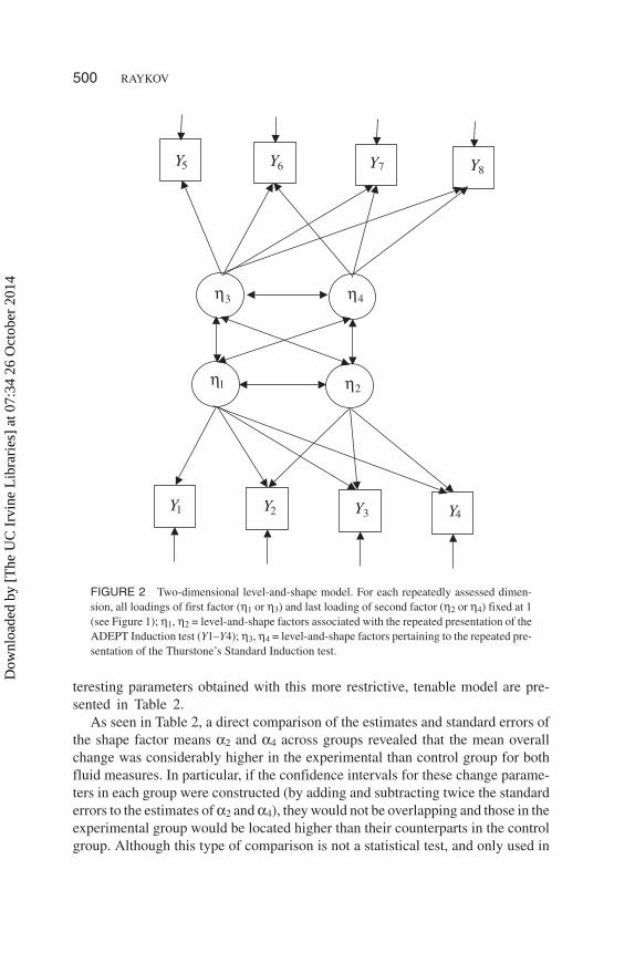
Using all available data from the 335 studied participants on the two repeatedlyadministered induction measures, the ADEPT Induction and Thurstone’s StandardInduction tests, the pattern of simultaneous change over time was investigatedalong the latent dimensions tapped by them and thereby examined the aspects inwhich the experimental and control groups differ. To this end, the level-and-shapemodel was postulated for the four repeated assessments with each of these twofluid tests, and related their level and shape factors across longitudinally followeddimensions. This model is depicted in Figure 2; next this model and a restricted(nested) version of it were fit using the FIML method.

We commence with the variant of the model in Figure 2 that imposes nocross-group constraints and assumes time-invariant impact of error on recordedtest performance (equal error variances across the four assessment occasions).This model is fit to the mean structure of the eight observed variables involved(four assessments with the ADEPT Induction and four with Thurstone’s StandardInduction test). The relevant covariance matrices and means for the FIML proce-dure to be initiated are provided in Table 1 (cf. du Toit & du Toit, 2001).

This starting model is found to be associated with the following acceptable fitindexes: chi-square value, χ2FIML(48) = 68.37, p = .028; and a root mean squareerror of approximation (RMSEA) = .050. Because the random assignment ofparticipants to groups occurred after pretest, no group differences in parameterspertaining to initial measurement were expected, such as initial status (level) fac-tor mean and variance as well as covariance of the two level factors pertaining tothe pair of repeated fluid tests, and the two pretest error variances. Indeed, re-stricting these seven parameters for group invariance yields a minor increase inthe chi-square value up to χ2FIML(55) = 76.78, p = .028; RMSEA = .049, whichalso are tenable fit indexes. Because the difference in the chi-square values forthese two nested models is nonsignificant, namely ∆χ2FIML = 8.41 for differencein degrees of freedom being ∆df = 7 (associated p > .05), there is no evidence inthe data for group differences in initial ability means, variances and covariance,as well as error variances. The estimates with standard errors of substantively in-

LONGITUDINAL SEM ANALYSIS USING FIML 499

Dow

nloa

ded

by [

The

UC

Irv

ine

Lib

rari

es]

at 0

7:34

26

Oct

ober

201

4

teresting parameters obtained with this more restrictive, tenable model are pre-sented in Table 2.

As seen in Table 2, a direct comparison of the estimates and standard errors ofthe shape factor means α2 and α4 across groups revealed that the mean overallchange was considerably higher in the experimental than control group for bothfluid measures. In particular, if the confidence intervals for these change parame-ters in each group were constructed (by adding and subtracting twice the standarderrors to the estimates of α2 and α4), they would not be overlapping and those in theexperimental group would be located higher than their counterparts in the controlgroup. Although this type of comparison is not a statistical test, and only used in

500 RAYKOV

FIGURE 2 Two-dimensional level-and-shape model. For each repeatedly assessed dimen-sion, all loadings of first factor (η1 or η3) and last loading of second factor (η2 or η4) fixed at 1(see Figure 1); η1, η2 = level-and-shape factors associated with the repeated presentation of theADEPT Induction test (Y1–Y4); η3, η4 = level-and-shape factors pertaining to the repeated pre-sentation of the Thurstone’s Standard Induction test.

Dow

nloa

ded

by [

The

UC

Irv

ine

Lib

rari

es]

at 0

7:34

26

Oct

ober

201

4

501

TABLE 1Covariance Matrix and Means for the Four Repeated Assessments

With the Two Induction Measures

Variable AI1 AI2 AI3 AI4 TI1 TI2 TI3 TI4

Experimental groupa 101.0497.04 150.9199.89 140.61 155.03

100.14 137.92 140.86 156.04102.14 126.25 127.86 125.75 148.31103.68 151.06 151.24 146.95 139.61 177.80103.01 147.42 152.51 146.83 137.14 168.95 180.5799.33 144.35 147.67 148.16 134.42 165.19 164.10 174.19

Means 20.86 34.03 35.57 33.32 25.65 36.93 38.05 36.34Control groupb 108.20

112.85 165.03114.21 155.66 170.31111.75 160.25 162.58 178.68112.93 148.39 153.27 156.79 172.08125.92 168.21 174.16 174.76 178.76 218.70123.98 168.65 173.83 177.51 175.97 205.61 220.06126.94 172.76 181.44 186.47 182.48 210.07 211.39 231.10

Means 20.53 28.36 30.54 29.88 26.23 30.72 32.59 32.81

Note. N = sample size (total number of participants, including those with missing values).Covariance matrix and means estimated with the Expectation/Maximization algorithm and used to ini-tiate the full-information maximum likelihood estimation procedure (du Toit & du Toit, 2001).

aN = 219. bN = 116.

TABLE 2Estimates and Standard Errors for Free Factor Loadings, Means,

and Error Variances Associated With the Nested Model (see Figure 2)

Experimental Group Control Group

Parameter Estimate SE Parameter Estimate SE

λ22 1.05 .03 .82 .05λ32 1.16 .03 1.02 .05λ64 1.05 .03 .70 .06λ74 1.14 .03 .96 .06θ11 13.30 .80 13.30 .80θ55 12.19 .73 12.19 .73α1 20.73 .56 20.73 .56α2 12.74 .48 9.20 .61α3 25.84 .68 25.84 .68α4 10.73 .49 6.65 .59

Note. LISREL notation (Jöreskog & Sörbom, 1996) used for denoting model parameters (λs =factor loadings, θs = error variances, time-invariant within repeated measure; αs= factor means).

Dow

nloa

ded

by [

The

UC

Irv

ine

Lib

rari

es]

at 0

7:34

26

Oct

ober

201

4

this section for illustrative and descriptive purposes, it suggests markedly morepronounced overall mean change in the experimental group. Comparing thenacross groups the two free factor loadings of the shape factor per repeatedly admin-istered measure (viz. the parameters λ22 and λ32, and λ64 and λ74), and similarly us-ing their confidence intervals, we see that the experimental group is associatedwith notably larger such loadings. By definition these parameters have the units ofgroup-specific change, which as indicated earlier shows some difference acrossthe groups, and hence their group comparison is meaningful only if considered asindicating pattern of temporal change rather than in an absolute sense. With this inmind, the cross-group comparison of the estimates and confidence intervals for λ22

and λ64 indicates that in the experimental group a notably higher multiple of over-all mean change occurred between pretest and first posttest on both fluid measuresthan in the control group. Similarly, this comparison of estimates and intervals forλ32 and λ74 suggests that with respect to each of the two fluid measures the experi-mental participants exhibited a larger multiple of mean overall change betweenpretest and second posttest. Given that the last loading of the shape factor is 1 onboth tests and groups, a comparison of the estimate and confidence interval of theadjacent loading λ32 with 1 and then of λ74 with 1 reveals that whereas experimen-tal participants showed noticeable decline in mean performance on either fluidmeasure at final posttest, control elderly demonstrated a stable level of perfor-mance at last assessment relative to second posttest. (It is stressed that the meanoverall change in the experimental group was found earlier to be markedly higheron both repeatedly presented fluid measures.) Last but not least, because the firstposttest loadings, λ22 and λ64, are significantly larger than 0, the value of the shapefactor loading at pretest, there was also improvement in mean performance relativeto baseline on both repeated tests in either group.

In summary, the FIML analyses of all available data on the ADEPT Inductionand Thurstone’s Standard Induction tests suggested that the experimental groupexhibited more pronounced improvement in mean performance over the study pe-riod, thereby showing a more salient profile of early improvement than the controlgroup and some decline at delayed posttest (final assessment), whereas the controlgroup maintained a stable level of mean performance after an initial improvementon both fluid measures that remained inferior to that in the experimental groupacross all posttests.

CONCLUSION

This article provided a didactic discussion and empirical illustration of a relativelyrecently developed method of dealing with missing data, the FIML, within theframework of CSM. The approach holds special promise for longitudinal studies

502 RAYKOV

Dow

nloa

ded

by [

The

UC

Irv

ine

Lib

rari

es]

at 0

7:34

26

Oct

ober

201

4

where missing data are the rule rather than the exception. The procedure offers tothe social, behavioral, or educational researcher the opportunity to obtain esti-mates with desirable properties while taking into account all available data from allstudied participants when its assumptions are fulfilled. Although it is still early togive a more comprehensive assessment of the qualities of this modeling approachwhen its assumptions are violated, and particularly that of data missing at random,some recent investigations point to a considerable degree of robustness against upto mild deviations from them (e.g., Collins et al., 2001; Enders, 2001; Schafer &Graham, 2002). Further research is needed into this robustness issue, yet based onthe currently available evidence it is appropriate to recommend the FIML methodas a possible avenue of dealing with the problem of missing data that is so preva-lent in social and behavioral research, and in particular in longitudinal investiga-tions that show increasing popularity over the past several decades across these sci-ences.

ACKNOWLEDGMENTS

This research was conducted during a visit to the Research Institute on Addictions,State University of New York at Buffalo. I am grateful to J. J. McArdle for valuablediscussions on the level-and-shape model; to J. Arbuckle and S. H. C. du Toit forvaluable discussions on FIML; and to P. B. Baltes, F. Dittmann-Kohli, and R.Kliegl for permission to use data from their project “Aging and Fluid Intelligence.”

REFERENCES

Arbuckle, J. L. (1996). Full information estimation in the presence of incomplete data. In G. A.Marcoulides & R. E. Schumacker (Eds.), Advanced structural equation modeling techniques (pp.243–277). Mahwah, NJ: Lawrence Erlbaum Associates, Inc.

Arbuckle, J. L., & Wothke, W. (1999). AMOS 4 user’s guide. Chicago: SmallWaters.Baltes, P. B., Dittmann-Kohli, F., & Kliegl, R. (1986). Reserve capacity of the elderly in aging-sensitive

tasks of fluid intelligence: Replication and extension. Psychology and Aging, 1, 172–177.Bentler, P. M. (2004). EQS structural equation program manual. Encino, CA: Multivariate Software.Collins, L., Schafer, J. L., & Kam, C.-M. (2001). A comparison of inclusive and restrictive strategies in

modern missing data procedures. Psychological Methods, 6, 330–351.Duncan, T., Duncan, S., Striker, L., Li, F., & Alpert (1999). Introduction to the latent growth curve

methodology. Mahwah, NJ: Lawrence Erlbaum Associates, Inc.du Toit, M., & du Toit, S. H. C. (2001). Interactive LISREL: User’s guide. Chicago: Scientific Software

International.Enders, C. K. (2001). A primer on maximum likelihood algorithms available for use with missing data.

Structural Equation Modeling, 8, 128–141.

LONGITUDINAL SEM ANALYSIS USING FIML 503

Dow

nloa

ded

by [

The

UC

Irv

ine

Lib

rari

es]

at 0

7:34

26

Oct

ober

201

4

Horn, J. L. (1982). The aging of human abilities. In B. B. Wolman (Ed.), Handbook of developmentalpsychology (pp. 847–870). New York: McGraw-Hill.

Johnson, R. A., & Wichern, D. W. (2002). Applied multivariate statistical analysis. New York: PrenticeHall.

Jöreskog, K. G., & Sörbom, D. (1996). LISREL8: User’s reference guide. Chicago: Scientific SoftwareInternational.

Maxwell, S. W., & Delany, H. (1990). Analysis of data from experimental studies: A model comparisonapproach. Mahwah, NJ: Lawrence Erlbaum Associates, Inc.

McArdle, J. J., & Anderson, E. (1990). Latent variable growth models for research on aging. In J. E.Birren and K. W. Schaie (Eds.), Handbook of the psychology of aging (2nd ed.) (pp.21–44). NewYork: Academic Press..

Meredith, W., & Tisak, J. (1990). Latent curve analysis. Psychometrika, 55, 175–187.Muthén, B., & Muthén, L. K. (2004). Mplus user’s guide. Los Angeles: Muthén & Muthén.Neale, M. C. (1997). Mx: User’s reference guide. Richmond: Virginia Commonwealth University.Nesselroade, J. R., & Baltes, P. B. (1979). Longitudinal research in the study of behavior and develop-

ment. New York: Academic.Raykov, T., & Marcoulides, G. A. (2000). A first course in structural equation modeling. Mahwah, NJ:

Erlbaum.Schafer, J. L., & Graham, J. W. (2002). Missing data: Our view of the state of the art. Psychological

Methods, 7, 147–177.Sinharay, S., Stern, H. S., & Russell, D. (2001). The use of multiple imputation for the analysis of miss-

ing data. Psychological Methods, 6, 317–329.

APPENDIXLISREL INPUT FILE FOR THE LEVEL-AND-SHAPE

MODEL WITH MISSING DATA

FITTING A TWO-DIMENSIONAL LEVEL-AND-SHAPE MODEL VIA FIML * EXP.GROUP (SEE MCARDLE & HAMAGAMI, 1996, FOR DETAILS ON THE GENERICLEVEL-AND-SHAPE MODEL)DA NI=11 NO=219 NG=2RA=EXPGRP.PSF ! DATA IN PRELIS SYSTEM FILE FORMAT (SEE NOTE)MO NY=8 NE=4 PS=SY,FR AL=FRVA 1 LY 1 1 LY 2 1 LY 3 1 LY 4 1 LY 4 2VA 1 LY 5 3 LY 6 3 LY 7 3 LY 8 3 LY 8 4FR LY 2 2 LY 3 2FR LY 6 4 LY 7 4EQ TE(1)-TE(4)EQ TE(5)-TE(8)ST .5 ALL ! DIFFERENT START VALUES MAY BE NEEDED FOR OTHER DATAOU NS* CONTROL GROUPDA NI=11 NO=116RA=CONGRP.PSF ! DATA IN PRELIS SYSTEM FILE FORMAT (SEE NOTE)MO PS=PS LY=PS TE=PS AL=PSEQ TE 1 1 1 TE 1 1EQ TE 1 5 5 TE 5 5EQ AL(1,1) AL(1)

504 RAYKOV

Dow

nloa

ded

by [

The

UC

Irv

ine

Lib

rari

es]

at 0

7:34

26

Oct

ober

201

4

EQ AL(1,3) AL(3)EQ PS 1 3 1 PS 3 1EQ PS 1 1 1 PS 1 1EQ PS 1 3 3 PS 3 3OU

Note. Uniform symbol used in both data files, EXPGRP.PSF and CONGRP.PSF, todenote missing value (e.g., –999), which is not utilized originally to designate a le-gitimate, nonmissing value; raw data files provided in “PRELIS system file” for-mat (du Toit & du Toit, 2001). On reading these files and finding a missing valuesymbol, LISREL automatically invokes the FIML procedure. (The chi-squarevalue produced evaluates the difference in fit between the fitted and saturated mod-els; e.g., Arbuckle, 1996).

LONGITUDINAL SEM ANALYSIS USING FIML 505

Dow

nloa

ded

by [

The

UC

Irv

ine

Lib

rari

es]

at 0

7:34

26

Oct

ober

201

4