analysis of leading edge flow characteristics in a mixed
TRANSCRIPT
1
Analysis of leading edge flow characteristics in a mixed flow turbine under pulsating flows Samuel P. Lee, Martyn L. Jupp, Simon M. Barrans and Ambrose K. Nickson
Abstract
Current trends in the automotive industry towards engine downsizing means turbocharging now plays a vital role in engine performance. A turbocharger increases charge air density using a turbine to extract waste energy from the exhaust gas to drive a compressor. Most turbocharger applications employ a radial inflow turbine. However, to ensure radial stacking of the blade fibers and avoid excessive blade stresses, the inlet blade angle must remain at zero degrees, creating large incidence angles. Alternately, mixed flow turbines can offer non-zero blade angles while maintaining radial stacking of the blade fibers and reducing leading edge separation at low velocity ratios. Furthermore, the physical blade cone angle introduced reduces the blade mass at the rotor outer diameter reducing rotor inertia and improving turbine transient response. The current paper investigates the performance of a mixed flow turbine under a range of pulsating inlet flow conditions. A significant variation in incidence across the LE span was observed within the pulse, where the distribution of incidence over the LE span was also found to change over the duration of the pulse. Analysis of the secondary flow structures developing within the volute shows the non-uniform flow distribution at the volute outlet is the result of the Dean effect in the housing passage. In-depth analysis of the mixed flow effect is also included, showing that poor axial flow turning ahead of the rotor was evident, particularly at the hub, resulting in modest blade angles. This work shows that the complex secondary flow structures that develop in the turbine volute are heavily influenced by the inlet pulsating flow. In turn, this significantly impacts the rotor inlet conditions and rotor losses. Keywords Mixed flow turbine, secondary flows, computational fluid dynamics Introduction
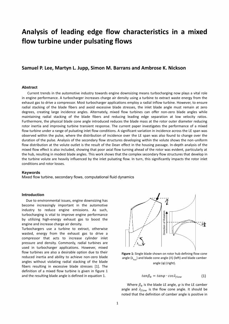
Due to environmental issues, engine downsizing has become increasingly important in the automotive industry to reduce engine emissions. As such, turbocharging is vital to improve engine performance by utilizing high-energy exhaust gas to boost the engine and increase charge air density. Turbochargers use a turbine to extract, otherwise wasted, energy from the exhaust gas to drive a compressor that acts to increase cylinder inlet pressure and density. Commonly, radial turbines are used in turbocharger applications. However, mixed flow turbines are also a desirable option due to their reduced inertia and ability to achieve non-zero blade angles without violating radial stacking of the blade fibers resulting in excessive blade stresses [1]. The definition of a mixed flow turbine is given in figure 1 and the resulting blade angle is defined in equation 1.
Figure 1: Single blade shown on rotor hub defining flow cone angle (λ
flow) and blade cone angle (Λ) (left) and blade camber
angle (φ) (right).
𝑡𝑎𝑛𝛽𝐵 = 𝑡𝑎𝑛𝜑 ∙ 𝑐𝑜𝑠𝜆𝑓𝑙𝑜𝑤 (1)
Where 𝛽𝐵 is the blade LE angle, 𝜑 is the LE camber angle and 𝜆𝑓𝑙𝑜𝑤 is the flow cone angle. It should be
noted that the definition of camber angle is positive in
Λ
λflow
φ
Direction o
f R
ota
tio
n
rota
tio
n

2
the direction of wheel rotation, in figure 1 the wheel contains negative camber, giving rise to a negative blade angle, effectively a swept back configuration. The ability to manipulate the blade LE angle is particularly desirable. A turbocharger turbine operates under highly unsteady pulsating flow conditions due to the nature of the reciprocating engine. Hence, the rotor inlet flows vary significantly as demonstrated in Figure 2 where C represents the absolute flow component, W the relative flow component, U the LE blade velocity and 𝛽 the resulting flow angle. In figure 2 the rotor blade is included to clarity. In this case the radial stacked blade with zero-blade angle (𝛽𝐵) is shown in black and the equivalent mixed flow turbine blade, which is effectively swept back, is shown by the dashed red line, where the blade angle is defined as negative when opposite to the direction of wheel rotation. The resulting LE incidence is calculated from equation 2.
𝑖𝐿𝐸 = 𝛽 + 𝛽𝐵 (2)
The maximum energy in the exhaust pulse is
available at the peak pressure ratio running point which corresponds to the minimum velocity ratio (𝑈/𝑐𝑠) which is defined as the ratio of blade LE velocity to the velocity equivalent of an isentropic enthalpy drop over the turbine and the most positive flow relative angles [2]. Therefore, the non-zero blade angle introduced by the mixed flow effect can reduce loss associated with extreme flow angles and improve efficiency at low velocity ratio, high energy running points within the pulse.
Figure 2: Rotor inlet velocity triangles under pulsating flow.
The unsteady environment created due to the inlet pulsations introduces a significant challenge for designers to ensure the turbine can operate effectively over a wide operating range. The operation of mixed flow turbines under such flows has been assessed by numerous authors [3-5]. Understanding the performance implication of such flows is essential to
improve future designs. As the rotor is fed by the volute which directs and accelerates the flow in to the rotor, the volute design can significantly impact stage performance.
Karamanis et al. [4] completed an experimental study using Laser Doppler Anemometry LDA to investigate the LE and trailing edge (TE) flow components of a mixed flow turbine. The authors obtained distributions of the velocity components over the rotor LE span at two steady state running points. The steady state velocity distributions showed complex flow patterns at the LE, however, a lack of knowledge of the volute flow physics enabled only limited conclusions to be drawn. It was however clear that the rotor was fed with highly non-uniform flow. Furthermore, under pulsating flow the velocity measurements were limited to only the LE mid span and therefore the flow distribution over the span was not investigated.
Rajoo and Martinez-Botas [1] concluded that the poorly guided flow into the rotor found in their investigation and that shown in the computational work by Palfreyman and Martinez-Botas [6], demonstrates that nozzle-less volutes are not adequate in directing rotor inlet flow. However, due to the added expense of nozzle guide vanes and the potential limitation to the range of operation associated with guide vanes [7], vaneless volutes are still widely used.
The impact of volute cross sectional shape on turbine performance was investigated by Yang et al. [8]. This work showed that the change in housing design resulted in a significant variation in rotor performance due to secondary flows in the volute that also affected stage performance. The authors concluded that a better understanding of the impact of volute flows on rotor performance is required.
The development of volute secondary flows in a circular cross sectioned volute was investigated by Lee et al [9] under both steady state and pulsating flow conditions. The authors found Dean-like vortex development in the volute and a significant variation in volute outflow conditions as a result. However, this study was limited to only one pulse frequency and only the volute absolute flow angles were investigated around the volute circumference.
Recently, Morrison et al [10] investigated the impact of rotor inlet conditions on a mixed flow rotor. The authors analyzed rotor flows and LE incidence angles created over a range of inlet conditions. However, the study only focused on steady state work and no volute was included in the study. Instead velocity components at the rotor inlet were applied as boundary conditions and thus removed the impact of the complex flow leaving the volute. However, the authors did show that manipulation of the span-wise variation at the blade LE can lead to performance improvements.
W
U
C
W
Low mass flow High mass flow
+𝛽
−𝛽
U
Radial Blade LE
Mixed Flow Blade LE
𝛽𝐵

3
The current paper investigates the impact of pulsating flows on rotor inlet flow conditions. The analysis includes the flows through the volute passage to better understand the substantial span-wise variation in LE incidence encountered. Furthermore, this computational assessment of the impact of pulse variables aims to provide a better understanding of the environment the rotor is exposed to under realistic engine conditions.
Methodology
Figure 3: Computational domain set-up
The current study uses a computational approach to isolate the impact of various pulse characteristics while ensuring consistency of others. Experimentally achieving the required level of control to manage this comparison is very challenging. In particular, Hakeem et al. [11] stated that independent control of pulse frequency and pulse shape experimentally is extremely difficult.
Figure 3 shows the computational set-up which consists of three domains, the volute, the rotor and the outlet. In this case a mixed flow rotor is used with a simple circular cross sectioned volute design. A full domain specific mesh study was completed, similar to that recommended by Galindo et al. [12], and was extended to include a boundary mesh independence study, further details of the mesh study conducted are available in [13] . The volute and outlet region domains used an unstructured tetrahedral mesh developed in ICEM CFD. The rotor region used a structured hexahedral mesh completed in ANSYS TurboGrid. All CFD simulations were completed in CFX 17 using the Shear Stress Transport (SST) turbulence model, with the frozen rotor approach to account for the turbine rotation as used by a number of authors [14-16]. Furthermore, Yang et al. [15] used the same computational approach and showed good agreement with experimental results under both steady state and pulsating flows. The only discrepancies between experimental and computational results noted by the authors was the magnitude of the hysteresis loop
formed. This was attributed to the impact of the volute tongue on the flow distribution that is not accurately modelled with the frozen rotor method. Yang et al. [17] compared the frozen rotor and sliding mesh method in detail. The authors found that the circumferential non uniformity in tangential and meridional velocity along rotor torque were well predicted by the frozen rotor method. However, discrepancies between the two methods was observed in a detailed study of the passage secondary flows due to the impact of the volute tongue. It was demonstrated that this discrepancy was the result of the difference in the time scale of the secondary flow development and that of the wheel rotation. Analysis of the secondary flows in the rotor passage away from the volute tongue showed no noticeable differences in flow development.
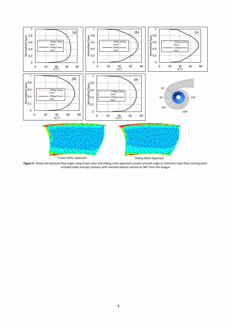
The geometry studied in the current investigation is that of a vaneless mixed flow turbine (no stator guide vanes). Therefore, the only circumferential non-uniformity present was that of the volute tongue. The impact of the frozen rotor approach was assessed, as it was deemed necessary to validate the capability of the frozen rotor approach to predict the volute exit flows. The frozen rotor method was compared with that of the sliding mesh approach under non-pulsating flows at high and low mass flow. The time step size in the sliding mesh simulations was equivalent to 4° of rotor rotation and the results averaged over multiple rotations. In the sliding case the rotor torque fluctuates as each rotor blade passes the volute tongue, while the constant position of the rotor in the frozen rotor approach results in a constant torque. The variation in rotor torque, averaged over multiple rotor rotations between the sliding and frozen rotor approaches was found to be 1.02% and 0.52% in the low and high mass flow cases respectively. Figures 4 and 5 present the span-wise variation of absolute flow angle at the rotor inlet at 5 circumferential locations at both the low and high mass flow running points. In both cases the trends in span-wise variation show good agreement around the rotor circumference with the frozen rotor method only showing a slight over prediction relative to the sliding mesh method. Furthermore figure 4 and 5 also include contour plots of static entropy at 10% chord with velocity vectors over laid at 180° from the volute tongue using both approaches. Both methods show similar flow structures and loss regions further supporting the validity of the frozen rotor approach.
4
Figure 4: Volute exit absolute flow angle using frozen rotor and sliding mesh approach around azimuth angle at minimum mass flow running point.
Included static entropy contours with overlaid velocity vectors at 180° from the tongue.
0
0.2
0.4
0.6
0.8
1
0 20 40 60 80
No
rmal
ized
Sp
an
α (°)
54deg slidingmesh54deg frozenrotor
0
0.2
0.4
0.6
0.8
1
0 20 40 60 80
No
rmal
ized
Sp
an
α (°)
90deg slidingmesh90deg frozenrotor
0
0.2
0.4
0.6
0.8
1
0 20 40 60 80
No
rmal
ized
Sp
an
α (°)
126deg slidingmesh
126deg frozenrotor
0
0.2
0.4
0.6
0.8
1
0 20 40 60 80
No
rmal
ized
Sp
an
α (°)
198deg slidingmesh
198deg frozenrotor
(d)
0
0.2
0.4
0.6
0.8
1
0 20 40 60 80
No
rmal
ized
Sp
an
α (°)
270deg slidingmesh270deg frozenrotor
(e)
54°
90°
126° 198°
270°
Frozen Rotor Approach Sliding Mesh Approach
(a) (b) (c)

5
Figure 5: Volute exit absolute flow angle using frozen rotor and sliding mesh approach around azimuth angle at maximum mass flow
running point. Included static entropy contours with overlaid velocity vectors at 180° from the tongue.
Computational Validation
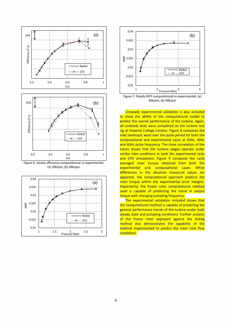
The computational approach used in the current work was further validated against gas stand tests to assess the accuracy of the computational fluid dynamics (CFD) method. This was done at two turbine speeds of 30krpm and 48krpm to assess the accuracy of the predictions over a range of turbine operation. The aim of the validation was to assess the ability of the computational model to predict the performance trends of the mixed flow turbine. Figures 6(a) and 6(b) present the validation of efficiency and figures 7(a) and 7(b) the mass flow parameter (MFP).
All experimental tests were conducted on the cold flow test rig at Imperial College London. Hence the low turbine rotational speeds are the result of the reduced inlet temperature of approximately 320K. The CFD was run to the same cold flow conditions for performance comparisons. Details of the test facilities are available in [8] and [18].
The predicted turbine MFP shows good agreement with the experimental values with only small discrepancies occurring at the highest tested turbine rotational speed. The turbine efficiency characteristics are also well predicted by the CFD model over the majority of the performance maps. However, at the
high velocity ratio running points, where the flow is more unstable, the CFD under predicts the experimentally measured values. At these operating points the errors in the experimental values also increase due to the relative errors in mass flow and pressure measurements increasing.
Despite the variations from the absolute measured efficiency, the characteristics of turbine performance are effectively captured by the CFD model. As stated by [19], CFD calculations are accepted to be better at predicting trends rather than absolute values. Therefore, replication of the turbine performance trends provides a level of confidence in the computational approach used throughout this study.
0
0.2
0.4
0.6
0.8
1
0 20 40 60 80
No
rmal
ized
Sp
an
α (°)
54deg slidingmesh54deg frozenrotor
0
0.2
0.4
0.6
0.8
1
0 20 40 60 80
No
rmal
ized
Sp
an
α (°)
90deg slidingmesh90deg frozenrotor
0
0.2
0.4
0.6
0.8
1
0 20 40 60 80
No
rmal
ized
Sp
an
α (°)
126deg slidingmesh126deg frozenrotor
0
0.2
0.4
0.6
0.8
1
0 20 40 60 80
No
rmal
ized
Sp
an
α (°)
198degsliding mesh
198degfrozen rotor
0
0.2
0.4
0.6
0.8
1
0 20 40 60 80
No
rmal
ized
Sp
an
α (°)
270deg slidingmesh270deg frozenrotor
54°
90°
126° 198°
270°
(a) (b) (c)
(d) (e)
Frozen Rotor Approach Sliding Mesh Approach
6
Figure 6: steady efficiency computational vs experimental.
(a) 30krpm, (b) 48krpm.
Figure 7: Steady MFP computational vs experimental. (a)
30krpm, (b) 48krpm
Unsteady experimental validation is also included
to show the ability of the computational model to predict the overall performance of the turbine. Again, all unsteady tests were completed on the turbine test rig at Imperial College London. Figure 8 compares the inlet isentropic work over the pulse period for both the computational and experimental cases at 20Hz, 40Hz and 60Hz pulse frequency. The close correlation of the traces shows that the turbine stages operate under similar inlet conditions in both the experimental tests and CFD simulations. Figure 9 compares the cycle averaged rotor torque obtained from both the experimental and computational cases. While differences in the absolute measured values are apparent, the computational approach predicts the rotor torque within the experimental error margins. Importantly, the frozen rotor computational method used is capable of predicting the trend in output torque with changing pulsating frequency.
The experimental validation included shows that the computational method is capable of predicting the general performance trends of the turbine under both steady state and pulsating conditions. Further analysis of the frozen rotor approach against the sliding method also demonstrates the capability of the method implemented to predict the rotor inlet flow conditions.
0.4
0.5
0.6
0.7
0.8
0.9
0.2 0.4 0.6 0.8 1
Effi
cien
cy (
T-s)
U/c
Radial
CFD
(a)10%
0.4
0.5
0.6
0.7
0.8
0.9
0.2 0.4 0.6 0.8 1
Effi
cien
cy (
T-s)
U/c
Radial
CFD
(b)10%
0.01
0.015
0.02
0.025
0.03
0.035
0.04
1 1.5 2 2.5 3
MR
P
Pressure Ratio
Radial
CFD
(a)
0.01
0.015
0.02
0.025
0.03
0.035
0.04
1 2 3 4
MR
P
Pressure Ratio
RadialCFD
(b)

7
Figure 8: Unsteady Isentropic work pulse experimental and CFD
Figure 9: Unsteady cycle averaged torque measurements
experimental and CFD
Operating Conditions
The impact of the inlet pulse was investigated at three pulse frequencies (20Hz, 40Hz and 60Hz), three pulse loads, �̇�𝐿𝑜𝑎𝑑, (73%, 100% and 127%) and four pulsation numbers, �̇�𝑛𝑜., (0.5, 0.75, 1 and 1.25). The pulse load and pulsation number are defined in equations 3 and 4 respectively –
�̇�𝐿𝑜𝑎𝑑 = ∫�̇�
𝑇
𝑇
0
𝑑𝑡 (3)
�̇�𝑛𝑜. =
�̇�𝑚𝑎𝑥 − �̇�𝑚𝑖𝑛
�̇�𝐿𝑜𝑎𝑑
(4)
Where �̇� is mass flow rate, 𝑇 is the pulse duration �̇�𝑚𝑎𝑥 is the maximum pulse mass flow rate and �̇�𝑚𝑖𝑛 is the minimum pulse mass flow rate.
The resulting pulses implemented in the study are presented in Figures 10 and 11. The magnitude of the
temperature pulse remained constant throughout the study but the pulse frequency was changed to match the frequency of the corresponding inlet mass flow pulse.
The three pulse frequencies were tested at a pulsation number of 1 and a pulse load of 100%. The three pulse loads implemented were investigated at 40Hz frequency and a pulsation number of 0.5 further increases in the pulsation number would have led to low mass flows, flow reversal and therefore convergence issues. The four pulsation numbers tested were analyzed at 40Hz frequency and a pulse load of 100%.
Figure 10: Inlet mass flow and total temperature pulses at
20Hz, 40Hz and 60Hz frequencies
Figure 11: Inlet mass flow pulses at 40 Hz Left - low, medium
and high load. Right – 0.5, 0.75, 1 and 1.25 inlet pulsation number pulses.
The turbine rotor used in this investigation, shown in figure 12, is a production mixed flow wheel for commercial applications. This particular wheel contains a camber angle varying from approximately -27° at the hub to 13° at the shroud tip and a blade cone angle of 20°. Thus, there is a variation in blade angle from hub to shroud. As is the nature of mixed flow turbines the tip speed varies from hub to shroud. This variation, due to the conservation of angular momentum, has been shown to result in a variation in LE incidence [10]. Furthermore, the LE incidence in mixed flow turbines is heavily dependent on the axial flow component at the LE of the rotor and the distribution of flow angle at the volute exit. As the blade camber and flow cone angles can be used to manipulate the LE blade angle a thorough understanding of the impact that pulsating flow has on rotor incidence over the LE span is necessary for further performance optimization.
0
2
4
6
8
10
12
14
16
0 0.01 0.02 0.03 0.04 0.05
Isen
tro
pic
Wo
rk (
kW)
Time (s)60Hz CFD 60Hz EXP40Hz CFD 40Hz EXP
0.7 0
0.7 5
0.8 0
0.8 5
0.9 0
0.9 5
1.0 0
0 20 40 60
Ro
tor
Torq
ue
(Nm
)
Pulse Frequency (Hz)
EXP CFD
0.050
0.0 5
0.1
0.1 5
0.2
0.2 5
0.3
0 0.025 0.05
Mas
s Fl
ow
Kg/
s
Time (s)
20Hz40Hz60Hz
700
800
900
1000
1100
0 0.025 0.05
Tota
l Tem
per
atu
re (
K)
Time (s)
20Hz
40Hz
60Hz
0.1
0
0.0 5
0.1
0.1 5
0.2
0.2 5
0.3
0 0.01 0.02
Mas
s Fl
ow
(K
g/s)
Time (s)
Low
Mid
High0
0.0 5
0.1
0.1 5
0.2
0.2 5
0.3
0 0.01 0.02
Mas
s Fl
ow
Kg/
s)
Time (s)
0.5
0.75
1
1.25
0.1 0.1

8
Figure 12: Mixed flow rotor design
Results and Discussion – Impact of Pulse Frequency
Figure 13 presents the mass flow at the stage inlet and rotor inlet against normalized time for 20Hz, 40Hz and 60Hz pulse frequencies. The mass flow range measured at the rotor inlet shows a gradual reduction with increasing frequency. This is the result of increased mass flow damping through the volute at higher frequencies. Increasing frequency resulted in flattening of the pulse peak leading to a plateau at peak mass flow in the 60Hz case spanning approximately 30% of the pulse.
Figure 13: Stage inlet and rotor inlet mass flow at 20Hz, 40Hz
and 60Hz pulse frequencies
The turbine Mass Flow Parameter (MFP) hysteresis is presented in figure 14 for each of the tested frequencies. With increasing frequency, the deviation in MFP from the steady state results increases and the range of pressure ratios experienced reduces from 1.25-2.35 at 20Hz, to 1.29-2.31 at 40Hz and 1.38-2.23 at 60Hz. The hysteresis formed around the steady state performance line greatly increases with pulsating frequency. Notably, in the 60Hz case the peak MFP is achieved in the middle of the pressure ratio range and begins to reduce while the pressure ratio continues to increase. This effect can be attributed to the reflected pressure wave traveling back through the volute to the measurement plane.
Figure 14: MFP vs pressure ratio for steady state, 20Hz, 40Hz
and 60Hz inlet conditions
The resulting rotor torque, presented in figure 15, resembles the corresponding rotor inlet mass flow at each frequency. With increasing frequency, the torque range reduces and the shape of the curve towards the peak sees a change in shape resulting in a reduction in the gradients in that region.
The rotor efficiency from the three pulse frequencies presented in figure 16 shows that the maximum velocity ratio experienced under the 20Hz pulse is the greatest reaching a peak U/cs of 0.99 while the 40Hz and 60Hz cases reach U/cs’s of 0.93 and 0.83 respectively. The minimum velocity ratio achieved in all cases was approximately 0.45. While the range of rotor operation is significantly reduced with increasing frequency, the efficiency curve at a given U/cs
converges for all frequencies and as the U/cs increases the hysteresis formed reduces.
Figure 15: Resulting rotor torque at 20Hz, 40Hz and 60Hz
pulse frequencies
0.01
0.015
0.02
0.025
0.03
0.035
0.04
1.2 1.4 1.6 1.8 2 2.2 2.4
MFP
Pressure Ratio
20Hz
40Hz
60Hz
Steady State
0
0.0 5
0.1
0.1 5
0.2
0.2 5
0.3
0 0.2 0.4 0.6 0.8 1
Mas
s Fl
ow
(K
g/s)
Normalized Time
20Hz
40Hz
60Hz
Inlet Mass Flow
0.05
0
0.5
1
1.5
2
2.5
3
3.5
4
4.5
0 0.2 0.4 0.6 0.8 1
Ro
tor
Torq
ue
(Nm
)
Normalized time
20Hz
40Hz
60Hz
1
9
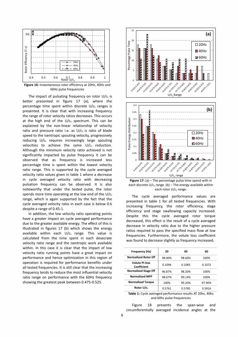
Figure 16: Instantaneous rotor efficiency at 20Hz, 40Hz and
60Hz pulse frequencies
The impact of pulsating frequency on rotor U/cs is better presented in figure 17 (a), where the percentage time spent within discrete U/cs ranges is presented. It is clear that with increasing frequency the range of rotor velocity ratios decreases. This occurs at the high end of the U/cs spectrum. This can be explained by the non-linear relationship of velocity ratio and pressure ratio i.e. as U/cs is ratio of blade speed to the isentropic spouting velocity, progressively reducing U/cs requires increasingly large spouting velocities to achieve the same U/cs reduction. Although the minimum velocity ratio achieved is not significantly impacted by pulse frequency it can be observed that as frequency is increased less percentage time is spent within the lowest velocity ratio range. This is supported by the cycle averaged velocity ratio values given in table 1 where a decrease in cycle averaged velocity ratio with decreasing pulsation frequency can be observed. It is also noteworthy that under the tested pulse, the rotor spends more time operating at the low end of the U/cs range, which is again supported by the fact that the cycle averaged velocity ratio in each case is below 0.6 despite a range of 0.45-1.
In addition, the low velocity ratio operating points have a greater impact on cycle averaged performance due to the greater available energy. The effect of this is illustrated in figures 17 (b) which shows the energy available within each U/cs range. This value is calculated from the time spent in each desecrate velocity ratio range and the isentropic work available within. In this case it is clear that the impact of low velocity ratio running points have a great impact on performance and hence optimization in this region of operation is required for performance benefits under all tested frequencies. It is still clear that the increasing frequency tends to reduce the most influential velocity ratio range on performance with the 60Hz frequency showing the greatest peak between 0.475-0.525.
Figure 17: (a) – The percentage pulse time spend with in
each discrete U/cs range. (b) – The energy available within each rotor U/cs range.
The cycle averaged performance values are presented in table 1 for all tested frequencies. With increasing frequency, the rotor efficiency, stage efficiency and stage swallowing capacity increased. Despite this the cycle averaged rotor torque decreased, this effect is the result of a cycle averaged decrease in velocity ratio due to the higher pressure ratios required to pass the specified mass flow at low frequencies. Furthermore, the volute loss coefficient was found to decrease slightly as frequency increased.
Frequency (Hz) 20 40 60
Normalized Rotor Eff 98.00% 98.60% 100%
Volute Pt loss Coefficient
0.1094 0.1083 0.1072
Normalized Stage Eff 96.87% 98.20% 100%
Normalized MFP 98.67% 99.14% 100%
Normalized Torque 100% 99.20% 97.90%
Rotor U/cs 0.5761 0.5785 0.5816
Table 1: Cycle averaged performance results AT 20hz, 40hz and 60hz pulse frequencies
Figure 18 presents the span-wise and circumferentially averaged incidence angles at the
0
5
10
15
20
25
Per
cen
tage
Pu
lse
Tim
e
U/cs Range
20Hz
40Hz
60Hz
0
0.05
0.1
0.15
0.2
0.25
0.3
0.35
0.4
Pu
lse
Ener
gy D
istr
ibu
tio
n
U/cs range
20Hz
40Hz
60Hz
0.4
0.4 5
0.5
0.5 5
0.6
0.6 5
0.7
0.7 5
0.8
0.4 0.5 0.6 0.7 0.8 0.9 1
Ro
tor
Effi
cien
cy (
T-s)
Rotor U/cs
20Hz
40Hz
60Hz
5% (a)
(b)

10
blade LE (𝑖𝐿𝐸) at points in time over the pulse duration. The average blade LE Incidence is calculated from the mass flow averaged velocity components around the rotor LE circumference and the span-wise averaged blade LE camber angle (𝜑) . As frequency is increased the minimum incidence angles achieved reduce in magnitude significantly. Alternately, the maximum incidence angles achieved do not vary significantly with pulse frequency. While the mass flow pulses, shown in figure 13, show a greater variation at the pulse minimum, a significant variation in the peak also exists. However, the LE incidence evidently doesn’t experience the same variation. The increased impact of the mass flow variation on incidence angle at lower angles can be visualized through the velocity triangles as shown in figure 2. At low mass flow operation (negative incidence) a reduction in the velocity component C, will have a greater impact of the resulting relative flow angle than the same absolute increase would have at maximum mass flow operation. Hence, how the incidence angle range change with frequency does not necessarily follow the same trend as the mass flow.
Figure 18: Mass flow averaged leading edge incidence angle throughout pulse at 20Hz, 40Hz and 60Hz pulse frequencies
As previously discussed, the incidence angle in a mixed flow turbine is dependent on the volute exit flow angles and the blade angle achieved. The mixed flow rotor used in this case has varying LE camber and therefore the blade angle from hub to shroud is not constant. However, for this to be implemented successfully it is necessary to understand the span-wise variation in flow conditions under pulsating conditions.
Firstly, the span-wise variation in flow cone angle is assessed. This is presented in figure 19 under 40Hz pulse frequency at three points in time over the pulse duration: minimum incidence, -10° LE incidence during the emptying phase of the pulse) and maximum incidence. These three points are extracted from figure 18. In all cases the flow cone angle is greater than the 70° required for flow to enter the rotor normal to the LE, indicating a lack of flow turning ahead of the rotor. This is particularly evident at the minimum incidence
running point where the flow cone angle remains above 80° over 85% of the LE. However, as this running point corresponds to highly negative incidence, the addition of the mixed flow effect is not beneficial at this point in the pulse. At the -10° and maximum incidence running points, the flow cone angle achieved is significantly smaller. Poor flow turning at the hub is particularly evident, and the variation from hub to shroud is substantial in both cases.
Figure 19: Leading edge Flow cone angle at three points over
the blade span during the 40Hz inlet pulse
The resulting blade angles achieved from the combination of the LE camber angle and flow cone angle are presented in figures 20(a)-(b) for the 20Hz, 40Hz and 60Hz cases respectively. In all cases, a significant variation in blade LE angle is observed over the blade span. The maximum magnitude achieved is only -4.9° at the maximum incidence running point for all tested frequencies. In all cases the blade angle becomes increasingly positive towards the shroud as a result of the positive blade camber present in this region. While the blade angle at -10° and maximum incidence appear to be independent of pulse frequency, significant variations in the LE blade angle at minimum incidence is apparent. At 20Hz, the blade LE angle reaches a maximum negative magnitude of only -2.5° at 20% span. However, with increasing frequency the deviation of the blade angle at the minimum incidence running point reduces. This effect is the result of the lower mass flow achieved under lower frequency.
-60
-40
-20
0
20
0 0.2 0.4 0.6 0.8 1
LE In
cid
ence
An
gle
(deg
)
Normalized Time
20Hz
40Hz
60Hz
0%
20%
40%
60%
80%
100%
70 75 80 85 90 95LE
Sp
anFlow Cone Angle (deg)
Min Inc
-10 deg
Max Inc
0%
20%
40%
60%
80%
100%
-6 -4 -2 0 2 4 6
LE S
pan
Blade LE angle (deg)
Min Inc
-10 deg
Max Inc
(a)

11
Figure 20: Leading edge blade angle at three points in the
pulse. (a) – 20hz, (b) – 40Hz, (c) – 60Hz
The resulting LE incidence is plotted in figures 21(a)-(c) for the minimum, -10° and maximum incidence running points respectively at all tested pulse frequencies. The variation in incidence over the rotor span is large in all cases. At minimum incidence, the lowest flow angles are achieved at the rotor hub, increasing to a maximum at approximately 20% chord. Incidence reaches a local minimum at center span before increasing again to a maximum at the shroud side. While the distribution of incidence at the LE remains similar for all pulse frequencies, the distribution shifts to a more negative mean as the pulse frequency is reduced. The impact of pulse frequency on the mean incidence was not observed at the maximum LE incidence running point. The velocity ratio at this point corresponds to the minimum velocity ratio and as shown in figure 17 frequency has little impact on U/cs at this end of the range. However, at the minimum incidence running point, which corresponds to the maximum velocity ratio, a notable difference in the values was achieved when pulse frequency was varied.
At -10° incidence, the minimum incidence over the blade span is achieved at the hub and increases to a maximum at around the center of the LE before decreasing again towards the shroud at a more gradual rate. At this operating point, the frequency does not have a significant impact on the distribution of incidence.
At the maximum incidence point, a distribution with a parabolic-like shape is formed at all pulsed
frequencies with the maximum incidence achieved in the center of the LE. Again, for all tested frequencies, the distribution and mean incidence angles are very similar.
The resulting span-wise variation in incidence angle is clearly heavily influenced by inlet pulsations. While [10] noted the impact of varying blade speed at the LE of a mixed flow turbine as a source of incidence variation, this effect is not observed in the current study. This is put down to the fact that the span-wise variation of the velocity components exiting from the volute (which were not accounted for by [10]) has a substantial impact on the blade LE incidence of the current rotor with a mild blade cone angle of only 20°.
Figure 21: Leading edge incidence over the blade span at 20Hz, 40Hz and 60Hz pulse frequencies. (a) – minimum
incidence, (b) -10° incidence, (c) maximum incidence
The variation in relative circumferential velocity with respect to the mean velocity is presented in
0%
20%
40%
60%
80%
100%
-6 -4 -2 0 2 4 6
LE S
pan
Blde LE angle (deg)
Min Inc
-10deg
Max Inc
(b)
0%
20%
40%
60%
80%
100%
-6 -4 -2 0 2 4 6
LE S
pan
Blde LE angle (deg)
Min Inc
-10 deg
Max Inc
(c)
0%
20%
40%
60%
80%
100%
-80 -60 -40 -20 0 20 40
LE S
pan
LE Incidence Angle (deg)
Min Inc 20HzMin Inc 40HzMin Inc 60Hz
(a)
0%
20%
40%
60%
80%
100%
-80 -60 -40 -20 0 20 40
LE S
pan
LE Incidence Angle (deg)
-10deg Inc 20Hz
-10deg Inc 40Hz
-10deg Inc 60Hz
(b)
0%
20%
40%
60%
80%
100%
-80 -60 -40 -20 0 20 40
LE S
pan
LE Incidence Angle (deg)
Max Inc 20Hz
Max Inc 40Hz
Max Inc 60Hz
(a)

12
figure 22 at minimum, -10° and maximum incidence. In all cases the general shape of the distribution represents that of fully developed pipe flow which can be expected due to the flow development within the volute. Towards the hub the circumferential velocity becomes increasingly positive due to the proximity of blade hub surface. Towards the shroud the velocity becomes increasingly negative due to the relative movement of the shroud surface with respect to the passage. The central 60% of the span sees a more constant circumferential velocity distribution but as incidence increase so does the variation over this region.
Figure 22: Variation in circumferential velocity about the
mean velocity at the blade leading edge at 40Hz
Figure 23: Variation in radial velocity about the mean
velocity at the blade leading edge at 40Hz
Figure 23 shows the variation in meridional velocity from the mean over the same three running points as in figure 22. In all cases a local minimum radial velocity
occurs in the center of the LE (excluding that occurring very close to the hub surface) and the velocity increases towards both the hub and shroud. This trend becomes more pronounced with increasing incidence angle as the peak of the inlet pulse is approached.
This behavior is the result of the development of flows within the volute and was discussed previously by Lee et al [9]. Figure 24 shows contours of radial velocity and surface streamlines on six planes around the volute at 40Hz pulse frequency at both the minimum and maximum incidence running points. The position of the six planes are 54°, 72°, 90°, 126°, 198° and 270°.
At the minimum incidence running point in the 72° plane, two pairs of counter rotating vortices form on each side of the volute. The higher vortices rotate clockwise and lower vortices in the counter-clockwise direction. These flow structures develop as a result of the Dean effect, where the high velocity central passage flow with higher inertia is more resistant to radial turning compared with the lower inertia flow adjacent to the volute walls. As a result, the flow near the walls turns radially in more readily than the bulk central flow. The variation in radial velocity across the volute passage exit is the result of this mechanism. In the 90° plane, the vortices no longer exist but a distinct deviation in the streamlines low in the volute can be observed. While the vortex structures do not persist further around the volute a clear variation in radial velocity from the contour plots is visible around the volute passage and is particularly evident at the volute exit.
At the maximum incidence running point, no distinct vortex regions were observed. Despite this, the variation in radial velocity shown in the contour plot is still large. The lack of vortex formation is attributed to the positive pressure gradient pushing the flow into the rotor; this driving force suppresses any potential flow reversal. The same effect explains the rapid breakdown of the vortices at the minimum incidence running point as volute area reduces. Despite the lack of vortices a significant variation in radial velocity over the volute cross section is evident at all plotted positions.
0%
20%
40%
60%
80%
100%
-150 -100 -50 0 50 100 150 200
LE S
pan
Circumfrential Velocity Relative to Spanwise Mean (m/s)
Min Inc 40Hz
-10 deg 40Hz
Max Inc 40Hz
0%
20%
40%
60%
80%
100%
-150 -100 -50 0 50 100 150 200
LE S
pan
Meridonal Velocity Relative to Spanwise Mean (m/s)
Min Inc 40Hz
-10 deg 40Hz
Max Inc 40Hz
13
Figure 24: Stream lines and radial velocity contours at planes around the volute circumference. Left - minimum incidence running point. Right - maximum incidence running point
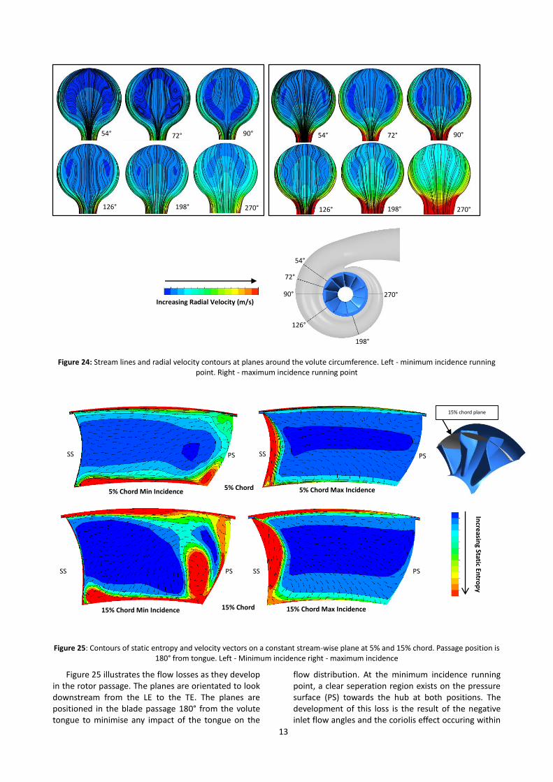
Figure 25: Contours of static entropy and velocity vectors on a constant stream-wise plane at 5% and 15% chord. Passage position is
180° from tongue. Left - Minimum incidence right - maximum incidence
Figure 25 illustrates the flow losses as they develop in the rotor passage. The planes are orientated to look downstream from the LE to the TE. The planes are positioned in the blade passage 180° from the volute tongue to minimise any impact of the tongue on the
flow distribution. At the minimum incidence running point, a clear seperation region exists on the pressure surface (PS) towards the hub at both positions. The development of this loss is the result of the negative inlet flow angles and the coriolis effect occuring within
Increasing Radial Velocity (m/s)
54° 54° 72° 90° 72° 90°
126° 198° 270° 126° 270° 198°
Incre
asing Static En
trop
y
SS SS PS PS
SS SS PS PS
5% Chord Min Incidence
15% Chord
5% Chord Max Incidence
15% Chord Min Incidence 15% Chord Max Incidence
5% Chord
54°
72°
90°
126°
198°
270°
15% chord plane

14
the passage. The loss region initiates close to the hub at the 5% chord position and grows to the 15% chord position. The region also moves away from the PS due to the cross-passage pressure gradient. There are also significant loss regions at the shroud due to the relative movement at the surface.
At the maximum incidence running point, separation from the SS is evident at the blade span centre and reduces towards both the hub and shroud. This compares favourably with the incidence distribution shown in figure 21©. The high entropy region at the shroud is the result of the relative movement of the shroud and the interaction with tip leakage.
The variation in incidence over the LE span at five points around the volute circumference (54°, 90°, 126°, 198° and 270°) are shown in figures 26(a) and (b) for the minimum and maximum incidence points respectively. Incidence was extracted at these positions as they are located midway between the rotor blades (18° from both neighboring LE’s). This is done to minimize the upstream effect on the flow distribution and therefore focus on that produced by the volute. In both cases the variation in the LE incidence over the rotor span was influenced by circumferential positions. At the 54° position, the incidence across the span remains the most consistent in both cases. The greatest variation in incidence is then experienced at 126° from the tongue in both cases. However, this effect makes the flow increasingly negative at the span center in the minimum incidence case and increasingly positive at the span center in the maximum incidence case. Beyond the 126° position the variation reduces in both cases and then remains almost constant at the 198° and 270° positions.
Figure 26: Leading edge incidence around the volute circumference at minimum incidence (a) and maximum incidence (b) during the 40Hz pulse
Impact of Pulse Load
In this study, three mass flow pulse loads (low load – 73%, mid load 100% and high load – 127%) were tested and the resulting MFP is plotted against stage pressure ratio in figure 27. All loads were tested at 40Hz pulse frequency and pulsation number of 1. There is a clear change in the shape of the hysteresis with changing pulse load. Also, the hysteresis increases with load resulting in greater deviation from the steady state results at higher loads. The range of the stage pressure ratio over the pulse also increases with increasing load. This behavior is the result of the increasing inlet mass flow. As the stage approaches the choked condition larger pressure ratios are necessary to achieve further increases in mass flow resulting in a reduction of the MFP range over the pulse and an increase in the pressure ratio range.
Figure 27: MFP vs pressure ratio for steady state, low,
medium and high load at 40Hz pulse frequency
The resulting rotor torque is presented in figure 38. While the pulse frequency had significant impact on the shape of the turbine torque generated over the course of the pulse, the turbine load has little impact on this. Meanwhile the torque mean experiences a distinct shift up with increasing turbine load which is to be expected.
0%
20%
40%
60%
80%
100%
-90 -60 -30 0 30
LE S
pan
LE Incidence (deg)
54 deg90 deg126 deg198 deg270 deg
0%
20%
40%
60%
80%
100%
-90 -60 -30 0 30
LE S
pan
LE Incidence (deg)
54 deg
90 deg
126 deg
198 deg
270 deg
0.0 15
0.0 2
0.0 25
0.0 3
0.0 35
0.0 4
1.1 1.3 1.5 1.7 1.9 2.1 2.3 2.5
MFP
PR
Low
Mid
High
Steady State
0.05

15
The resulting rotor efficiency for each turbine load presented in figure 29 shows that the mean rotor velocity ratio shifts to lower values with an increase in load and that the rotor velocity range significantly reduces. The resulting efficiencies, particularly at low velocity ratios, collapse onto a single line demonstrating the quasi steady performance of the rotor. However, as with varying frequency the hysteresis in performance increases at high velocity ratios.
Figure 28: Rotor torque of the 40Hz pulse at three load
conditions
Figure 29: Instantaneous rotor torque at three load
conditions at the 40Hz pulse frequency
The turbine performance parameters achieved under each load are presented in table 2. In the current case the lowest tested turbine load achieves the greatest rotor and stage efficiencies. While increasing load results in a considerable increase in torque produced, the energy demands required are also much higher. Increased aerodynamic loss associated with the higher pressure running points result in a reduction in efficiency as the turbine performs over a more inefficient range of operation. Alternately it was found that the volute loss coefficient reduces with increasing load.
The resulting rotor LE incidence is plotted in figure 30. Increasing the turbine load increases the mean incidence over the pulse cycle. Furthermore, the range
of incidence decreases significantly as the load is increased which is predominantly the result of changes to the minimum incidence range. Under the maximum load pulse, incidence ranged from -5.1° to 15.6°, at the middle load from -24.1° to 14.8° and under the lowest load pulse from -55.8° to 7.3°. The results show that at higher loads, incidence is less sensitive to mass flow changes.
Figure 30: Leading edge incidence over the 40Hz pulse at
three load conditions
The variation in incidence over the rotor LE span is presented at the minimum incidence in figure 31(a) for the three test pulse loads. At the minimum incidence angle running point the incidence over the span between the three pulse loads exhibits different profiles. At the lowest load, minimum incidence occurs at the hub wall increasing to a maximum at 15% span, then reducing to a local minimum at the center and showing a moderate increase towards the shroud. The middle load results in an almost constant distribution from the 20% span position to the shroud side. This running point of the middle load pulse corresponds to peak rotor efficiency where mean incidence is approximately -20°. The high load point shows the opposite distribution to that observed at low load. The most positive values occur at the center of the blade span and decrease towards both the hub and shroud.
-60
-40
-20
0
20
0 0.2 0.4 0.6 0.8 1
LE In
cid
ence
An
gle
(deg
)
Normalized Time
LowMidHigh
Table 2: Cycle-averaged performance results for three load conditions at 40Hz pulse frequency
Pulse Load Low Mid High
Normalized Rotor Eff 100% 98.14% 92.73%
Volute Pt loss Coefficient
0.1151 0.1114 0.0991
Normalized Stage Eff 100% 98.64% 93.71%
Normalized MFP 81.72% 93.79% 100%
Normalized Torque 36.24% 66.08% 100%
Rotor U/cs 0.6918 0.5842 0.5162
0
0.5
1
1.5
2
2.5
3
3.5
4
4.5
5
0 0.2 0.4 0.6 0.8 1
Ro
tor
Torq
ue
(Nm
)
Normalized Time
Low
Mid
High
0.5
0.4
0.4 5
0.5
0.5 5
0.6
0.6 5
0.7
0.7 5
0.8
0.4 0.5 0.6 0.7 0.8 0.9 1
Ro
tor
Effi
cien
cy
Rotor U/cs
Low
Mid
High
5%

16
Figure 31: Leading edge incidence over the blade span under
three load conditions at 40Hz pulse frequency. (a) – minimum incidence, (b) – maximum incidence
At the maximum incidence running points shown in figure 31(b), incidence over the span shows similar distribution for all three loads. At the lowest tested load, the incidence remains approximately 5° less than that of the middle and high load pulses over the entire span but the distribution shape is similar. The variation between the middle and high load pulses is negligible despite both points having significantly different mass flows. This finding further illustrates that the mean incidence and incidence distribution is approximately constant beyond a certain mass flow value. Impact of Pulsation Number
Four pulsation numbers were tested (0.5, 0.75, 1 and 1.25) at 40Hz frequency and a pulse load of 100%. The resulting stage MFP plots for the four pulses are presented in figure 32. As the pulsation number increases, the MFP hysteresis and stage pressure ratio range increase, however, the shape of the hysteresis loop is similar.
Figure 32: MFP vs pressure ratio for steady state, 50, 75, 100
and 125 pulsation numbers at 40Hz pulse frequency
The resulting rotor torque is plotted in figure 33. The range of rotor torque achieved increases with increasing pulsation number resulting in a significant increase in the rate of change with time. The range of rotor velocity ratio also increases significantly with increasing pulsation number. The energy distribution available over the velocity ratio range is presented in figure 34. As the pulsation number increases the maximum rotor velocity ratio achieved was found to increase significantly, however due to the low energy availability in this region this has negligible impact on cycle averaged performance. The impact on the U/cs at the low end of the range is less distinct, but an increase in available energy at the low velocity ratios can be observed as pulsation number is increased. This is supported by the reduction in cycle averaged velocity ratio as pulsation number increases as shown in table 3.
Figure 33: Rotor torque over the pulse at 50, 75, 100 and 125
pulsation numbers at 40Hz pulsation frequency
0%
20%
40%
60%
80%
100%
-100 -80 -60 -40 -20 0 20 40
LE S
pan
Incidence (deg)
LOW LOADMID LOADHIGH LOAD
(a)
0%
20%
40%
60%
80%
100%
-80 -60 -40 -20 0 20 40
LE S
pan
Incidence (deg)
LOW LOADMID LOADHIGH LOAD
(b)
0.0 1
0.0 15
0.0 2
0.0 25
0.0 3
0.0 35
0.0 4
1 1.2 1.4 1.6 1.8 2 2.2 2.4 2.6
MFP
PR
0.5
0.75
1
1.25
Steady State
0.05
0
0.5
1
1.5
2
2.5
3
3.5
4
4.5
0 0.2 0.4 0.6 0.8 1
Ro
tor
Torq
ue
(Nm
)
Normalised Time
0.50.7511.25
0.5

17
Figure 34: Rotor operating velocity ratio over pulse
Table 3 presents the cycle-averaged performance
for each of the tested pulsation numbers. With increasing pulsation number, the stage and rotor efficiency decreased. This was the result of the increased range of operation causing the turbine to operate at increasingly off design conditions. It was also observed that the volute total pressure loss coefficient decreased with increasing pulsation number. Throughout this study it has been apparent that volute losses reduce when the turbine operates away from the low mass flow running points where secondary flow structures more commonly form as shown in figure 24.
The resulting LE incidence over the pulse cycle is presented figure 35. It can be seen that the peak incidence angle is not significantly impacted by the pulsation number with maximum incidence ranging between 16.71° and 13.36° for the 1.25 and 0.5 pulsation number pulses. However, the pulsation number does have a significant impact on the minimum incidence angle achieved with minimum incidence angles of -24.09°, -37.88°, -52.39° and -62.44° achieved for the 0.5, 0.75, 1 and 1.25 pulsation number pulses respectively. This effect is similar to that experience under the range of tested frequencies. The reason for this is that to further increase the incidence to positive values, the absolute velocity (C) must exponentially increase. Alternately, to reduce incidence to more negative value requires smaller changes in absolute velocity (C), refer to figure 2.
Figure 35: Leading edge incidence over the pulse at 50, 75,
100 and 125 pulsation numbers at 40Hz pulse frequency
The variation in incidence over the rotor span at both the minimum and maximum incidence running points for the four tested pulsation numbers are plotted in figures 36(a) and (b). As was shown over the range of pulse loads, the variation in LE incidence at the minimum incidence running point exhibits significant changes with pulsation number. The lowest pulsation number, results in almost constant incidence from 20% span to the shroud. With increasing pulsation number, the variation over the span increases, with the incidence at the centre of the span tending towards more negative values. The exception is the 1.25-pulsation number case, the variation across the span changes significantly with the incidence at the hub less negative. The cause of this behaviour was hub separation occurring at the low mass flow running point encountered under the large pulsation number. At the maximum incidence running point the distribution over the span remains almost constant in all cases.
0
0.05
0.1
0.15
0.2
0.25
0.3
0.35
0.4
0.45
0.5
Pu
lse
Ener
gy D
istr
ibu
tio
n
U/c Range
0.5
0.75
1
1.25
-80
-60
-40
-20
0
20
0 0.2 0.4 0.6 0.8 1
LE In
cid
ence
An
gle
(deg
)
Normalized Time
0.5
0.75
1
1.25
Pulsation No. 0.5 0.75 1 1.25
Normalized Rotor Eff
100% 98.24% 96.08% 93.78%
Volute Pt loss Coefficient
0.1114 0.1101 0.1083 0.1002
Normalized Stage Eff
100% 98.68% 97.03% 95.33%
Normalized MFP 100% 98.76% 96.98% 94.39%
Normalized Torque 94.49% 95.76% 97.46% 100%
Rotor U/cs 0.5842 0.5819 0.5785 0.5739
Table 3: Cycle averaged performance results for 50, 75, 100 and 125 pulsation number at 40Hz pulse frequency

18
Figure 36: LE incidence over the blade span under four
pulsation numbers at 40Hz pulse frequency. (a) – minimum incidence, (b) – maximum incidence.
Conclusions
This paper has presented the results of a study
investigating the impact of pulsation frequency, load and pulsation number on a mixed flow turbine. It was found that LE incidence varies significantly over the blade span, with a variation of up to 35° being measured at the pulse peak. Furthermore, it was observed that pulse frequency had a significant impact on the minimum incidence angles experienced, with a variation mean 17.2° occurring between 20Hz-60Hz. Alternately, only a 1.5° variation was measured at the pulse peak. This effect was partly attributed to an increased variation in rotor inlet mass flow at the pulse minimum, and partly due to the increased impact of the mass flow variation on incidence. The overall impact of frequency resulted in a 3.12% variation in normalized cycle averaged stage efficiency.
At low pressure ratio points within the pulse, complex secondary flow structures were found to develop early in the volute passage. While at high mass flow running points such secondary flow structures were suppressed. Despite the suppression of distinct secondary volute flows. Significant span-wise incidence variation was still observed at both running point despite the suppression of the
secondary flows due to the variations in both circumferential and meridional velocity persisting.
Pulsation frequency, load and pulsation number resulted in significant changes to the magnitude and distribution of incidence over the LE span at low mass flow running points. However, towards the pulse peak the magnitude of LE incidence and its span distribution was almost constant under all frequencies, loads and pulsation numbers. Therefore, optimization of a mixed flow rotor for such conditions may provide optimal performance over a wide range of pulsating operations.
This work is part of an ongoing investigation into the impact of volute design on turbine performance. Further work is underway to explore the impact of volute design on rotor inlet conditions. Nomenclature
𝐶 Absolute Velocity CFD Computational Fluid Dynamics LE Leading Edge MFP Mass Flow Parameter
�̇� Mass Flow
�̇�𝐿𝑜𝑎𝑑 Mass Flow pulse load
�̇�𝑛𝑜. Mass Flow Pulsation Number P Pressure PR Pressure Ratio PS Pressure Surface SS Suction Surface SST Shear Stress Transport TE Trailing Edge
𝑈 Blade Speed
𝑈/𝑐𝑆 Velocity Ratio
𝑊 Relative Velocity
Greek Letters
𝛼 Absolute Flow Angle
𝛽 Relative Flow Angle
𝛽𝐵 Blade Angle
𝜃 Volute Tilt Angle
𝜆𝑓𝑙𝑜𝑤 Flow Cone Angle
𝛬 Blade Cone Angle
𝜙 Blade Camber Angle
Subscripts
T-T Total to Total Pressure T-s Total to Static Pressure
Acknowledgments
The authors would like to thank BorgWarner Turbo Systems for their support throughout this project. References
0%
20%
40%
60%
80%
100%
-80 -60 -40 -20 0 20 40
LE S
pan
LE Incidence (deg)
0.5
0.75
1
1.25
(a)
0%
20%
40%
60%
80%
100%
-80 -60 -40 -20 0 20 40
LE S
pan
LE Incidence (deg)
0.5
0.75
1
1.25
(b)

19
[1] Rajoo, S. and Martinez-Botas, R., Mixed Flow Turbine Research: A Review. Journal of Turbomachinery, 2008. 130(4): p. 044001.
[2] Roclawski, H., Bohle, M., and Gugau, M., Multidisciplinary Design Optimization of a Mixed Flow Turbine Wheel. ASME Turbo Expo, 2012.
[3] Abidat, M., Hachemi, M., Hamidou, M.K., and Baines, N.C., Predictions of the steady and non-steady performance of a highly loaded mixed flow turbine. Institue of Mechanical engineers, 1998.
[4] Karamanis, N., Martinez-Botas, R., and Su, C., Mixed flow turbines: Inlet and exit flow under steady and pulsating conditions. Journal of turbomachinery, 2001. 123(2): p. 359-371.
[5] Palfreyman, D. and Martinez-Botas, R., The pulsating flow field in a mixed flow turbocharger turbine: an experimental and computational study. ASME Journal of Turbomachinery, 2004.
[6] Palfreyman, D. and Martinez-Botas, R., Numerical study of the internal flow field characteristics in mixed flow turbines. ASME, 2002.
[7] Japikse, D. and Baines, N.C., Introduction to Turbomachinery. 1994, Oxford: Oxford University Press.
[8] Yang, M., Martinez-Botas, R., Rajoo, S., Yokoyama, T., and Ibaraki, S., An investigation of volute cross-sectional shape on turbocharger turbine under pulsating conditions in internal combustion engine. Energy Conversion and Management, 2015. 105: p. 167-177.
[9] Lee, S., Jupp, M., and Nickson, A. The influence of secondary flow structures in a turbocharger turbine housing in steady state and pulsating flow conditions. in Mechanical and Aerospace Engineering (ICMAE), 2016 7th International Conference on. 2016. IEEE.
[10] Morrison, R., Spence, S., Kim, S., Filsinger, D., and Leonard, T., Investigation of the effects of flow conditions at rotor inlet on mixed flow turbine performance for automotive applications, in International Turbocharging Seminar. 2016: Tianjin China.
[11] Hakeem, I., Su, C.C., Costall, A., and Martinez-Botas, R., Effect of volute geometry on the steady and unsteady performance of mixed-flow turbines. Proceedings of the Institution of Mechanical Engineers, Part A: Journal of Power and Energy, 2007. 221(4): p. 535-549.
[12] Galindo, J., Hoyas, S., Fajardo, P., and R, N., Set-up Analysis and Optimisation of CFD Simulations for Radial Turbines. Engineering Application of Computational Fluid Mechanics, 2014.
[13] Lee, S.P., Barrans, S.M., Jupp, M.L., and Nickson, A.K., The Impact of Volute Aspect Ratio on the Performance of a Mixed Flow Turbine. Aerospace, 2017. 4(4): p. 56.
[14] Roclawski, H., Gugau, M., Langecker, F., and Böhle, M. Influence of Degree of Reaction on Turbine
Performance for Pulsating Flow Conditions. in ASME Turbo Expo 2014: Turbine Technical Conference and Exposition. 2014. American Society of Mechanical Engineers.
[15] Yang, M., Martinez-Botas, R., Srithar, R., Ibaraki, S., Yokoyama, T., and Deng, K., UNSTEADY BEHAVIOURS OF A VOLUTE IN TURBOCHARGER TURBINE UNDER PULSATING CONDITIONS, in Global Power and Propulsion Forum. 2017.
[16] Cerdoun, M. and Ghenaiet, A., Analyses of steady and unsteady flows in a turbocharger’s radial turbine. Proceedings of the Institution of Mechanical Engineers, Part E: Journal of Process Mechanical Engineering, 2015. 229(2): p. 130-145.
[17] Yang, B., Newton, P., and Martinez-Botas, R., UNSTEADY EVOLUTION OF SECONDARY FLOWS IN A MIXED TURBINE, in Global Power and propulsion Forum. 2017.
[18] Newton, P.J., An Experimental and Computational Study of Pulsating Flow within a Double Entry Turbine with Different Nozzle Settings, in Department of Mechanical Engineering. 2013, Imperial College London.
[19] Simpson, A.T., Spence, S., and Watterson, J.K., A comparison of the flow structures and losses within vaned and vaneless stators for radial turbines. Journal of turbomachinery, 2009.