Analysis of an inventory system with product perishability and

substitution: A simulation-optimization approach

A Thesis

Submitted to the Faculty

Of

Drexel University

by

Bret Rothschild Myers

In partial fulfillment of the

requirements for the degree

of

Doctor of Philosophy

August 2009

ii

Dedications

To my parents, Tom and Carolyn Myers, who have loved and supported me all my life. They worked hard to provide me so many opportunities to help me achieve my dreams.

To my grandmother, Selma Mann, for her unending love, support, and generosity throughout my entire life.

To my wife, Jill, who has been my true companion and bright shining light during this arduous journey.

To my dog Mia who kept me company at my feet along the way and granted me the opportunity of taking many walks, which helped to give me a break from my work and collect my thoughts.

iii

Acknowledgements

I would like to thank my entire thesis committee, especially my advisor, Dr. Avijit Banerjee. He is a living encyclopedia of information, not just in the topics relevant to this thesis, but in general life issues. I am blessed to have had the opportunity to learn from and work with such an intelligent and interesting person. I am forever gracious for all the time and energy he has spent during this process.

I would like to give special thanks to Dr. Maria Rieders who served on the committee and was exceptional in her willingness to help me along the way. I am also appreciative of the contributions of my remaining committee members Dr. Thomas Hindelang, Dr. Seung-Lae Kim, and Dr. Merril Liechty.

Overall, I would also like to credit Dr. Paul Jenson for his work as head of the Ph.D. program in the Lebow College of Business. I would also like to lend thanks to the Decision Sciences Department Manager Samantha Danisevich for her sharp organization and good-natured support throughout the dissertation process.

I would like to give final thanks to all my family and friends who encouraged and supported me throughout my doctoral studies.

iv

Table of Contents

List of Tables ................................................................................................................................. vii

List of Figures ............................................................................................................................... viii

Abstract ........................................................................................................................................... ix

Chapter 1: Introduction .................................................................................................................... 1

1.1 Introduction to Problem ........................................................................................................ 1

1.2 Perishable Inventory Classifications .................................................................................... 4

1.3 Problem Statement................................................................................................................ 6

1.4 Proposed Methodology ......................................................................................................... 9

1.5 Organization ....................................................................................................................... 11

Chapter 2: Review of Literature ................................................................................................... 12

2.1 Overview .............................................................................................................................. 12

2.2 (R,Si) Inventory control systems with an exogenous R ........................................................ 13

2.3 Fixed life, perishable inventory control under periodic review systems ............................. 14

2.4 General inventory models involving product substitution ................................................... 19

2.5 Newsvendor models with product substitution. ................................................................... 22

2.6 Inventory models combining product substitution and perishability ................................... 27

2.7 Simulation-optimization methodology and inventory applications ..................................... 29

2.8 Summary .............................................................................................................................. 31

Chapter 3: Model Development ..................................................................................................... 33

3.1 Overview .............................................................................................................................. 33

3.2 Problem Scenario and Assumptions .................................................................................... 34

3.3 Basic Notation ...................................................................................................................... 36

3.4 Product Sales ........................................................................................................................ 37

3.5 Units Ordered ....................................................................................................................... 40

3.6 Updating Inventory Age ...................................................................................................... 41

3.7 Profit Function ..................................................................................................................... 41

v

3.8 Optimization Problem .......................................................................................................... 42

3.9 Newsvendor Model as a Special Case ................................................................................. 42

3.10 Simulation Model............................................................................................................... 46

3.11 Simulation-Optimization Model ........................................................................................ 51

3.12 Summary ............................................................................................................................ 54

Chapter 4: Experimental Design for Simulation-Optimization Study .......................................... 55

4.1 Overview .............................................................................................................................. 55

4.2 Additional Assumptions....................................................................................................... 55

4.3 Fixed and Varied Parameters for the Simulation-Optimization Study ................................ 57

4.4 Performance Measures and Other Selected Outputs ............................................................ 61

4.5 Simulation Parameters ......................................................................................................... 61

4.6 Simulation-Optimization parameters ................................................................................... 64

4.7 Summary .............................................................................................................................. 65

Chapter 5: Simulation-Optimization Study Results and Analysis ................................................. 66

5.1 Overview .............................................................................................................................. 66

5.2 Service Level and Allocation ............................................................................................... 67

5.3 The effect of substitution on service level ........................................................................... 69

5.4 The effect of substitution on the allocation of the aggregate order-up-to level to each product ....................................................................................................................................... 78

5.5 The effect of cost structures on service level ....................................................................... 82

5.6 The effect of shelf-life on service level ............................................................................... 85

5.7 The effect of lead time on service level ............................................................................... 86

5.8 The effect of number of product variants ............................................................................. 87

5.9 Summary .............................................................................................................................. 89

Chapter 6: Heuristic Development and Performance..................................................................... 91

6.1 Overview ............................................................................................................................ 91

6.2 Heuristic Development ........................................................................................................ 91

6.3 Performance of Heuristics ................................................................................................ 102

6.4 Summary .......................................................................................................................... 106

Chapter 7: Conclusion and Future Research ................................................................................ 108

7.1 Conclusion ....................................................................................................................... 108

7.2 Future Research ............................................................................................................... 112

vi

List of References ........................................................................................................................ 116

Appendix A. Proofs ..................................................................................................................... 121

Appendix B: Results from Simulation-Optimization Study for n=2 .......................................... 122

Appendix C – Results from Simulation-Optimization Study n=3 ............................................... 138

Appendix D: Statistical Output from Simulation-Optimization Study ........................................ 141

D.1 ANOVA for the effect of substitution on service level: Cost Category 1 ......................... 141

D.2 Tukey Kramer Procedure for the effect of substitution on service level: Cost Category 1 142

D.3 ANOVA for the effect of substitution on service level: Cost Category 2 ......................... 143

D.4 Tukey-Kramer Procedure for the effect of substitution on service level: Cost Category 2 144

D.5 ANOVA for the effect of substitution on service level: Cost Category 3 ......................... 145

D.6 Tukey-Kramer Procedure for the effect of substitution on service level: Cost Category 3 146

D.7 ANOVA for the effect of substitution on allocation to product 1: Category 1 ................. 147

D.8 Tukey-Kramer Procedure for the effect of substitution on allocation to product 1: Category 1 148

D.9 ANOVA for the effect of substitution on allocation to product 1: Category 2 ................. 149

D.10 Tukey-Kramer Procedure for the effect of substitution on allocation to product 1: Category 2 ................................................................................................................................ 150

D.11 Paired t-test for the effect of Cost properties on Service Level ...................................... 151

D.12 Paired t-test for the effect of holding cost on service level ............................................. 151

D.13 Paired t-test for the effect of shelf-life on mean service level. ....................................... 152

D.14 Paired t-test for the effect of lead time on mean service level. ....................................... 152

D.15 Paired t-test for the effect of number of products on mean service level: Cost Category 1 153

D.16 Paired t-test for the effect of number of products on mean service level: Cost Category 2 153

Appendix E: Tables from Heuristic Testing ................................................................................ 154

E.1 Scenarios for Heuristic Testing ......................................................................................... 154

E.2 Comparison of Heuristic Solution to Simulated Optimal Solution ................................... 157

E.3 t-test for Differences in Means between Heuristics and Simulation-Optimal Profit ......... 160

Vita............................................................................................................................................... 163

vii

List of Tables

Table 1: Fixed and varied parameters for simulation-optimization study ........................ 58

Table 2: Average aggregate service level and profit based on substitution and cost category from the simulation-optimization study ............................................................. 72

Table 3: The results of Tukey Kramer pairwise comparisons for the effect of substitution on aggregate service level for all cost categories. ............................................................. 76

Table 4: The results of the effect of substitution on the allocation of relative aggregate order-up-to level to each product, measured as the differenced between actual allocation and expected market share of product demand, and profits .............................................. 79

Table 5: The results of the Tukey-Kramer Procedure for pairwise comparisons between substitution levels based on the allocation of aggregate order-up-to level to each product

........................................................................................................................................... 80

Table 6: Aggregate Service Levels and Profit by Cost Category ..................................... 83

Table 7: Average Service Levels by Holding Cost ........................................................... 84

Table 8: Aggregate Service Levels by Shelf-life .............................................................. 85

Table 9: Aggregate Service Levels by lead time .............................................................. 87

Table 10: Aggregate Service Levels by number of variants for each cost category ........ 88

Table 11: Factor levels for heuristic development and testing. ........................................ 96

Table 12: Estimated weights for determining the predicted service level of the combined order-up-to levels of two products. ................................................................................. 101

Table 13: Estimated weights for determining the predicted allocation of overall order-up-to level for 2 products. .................................................................................................... 101

Table 14: Summary of the performance of each heuristic .............................................. 105

viii

List of Figures

Figure 1: Event routines for inventory aging, ordering, and daily demand generation .... 49

Figure 2: Sales Event Routine ........................................................................................... 50

Figure 3: Simulation-Optimization Model ........................................................................ 52

Figure 4: Welch's Graphical Procedure for determining warm-up period and replication length ................................................................................................................................. 63

Figure 5: Service Level vs. Substitution for Cost Category 1 .......................................... 73

Figure 6: Service Level vs. Substitution for Cost Category 2 .......................................... 74

Figure 7: Service Level vs. Substitution for Cost Category 3 .......................................... 75

ix

Abstract Analysis of an inventory system with

product perishability and substitution: A simulation-optimization approach Bret R. Myers

Advisor: Avijit Banerjee, Ph.D.

This thesis focuses on some inventory management policies for substitutable and

perishable items under demand uncertainty. A set of perishable products with fixed shelf

lives is considered under an (R,Si) system of inventory control where demand for a

preferred product can be satisfied by a substitute product with a known probability, in the

event of a stockout of the preferred product. While taking demand substitution and

product expiration into account, the retailer is faced with the decision of determining the

order-up-to level, Si, for each product i which maximizes expected total profit, given a

common review period, R, determined exogenously.

Under demand uncertainty, the problem detailed in this thesis involves stochastic

optimization. An exact closed form expression, however, for expected profits becomes

difficult for certain parameter values involving product shelf-life, product substitution,

and lead time. As an alternative approach, order replenishment, demand consumption,

substitution, and product expiration can be effectively modeled using discrete-event

simulation. Through a discrete-event simulation model, each realization of the profit

function can be evaluated for a selected value of Si, and a mean profit value can be

estimated after a number of replications of a simulation run. In order to find the best Si

solution, the technique of simulation-optimization is used.

x

This thesis also examines the impact of key parameters such as substitution

characteristics, shelf-life, cost structure, lead time, and number of products on the choice

of inventory issuing policy on both the optimal Si levels and corresponding mean profit

values. Through a factorial experimental design, the effects of these parameters on

system performance are analyzed. In addition, heuristics are proposed and tested in order

to provide managers with a convenient set of rules for determining near-optimal Si values

in practice.

Chapter 1: Introduction

1.1 Introduction to Problem

This thesis analyzes some inventory management policies of substitutable and perishable

items under demand uncertainty. Perishable items have finite lifetimes, once produced, and at the

age of expiration, they are deemed either partially or completely unfit for consumption.

Academics and practitioners alike are continually seeking ways to improve the management of

perishable inventories. When considering the management of multiple items, product substitution

is a possibility. In particular, research evidence indicates that customers show a willingness to

substitute an alternate product if the preferred product of consumption is out of stock. It is

believed that practitioners often fail to incorporate the possibility of such substitution in the

formulation of inventory control policies.

The scenario to be examined concerns the determination of an inventory policy for a retailer

managing multiple perishable and substitutable items under a (R,Si) system of control. Every R

units of time, a joint replenishment occurs that brings the inventory level up to a respective Si

level for each product i in a set of n products under consideration. In this case, R is assumed to be

exogenous, predetermined based on properties of the supply chain, while each Si quantity must

be determined by the retailer. Of particular interest in this thesis is how (R,Si) policy is affected

by changes in key factors such as length of shelf-life, product substitution characteristics, cost

structures of the products under consideration, the existence of lead time for a joint

replenishment, and the number of products managed.

2

Managing perishable inventory is a significant issue which affects many industries. Generally

speaking, the four major classifications of perishable products are food items (produce, meat,

poultry, fish, coffee, wine, beer, organics, dairy, breads, etc.), medical/pharmaceuticals

(vaccines, blood, drugs), plants, and industrial/other (film, adhesives, paint, chemicals, etc).

Collectively, these products are sold in a wide variety of markets. Much attention has been

focused on the grocery industry where perishable products account for over 50% of the $400

billion in retail sales in the US (Ferguson and Ketzenberg 2005). In addition, the health/medical

area has been highlighted where global spending on prescription drugs topped $643 billion in

2006 (Wikipedia 2009), and in the area of blood management, an estimated 75 million units of

blood are donated world-wide every year (Chapman 2004). Thus, due to this large roles played

by perishable products, it becomes crucial to emply effective methods to manage such

inventories

The motivation of this research to study perishable inventory comes from the observation of

problems in the grocery industry. One conclusion derived from a series of personal interviews

with grocery store managers is that handling perishables is a major problem. Managing

perishable inventory is also important because there is evidence that the selection of perishables

available is the core reason why many consumers choose one supermarket over another (Heller

2002). One study found that weekly sales are approximately 50% higher for perishable versus

non-perishable items (van Donselaar et al. 2005). When it comes to managing perishables,

practitioners must attempt to formulate appropriate control policies by balancing the expected

costs of understocking and overstocking. This is the concept embodied in the familiar

newsvendor problem which will be discussed in later chapters, as it is a special class of the

general perishable inventory problem.

3

The intention of this thesis is to provide a solution for better handling of perishable inventory

that can be applied to the grocery industry and beyond. Appropriate parameters can be adjusted

to fit the particular application of interest. Research shows that consumer-driven substitution due

to product stockouts is not uncommon in the grocery industry. In a recent study, the Grocery

Manufacturers of America estimated that approximately 60% of consumers who experience a

stockout purchase a substitute product at the same store (Kraiselburd et. al 2004). One of the

fundamental ideas in this thesis is that product substitution can affect optimal inventory policy.

Van Donselaar et al. (2006) support this idea with the suggestion that a way to reduce waste is

for the store manager to account for substitution in setting inventory control policies.

Furthermore, it is believed that managers’ inability to account for substitution is one of the

contributing factors to the problems evident today in managing perishables across multiple

industries.

Both the magnitude and direction of the effect of substitution on inventory stocking levels is

not clear. Product substitution may result in risk pooling via variance reduction, which tend to

reduce inventory levels and costs as supported by the findings of Eppen (1979), Bejaafar et al.,

(2005), Chopra and Sodhi (2004), and Baird (2004). On the other hand, Gerchak and Mossman

(1992) and Yang and Schrage (2009) report that under some conditions, inventory aggregation

through substitution can lead to increased inventory levels. Thus, it is of interest to determine the

effect of substitution under a variety of operating conditions.

The major contributions of this dissertation are three-fold. The first contribution is the

development of a simulation model in order to evaluate the expected profit function for

managing the inventories of multiple products under product substitution and perishability. The

second contribution is a comparison of the best order-up-to levels that maximize profit through a

4

series of simulation experiments under a variety of operating conditions that will address

unanswered questions concerning the topic of inventory policy under product substitution and

perishability. A third contribution of this study is the development and evaluation of simple

heuristics that can be used to obtain near-optimal control policies for different versions of the

perishable inventory problem under demand uncertainty and product substitution scenarios.

Based on the review of literature (to be discussed in Chapter 2), it is clear that a number of

questions regarding the management of inventory of perishable and substitutable items remain

unanswered. According to van Donselaar et. al (2006), more research is needed for determining

the best policies for the multi-product multi-expiration date environment, where the items are

substitutable. Thus, the underlying motive of this thesis is to conduct research that contributes to

the existing academic literature and provides policy guidelines for practitioners in order to

effectively manage perishable item stocks.

1.2 Perishable Inventory Classifications

All perishable inventories can be classified as either fixed life or random life. Fixed life

perishable products have a deterministic time until expiration. Human blood used for transfusion,

pharmaceutical products, most food products, and photographic film are some examples of fixed

life perishables (Goyal & Giri 2001). On the other hand, random life perishable products have a

shelf life that is not known in advance. For example, with fresh produce, such as fruits,

vegetables, etc., the time to expiration can often be a random variable (Goyal & Giri 2001).

Typically, inventory control problems are divided into single product vs. multiple product

cases. For single product problems, inventory decisions are based solely on a single set of

parameters pertaining to the product, its buyer and supplier. For multiple product problems,

5

multiple sets of parameters based on the number of products are of interest. In addition,

relationships may exist between the various product demand streams. For example, there could

be demand pair correlations and/or substitution probabilities during a stockout.

In the analysis of perishable inventory management, the treatment of product demand is an

important consideration. Problems can be examined under either deterministic or stochastic

demand scenarios. It seems more practical to analyze the stochastic case, since in reality; most

consumer demands for perishables are probabilistic. There is also the question of whether or not

product demand is stationary or non-stationary. Stationary demand assumes that the demand

distribution parameters are fixed over time, whereas non-stationary demand implies that one or

more of these parameters can change over time.

Typically, in controlling inventories under probabilistic demand, managers must decide on

whether to employ a periodic review or a continuous review approach. In a periodic review

system, the available inventory level is reviewed and an order is placed every R units of time,

while under a continuous review system, the inventory level is always known and an order is

placed once the inventory level reaches or drops down to the reorder point. Under periodic

review, either an (R,S) system or (R,s,S) control system is typically employed. The difference

between the two systems is in the inclusion of a reorder-point, s. In an (R,S) system, the

inventory position is always raised to S every R time units, but in an (R,s,S) system, an order is

placed only if the inventory level is at or below the value of s at the time of review. The choice

between an (R,S) system and a (R,s,S) system depends on the ability to handle the additional

computational effort required by the introduction of another decision variable. A periodic review

system is often advantageous when multiple items are provided by the same supplier. Under this

system, the notion of joint replenishment results in economies of scale and enhances the

6

predictability of the level of workload and staff needed (Silver et al 1998). Monitoring inventory

via a continuous approach can reduce safety stock requirements for a given level of customer

service, but it can be expensive with the additional costs of record keeping and data processing.

Stock issuing policy is another means of classifying inventory problems, particularly for

products with limited shelf lives. The two issuing policies traditionally considered are First-In-

First-Out (FIFO) and Last-In-Last-Out (LIFO) With FIFO, the products available to the

consumer are issued according to the oldest first principle. In contrast, under LIFO, newer

product takes priority over older product. Research has shown that the choice of issuing policy

matters, and, in the majority of settings involving cost minimization or profit maximization,

FIFO tends to be the superior policy. Apart from LIFO and FIFO, another possible issuing policy

that needs consideration is Sequence-in-Random-Order (SIRO) where the shelf age of a product

selected by a consumer is a random variable. Managers may or may not have specific control

over stock issuing; however, a LIFO policy is generally preferred by the customer.

1.3 Problem Statement

For a retailer carrying a large number of perishable products, there is typically a hierarchy of

product classes. For example, in a grocery store, perishable stock keeping units (SKUs) can be

divided into groups such as meats, produce, breads, and dairy. Within each of these groups are

categories. For example, the meats can be broken down into categories of beef, poultry, pork,

fish, deli meats, etc. Furthermore, categories can be broken down into subcategories. For

example, the category of beef can be broken down into subcategories of ground beef, steak, roast

beef, etc.

7

Consider one product subcategory. There can be n different product variants within a

subcategory such as Granny Smith, Golden Delicious, Red Delicious, etc. for apples. Each

product i has a fixed shelf-life, mi, which may or may not be equal for the n products offered.

Once an item has reached its shelf-life, the item is discarded since it is no longer acceptable for

sale. We will assume that a product’s utility from the customer’s viewpoint is decreasing in

product age, i.e., customers prefer fresher items as opposed to older items. This is consistent with

a LIFO inventory issuing policy. We will also assume that another form of substitution can take

place due to age. That is, if the freshest version of the product is out of stock, then the customer

can substitute with an older version of the same product. This type of substitution is similar to

the notion of downward substitution discussed in the review of literature where excess demand

for a newer version of product can be satisfied by available inventory for an older version of the

same product.

Thus, we assume substitution can take place among variants within a subcategory, or within

items of different ages within a particular variant. If a product’s selling price is independent of

age, a customer will typically shop for the freshest version of the preferred product. If the

freshest version of an item is not in stock, then the customer has three options: 1) Substitute with

an older version of the same product. 2) Substitute with a different product within the

subcategory. 3) Leave without buying an item.

For simplicity, products will be divided into two age classes, namely, fresh and old, in this

study. A product is deemed fresh if its age is less than or equal to half of its shelf-life. On the

other hand, a product is old if its current age is more than half of its shelf life. For example, if a

product has a shelf-life of 6 days then it is deemed fresh on the 1st 2nd and 3rd days on the shelf

and is considered old on the 4th, 5th, and 6th days on the shelf. For every unit demanded, the

8

preference is to consume the fresh class of their preferred product first. If there is a stockout of

fresh items for the preferred product, then the customer can substitute a different product that is

fresh, substitute an old class of the same product, or does not make a purchase. A customer will

not choose to substitute with a different product that is old if a preferred product is available that

is old. However, if there are neither fresh nor old preferred products available, the consumer will

substitute with an old substitute product if no fresh substitute products are available.

In this study, we examine a class of control policies where each item’s inventory is

monitored periodically according to an (R, Si) system of control. Every R units of time

(externally imposed), the inventory level of each product i within a subcategory is checked, and

an order is placed to bring the inventory position up to a level of Si. Each item has a holding cost

applied to the average inventory level over a specified period of time, a unit purchase cost, and is

sold at a particular retail price. The retailer must decide on the order-up-to level, Si, for each

variant within a product subcategory in order to maximize expected profits under demand

uncertainty. For example, consider the product class to be apples where different variants of

apples are provided by the sample distributor such as Granny Smith, Golden delicious, etc. Each

customer intends to purchase the freshest available items within their preferred product variant,

but may make a substitution decision either with respect to product variant type and/or age of the

items. A customer who discovers that fresh Granny Smith items are out of stock could choose to

switch fresh or old items of a different product variant such as Golden delicious, opt for old

Granny Smith items, or decide to leave without a purchase. Assuming that all product variants of

apples are replenished jointly with a common R, the retailer must decide on the Si levels for all n

product variants.

9

1.4 Proposed Methodology

Determining the stocking level that maximizes expected profit under probabilistic consumer

demand is a stochastic optimization problem. Based on the complexities due to the number of

products, differing expiration dates, substitution, and uncertain product demand, it is very

difficult to formulate a mathematical model yielding an exact closed form optimal solution.

Researchers in the past have used techniques such as dynamic programming and Markov

decision processes for cases when the shelf life of the product is relatively short. Also, special

restrictive assumptions regarding the distribution of product demand must be made in order to

derive closed form solutions. With the objective of preserving real world complexities in the

analysis and faced with the analytical difficulties in the formulations of an exact expression for

expected profit, a discrete-event simulation methodology will be used in this study to capture the

dynamics of product substitution and expiration. According to Law and Kelton (2000),

“Discrete-event simulation concerns the modeling of a system as it evolves over time by a

representation in which the state variables change instantaneously at separate points in time.” For

a set of selected input parameters, a simulation experiment can be replicated in order to obtain

multiple realizations of random variables. Of particular interest is the average objective function

value after a set number of replications. For the problem discussed in this thesis, a total profit

model will be developed and the average profit will be obtained from several replications.

Developing a discrete-event simulation model enables a comparison of the performances of

multiple systems. A discrete-event simulation model can return the value of a performance

measure for a set of input parameters, but the problem in the study also involves the

determination of the optimal order-up-to levels that maximize expected profits. Often when

using discrete-event simulation, trial and error routines are used; but for large problems, this type

10

of method becomes difficult to employ. Modern discrete-event simulation software includes

corresponding optimization routines that allows for the development of simulation-optimization

models. Through the use of advanced search techniques such as genetic algorithms, simulated

annealing, neural networks, scatter search, tabu search, etc., candidate feasible solutions can be

evaluated in an effort to obtain a best solution after a specified number of runs (Law and Kelton

2000). There is no guarantee that the solution is optimal, but the longer the search proceeds, the

higher the probability that the current best solution is truly optimal. It is a fundamental belief in

this thesis that the problem of trying to develop an optimal policy for the management of

multiple perishable item inventories under consumer-driven substitution warrants the use of a

combination simulation-optimization technique. A simulation-optimization model will be

developed via the Rockwell Arena 12.0 software package with the corresponding OptQuest for

Arena add-in feature for optimization, both of which will be discussed in more detail in Chapter

3.

One major goal of this thesis is to analyze the simulated-optimal solutions for different

selected sets of parameter values. From this analysis, insight can be gained on order-up-to levels

and how the performance measure values change relative to changes in selected input variables.

For large problems, the search space can get increasingly large and it becomes more difficult to

search for the optimal solution. Setting tight lower and upper bounds on the range of Si values

will help increase the speed of the search for optimal or near-optimal solutions.

In practice, it may not be feasible for managers to develop simulation-optimization models to

solve their inventory problems. Constraints due to time, money, and knowledge of software

make it difficult to successfully implement these types of complex models in practice. Managers

prefer good heuristics that lead to objective function values with only small departures from

11

optimality. Therefore, a heuristic approach is tested against the solutions obtained through the

simulation-optimization models. Heuristic approaches have been used for similar problems, but

none of the specific techniques can be exactly applied to the problem considered in this

dissertation. A factorial experimental design will be utilized to compare the performance of the

heuristic vs. the simulation-optimization approach. Under varying conditions, the expected

profits yielded by the two approaches can be compared in terms of percentage difference

between the expected profit resulting from the heuristic ant that from the simulation-optimization

solution.

1.5 Organization

This dissertation is organized as follows. Chapter 2 is a thorough review of the existing

literature that is relevant to managing fixed life perishable inventory with consumer-driven

substitution for out-of-stock products. The following Chapter details the model development for

the maximization of expected profit under the (R,Si) inventory control system. Chapter 4

outlines the experimental design to determine the optimal Si values and expected profit levels

based on multiple combinations of parameters. The next Chapter includes the results and

analysis from the simulation experiments while in Chapter 6, heuristics are proposed and tested

that generate near-optimal order-up-to levels of inventory for the two product case. Finally

Chapter 7 is the concluding chapter which summarizes the findings and contributions of this

thesis and also suggests areas of potential future research.

12

Chapter 2: Review of Literature

2.1 Overview

The review of the existing literature relevant to this work is divided into six categories:

1) (R,Si) inventory control systems with exogenous R (Section 2.2)

2) Fixed life, perishable inventory control under periodic review systems (Section 2.3)

3) General inventory models involving product substitution (Section 2.4)

4) Newsvendor models with product substitution (Section 2.5)

5) Inventory models combining product substitution and perishability (Section 2.6)

6) Simulation-optimization methodology and inventory applications (Section 2.7)

Although the problem of focus involves multiple products under stationary and stochastic

product demands, some of the more notable single product and/or deterministic demand models

will be reviewed since they are considered fundamental to understanding more advanced models.

Inclusion of research on simulation-optimization models is relevant to both justify and validate

its choice as a methodology in this study. Originally, simulation was not a tool designed to

perform optimization, but advances in computer technology and heuristic search techniques have

made it possible for simulation packages to include optimization routines to handle large

13

stochastic optimization problems. The complexities involved in the management of inventories

of substitutable perishables warrant the utilization of a simulation-optimization approach.

2.2 (R,Si) Inventory control systems with an exogenous R

As the problem in this dissertation entails an (R,Si) system of inventory control, it is

necessary to review the relevant literature in this area. In order to narrow the scope of the search,

the literature surveyed in this section only includes the case involving stationary stochastic

demand where the review interval, R, is assumed to be fixed exogenously while the order-up-to

level Si is a decision variable. Unfortunately, only a relatively few multiproduct studies have

been undertaken to date. In the case of a single item, the system of control is generally

considered as (R,S) since there is one order-up-to level, S.

Van der Heijen (2000) examines the optimization of stock levels for a single product in

general divergent networks for an (R,S) system while meeting a target fill rate. Multiple echelons

are considered where the decision variables are the S values at each echelon, or stock point.

Product demand is modeled by a gamma distribution and the objective is to minimize expected

total relevant costs. For a large number of parameters, the optimization process becomes

cumbersome; therefore, a heuristic decision rule is proposed, which performs well under varying

conditions.

In another single product study, Strijbosch and Moors (2005) investigate of the impact of

unknown demand parameters. Contrary to expected cost minimization, the problem in this study

involves the determination of the appropriate safety factor with unknown demand parameters.

The safety factor is based on one of two service level measures: 1) P1, the probability of no

stockout per order cycle, or 2) P2, the fill rate, which is the fraction of demand that is fulfilled

14

immediately from stock on hand. Product demand is modeled by a normal distribution and lead

time is assumed to be zero. The unknown demand parameters are estimated from exponential

smoothing based on demand observed in previous periods. In a subsequent study, Strijbosch and

Moors (2006) address the potential problems of assuming a normal distribution such that

negative realizations of demand are possible and show how a truncated normal distribution can

be used to show the impact of unknown demand parameters on (R,S)-inventory control policy

performance.

An early analysis of an (R,Si) system for multiple items is found in Van Eijs (1994). The

objective considered is to minimize the long run expected cost given a service level constraint.

Product demands are characterized by Erlang distributions in this numerical study. Two options

of shipping are compared, namely, full-container load (FCL) where a fixed shipping cost is

charged per order regardless of shipment size, or a less-than-container load (LCL) where there is

a charge per volume of product shipped. The optimization problem for each option is formulated

as a knapsack problem and is solved via dynamic programming. Based on a simulation study, the

LCL option tends to outperform the FCL option is the majority of cases.

2.3 Fixed life, perishable inventory control under periodic review systems

Fixed life products under periodic review is a special class of the large domain of

perishable inventory problems. Researchers have studied this problem both from the finite and

infinite horizon perspectives. For the finite horizon problem, the order-up-to level S could

change each period; whereas for the infinite horizon version, the order-up-to level S is generally

fixed as long as the relevant parameters are stationary. The (R,S) system has been discussed in

previous sections, but the (R,s,S) system is a modification where the inventory level is reviewed

15

every R time units and an order is placed if the inventory available is at or below a level of s.

This is commonly referred to as a “can-order” policy. In all the studies surveyed in this section,

product utility is assumed to be constant and independent of the age of the product. Most of the

studies in the literature only consider a FIFO issuing policy in the modeling since it has been

shown to be optimal in minimizing costs or maximizing profit. Nevertheless in some other

studies, LIFO and SIRO policies are also investigated.

Published research in perishable inventory dates back to the 1950s. Three comprehensive

surveys best reflect the overall progression of perishable inventory research over the years.

Nahmias (1982) specifically reviews the relevant literature on the problem of determining

suitable ordering policies for both fixed life perishable inventory, and inventories subject to

continuous exponential decay. He also divides the literature into problems dealing with

deterministic vs. stochastic demand for either single or multiple products. Raafat (1991) shows

how perishable inventory research has expanded to include cases involving stationary vs. non-

stationary demand, single vs. multiple periods, purchase vs. production models, quantity

discounts, lost sales vs. backorders, and constant vs. changing deterioration rate. Finally, Goyal

& Giri (2001) have provided the most recently published literature survey on perishable items.

The coverage of perishable inventory literature includes problems dealing with the following

features or characteristics: stock-dependent demand, price-dependent demand, permissible delays

in payment, price changes, and time value of money. Overall, these three survey studies show

that perishable inventory has garnered much attention from researchers over the years and that

the classification system for this body of work has also evolved and expanded over time.

The majority of effort in this literature review section is dedicated to covering research

that specifically deals with fixed life, perishable inventory items under periodic review systems.

16

In an early study, Van Zyl (1964) derives an exact optimal policy for a fixed lifetime single

product with an age of two periods. A series of papers published in the 1970s generalize Van

Zyl’s two period model for lifetimes greater than 2 periods. The consensus among these works is

that an optimal policy is difficult to obtain for a large number of periods. Thus, the focus shifted

to developing near-optimal policies.

Nahmias (1975) considers the problem of determining optimal order quantities in a

periodic review system in a finite horizon framework. For the single-period case, a single-

decision model is derived to calculate the optimal ordering policy that minimizes expected costs

while in the finite horizon case; a general dynamic programming formulation is suggested. The

author assumes a FIFO inventory issuing policy and stationary, stochastic product demand,

although no particular distribution is assumed. The actual computation of the optimal policy is

only practicable for a small number of periods. It is shown that the optimal order quantity for

perishable goods is generally smaller than for comparable non-perishable goods.

Fries (1975) also uses dynamic programming and provides a general model for both the

finite and infinite horizon problems. A FIFO inventory issuing policy is assumed along with

stationary, stochastic demand. As in Nahmias (1975), no particular demand distribution is

assumed in the study. Cohen (1976) considers the problem of determining an optimal solution

from the class of single critical number ordering policies for the general m period lifetime

problem that minimizes the expected cost per period using Markov Chain analysis. The critical

number is in essence the S value in an (R,S) policy and in this case, R is equal to 1. FIFO issuing

is again assumed for the analysis and demand follows a stationary and stochastic distribution,

although no particular distribution type is used. Also, backorders are permitted and a shortage

cost is applied per unit backordered. Although a closed form solution was not obtainable for the

17

general m period model, an invariant distribution is used to demonstrate the convexity of the

objective function and also allow for the objective function to be evaluated.

Similar to Cohen’s (1976) work, Chazan and Gall (1977) investigate the problem of

determining an optimal critical number ordering policy (S) through Markov Chain analysis.

Distinct from the previous papers discussed, Chazan and Gall (1977) consider the objective of

minimizing expected outdating (expired product units) and a Poisson process is used to model

product demand. Upper and lower bounds are derived on the expected outdating for the case of

zero lead time and a one period review interval. These authors prove that the expected outdating

in the steady state is convex and that cumulative outdating is minimized under a FIFO issuing

policy.

As opposed to obtaining an exact optimal solution, Chiu (1995) develops an effective

heuristic to determine a best order-up-to level and review interval policy for a fixed-life

perishable product under the assumption that the lead time is positive. Demand is assumed to be

stationary and stochastic and FIFO issuing is considered. Two extended bounds on the expected

outdating and the total expected costs of holding inventory, ordering, backlogging unsatisfied

demand, and disposing of perished inventory are used to construct a heuristic involving two

decision variables, the order-up-to level and the review period. The performance of this heuristic

is tested via simulation, where the Poisson distribution is used to model product demand. Based

on the results, the heuristic solution yields only a 0.06% average deviation from the best

simulated solution, in terms of expected total costs.

Ferguson and Ketzenberg (2006) investigate the Value of Information (VOI) in a single

echelon system involving a single retailer and a single supplier for fixed life perishable inventory

18

under a periodic review system for a single product. The authors formulate the problem as an

infinite-horizon dynamic program where the objective is to find the retailer’s optimal reorder

policy so that its expected cost is minimized. Since the state space expands exponentially with

the age dependent vector of inventory items, heuristic policies are developed for ease of

implementation. In particular, the VOI is measured as the percentage change in expected profit

between the information sharing and the non information sharing cases. In the information

sharing case, it is assumed that the age of a product is known when received from the supplier. In

the non-information sharing case, the age of a product when received from the supplier is a

random variable. Expressions are developed for FIFO, LIFO, and SIRO issuing policies. Product

demand is assumed to be stationary and is modeled by a truncated, negative binomial

distribution. In order to evaluate the performance of the heuristics developed, a factorial design

simulation study is used involving a convenient set of parameters. Based on the results obtained,

the heuristics appear to perform well and the effect of VOI proves to be significant. A more

comprehensive analysis of VOI with broader consideration for the supply chain is found in

Ketzenberg (2000).

Haijema et al (2007) use a combined Markov Decision Process (MDP) and simulation

approach to optimize blood platelet production. Contrary to the other studies discussed, the

authors assume two competing product demand streams: demand for young platelets and demand

for platelets of any age up to the maximum shelf life. FIFO inventory issuing is assumed along

with Poisson demands. It is shown that the optimal production rule through MDP analysis is

difficult to obtain. Thus, heuristics are proposed and tested through simulation. A proposed set of

order-up-to type replenishment rules tend to perform quite well and a proposed double order-up-

to rule shows even further improvement.

19

Broekmeulen and van Donselaar (2007) introduce a new replenishment policy for fixed

perishable inventory under a periodic review system for a single product under stochastic,

nonstationary demand. The review system is based on an (R,s nQ) system where every R units of

time, nQ units of inventory are ordered if the inventory position drops below s, where Q is a

fixed batch quantity of the single product, and n is an integer multiple. Daily product demand is

assumed to follow a gamma distribution, but the expected daily demand varies in a weekly cycle.

A base (R,s,nQ) policy is derived along with the proposed heuristic referred to as the EAR policy

which takes into account the age of the inventory in the system. The EAR policy also factors in

whether the issuing policy is FIFO or LIFO. The EAR heuristic is tested against a selected Base

policy in a factorial design simulation study. Overall, the EAR policy outperforms the base

policy in 96% of the experiments with FIFO issuing and more than 99% of the time, with LIFO

issuing.

2.4 General inventory models involving product substitution

The purpose of this section is to review the literature combining inventory management and

and product substitution. Most of the research involves consumer-driven substitution, but some

research has also been done on the situation where the substitution is driven by the decision-

maker (decision-maker driven substitution). The fundamental difference in these two scenarios

is that with consumer-driven substitution, the substitution factor is exclusively exogenous,

based on the consumer’s willingness to substitute during a stockout, whereas with decision-

maker driven substitution, a decision-maker substitutes items in inventory that are ready to be

sold with a different variant of the item. For example, when a new version of a product is

introduced, the vendor will substitute a proportion of the older version with the newer version if

all items cannot be stocked on the shelves at the same time. This thesis explores the impact of

20

consumer-driven substitution on inventory policy, but a distinction is made between substitution

for another product, and age-based substitution. Age-based substitution only comes into play

when a product’s utility decreases as it ages on the shelf. Most of the literature reviewed only

focuses on substitution with a different product during a stockout of the preferred product.

McGillivray and Silver (1978) explore concepts of inventory control under substitutable and

stationary, stochastic demand for a periodic review inventory system. The nature of substitution

is consumer-driven due to an out-of-stock product. An analytical solution for the optimal order

up-to-level of inventory is developed for the case where the substitution factor is equal to 1 (i.e

in the event of a stockout, a consumer chooses a substitute item with 100% probability). The

results are based on product demand following a stationary normal distribution. The authors

show when the substitution factor is equal to 1, the expected total costs are lower than the case

where no substitution exists. Although an exact expression is derived for the case of the

substitution factor being equal to 1, the authors state that an analytical solution is not possible

for the case where the substitution factor is between 0 and 1. As an alternative method, they

construct a general heuristic to determine the order-up-to level. Based on the results of a

simulation study, the proposed heuristic appears to perform well.

Chen and Plambeck (2008) discuss a Bayesian approach for dealing with inventory

management under consumer-driven substitution. Since substitution parameters are often

unknown, the authors derive expressions to determine posterior distributions of consumer

demand and the substitution probability. Only a single product under continuous review is

considered for the analysis and it is shown that the Bayesian optimal inventory level may be

lower than the myopic inventory level, which allows for better learning of the substitution

probability.

21

Yang and Schrage (2009) present results that appear to be counterintuitive, contradictory to

previous findings. They outline the conditions where both full and partial consumer-driven

substitution can actually increase inventory levels. In particular, when full substitution exists and

consumer demand follows a right skewed distribution, optimal inventory levels are increased. In

the case of partial substitution, the authors also derive the conditions where the inventory levels

increase for symmetric demand distributions such as normal and uniform.

A significant portion of the models involving inventory management and substitution can be

classified as assortment problems. The retail assortment is defined as specifying a set of products

carried at each store and setting optimal inventory policies under a set of constraints, such as

shelf-space availability (Kök and Fisher 2007). Shelves are divided into facings taken up by a

particular product. The retailer must decide how to optimally allocate products to the shelf space

while considering inventory related costs. Reyes (2002) discusses the assortment problem and

how to integrate the effects of product substitution and proliferation into grocery supply chain

decisions. A new reorder point (ROP) model is presented where these authors believe inventory

decisions under substitution should be based on a demand function that results from some

dynamics of consumer-driven substitution. In addition to consumer-driven substitution due to a

stockout, the authors incorporate substitution that results from the preferred item not being sold

even when it is in stock. More studies involving assortment planning will be covered in the

following section which highlights newsvendor models incorporating substitution.

Research on inventory management and substitution based on the assortment problem

continues with Kök (2003) and Kök and Fisher (2007) concerning the management of product

variety in retail operations. In particular, a new methodology for demand estimation for multiple

products under demand substitution is presented based on a simulation-optimization technique

22

(more details of advantages of simulation-optimization will be discussed in Section 2.6).

Simulation is used since it is difficult to model the substitution dynamic analytically. Overall,

Kök and Fisher (2007) develop an assortment optimization algorithm that involves simulation

and detail the steps to optimally select inventory policies at each store. A periodic review

stochastic inventory model with lost sales is assumed and the authors point out that no closed

form solution exists. The optimization problem is formulated as a knapsack problem with a

nonlinear objective function where an enhanced greedy heuristic is used to find a solution. The

heuristic performance is within 0.5% of the best simulated solution (simulation-optimization)

and based on real grocery industry data, the new methodology produces more than a 50%

increase in profits.

2.5 Newsvendor models with product substitution.

In the newsvendor model for perishable items, it is assumed that a product is outdated

after a specified period. Typically, newsvendor models are classified as either single period or

multiple period. In the single period model, an ordering decision is made for products that expire

after one period. In a multiple period setting, the inventory received in one period can be carried

over multiple periods before expiration at the end of some review period. The primary difference

between newsvendor models and general perishable inventory models is in the time of

expiration. In newsvendor models, expiration is restricted to take place at the end of a specified

review period while in general perishable inventory models; expiration can occur at any time.

The problem in this thesis deals with a perishable inventory model where expiration can take

place within a review interval. Nevertheless, research in the area of newsvendor models and

substitution is relevant to developing the models considered in this thesis, which deal with

substitutable, perishable items.

23

Pasternack and Drezner (1991) consider a stochastic model for two products based on the

single-period newsvendor inventory structure. They develop an expression for an optimal order-

up-to level assuming that substitution occurs with probability of 1. It is shown that the optimal

order-up-to level could increase or decrease under varying conditions but profit advantages are

obtained by accounting for substitution. Khouja et al (1996) also examine a two-item newsboy

problem with substitutability, but allow the substitution factor to be other than one. Monte Carlo

simulation is used to search for an acceptable solution. The results show that the gain in expected

profit tend to be substantial due to substitution.

Gerchak and Mossman (1992) analyze the effects of risk pooling on optimal inventory

levels. Risk pooling implies full substitution where the demands for two products are aggregated

where the consumer can freely choose either of the two products. Intuition suggests that risk

pooling and the substitution effect would reduce the optimal inventory level, but the authors

showed specific conditions where the optimal inventory levels may increase. In particular, these

conditions are higher prices and lower costs of understocking.

Bassok et al (1999) also consider single-period multiproduct inventory models with

substitution.They develop a single period model for full downward substitution under stochastic

demand where each item can have different demand properties. The authors show that a greedy

allocation policy is optimal for a two-stage profit maximization formulation of the multiproduct

downward substitution problem. Downward substitution in this case occurs when a product class

with high performance characteristics can be used a substitute for a product class with lower

performance characteristics. The authors use an example from the semiconductor industry where

circuits with higher performance characteristics could substitute those with lower performance

characteristics, but not vice versa. For the two product case, it is shown in a computational study

24

that significant benefits are obtained from the incorporation of substitution for cases of high

salvage value products, high demand variability, low substitution cost, and low profit margins.

Ernst and Kouvellies (1999) discuss the role of packaged goods in inventory modeling

under demand substitution in a newsvendor setting. The authors point out that retail firms often

attempt to sell items individually, as well as part of packages, so that if an individual item is out

of stock, customers may be inclined to substitute it with a packaged good. Optimality conditions

and solution procedures are derived for a two product case. It is shown that it is suboptimal when

inventory decisions are made with demand information only for the independent items and when

substitution between independent items and packaged goods is not accounted for.

Rajaram and Tang (2001) analyze the impact of product substitution on order quantities and

expected profits with a newsvendor model. An analytic technique is developed for the two

product case. For cases involving more than two products, heuristic solution procedures are

suggested. Product demand is assumed to follow a normal distribution and an adjusted demand

function is derived to incorporate substitution. An effective heuristic is developed and a

simulation-based technique is used to evaluate its performance. It is found that demand

substitution between products always leads to higher expected profits than the base case without

substitution. These authors also analyze the effects of demand correlation and show that the

highest percentage gains in profit are obtained when pairwise demands are highly negatively

correlated and when there is a high level of demand uncertainty.

Netessine and Rudi (2003) consider a supply chain configuration in examining optimal

stocking policies under consumer-driven substitution assuming a multivariate normal distribution

for demand. The authors obtain analytically tractable solutions for both the centralized case and

25

the decentralized case in a supply chain and are able to make these comparisons under varying

conditions. The multivariate normal assumption for demand enables the authors to also explore

the effects of demand correlation on inventory policy.

Kraiselburd et al (2004) and Mishra and Raghunathan (2004) independently perform

comparative studies of inventory management of substitutable items under alternate

configurations of control. Specifically, comparisons are made for how Retail Managed Inventory

(RMI) versus Vendor Managed Inventory (VMI) settings can affect contracting in a supply chain

under product demand substitution. When consumers decide to switch to another product during

a stock-out, the manufacturer of the stocked out product suffers from a lost sale while the retailer

gains a sale if the customer substitutes. Kraiselburd et al (2004) investigate the issue of

contracting between retailers and manufacturers. It is shown that VMI control systems tend to

perform worse than RMI systems when the level of substitution is high. Mishra and Raghunatan

(2004), in contrast, argue that retailers can benefit more from a VMI system as opposed to RMI.

Nangarajan and Rajagopalan (2008) derive an optimal policy for two products that are

partial substitutes in stockout situations for both single-period and multi-period newsvendor

settings. The authors also assume negative correlations among the substitutable products. A

heuristic approach is developed that performs well under varying conditions. The authors

conclude that their overall approach is useful in retail settings where the level of substitution

between items is not high, demand variability is low, and service levels are high.

Newsvendor models have also been applied specifically in the assortment planning problem.

Smith and Agrawal (2000) develop a probabilistic demand model for items in an assortment that

captures the effects of substitution and also develop a methodology for selecting inventory levels

26

that maximize expected profit subject to constraints. A negative binomial distribution is used to

model product demand and an exact expression is obtained for the optimal order quantity for

each item in the assortment. Overall, it is shown that substitution has a significant impact on

profitability. The authors find that when fixed costs are present, the substitution effects decrease

the optimal number of items to stock. On the other hand, they conclude that if there are no fixed

costs, substitution can lead to reduced optimal assortment size when items have different demand

rates and it is not always optimal to stock the most popular item.

Mahajan and Van Ryzin (2001) analyze the structural properties of the expected profit

function when stocking assortments of products. Under very general assumptions, it is shown

that total sales of each product are concave in their own inventory levels and that the marginal

value of an additional unit of product is a decreasing function in the inventory levels of all other

products. They also show that under substitution, one should stock relatively more of products

with higher demands and less of products with lower demands than those indicated by the

newsvendor solutions.

Gaur and Honhon (2006) consider a single-period assortment planning and inventory

management problem for a retailer using a locational choice model to represent consumer

demand. Unlike a majority of the previous research discussed, the authors distinguish between

static and dynamic substitution. With static substitution, a customer does not observe the

inventory level when switching to another item. Under dynamic substitution, the customer

observes the stockout before switching. An expression for the optimal assortment is obtained for

the static case. For the dynamic case, lower and upper bounds are derived on expected profit and

a heuristic is developed which tends to perform well. It is shown that dynamic substitution again

has a larger impact on profits.

27

2.6 Inventory models combining product substitution and perishability

There appears to be a gap in research that considers both substitutable and perishable

inventory. Van Donselaar et al (2006) provide a review of literature within certain classes of

perishable items and how substitution is involved. The author explains that practitioners typically

divide perishable inventory into three classes within a grocery store: 1) Bread and Days Fresh

(DF) Media, 2) DF-dairy, meats, and produce, and 3) Weeks Fresh (WF) items. Bread and DF

Media are inventory items where there is only one ordering opportunity for a period and

therefore, take the structure of the newsvendor problem. Such literature has been reviewed in

Section 2.4. For WF items, substitution and perishability could again play a role in inventory

policy, but the relative impact is smaller compared to the DF items. WF items can be generally

controlled based on some of the models discussed in Section 2.3 where perishability does not

play a major role in deriving the optimal inventory policy.

DF dairy, meats, and produce typically involve items with a shelf life of less than 9 days.

According to Van Donselaar et al (2006), Parlar (1985) is the only study that combines

substitution with perishable items of the class Days Fresh-dairy products and ready-to-cook

vegetables. A main reason for the lack of research in combining substation and perishability is

that the optimal reorder rule is no longer of simple form, since the reorder quantity depends on

detailed information about the number of items in stock per age category. This makes the

analysis of these systems very complex and the notion of substitution adds to the complexity.

In the Parlar (1985) study, the nature of substitution considered is decision-maker-driven

where a manager has the option of swapping older items for fresh items. Examples mentioned

include food stores, bakeries, and the apparel business. The problem involves a manager

28

deciding how many units of fresh goods to supply and how many leftovers from the previous

period can be substituted for the fresh items. This dynamic of substitution is consistent with the

notion that product utility can decrease as the age of a product increases, but consumers may be

satisfied to have an older product instead of no product at all. An infinite horizon model is

formulated and the optimal ordering policy is solved for a product that perishes in two periods.

Specifically, the problem is treated as a Markov Decision Problem (MDP).

Van Woensel et al (2007) specifically address consumer responses to stockouts of

perishable products. The authors distinguish between consumer behavior regarding perishables

versus nonperishable items. The perishable items of focus in the study is bakery breads. It is

found that consumers have a higher willingness to substitute among brand alternative with this

class of perishables where the consumer-driven substitution probability due to out-of-stock

products average about 84% based on a study of 3 different grocery stores. With regard to

ordering, the authors point out that the replenishment systems used in practice do not consider

the dynamics of product perishability and substitution.

Another study that explores substitutable, perishable items is by Deniz (2007). One of the

author’s three essays deals with a discrete-time supply chain for perishable goods where there are

assumed to be separate demand streams for products of different ages. As in Parlar (1985), the

substitutions are decision-maker driven where a single product is considered and the decision-

maker decides how much of the new and old items to stock, under the notion that utility

decreases as the product gets older. The age of the perishable products is restricted to two

periods (new or old). The author compares two replenishment policies and four different ways

of fulfilling demand. The replenishment policies are both order-up-to policies but one is based on

total inventory in the system and the other is based on new-items only. In terms of fulfilling

29

demand, no substitution, downward-substitution ( in this case, old items replaced by new),

upward substitution (in this case, new items replaced by old), and full substitution (both upward

and downward substitution) are compared in a factorial design simulation study. The results

show that downward substitution has the most important impact on improving service levels and

freshness of inventory. This thesis considers the notion of downward substitution in the sense

that a consumer may look to substitute a fresh item with an older item of the same product

variant rather than switching to a different product variant all together.

2.7 Simulation-optimization methodology and inventory applications

This section of the literature survey specifically addresses the use of simulation-

optimization as a legitimate methodology to solve complex problems. In much of the literature

review, simulation is used when an exact closed-form solution to a problem is difficult to obtain.

In order to determine an acceptable solution through simulation, researchers have resorted to trial

and error while also trying to narrow the search with upper and lower bounds on the candidate

order quantities or expected profit. Simulation-optimization involves the search for an optimal

solution through the incorporation of advanced methods such as genetic algorithms, simulated

annealing, neural networks, scatter search, and tabu search (Law and Kelton 2000). This section

highlights the literature concerning both simulation-optimization as a methodology and

specifically as a chosen technique to solve inventory management problems.

Law and McComas (2000) point out that although simulation was not historically used

for optimization, modern advances in software capabilities and improved heuristic techniques

have allowed for effective built-in optimization packages that make simulation-optimization

possible. For the purposes of the above mentioned study, two simulation-optimizers are tested,

30

namely OptQuest for Arena and WITNESS. Results are compared based on a large optimization

problem for a manufacturing example. Both optimizers perform well under various operating

conditions, yielding average profit values that are similar. As OptQuest for Arena is the chosen

optimizer for this thesis, the Law and McComas (2000) study results tend to validate the choice.

Fu (2002-a) discusses simulation-optimization as a method and tries to bridge the gap

between theory and practice. According to this author, no software packages contained

optimizers in 1990, but as of 2002, nearly every known commercial software package included

simulation-optimization capabilities. In addition, the author points out that the term “simulation

optimization” had shown up as an entry in the Encyclopedia of Operations Research and

Management Science. OptQuest is discussed as a popular choice for simulation-optimization

that uses a combination of strategies based on scatter search and tabu search, along with a

neural network based procedure to eliminate solutions that are poor.

Fu (2002-b) also believes that there is an exciting future for simulation optimization both

in theory and practice. He cites that commercial software developers and a number of

simulation optimization researchers are collaborating in many ways, especially through the

annual Winter Simulation Conference which is a national meeting of academics and

practitioners in discussing research and advancements in simulation. Arena 12.0 with OptQuest

is the most up-to-date version of a popular software for simulation-optimization, which

incorporates some of the most recently developed algorithms and heuristics to improve the

search capabilities of this package

Lodree and Geiger (2003) use the simulation optimization approach for the two-product

newsvendor problem. Since they believe a closed form solution to the problem does not exist,

31

they demonstrate how simulation-optimization can be used to find the optimal order quantities

for the n product case. The authors use an optimizer based on genetic algorithms that interact

with the simulation model. A simulation-optimization approach is also used in Haijema et al

(2007) where a search procedure is developed to find the best order-up-to level for blood

platelet inventory replenishment

The study of Aras et al (2006) is significant in that Opt-Quest for Arena is used in

developing a simulation-optimization model for coordination and priority decisions in hybrid

manufacturing/remanufacturing systems. The authors successfully model and compare two

alternative strategies through a simulation-optimization experiment involving multiple

parameter values. In order to determine an appropriate number of replications, the authors use

Welch’s graphical procedure which is discussed in Law and Kelton (2000). It is to be noted that

the choice of run length and number of replications are critical when conducting simulation

experiments.

2.8 Summary

In summary, the existing literature has been presented in the area of general (R,S) inventory

systems, fixed life, perishable inventory under periodic review, managing inventory under

substitution, newsvendor models under substitution, perishable inventory and substitution, and

the use of simulation-optimization models. These findings of each of these areas are relevant for

solving the problem detailed in this thesis of managing substitutable, perishable items. As

reviewing the literature helps develop some of the ideas in this thesis, it also provides evidence

of a knowledge gap in terms of managing substitutable and perishable inventory beyond the

simplified settings of the classic newsvendor problem. Based on the survey of perishable

32

inventory literature, there seems to be limited coverage concerning multiple products. The

Parlar (1985) study and Deniz (2007) combine product substitution and perishability, but the

nature of substitution is only decision-maker driven. The intention of this thesis is to fill some

of the research gaps in existing academic literature, as well as to provide guidelines to

practitioners for more effective management of substitutable and perishable items.

33

Chapter 3: Model Development

3.1 Overview

This chapter details the development of the models used in outlining the problem of an

(R,Si) system with product substitution and perishability. As mentioned earlier, the methodology

used to analyze the problem is ultimately through the development of a simulation-optimization

model. Thus, it is first necessary to develop the subcomponents of the simulation-optimization

model which include sales, order quantity determination, updating inventory, the expected total

profit function, and, finally, the discrete-event simulation model. In terms of the optimization

problem, it is worth noting that the traditional newsvendor model can be viewed as a special case

of the problem detailed in this thesis. Having a closed-form expression for this type of problem

can be useful for analysis and heuristic development.

The rest of the chapter is organized as follows. Section 3.2 states the assumptions and the

general problem scenario. Section 3.3 is a guide to the basic notation used in the modeling

process. Section 3.4 discusses the modeling of product sales, Section 3.5 deals with the

determination of order-up-to levels at the end of each review period, and Section 3.6 outlines

how the age of inventory is updated in a transition from one period to the next. The expected

total profit function is addressed in Section 3.7 and the optimization problem of expected profit

maximization is formulated in Section 3.8. Section 3.9 shows how the newsvendor model is a

special case of an (R,S) system with product substitution and perishability. Section 3.10 covers

the development of the discrete-event simulation model and Section 3.11 explains the

simulation-optimization approach. Finally, Section 3.12 provides a summary of the chapter.

34

3.2 Problem Scenario and Assumptions

As mentioned earlier, the problem in this thesis involves a single retailer selling multiple

product variants within an overall product class. Each product i (i = 1, 2, …, n) has a fixed shelf-

life, mi, which may or may not be equal for the n product variants offered. Once an item has

reached its shelf-life, it is discarded, since it is no longer acceptable for sale. Substitution can

take place among products within a product class, or within items of different ages for a

particular product. For example, consider a customer shopping for lettuce. His/her first

preference is Iceberg lettuce and second preference is Romaine lettuce. The customer will look

for fresh Iceberg lettuce first. If there is no fresh Iceberg lettuce available, he/she could

potentially choose among the following four alternatives:

1. Substitute with older Iceberg lettuce if it is available.

2. Substitute with fresh Romaine lettuce if it is available.

3. Substitute with old Romaine lettuce if no Iceberg lettuce is available

4. Decide to not to purchase any lettuce at all.

All substitution is considered to be consumer-driven. Choosing to substitute a fresh product with

an older version of the same product is said to be age-based substitution, while choosing to

substitute for a different product is termed product-based substitution.

As discussed earlier, products will be divided into two age classes, namely, fresh and old. A

similar approach to the classification of inventory by age is taken in Haijema et al (2007). A

35

product is deemed fresh if its age is less than or equal to half of the shelf-life. On the other hand,

a product is old if its current age is more than half of the shelf life. For example, if a product has

a shelf-life of 6 days then the product is fresh on the 1st 2nd and 3rd day on the shelf and old on

the 4th, 5th, and 6th day on the shelf. We assume that the shelf-life of a product must be an even

integer in order to fit into this age-based categorization framework. At the same time, it is

assumed that both the retailer and the customer have complete knowledge of the shelf-life as

well as the shelf age of a particular item.

Inventory is monitored periodically according to an (R, Si) system of control. Every R units

of time, the inventory position of each product i within a subcategory is checked, and an order is

placed to bring the inventory position up to a level of Si. R is assumed to be exogenous while Si is

endogenous. In other words, we assume that R is given and predetermined based on properties

of the relationship between retailers and other entities in the supply chain involving perishable

products. With regard to ordering, a deterministic positive lead time is assumed for order arrivals

and common to all items. We assume that ordering costs are independent of the size of the order,

and are treated as a fixed cost. Therefore, since R is fixed, order costs are treated as sunk costs

and need not to be included in the expected profit function in order to determine the optimal Si

values of each product. Holding costs are included in the expected profit function. Each item has

a marginal holding cost, hi, applied to its average inventory level over a specified length of time,

a unit purchase cost, vi, and is sold at a particular retail price, pi.

The daily demand for an overall product class is assumed to be probabilistic, but based on a

known distribution with known parameters. Each product i accounts for κi proportion of the

overall demand. For each product i, κi is random and independent of overall demand for the

product class. A similar model of demand for substitutable products within a subcategory is used

36

in Nagajan and Rajagopalan (2008). Daily demand for each product must be strictly integer

valued.

The retailer must decide on the order-up-to level, Si, for each variant within a product

subcategory in order to maximize expected profits under demand uncertainty. The expected

profit function will be based on the difference between the sales revenue and the total inventory

related costs. No backorders are permitted with regard to sales, but apart from the opportunity

loss, no additional penalty will be imposed on demand that is not satisfied (lost sales). Similarily,

there is no additional penalty for expired items, i.e. the disposal costs are negligible.

3.3 Basic Notation

This section lists the basic notation used in the development of the models presented in

this thesis. More notation will be introduced in some of the succeeding sections, but this list

serves as an initial guide.

Π= Current total profit combined for all n products ($)

vi = marginal purchase cost for product i ($/unit)

pi = selling price of product i ($/unit)

hi = marginal holding cost per item of product i applied to its average inventory for a specified length of time ($/length of time)

X = random demand for the product class (units/day)

n = number of variants in a product class

Si = Order-up-to level of product i (units)

R = Length of the review period, common for all n product variants (days)

κi = proportion of product class demand devoted to product i

37

yi = current available inventory of product i (units)

= average inventory of product i (units)

qir = the quantity ordered at the end of rth review period for product i (units)

Qi = current cumulative number of units of product i ordered.

ζi = current cumulative units of lost sales product i

Wi = current cumulative expired units of product i

Zi = current cumulative sales of product i

L= common delivery lead time for all products expressed in days

mi = fixed shelf-life of a perishable item of product i expressed in days

ai = current age of a perishable item of product i expressed in days

α = probability of substituting fresh product i with old product i during a stockout of the fresh product i when fresh substitute product j is available (same for all products)

ω = probability of substituting fresh product i with old product i during a stockout of fresh product i when fresh substitute product j is not available (same for all products)

β = probability of substituting fresh product i with fresh product j during a stockout of fresh product i when old product i is available (same for all products)

γ = probability of substituting product i with fresh product j during a stockout of product i (same for all products)

δ = probability of substituting product i with old product j during a stockout of product i (same for all products)

3.4 Product Sales

A sale occurs if either a customer’s initial preferred fresh product is available or if they

willingly substitute for either an older version of the same product or a different product. Each

customer assigns a priority value {1,2,..n} to each of the available n products, 1 being the highest

priority and n being the lowest priority. Thus, the most preferred product has a priority value of

38

1. For simplicity, we assume that each customer demands one unit of their preferred product. A

customer’s preferred product i is the product with a priority value 1.

A customer wishes to purchase one fresh unit of their preferred product i. If there are no

fresh units available in inventory of their preferred product, then the customer can have up to 3

options. If there are no fresh units available of their preferred product, then the customer can

check the availability of old units of their preferred product, and check the availability of the

other (n-1) products. When faced with available old units of their preferred product and available

fresh units of a substitute product, then the customer has 3 options. With a probability of α, the

customer will elect to substitute their need for one unit of fresh product i with one unit of old

product i. With a probability of β, the customer will elect to substitute their need for one unit of

fresh product i with one unit fresh product j. Finally, with a probability of (1- α - β), the customer

will elect to leave without a purchase which is referred to as a lost sale. If there is no substitute

product j available and only old preferred product is in stock, then with a probability of ω, the

customer will choose to consume the old preferred product and with a probability of (1-ω), the

customer will leave without a purchase.

Another scenario is that there are neither fresh nor old units of the preferred product

available. In this case, the customer has up to 2 options. If there are fresh units of a substitute

product available, then with a probability of γ, the customer will elect to purchase 1 unit of the

available fresh substitute product j and with a probability of (1- γ), the customer will elect to

leave without a purchase. If there are no fresh units of a substitute product available, but only old

units of a substitute product are available, then the customer also will have 2 options. With a

probability of δ, the customer will elect to purchase 1 unit of old substitute product j and with a

probability of (1- δ), the customer will leave without a purchase.

39

Based on the descriptions of the substitution parameters α, ω, β, γ, and δ, we have the

following four properties:

1) α + β ≤ 1

2) ω ≥ α

3) γ ≥ δ

4) δ ≤ ω

Assumption 1 follows from the fact that the customer has at most three options when there are old units of

a preferred product available and fresh units of a substitute product available. If α + β = 1, the customer

has only two options since the lost sale probability (1- α - β) would equal 0. Assumption 2

follows from the fact that there is a higher probability of age-based substitution when there is no

fresh substitute product available. Assumption 3 is based on the idea that a customer will be just

as likely or more likely to substitute with a fresh unit of a substitute product as opposed to

substituting with an old unit of a substitute product.

Any time a customer is able to purchase his/her preferred product i, one unit is added to

the cumulative sales total of product i, Zi, regardless of whether the product is fresh or old. If the

customer ends up purchasing a substitute product j, then one unit is added to the cumulative sales

of the particular substitute product j, Zj. If the consumer is not able to purchase their preferred

product, nor purchase a substitute product, then one unit is added to the cumulative lost sales of

product i, ζi.

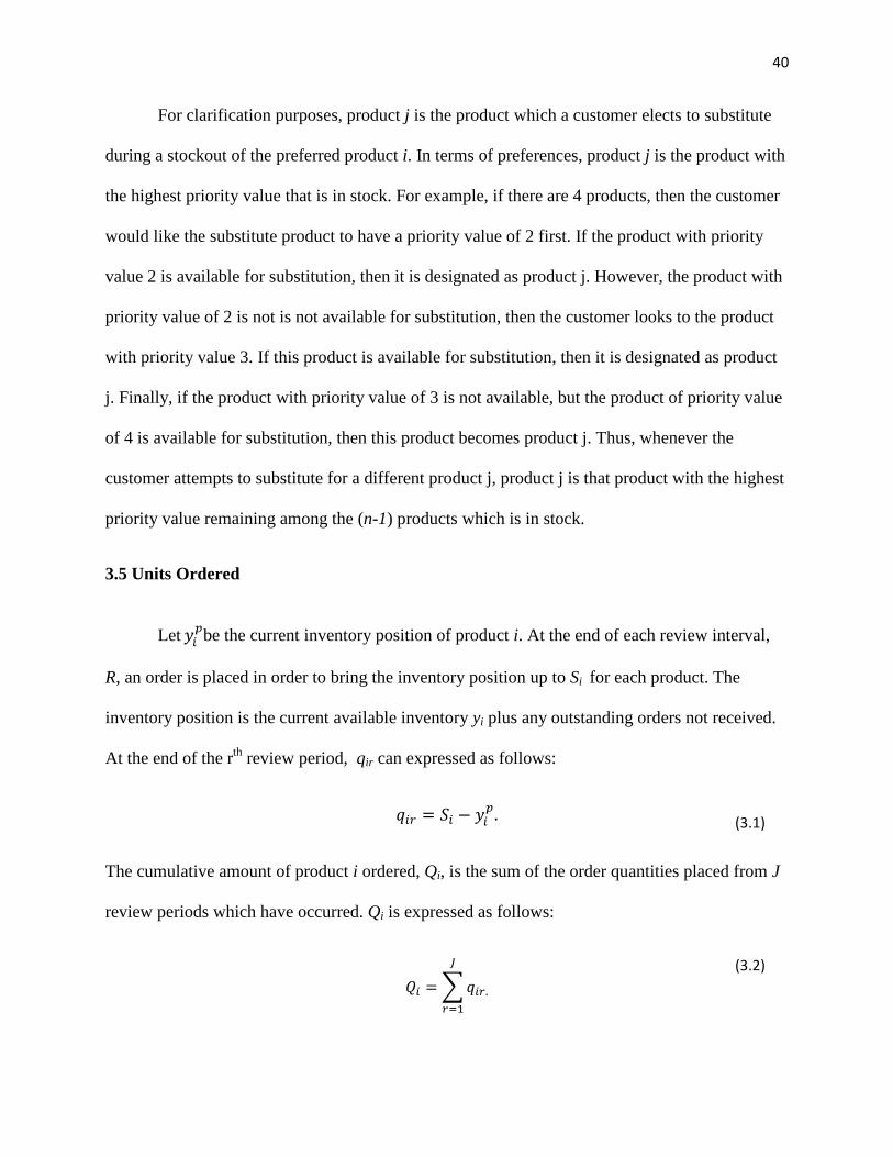
40

For clarification purposes, product j is the product which a customer elects to substitute

during a stockout of the preferred product i. In terms of preferences, product j is the product with

the highest priority value that is in stock. For example, if there are 4 products, then the customer

would like the substitute product to have a priority value of 2 first. If the product with priority

value 2 is available for substitution, then it is designated as product j. However, the product with

priority value of 2 is not is not available for substitution, then the customer looks to the product

with priority value 3. If this product is available for substitution, then it is designated as product

j. Finally, if the product with priority value of 3 is not available, but the product of priority value

of 4 is available for substitution, then this product becomes product j. Thus, whenever the

customer attempts to substitute for a different product j, product j is that product with the highest

priority value remaining among the (n-1) products which is in stock.

3.5 Units Ordered

Let be the current inventory position of product i. At the end of each review interval,

R, an order is placed in order to bring the inventory position up to Si for each product. The

inventory position is the current available inventory yi plus any outstanding orders not received.

At the end of the rth review period, qir can expressed as follows:

The cumulative amount of product i ordered, Qi, is the sum of the order quantities placed from J

review periods which have occurred. Qi is expressed as follows:

(3.1)

(3.2)

41

3.6 Updating Inventory Age

Let = (yi1,t, yi2,t, …, ) represent the vector of current inventory held at the each age

class during the tth day. The quantity to be delivered at the beginning of day t+l is qi(t-L). As a

transition is made from day t to t+1, can be expressed as follows:

Let wit represent the number of units of product i that expire at the end of day t. Thus, at the end

of day t, wit is

where is an element of the vector of . The cumulative expired product after D days can

be expressed a

3.7 Profit Function

Let πi represent the current cumulative profit for product i. πi which can be written as:

(3.3)

(3.4)

(3.5)

(3.6)

42

Thus, the overall total current profit for all n product variants, Π, is expressed as follows:

3.8 Optimization Problem

The retailer is faced with the problem of choosing Si for each product i in order to

maximize expected profit under demand uncertainty. The overall product class demand X, is a

random variable with p.d.f. f(x) and parameters, μ and σ. Each product variant i, accounts for a

proportion, κi, of the total demand for the product class. The order up to level for each product i,

Si, must be a non-negative integer quantity. The resulting mathematical programming problem is

expressed as:

Subject to:

Si is integer,

Si ≥0 ,

3.9 Newsvendor Model as a Special Case

The newsvendor problem is a special case of the perishable inventory problem. In the

newsvendor problem, Q is ordered once to meet demand over a single period knowing that all

items will expire after the end of the period. For the single product case, the vendor must select

(3.7)

(3.8)

(3.9)

(3.10)

43

Q* for a single product in order to minimize expected costs or maximize expected profit, where

at the end of the period, all unsold product expire. Q* is the smallest value of Q that satisfies the

following expression (Silver et al 1998):

where F-1 is the inverse of the cumulative distribution function of demand, cu is the marginal cost

of understocking the product, and co represents the marginal costs of overstocking the product.

The argument of F-1, i.e. the ratio of the costs on the right-hand side of (3.11) above is known as

the optimal cycle service level (CSL) or P1 which can also be referred to as the newsvendor ratio

(Nagarajan and Rajagopalan 2008).

In the problem scenario discussed in this thesis, there are multiple products involved and both

age-based and product based substitution. In a single period model, there is less of a distinction

between fresh and old products. Therefore, age-based substitution is much less of a factor or may

not be a factor at all. Product-based substitution, however, can still be relevant, as a consumer

could choose to substitute with a different product if the preferred product is not available.

A closed form solution can be developed considering n products. For the single period,

multi-item case, separate order quantities would be placed for each product i according to cost

parameters that comprise the cost of understocking, cui and overstocking coi for product i. It can

be shown that Qi satisfies the following (Silver et al 1998):

(3.12)

(3.11)

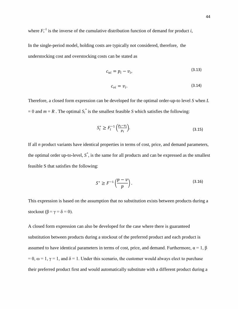
44

where Fi-1 is the inverse of the cumulative distribution function of demand for product i,

In the single-period model, holding costs are typically not considered, therefore, the

understocking cost and overstocking costs can be stated as

Therefore, a closed form expression can be developed for the optimal order-up-to level S when L

= 0 and m = R . The optimal Si* is the smallest feasible S which satisfies the following:

If all n product variants have identical properties in terms of cost, price, and demand parameters,

the optimal order up-to-level, S*, is the same for all products and can be expressed as the smallest

feasible S that satisfies the following:

This expression is based on the assumption that no substitution exists between products during a

stockout (β = γ = δ = 0).

A closed form expression can also be developed for the case where there is guaranteed

substitution between products during a stockout of the preferred product and each product is

assumed to have identical parameters in terms of cost, price, and demand. Furthermore, α = 1, β

= 0, ω = 1, γ = 1, and δ = 1. Under this scenario, the customer would always elect to purchase

their preferred product first and would automatically substitute with a different product during a

(3.13)

(3.14)

(3.15)

(3.16)

45

stockout of the preferred product. There is also the restriction that the order-up-to level must be

the same for all products. This case of full substitution among products during a stockout is also

known as risk pooling. First, the aggregate order-up-to level, , is determined by choosing

the order-up-to level S that satisfies (3.20). The optimal order-up-to level under risk pooling,

, is determined as follows:

If is non-integer, it is chosen from the surrounding integers that yield the higher

expected profit.

Understanding the relationship between S* and in the newsvendor model is useful

in gaining some insight into how the optimal Si values will change under varying operating

conditions for the general problem of an (R,Si) system with product perishability and

substitution. The relationship of S* to may depend on cost ratios, represented by the CSL

in the newsvendor problem. Let F(X) be the c.d.f. of demand X when there is no substitution and

G(X) be the c.d.f of demand X when there is full substitution. Based on the newsvendor model

and the assumption of identical parameters among products, the following three theorems apply:

Theorem 3.1: When F(X) > G(X), > S*

Theorem 3.2: When F(X) = G(X), = S*

Theorem 3.3: When F(X) < G(X) , < S*

(3.17)

46

Proofs of these theorems are outlined in Appendix A. The relationship of S* and Spooled* depend

on the relationship of F(X) to G(X). This shows that risk pooling does not always lead to a

reduction in the optimal S level, and consequently, inventory level, as is the case when F(X) ≥

G(X).

The simulation-optimization methodology will be necessary to determine the optimal S

values under departures from this special case of the newsvendor model. Nevertheless, it is

beneficial to have a closed form expression for the newsvendor case in order to validate the

results from the simulation-optimization for the special case of the (R,Si) system. Even though a

closed-form expression is developed for the special case, its evaluation may be difficult. In

addition, the closed form expression can be used to determine lower or upper bounds on S and

also can be helpful in developing tractable heuristics.

3.10 Simulation Model

Part of the proposed methodology in this thesis involves the construction of a simulation-

optimization model to find the best order-up-to level of inventory which maximizes expected

profit in an (R, Si) periodic review system. The first step of a simulation-optimization model is

the design of the simulation model.

Let l be the length of a simulation run and K be the number of replications of a simulation

run. The mean profit per simulation run of length l is estimated based on K replications and is

expressed as follows:

(3.18)

47

The standard deviation of the profit per simulation run, sl is expressed as

It is assumed that four major events occur over time, and the performance statistics will be

collected after a certain warm-up period once the performance characteristics reache a steady

state. The warm-up period will be determined based on Welch’s graphical procedure (Law and

Kelton 2000), which will be discussed in Chapter 4. Below is a list of the 4 major event routines

in the discrete-event simulation model.

1) Update Inventory Age Event – Going from period t to period t+1, is

determined according to (3.3) and outdated product, Wit, is updated by using to (3.4) and

(3.5).

2) Order Event – The order quantity in rth review period, qir, is determined by (3.1) and the

order arrives after the lead time elapses. The order-up-to Si level is set prior to the

simulation run.

3) Generate Demand Event-Daily customer demand is generated for each product based

on an adopted distribution f(x) with a mean and standard deviation of μ and σ. Each

arrival is then scheduled to occur randomly throughout the day and each customer

demands one unit of product. Demand is determined for each product variant based on κi

for all n product variants under consideration.

(3.19)

48

4) Sales Event –Based on inventory availability and the substitution dynamics, either a unit

is sold or its demand is lost. Zi and ζi are updated based on inventory availability and the

customer’s decision to substitute.

The following flow charts illustrate the logic within each event routine in the simulation model.

49

Figure 1: Event routines for inventory aging, ordering, and daily demand generation

2. Order Event

Set order quantity based on (3.1).

Update total units order based on (3.2)

Return

Schedule delivery after incurring lead

time

Schedule next order after R time

units

3. Generate Demand Event

Generate Demand for each product i

Schedule the arrival of each unit of

demand during the day.

Return

Schedule next Demand Generation

in 1 day

1. Update Inventory Age Event

Update inventory age vector based on (3.3) for all n products

Update expired product based on (3.5) for all n products

Schedule next inventory aging in 1 day

Return

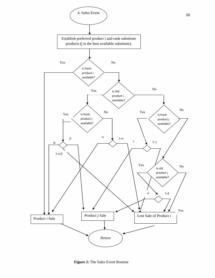
50

Figure 2: The Sales Event Routine

α

Product i Sale Lost Sale of Product i

Return

Product j Sale Yes

1-δ

1-α-β

Is old product j available?

Yes Is fresh product j available?

1-γ

No Is fresh product j available?

Is Old product i available?

Yes No

No

4. Sales Event

Establish preferred product i and rank substitute products (j is the best available substitute).

Yes

Is fresh product i available?

Yes

ω β

1-ω

γ

No

No

δ

Yes

51

The simulation model together is developed with the widely used software package

Arena. It is a general purpose simulation package that is highlighted in Law and Kelton (2000).

Modeling constructs, called “modules” are arranged into a number of categories and can be

easily dragged down to form a flow chart that represents the discrete events involved in the

modeled environment. Arena has limited (yet incredibly large) number of random-number

streams; for practical purposes it is virtually unlimited.

3.11 Simulation-Optimization Model

The simulation procedure is augmented through the addition of an optimization routine to

the discrete-event simulation model. Candidate solutions are generated by efficient search

techniques used in the optimization routine, and then the objective function values for the

candidate solutions are evaluated after K replications of the simulation model. Arena contains an

optimization package called OptQuest for Arena. The overall simulation-optimization model is

illustrated in Figure 3 below:

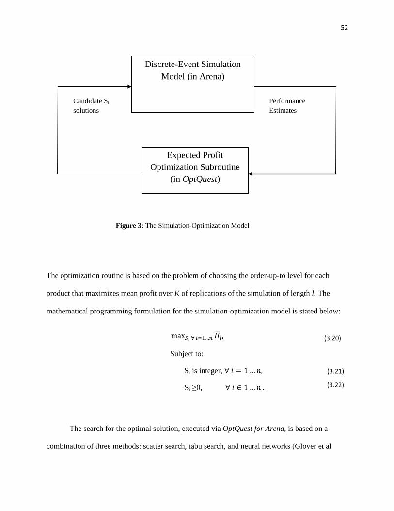
52

The optimization routine is based on the problem of choosing the order-up-to level for each

product that maximizes mean profit over K of replications of the simulation of length l. The

mathematical programming formulation for the simulation-optimization model is stated below:

Subject to:

Si is integer,

Si ≥0,

The search for the optimal solution, executed via OptQuest for Arena, is based on a

combination of three methods: scatter search, tabu search, and neural networks (Glover et al

Discrete-Event Simulation Model (in Arena)

Expected Profit Optimization Subroutine

(in OptQuest)

Candidate Si solutions

Performance Estimates

Figure 3: The Simulation-Optimization Model

(3.21)

(3.22)

(3.20)

53

1999). Scatter search operates on a set of solutions, called the reference set, and produces new

solutions based on a linear combination of existing solutions. The tabu search involves

improving the search procedure through recording the attributes of moves or solutions into a list

which rules out some undesirable moves for improved future moves. The neural network

component in the search routines also enhances the search by screening out solutions that are

likely to be poor without having to go through the full evaluation involved with the combined

scatter search and tabu search algorithms. Based on past information collected on the objective

function values and candidate solutions, the neural network routine attempts to develop decision

rules based on historical data that are continuously updated with each new solution. All together,

the three search techniques combine to result in an efficient search process that helps to find the

best solution based on the predefined objective.

While performing optimization through simulation, there may not be a guarantee of an

optimal solution. As the feasible solution space increases, the time to search within the feasible

region also increases. The establishment of legitimate upper and lower bounds on decision

variables can reduce the search time and also guarantee at least a local optimal solution once all

the candidate solutions have been evaluated. Whether or not the solution is globally optimal will

depend on the shape of the objective function. In order for a solution to be considered optimal in

the sense of stochastic optimization, it must produce an objective value that cannot be improved

by any other candidate solutions in a statistically significant fashion. replications performed for

each candidate solution represents a random sample from the population of all potential

replications that represent unique realizations of any random variables built in the simulation

model. The number of replications generally used to compare candidate solutions will be

relatively large, so the concepts of the central limit theorem can be applied when comparing the

54

objective function values among multiple solutions. Therefore, for each simulation-optimization

trial, the Si values that produce the best average profit value will be identified with the use of

reasonable lower and upper bounds that will be further discussed in Chapter 4.

3.12 Summary

This chapter has provided the foundation of how to model an (R,Si) system under product

perishability and substitution. A methodology has been proposed that in order to determine the Si

values that attempts to maximize expected total profit. It is important that the system of

managing multiple substitutable, perishable products is accurately modeled and the

subcomponents of the simulation-optimization model such as product demand and substitution,

inventory aging, and the profit function must be carefully designed in order to give validity to the

numerical results. Closed form expressions have been developed for special cases of an (R,Si)

system with product perishability and substitution that can be used to validate the results from

the simulation-optimization, develop lower and upper bounds on the optimal Si values for other

cases, and also develop simple heuristics, applicable from the standpoint of practitioners.

55

Chapter 4: Experimental Design for Simulation-Optimization Study

4.1 Overview

This chapter outlines the experimental design for the simulation-optimization study

involving an (R,Si) system for substitutable and perishable items. The selection of parameters

values is addressed for the range of operating conditions and the simulation-optimization runs.

Eventually, the goal is to be able to use the results to understand the impact of changes in input

parameters such as substitution, shelf-life, cost structures, lead time, and number of products on

the optimal Si values and the corresponding expected total profit while keeping other parameters

constant.

The organization of this chapter is as follows. Section 4.2 concerns additional

assumptions for the simulation-optimization study, Section 4.3 deals with the fixed and varied

input parameters in the factorial design, and in Section 4.4, the performance measures and other

outputs are discussed. Section 4.5 covers the characteristics of the simulation model while

Section 4.6 addresses the specific settings dictated for the corresponding optimization routine.

Finally, Section 4.7 is a summary of the chapter.

4.2 Additional Assumptions

56

There are additional assumptions that will be made for the purposes of the simulation-

optimization study. These assumptions concern the shelf life of a product, arrival time of each

unit of demand within a particular day, and the distribution of demand.

It is assumed that the shelf life of a product must be at least the length of a coverage

period which includes the review period, R, and lead time, L. This implies the following

relationship:

If the shelf life of a product were less than the cycle length, then there would be a guarantee that

all inventory items would expire within a given cycle and an increased risk of a stockout during a

review cycle.

The demand for a product is a discrete random variable. In Chapter 3, it was pointed out

that either a discrete probability distribution could be used or a continuous distribution where the

realization of demand is rounded to the nearest integer. For the purposes of the initial simulation-

optimization study, it is preferable to use a discrete distribution in order to have a better

understanding of the results and enhance the development of a heuristic. The heuristic can then

be tested using multiple demand distributions, either discrete or continuous.

Overall demand for a product class will be assumed to follow a negative binomial

distribution. The advantages of the negative binomial for discrete product demand is discussed

in (Law and Kelton 2000) and (Ferguson and Ketzenberg 2006). For the factorial design, the

mean, μ, and standard deviation, σ, of product demand will be fixed. Let CV represent the

coefficient of variation of product demand. Therefore, CV is the ratio of the standard deviation to

57

the mean of product demand. The CV of demand will remain constant in the simulation-

optimization study, but for the testing of a proposed heuristic, the CV will be allowed to vary.

Finally, although the price and unit cost can vary for each product variant within a

product class, the profit margin, defined as retail price minus unit purchase cost, is assumed to be

the same for each product. This assumption is adopted in order to eliminate a retailer’s incentive

to overstock a product that would be more profitable. If the profit margin of two items are

consideration are the same, but the unit purchase cost and retail price differ, some interesting

dynamics may be observed under product-based substitution. More revenue is generated by sales

of an item with a higher retail price, but an item with a higher unit purchase cost is in essence

more costly to dispose. It is of interest to analyze how retail price and unit purchase cost can

affect optimal inventory policy under product-based substitution.

4.3 Fixed and Varied Parameters for the Simulation-Optimization Study

For the purposes of an experimental design for the simulation-optimization study, it is

important to determine which parameters are to be fixed and which are to vary. The demand

distribution, mean demand, coefficient of variation of demand, and variation of market share of

each product will be held constant while the length of review period, lead time, number of

products, shelf-life of products, coefficient of variation of demand, proportion of overall demand

for each product, price, holding cost, and substitution factors will all vary. This factorial design

will be applied to the case of two and three product variants within a product class. However, in

the case of three product variants, it will be assumed that all products have similar properties in

terms of demand and cost structures. Therefore, Si will also be assumed to be the same for all

products. It is of interest to analyze the impact of an additional product variant keeping overall

58

product class demand constant. Finally, one major objective of this study is to develop a heuristic

for the n=2 product case that can work well under varying operating conditions. Table 1 below

summarizes both the fixed and varied input parameters for the simulation-optimization study

Fixed Input parameters Level Demand distribution Negative Binomial

μd 22

CV 0.7 Factors Levels

N 2,3 items R 2,3 days L 0,1 days

mi 4,6 days

E(κi) Equal, Unbalanced

hi $0.0083/unit/day, $0.0833/unit/day

pi $4,$5 vi $1,$2

Product Based Substitution High, Low Age Based Substitution High, Low

Table 1: Fixed and varied parameters for simulation-optimization study

59

Overall, a total of 696 distinct combinations of the parameter values in Table 1 above will

be evaluated out of a possible 210 = 1024. This is a fractional factorial design as some parameter

combinations will be eliminated due to redundancy and necessity based on the intentions of this

study. Since the n = 3 case for number of products introduces more complexity and takes longer

to search for the optimal solution, only the special cases are evaluated where all products are

assumed to have identical properties in market share, costs, and shelf-life. In this case, it can be

easily assumed that the order-up-to level will be the same for all three products. Based on the

parameters chosen, there are 96 combinations of parameters that will be evaluated for the n = 3

case and 600 combinations of parameters for the n = 2 case. Of the 600 for the n = 2 case, 96 of

the combinations will be identical to the 96 chosen for the n = 3 case, and the remaining 504

combinations will involve two products that have at least one property that differs from the other.

The ultimate goal of this study is to be able to examine the effects of factors such as product-

based substitution, age-based substitution, lead time, shelf-life of products, cost structures, and

number of products on the simulated optimal solutions.

The fixed parameters concern properties of product demand. The overall daily market

demand will follows a negative binomial distribution with a mean of 22 and standard deviation

of 0.7. The expected market share for each product will vary between 0.5 and 0.7; however, there

is uncertainty in this parameter. A uniform distribution will be assumed for the market share of a

product. In other words, the realized market share of a product can fall anywhere within 0.2 of

the expectation in this two product case. For example, if the expected market share is 0.7 for a

particular variant, then the realized market share can be anywhere from 0.5 to 0.9. This equates

to a standard deviation of 0.033. This standard deviation of market share will remain constant

throughout the study.

60

As for the varied parameters, the review period will be either 2 or 3 days and lead time

will be zero or 1 day. However, only the following review period/lead time pairs are to be

evaluated: (2,0), (2,1), and (3,0). Having (2,1) vs. (3,0) enables a comparative study on the effect

of lead time on optimal stocking levels. Having (2,0) offers a smaller cycle length and allows for

the examination of how optimal inventory policy is affected by increased shelf-life relative to the

coverage period. Thus, it is decided that (3,1) is not necessary for inclusion in the simulation

study as it will only yield marginal additional information.

The shelf-life of the products will vary between 4 and 6 days. It is possible for two

product variants to have different shelf-lives. In all scenarios examined, the shelf-life of each

product will exceed the cycle length. The maximum differential between product shelf-life and

cycle length, therefore, is 4 days.

In terms of cost structure, there will be two scenarios for the marginal holding cost, hi,

applied to average inventory based on the length of the simulation run. One scenario is that the

holding cost is relatively low, $0.0083 per item per day and the other scenario is that the

marginal holding cost is relatively high, $0.0833 per item per day. These values are arbitrarily

chosen and represent a stark contrast between what can be perceived as low versus high holding

cost. The retail price will vary between $4 and $5 while the unit purchase cost will vary between

$1 and $2. One requirement for the price and unit purchase cost is that the margin, pi-vi, must be

the same for each product. Thus, the profit margin for each product will be either $2, $3, or $4.

In terms of substitution, there are two levels for both product-based and age-based

substitution. A high level of product-based substitution with high level of age-based substitution

will translate to (α = 0.4 β = 0.5, ω = 0.8, γ = 0.8, and δ = 0.7), high level of product-based

61

substitution with low age-based substitution will translate to (α = 0.2 β = 0.7, ω = 0.3, γ = 0.8,

and δ = 0.2), low level of product-based substitution with high age-based substitution will

translate to (α = 0.7, β = 0.2, ω = 0.8, γ = 0.3, and δ = 0.2), and a low level of product-based

substitution with low age based substitution will translate to (α = 0.2, β = 0.2, ω = 0.3, γ = 0.3,

and δ = 0.2).

4.4 Performance Measures and Other Selected Outputs

For a particular simulation run, it is necessary to also decide on which performance

measures and output variable values to collect. Since the problem is to find the Si values that

maximize expected profits, then total profit is one performance measure that needs to be

observed every simulation run. In addition, based on the best Si values, the CSL or P1 service

level measure can be derived. Other performance measures to be recorded are total sales of

product (Zi), total lost sales of product i (ζi), and total expired unit of product i (Wi). For the

purpose of warmup determination, the average inventory level, will also be recorded. The

sample mean based on K replications will be used to estimate the true expectation for each of the

performance measures.

In addition to the performance measures listed above, one additional output to be tracked

is total demand of product i. Based on replications, a mean value will be obtained for the total

demand of product i. It is of interest to collect this output measure to ensure that the random

number seed is producing consistent values that will produce consistent product demand

realizations for each replication.

4.5 Simulation Parameters

62

After establishing the parameter values for the factorial design, it is also necessary to

define characteristics regarding the simulation run and the corresponding optimization process.

Time is expressed in hours and it will be assumed that one working day is equal to 15 hours

which are typical of grocery stores. Since a review period is expressed in days, the choice of

operating hours in one day should not impact the model. It is also assumed that there are 7

working days in a week and no holidays are incorporated into the model.

Two key simulation parameters that must be carefully selected are the warm-up period

and simulation run length, w and l. A warm-up period is necessary to deal with the initialization

bias with regard to the simulation variable. Welch’s graphical procedure can be used to

determine appropriate value of w (Law and Kelton 2000). The choice of output measure used for

the procedure was the average inventory for one variant for the n = 2 case. The average inventory

value was recorded every 15 hours for up to 1500 hours of simulation run length and the

procedure is repeated for 10. The selected values of the relevant input parameters that impact

average inventory for a given simulation run are S1 = 30, S2 = 30 , μ = 20, cv = 0.9, equal

expected proportions of overall demand for each product, R = 3, and L = 1. All other system

variables for this procedure are set to zero at the beginning of the run. The graph below

represents a plot of the mean average inventory at each time interval based on 10 replications.

63

Based on the graph, a warm-up period of 450 hours was selected. This seems to be a reasonable

point where the average inventory appears to reach steady state. Therefore, data for the first 450

hours will be discarded.

The next issue regarding the simulation run is the choice of l. Depending on the problem,

precise methods like Welch’s procedure could be used to also determine l. In this case, the

choice of l is at 1350 hours. Based on the graph, it appears that the average inventory is fairly

20

25

30

35

40

45

50

0 100 200 300 400 500 600 700 800 900 1000 1100 1200 1300 1400 1500

Prod

uct 1

Ave

rage

Inve

ntor

y

Time(Hours)

Product 1 Mean Average Inventory Over Time (10 Replications)

End of Warm-up Period

End of Simulation Run

Figure 4: Welch's Graphical Procedure for determining warm-up period and replication length

64

stable at this point. The net simulation run length in consideration of the warmup period becomes

900 hours. This equates to 60 operating days, which would be approximately two months.

4.6 Simulation-Optimization parameters

For the simulation-optimization model, there is also some parameter selection that needs

to be addressed. One issue is in the choice of K, the number of replications to be used for each

simulation. One feature of OptQuest is that you can set the desired level of precision in

estimating the mean. In this case, it will be desirable to estimate the mean with a sampling error

of 2%. Therefore, for every candidate solution, the number of replications is the minimum

number needed to estimate the mean within 2% sampling error. This can vary based on the

operating conditions selected.

Another important set of parameters regarding the simulation-optimization model are

lower and upper bounds on the Si values. Based on the assumptions for the problem, each Si

value must be a non-negative integer value. It is advantageous to impose lower and upper

bounds, SL and SU, respectively, in order to speed up the search and narrow the feasible region.

Since a closed form solution exists for the newsvendor model, this can be used to help set the

lower and upper bound for the search of the best S value in the problem of managing identical

substitutable and perishable items. Given a coverage period of (R+L), let Snv represent the

optimal S value based on (3.16) if the scenario was a newsvendor model where m = (R+L) and

there is no substitution between products. Snv is believed to be closer to a lower bound than an

upper bound since it is expected that the optimal S level will increase as m increases. Thus, the

lower and upper bound, SL and SU will be set as follows:

65

The choice of the coefficients 0.75, and 1.5 are arbitrary. If SL is non-integer, then it will be

rounded down to the nearest integer, and if SU is non-integer, then it will be rounded up to the

nearest integer. If the optimal solution ends up being either SL or SU, then more candidate values

either below SL or above SU will be evaluated in an attempt to determine the true globally optimal

Si values.

4.7 Summary

The experimental design for the simulation-optimization analysis has been carefully

planned out in order to gain the necessary insight into the factors that impact the optimal Si levels

for identical substitutable and perishable goods. In addition, careful measures have been taken to

also ensure the validity of the procedure. In order to efficiently execute the experiment, lower

and upper bounds have been placed on the candidate Si values for each simulation run. If the best

Si value falls on or near any of the two bounds, then the bounds can be relaxed to ensure that the

true optimal solution is not missed. Chapter 5 provides the results and analysis from the factorial

design simulation-optimization study.

66

Chapter 5: Simulation-Optimization Study Results and Analysis

5.1 Overview

This chapter reports on the results from the simulation-optimization study and

analyses the effects of the factors of substitution, shelf-life, lead time, and cost structures

on the simulated optimal order-up to levels of inventory. As described earlier, a total of

696 scenarios are evaluated using a simulation-optimization model through OptQuest for

Arena. In every case, and exhaustive search of the feasible region is executed to produce

the simulated-optimal solution. Statistical tests are performed on the results to conclude

on the significance of any effects attributed by these factors. As discussed in the previous

chapter, 600 of the scenarios involve two products while 96 of the scenarios include three

products. The detailed results from the n = 2 case are included in Appendix B while the

results from the n = 3 case are found in Appendix C. The case of three products assumes

that all three products have identical properties. Thus, for simplicity, it is also assumed

that each product will have the same order-up-to level under these settings. However, for

the case of dissimilar products, there can be at least one property that distinguishes one

product from another. In this case, the order-up-to levels are allowed to differ.

The organization of this chapter is as follows. Section 5.2 deals with the concepts

of service level and allocation while Sections 5.3-5.8 provide analysis of the effect of

substitution, cost properties, shelf-life, lead time, and number of products respectively.

67

Finally, Section 5.8 gives a summary of the results and analysis from the simulation

optimization study.

5.2 Service Level and Allocation

There are two important components in the optimal order-up-to levels of the two

products. One component is the aggregate order-up-to level of all products and the other

component is the allocation of the aggregate order-up-to level to each product. It is

believed that both the aggregate order-up-to level and the allocation will vary according

to changes in the factors considered in the study.

The results from the simulation study will be used for the development of a

heuristic technique for the inventory policy involving products under product substitution

and perishability. Since only a limited span of parameter values is used for the

simulation-optimization study, it is important that the heuristic developed can be

applicable over a wider range of values. One method that can help to ensure this is to

standardize the measure of the aggregate order-up-to level for all products. The aggregate

order-up-to level value can be transformed into an aggregate service level measure based

on the properties of the product demands. This is a theoretical notion of service level but

not the actual observed service level. Since product substitution and perishability is

factored into the problem, the observed service level may not equal the theoretical

notion.This is similar to the concept of the CSL in the newsvendor model. The right-hand

side of the equation, which is the ratio of understocking costs to total costs, represents the

optimal cycle service level. The service level discussed in the remainder of this thesis

will pertain to the CSL equated with the aggregate order-up-to level. Since the demand

68

parameters are known in the simulation study, the aggregate order-up-to level can be

easily transformed to the service level measure for each scenario as is done in the case of

the newsvendor model explained in Chapter 3.

For example, assume that overall product demand for apples is normally

distributed with a mean of 40 units per day and a standard deviation of 20 and that there

are two product variants: red delicious apples with 30% as the expected market share and

golden delicious apples with an expected market share of 70%. Assume that based on all

other operating conditions under consideration, the optimal order-up-to level for red

delicious is determined to be 25 while the optimal order-up-to level for golden delicious

is determined to be 30. If this is the case, we can also say that the aggregate order-up-to

level for apples is 55 and the optimal allocation is 25/55 or 45.45% (15.45% greater than

expected market share) to golden delicious apples and 30/55 or 54.54% (15.45% less than

expected market share) to red delicious apples. In order to convert the aggregate order-

up-to level into the CSL measure, we can determine the probability that market demand

for apples is less than or equal to 55. Based on the fact that demand is normally

distributed, the CSL would be equal to 0.7733. The observed service level for an

aggregate order-up-to level of 55 may be different than 0.7733Therefore, the CSL service

level measure and allocation measures will be used as a way to normalize the response

variable under changes in operating conditions.

The negative binomial distribution is used to model product demand in the

simulation-optimization study. Daily demand is assumed to be stationary in that the mean

and variance of daily demand remain constant throughout the length of a simulation run.

One convenient property of the negative binomial distribution is that the sum of

69

independent negative binomial random variables with identical properties also follows a

negative binomial distribution (Singh et al 2007). In order to determine the parameters of

demand during the review period plus lead time, this property can be applied based on the

fact that each day is independent of the other. The aggregate order-up-to level can be

used to compute this aggregate service level by determined the probability that total

demand is less than or equal to the aggregate order-up-to level based on the negative

binomial distribution with parameters adjusted for the length of the coverage period

(R+L).

5.3 The effect of substitution on service level

One major objective of this study is to examine the effect of substitution on

inventory policy. There are two types of customer substitution identified as possibilities

in consumer behavior, namely product-based substitution and age-based substitution.

With product based substitution, the customer elects to purchase a substitute product

variant when the preferred variant is out of stock. The other type of substitution is age-

based where it is assumed that a customer prefers to purchase fresh product first, and may

substitute an older state of the same product if the fresh is out-of-stock. As mentioned

earlier, fresh items are defined as those that have at least half of their shelf-life remaining

while old items are defined as those that have less than half of their shelf-life remaining.

The levels of substitution examined in the simulation optimization study are

classified based on the ordered pair that denotes both the product-based substitution level

and age-based substitution level. For each type, there is either a high or low level, and the

specific parameter values given for each substitution parameter are explained in the

70

previous chapter. It is of interest to assess how the levels of substitution affect both the

aggregate service level based on the aggregate order-up-to level of the two products and

the percentage of the aggregate order-up-to level allocated to each product.

Theorems 3.1, 3.2, and 3.3 suggest that cost structures can interact with

substitution under the risk pooling concept with the newsvendor model. The cycle service

level in the newsvendor model is based on the ratio of the costs of understocking to the

sum of over and understocking costs. For this study, there are three cost combinations.

The effect of risk pooling can potentially vary according to how the cycle service level

changes. Thus, the tests of the substitution effect will be organized according to cost

properties of the two product variants.

Overall, the 600 scenarios for two products can be subdivided into the following

three categories according to adopted cost structures:

• Category 1 includes all scenarios where the unit selling price of each product is

$4 while the unit purchase cost is $2.

• Category 2 includes all scenarios where one product has a unit selling price of $4

and a unit purchase cost of $1, while the other product has a unit selling price of

$5 and a unit purchase cost of $2.

• Category 3 includes all scenarios where the unit selling price is $5 and the unit

purchase cost is $1.

Table 2 below is a summary of the average service level according to the level of

substitution and cost category for the 600 scenarios evaluated. For the substitution levels

illustrated in the table, HH represents a high level of product-based substitution paired

with a high level of age-based substitution, HL represents a high level of product-based

71

substitution paired with a low level of age-based substitution, LH represents a low level

of product-based substitution paired with a high level of age-based substitution, and LL

represents a low level of product based substitution paired with a low level of age-based

substitution.

72

Substitution

Cost Category

1 2 3

Avg. service

level Avg.

Profit

Avg. service

level Avg.

Profit

Avg. service

level Avg.

Profit HH 0.7261 2043.756 0.8559 3347.632 0.9027 4677.874 HL 0.6418 1829.236 0.8129 3031.52 0.8865 4296.987 LH 0.7173 1996.012 0.839 3282.986 0.9101 4615.017 LL 0.612 1762.562 0.777 2908.935 0.8797 4139.92

The effect of substitution on service level for cost each category is evaluated

through one-way ANOVA. All relevant statistical output for the ANOVA tests is

included in Appendices D.1-D.6. There are some issues that need to be taken into

consideration with the one-way ANOVA procedure applied to this data. The assumptions

for ANOVA testing are that there is randomness and independence, normality, and

homogeneity of variance among the groups tested (Levine et al 2008). The randomness

and independence assumption is intact; however, there are potential issues with normality

and homogeneity of variance. Figures 5, 6, and 7 below illustrate the data collected for

the service levels for each type of substitution within the three cost categories.

Table 2: Average aggregate service level and profit based on substitution and cost category from the simulation-optimization study

73

0

0.1

0.2

0.3

0.4

0.5

0.6

0.7

0.8

0.9

Serv

ice

Leve

l

Substitution Characteristics (Product-Based,Age-Based)

Service Level vs. Substitution for Cost Category 1

High,High High,Low Low,High Low,Low

Figure 5: Service Level vs. Substitution for Cost Category 1

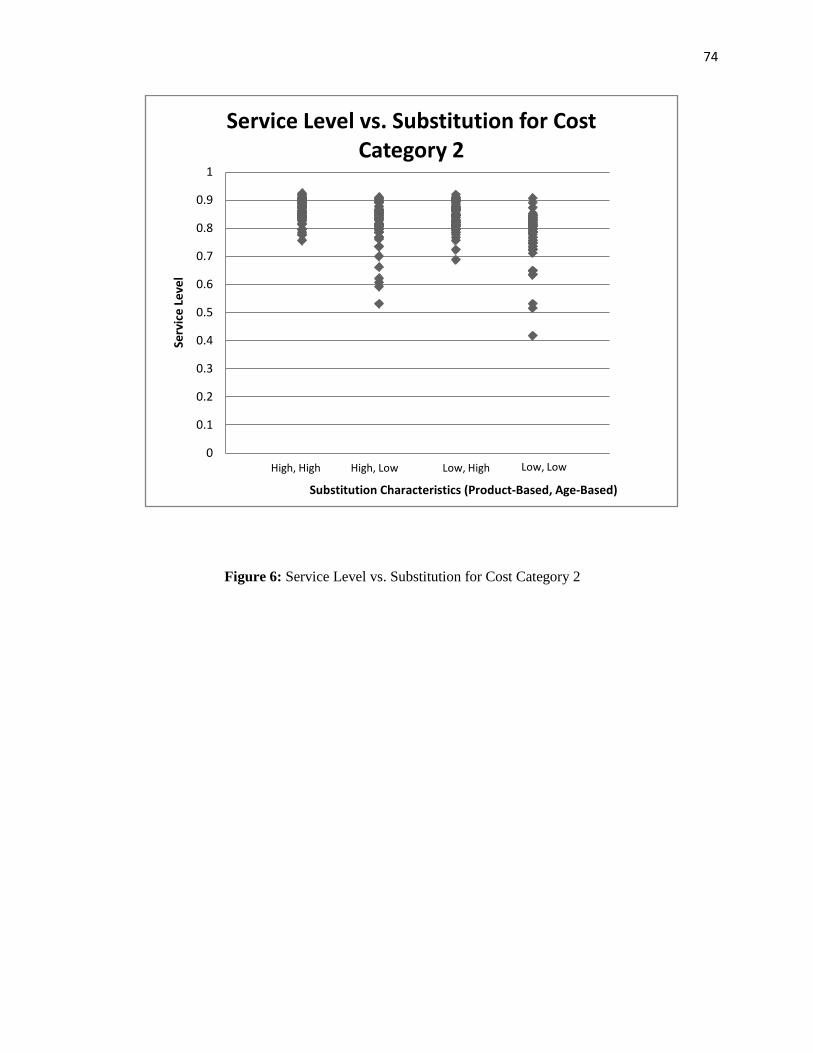
74

0

0.1

0.2

0.3

0.4

0.5

0.6

0.7

0.8

0.9

1Se

rvic

e Le

vel

Substitution Characteristics (Product-Based, Age-Based)

Service Level vs. Substitution for Cost Category 2

High, High High, Low Low, High Low, Low

Figure 6: Service Level vs. Substitution for Cost Category 2

75

Figures 5, 6 and 7, indicate that there appear to be differences in the distributions of

service levels both among the substitution levels within each type of cost category, and

across each cost category, suggesting that there is an overall interaction effect between

the nature of substitution and cost properties. Regarding the ANOVA tests, there could

potentially be issues with the normality and equal variance assumptions. Since the sample

sizes are fairly large (42 scenarios for each substitution level in cost categories 1 and 3

and 62 scenarios for each substitution level in cost category 2) and the fact that the

sample sizes are equal for each group within the category, the ANOVA tests are robust to

handle departures in normality and equal variances (Wackerly et al. 2002). Therefore,

proceeding with the ANOVA tests with this data is done with caution.

0

0.1

0.2

0.3

0.4

0.5

0.6

0.7

0.8

0.9

1

Serv

ice

Leve

l

Subsitution Characteristics (Product-Based,Age-Based)

Service Level vs. Substitution for Cost Category 3

High,High High,Low Low, High Low, Low

Figure 7: Service Level vs. Substitution for Cost Category 3

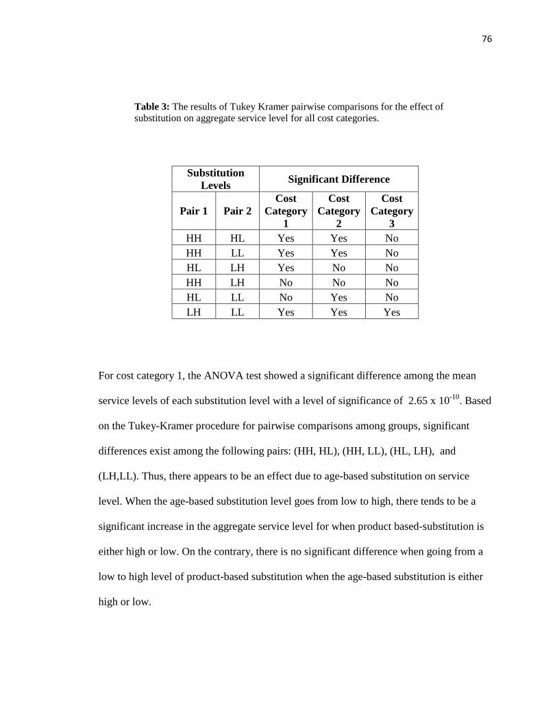
76

Substitution Levels Significant Difference

Pair 1 Pair 2 Cost

Category 1

Cost Category

2

Cost Category

3 HH HL Yes Yes No HH LL Yes Yes No HL LH Yes No No HH LH No No No HL LL No Yes No LH LL Yes Yes Yes

For cost category 1, the ANOVA test showed a significant difference among the mean

service levels of each substitution level with a level of significance of 2.65 x 10-10. Based

on the Tukey-Kramer procedure for pairwise comparisons among groups, significant

differences exist among the following pairs: (HH, HL), (HH, LL), (HL, LH), and

(LH,LL). Thus, there appears to be an effect due to age-based substitution on service

level. When the age-based substitution level goes from low to high, there tends to be a

significant increase in the aggregate service level for when product based-substitution is

either high or low. On the contrary, there is no significant difference when going from a

low to high level of product-based substitution when the age-based substitution is either

high or low.

Table 3: The results of Tukey Kramer pairwise comparisons for the effect of substitution on aggregate service level for all cost categories.

77

As in cost category 1, the ANOVA tests reveal a significant difference among the

aggregate service levels for each type of substitution for cost category 2. The statistical

significance is supported by a level of significance of 3.48 x 10-11. Based on the Tukey

Kramer procedure, significant differences exist among the following pairs: (HH, HL),

(HH, LL), (HL, LL), (LH, LL). Similar to cost category 1, there are four pairs with

differences; however, with cost category 2, there is a difference between HL and LL, but

not with HL and LH. For cost category 2 when age-based substitution is low, the mean

service level increases when going from low product-based substitution to high-product

based substitution. Thus, there is a conditional effect of both product-based and age-

based substitution on the aggregate service level under cost category 2.

As in the other two categories, analysis of cost category 3 also reveals a

significant difference among the mean service levels for each type of substitution based

on the level of significance of 0.005. However, based on the Tukey-Kramer procedure for

pairwise comparisons, there was only a significant difference in the (LH, LL) pair. When

the level of substitution goes from low to high for age-based substitution for the case of

low product based substitution, the mean service level increases. There is only a

conditional age-based substitution effect in this cost category since no difference is

concluded when going from low age-based substitution to high age-based substitution for

the case of high product-based substitution.

For all three cost categories, it is apparent that expected profit increases as the

level of substitution increases in both the product-based and age-based cases. Increased

substitutability allows for more opportunity for sales since the customer is more willing

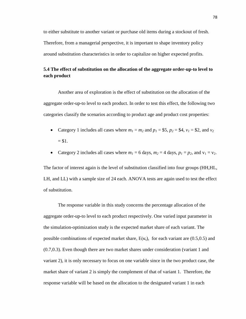
78

to either substitute to another variant or purchase old items during a stockout of fresh.

Therefore, from a managerial perspective, it is important to shape inventory policy

around substitution characteristics in order to capitalize on higher expected profits.

5.4 The effect of substitution on the allocation of the aggregate order-up-to level to each product

Another area of exploration is the effect of substitution on the allocation of the

aggregate order-up-to level to each product. In order to test this effect, the following two

categories classify the scenarios according to product age and product cost properties:

• Category 1 includes all cases where m1 = m2 and p1 = $5, p2 = $4, v1 = $2, and v2

= $1.

• Category 2 includes all cases where m1 = 6 days, m2 = 4 days, p1 = p2, and v1 = v2.

The factor of interest again is the level of substitution classified into four groups (HH,HL,

LH, and LL) with a sample size of 24 each. ANOVA tests are again used to test the effect

of substitution.

The response variable in this study concerns the percentage allocation of the

aggregate order-up-to level to each product respectively. One varied input parameter in

the simulation-optimization study is the expected market share of each variant. The

possible combinations of expected market share, E(κi), for each variant are (0.5,0.5) and

(0.7,0.3). Even though there are two market shares under consideration (variant 1 and

variant 2), it is only necessary to focus on one variable since in the two product case, the

market share of variant 2 is simply the complement of that of variant 1. Therefore, the

response variable will be based on the allocation to the designated variant 1 in each

79

scenario. The expected market share of variant 1 varies between 0.5 and 0.7. The

response variable in terms of allocation will be measured as the difference between the

simulated-optimal allocation to variant 1 and the expected market share. For example, the

S1* = 40 and S2

* = 10, and E(k) = 0.7, then the response variable would be the difference

between 0.8 (proportional allocation of the aggregate order-up-to level to variant 1) and

0.7 (expected market share of variant 1) which equals 0.1. Tables 4 and 5 below displays

the average differences in the percentage allocation of the aggregate order-up-to level to

variant 1 and the expected market share of variant 1 for each substitution level between

category 1 and category 2 and the results of the Tukey-Kramer Procedure for pairwise

comparison among the substitution levels in each category.

Substitution

Category 1 2

Avg. Allocation

diff. Avg.

Profit

Avg. Allocation

diff. Avg.

Profit HH -0.197 $3,297.68 0.1275 $3,426.55 HL -0.182 $2,968.25 0.0794 $3,164.69 LH -0.0615 $3,254.22 0.0432 $3,357.03 LL -0.0812 $2,874.71 0.0547 $3,007.14

Table 4: The results of the effect of substitution on the allocation of relative aggregate order-up-to level to each product, measured as the difference between

actual allocation and expected market share of product demand, and profits

80

For cost category 1, the ANOVA test reveals a significant difference among the mean

allocations to product 1 among the 4 types of substitution. The level of significance from

the test is 1.69 x 10-24 showing very strong evidence of such difference. The results from

Table 5 suggest that when going from low to high product-based substitution, the

allocation to product 1 changes for category 1. Under this category, the selling price of

product 1 exceeds that of product 2, but the unit purchase cost of product 1 is higher than

that of product 2. There is evidence that when the alternative of product-based

substitution is highly favorable among customers, it is advantageous for managers to

stock less of product 1 than its expected market share and more of product 2 than its

Substitution Levels Significant Difference

Pair 1 Pair 2 Category 1 Category 2 HH LH Yes Yes HH LL Yes Yes HL LH Yes No HL LL Yes No HH HL No Yes LH LL No No

Table 5: The results of the Tukey-Kramer Procedure for pairwise comparisons between substitution levels based on the allocation of aggregate order-up-to level to

each product

81

expected market share. Items with a higher unit cost correspond to a higher cost of

perishability. Under high product-based substitution, a shortage of inventory of one

product can be met by excess inventory of another product. The underlying assumption in

this study is that the profit margins are the same although the unit purchase cost and

selling price may be different. With a high level of substitution, if there is going to be

excess inventory, it is less costly for the excess to be in the product with the lower unit

cost. Hence, this is why the allocation to product 1 decreases when its unit cost is higher

than product 2 and the level of substitution is high.

Category 2 in this study involves all scenarios where the shelf-life of product 1

exceeds that of product 2, yet the both the unit selling price and unit purchase cost of both

products are identical. As in category 1, the one-way ANOVA test reveals a significant

difference among the four groups according to substitution with a level of significance of

1.19 x 10-05. The results from Table 5 indicate that with the category 2 case, the effect of

product-based substitution only turns out to be significant when the age-based

substitution is high. Contrary to the category 1 case, the effect of age-based substitution is

significant when product based-substitution is high. Thus, it is attractive to stock more of

product 1 than its market share when the shelf-life exceeds that of product 2 when going

from low to high product based substitution when age-based substitution is high. In

addition, it is desirable to stock more of product 1 than its market share when the shelf-

life exceeds that of product 2 when going from low to high age-based substitution and the

level of product-based substitution is high. A product with a greater shelf-life can be

stored in greater quantity since each item has an increased probability of being sold and

82

decreased probability of being lost to expiration. However, when age-based substitution

is low, there is a greater decline in the utility of consuming an older item, and the excess

quantity of old product has a greater chance of expiring. Under this scenario, the

advantage of stocking more of the longer lasting product tends to be neutralized.

Overall, there appears to be evidence of a substitution effect when dealing with

optimal inventory policy. Age-based substitution seems to play a more predominant role

in impacting aggregate service level while product-based substitution plays a larger role

in determining the allocation of the overall order-up-to level for each product. By the

differences that exist among the categories evaluated in both the service level ANOVA

tests and percentage allocation tests, the substitution factor at times can interact with cost

properties and the shelf-life factor.

5.5 The effect of cost structures on service level

Based on the analysis on the effect of substitution, there seems to be an indication

that the cost structures of the two products play a role in determining optimal inventory

policy. Earlier analysis on the newsvendor model demonstrated how the cycle service

level is based on the ratio of the costs of understocking to the sum of the costs of

understocking and overstocking. In the general perishable inventory problem for an (R,Si)

system, it is unclear whether or not the same or similar properties will hold when the

shelf-life of products exceed the cycle length. Therefore, it is of interest to statistically

evaluate the effect of cost properties on the overall service level achieved from the

aggregate order-up-to level of the two products.

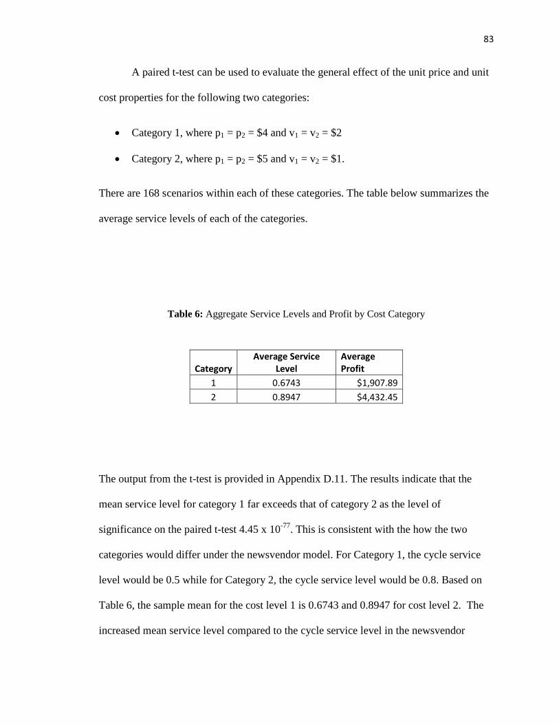
83

A paired t-test can be used to evaluate the general effect of the unit price and unit

cost properties for the following two categories:

• Category 1, where p1 = p2 = $4 and v1 = v2 = $2

• Category 2, where p1 = p2 = $5 and v1 = v2 = $1.

There are 168 scenarios within each of these categories. The table below summarizes the

average service levels of each of the categories.

Category Average Service

Level Average Profit

1 0.6743 $1,907.89 2 0.8947 $4,432.45

The output from the t-test is provided in Appendix D.11. The results indicate that the

mean service level for category 1 far exceeds that of category 2 as the level of

significance on the paired t-test 4.45 x 10-77. This is consistent with the how the two

categories would differ under the newsvendor model. For Category 1, the cycle service

level would be 0.5 while for Category 2, the cycle service level would be 0.8. Based on

Table 6, the sample mean for the cost level 1 is 0.6743 and 0.8947 for cost level 2. The

increased mean service level compared to the cycle service level in the newsvendor

Table 6: Aggregate Service Levels and Profit by Cost Category

84

model is in large part due to the increased shelf-life beyond the length of a cycle. The

results of the shelf-life effect test will be discussed in Section 5.4. Nevertheless, the

results in this section show that tradeoffs between understocking costs and overstocking

costs are important in the perishable inventory problem beyond the newsvendor model.

Another important cost factor on service level that has yet to be analyzed is

holding cost. The two levels for holding cost chosen for the simulation-optimization

study are $0.5 and $5. Holding cost here represents the rate charge to average inventory

per length of the simulation run, which is 900 hours equating to 45 working days. The

average service levels among all scenarios for each holding cost are listed in Table 7

below.

Holding Cost Average Service

Level Average Profit

$0.0083 0.8221 $3,249.70 $0.0833 0.7793 $3,073.23

The results of a paired-test are included in Appendix D.12. The level of significance of

the t-test is 2.33 x 10-55 indicating a significant reduction in mean service level when

going from $0.5 to $5 in holding cost. A higher holding increases the cost of

overstocking while all other factors remain constant. Thus, holding cost should be

Table 7: Average Service Levels by Holding Cost

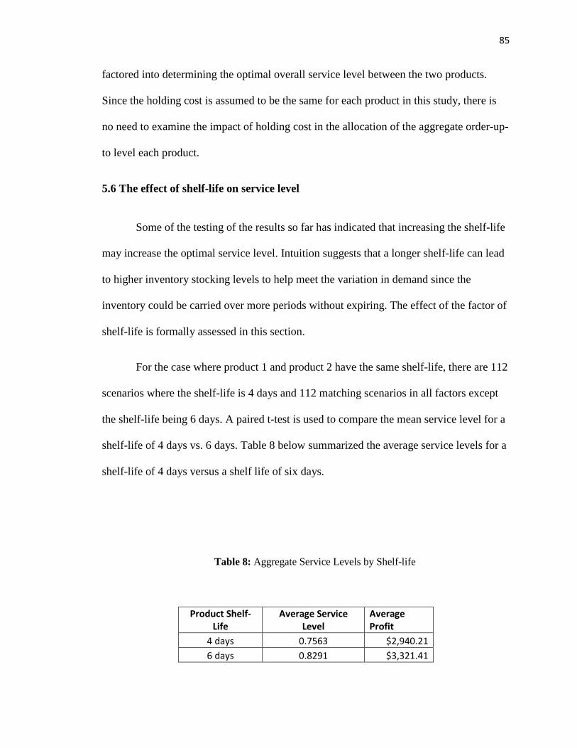
85

factored into determining the optimal overall service level between the two products.

Since the holding cost is assumed to be the same for each product in this study, there is

no need to examine the impact of holding cost in the allocation of the aggregate order-up-

to level each product.

5.6 The effect of shelf-life on service level

Some of the testing of the results so far has indicated that increasing the shelf-life

may increase the optimal service level. Intuition suggests that a longer shelf-life can lead

to higher inventory stocking levels to help meet the variation in demand since the

inventory could be carried over more periods without expiring. The effect of the factor of

shelf-life is formally assessed in this section.

For the case where product 1 and product 2 have the same shelf-life, there are 112

scenarios where the shelf-life is 4 days and 112 matching scenarios in all factors except

the shelf-life being 6 days. A paired t-test is used to compare the mean service level for a

shelf-life of 4 days vs. 6 days. Table 8 below summarized the average service levels for a

shelf-life of 4 days versus a shelf life of six days.

Product Shelf-Life

Average Service Level

Average Profit

4 days 0.7563 $2,940.21 6 days 0.8291 $3,321.41

Table 8: Aggregate Service Levels by Shelf-life

86

The output from the paired t-test is provided in Appendix D.13. The level of significance

is 1.94 x 10-23 indicating strong evidence that the optimal service level will increase when

the product shelf-life increases. Through the analysis of the effect of substitution in

Section 5.2, it was also shown that shelf-life can play a role in the optimal percentage

allocation of the overall order-up-to level to each product. When one product has a longer

shelf-life than another, it is more advantageous to stock more than the expected market

share of that product. In summary, shelf-life is an important factor for both the

determination of service level and allocation.

5.7 The effect of lead time on service level

Another factor of interest in the simulation optimization study is nonzero lead

time. A comparison can be made in the optimal order-up to levels between the scenarios

where the review period is 3 days and the lead time is 0 vs. the scenarios where the

review period is 2 days with a lead time of 1 day. In both settings, the total cycle length is

3 days, but the introduction of lead time within the coverage period could influence the

optimal inventory policy.

There are 200 paired observations for scenarios involving a review period of 3

days and no lead time versus a review period of 2 days and lead time of 1 day. The

average service levels of the two cases are summarized in Table 9 below.

87

Review period

Lead time

Average Service Level

Average Profit

3 days 0 0.7572 $3,025.70 2 days 1 day 0.8208 $3,153.79

The results of the paired t-test are found in Appendix D.14. With a level of significance

of 5.7 x 10-28, there is strong evidence of an increase in mean service level when going

from no lead time to a lead time of 1 day when the coverage period is fixed at 3 days.

Perhaps this is due to the extra uncertainty of not being able to factor in exactly how

many products will expire during the lead time period when placing an order at the end of

the review period.

5.8 The effect of number of product variants

Finally, the last factor to be analyzed based the results of the simulation-

optimization study is the effect of an increase of number of substitutable variants from 2

to 3. For the n = 3 case, results were only collected for the case where all product variants

have identical properties in terms of unit selling price, unit purchase cost, shelf-life, and

market share. In both the n = 2 and n = 3 cases, the overall market demand is fixed with a

mean of 22 and coefficient of variation of 0.7. Therefore, in the n = 2 case, each variant

Table 9: Aggregate Service Levels by lead time

88

has an expected market share of one-half while in the n = 3 case, each variant gets one-

third of the market share.

The data can be subdivided into the following two cost structure categories:

• Category 1 which involves a unit selling price of $4 for each product and unit

purchase cost of $2

• Category 2 which pertains to a unit selling price of $5 and unit purchase cost of

$1.

There are 48 observations in each category. A paired t-test is employed to analyze the

difference in the average service levels achieved between the n = 2 and n = 3 case within

each cost structure category. Table 10 below summarizes the average service levels for

the n = 2 and n = 3 case for each cost category.

Cost Category

Average service level (n=2)

Avg. Profit (n=2)

Average service level (n=3)

Avg. Profit (n=3)

1 0.6554 $1,876.84 0.6434 $1,877.96 2 0.8828 $4,379.02 0.8917 $4,374.59

The results of the paired t-test are included in Appendices D.15 and D.16. The level of

significance of 0.017 on the paired t-test indicates only a small significant decrease in the

Table 10: Aggregate Service Levels by number of variants for each cost category

89

mean service level when going from two to three products for cost category 1. However,

for cost category 2, the level of significance of 0.037 suggests some evidence that the

service level increases when going from n = 2 to n = 3 products. Thus, there is an

indication that the cost structure interacts with number of product variants. When there is

a low profit margin, increasing the number of products from two to three slightly reduces

the overall service level, perhaps a result of overstocking costs being higher. On the other

hand, when profits are higher relative to overstocking costs, as in the case with cost

category 2, the slight increase in service level when going from two to three products

allows for a higher order-up to level in order to capitalize on higher profit relative to

overstocking costs.

5.9 Summary

The simulation-optimization results and corresponding analysis are useful in

making inference on the true effect of key factors in the determination of optimal

inventory policy under product substitution and perishability. It is clear that factors such

as product substitution, cost structures, shelf-life, and lead time are influential in the

determination of the individual optimal order-up-to levels for two product variants. When

variants have identical properties in terms of cost, market share, and shelf-life, increasing

the number of products available subject to the same market demand could potentially

increase or decrease the required service level depending on the cost structures of the

items under consideration. The results show that when the unit cost is high relative to the

retail price, an increase in the number of variants tends to decrease the aggregate service

level, while the opposite effect seems to occur when the unit cost is low relative to the

retail price.

90

One of the major contributions of this thesis is likely to be the development of a

heuristic approach for determining an acceptable inventory policy for the case of two

product variants. The results of the simulation-study are useful in gaining insight into the

influential factors that need to be included in the heuristic. Although only a limited range

of parameter values were covered in the simulation-optimization study, it is important

that the heuristic performs well under a wider variety of operating conditions. The next

chapter will outline the heuristic development process and an evaluation of its

effectiveness and robustness.

91

Chapter 6: Heuristic Development and Performance

6.1 Overview

Based on the results of the simulation-optimization study, a heuristic is developed

and tested for the case of two products under product substitution and perishability for an

(R,Si) system. Heuristics can provide good, relatively quick solutions to complex

problems when time and technology are limited in order to find the true global optimal

solution. Typically for the case of perishable products, the standard newsvendor model is

used as an approximate solution in cases where the shelf-life of the product extends

beyond the cycle length (Van Donselaar 2006). An approach that takes into account

factors such as substitution, shelf-life, lead time, etc. should enhance the effectiveness of

the heuristic.

The organization of this chapter is as follows. Section 6.2 shows the development

of the heuristic approach for the two product case. Section 6.3 deals with the performance

of the heuristic and finally, Section 6.4 is a summary of the chapter.

6.2 Heuristic Development

The basic idea behind the development of a heuristic for an (R,Si) system under

product substitution and perishability is to provide a solution that expands on the

concepts of the newsvendor model. As discussed in Chapter 3, the newsvendor model is a

special case of this perishability problem where the shelf-life of the products is equal to

92

the coverage period when lead time is zero. However, adding the factors of increased

shelf-life, product-based substitution, and age-based substitution make the problem much

more complex. In the newsvendor model, the optimal order-up-to level is dependent on

the cycle service level which is a ratio of the costs of understocking to the total costs of

understocking and overstocking costs. Even in this extended case, inventory managers

should make decisions by making appropriate trade-offs between understocking and

overstocking costs as in the newsvendor model.

As mentioned in Chapter 5, the determination of inventory policy for an (R,Si)

system for two products can be broken down into two components. The first component

is the determination of the aggregate order-up-to level of the two product variants and

then the second component is how the aggregate order-up-to level will be allocated to

each product. A separate heuristic will be developed for each component and then

combined to provide a solution for S1 and S2.

The fundamental idea behind the first component of the determination of S1 and

S2 is that the aggregate order-up-to level pertains to the overall market demand. Under

product substitution, partial inventory pooling takes place where a proportion of excess

inventory of one product can potentially be met by demand of the substitute product in

the event of a stockout of that product. The substitution effect as well as effects from

additional factors such as cost structure, shelf-life, and lead time can impact the optimal

aggregate order-up-to level from the two products. Therefore, as in the newsvendor

model, a ratio of understocking costs to overstocking costs can be developed for this

extended case where two products are under consideration with additional factors. Let ST

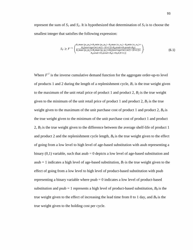
93

represent the sum of S1 and S2. It is hypothesized that determination of ST is to choose the

smallest integer that satisfies the following expression:

Where F-1 is the inverse cumulative demand function for the aggregate order-up-to level

of products 1 and 2 during the length of a replenishment cycle, B1 is the true weight given

to the maximum of the unit retail price of product 1 and product 2, B2 is the true weight

given to the minimum of the unit retail price of product 1 and product 2, B3 is the true

weight given to the maximum of the unit purchase cost of product 1 and product 2, B4 is

the true weight given to the minimum of the unit purchase cost of product 1 and product

2, B5 is the true weight given to the difference between the average shelf-life of product 1

and product 2 and the replenishment cycle length, B6 is the true weight given to the effect

of going from a low level to high level of age-based substitution with asub representing a

binary (0,1) variable, such that asub = 0 depicts a low level of age-based substitution and

asub = 1 indicates a high level of age-based substitution, B7 is the true weight given to the

effect of going from a low level to high level of product-based substitution with psub

representing a binary variable where psub = 0 indicates a low level of product-based

substitution and psub = 1 represents a high level of product-based substitution, B8 is the

true weight given to the effect of increasing the lead time from 0 to 1 day, and B9 is the

true weight given to the holding cost per cycle.

(6.1)

94

The motivation for Equation 6.1 in part stems from observations of the

simulation-optimization study discussed in Chapter 5. As mentioned earlier, the concept

behind the ratio in the right-hand side of equation 6.1 is based on the newsvendor model

where the CSL is the ratio of the marginal understocking cost to the sum of the marginal

understocking and overstocking costs. Through the simulation-optimization study, we

are able to gain some insights on how some key factors impact the service level in

maximizing expected profit. It is confirmed that cost structure plays an important role in

the determination of mean service level for two substitutable and perishable items. In the

standard newsvendor model, one fundamental understocking cost is the profit margin

defined as the retail price minus the unit cost. In this case of two products, there are two

retail prices and unit costs; therefore, distinctions are made between what are the

maximum and minimum retail prices and unit costs respectively. The numerator of the

ratio in the right-hand side of Equation 6.1 includes the differentials of the retail prices

multiplied by the weights B1 and B2 and the unit costs, multiplied by the weights B3 and

B4. However, the denominator only includes the retail prices since the unit costs are

canceled out by the fact that in the absence of salvage value the unit cost is the

overstocking cost. One factor included in the denominator but not the numerator is the

holding cost. The holding cost is multiplied by the weight B9 and the coverage period

(R+L) which represents the marginal holding cost per coverage period. This step is

necessary so that the same weight can be applied to problems under all types of operating

conditions where the coverage period can vary.

Other factors incorporated into the ratio in the right-hand side of Equation 6.1

include age-based substitution (asub), product-based substitution (psub), and lead time,

95

L. Based on the results of the simulation-optimization study, it is shown that these factors

can be influential in the determination of service level. Therefore, these factors are

applied to both numerator and the denominator and are multiplied by the weights, B6, B7,

and B8 respectively.

The next step in the development of the first component of the heuristic is to

determine good estimates for B1, B2, …, B9. Let b1, b2, …, b9 represent single point

estimate for the parameters B1, B2, …, B9. The least-squares method can be used to find

b1, b2,…b9 based on the minimization of the squared error between the simulated-optimal

solutions and the forecasted solution from (6.1). The 600 observations from the

simulation-optimization study, only cover a limited range of parameter values. Therefore,

a new set of data was generated randomly with varying parameter values. A set of 30 new

observations were generated by selecting scenarios that come from the following

parameter ranges:

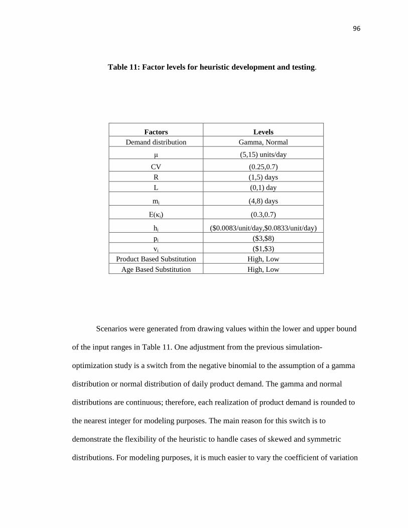
96

Factors Levels Demand distribution Gamma, Normal

μ (5,15) units/day

CV (0.25,0.7) R (1,5) days L (0,1) day

mi (4,8) days

E(κi) (0.3,0.7)

hi ($0.0083/unit/day,$0.0833/unit/day) pi ($3,$8) vi ($1,$3)

Product Based Substitution High, Low Age Based Substitution High, Low

Scenarios were generated from drawing values within the lower and upper bound

of the input ranges in Table 11. One adjustment from the previous simulation-

optimization study is a switch from the negative binomial to the assumption of a gamma

distribution or normal distribution of daily product demand. The gamma and normal

distributions are continuous; therefore, each realization of product demand is rounded to

the nearest integer for modeling purposes. The main reason for this switch is to

demonstrate the flexibility of the heuristic to handle cases of skewed and symmetric

distributions. For modeling purposes, it is much easier to vary the coefficient of variation

Table 11: Factor levels for heuristic development and testing.

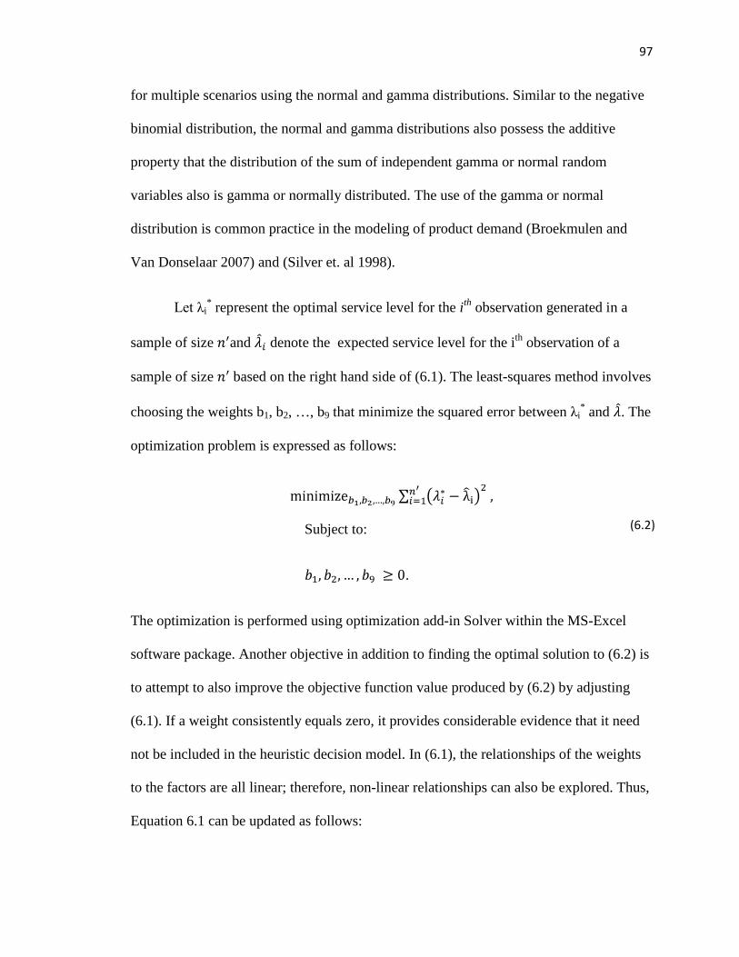
97

for multiple scenarios using the normal and gamma distributions. Similar to the negative

binomial distribution, the normal and gamma distributions also possess the additive

property that the distribution of the sum of independent gamma or normal random

variables also is gamma or normally distributed. The use of the gamma or normal

distribution is common practice in the modeling of product demand (Broekmulen and

Van Donselaar 2007) and (Silver et. al 1998).

Let λi* represent the optimal service level for the ith observation generated in a

sample of size and denote the expected service level for the ith observation of a

sample of size based on the right hand side of (6.1). The least-squares method involves

choosing the weights b1, b2, …, b9 that minimize the squared error between λi* and . The

optimization problem is expressed as follows:

Subject to:

.

The optimization is performed using optimization add-in Solver within the MS-Excel

software package. Another objective in addition to finding the optimal solution to (6.2) is

to attempt to also improve the objective function value produced by (6.2) by adjusting

(6.1). If a weight consistently equals zero, it provides considerable evidence that it need

not be included in the heuristic decision model. In (6.1), the relationships of the weights

to the factors are all linear; therefore, non-linear relationships can also be explored. Thus,

Equation 6.1 can be updated as follows:

(6.2)

98

.

The total number of decision variables as been reduced from 9 to 7 as the weights for

product-based substitution and maximum price equal zero consistently in the

optimization trials. Based on the results of the simulation-optimization study, the effect of

product-based substitution on average service level is very weak; therefore, it is no

surprise that the weight of the coefficient B5 turns out to be zero. For the shelf-life term,

an exponential fit seems to work better than the linear fit, therefore the weight, B4 is an

exponent applied to the difference of the average shelf-life of the two products and the

replenishment cycle length. For the age-based substitution and lead time, it appears that

there is an interaction with the cost properties such that for a higher profit margin relative

to the overall costs, the effects of age-based substitution and lead time increases. Another

interaction seemed to be present with the holding cost. If the holding cost is higher

relative to the average profit margin, then the effect of the holding cost factor is markedly

enhanced.

The next step in the heuristic development is to provide a good approximation of

the optimal allocation of ST to each product. Let ψi* represent the optimal percentage

allocation of ST to product 1 and denote the predicted percentage allocation of ST to

product 1. Based on the simulation-optimization study, it is believed that cost

differentials, shelf-life differentials, product-based substitution, and possible interactions

(6.3)

99

among these factors play the most significant roles in the allocation of the overall sum of

the order-up-to levels. Since age-based substitution only had a slight conditional impact

on the optimal allocation, it will not be included in the heuristic. As a first step, can

be expressed as follows:

Where E(κ) is the expected market share the designated product 1, ϑ1 is the true weight

for the unit purchase cost difference between product 1 and product2, ϑ2 is the true

weight for the shelf-life difference between product 1 and product 2, ϑ3 is the true weight

for the interaction of product-based substitution and the unit cost differential, and ϑ4 is

the true weight of the interaction of shelf-life differential and product based substitution.

Equation (6.4) needs to be adjusted depending on the value of the E(κ) term based

on observations from the simulation optimization study. For example, if the E(κ) equals

0.3 and ψi* indicates an increase in the percentage allocation from the expected market

share, then that increase is larger than if E(κ) were 0.7 since E(κ) has a maximum at 1. By

the same token, if E(κ) = 0.3 and ψi* indicates a decrease in the expected market share,

then the magnitude of the decrease is smaller than if E(κ) = 0.7 since E(κ) has a minimum

value of 0. Let φi be the value obtained by the following expression:

The value obtained for φi is used in determining which can be expressed as:

(6.4)

(6.5)

(6.6)

100

where ϑ5 is the true weight given to how the percentage allocation of the overall sum of

the order-up-to levels of both products changes with respect to the expected market share

of product 1. The parameters ϑ1, ϑ2, ϑ3, ϑ4, and ϑ5 can be estimated through the least-

squares method of minimizing the squared error between ψi* and . Let c1, c2, c3, c4,

and c5 be point estimates of the parameters ϑ1, ϑ2, ϑ3, ϑ4, and ϑ5. The unconstrained

minimization problem under the least squares method is as follows:

A training sample of n = 30 observations are used to find c1, c2, c3, c4, and c5 through MS

Excel/Solver. The parameters values are randomly selected based on the ranges defined

in Table 11. The solver optimization routine indicates that a solution is found once

optimality conditions are satisfied. Overall, the estimated weights for both the

determination of and are summarized respectively in Table 12 and Table 13 below:

(6.7)

101

Estimated Weight Value

b1 3.29

b2 1.70

b3 3.52

b4 3.00

b5 6.14

b6 11.93

b7 0.15

Estimated Weight Value

c1 -1.00

c2 1.47

c3 -1.32

c4 2.05

c5 0.24

Table 12: Estimated weights for determining the predicted service level of the combined order-up-to levels of two products.

Table 13: Estimated weights for determining the predicted allocation of overall order-up-to level for 2 products.

102

With the estimates of the weights listed in Tables 6.2 and 6.3, the combined heuristic

approach is now complete. Let and be the predicted order-up-to levels for products

1 and 2 in a (R,Si) system under product substitution and perishability. and are

determining by Algorithm 6.1 outlined below:

Algorithm 6.1:

1. Find ST using Equation (6.3) along with the estimated weights from Table 6.2

2. Determine using Equation (6.6) along with estimated weights from Table 6.3.

3. Multiply ST by and round to the nearest integer to find .

4. Find by subtracting from ST: = ST -

This combined heuristic approach will be referred to as the Extended Newsvendor

(ENVR) heuristic. The next step is to test how well the ENVR heuristic performs under

changing operating conditions.

6.3 Performance of Heuristics

In order to evaluate the proposed heuristic, the expected profit obtained by the

above heuristic can be compared to the expected profit obtained from the simulated-

optimal solution. In order to provide a frame of reference on the performance, a standard

newsvendor (NVR) heuristic will also be used in a comparative study. The NVR heuristic

is summarized in Algorithm 6.2 below:

Algorithm 6.2

1. Set and find ST based on the Equation 6.3.

103

2. Set = E(κ)

3. Multiply ST by and round to the nearest integer to find .

4. Find by subtracting from ST.

Appendix E.1 contains the detailed results of 100 scenarios that were generated from the

parameters listed in Table 11. For each scenario, an exhaustive search was performed

among the candidate S1 and S2 solutions, in order to find the simulated-optimal solution.

Small values for mean daily demand were selected in order for quickening the exhaustive

search to be executed. Of the 100 scenarios, 65 assume a gamma distribution for daily

demand, and 35 assume a normal distribution. For the gamma distribution, the coefficient

of variation of demand is arbitrarily selected between 0.4 and 0.7 while with the normal

distribution, the coefficient of variation of demand is arbitrarily selected between 0.3 and

0.35, in order to reduce the probability of negative realizations of daily demand. Most

other parameter values are randomly chosen among the ranges listed in Table 11, while

assuming that the shelf life of each product exceeds the coverage period. For the mean

daily demand, the values are arbitrarily chosen, but varying between the same ranges

listed in Table 11. All together, the 100 scenarios form a set that spans a wide range of

operating conditions.

For each of the 100 scenarios, both the ENVR and NVR heuristics are used to

obtain solutions for S1 and S2. The ENVR and NVR solutions are evaluated through

simulation and the expected profit obtained from each is compared to that produced by

the simulated-optimal solution. The number of replications required for each simulation

run varies according to how many replications are necessary to guarantee that the

104

sampling error is within 2% of the true expected profit. This feature can easily be

implemented using OptQuest. Therefore, the number of replications will vary among the

different scenarios based on the coefficient of variation of demand and also between each

type of method used (Simulated optimal, ENVR, or NVR) in determining S1 and S2. It is

possible that the heuristics could produce a solution that is equal to the simulated-optimal

solution, or yield a mean profit that is so close to the mean profit produced by the

simulated-optimal solution that the difference may be statistically insignificant.

Some of the parameters that were previously fixed will be allowed to vary for the

testing of the heuristic decision rule. For the substitution parameters, the level of both

product-based and age-based substitution will vary between high and low, however, the

parameters α, β, ω, γ, and δ will be allowed to vary more so than allowed in the

simulation-optimization study. For example, in the simulation-optimization study, the

substitution scenario of high product-based and high age-based substitution implied α =

0.5, β = 0.4, ω = 0.8, γ = 0.8, and δ = 0.7. For testing the heuristic under a high-high

substitution scenario, each of these parameters will vary in order to incorporate the

uncertainty of these parameters. The same idea applies to the variance of the market share

for each product. For the simulation-optimization study, the market share for each

product were based on a uniform distribution with a lower bound equal to the expected

market share less 0.2, and the upper bound being the expected market share plus 0.2. The

width of this region still will not exceed 0.4, but will vary between 0.2 and 0.4.

The results from the 100 scenarios generated are contained in Appendix E.2. The

ENVR heuristic performs very well compared to the NVR heuristic. Table 14 below

gives some numerical measures of the performance of each heuristic.

105

Table 14: Summary of the performance of each heuristic

Heuristic

Average Decrease from

Simulated-Optimal Solution

Profit

Maximum Decrease from Simulated-Optimal

Solution Profit

Standard Deviation of Differential

# of scenarios equal to

simulated optimal solution

ENVR 0.59% 3.50% 0.60% 14 NVR 2.02% 11.70% 2.53% 3

The mean profit obtained from the ENVR heuristic has only a 0.59% average decrease

from the simulated-optimal mean profit with a standard deviation of 0.60% while the

average decrease in mean profit for the NVR heuristic was 2.02% with a standard

deviation of 2.53%. The heuristic solution matches the simulated optimal solution in 14

out of the 100 scenarios for the ENVR heuristic compared to just 3 for the NVR heuristic.

The worse case performance for the ENVR heuristic is a 3.5% decrease in mean profit

compared to a 11.7% decrease resulting from the NVR heuristic.

A two sample t-test assuming unequal variances can be applied for each scenario

to determine if there is a truly significant optimality gap between the heuristic solution

and simulated-optimal solution. The results of the t-test are contained in Appendix E.3.

106

Overall, there were only 3 scenarios where the simulated-optimal solution was

statistically better than the ENVR heuristic while there were 32 scenarios where the

where the simulated-optimal solution was statistically better than the NVR heuristic.

Thus it can be concluded that the ENVR tends to outperform the NVR heuristic. There is

no clear pattern on the conditions where either the ENVR or NVR heuristic perform

poorly. Although the NVR heuristic performs fairly well in some cases, it is not

recommended as a whole, since it has shown to often yield an expected profit

significantly lower than the simulated-optimal solution. It is unclear as to the exact

operating conditions under which decline in expected profit can be expected. Since the

ENVR heuristic appears to perform better and incorporates more factors than the NVR

heuristic, it is the obvious better choice among the two alternatives.

6.4 Summary

The ENVR heuristic appears to perform very well based on the parameter value

ranges outlined in Table 11. Thus, for two perishable items of 8 days or less, review

periods between 1 and 5 days, and lead times of either 0 or 1 day, the ENVR heuristic can

be safely applied. There should be some understanding of the nature of product-based and

age-based substitution such that it can be categorized as either high or low for the

particular application. It is important to be able to have accurate knowledge of the daily

product demand parameters. The ENVR decision rule developed here heuristic has

demonstrated flexibility in being applicable for two types of demand distributions, one

skewed and the other symmetric. Thus, it is likely to be effective under other types of

distributions.

107

With the aid of the ENVR heuristic, practitioners can quickly generate good

solutions to complex problems involving managing two product variants under an (R,Si)

system with product substitution and perishability. Although having the tool of

simulation-optimization should guarantee good results, it may not be feasible to

implement the technology in many real world applications with limited resources. There

are significant time and monetary savings in using the ENVR heurstic compared to a

simulation-optimization model. The ENVR heuristic performs well under the range of

parameter values used in Table 11; however, there is no guarantee of the same success

under a more expansive range of parameter values. Therefore, practitioners must use

caution when applying the heuristic to parameter values outside the range in Table 11.

108

Chapter 7: Conclusion and Future Research

7.1 Conclusion

In conclusion, this thesis has provided new insights into an (R,Si) inventory

control system under product substitution and perishability. A thorough review of the

literature relating to inventory policy and product substitution and perishability revealed a

gap in the body of knowledge, i.e. analysis of the simultaneous effects of product

substitution and perishability. Prior studies did not attempt to combine the concepts of

both product-based substitution and age-based substitution and how they play a joint role

in the determination of an appropriate perishable inventory control policy. In this thesis,

new insights are gained on the combined topic of product substitution and perishability

through the tool of simulation-optimization, which is used to analyze a complex

inventory problem that is difficult to solve analytically. A carefully designed simulation-

optimization study under varying operating conditions enabled further analysis of the

impact of key factors such as shelf-life, cost structures, substitution characteristics, lead-

time, and number of products on optimal inventory policy for maximizing expected

profit.

The information gained from the results of the simulation-optimization study were

utilized in developing a heuristic decision rule for the two product variants case. A two

pronged approach is used in establishing the order-up-to levels of the two variants. The

first component involves determining the aggregate order-up-to level of the two variants

109

and the second component deals with the appropriate allocation of the aggregate order-

up-to level to determine the exact order-up-to levels of each product. The underlying idea

behind the heuristic developed is to build on and embellish the concepts of the traditional

newsvendor model. The newsvendor model involves deriving the service level based on

the relative values of the marginal overstocking vs. understocking costs. Since the general

(R,Si) model involves more factors that the standard newsvendor approach, these factors

needed to be incorporated into the suggested heuristic technique. This heuristic uses a

two step approach in determining the respective order-up-to levels of two products that is

based on the respective impacts of the key factors of substitution, cost properties, shelf-

life, and lead time.

Based on the results of the simulation-optimization study and performance of the

ENVR system, there is now a new understanding of how the factors of shelf-life, cost

properties, lead time, and number of products influence inventory policy in maximizing

expected profit under an (R,Si) system with product substitution and perishability. The

main conclusions from the simulation-optimization study are summarized as follows:

1) An increased shelf-life tends to drive up the order-up-to level for a particular

product. Differentials in shelf-lives between two products are likely to alter the

allocation of the aggregate order-up-to level compared to the expected market

share of each product.

2) Cost structures are also very influential in both the determination of aggregate

order-up-to level and its allocation among the product variants. When marginal

profit is high relative to overall costs, the items’ order-up-to levels tend to

110

increase. When all other factors are constant, an increase in holding cost appears

to decrease order-up-to levels.

3) For the allocation of overall order-up-to level to each product, the only important

cost properties are differentials in unit purchase costs. The balance seems to tilt in

favor of products with lower unit purchase costs since product expiration is less

costly.

4) Product-based substitution does not play a significant role in the determination of

aggregate order-up-to level which appears to be intuitive; however, it seems to be

significant in the allocation of the aggregate order-up-to level to each product.

5) Age-based substitution tends to play a significant role in the determination of the

aggregate order-up-to level, but not the allocation of the aggregate order-up-to

level to each product.

6) There is evidence that the existence of lead time can increase the order-up-to

levels relative to a fixed length coverage with no lead time. This study explored

the case of a review period of 2 days and lead time of 1 day vs. the case of a

review period of 3 days and 0 lead time.

7) There seems to be a slight significant difference in the aggregate order-up-to level

when going from two product variants to three product variants. The difference in

service levels between the two and three product variant case prove to be

dependent on the cost structures of the products. When profit margins are lower

relative to overall costs, increasing the number of products from two to three

tends to lead to a slight reduction in overall mean service level. When profit

111

margins are high relative to overall costs, increasing the number of products from

two to three leads to a slight increase in overall mean service level.

8) Going from a low to a high level of both product-based and age-based substitution

increases expected profits. A customer’s willingness to substitute leads to more

sales relative to a fixed amount of inventory available.

All together, the information gained from the simulation-optimization study is helpful in

the development of a heuristic decision rule for the two product variant case.

The proposed extended newsvendor (ENVR) heuristic decision rule is tested under a

variety of operating conditions spanning a wide range of parameter values for the factors

involved in the problem. The ENVR heuristic is compared to the simulated-optimal

approach and also to a standard newsvendor (NVR) heuristic that only incorporates some

cost properties. The ENVR heuristic outperforms the NVR heuristic, and appears to be

statistically on par with the simulation-optimization methodology solution in 97 of the

100 scenarios. On the other hand, the NVR heuristic only produces a solution with no

apparent statistical difference in expected profit in only 67 of the 100 scenarios. The

overall average loss in expected profit between the ENVR solution and simulated-optimal

solution is only 0.59% compared to 2.02% for the NVR heuristic. Thus, there is good

evidence that the ENVR is a well-performing heuristic that can provide near-optimal

inventory policy in expected profit maximization for an (R,Si) system under product

substitution and perishability. Practitioners can safely apply ENVR heuristic to problems

under similar parameter value ranges explored in this study, but should take caution in

going beyond those ranges. Future research will be focused on the sensitivity of the

heuristic beyond the parameter ranges selected in this study.

112

The findings from this thesis serve as a contribution to both the academic

literature on inventory pertaining to product substitution and perishability and as an aid to

practitioners. The previously existing gap in literature that combines product substitution

and perishability has been addressed with this thesis which provides detailed analysis

from the case of two perishable product variants and a partial exploration into the case of

three variants. This thesis has also touched on an extension of the nature of substitution

that extends beyond the product-based case under a stockout of a preferred product to the

situation where a customer could incorporate product age properties into their

substitution decisions. In most of the literature pertaining to substitution, it is assumed

that utility is independent of the remaining shelf-life of the product. In this study, there is

a distinction made between fresh and old items. Customers are assumed to get the most

utility out of fresher products; therefore, they are likely to choose fresh products first, and

if the fresh version of their preferred product is out of stock, they face a decision that

could involve switching to another product, or an older version of the same product. As

proven by the analysis done in this study, both types of substitution can play a major role

in determining appropriate inventory policies. Practitioners needs are also addressed

through an understanding of the key factors that influence inventory policy for an (R,Si)

system, but more specifically with the proposed ENVR heuristic that can yield a quick,

and a near-optimal solution to a complex problem involving two perishable product

variants.

7.2 Future Research

Although much work is accomplished in this study, there are identifiable areas for

potential future research. One such future direction would be to develop a heuristic that

113

can deal more than two product variants and also perform well under an even more

expanded range of parameter values. Based on the methodology followed in this thesis,

the process of analyzing more than two product variants grows exponentially in time for

each additional product considered. Introducing an additional product introduces an

additional decision variable for the simulation-optimization problem which in turn

enlarges the solution space. More time is required to do such an expanded study for

multiple products. Nevertheless, the insights gained from 2 products provide a good

preliminary step.

A second area of future research is to explore other objectives besides profit

maximization. Other studies relating to perishable inventory explore objectives such as

maximizing product freshness, minimizing the number of stockouts, or minimizing the

number of discarded items. A future study could involve exclusively looking into either

one of these objectives, or using a multi-objective approach when all these objectives are

considered simultaneously.

Another possible research direction is to employ more considerations of multi-

echelon supply chains into the decision-making. The study in this thesis assumed that the

retailer can dictate the exact order-up-to level for each product. Many food products

operate under Vendor-Managed systems where suppliers have more control in setting

inventory policy. Therefore, one such study can be a comparison of VMI versus RMI

supply chains. Prior research has shown that alternate supply-chain configurations can

impact the optimal inventory policy for the supply chain. To our knowledge, no previous

studies have analyzed VMI and RMI supply chain under both product substitution and

perishability.

114

Another future research direction is to explore other scenarios regarding product

demand. One situation is price-dependent demand where price markdowns are created for

perishable goods as they near the end of their shelf-lives. Although the notion of

decreasingly product utility is factored into the models in this thesis, it is done so through

decreasing the probability of substitution. Another option is to explore the effect of stock-

level based demand on inventory policy. There is evidence that the customer’s inclination

to purchase may be affected by the level of inventory available.

This thesis assumed an (R,Si) system of control where only the order-up-to level Si

is considered as a decision variable. Future studies should treat the review period R as a

decision variable and seek to achieve joint optimization of R and Si. In addition, this

system of inventory control could be modified into a can-order (R,si,Si) system where an

order is placed only if the inventory position reaches the level si for each product.

Another possibility is to switch the assumption from a periodic review system to a

continuous review system where inventory is monitored according to an (si,Si) system

where an order is placed automatically once the inventory position reaches the level of si.

Finally, future research can look to incorporate constraints such as shelf-space and

load capacity on orders, and also go beyond just one product class. Practitioners are

typically faced with such constraints and handling multiple product classes. Therefore,

heuristics can be developed that deal with these types of situations.

Overall, the topic of inventory management involving product substitution and

perishability appears to be rich in terms of future research due to the current gaps in

existing literature. It is hoped that this thesis is able to fill in some of the gaps in the

115

extant literature. More work nevertheless needs to be done to gain a comprehensive

understanding of the topic. With more available literature in this area, practitioners in the

food industry and beyond will be provided with better guidelines to alleviate current

problems faced in managing perishable inventories.

116

List of References

Aras, N., V. Verter, T. Boyaci. Coordination and priority decisions in hybrid manufacturing/remanufacturing systems. Production and Operations Management 2006; 15(4): 528-543 Baird, N. Creating competitive advantage with service parts logistics. Inbound Logistics 2004 (April) Bassok, Y., R. Anupindi, R. Akella, Single-period multi-product inventory model with substitution. Operations Research 1999; 47(4): 632-642 Benjaafar, S., W. Cooper., J. Kim. On the benefit of inventory pooling in production-inventory systems. Management Science 2005; 51: 548-565 Broekmeulen, R., K, van Donselaar. A replenishment policy for a perishable inventory system based on estimated aging retrieval behavior. Working paper, Technische Universiteit Eindhoven, Eindhoven, The Netherlands Campo, K., E. Gijsbrechts, P. Nisol. Towards understanding consumer response to stockouts. Journal of Retailing 2000; 76(2): 319-242 Chapman, J.F., C. Hyam, and R. Hick. Blood Inventory Management Vox Sanguinis 2004; 87(2): 143-145. Chazan, D., and S. Gal. A Markovian Model for a Perishable Product Inventory.Management Science 1977; 23(5): 512-521 Chen, L., E.L. Plambeck. Dynamic inventory management with learning about the demand distribution and substitution probability. Manufacturing & Service Operations Management 2008; 10(2): 236-256 Chiu, H.N. A heuristic (R,T) periodic review perishable inventory model with lead times. International Journal of Productions Economics 1995; 42: 1-15 Chopra, S., M. Sodhi. Managing risk to avoid supply chain breakdown. Sloan Management Review 2004; 46: 53-61. Cohen MA. Analysis of single critical number ordering policies for perishable inventories. Operations Research 1976; 24(4): 726-741.

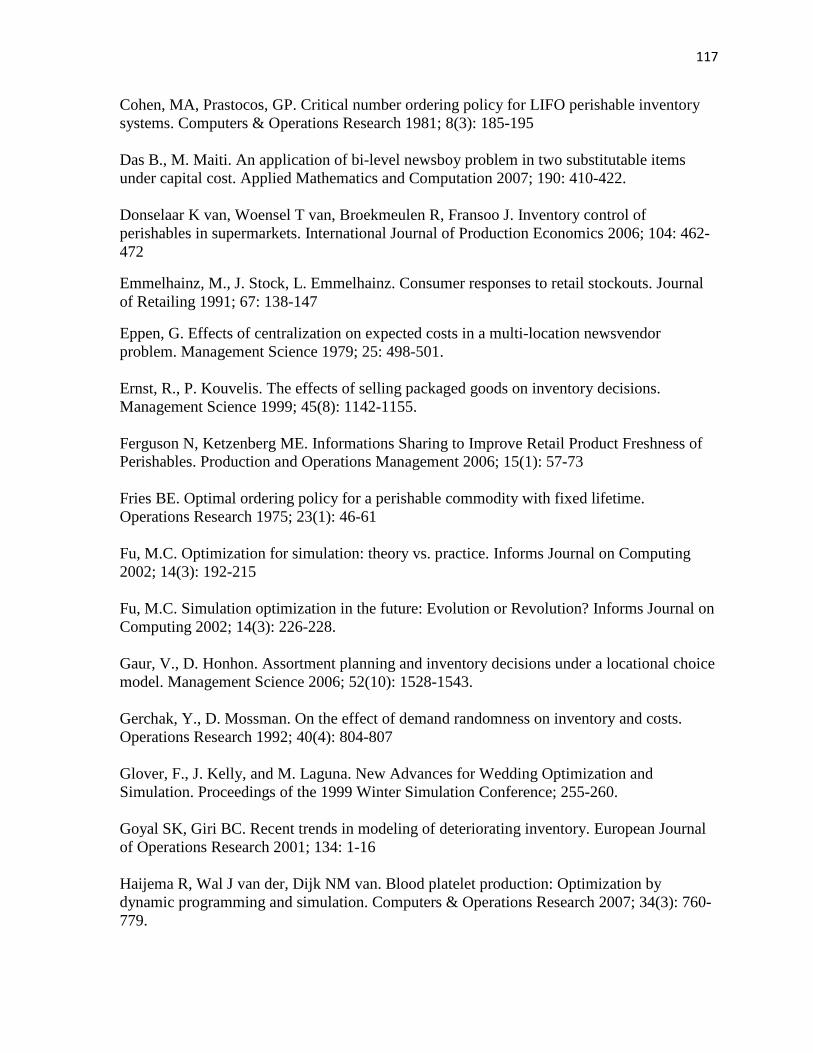
117

Cohen, MA, Prastocos, GP. Critical number ordering policy for LIFO perishable inventory systems. Computers & Operations Research 1981; 8(3): 185-195 Das B., M. Maiti. An application of bi-level newsboy problem in two substitutable items under capital cost. Applied Mathematics and Computation 2007; 190: 410-422. Donselaar K van, Woensel T van, Broekmeulen R, Fransoo J. Inventory control of perishables in supermarkets. International Journal of Production Economics 2006; 104: 462-472

Emmelhainz, M., J. Stock, L. Emmelhainz. Consumer responses to retail stockouts. Journal of Retailing 1991; 67: 138-147

Eppen, G. Effects of centralization on expected costs in a multi-location newsvendor problem. Management Science 1979; 25: 498-501. Ernst, R., P. Kouvelis. The effects of selling packaged goods on inventory decisions. Management Science 1999; 45(8): 1142-1155. Ferguson N, Ketzenberg ME. Informations Sharing to Improve Retail Product Freshness of Perishables. Production and Operations Management 2006; 15(1): 57-73 Fries BE. Optimal ordering policy for a perishable commodity with fixed lifetime. Operations Research 1975; 23(1): 46-61 Fu, M.C. Optimization for simulation: theory vs. practice. Informs Journal on Computing 2002; 14(3): 192-215 Fu, M.C. Simulation optimization in the future: Evolution or Revolution? Informs Journal on Computing 2002; 14(3): 226-228. Gaur, V., D. Honhon. Assortment planning and inventory decisions under a locational choice model. Management Science 2006; 52(10): 1528-1543. Gerchak, Y., D. Mossman. On the effect of demand randomness on inventory and costs. Operations Research 1992; 40(4): 804-807 Glover, F., J. Kelly, and M. Laguna. New Advances for Wedding Optimization and Simulation. Proceedings of the 1999 Winter Simulation Conference; 255-260. Goyal SK, Giri BC. Recent trends in modeling of deteriorating inventory. European Journal of Operations Research 2001; 134: 1-16 Haijema R, Wal J van der, Dijk NM van. Blood platelet production: Optimization by dynamic programming and simulation. Computers & Operations Research 2007; 34(3): 760-779.

118

Heller, T. Sales grow so does competition. Progressive Grocer 2002 81(10) 103-106.

Ketzenberg, M. Information in Supply Chain Management of Perishables. PhD. Dissertation, University of North Carolina, Chapel Hill, 2000. Khouja M., A. Mehrez, G. Rabinowitz. A two-item newsboy problem with substitutability. International Journal of Production Economics 1996; 44: 267-275 Kök, A.G. Management of product variety in retail operations. PhD. Dissertation, University of Pennsylvania, Philadelphia, PA, 2003. Kök, A.G., M. Fisher. Demand estimation and assortment optimization under substitution: methodology and application. Operations Research 2007; 55(6): 1001-1021 Kraiselburd, S., Narayanan, V.G., and Raman, A. Contracting in a supply chain with stochastic demand and substitute products. Production and Operations Management 2004; 13(1): 46-62 Law AM, Kelton WD. Simulation modeling and analysis (third ed.). Boston: McGraw-Hill, 2000. Law, A., M. McComas. Simulation-based optimization. In Proceedings of the 2000 Winter Simulation Conference, ed. J Joines, R. Barton, K. Kang, and F. Fishwick, 46-49. Institute of Electival and Electronics Engineers. Levine, D.M, D.F. Stephan, T.C Krehbiel, M.L. Berenson. Statistics for Managers Using Microsoft Excel. 5th Edition. Pearson Prentice Hall, Upper Saddle River, New Jersey, 2008: 422-434. Lodree, E.J., C.D. Geiger. A simulation optimization approach for the two product newsvendor problem. Society for Modeling and Simulation Advanced Simulation Technologies Conference Proceedings, Orlando, FL, 2003. Mahajan, S., G.J. van Ryzin. . Stocking retail assortments under dynamic consumer substitution. Operations Research 2001. 49(3): 334-351 McGillivray, A.,E.A. Silver. 1978. Some concepts for inventory control under substitutable demand. INFOR 16(1) 47-63 Mishra, B.K., S. Raghunathan. Retailer vs. vendor-managed inventory and brand competition. Management Science 2004; 50(4): 445-457. Nagarajan, M., S. Rajagopalan. Inventory models for substitutable products: optimal policies and heuristics. Management Science 2008; 54(8): 1453-1466

119

Nahmias S. Optimal ordering policies for perishable inventory – II. Operations Research 1975;23(4):735-749. Nahmias S. Perishable inventory theory: a review. Operations Research 1982; 30(4): 680-708

Netessine, S., N. Rudi. Centralized and competitive inventory models with demand substitution. Operations Research 2003; 51(2): 329-335. Parlar, M. Optimal ordering policies for a perishable and substitutable product—A Markov decision model. INFOR 23: 182-195. Pasternack, B., Z. Drezner. Optimal inventory policies for substitutable commodities with stochastic demand. Naval Research Logistics 1991 38(2): 221-240. Raafat F. Survey of literature on continuously deteriorating inventory. Journal of Operations Research Society 1991;42: 27-37. Rajaram, K.C., S. Tang. The impact of product substitution on retail merchandising. European Journal of Operations Research 2001; 135(3): 582-601. Reyes P.M. Integrating the effects of product substitution and proliferation into grocery supply chain decisions. PhD. Dissertation. The University of Texas at Arlington, Arlington Texas, 2002. Schary, P.B., M. Christopher. The Anatomy of a Stock-Out. Journal of Retailing 1979; 55(2): 59-70 Singh, V.P., S.K. Jain, and A. Tyagi. Risk and Reliability Analysis: A Handbook for Civil and Environmental Engineers. ASCE Press, 163. Silver EA, Pyke DF, Peterson R. Inventory Management and Production Planning and Scheduling (third ed.). Chichester: Wiley, 1998. Smith, S.A., N. Agrawal. Management of multi-item retail inventory Systems with demand substitution. Operations Research 2000; 48(1): 50-64. Strijbosch, L.W.G., J.J.A. Moors. The impact of unknown parameters on (R,S)-inventory control performance. European Journal of Operations Research 2005; 162: 805-815. Strijbosch, L.W.G., J.J.A. Moors. Modified normal demand distributions in (R,S)-inventory control. European Journal of Operations Research 2006; 172: 201-212. Tarim, S.A., B.G. Kingsman. Modeling and computing policies for inventory systems with non-stationary stochastic demand. European Journal of Operations Research 2006; 174: 581-599.

120

Tarim, S.A., B.M. Smith. Constraint programming for computing non-stationary (R,S) inventory policies. European Journal of Operations Research 2008; 189: 1004-1021. Van der Heijden, M. Near cost-optimal inventory control policies for divergent networks under fill rate constraints. International Journal of Production Economics 2000; 63: 161-179. Van Donselaar K., T. van Woensel, R. Broekmeulen, J. Fransoo. Inventory control of perishables in supermarkets. International Journal of Production Economics 2006; 104: 462-472. Van Eijs, M.J.G. Multi-item inventory systems with joint ordering and transportation decisions. International Journal of Production Economics 1994; 35: 285-292 Van Woensel, T., K van Donselaar, R. Broekmeulen, J. Fransoo. Consumer responses to shelf-out-of stock perishable products. International Journal of Physical Distribution & Logistics Management 2007; 37(9): 704-718. Van Zyl G. Inventory control of perishable commodities. Unpublished PhD. dissertation, University of North-Carolina, Chapel Hill, NC, 1964. Wackerly, D., W. Mendenhall, and R. Scheaffer. Mathematical Statistics with Applications (6th Edition). Thomas Learning, Duxbury, MA: 628-672. Walker, CK., J.R. Grabner. Stockout models: empirical tests in a retail situation. Journal of Marketing 1975; 39: 56-68

Wikipedia Contributors. Negative Binomial Distribution Wikipedia, The Free Encyclopedia. Retrieved July 20, 2009, from http://en.wikipedia.org/wiki/Negative_binomial_distribution.

Wikipedia Contributors. Pharmaceutical Industry. Wikipedia, The Free Encyclopedia. Retrieved March 4, 2009, from http://en.wikipedia.org/wiki/Pharmaceutical_industry. Zinn, W., P. Liu. Consumer response to retail stockouts. Journal of Business Logistics 2001; 22(1): 49-71.

121

Appendix A. Proofs

A.1 Proof of Theorem 3.1

Consider S* where F-1(CSL) = S*. This implies that F(S*) = CSL and G(S*) < CSL since F(X) >

G(X). Therefore, for Spooled* must be increased from S* in order to satisfy the following:

G(Spooled*) = CSL since F(X) and G(X) are monotonically increasing. Thus, Spooled

*> S*

A.2 Proof of Theorem 3.2

Consider S* where F-1(CSL) = S*. This implies that F(S*) = CSL. If F(X) = G(X), then F(S*) =

G(S*) = CSL. Since G-1(CSL) = Spooled*, G(Srp

*) = CSL. Since F(X) and G(X) are monotonically

increasing, S* =Spooled*

A.3 Proof of Theorem 3.3

Consider S* where F-1(CSL) = S*. This implies that F(S*) = CSL and G(S*) > CSL since F(X) <

G(X). Therefore, for Spooled* must be decreased from S* in order to satisfy the following:

G(Spooled*) = CSL since F(X) and G(X) are monotonically increasing. Thus, Srp*< S*

122

Appendix B: Results from Simulation-Optimization Study for n=2

Key:

Trial

R = length of review period in days, L = lead time in days, m1 = shelf-life of product 1 in days, m2 = shelf-life of product 2 in days, p1 = retail price of product 1, p2 = retail price of product 2, v1 = unit cost of product 1, v2 = unit cost of product 2, h = holding cost of applied to average inventory for length of simulation run, E(κ1) = expected market share of product 1, psub = level of product based substitution, asub = level of age-based substitution, S1

*= simulated-optimal order-up-to level for product 1, S2*=

simulated optimal order-up-to level for product 2, Profit*= Maximum profit, Sum* = Simulated-optimal aggregate order-up-to level for product class, CSL = Cycle Service Level or P1 service level achieved by the simulated-optimal solution

R L m1 m2 p1 p2 v1 v2 h E(κ1) psub asub S1* S2* Profit* Sum* CSL

1 2 0 4 4 5 5 1 1 0.5 0.5 High High 32 32 4850.69 64 0.8763

2 2 0 4 4 5 5 1 1 5 0.5 High High 30 30 4640.34 60 0.8447

3 2 0 4 4 5 5 1 1 0.5 0.5 Low Low 36 36 4380.7 72 0.9232

4 2 0 4 4 5 5 1 1 5 0.5 Low Low 31 31 4180.63 62 0.8613

5 2 0 4 4 5 4 2 1 0.5 0.5 High High 19 43 3486.92 62 0.8613

6 2 0 4 4 5 4 2 1 5 0.5 High High 22 38 3305.04 60 0.8447

7 2 0 4 4 5 4 2 1 0.5 0.5 Low Low 23 35 3088 58 0.8265

8 2 0 4 4 5 4 2 1 5 0.5 Low Low 24 30 2934.22 54 0.7847

9 2 0 4 4 4 4 2 2 0.5 0.5 High High 25 25 2113.92 50 0.7352

10 2 0 4 4 4 4 2 2 5 0.5 High High 25 25 1981.71 50 0.7352

11 2 0 4 4 4 4 2 2 0.5 0.5 Low Low 22 22 1871.76 44 0.6457

12 2 0 4 4 4 4 2 2 5 0.5 Low Low 22 22 1760.76 44 0.6457

13 2 0 4 4 4 4 2 2 0.5 0.5 High Low 23 23 1909.95 46 0.6775

14 2 0 4 4 4 4 2 2 5 0.5 High Low 22 22 1796.98 44 0.6457

15 2 0 4 4 4 4 2 2 0.5 0.5 Low High 25 25 2098.28 50 0.7352

16 2 0 4 4 4 4 2 2 5 0.5 Low High 25 25 1963.79 50 0.7352

17 2 0 4 4 5 5 1 1 0.5 0.5 Low High 33 33 4839.53 66 0.89

18 2 0 4 4 5 5 1 1 5 0.5 Low High 30 30 4618.17 60 0.8447

19 2 0 4 4 5 5 1 1 0.5 0.5 High Low 29 29 4454.56 58 0.8265

20 2 0 4 4 5 5 1 1 5 0.5 High Low 32 32 4256.33 64 0.8763

21 2 0 4 4 5 4 2 1 0.5 0.5 High Low 19 43 3177.15 62 0.8613

22 2 0 4 4 5 4 2 1 5 0.5 High Low 19 37 3013.91 56 0.8065

23 2 0 4 4 5 4 2 1 0.5 0.5 Low High 29 35 3432.16 64 0.8763

24 2 0 4 4 5 4 2 1 5 0.5 Low High 28 30 3255.49 58 0.8265

25 2 0 4 4 5 5 1 1 0.5 0.7 High High 44 22 4860.31 66 0.89

26 2 0 4 4 5 5 1 1 5 0.7 High High 39 21 4641.33 60 0.8447

123

Trial R L m1 m2 p1 p2 v1 v2 h E(κ1) psub asub S1* S2* Profit* Sum* CSL

27 2 0 4 4 5 5 1 1 0.5 0.7 Low Low 45 19 4375.72 64 0.8763

28 2 0 4 4 5 5 1 1 5 0.7 Low Low 45 19 4183.87 64 0.8763

29 2 0 4 4 5 5 1 1 0.5 0.7 High Low 41 25 4455.64 66 0.89

30 2 0 4 4 5 5 1 1 5 0.7 High Low 40 25 4527.62 65 0.8833

31 2 0 4 4 5 5 1 1 0.5 0.7 Low High 47 21 4848.43 68 0.9022

32 2 0 4 4 5 5 1 1 5 0.7 Low High 44 18 4627.96 62 0.8613

33 2 0 4 4 5 4 2 1 0.5 0.7 High High 31 35 3463.55 66 0.89

34 2 0 4 4 5 4 2 1 5 0.7 High High 28 31 3289.68 59 0.8358

35 2 0 4 4 5 4 2 1 0.5 0.7 High Low 30 30 3160.53 60 0.8447

36 2 0 4 4 5 4 2 1 5 0.7 High Low 29 27 2996.39 56 0.8065

37 2 0 4 4 5 4 2 1 0.5 0.7 Low High 40 22 3392.24 62 0.8613

38 2 0 4 4 5 4 2 1 5 0.7 Low High 37 19 3219.68 56 0.8065

39 2 0 4 4 5 4 2 1 0.5 0.7 Low Low 34 22 3050.33 56 0.8065

40 2 0 4 4 5 4 2 1 5 0.7 Low Low 33 18 2899.3 51 0.7483

41 2 0 4 4 4 5 1 2 0.5 0.7 High Low 48 13 3198.89 61 0.8532

42 2 0 4 4 4 5 1 2 5 0.7 High Low 47 10 3024.28 57 0.8167

43 2 0 4 4 4 5 1 2 0.5 0.7 Low High 46 14 3472.18 60 0.8447

44 2 0 4 4 4 5 1 2 5 0.7 Low High 40 14 3281.37 54 0.7847

45 2 0 4 4 4 5 1 2 0.5 0.7 Low Low 46 13 3119.35 59 0.8358

46 2 0 4 4 4 5 1 2 5 0.7 Low Low 40 14 2964.07 54 0.7847

47 2 0 4 4 4 5 1 2 0.5 0.7 High High 50 10 3515.37 60 0.8447

48 2 0 4 4 4 5 1 2 5 0.7 High High 48 13 3325.06 61 0.8532

49 2 0 4 4 4 4 2 2 0.5 0.7 High High 34 18 2114.31 52 0.7609

50 2 0 4 4 4 4 2 2 5 0.7 High High 32 17 1983.08 49 0.7216

51 2 0 4 4 4 4 2 2 0.5 0.7 High Low 31 15 1911.05 46 0.6776

52 2 0 4 4 4 4 2 2 5 0.7 High Low 31 14 1795.51 45 0.6619

53 2 0 4 4 4 4 2 2 0.5 0.7 Low Low 31 14 1867.95 45 0.6619

54 2 0 4 4 4 4 2 2 5 0.7 Low Low 30 14 1755.72 44 0.6457

55 2 0 4 4 4 4 2 2 0.5 0.7 Low High 36 17 2096.98 53 0.773

56 2 0 4 4 4 4 2 2 5 0.7 Low High 32 15 1962.45 47 0.6928

57 2 1 4 4 5 5 1 1 0.5 0.5 High High 49 49 4593.47 98 0.9194

58 2 1 4 4 5 5 1 1 5 0.5 High High 45 45 4383.26 90 0.8786

59 2 1 4 4 5 5 1 1 0.5 0.5 Low Low 53 53 4126.97 106 0.9476

60 2 1 4 4 5 5 1 1 5 0.5 Low Low 45 45 3917.15 90 0.8786

61 2 1 4 4 5 4 2 1 0.5 0.5 High High 23 64 3288.95 87 0.8594

62 2 1 4 4 5 4 2 1 5 0.5 High High 27 59 3115.44 86 0.8524

63 2 1 4 4 5 4 2 1 0.5 0.5 Low Low 34 49 2858.54 83 0.8298

64 2 1 4 4 5 4 2 1 5 0.5 Low Low 33 44 2704.15 77 0.7765

65 2 1 4 4 4 4 2 2 0.5 0.5 High High 35 35 1978.41 70 0.6995

66 2 1 4 4 4 4 2 2 5 0.5 High High 33 33 1850.6 66 0.6482

124

Trial R L m1 m2 p1 p2 v1 v2 h E(κ1) psub asub S1* S2* Profit* Sum* CSL

67 2 1 4 4 4 4 2 2 0.5 0.5 Low Low 30 30 1692.51 60 0.562

68 2 1 4 4 4 4 2 2 5 0.5 Low Low 29 29 1587.01 58 0.5311

69 2 1 4 4 4 4 2 2 0.5 0.5 High Low 32 32 1718.97 64 0.6206

70 2 1 4 4 4 4 2 2 5 0.5 High Low 29 29 1608.97 58 0.5311

71 2 1 4 4 4 4 2 2 0.5 0.5 Low High 33 33 1724.94 66 0.6482

72 2 1 4 4 4 4 2 2 5 0.5 Low High 30 30 1615.15 60 0.562

73 2 1 4 4 5 5 1 1 0.5 0.5 Low High 53 53 4578.99 106 0.9476

74 2 1 4 4 5 5 1 1 5 0.5 Low High 47 47 4367.24 94 0.9008

75 2 1 4 4 5 5 1 1 0.5 0.5 High Low 48 48 3980.16 96 0.9105

76 2 1 4 4 5 5 1 1 5 0.5 High Low 52 52 4194.4 104 0.9416

77 2 1 4 4 5 4 2 1 0.5 0.5 High Low 24 63 2986.88 87 0.8594

78 2 1 4 4 5 4 2 1 5 0.5 High Low 26 57 2795.82 83 0.8298

79 2 1 4 4 5 4 2 1 0.5 0.5 Low High 38 46 3231.45 84 0.8377

80 2 1 4 4 5 4 2 1 5 0.5 Low High 35 45 3057.05 80 0.8046

81 2 1 4 4 5 5 1 1 0.5 0.7 High High 59 45 4601.97 104 0.9416

82 2 1 4 4 5 5 1 1 5 0.7 High High 64 26 4386.35 90 0.8786

83 2 1 4 4 5 5 1 1 0.5 0.7 Low Low 70 32 4125.26 102 0.9349

84 2 1 4 4 5 5 1 1 5 0.7 Low Low 66 27 3916.88 93 0.8956

85 2 1 4 4 5 5 1 1 0.5 0.7 High Low 63 33 4540.14 96 0.9105

86 2 1 4 4 5 5 1 1 5 0.7 High Low 60 31 4338.29 91 0.8845

87 2 1 4 4 5 5 1 1 0.5 0.7 Low High 61 49 4347.12 110 0.9581

88 2 1 4 4 5 5 1 1 5 0.7 Low High 54 45 4116.49 99 0.9235

89 2 1 4 4 5 4 2 1 0.5 0.7 High High 38 48 3272.49 86 0.8524

90 2 1 4 4 5 4 2 1 5 0.7 High High 35 48 3095.81 83 0.8298

91 2 1 4 4 5 4 2 1 0.5 0.7 High Low 37 51 2941.35 88 0.866

92 2 1 4 4 5 4 2 1 5 0.7 High Low 35 42 2778.47 77 0.7665

93 2 1 4 4 5 4 2 1 0.5 0.7 Low High 49 31 ------------- 80 0.8046

94 2 1 4 4 5 4 2 1 5 0.7 Low High 51 28 3022.93 79 0.7956

95 2 1 4 4 5 4 2 1 0.5 0.7 Low Low 48 31 2812.98 79 0.7956

96 2 1 4 4 5 4 2 1 5 0.7 Low Low 44 39 2662.6 83 0.8298

97 2 1 4 4 4 5 1 2 0.5 0.7 High Low 71 15 2988.81 86 0.8524

98 2 1 4 4 4 5 1 2 5 0.7 High Low 71 15 2811.8 86 0.8524

99 2 1 4 4 4 5 1 2 0.5 0.7 Low High 64 24 3269.45 88 0.866

100 2 1 4 4 4 5 1 2 5 0.7 Low High 60 22 3088 82 0.8217

101 2 1 4 4 4 5 1 2 0.5 0.7 Low Low 68 21 2908.75 89 0.8725

102 2 1 4 4 4 5 1 2 5 0.7 Low Low 58 19 2735.39 77 0.7665

103 2 1 4 4 4 5 1 2 0.5 0.7 High High 75 15 3314.82 90 0.8786

104 2 1 4 4 4 5 1 2 5 0.7 High High 69 15 3128.02 84 0.8377

105 2 1 4 4 4 4 2 2 0.5 0.7 High High 44 27 1978.34 71 0.7115

106 2 1 4 4 4 4 2 2 5 0.7 High High 42 24 1854.06 66 0.6482

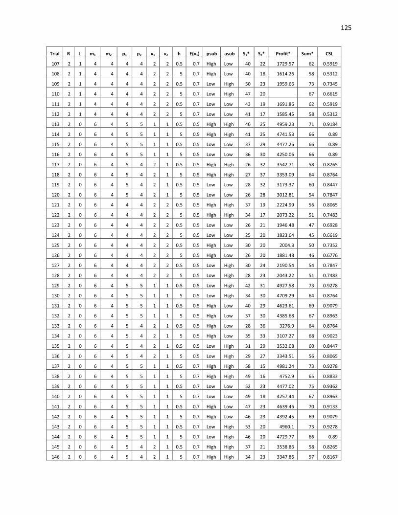
125

Trial R L m1 m2 p1 p2 v1 v2 h E(κ1) psub asub S1* S2* Profit* Sum* CSL

107 2 1 4 4 4 4 2 2 0.5 0.7 High Low 40 22 1729.57 62 0.5919

108 2 1 4 4 4 4 2 2 5 0.7 High Low 40 18 1614.26 58 0.5312

109 2 1 4 4 4 4 2 2 0.5 0.7 Low High 50 23 1959.66 73 0.7345

110 2 1 4 4 4 4 2 2 5 0.7 Low High 47 20

67 0.6615

111 2 1 4 4 4 4 2 2 0.5 0.7 Low Low 43 19 1691.86 62 0.5919

112 2 1 4 4 4 4 2 2 5 0.7 Low Low 41 17 1585.45 58 0.5312

113 2 0 6 4 5 5 1 1 0.5 0.5 High High 46 25 4959.23 71 0.9184

114 2 0 6 4 5 5 1 1 5 0.5 High High 41 25 4741.53 66 0.89

115 2 0 6 4 5 5 1 1 0.5 0.5 Low Low 37 29 4477.26 66 0.89

116 2 0 6 4 5 5 1 1 5 0.5 Low Low 36 30 4250.06 66 0.89

117 2 0 6 4 5 4 2 1 0.5 0.5 High High 26 32 3542.71 58 0.8265

118 2 0 6 4 5 4 2 1 5 0.5 High High 27 37 3353.09 64 0.8764

119 2 0 6 4 5 4 2 1 0.5 0.5 Low Low 28 32 3173.37 60 0.8447

120 2 0 6 4 5 4 2 1 5 0.5 Low Low 26 28 3012.81 54 0.7847

121 2 0 6 4 4 4 2 2 0.5 0.5 High High 37 19 2224.99 56 0.8065

122 2 0 6 4 4 4 2 2 5 0.5 High High 34 17 2073.22 51 0.7483

123 2 0 6 4 4 4 2 2 0.5 0.5 Low Low 26 21 1946.48 47 0.6928

124 2 0 6 4 4 4 2 2 5 0.5 Low Low 25 20 1823.64 45 0.6619

125 2 0 6 4 4 4 2 2 0.5 0.5 High Low 30 20 2004.3 50 0.7352

126 2 0 6 4 4 4 2 2 5 0.5 High Low 26 20 1881.48 46 0.6776

127 2 0 6 4 4 4 2 2 0.5 0.5 Low High 30 24 2190.54 54 0.7847

128 2 0 6 4 4 4 2 2 5 0.5 Low High 28 23 2043.22 51 0.7483

129 2 0 6 4 5 5 1 1 0.5 0.5 Low High 42 31 4927.58 73 0.9278

130 2 0 6 4 5 5 1 1 5 0.5 Low High 34 30 4709.29 64 0.8764

131 2 0 6 4 5 5 1 1 0.5 0.5 High Low 40 29 4623.61 69 0.9079

132 2 0 6 4 5 5 1 1 5 0.5 High Low 37 30 4385.68 67 0.8963

133 2 0 6 4 5 4 2 1 0.5 0.5 High Low 28 36 3276.9 64 0.8764

134 2 0 6 4 5 4 2 1 5 0.5 High Low 35 33 3107.27 68 0.9023

135 2 0 6 4 5 4 2 1 0.5 0.5 Low High 31 29 3532.08 60 0.8447

136 2 0 6 4 5 4 2 1 5 0.5 Low High 29 27 3343.51 56 0.8065

137 2 0 6 4 5 5 1 1 0.5 0.7 High High 58 15 4981.24 73 0.9278

138 2 0 6 4 5 5 1 1 5 0.7 High High 49 16 4752.9 65 0.8833

139 2 0 6 4 5 5 1 1 0.5 0.7 Low Low 52 23 4477.02 75 0.9362

140 2 0 6 4 5 5 1 1 5 0.7 Low Low 49 18 4257.44 67 0.8963

141 2 0 6 4 5 5 1 1 0.5 0.7 High Low 47 23 4639.46 70 0.9133

142 2 0 6 4 5 5 1 1 5 0.7 High Low 46 23 4392.45 69 0.9079

143 2 0 6 4 5 5 1 1 0.5 0.7 Low High 53 20 4960.1 73 0.9278

144 2 0 6 4 5 5 1 1 5 0.7 Low High 46 20 4729.77 66 0.89

145 2 0 6 4 5 4 2 1 0.5 0.7 High High 37 21 3538.86 58 0.8265

146 2 0 6 4 5 4 2 1 5 0.7 High High 34 23 3347.86 57 0.8167

126

Trial R L m1 m2 p1 p2 v1 v2 h E(κ1) psub asub S1* S2* Profit* Sum* CSL

147 2 0 6 4 5 4 2 1 0.5 0.7 High Low 35 21 3260.89 56 0.8065

148 2 0 6 4 5 4 2 1 5 0.7 High Low 32 20 3089.27 52 0.7609

149 2 0 6 4 5 4 2 1 0.5 0.7 Low High 43 20 3520.24 63 0.869

150 2 0 6 4 5 4 2 1 5 0.7 Low High 41 21 3335.51 62 0.8613

151 2 0 6 4 5 4 2 1 0.5 0.7 Low Low 38 22 3155.39 60 0.8447

152 2 0 6 4 5 4 2 1 5 0.7 Low Low 40 20 2972.19 60 0.8447

153 2 0 6 4 4 5 1 2 0.5 0.7 High Low 49 13 3295.11 62 0.8613

154 2 0 6 4 4 5 1 2 5 0.7 High Low 44 15 3096.18 59 0.8358

155 2 0 6 4 4 5 1 2 0.5 0.7 Low High 48 15 3579.96 63 0.869

156 2 0 6 4 4 5 1 2 5 0.7 Low High 43 15 3374.33 58 0.8265

157 2 0 6 4 4 5 1 2 0.5 0.7 Low Low 44 13 3208.37 57 0.8167

158 2 0 6 4 4 5 1 2 5 0.7 Low Low 40 14 3023.41 54 0.7847

159 2 0 6 4 4 5 1 2 0.5 0.7 High High 55 11 3636.18 66 0.89

160 2 0 6 4 4 5 1 2 5 0.7 High High 48 11 3429.92 59 0.8358

161 2 0 6 4 4 4 2 2 0.5 0.7 High High 46 11 2236.58 57 0.8167

162 2 0 6 4 4 4 2 2 5 0.7 High High 43 9 2082.26 52 0.7609

163 2 0 6 4 4 4 2 2 0.5 0.7 High Low 37 14 2018.82 51 0.7483

164 2 0 6 4 4 4 2 2 5 0.7 High Low 29 16 1879.57 45 0.6619

165 2 0 6 4 4 4 2 2 0.5 0.7 Low Low 35 15 1957.13 50 0.7352

166 2 0 6 4 4 4 2 2 5 0.7 Low Low 31 12 1831.64 43 0.629

167 2 0 6 4 4 4 2 2 0.5 0.7 Low High 42 15 2208.88 57 0.8167

168 2 0 6 4 4 4 2 2 5 0.7 Low High 40 13 2054.24 53 0.773

169 2 1 6 4 5 5 1 1 0.5 0.5 High High 57 44 4822.84 101 0.9313

170 2 1 6 4 5 5 1 1 5 0.5 High High 57 44 4583.75 101 0.9313

171 2 1 6 4 5 5 1 1 0.5 0.5 Low Low 56 50 4292.41 106 0.9476

172 2 1 6 4 5 5 1 1 5 0.5 Low Low 50 49 4068.21 99 0.9235

173 2 1 6 4 5 4 2 1 0.5 0.5 High High 47 49 3427.33 96 0.9105

174 2 1 6 4 5 4 2 1 5 0.5 High High 42 47 3238.96 89 0.8725

175 2 1 6 4 5 4 2 1 0.5 0.5 Low Low 40 44 3028.76 84 0.8377

176 2 1 6 4 5 4 2 1 5 0.5 Low Low 40 44 2844.82 84 0.8377

177 2 1 6 4 4 4 2 2 0.5 0.5 High High 49 27 2134.43 76 0.7665

178 2 1 6 4 4 4 2 2 5 0.5 High High 42 26 1984.39 68 0.6745

179 2 1 6 4 4 4 2 2 0.5 0.5 Low Low 38 30 1822.67 68 0.6745

180 2 1 6 4 4 4 2 2 5 0.5 Low Low 33 28 1703.25 61 0.5771

181 2 1 6 4 4 4 2 2 0.5 0.5 High Low 42 26 1902.27 68 0.6745

182 2 1 6 4 4 4 2 2 5 0.5 High Low 41 24 1773.9 65 0.6346

183 2 1 6 4 4 4 2 2 0.5 0.5 Low High 41 32 2082.42 73 0.7345

184 2 1 6 4 4 4 2 2 5 0.5 Low High 39 30 1934.71 69 0.6871

185 2 1 6 4 5 5 1 1 0.5 0.5 Low High 64 53 4743 117 0.972

186 2 1 6 4 5 5 1 1 5 0.5 Low High 52 47 4515.49 99 0.9235

127

Trial R L m1 m2 p1 p2 v1 v2 h E(κ1) psub asub S1* S2* Profit* Sum* CSL

187 2 1 6 4 5 5 1 1 0.5 0.5 High Low 63 52 4467.07 115 0.9685

188 2 1 6 4 5 5 1 1 5 0.5 High Low 53 47 4234.66 100 0.9275

189 2 1 6 4 5 4 2 1 0.5 0.5 High Low 38 55 3155.58 93 0.8956

190 2 1 6 4 5 4 2 1 5 0.5 High Low 36 48 2968.2 84 0.8377

191 2 1 6 4 5 4 2 1 0.5 0.5 Low High 43 51 3385.83 94 0.9008

192 2 1 6 4 5 4 2 1 5 0.5 Low High 43 42 3192.84 85 0.8452

193 2 1 6 4 5 5 1 1 0.5 0.7 High High 69 30 4860.15 99 0.9235

194 2 1 6 4 5 5 1 1 5 0.7 High High 74 24 4617.89 98 0.9194

195 2 1 6 4 5 5 1 1 0.5 0.7 Low Low 70 31 4329.41 101 0.9313

196 2 1 6 4 5 5 1 1 5 0.7 Low Low 70 27 4093.79 97 0.915

197 2 1 6 4 5 5 1 1 0.5 0.7 High Low 70 35 4501.01 105 0.9447

198 2 1 6 4 5 5 1 1 5 0.7 High Low 64 34 4255.58 98 0.9194

199 2 1 6 4 5 5 1 1 0.5 0.7 Low High 73 30 4805.05 103 0.9383

200 2 1 6 4 5 5 1 1 5 0.7 Low High 70 30 4549.25 100 0.9275

201 2 1 6 4 5 4 2 1 0.5 0.7 High High 60 32 3431.25 92 0.8902

202 2 1 6 4 5 4 2 1 5 0.7 High High 55 31 3246.52 86 0.8524

203 2 1 6 4 5 4 2 1 0.5 0.7 High Low 50 42 3162.05 92 0.8902

204 2 1 6 4 5 4 2 1 5 0.7 High Low 48 31 2976.75 79 0.7956

205 2 1 6 4 5 4 2 1 0.5 0.7 Low High 55 30 3382.34 85 0.8452

206 2 1 6 4 5 4 2 1 5 0.7 Low High 57 29 3197.29 86 0.8524

207 2 1 6 4 5 4 2 1 0.5 0.7 Low Low 54 28 3017.25 82 0.8217

208 2 1 6 4 5 4 2 1 5 0.7 Low Low 48 26 2849.04 74 0.7455

209 2 1 6 4 4 5 1 2 0.5 0.7 High Low 74 21 3185.04 95 0.9058

210 2 1 6 4 4 5 1 2 5 0.7 High Low 61 18 2983.72 79 0.7956

211 2 1 6 4 4 5 1 2 0.5 0.7 Low High 73 25 3463.23 98 0.9194

212 2 1 6 4 4 5 1 2 5 0.7 Low High 67 23 3253.89 90 0.8986

213 2 1 6 4 4 5 1 2 0.5 0.7 Low Low 64 21 3001.88 85 0.8452

214 2 1 6 4 4 5 1 2 5 0.7 Low Low 57 19 2818.46 76 0.7665

215 2 1 6 4 4 5 1 2 0.5 0.7 High High 82 17 3523.71 99 0.9235

216 2 1 6 4 4 5 1 2 5 0.7 High High 78 15 3303.65 93 0.8956

217 2 1 6 4 4 4 2 2 0.5 0.7 High High 62 15 2147.52 77 0.7765

218 2 1 6 4 4 4 2 2 5 0.7 High High 55 14 1997.52 69 0.6871

219 2 1 6 4 4 4 2 2 0.5 0.7 High Low 50 19 1920.33 69 0.6871

220 2 1 6 4 4 4 2 2 5 0.7 High Low 49 18 1789.24 67 0.6615

221 2 1 6 4 4 4 2 2 0.5 0.7 Low Low 48 19 1848.2 67 0.6615

222 2 1 6 4 4 4 2 2 5 0.7 Low Low 48 16 1721.08 64 0.6206

223 2 1 6 4 4 4 2 2 0.5 0.7 Low High 54 20 2101.09 74 0.7455

224 2 1 6 4 4 4 2 2 5 0.7 Low High 52 20 1953.19 72 0.7232

225 2 0 4 6 5 5 1 1 0.5 0.7 High High 36 34 4947.21 70 0.9133

226 2 0 4 6 5 5 1 1 5 0.7 High High 34 31 4720.44 65 0.8833

128

Trial R L m1 m2 p1 p2 v1 v2 h E(κ1) psub asub S1* S2* Profit* Sum* CSL

227 2 0 4 6 5 5 1 1 0.5 0.7 Low Low 46 24 4447.79 70 0.9133

228 2 0 4 6 5 5 1 1 5 0.7 Low Low 40 21 4238.62 61 0.8532

229 2 0 4 6 5 5 1 1 0.5 0.7 High Low 47 30 4593.88 77 0.9437

230 2 0 4 6 5 5 1 1 5 0.7 High Low 33 31 4368.54 64 0.8764

231 2 0 4 6 5 5 1 1 0.5 0.7 Low High 44 25 4902.45 69 0.9079

232 2 0 4 6 5 5 1 1 5 0.7 Low High 41 23 4682.29 64 0.8764

233 2 0 4 6 5 4 2 1 0.5 0.7 High High 26 42 3564.5 68 0.9023

234 2 0 4 6 5 4 2 1 5 0.7 High High 31 31 3365 62 0.8613

235 2 0 4 6 5 4 2 1 0.5 0.7 High Low 24 36 3257.38 60 0.8447

236 2 0 4 6 5 4 2 1 5 0.7 High Low 25 30 3065.06 55 0.7958

237 2 0 4 6 5 4 2 1 0.5 0.7 Low High 35 23 3465.36 58 0.8265

238 2 0 4 6 5 4 2 1 5 0.7 Low High 33 23 3276.54 56 0.8065

239 2 0 4 6 5 4 2 1 0.5 0.7 Low Low 25 29 3109.48 54 0.7847

240 2 0 4 6 5 4 2 1 5 0.7 Low Low 33 21 2946.17 54 0.7847

241 2 0 4 6 4 5 1 2 0.5 0.7 High Low 48 18 3272.5 66 0.89

242 2 0 4 6 4 5 1 2 5 0.7 High Low 37 19 3100.43 56 0.8065

243 2 0 4 6 4 5 1 2 0.5 0.7 Low High 45 19 3526.16 64 0.8764

244 2 0 4 6 4 5 1 2 5 0.7 Low High 37 19 3337.08 56 0.8065

245 2 0 4 6 4 5 1 2 0.5 0.7 Low Low 39 17 3177.32 56 0.8065

246 2 0 4 6 4 5 1 2 5 0.7 Low Low 39 17 3022.94 56 0.8065

247 2 0 4 6 4 5 1 2 0.5 0.7 High High 45 18 3543.81 63 0.869

248 2 0 4 6 4 5 1 2 5 0.7 High High 40 21 3356.7 61 0.8532

249 2 0 4 6 4 4 2 2 0.5 0.7 High High 27 28 2206.68 55 0.7958

250 2 0 4 6 4 4 2 2 5 0.7 High High 27 24 2060.13 51 0.7483

251 2 0 4 6 4 4 2 2 0.5 0.7 High Low 28 20 1994.51 48 0.7074

252 2 0 4 6 4 4 2 2 5 0.7 High Low 27 20 1868.85 47 0.6928

253 2 0 4 6 4 4 2 2 0.5 0.7 Low Low 29 17 1926.75 46 0.6776

254 2 0 4 6 4 4 2 2 5 0.7 Low Low 27 16 1807.06 43 0.629

255 2 0 4 6 4 4 2 2 0.5 0.7 Low High 35 18 2158.21 53 0.773

256 2 0 4 6 4 4 2 2 5 0.7 Low High 32 17 2018.85 49 0.7216

257 2 1 4 6 5 5 1 1 0.5 0.7 High High 60 51 4808.29 111 0.9604

258 2 1 4 6 5 5 1 1 5 0.7 High High 58 47 4571.95 105 0.9447

259 2 1 4 6 5 5 1 1 0.5 0.7 Low Low 66 37 4527.12 103 0.9383

260 2 1 4 6 5 5 1 1 5 0.7 Low Low 60 38 4019.88 98 0.9194

261 2 1 4 6 5 5 1 1 0.5 0.7 High Low 61 51 4443.73 112 0.9626

262 2 1 4 6 5 5 1 1 5 0.7 High Low 54 49 4206.31 103 0.9393

263 2 1 4 6 5 5 1 1 0.5 0.7 Low High 67 39 4709.67 106 0.9476

264 2 1 4 6 5 5 1 1 5 0.7 Low High 63 38 4479.75 101 0.9313

265 2 1 4 6 5 4 2 1 0.5 0.7 High High 40 55 3450.32 95 0.9058

266 2 1 4 6 5 4 2 1 5 0.7 High High 40 46 3243 86 0.8524

129

Trial R L m1 m2 p1 p2 v1 v2 h E(κ1) psub asub S1* S2* Profit* Sum* CSL

267 2 1 4 6 5 4 2 1 0.5 0.7 High Low 41 55 3085.12 96 0.9105

268 2 1 4 6 5 4 2 1 5 0.7 High Low 40 43 2886.4 83 0.8298

269 2 1 4 6 5 4 2 1 0.5 0.7 Low High 51 37 3301.54 88 0.866

270 2 1 4 6 5 4 2 1 5 0.7 Low High 51 31 3114.2 82 0.8217

271 2 1 4 6 5 4 2 1 0.5 0.7 Low Low 42 38 2922.44 80 0.8046

272 2 1 4 6 5 4 2 1 5 0.7 Low Low 46 32 2757.87 78 0.7862

273 2 1 4 6 4 5 1 2 0.5 0.7 High Low 63 23 3095.76 86 0.8524

274 2 1 4 6 4 5 1 2 5 0.7 High Low 56 28 2911.92 84 0.8377

275 2 1 4 6 4 5 1 2 0.5 0.7 Low High 65 30 3374.89 95 0.9058

276 2 1 4 6 4 5 1 2 5 0.7 Low High 60 25 3181.21 85 0.8452

277 2 1 4 6 4 5 1 2 0.5 0.7 Low Low 60 26 3021.74 86 0.8524

278 2 1 4 6 4 5 1 2 5 0.7 Low Low 57 22 2839.33 79 0.7956

279 2 1 4 6 4 5 1 2 0.5 0.7 High High 60 32 3424.18 92 0.8902

280 2 1 4 6 4 5 1 2 5 0.7 High High 57 30 3231.56 87 0.8594

281 2 1 4 6 4 4 2 2 0.5 0.7 High High 40 39 2114.61 79 0.7956

282 2 1 4 6 4 4 2 2 5 0.7 High High 40 33 1967.8 79 0.7956

283 2 1 4 6 4 4 2 2 0.5 0.7 High Low 40 32 1876.02 72 0.7231

284 2 1 4 6 4 4 2 2 5 0.7 High Low 40 29 1744.41 69 0.6871

285 2 1 4 6 4 4 2 2 0.5 0.7 Low Low 42 22 1780.97 64 0.6206

286 2 1 4 6 4 4 2 2 5 0.7 Low Low 49 21 1661.27 70 0.6995

287 2 1 4 6 4 4 2 2 0.5 0.7 Low High 47 28 2046.78 75 0.7562

288 2 1 4 6 4 4 2 2 5 0.7 Low High 44 26 1906.21 70 0.6995

289 2 0 6 6 5 5 1 1 0.5 0.5 High High 35 35 5003.93 70 0.9133

290 2 0 6 6 5 5 1 1 5 0.5 High High 32 32 4768.64 64 0.8763

291 2 0 6 6 5 5 1 1 0.5 0.5 Low Low 33 33 4515.19 66 0.89

292 2 0 6 6 5 5 1 1 5 0.5 Low Low 35 35 4285.16 70 0.9133

293 2 0 6 6 5 4 2 1 0.5 0.5 High High 21 46 3649.02 67 0.8963

294 2 0 6 6 5 4 2 1 5 0.5 High High 19 42 3441.86 61 0.8532

295 2 0 6 6 5 4 2 1 0.5 0.5 Low Low 26 40 3212.05 66 0.89

296 2 0 6 6 5 4 2 1 5 0.5 Low Low 25 33 3047.67 58 0.8265

297 2 0 6 6 4 4 2 2 0.5 0.5 High High 28 28 2268.27 56 0.8065

298 2 0 6 6 4 4 2 2 5 0.5 High High 27 27 2110.26 54 0.7847

299 2 0 6 6 4 4 2 2 0.5 0.5 Low Low 24 24 1999.2 48 0.7074

300 2 0 6 6 4 4 2 2 5 0.5 Low Low 24 24 1870.78 48 0.7074

301 2 0 6 6 4 4 2 2 0.5 0.5 High Low 24 24 2038.75 48 0.7074

302 2 0 6 6 4 4 2 2 5 0.5 High Low 24 24 1908.82 48 0.7074

303 2 0 6 6 4 4 2 2 0.5 0.5 Low High 29 29 2255.97 58 0.8265

304 2 0 6 6 4 4 2 2 5 0.5 Low High 27 27 2101.54 54 0.7847

305 2 0 6 6 5 5 1 1 0.5 0.5 Low High 37 37 5000.53 74 0.9321

306 2 0 6 6 5 5 1 1 5 0.5 Low High 33 33 4762.37 66 0.89

130

Trial R L m1 m2 p1 p2 v1 v2 h E(κ1) psub asub S1* S2* Profit* Sum* CSL

307 2 0 6 6 5 5 1 1 0.5 0.5 High Low 29 29 4369.81 58 0.8265

308 2 0 6 6 5 5 1 1 5 0.5 High Low 31 31 4581.48 62 0.8613

309 2 0 6 6 5 4 2 1 0.5 0.5 High Low 23 44 3305.33 67 0.8963

310 2 0 6 6 5 4 2 1 5 0.5 High Low 20 36 3117.55 56 0.8065

311 2 0 6 6 5 4 2 1 0.5 0.5 Low High 29 35 3607.97 64 0.8763

312 2 0 6 6 5 4 2 1 5 0.5 Low High 26 36 3387.14 62 0.8613

313 2 0 6 6 5 5 1 1 0.5 0.7 High High 45 27 5012.62 72 0.9232

314 2 0 6 6 5 5 1 1 5 0.7 High High 48 17 4771.11 65 0.8833

315 2 0 6 6 5 5 1 1 0.5 0.7 Low Low 48 22 4509.17 70 0.9133

316 2 0 6 6 5 5 1 1 5 0.7 Low Low 50 21 4279.89 71 0.9133

317 2 0 6 6 5 5 1 1 0.5 0.7 High Low 52 23 4584.79 75 0.9362

318 2 0 6 6 5 5 1 1 5 0.7 High Low 46 23 4366.99 69 0.9069

319 2 0 6 6 5 5 1 1 0.5 0.7 Low High 49 24 4997.59 73 0.9278

320 2 0 6 6 5 5 1 1 5 0.7 Low High 47 20 4766.77 67 0.8963

321 2 0 6 6 5 4 2 1 0.5 0.7 High High 33 32 3636.52 65 0.8833

322 2 0 6 6 5 4 2 1 5 0.7 High High 28 31 3431.77 59 0.8358

323 2 0 6 6 5 4 2 1 0.5 0.7 High Low 34 27 3287.51 61 0.8532

324 2 0 6 6 5 4 2 1 5 0.7 High Low 30 24 3107.59 54 0.7847

325 2 0 6 6 5 4 2 1 0.5 0.7 Low High 42 25 3565.24 67 0.8963

326 2 0 6 6 5 4 2 1 5 0.7 Low High 42 24 3363.78 66 0.89

327 2 0 6 6 5 4 2 1 0.5 0.7 Low Low 33 21 3197.3 54 0.7847

328 2 0 6 6 5 4 2 1 5 0.7 Low Low 35 21 3021.88 56 0.8065

329 2 0 6 6 4 5 1 2 0.5 0.7 High Low 54 10 3323.04 64 0.8763

330 2 0 6 6 4 5 1 2 5 0.7 High Low 44 14 3137.9 58 0.8265

331 2 0 6 6 4 5 1 2 0.5 0.7 Low High 49 19 3623.16 68 0.9023

332 2 0 6 6 4 5 1 2 5 0.7 Low High 45 17 3416.49 62 0.8613

333 2 0 6 6 4 5 1 2 0.5 0.7 Low Low 49 20 3223.56 69 0.9069

334 2 0 6 6 4 5 1 2 5 0.7 Low Low 42 16 3070.33 58 0.8265

335 2 0 6 6 4 5 1 2 0.5 0.7 High High 56 12 3666.67 68 0.9023

336 2 0 6 6 4 5 1 2 5 0.7 High High 47 13 3453.49 60 0.8447

337 2 0 6 6 4 4 2 2 0.5 0.7 High High 39 18 2270.02 57 0.8167

338 2 0 6 6 4 4 2 2 5 0.7 High High 34 19 2114.48 53 0.773

339 2 0 6 6 4 4 2 2 0.5 0.7 High Low 35 18 2039.6 53 0.773

340 2 0 6 6 4 4 2 2 5 0.7 High Low 33 15 1912.94 48 0.7047

341 2 0 6 6 4 4 2 2 0.5 0.7 Low Low 34 17 1994.47 51 0.7483

342 2 0 6 6 4 4 2 2 5 0.7 Low Low 33 15 1868.92 48 0.7047

343 2 0 6 6 4 4 2 2 0.5 0.7 Low High 39 19 2253.85 58 0.8265

344 2 0 6 6 4 4 2 2 5 0.7 Low High 36 18 ------------ 54 0.7847

345 2 1 6 6 5 5 1 1 0.5 0.5 High High 52 52 4871.12 104 0.9415

346 2 1 6 6 5 5 1 1 5 0.5 High High 49 49 4634.92 98 0.9194

131

Trial R L m1 m2 p1 p2 v1 v2 h E(κ1) psub asub S1* S2* Profit* Sum* CSL

347 2 1 6 6 5 5 1 1 0.5 0.5 Low Low 51 51 4369.14 102 0.9349

348 2 1 6 6 5 5 1 1 5 0.5 Low Low 45 45 4135.51 90 0.8786

349 2 1 6 6 5 4 2 1 0.5 0.5 High High 31 67 3543.37 98 0.9194

350 2 1 6 6 5 4 2 1 5 0.5 High High 31 55 ------------ 86 0.8524

351 2 1 6 6 5 4 2 1 0.5 0.5 Low Low 39 42 3092.23 81 0.8133

352 2 1 6 6 5 4 2 1 5 0.5 Low Low 37 41 2909.5 78 0.7862

353 2 1 6 6 4 4 2 2 0.5 0.5 High High 38 38 2187.31 76 0.7665

354 2 1 6 6 4 4 2 2 5 0.5 High High 36 36 2027.83 72 0.7232

355 2 1 6 6 4 4 2 2 0.5 0.5 Low Low 33 33 1901 66 0.6482

356 2 1 6 6 4 4 2 2 5 0.5 Low Low 31 31 1775.63 62 0.5919

357 2 1 6 6 4 4 2 2 0.5 0.5 High Low 35 35 1947.9 70 0.6995

358 2 1 6 6 4 4 2 2 5 0.5 High Low 31 31 1815.62 62 0.5919

359 2 1 6 6 4 4 2 2 0.5 0.5 Low High 38 38 2169.35 76 0.7665

360 2 1 6 6 4 4 2 2 5 0.5 Low High 35 35 2012 70 0.6995

361 2 1 6 6 5 5 1 1 0.5 0.5 Low High 52 52 4869.18 104 0.9416

362 2 1 6 6 5 5 1 1 5 0.5 Low High 47 47 4619.62 94 0.9008

363 2 1 6 6 5 5 1 1 0.5 0.5 High Low 44 44 4213.5 88 0.866

364 2 1 6 6 5 5 1 1 5 0.5 High Low 48 48 4454.38 96 0.9105

365 2 1 6 6 5 4 2 1 0.5 0.5 High Low 21 63 3296.45 84 0.8377

366 2 1 6 6 5 4 2 1 5 0.5 High Low 25 53 3074.42 78 0.7862

367 2 1 6 6 5 4 2 1 0.5 0.5 Low High 38 58 3515.31 96 0.9105

368 2 1 6 6 5 4 2 1 5 0.5 Low High 39 50 3307.68 89 0.8725

369 2 1 6 6 5 5 1 1 0.5 0.7 High High 72 32 4886.99 104 0.9416

370 2 1 6 6 5 5 1 1 5 0.7 High High 66 33 4645.44 99 0.9235

371 2 1 6 6 5 5 1 1 0.5 0.7 Low Low 68 32 4361.38 100 0.9275

372 2 1 6 6 5 5 1 1 5 0.7 Low Low 59 29 4134.98 88 0.866

373 2 1 6 6 5 5 1 1 0.5 0.7 High Low 59 40 4464.05 99 0.9235

374 2 1 6 6 5 5 1 1 5 0.7 High Low 55 34 4221.03 89 0.8725

375 2 1 6 6 5 5 1 1 0.5 0.7 Low High 72 28 4863.85 100 0.9275

376 2 1 6 6 5 5 1 1 5 0.7 Low High 67 28 4614.6 95 0.9058

377 2 1 6 6 5 4 2 1 0.5 0.7 High High 47 49 3525.25 96 0.9105

378 2 1 6 6 5 4 2 1 5 0.7 High High 45 44 3314.78 89 0.8725

379 2 1 6 6 5 4 2 1 0.5 0.7 High Low 41 47 3175.9 88 0.866

380 2 1 6 6 5 4 2 1 5 0.7 High Low 39 41 2981.73 80 0.8046

381 2 1 6 6 5 4 2 1 0.5 0.7 Low High 57 36 3457.75 93 0.8956

382 2 1 6 6 5 4 2 1 5 0.7 Low High 55 29 3259.52 84 0.8377

383 2 1 6 6 5 4 2 1 0.5 0.7 Low Low 50 32 3062.39 82 0.8217

384 2 1 6 6 5 4 2 1 5 0.7 Low Low 49 31 2880.24 80 0.8046

385 2 1 6 6 4 5 1 2 0.5 0.7 High Low 77 18 3216.14 95 0.9058

386 2 1 6 6 4 5 1 2 5 0.7 High Low 64 17 3002.94 81 0.8133

132

Trial R L m1 m2 p1 p2 v1 v2 h E(κ1) psub asub S1* S2* Profit* Sum* CSL

387 2 1 6 6 4 5 1 2 0.5 0.7 Low High 71 25 3516.54 96 0.9105

388 2 1 6 6 4 5 1 2 5 0.7 Low High 65 23 3302.94 88 0.866

389 2 1 6 6 4 5 1 2 0.5 0.7 Low Low 65 20 3129.16 85 0.8452

390 2 1 6 6 4 5 1 2 5 0.7 Low Low 61 20 2930.3 81 0.8133

391 2 1 6 6 4 5 1 2 0.5 0.7 High High 77 20 3553.2 97 0.915

392 2 1 6 6 4 5 1 2 5 0.7 High High 71 18 3337.64 89 0.8725

393 2 1 6 6 4 4 2 2 0.5 0.7 High High 50 31 2185.76 81 0.8133

394 2 1 6 6 4 4 2 2 5 0.7 High High 47 26 2030.76 73 0.7435

395 2 1 6 6 4 4 2 2 0.5 0.7 High Low 46 22 1951.76 68 0.6745

396 2 1 6 6 4 4 2 2 5 0.7 High Low 42 23 1817.23 65 0.6346

397 2 1 6 6 4 4 2 2 0.5 0.7 Low Low 50 20 1900.36 70 0.6995

398 2 1 6 6 4 4 2 2 5 0.7 Low Low 43 19 1771.99 62 0.5919

399 2 1 6 6 4 4 2 2 0.5 0.7 Low High 54 26 2169.85 80 0.8056

400 2 1 6 6 4 4 2 2 5 0.7 Low High 51 23 2012.92 74 0.7455

401 3 0 4 4 5 5 1 1 0.5 0.5 High High 47 47 4151.76 94 0.9008

402 3 0 4 4 5 5 1 1 5 0.5 High High 43 43 3937.71 86 0.8524

403 3 0 4 4 5 5 1 1 0.5 0.5 Low Low 40 40 3313.2 80 0.8046

404 3 0 4 4 5 5 1 1 5 0.5 Low Low 36 36 3147.4 72 0.7232

405 3 0 4 4 5 4 2 1 0.5 0.5 High High 28 50 2960.36 78 0.7862

406 3 0 4 4 5 4 2 1 5 0.5 High High 24 51 2788.5 75 0.7562

407 3 0 4 4 5 4 2 1 0.5 0.5 Low Low 27 38 2324.17 65 0.6346

408 3 0 4 4 5 4 2 1 5 0.5 Low Low 27 24 2193.89 51 0.4173

409 3 0 4 4 4 4 2 2 0.5 0.5 High High 31 31 1761.17 62 0.5919

410 3 0 4 4 4 4 2 2 5 0.5 High High 30 30 1638.02 60 0.562

411 3 0 4 4 4 4 2 2 0.5 0.5 Low Low 25 25 1388.2 50 0.4006

412 3 0 4 4 4 4 2 2 5 0.5 Low Low 24 24 1299.31 48 0.3672

413 3 0 4 4 4 4 2 2 0.5 0.5 High Low 26 26 1394.79 52 0.44

414 3 0 4 4 4 4 2 2 5 0.5 High Low 24 24 1304.17 48 0.3672

415 3 0 4 4 4 4 2 2 0.5 0.5 Low High 31 31 1741.53 62 0.5919

416 3 0 4 4 4 4 2 2 5 0.5 Low High 30 30 1614.95 60 0.562

417 3 0 4 4 5 5 1 1 0.5 0.5 Low High 45 45 4114.96 90 0.8786

418 3 0 4 4 5 5 1 1 5 0.5 Low High 44 44 3900.82 88 0.866

419 3 0 4 4 5 5 1 1 0.5 0.5 High Low 41 41 3330.31 82 0.8217

420 3 0 4 4 5 5 1 1 5 0.5 High Low 36 36 3170.6 72 0.7232

421 3 0 4 4 5 4 2 1 0.5 0.5 High Low 25 42 2353.53 67 0.6615

422 3 0 4 4 5 4 2 1 5 0.5 High Low 24 38 2224.71 62 0.5919

423 3 0 4 4 5 4 2 1 0.5 0.5 Low High 34 45 2882.4 79 0.7956

424 3 0 4 4 5 4 2 1 5 0.5 Low High 33 42 2711.05 75 0.7562

425 3 0 4 4 5 5 1 1 0.5 0.7 High High 60 34 4154.72 94 0.9008

426 3 0 4 4 5 5 1 1 5 0.7 High High 61 24 3940.65 85 0.8452

133

Trial R L m1 m2 p1 p2 v1 v2 h E(κ1) psub asub S1* S2* Profit* Sum* CSL

427 3 0 4 4 5 5 1 1 0.5 0.7 Low Low 53 24 3312.83 77 0.7765

428 3 0 4 4 5 5 1 1 5 0.7 Low Low 49 28 3142.91 77 0.7765

429 3 0 4 4 5 5 1 1 0.5 0.7 High Low 57 24 3334.72 81 0.8133

430 3 0 4 4 5 5 1 1 5 0.7 High Low 52 23 3162.95 75 0.7562

431 3 0 4 4 5 5 1 1 0.5 0.7 Low High 67 31 4102.33 98 0.9194

432 3 0 4 4 5 5 1 1 5 0.7 Low High 61 28 3894.21 89 0.8725

433 3 0 4 4 5 4 2 1 0.5 0.7 High High 36 45 2949.11 81 0.8133

434 3 0 4 4 5 4 2 1 5 0.7 High High 34 43 2773.12 77 0.7765

435 3 0 4 4 5 4 2 1 0.5 0.7 High Low 31 33 2333.92 64 0.6206

436 3 0 4 4 5 4 2 1 5 0.7 High Low 31 27 2203.8 58 0.5311

437 3 0 4 4 5 4 2 1 0.5 0.7 Low High 48 29 2840.32 77 0.7765

438 3 0 4 4 5 4 2 1 5 0.7 Low High 45 27 2673.59 72 0.7232

439 3 0 4 4 5 4 2 1 0.5 0.7 Low Low 37 35 2293.55 72 0.7232

440 3 0 4 4 5 4 2 1 5 0.7 Low Low 34 24 2169.12 58 0.5312

441 3 0 4 4 4 5 1 2 0.5 0.7 High Low 55 15 2378.56 70 0.6995

442 3 0 4 4 4 5 1 2 5 0.7 High Low 50 13 2237.79 63 0.6064

443 3 0 4 4 4 5 1 2 0.5 0.7 Low High 61 20 2921.42 81 0.8133

444 3 0 4 4 4 5 1 2 5 0.7 Low High 60 19 2741.53 79 0.7956

445 3 0 4 4 4 5 1 2 0.5 0.7 Low Low 50 16 2348.11 66 0.6482

446 3 0 4 4 4 5 1 2 5 0.7 Low Low 50 15 2212.2 65 0.6346

447 3 0 4 4 4 5 1 2 0.5 0.7 High High 69 15 2988.2 84 0.8377

448 3 0 4 4 4 5 1 2 5 0.7 High High 63 14 2804.57 77 0.7765

449 3 0 4 4 4 4 2 2 0.5 0.7 High High 42 19 1762.56 61 0.5771

450 3 0 4 4 4 4 2 2 5 0.7 High High 40 20 1641.28 60 0.562

451 3 0 4 4 4 4 2 2 0.5 0.7 High Low 33 16 1396.08 49 0.3839

452 3 0 4 4 4 4 2 2 5 0.7 High Low 30 18 1308.62 48 0.3672

453 3 0 4 4 4 4 2 2 0.5 0.7 Low Low 32 17 1390.72 49 0.3839

454 3 0 4 4 4 4 2 2 5 0.7 Low Low 32 17 1302.37 49 0.3839

455 3 0 4 4 4 4 2 2 0.5 0.7 Low High 44 19 1735.71 63 0.6064

456 3 0 4 4 4 4 2 2 5 0.7 Low High 42 18 1611.33 60 0.562

457 3 0 6 4 5 5 1 1 0.5 0.5 High High 69 24 4810.17 93 0.8956

458 3 0 6 4 5 5 1 1 5 0.5 High High 64 28 4545.25 92 0.8902

459 3 0 6 4 5 5 1 1 0.5 0.5 Low Low 50 35 4084.56 85 0.8452

460 3 0 6 4 5 5 1 1 5 0.5 Low Low 50 35 3851.35 85 0.8452

461 3 0 6 4 5 4 2 1 0.5 0.5 High High 54 30 3388.08 84 0.8377

462 3 0 6 4 5 4 2 1 5 0.5 High High 48 31 3171 79 0.7956

463 3 0 6 4 5 4 2 1 0.5 0.5 Low Low 43 30 2872.71 73 0.7345

464 3 0 6 4 5 4 2 1 5 0.5 Low Low 40 31 2698.36 71 0.7115

465 3 0 6 4 4 4 2 2 0.5 0.5 High High 55 21 2129.28 76 0.5771

466 3 0 6 4 4 4 2 2 5 0.5 High High 52 18 1951.59 70 0.6995

134

Trial R L m1 m2 p1 p2 v1 v2 h E(κ1) psub asub S1* S2* Profit* Sum* CSL

467 3 0 6 4 4 4 2 2 0.5 0.5 Low Low 40 21 1770.31 61 0.5771

468 3 0 6 4 4 4 2 2 5 0.5 Low Low 37 21 1630.54 58 0.5312

469 3 0 6 4 4 4 2 2 0.5 0.5 High Low 51 19 1955.57 70 0.6995

470 3 0 6 4 4 4 2 2 5 0.5 High Low 44 19 1799.31 63 0.6064

471 3 0 6 4 4 4 2 2 0.5 0.5 Low High 42 30 2019.68 72 0.7232

472 3 0 6 4 4 4 2 2 5 0.5 Low High 37 28 1849.56 65 0.6346

473 3 0 6 4 5 5 1 1 0.5 0.5 Low High 55 43 4625.41 98 0.9194

474 3 0 6 4 5 5 1 1 5 0.5 Low High 51 42 4361.71 93 0.8956

475 3 0 6 4 5 5 1 1 0.5 0.5 High Low 70 27 4506.72 97 0.915

476 3 0 6 4 5 5 1 1 5 0.5 High Low 60 28 4245.24 88 0.866

477 3 0 6 4 5 4 2 1 0.5 0.5 High Low 50 31 3140.29 81 0.8133

478 3 0 6 4 5 4 2 1 5 0.5 High Low 47 39 2942.53 86 0.8524

479 3 0 6 4 5 4 2 1 0.5 0.5 Low High 44 41 3275.76 85 0.8452

480 3 0 6 4 5 4 2 1 5 0.5 Low High 42 27 3069.13 69 0.6871

481 3 0 6 4 5 4 2 1 0.5 0.7 Low High 59 26 3342.06 85 0.8452

482 3 0 6 4 5 4 2 1 5 0.7 Low High 56 23 3127.55 79 0.7956

483 3 0 6 4 5 5 1 1 0.5 0.7 High High 84 17 4865.57 101 0.9313

484 3 0 6 4 5 5 1 1 5 0.7 High High 74 18 4592.12 92 0.8902

485 3 0 6 4 5 5 1 1 0.5 0.7 Low Low 67 22 4299.18 89 0.8725

486 3 0 6 4 5 5 1 1 5 0.7 Low Low 64 15 4047.48 79 0.7956

487 3 0 6 4 5 5 1 1 0.5 0.7 High Low 82 13 4555.67 95 0.9058

488 3 0 6 4 5 5 1 1 5 0.7 High Low 70 15 4290.87 85 0.8452

489 3 0 6 4 5 5 1 1 0.5 0.7 Low High 73 28 4744.79 101 0.9313

490 3 0 6 4 5 5 1 1 5 0.7 Low High 68 27 4472.83 95 0.9058

491 3 0 6 4 5 4 2 1 0.5 0.7 High High 62 24 3415.25 86 0.8524

492 3 0 6 4 5 4 2 1 5 0.7 High High 58 19 3197.79 77 0.7765

493 3 0 6 4 5 4 2 1 0.5 0.7 High Low 58 18 3163.49 76 0.7665

494 3 0 6 4 5 4 2 1 5 0.7 High Low 59 14 2969.05 73 0.7345

495 3 0 6 4 5 4 2 1 0.5 0.7 Low Low 56 17 2993.94 73 0.7345

496 3 0 6 4 5 4 2 1 5 0.7 Low Low 52 20 ------------- 72 0.7232

497 3 0 6 4 4 5 1 2 0.5 0.7 High Low 73 12 3308.67 85 0.8452

498 3 0 6 4 4 5 1 2 5 0.7 High Low 66 12 3072.96 78 0.7862

499 3 0 6 4 4 5 1 2 0.5 0.7 Low High 67 15 3407.63 82 0.8217

500 3 0 6 4 4 5 1 2 5 0.7 Low High 59 17 3174.71 76 0.7665

501 3 0 6 4 4 5 1 2 0.5 0.7 Low Low 65 15 3095.68 80 0.8046

502 3 0 6 4 4 5 1 2 5 0.7 Low Low 60 15 2881.05 75 0.7562

503 3 0 6 4 4 5 1 2 0.5 0.7 High High 78 13 3554.05 91 0.8845

504 3 0 6 4 4 5 1 2 5 0.7 High High 72 12 3307.34 84 0.8377

505 3 0 6 4 4 4 2 2 0.5 0.7 High High 64 11 2163.86 75 0.7562

506 3 0 6 4 4 4 2 2 5 0.7 High High 59 11 1978.86 70 0.6995

135

Trial R L m1 m2 p1 p2 v1 v2 h E(κ1) psub asub S1* S2* Profit* Sum* CSL

507 3 0 6 4 4 4 2 2 0.5 0.7 High Low 60 12 2047.47 72 0.7232

508 3 0 6 4 4 4 2 2 5 0.7 High Low 56 10 1882.21 66 0.6482

509 3 0 6 4 4 4 2 2 0.5 0.7 Low Low 53 12 1867.08 65 0.6346

510 3 0 6 4 4 4 2 2 5 0.7 Low Low 49 13 1721.19 62 0.5919

511 3 0 6 4 4 4 2 2 0.5 0.7 Low High 56 16 2081.59 72 0.7232

512 3 0 6 4 4 4 2 2 5 0.7 Low High 51 15 1905.39 66 0.6482

513 3 0 4 6 5 5 1 1 0.5 0.7 High High 37 52 4751.28 89 0.8725

514 3 0 4 6 5 5 1 1 5 0.7 High High 38 55 4480.15 93 0.8956

515 3 0 4 6 5 5 1 1 0.5 0.7 Low Low 46 41 3864.21 87 0.8594

516 3 0 4 6 5 5 1 1 5 0.7 Low Low 39 33 3660.82 72 0.7232

517 3 0 4 6 5 5 1 1 0.5 0.7 High Low 43 53 4427.84 96 0.9105

518 3 0 4 6 5 5 1 1 5 0.7 High Low 33 48 4181.12 81 0.8133

519 3 0 4 6 5 5 1 1 0.5 0.7 Low High 57 39 4522.55 96 0.9105

520 3 0 4 6 5 5 1 1 5 0.7 Low High 55 34 4273.17 89 0.8725

521 3 0 4 6 5 4 2 1 0.5 0.7 High High 31 59 3432.51 90 0.8786

522 3 0 4 6 5 4 2 1 5 0.7 High High 24 60 3184.77 84 0.8377

523 3 0 4 6 5 4 2 1 0.5 0.7 High Low 28 57 3184.22 85 0.8452

524 3 0 4 6 5 4 2 1 5 0.7 High Low 24 52 2963.05 76 0.7665

525 3 0 4 6 5 4 2 1 0.5 0.7 Low High 43 38 3164.81 81 0.8133

526 3 0 4 6 5 4 2 1 5 0.7 Low High 42 36 2960.43 78 0.7862

527 3 0 4 6 5 4 2 1 0.5 0.7 Low Low 35 37 2722.57 72 0.7232

528 3 0 4 6 5 4 2 1 5 0.7 Low Low 35 22 2557.4 57 0.5154

529 3 0 4 6 4 5 1 2 0.5 0.7 High Low 42 38 3102.01 80 0.8046

530 3 0 4 6 4 5 1 2 5 0.7 High Low 36 37 2917.97 73 0.7345

531 3 0 4 6 4 5 1 2 0.5 0.7 Low High 55 30 3320.59 85 0.8452

532 3 0 4 6 4 5 1 2 5 0.7 Low High 53 28 3010.33 81 0.8133

533 3 0 4 6 4 5 1 2 0.5 0.7 Low Low 46 29 2744.57 75 0.7562

534 3 0 4 6 4 5 1 2 5 0.7 Low Low 39 27 2577.71 66 0.6482

535 3 0 4 6 4 5 1 2 0.5 0.7 High High 43 44 3343.4 87 0.8584

536 3 0 4 6 4 5 1 2 5 0.7 High High 39 40 3130.4 79 0.7956

537 3 0 4 6 4 4 2 2 0.5 0.7 High High 28 44 2095.65 72 0.7232

538 3 0 4 6 4 4 2 2 5 0.7 High High 27 43 1922.11 70 0.6955

539 3 0 4 6 4 4 2 2 0.5 0.7 High Low 27 41 1921.7 68 0.6745

540 3 0 4 6 4 4 2 2 5 0.7 High Low 25 37 1768.51 62 0.5919

541 3 0 4 6 4 4 2 2 0.5 0.7 Low Low 31 29 1664.55 60 0.562

542 3 0 4 6 4 4 2 2 5 0.7 Low Low 30 25 1540.31 55 0.4833

543 3 0 4 6 4 4 2 2 0.5 0.7 Low High 41 30 1946.06 71 0.7115

544 3 0 4 6 4 4 2 2 5 0.7 Low High 39 25 1792.03 64 0.6206

545 3 0 6 6 5 5 1 1 0.5 0.5 High High 47 47 4964.97 94 0.9008

546 3 0 6 6 5 5 1 1 5 0.5 High High 46 46 4694.01 92 0.8902

136

Trial R L m1 m2 p1 p2 v1 v2 h E(κ1) psub asub S1* S2* Profit* Sum* CSL

547 3 0 6 6 5 5 1 1 0.5 0.5 Low Low 47 47 4607.47 94 0.9008

548 3 0 6 6 5 5 1 1 5 0.5 Low Low 44 44 4334.33 88 0.866

549 3 0 6 6 5 4 2 1 0.5 0.5 High High 31 63 3596.51 94 0.9008

550 3 0 6 6 5 4 2 1 5 0.5 High High 32 52 3353.31 84 0.8377

551 3 0 6 6 5 4 2 1 0.5 0.5 Low Low 35 49 3272.31 84 0.8377

552 3 0 6 6 5 4 2 1 5 0.5 Low Low 35 45 3045.61 80 0.8056

553 3 0 6 6 4 4 2 2 0.5 0.5 High High 38 38 2222.76 76 0.7665

554 3 0 6 6 4 4 2 2 5 0.5 High High 36 36 2033.54 72 0.7232

555 3 0 6 6 4 4 2 2 0.5 0.5 Low Low 35 35 2020.11 70 0.6995

556 3 0 6 6 4 4 2 2 5 0.5 Low Low 33 33 1841.84 66 0.6482

557 3 0 6 6 4 4 2 2 0.5 0.5 High Low 36 36 2053.13 72 0.7232

558 3 0 6 6 4 4 2 2 5 0.5 High Low 33 33 1884.91 66 0.6482

559 3 0 6 6 4 4 2 2 0.5 0.5 Low High 38 38 2208.78 76 0.7665

560 3 0 6 6 4 4 2 2 5 0.5 Low High 36 36 2017.02 72 0.7232

561 3 0 6 6 5 5 1 1 0.5 0.5 Low High 52 52 4966.02 104 0.9415

562 3 0 6 6 5 5 1 1 5 0.5 Low High 46 46 4671.47 92 0.8902

563 3 0 6 6 5 5 1 1 0.5 0.5 High Low 48 48 4671.24 96 0.9105

564 3 0 6 6 5 5 1 1 5 0.5 High Low 42 42 4399.41 84 0.8377

565 3 0 6 6 5 4 2 1 0.5 0.5 High Low 33 55 3358.1 88 0.866

566 3 0 6 6 5 4 2 1 5 0.5 High Low 31 50 3122.17 81 0.8133

567 3 0 6 6 5 4 2 1 0.5 0.5 Low High 42 49 3552.1 91 0.8845

568 3 0 6 6 5 4 2 1 5 0.5 Low High 37 45 3310.41 82 0.8217

569 3 0 6 6 5 5 1 1 0.5 0.7 High High 68 34 4973.35 102 0.9349

570 3 0 6 6 5 5 1 1 5 0.7 High High 62 30 4689.08 92 0.8902

571 3 0 6 6 5 5 1 1 0.5 0.7 Low Low 67 31 4598.1 98 0.9194

572 3 0 6 6 5 5 1 1 5 0.7 Low Low 61 25 4336.17 86 0.8524

573 3 0 6 6 5 5 1 1 0.5 0.7 High Low 66 31 4677.6 97 0.915

574 3 0 6 6 5 5 1 1 5 0.7 High Low 60 28 4404.02 88 0.866

575 3 0 6 6 5 5 1 1 0.5 0.7 Low High 67 30 4959.07 97 0.915

576 3 0 6 6 5 5 1 1 5 0.7 Low High 66 30 4669.26 96 0.9105

577 3 0 6 6 5 4 2 1 0.5 0.7 High High 46 44 3581.85 90 0.8786

578 3 0 6 6 5 4 2 1 5 0.7 High High 46 38 3334.83 84 0.8377

579 3 0 6 6 5 4 2 1 0.5 0.7 High Low 41 43 3337.89 84 0.8377

580 3 0 6 6 5 4 2 1 5 0.7 High Low 44 37 3106.86 81 0.8133

581 3 0 6 6 5 4 2 1 0.5 0.7 Low High 56 32 3520.43 88 0.866

582 3 0 6 6 5 4 2 1 5 0.7 Low High 51 30 3281.38 81 0.8133

583 3 0 6 6 5 4 2 1 0.5 0.7 Low Low 49 30 3238.21 79 0.7956

584 3 0 6 6 5 4 2 1 5 0.7 Low Low 46 28 3022.78 74 0.7455

585 3 0 6 6 4 5 1 2 0.5 0.7 High Low 69 18 3383.21 87 0.8594

586 3 0 6 6 4 5 1 2 5 0.7 High Low 60 19 3143.25 79 0.7956

137

Trial R L m1 m2 p1 p2 v1 v2 h E(κ1) psub asub S1* S2* Profit* Sum* CSL

587 3 0 6 6 4 5 1 2 0.5 0.7 Low High 67 22 3582.98 89 0.8725

588 3 0 6 6 4 5 1 2 5 0.7 Low High 60 23 3339.9 83 0.8298

589 3 0 6 6 4 5 1 2 0.5 0.7 Low Low 63 21 3312.37 84 0.8377

590 3 0 6 6 4 5 1 2 5 0.7 Low Low 57 21 3087.12 78 0.7862

591 3 0 6 6 4 5 1 2 0.5 0.7 High High 72 20 3619.04 92 0.8902

592 3 0 6 6 4 5 1 2 5 0.7 High High 66 18 3368.23 84 0.8377

593 3 0 6 6 4 4 2 2 0.5 0.7 High High 52 24 2223.69 76 0.7665

594 3 0 6 6 4 4 2 2 5 0.7 High High 49 24 2034.14 73 0.7345

595 3 0 6 6 4 4 2 2 0.5 0.7 High Low 49 22 2053.33 71 0.7115

596 3 0 6 6 4 4 2 2 5 0.7 High Low 43 23 1886.52 66 0.6482

597 3 0 6 6 4 4 2 2 0.5 0.7 Low Low 50 20 2015.79 70 0.6995

598 3 0 6 6 4 4 2 2 5 0.7 Low Low 46 20 1849.79 66 0.6482

599 3 0 6 6 4 4 2 2 0.5 0.7 Low High 54 24 2207.29 78 0.7862

600 3 0 6 6 4 4 2 2 5 0.7 Low High 50 22 2014.5 72 0.7232

138

Appendix C – Results from Simulation-Optimization Study n=3

Key:

Trial

R = length of review period in days, L = lead time in days, m = shelf-life of each product in days, p = retail price of each product, v = unit cost of each product, h = holding cost of applied to average inventory for length of simulation run, psub = level of product based substitution, asub = level of age-based substitution, S*= simulated-optimal order-up-to level for each product , Profit*= Maximum profit, Sum* = Simulated-optimal aggregate order-up-to level for product class, CSL = Cycle Service Level or P1 service level achieved by the simulated-optimal solution

R L m p v h psub asub S* Profit* Sum* CSL

1 3 0 6 5 1 0.5 Low Low 30 4774.08 90 0.8786

2 3 0 6 5 1 5 Low Low 30 4509.79 90 0.8786

3 3 0 6 5 1 0.5 High High 34 4949.49 102 0.9349

4 3 0 6 5 1 5 High High 30 4685.31 90 0.8786

5 3 0 6 5 1 0.5 High Low 33 4928.07 99 0.9235

6 3 0 6 5 1 5 High Low 32 4663.53 96 0.9105

7 3 0 6 5 1 0.5 Low High 33 4933 99 0.9235

8 3 0 6 5 1 5 Low High 32 4643.5 96 0.9105

9 2 1 6 5 1 0.5 Low Low 36 4312.79 108 0.9531

10 2 1 6 5 1 5 Low Low 29 4075.47 87 0.8594

11 2 1 6 5 1 0.5 High High 38 4863.09 114 0.9667

12 2 1 6 5 1 5 High High 34 4612.68 102 0.9348

13 2 1 6 5 1 0.5 High Low 37 4436.62 111 0.9604

14 2 1 6 5 1 5 High Low 31 4188.26 93 0.8956

15 2 1 6 5 1 0.5 Low High 34 4841.86 102 0.9349

16 2 1 6 5 1 5 Low High 34 4587.09 102 0.9349

17 3 0 6 4 2 0.5 Low Low 24 1979.61 72 0.7232

18 3 0 6 4 2 5 Low Low 22 1819.85 66 0.6482

19 3 0 6 4 2 0.5 High High 26 2215.37 78 0.7862

20 3 0 6 4 2 5 High High 24 2029.73 72 0.7232

21 3 0 6 4 2 0.5 High Low 22 2051.96 66 0.6482

22 3 0 6 4 2 5 High Low 22 1892.03 66 0.6482

23 3 0 6 4 2 0.5 Low High 25 2196 75 0.7562

24 3 0 6 4 2 5 Low High 24 2013.42 72 0.7232

25 2 1 6 4 2 0.5 Low Low 21 1815.65 63 0.6064

26 2 1 6 4 2 5 Low Low 19 1690.28 57 0.5154

27 2 1 6 4 2 0.5 High High 25 2189.48 75 0.7562

28 2 1 6 4 2 5 High High 23 2029.96 69 0.6872

29 2 1 6 4 2 0.5 High Low 23 1949.29 69 0.6872

139

Trial R L m p v h psub asub S* Profit* Sum* CSL

30 2 1 6 4 2 5 High Low 20 1814.84 60 0.562

31 2 1 6 4 2 0.5 Low High 25 2160.85 75 0.7562

32 2 1 6 4 2 5 Low High 25 2003.28 75 0.7562

33 3 0 4 5 1 0.5 Low Low 28 3286.41 84 0.8377

34 3 0 4 5 1 5 Low Low 26 3115.88 78 0.7862

35 3 0 4 5 1 0.5 High High 33 4143.66 99 0.9235

36 3 0 4 5 1 5 High High 29 3935.33 87 0.8594

37 3 0 4 5 1 0.5 High Low 27 3341.45 81 0.8133

38 3 0 4 5 1 5 High Low 23 3163.41 69 0.6872

39 3 0 4 5 1 0.5 Low High 33 4098.04 99 0.9235

40 3 0 4 5 1 5 Low High 31 3873.14 93 0.8956

41 2 1 4 5 1 0.5 Low Low 36 4089.98 108 0.9531

42 2 1 4 5 1 5 Low Low 29 3867.64 87 0.8594

43 2 1 4 5 1 0.5 High High 34 ----- 102 0.9349

44 2 1 4 5 1 5 High High 31 4376.37 93 0.8956

45 2 1 4 5 1 0.5 High Low 32 4216.26 96 0.9105

46 2 1 4 5 1 5 High Low 32 4009.53 96 0.9105

47 2 1 4 5 1 0.5 Low High 32 4562.02 96 0.9105

48 2 1 4 5 1 5 Low High 31 4350.37 93 0.8956

49 3 0 4 4 2 0.5 Low Low 16 1359.57 48 0.3672

50 3 0 4 4 2 5 Low Low 15 1269.74 45 0.3173

51 3 0 4 4 2 0.5 High High 21 1759.44 63 0.6064

52 3 0 4 4 2 5 High High 20 1632.97 60 0.562

53 3 0 4 4 2 0.5 High Low 16 1390.27 48 0.3672

54 3 0 4 4 2 5 High Low 15 1303.8 45 0.3173

55 3 0 4 4 2 0.5 Low High 20 1733.2 60 0.562

56 3 0 4 4 2 5 Low High 19 1602.98 57 0.5154

57 2 1 4 4 2 0.5 Low Low 20 1683 60 0.562

58 2 1 4 4 2 5 Low Low 18 1576.66 54 0.467

59 2 1 4 4 2 0.5 High High 22 1988.69 66 0.6482

60 2 1 4 4 2 5 High High 22 1867.82 66 0.6482

61 2 1 4 4 2 0.5 High Low 20 1753.91 60 0.562

62 2 1 4 4 2 5 High Low 20 1640.7 60 0.562

63 2 1 4 4 2 0.5 Low High 23 1958.28 69 0.6871

64 2 1 4 4 2 5 Low High 23 1831.91 69 0.6871

65 2 0 6 5 1 0.5 Low Low 21 4477.66 63 0.869

66 2 0 6 5 1 5 Low Low 20 4256.26 60 0.8447

67 2 0 6 5 1 0.5 High High 23 4994.2 69 0.9079

68 2 0 6 5 1 5 High High 23 4750.23 69 0.9079

69 2 0 6 5 1 0.5 High Low 22 4606.72 66 0.89

140

Trial R L m p v h psub asub S* Profit* Sum* CSL

70 2 0 6 5 1 5 High Low 21 4371.26 63 0.869

71 2 0 6 5 1 0.5 Low High 24 4978.92 72 0.9232

72 2 0 6 5 1 5 Low High 22 4737.05 66 0.89

73 2 0 6 4 2 0.5 Low Low 16 1978.13 48 0.7074

74 2 0 6 4 2 5 Low Low 15 1851.55 45 0.6619

75 2 0 6 4 2 0.5 High High 19 2272.33 57 0.8167

76 2 0 6 4 2 5 High High 17 2118.12 51 0.7483

77 2 0 6 4 2 0.5 High Low 17 2052.69 51 0.7483

78 2 0 6 4 2 5 High Low 15 1922.62 45 0.6619

79 2 0 6 4 2 0.5 Low High 19 2258.13 57 0.8167

80 2 0 6 4 2 5 Low High 18 2094.66 54 0.7847

81 2 0 4 5 1 0.5 Low Low 21 4327.42 63 0.869

82 2 0 4 5 1 5 Low Low 21 4125.75 63 0.869

83 2 0 4 5 1 0.5 High High 21 4830.52 63 0.869

84 2 0 4 5 1 5 High High 20 4624.12 60 0.8447

85 2 0 4 5 1 0.5 High Low 24 4449.32 72 0.9232

86 2 0 4 5 1 5 High Low 21 4253.29 63 0.869

87 2 0 4 5 1 0.5 Low High 25 4799.49 75 0.9362

88 2 0 4 5 1 5 Low High 20 4589.56 60 0.8447

89 2 0 4 4 2 0.5 Low Low 15 1837.27 45 0.6619

90 2 0 4 4 2 5 Low Low 15 1727.89 45 0.6619

91 2 0 4 4 2 0.5 High High 16 2105.41 48 0.7074

92 2 0 4 4 2 5 High High 17 1971.18 51 0.7483

93 2 0 4 4 2 0.5 High Low 15 1908.31 45 0.6619

94 2 0 4 4 2 5 High Low 15 1800.2 45 0.6619

95 2 0 4 4 2 0.5 Low High 16 2084.13 48 0.7074

96 2 0 4 4 2 5 Low High 16 1954.7 48 0.7074

141

Appendix D: Statistical Output from Simulation-Optimization Study

D.1 ANOVA for the effect of substitution on service level: Cost Category 1

SUMMARY Groups Count Sum Average Variance

HH 42 30.4947 0.726064 0.005047 HL 42 26.9547 0.641779 0.009571 LH 42 30.1279 0.717331 0.005145 LL 42 25.7049 0.612021 0.009166

ANOVA Source of Variation SS df MS F P-value F crit

Between Groups 0.397634 3 0.132545 18.32649 2.65E-10 2.65972

Within Groups 1.186114 164 0.007232

Total 1.583748 167

142

D.2 Tukey Kramer Procedure for the effect of substitution on service level: Cost Category 1

Sample Sample

Substitution level Mean Size 1. High,High 0.726064 42

2. High,Low 0.641779 42 3. Low,High 0.717331 42 4. Low,Low 0.612021 42

Other Data Level of significance 0.05 Numerator d.f. 4 Denominator d.f. 164 MSW 0.007232 Q Statistic 3.79

Absolute Std. Error Critical

Comparison Difference of Difference Range Results

Group 1 to Group 2 0.084286 0.013122501 0.0497343 Difference

Group 1 to Group 3 0.008733 0.013122501 0.0497343 No Difference

Group 1 to Group 4 0.114043 0.013122501 0.0497343 Difference

Group 2 to Group 3 0.075552 0.013122501 0.0497343 Difference

Group 2 to Group 4 0.029757 0.013122501 0.0497343 No Difference

Group 3 to Group 4 0.10531 0.013122501 0.0497343 Difference

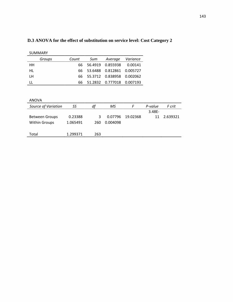
143

D.3 ANOVA for the effect of substitution on service level: Cost Category 2

SUMMARY Groups Count Sum Average Variance

HH 66 56.4919 0.855938 0.00141 HL 66 53.6488 0.812861 0.005727 LH 66 55.3712 0.838958 0.002062 LL 66 51.2832 0.777018 0.007193

ANOVA

Source of Variation SS df MS F P-value F crit

Between Groups 0.23388 3 0.07796 19.02368 3.48E-

11 2.639321 Within Groups 1.065491 260 0.004098

Total 1.299371 263

144

D.4 Tukey-Kramer Procedure for the effect of substitution on service level: Cost Category 2

Sample Sample

Group Mean Size 1. High,High 0.855937879 66

2. High,Low 0.812860606 66 3. Low,High 0.838957576 66 4. Low,Low 0.777018182 66

Other Data Level of significance 0.05 Numerator d.f. 4 Denominator d.f. 260 MSW 0.004098043 Q Statistic 3.73

Absolute Std. Error Critical

Comparison Difference of Difference Range Results Group 1 to Group 2 0.043077273 0.00787982 0.029391729 Difference

Group 1 to Group 3 0.016980303 0.00787982 0.029391729 No Difference

Group 1 to Group 4 0.078919697 0.00787982 0.029391729 Difference

Group 2 to Group 3 0.02609697 0.00787982 0.029391729 No Difference

Group 2 to Group 4 0.035842424 0.00787982 0.029391729 Difference

Group 3 to Group 4 0.061939394 0.00787982 0.029391729 Difference

145

D.5 ANOVA for the effect of substitution on service level: Cost Category 3

SUMMARY

Groups Count Sum Average Variance HH 42 37.9134 0.9027 0.000843 HL 42 37.2335 0.886512 0.002702 LH 42 38.2254 0.910129 0.000785 LL 42 36.9453 0.87965 0.003145

ANOVA

Source of Variation SS df MS F P-value F crit Between Groups 0.025014 3 0.008338 4.461842 0.004844 2.65972 Within Groups 0.306476 164 0.001869

Total 0.331491 167

146

D.6 Tukey-Kramer Procedure for the effect of substitution on service level: Cost Category 3

Sample Sample

Group Mean Size High, High 0.9027 42

High, Low 0.886512 42 Low, High 0.910129 42 Low, Low 0.87965 42

Other Data Level of

significance 0.05 Numerator d.f. 4 Denominator d.f. 164 MSW 0.001869 Q Statistic 3.79

Absolute Std. Error Critical

Comparison Difference

of Difference Range Results

Group 1 to Group 2 0.016188 0.00667 0.03 No Difference Group 1 to Group 3 0.007429 0.00667 0.03 No Difference Group 1 to Group 4 0.02305 0.00667 0.03 No Difference Group 2 to Group 3 0.023617 0.00667 0.03 No Difference Group 2 to Group 4 0.006862 0.00667 0.03 No Difference Group 3 to Group 4 0.030479 0.00667 0.03 Difference

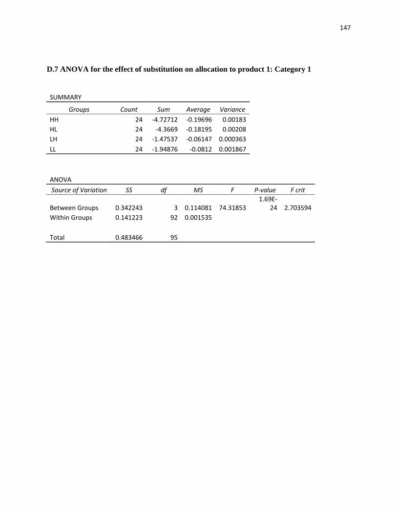
147

D.7 ANOVA for the effect of substitution on allocation to product 1: Category 1

SUMMARY Groups Count Sum Average Variance

HH 24 -4.72712 -0.19696 0.00183 HL 24 -4.3669 -0.18195 0.00208 LH 24 -1.47537 -0.06147 0.000363 LL 24 -1.94876 -0.0812 0.001867

ANOVA

Source of Variation SS df MS F P-value F crit

Between Groups 0.342243 3 0.114081 74.31853 1.69E-

24 2.703594 Within Groups 0.141223 92 0.001535

Total 0.483466 95

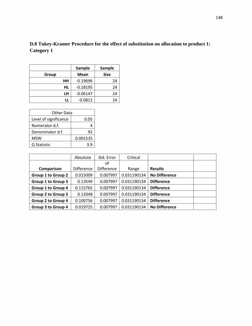
148

D.8 Tukey-Kramer Procedure for the effect of substitution on allocation to product 1: Category 1

Sample Sample Group Mean Size HH -0.19696 24

HL -0.18195 24 LH -0.06147 24 LL -0.0812 24

Other Data Level of significance 0.05 Numerator d.f. 4 Denominator d.f. 92 MSW 0.001535 Q Statistic 3.9

Absolute Std. Error Critical

Comparison Difference of

Difference Range Results Group 1 to Group 2 0.015009 0.007997 0.031190134 No Difference Group 1 to Group 3 0.13549 0.007997 0.031190134 Difference Group 1 to Group 4 0.115765 0.007997 0.031190134 Difference Group 2 to Group 3 0.12048 0.007997 0.031190134 Difference Group 2 to Group 4 0.100756 0.007997 0.031190134 Difference Group 3 to Group 4 0.019725 0.007997 0.031190134 No Difference

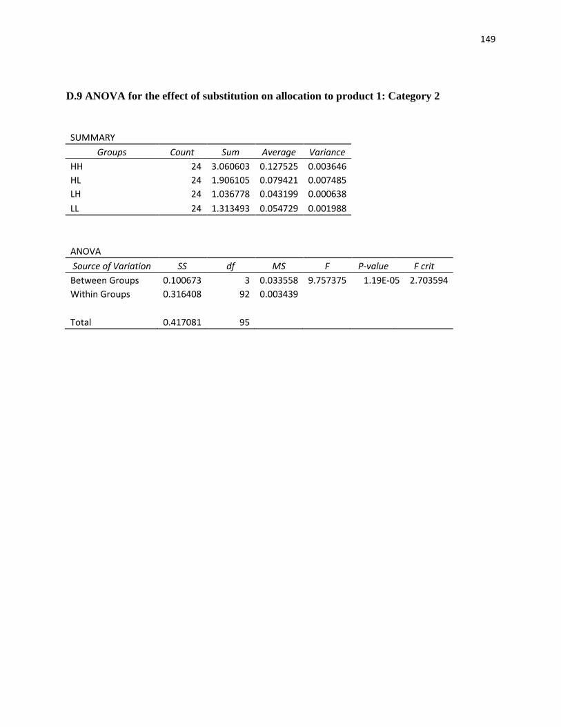
149

D.9 ANOVA for the effect of substitution on allocation to product 1: Category 2

SUMMARY

Groups Count Sum Average Variance HH 24 3.060603 0.127525 0.003646 HL 24 1.906105 0.079421 0.007485 LH 24 1.036778 0.043199 0.000638 LL 24 1.313493 0.054729 0.001988

ANOVA

Source of Variation SS df MS F P-value F crit Between Groups 0.100673 3 0.033558 9.757375 1.19E-05 2.703594 Within Groups 0.316408 92 0.003439

Total 0.417081 95

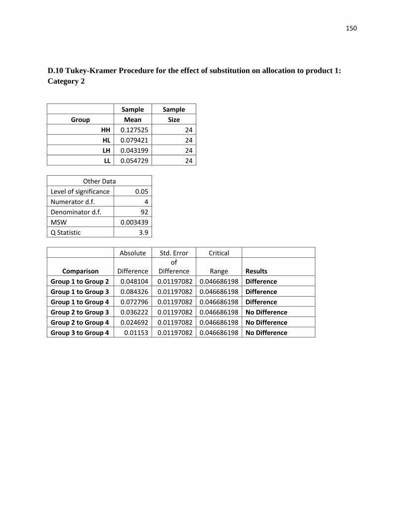
150

D.10 Tukey-Kramer Procedure for the effect of substitution on allocation to product 1: Category 2

Sample Sample Group Mean Size HH 0.127525 24

HL 0.079421 24 LH 0.043199 24 LL 0.054729 24

Other Data Level of significance 0.05 Numerator d.f. 4 Denominator d.f. 92 MSW 0.003439 Q Statistic 3.9

Absolute Std. Error Critical

Comparison Difference of

Difference Range Results Group 1 to Group 2 0.048104 0.01197082 0.046686198 Difference Group 1 to Group 3 0.084326 0.01197082 0.046686198 Difference Group 1 to Group 4 0.072796 0.01197082 0.046686198 Difference Group 2 to Group 3 0.036222 0.01197082 0.046686198 No Difference Group 2 to Group 4 0.024692 0.01197082 0.046686198 No Difference Group 3 to Group 4 0.01153 0.01197082 0.046686198 No Difference

151

D.11 Paired t-test for the effect of Cost properties on Service Level

Cost Level 1 Cost Level 2 Mean 0.67429881 0.894747619 Variance 0.009483518 0.001984975 Observations 168 168 Pearson Correlation 0.505851838

Hypothesized Mean Difference 0 df 167

t Stat -

33.96071439 P(T<=t) one-tail 3.44928E-77 t Critical one-tail 1.654029129 P(T<=t) two-tail 6.89857E-77 t Critical two-tail 1.974270919

D.12 Paired t-test for the effect of holding cost on service level

h = 0.5 h = 5 Mean 0.822064333 0.779252 Variance 0.011149402 0.013000037 Observations 300 300 Pearson Correlation 0.947330008 Hypothesized Mean Difference 0 df 299 t Stat 20.26295799 P(T<=t) one-tail 2.33304E-58 t Critical one-tail 1.649965768 P(T<=t) two-tail 4.66608E-58 t Critical two-tail 1.967929605

152

D.13 Paired t-test for the effect of shelf-life on mean service level.

m = 4 m=6 Mean 0.756335119 0.829082 Variance 0.019748449 0.006871 Observations 168 168 Pearson Correlation 0.857969079 Hypothesized Mean Difference 0 Df 167 t Stat -11.5792788 P(T<=t) one-tail 1.9424E-23 t Critical one-tail 1.654029129 P(T<=t) two-tail 3.8848E-23 t Critical two-tail 1.974270919

D.14 Paired t-test for the effect of lead time on mean service level.

No Lead Time Lead Time

Mean 0.757212 0.820762 Variance 0.017310626 0.011868 Observations 200 200 Pearson Correlation 0.845110038

Hypothesized Mean Difference 0 df 199 t Stat -12.77103216 P(T<=t) one-tail 5.67621E-28 t Critical one-tail 1.652546747 P(T<=t) two-tail 1.13524E-27 t Critical two-tail 1.971956498

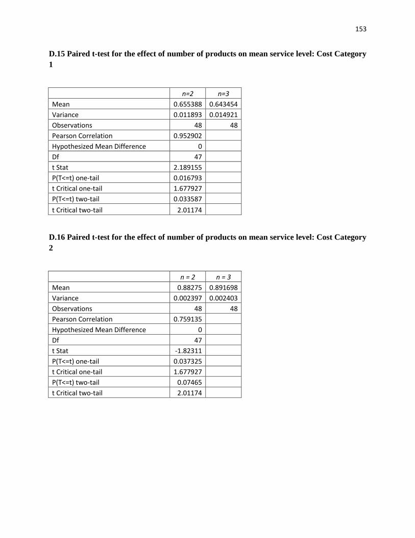
153

D.15 Paired t-test for the effect of number of products on mean service level: Cost Category 1

n=2 n=3 Mean 0.655388 0.643454 Variance 0.011893 0.014921 Observations 48 48 Pearson Correlation 0.952902

Hypothesized Mean Difference 0 Df 47 t Stat 2.189155 P(T<=t) one-tail 0.016793 t Critical one-tail 1.677927 P(T<=t) two-tail 0.033587 t Critical two-tail 2.01174

D.16 Paired t-test for the effect of number of products on mean service level: Cost Category 2

n = 2 n = 3 Mean 0.88275 0.891698 Variance 0.002397 0.002403 Observations 48 48 Pearson Correlation 0.759135 Hypothesized Mean Difference 0 Df 47 t Stat -1.82311 P(T<=t) one-tail 0.037325 t Critical one-tail 1.677927 P(T<=t) two-tail 0.07465 t Critical two-tail 2.01174

154

Appendix E: Tables from Heuristic Testing

E.1 Scenarios for Heuristic Testing

Key:

Sc.

Sc = Scenario, Dist = Distribution of daily product demand, μ = mean daily product demand, CV = coefficient of variation of product demand. R = length of review period in days, L = lead time in days, m1 = shelf-life of product 1 in days, m2 = shelf-life of product 2 in days, p1 = retail price of product 1, p2 = retail price of product 2, v1 = unit cost of product 1, v2 = unit cost of product 2, h = holding cost of applied to average inventory for length of simulation run, E(κ1) = expected market share of product 1, psub = level of product based substitution, asub = level of age-based substitution

Dist μ CV R L m1 m2 p1 p2 v1 v2 h E(κ1) psub asub 1 Gamma 10 0.7 1 0 4 4 8 8 3 3 3.46 0.50 High High 2 Gamma 5 0.7 2 0 4 4 5 5 1 1 4.11 0.50 Low High 3 Gamma 5 0.7 2 0 4 4 6 5 2 1 1.48 0.50 High Low 4 Gamma 8 0.7 2 1 4 4 7 5 3 1 2.48 0.55 High High 5 Gamma 8 0.7 3 0 4 4 5 7 1 3 2.86 0.55 High Low 6 Gamma 10 0.6 1 0 4 4 4 5 2 3 3.12 0.55 Low High 7 Gamma 8 0.6 2 0 4 4 3 3 1 1 3.00 0.60 High Low 8 Gamma 5 0.6 2 1 4 4 4 3 2 1 4.79 0.60 Low High 9 Gamma 5 0.6 2 1 4 4 3 5 1 3 3.61 0.60 Low Low

10 Gamma 7 0.6 2 0 4 4 4 3 2 1 4.96 0.65 High High 11 Gamma 12 0.5 1 0 4 4 6 6 1 1 2.96 0.65 Low High 12 Gamma 5 0.5 3 0 4 4 6 7 2 3 0.35 0.40 High High 13 Gamma 8 0.5 2 0 4 4 8 7 2 1 4.36 0.45 High High 14 Gamma 5 0.5 2 1 4 4 4 4 1 1 2.27 0.35 Low Low 15 Gamma 8 0.5 2 0 4 4 7 8 1 2 3.43 0.65 High High 16 Gamma 15 0.4 2 1 6 4 3 4 1 2 2.26 0.55 High Low 17 Gamma 15 0.4 1 0 6 4 5 4 2 1 0.46 0.40 High High 18 Gamma 15 0.4 1 1 6 4 7 7 2 2 3.59 0.50 High High 19 Gamma 15 0.4 2 1 6 4 5 6 1 2 3.59 0.30 High High 20 Gamma 15 0.4 1 0 6 4 8 8 3 3 0.72 0.35 Low High 21 Gamma 12 0.5 2 1 6 6 6 6 1 1 1.11 0.50 Low High 22 Gamma 12 0.5 3 0 6 6 4 4 2 2 2.40 0.60 Low High 23 Gamma 12 0.5 2 0 6 6 5 5 3 3 4.01 0.60 Low Low 24 Gamma 12 0.5 3 0 6 6 4 5 1 2 0.54 0.60 High Low 25 Gamma 12 0.5 1 0 6 6 5 4 2 1 4.36 0.65 High Low 26 Gamma 8 0.6 2 1 6 6 7 6 3 2 0.75 0.45 High Low

155

Sc. Dist μ CV R L m1 m2 p1 p2 v1 v2 h E(κ1) psub asub 27 Gamma 8 0.6 3 1 6 6 4 4 1 1 4.04 0.50 Low High 28 Gamma 8 0.6 3 0 6 6 5 5 1 1 4.44 0.55 High Low 29 Gamma 8 0.6 3 0 6 6 5 6 2 3 3.43 0.60 High Low 30 Gamma 8 0.6 4 0 6 6 5 6 1 2 0.66 0.35 Low Low 31 Gamma 6 0.6 3 0 8 6 6 8 1 3 3.78 0.55 High High 32 Gamma 6 0.6 4 0 8 6 4 4 1 1 0.73 0.60 High High 33 Gamma 6 0.6 3 0 8 6 6 5 2 1 0.12 0.60 Low Low 34 Gamma 6 0.6 4 1 8 6 6 7 2 3 1.05 0.35 Low High 35 Gamma 6 0.6 4 1 8 6 7 7 1 1 3.47 0.35 Low Low 36 Gamma 4 0.5 5 0 8 6 5 5 3 3 1.91 0.55 High Low 37 Gamma 4 0.5 3 1 8 6 4 4 2 2 0.96 0.60 High High 38 Gamma 4 0.5 2 1 8 6 5 5 1 1 4.41 0.60 High High 39 Gamma 4 0.5 4 0 8 6 7 6 2 1 1.19 0.60 Low Low 40 Gamma 4 0.5 5 0 8 6 4 5 1 2 3.89 0.65 High High 41 Gamma 5 0.5 4 0 8 8 6 6 1 1 4.23 0.55 High Low 42 Gamma 5 0.5 3 0 8 8 5 5 1 1 4.16 0.45 Low Low 43 Gamma 5 0.5 3 1 8 8 6 7 1 2 4.55 0.50 High Low 44 Gamma 5 0.5 3 1 8 8 3 4 1 2 2.68 0.60 High High 45 Gamma 5 0.5 5 0 8 8 5 4 2 1 3.54 0.35 High Low 46 Normal 10 0.3 5 0 8 8 7 6 2 1 1.50 0.45 High High 47 Normal 10 0.3 5 0 8 8 8 8 2 2 0.40 0.65 High High 48 Normal 10 0.3 3 1 8 6 7 7 1 1 2.10 0.60 Low Low 49 Normal 10 0.3 2 0 8 6 5 4 2 1 0.80 0.70 Low Low 50 Normal 10 0.3 2 0 8 6 6 6 1 1 3.20 0.40 High High 51 Normal 10 0.3 2 1 8 6 6 4 3 1 1.60 0.40 High High 52 Normal 10 0.3 2 1 8 6 8 8 2 2 0.50 0.50 High Low 53 Normal 10 0.3 3 0 8 6 6 7 3 4 0.60 0.60 High Low 54 Normal 8 0.3 2 1 6 6 5 5 1 1 1.80 0.40 Low High 55 Normal 8 0.3 4 0 6 6 4 3 2 1 2.40 0.60 Low High 56 Normal 8 0.3 3 1 6 6 8 8 3 3 1.90 0.50 High Low 57 Normal 8 0.3 3 1 6 6 7 6 2 1 2.40 0.60 High Low 58 Normal 8 0.3 3 0 6 6 6 7 1 2 3.70 0.45 Low High 59 Normal 8 0.3 2 0 6 6 4 4 2 2 2.90 0.40 Low High 60 Normal 10 0.3 2 1 6 4 5 5 1 1 4.10 0.55 High Low 61 Normal 10 0.3 2 1 6 4 5 4 2 1 1.20 0.50 High Low 62 Normal 10 0.3 1 0 6 4 4 5 1 2 0.40 0.50 Low Low 63 Normal 15 0.3 2 0 4 4 6 6 1 1 2.70 0.35 High High 64 Normal 15 0.3 2 0 4 4 4 4 2 2 3.20 0.40 Low High 65 Normal 15 0.3 1 0 4 4 5 4 2 1 1.30 0.45 Low Low 66 Normal 15 0.3 2 1 4 4 8 7 2 1 0.40 0.60 High High

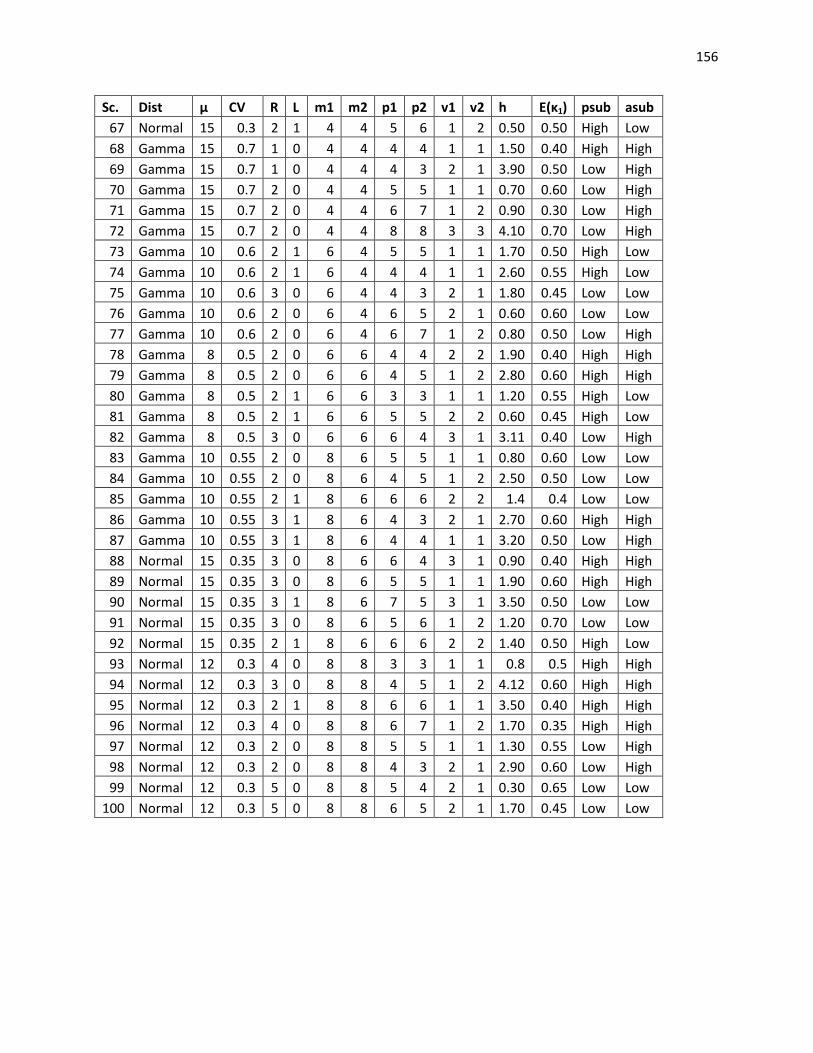
156

Sc. Dist μ CV R L m1 m2 p1 p2 v1 v2 h E(κ1) psub asub 67 Normal 15 0.3 2 1 4 4 5 6 1 2 0.50 0.50 High Low 68 Gamma 15 0.7 1 0 4 4 4 4 1 1 1.50 0.40 High High 69 Gamma 15 0.7 1 0 4 4 4 3 2 1 3.90 0.50 Low High 70 Gamma 15 0.7 2 0 4 4 5 5 1 1 0.70 0.60 Low High 71 Gamma 15 0.7 2 0 4 4 6 7 1 2 0.90 0.30 Low High 72 Gamma 15 0.7 2 0 4 4 8 8 3 3 4.10 0.70 Low High 73 Gamma 10 0.6 2 1 6 4 5 5 1 1 1.70 0.50 High Low 74 Gamma 10 0.6 2 1 6 4 4 4 1 1 2.60 0.55 High Low 75 Gamma 10 0.6 3 0 6 4 4 3 2 1 1.80 0.45 Low Low 76 Gamma 10 0.6 2 0 6 4 6 5 2 1 0.60 0.60 Low Low 77 Gamma 10 0.6 2 0 6 4 6 7 1 2 0.80 0.50 Low High 78 Gamma 8 0.5 2 0 6 6 4 4 2 2 1.90 0.40 High High 79 Gamma 8 0.5 2 0 6 6 4 5 1 2 2.80 0.60 High High 80 Gamma 8 0.5 2 1 6 6 3 3 1 1 1.20 0.55 High Low 81 Gamma 8 0.5 2 1 6 6 5 5 2 2 0.60 0.45 High Low 82 Gamma 8 0.5 3 0 6 6 6 4 3 1 3.11 0.40 Low High 83 Gamma 10 0.55 2 0 8 6 5 5 1 1 0.80 0.60 Low Low 84 Gamma 10 0.55 2 0 8 6 4 5 1 2 2.50 0.50 Low Low 85 Gamma 10 0.55 2 1 8 6 6 6 2 2 1.4 0.4 Low Low 86 Gamma 10 0.55 3 1 8 6 4 3 2 1 2.70 0.60 High High 87 Gamma 10 0.55 3 1 8 6 4 4 1 1 3.20 0.50 Low High 88 Normal 15 0.35 3 0 8 6 6 4 3 1 0.90 0.40 High High 89 Normal 15 0.35 3 0 8 6 5 5 1 1 1.90 0.60 High High 90 Normal 15 0.35 3 1 8 6 7 5 3 1 3.50 0.50 Low Low 91 Normal 15 0.35 3 0 8 6 5 6 1 2 1.20 0.70 Low Low 92 Normal 15 0.35 2 1 8 6 6 6 2 2 1.40 0.50 High Low 93 Normal 12 0.3 4 0 8 8 3 3 1 1 0.8 0.5 High High 94 Normal 12 0.3 3 0 8 8 4 5 1 2 4.12 0.60 High High 95 Normal 12 0.3 2 1 8 8 6 6 1 1 3.50 0.40 High High 96 Normal 12 0.3 4 0 8 8 6 7 1 2 1.70 0.35 High High 97 Normal 12 0.3 2 0 8 8 5 5 1 1 1.30 0.55 Low High 98 Normal 12 0.3 2 0 8 8 4 3 2 1 2.90 0.60 Low High 99 Normal 12 0.3 5 0 8 8 5 4 2 1 0.30 0.65 Low Low

100 Normal 12 0.3 5 0 8 8 6 5 2 1 1.70 0.45 Low Low

157

E.2 Comparison of Heuristic Solution to Simulated Optimal Solution

Key:

Sc = scenario, S1 = Order-up-to level of Product 1, S2 = Order up to level of Product 2, Profit = Mean profit obtained for scenario after k replications, stdev = standard deviation of the profit after K replications for each scenario, K = number of replications, ENVR = extended newsvendor heuristic, NVR = newsvendor heuristic.

ENVR NVR Simulated-Optimal

Sc. S1 S2 Profit stdev K S1 S2 Profit stdev K S1* S2* Profit* stdev K

1 8 8 2464.15 214.28 74 6 5 2219.2 152.66 46 10 7 2469.23 252.2 102

2 7 7 982.38 96.94 94 7 7 982.38 96.94 94 8 6 996.76 82.11 66

3 5 7 903.16 91.45 139 7 6 877.61 93.18 196 5 9 911.76 103.7 221

4 13 19 1447.91 166.69 227 15 12 1405.25 154.29 206 8 25 1458.7 155.9 195

5 16 8 1028.25 146.18 290 15 13 949.1 167.67 290 20 5 1050.47 142 290

6 9 6 935.93 96.02 103 5 4 812.44 47.32 33 9 6 935.93 96.02 103

7 11 8 700.36 67.67 160 11 8 700.36 67.67 160 11 8 700.36 67.67 160

8 9 8 413.99 50.64 256 10 6 408.92 49.6 252 8 7 417.52 42.1 175

9 10 5 368.2 45.85 266 9 6 362.48 48.07 290 10 4 370.55 42.61 227

10 8 8 635.08 59.2 149 9 5 622.56 47.63 100 7 8 636.17 47.33 96

11 15 8 3303.64 225.72 80 12 6 3225.05 196.29 24 16 8 3304.54 231.9 85

12 7 8 872.11 65.92 98 6 10 857.4 79 113 8 7 877.19 65.3 96

13 8 15 2559.89 172.24 78 9 12 2549.62 167.35 74 7 16 2563.64 172.7 78

14 7 12 669.9 61.7 145 6 12 669.64 59.06 133 7 13 670.35 62.7 150

15 16 7 2600.97 174.74 79 13 7 2555.71 158.11 66 16 7 2600.97 174.7 79

16 36 13 1443.63 91.26 69 26 21 1418.21 85.77 63 32 16 1450.26 84.44 59

17 11 15 2516.23 134.69 111 7 11 2424.22 105.67 73 10 14 2524.36 132.6 106

18 22 15 4048.92 228.43 31 17 17 3967.62 197.03 27 23 17 4091.54 238.3 33

19 30 24 3148.22 157.92 98 14 32 3045.81 141.86 83 30 27 3165.33 168.4 110

20 10 14 4126.66 220.17 110 6 11 3882.44 164.65 70 10 14 4126.66 220.2 110

21 25 24 3237.41 238.4 53 23 23 3219.53 231.79 55 29 27 3257.6 249.1 57

22 22 15 1160.35 83.36 51 21 14 1149.74 72.07 38 23 14 1161.29 83.47 51

23 16 10 1016.77 100.58 94 13 8 1015.63 73.26 50 14 10 1033.44 91.71 77

24 27 13 1808.62 121.74 45 24 16 1801.36 127.41 49 30 13 1821.66 133.1 52

25 14 12 1834.37 156.88 67 9 5 1846.57 150.8 65 10 10 1884.57 158.2 66

26 11 16 1449.88 137.84 87 12 14 1446.11 136.5 87 10 19 1460.69 144.3 95

27 20 20 1162.77 114.01 93 19 19 1160.01 110.89 88 21 20 1163.66 114.3 93

28 17 13 1552.55 128.66 67 17 14 1553.17 131.1 69 16 16 1557.59 136.5 75

29 15 8 1067.09 86.2 63 15 10 1075.6 95.34 77 17 10 1081.02 103.2 88

30 14 21 1246.39 146.1 132 13 24 1230.66 150.61 145 14 17 1265.34 128.4 100

31 16 6 1522.6 120.66 62 12 10 1529.86 125.46 66 17 8 1551.29 131.5 70

32 19 10 937.62 84.3 80 17 12 904.53 92.97 93 23 8 951.35 92.66 91

158

ENVR NVR Simulated-Optimal

Sc. S1 S2 Profit stdev K S1 S2 Profit stdev K S1* S2* Profit* stdev K

33 14 9 1185.3 108.52 81 13 8 1143.21 98.79 26 13 10 1189.61 110.1 83

34 14 19 1101.22 118.9 109 11 21 1064.61 113.93 106 15 17 1113.68 115 101

35 14 23 1585.54 162.06 104 14 25 1525.46 164.04 106 18 20 1602.78 158.1 94

36 10 6 289.6 29.54 179 10 9 255.54 39.1 339 10 6 289.6 27.56 158

37 11 6 392.73 34.81 141 10 6 386.53 31.81 151 11 6 392.73 34.81 141

38 10 6 849.56 61.14 89 9 6 843.56 58.62 83 10 6 849.56 61.14 89

39 11 8 938.11 75.87 112 11 8 938.11 75.87 112 11 8 938.11 75.87 112

40 16 5 555.22 43.9 107 14 8 547.45 46.25 123 16 5 555.22 43.9 107

41 14 11 1289.55 112.39 73 14 11 1289.55 112.39 73 13 13 1292 116.4 78

42 9 11 962.66 75.79 60 9 10 959.2 70.08 52 10 13 968.65 85.8 76

43 15 10 1206.9 97.67 63 12 12 1195.99 90.19 55 17 10 1219.76 80 111

44 15 8 488.5 46.68 88 13 8 478.74 37.96 61 15 8 488.5 46.68 88

45 7 19 604.75 59.94 290 10 18 587.6 64.21 290 7 16 608.49 49.84 259

46 20 35 2604.19 148.26 125 25 31 2598.07 148.47 127 21 31 2620.28 131.5 97

47 35 19 3145.49 173.93 118 36 19 3140.04 183.35 132 31 21 3150.06 168.6 112

48 29 18 3159.49 167.72 109 28 19 3167.61 161.48 101 29 21 3175.49 170.7 112

49 17 8 1611.39 77.65 71 15 7 1593.03 67.96 71 17 8 1611.39 77.65 71

50 12 14 2854.44 125.78 76 10 15 2842.95 121.51 72 12 14 2855.28 126.7 76

51 12 22 1661.83 78.87 87 13 19 1650.69 73.51 77 13 22 1666.95 80.6 91

52 20 15 3299.78 155.47 87 17 17 3274.62 153.79 85 22 15 3321.91 166.8 97

53 21 9 1528.34 87.38 127 18 12 1545.11 79.1 101 18 12 1545.11 79.1 101

54 12 17 1773.39 87.63 95 11 17 1764.98 82.6 85 13 19 1779.6 87.4 93

55 18 15 747.51 48.24 160 20 13 743.06 50.14 176 18 13 749.17 47.1 153

56 17 16 2035.58 132.59 164 17 17 2036.65 132.96 164 16 17 2039.03 127.9 152

57 18 18 2096.19 126.69 141 22 14 2088.11 127.05 145 19 19 2105.04 127.5 142

58 14 14 2191.23 91.88 67 12 15 2190.42 93.37 70 14 16 2207.95 108 91

59 8 11 836.01 46.1 118 6 10 818.93 33.58 66 7 11 843.29 39.2 85

60 22 13 2056.49 104.6 100 19 16 2059.5 94.2 84 22 18 2072.07 101.6 93

61 17 17 1531.08 74.99 94 17 16 1527.69 73.23 89 15 20 1538.7 74.37 90

62 9 6 1682.38 77 81 6 6 1652.25 70.87 71 9 6 1682.38 77 81

63 13 24 4230.07 179.7 71 13 24 4224.19 186.02 76 14 22 4231.19 178.1 69

64 12 19 1530.21 67.18 76 12 18 1515.39 67.18 76 13 19 1534.39 73.44 89

65 9 13 2404.04 117.92 93 8 10 2381.88 106.59 78 9 12 2404.84 117.3 93

66 26 27 4950.21 222.71 79 31 21 4920.71 226.8 83 27 29 4961.34 224.5 79

67 30 21 3085.75 161.83 107 25 25 3078.42 165.16 111 31 21 3111.95 181.8 132

68 13 20 2335.53 229.78 93 8 12 2181.57 170.62 59 13 20 2335.53 229.8 93

69 14 16 1367.03 170.22 597 8 7 1250.25 86.38 184 9 16 1417 145.9 409

70 26 17 3096.88 279.26 79 25 17 3087.79 276.39 77 26 18 3112.06 286.5 82

71 15 26 3802 349.28 82 12 27 3754.82 339.36 75 27 14 3802.49 350.5 82

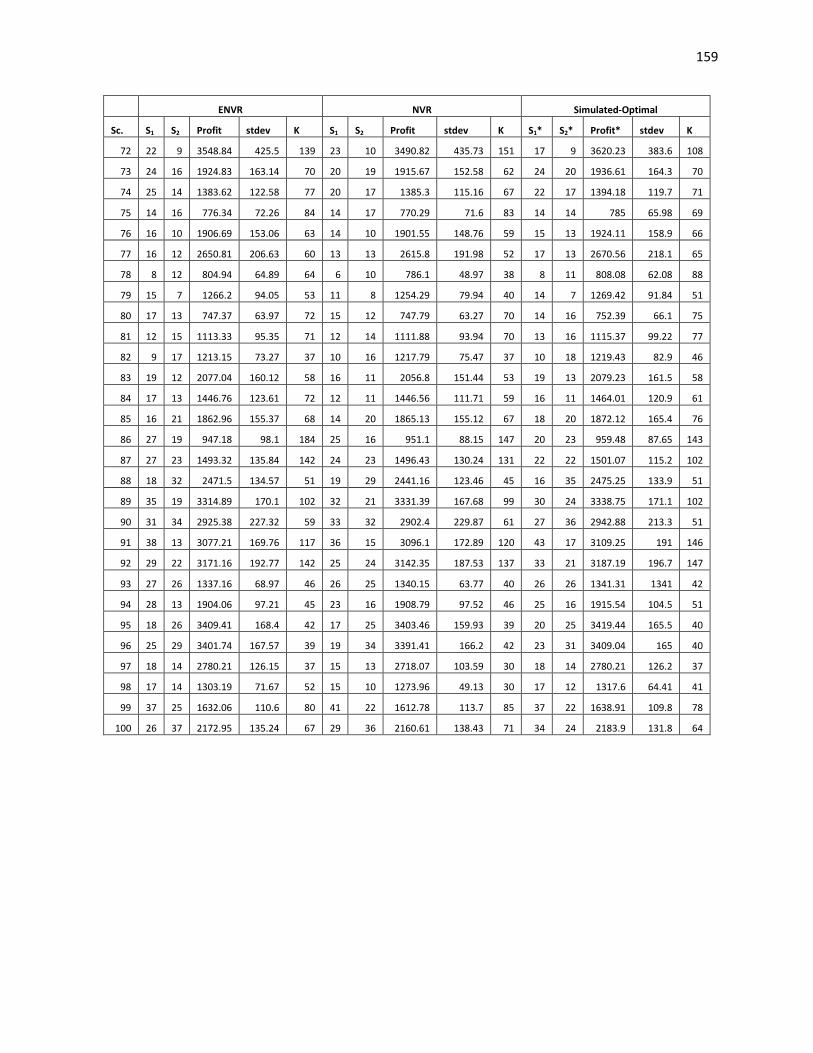
159

ENVR NVR Simulated-Optimal

Sc. S1 S2 Profit stdev K S1 S2 Profit stdev K S1* S2* Profit* stdev K

72 22 9 3548.84 425.5 139 23 10 3490.82 435.73 151 17 9 3620.23 383.6 108

73 24 16 1924.83 163.14 70 20 19 1915.67 152.58 62 24 20 1936.61 164.3 70

74 25 14 1383.62 122.58 77 20 17 1385.3 115.16 67 22 17 1394.18 119.7 71

75 14 16 776.34 72.26 84 14 17 770.29 71.6 83 14 14 785 65.98 69

76 16 10 1906.69 153.06 63 14 10 1901.55 148.76 59 15 13 1924.11 158.9 66

77 16 12 2650.81 206.63 60 13 13 2615.8 191.98 52 17 13 2670.56 218.1 65

78 8 12 804.94 64.89 64 6 10 786.1 48.97 38 8 11 808.08 62.08 88

79 15 7 1266.2 94.05 53 11 8 1254.29 79.94 40 14 7 1269.42 91.84 51

80 17 13 747.37 63.97 72 15 12 747.79 63.27 70 14 16 752.39 66.1 75

81 12 15 1113.33 95.35 71 12 14 1111.88 93.94 70 13 16 1115.37 99.22 77

82 9 17 1213.15 73.27 37 10 16 1217.79 75.47 37 10 18 1219.43 82.9 46

83 19 12 2077.04 160.12 58 16 11 2056.8 151.44 53 19 13 2079.23 161.5 58

84 17 13 1446.76 123.61 72 12 11 1446.56 111.71 59 16 11 1464.01 120.9 61

85 16 21 1862.96 155.37 68 14 20 1865.13 155.12 67 18 20 1872.12 165.4 76

86 27 19 947.18 98.1 184 25 16 951.1 88.15 147 20 23 959.48 87.65 143

87 27 23 1493.32 135.84 142 24 23 1496.43 130.24 131 22 22 1501.07 115.2 102

88 18 32 2471.5 134.57 51 19 29 2441.16 123.46 45 16 35 2475.25 133.9 51

89 35 19 3314.89 170.1 102 32 21 3331.39 167.68 99 30 24 3338.75 171.1 102

90 31 34 2925.38 227.32 59 33 32 2902.4 229.87 61 27 36 2942.88 213.3 51

91 38 13 3077.21 169.76 117 36 15 3096.1 172.89 120 43 17 3109.25 191 146

92 29 22 3171.16 192.77 142 25 24 3142.35 187.53 137 33 21 3187.19 196.7 147

93 27 26 1337.16 68.97 46 26 25 1340.15 63.77 40 26 26 1341.31 1341 42

94 28 13 1904.06 97.21 45 23 16 1908.79 97.52 46 25 16 1915.54 104.5 51

95 18 26 3409.41 168.4 42 17 25 3403.46 159.93 39 20 25 3419.44 165.5 40

96 25 29 3401.74 167.57 39 19 34 3391.41 166.2 42 23 31 3409.04 165 40

97 18 14 2780.21 126.15 37 15 13 2718.07 103.59 30 18 14 2780.21 126.2 37

98 17 14 1303.19 71.67 52 15 10 1273.96 49.13 30 17 12 1317.6 64.41 41

99 37 25 1632.06 110.6 80 41 22 1612.78 113.7 85 37 22 1638.91 109.8 78

100 26 37 2172.95 135.24 67 29 36 2160.61 138.43 71 34 24 2183.9 131.8 64

160

E.3 t-test for Differences in Means between Heuristics and Simulation-Optimal Profit

Key: Sc. = Scenario, tstat = t-test statistic, tcrit = t critical value assuming a level of significance of 0.05 for two sample t-test assuming unequal population variances

ENVR NVR

Sc. tstat tcrit Result tstat tcrit Result 1 0.14 1.65 no difference 7.44 1.66 Difference 2 1.01 1.65 no difference 1.01 1.65 no difference 3 0.82 1.65 no difference 3.54 1.65 Difference 4 0.69 1.65 no difference 3.45 1.65 Difference 5 1.86 1.65 difference 7.86 1.65 Difference 6 0.00 1.65 no difference 9.84 1.66 Difference 7 0.00 1.65 no difference 0.00 1.65 no difference 8 0.79 1.65 no difference 1.93 1.65 Difference 9 0.59 1.65 no difference 2.02 1.65 Difference

10 0.16 1.65 no difference 2.01 1.65 Difference 11 0.03 1.65 no difference 1.68 1.68 no difference 12 0.54 1.65 no difference 1.98 1.65 Difference 13 0.14 1.65 no difference 0.51 1.66 no difference 14 0.06 1.65 no difference 0.10 1.65 no difference 15 0.00 1.65 no difference 1.64 1.66 no difference 16 0.43 1.66 no difference 2.08 1.66 Difference 17 0.45 1.65 no difference 5.61 1.65 Difference 18 0.73 1.67 no difference 2.21 1.67 Difference 19 0.76 1.65 no difference 5.34 1.65 Difference 20 0.00 1.65 no difference 8.49 1.65 Difference 21 0.43 1.66 no difference 0.84 1.66 no difference 22 0.06 1.66 no difference 0.70 1.66 no difference 23 1.13 1.65 no difference 1.21 1.66 no difference 24 0.50 1.66 no difference 0.78 1.66 no difference 25 1.84 1.66 difference 1.41 1.66 no difference 26 0.52 1.65 no difference 0.70 1.65 no difference 27 0.05 1.65 no difference 0.22 1.65 no difference 28 0.23 1.66 no difference 0.20 1.66 no difference 29 0.90 1.66 no difference 0.35 1.65 no difference 30 1.05 1.65 no difference 1.93 1.65 Difference 31 1.31 1.66 no difference 0.97 1.66 no difference 32 1.01 1.65 no difference 3.42 1.65 Difference

161

ENVR NVR Sc. tstat tcrit Result tstat tcrit Result

33 0.25 1.65 no difference 2.03 1.68 Difference 34 0.77 1.65 no difference 3.08 1.65 Difference 35 0.76 1.65 no difference 3.39 1.65 Difference 36 0.00 1.65 no difference 11.16 1.65 Difference 37 0.00 1.65 no difference 1.59 1.65 no difference 38 0.00 1.65 no difference 0.66 1.65 no difference 39 0.00 1.65 no difference 0.00 1.65 no difference 40 0.00 1.65 no difference 1.31 1.65 no difference 41 0.13 1.66 no difference 0.13 1.66 no difference 42 0.43 1.66 no difference 0.68 1.66 no difference 43 0.89 1.66 no difference 1.66 1.66 no difference 44 0.00 1.65 no difference 1.40 1.66 no difference 45 0.80 1.65 no difference 4.28 1.65 Difference 46 0.86 1.65 no difference 1.18 1.65 no difference 47 0.20 1.65 no difference 0.44 1.65 no difference 48 0.70 1.65 no difference 0.35 1.65 no difference 49 0.00 1.66 no difference 1.50 1.66 no difference 50 0.04 1.66 no difference 0.60 1.66 no difference 51 0.43 1.65 no difference 1.37 1.65 no difference 52 0.93 1.65 no difference 1.99 1.65 Difference 53 1.52 1.65 no difference 0.00 1.65 no difference 54 0.49 1.65 no difference 1.15 1.65 no difference 55 0.31 1.65 no difference 1.14 1.65 no difference 56 0.24 1.65 no difference 0.16 1.65 no difference 57 0.59 1.65 no difference 1.13 1.65 no difference 58 1.05 1.65 no difference 1.10 1.65 no difference 59 1.21 1.65 no difference 4.11 1.66 Difference 60 1.05 1.65 no difference 0.85 1.65 no difference 61 0.69 1.65 no difference 1.00 1.65 no difference 62 0.00 1.65 no difference 2.51 1.66 Difference 63 0.04 1.66 no difference 0.23 1.66 no difference 64 0.38 1.65 no difference 1.73 1.65 Difference 65 0.05 1.65 no difference 1.34 1.65 no difference 66 0.31 1.65 no difference 1.15 1.65 no difference 67 1.18 1.65 no difference 1.51 1.65 no difference 68 0.00 1.65 no difference 4.73 1.66 Difference 69 4.98 1.65 difference 17.33 1.65 Difference 70 0.34 1.65 no difference 0.54 1.65 no difference 71 0.01 1.65 no difference 0.87 1.65 no difference

162

ENVR NVR

Sc. tstat tcrit Result tstat tcrit Result 72 1.38 1.65 no difference 2.53 1.65 Difference 73 0.43 1.66 no difference 0.76 1.66 no difference 74 0.53 1.66 no difference 0.44 1.66 no difference 75 0.77 1.66 no difference 1.32 1.66 no difference 76 0.63 1.66 no difference 0.82 1.66 no difference 77 0.52 1.66 no difference 1.44 1.66 no difference 78 0.30 1.66 no difference 2.13 1.66 Difference 79 0.18 1.66 no difference 0.84 1.66 no difference 80 0.47 1.66 no difference 0.43 1.66 no difference 81 0.13 1.66 no difference 0.22 1.66 no difference 82 0.37 1.66 no difference 0.09 1.66 no difference 83 0.07 1.66 no difference 0.76 1.66 no difference 84 0.81 1.66 no difference 0.82 1.66 no difference 85 0.34 1.66 no difference 0.26 1.66 no difference 86 1.19 1.65 no difference 0.81 1.65 no difference 87 0.48 1.65 no difference 0.29 1.65 no difference 88 0.14 1.66 no difference 1.30 1.66 no difference 89 1.00 1.65 no difference 0.31 1.65 no difference 90 0.42 1.66 no difference 0.97 1.66 no difference 91 1.44 1.65 no difference 0.59 1.65 no difference 92 0.70 1.65 no difference 1.97 1.65 Difference 93 0.02 1.68 no difference 0.01 1.68 no difference 94 0.56 1.66 no difference 0.33 1.66 no difference 95 0.27 1.66 no difference 0.44 1.66 no difference 96 0.20 1.66 no difference 0.48 1.66 no difference 97 0.00 1.67 no difference 2.21 1.67 Difference 98 1.02 1.66 no difference 3.24 1.67 Difference 99 0.39 1.65 no difference 1.49 1.65 no difference

100 0.47 1.66 no difference 1.00 1.66 no difference

163

Vita

Bret Rothschild Myers was born in Richmond, Virginia. He attended the University of Richmond where he earned a BS in Business Administration with a concentration in Management Systems and minor in Spanish. While also at University of Richmond he was a 4 year member of the men’s varsity soccer team. His career as a soccer player led to two years of professional soccer with the USL A-League Richmond Kickers and also a gold medal with the US soccer team in the 11th Pan American Maccabi games. After his professional soccer stint, he earned an MS in Systems Engineering from the University of Virginia and has recently earned his Ph.D. in Decision Sciences within in the Lebow College of Business at Drexel University.

Dr. Myers has seven years of teaching experience in higher education. While at the University of Richmond, he served as a teaching assistant in Spanish. His work as a teaching assistant continued through his graduate studies at both the University of Virginia and at Drexel University. While working on his Ph.D. at Drexel University, he accepted a position as part-time faculty at Villanova University and was later promoted to full-time. At Villanova, Dr. Myers taught courses at the undergraduate and MBA level in both Statistics and Operations Management. Most recently, he has accepted a full-time position as Associate Professor in Management at Kutztown University.

Dr. Myers has co-authored articles in the proceedings of the Southwest Academy of Management and Indian Journal of Economics. He has made presentations at both the Southwest Academy of Management and Drexel University Research Day. At the University of Richmond, he also made contributions to the Spanish textbook, Dicho y Hecho, by Laila M. Dawson.